Embed Size (px)
Citation preview
CEGE 3502 FLUID MECHANICS
Lab Manual
(Spring 2016 Edition)
Originally prepared by: Maria Bergstedt (Fall 2001)
Revised over the years by number of academic staff, including:
Michele Guala; John S. Gulliver; Kimberly Hill; Ben Janke;
Corey Markfort; Qin Qian; Fotis Sotiropoulos; Craig Taylor; Jim Thill,
Jon Czuba
Most recently revised by K. Hill (Fall, 2015), J. Czuba and M. Guala (Spring, 2016)
Course textbook:
Engineering Fluid Mechanics, 9th or 10
th Ed.
Crowe, Elger, Williams, Roberson
John Wiley and Sons, New York, NY, 2009.
(all references to page numbers refer to the 9th edition of this textbook. Updates, hints, etc. will
be posted online Fall, 2014. Please check: http://www.ce.umn.edu/classpages/ce3502/)

2

3
4
TABLE OF CONTENTS
Section Page
General Instructions 5
Lab #1 Evaluation of Fluid Properties 8
Lab #2 Pressure & Velocity Measurement 15
Lab #3 Applications of the Bernoulli Equation 19
Lab #4 Applications of the Momentum Theorem 25
Lab #5 Turbulence and Boundary Layer Demonstration 30
Lab #6 Measurements of Pipe Friction 32
Lab #7 Pipe Bends 36
Lab #8 Pipe Networks 38
Lab #9 Pump Performance & Pump Sizing 43
Appendix A: Useful Equations 47
Appendix B: Integration Techniques 49
Appendix C: Minor Loss Coefficients 50
Appendix D: User’s Manual for Pump Testing Stand 51
Appendix E: Moody Diagram 57

5
6
CE 3502 FLUID MECHANICS LABORATORY
GENERAL INSTRUCTIONS
INTRODUCTION
The Fluid Mechanics Laboratory is a substantial part of CE 3502 and is constructed to
complement the lecture portion of the course. The labs are designed to provide the student with a
physical understanding of the fundamental principles and basic equations of fluid mechanics.
This understanding is gained through the application of “text book” concepts and equations to
real problems.
COURSE REQUIREMENTS
Attendance is required for all of the lab sessions. Each session, except one demonstration
activity, requires the completion of a formal lab report. These reports are the basis of your final
lab grade. With only eight assignments, each represents a substantial fraction of your total score.
LABORATORY PROCEDURE
1. The student is to read the lab manual chapter assigned to each laboratory period BEFORE
coming to the lab. Some labs contain thought questions or require that you perform some
derivations before proceeding. In addition, the appendix contains useful information for
many of the labs.
2. The class will work in groups to collect data for each set of experiments. It is desirable that
groups are limited to three students, but some students will learn more efficiently in a smaller
group, and some labs will require more students to work together to collect the data; it is still
recommended that groups of no more than three work together to analyze the data. Some
laboratory reports will be written by individuals and some submitted as group reports. This
is detailed in #4 below.
3. In carrying out the experiments the following points are important:
a) Before starting any experiment, clearly define the goals. What question are you
answering or what principle are you trying to demonstrate? What data is needed to
solve the problem? The graduate instructor for each lab will help outline some
necessary points, but it is ultimately it is each student’s responsibility to digest this
information for the laboratory report, and, ultimately for class exams.
b) Identify the methods of measurement and instrumentation to be used. At the research
stations, “play around” with the equipment so that you understand how the
instruments work, what you are measuring, and how what you are measuring
connects with the physics of the problems at hand.
7
c) Perform the experiment. Collect data in a clear and organized fashion. Be sure to
note the units for each measurement. Also, be sure to participate in the experiment
rather than just recording data for your group.
d) Perform your calculations before leaving the lab if time allows. This can help you to
better understand the concepts and equations presented in lab, and allow you to spot
data collection errors while there is still time to take new measurements.
e) Write your group’s formal report. This will be an easier task if done soon after lab
while the concepts are fresh in your mind. Students who wait for the last minute
often discover unanticipated problems.
4. Formal reports will be due one week after the experiment was performed. There will be
some reports you will submit with your group (recommended: 3 people) and some reports
you submit as an individual. These will be announced the day of the lab (if not sooner). In
either case, feel free to work with classmates, but the final report should reflect the
understanding and work performed by authors on the report. In no case should anything other
than the raw data be copied from other students’ work.
5. Every report except one is graded on the basis of 100 possible points. The demonstration lab
is much shorter, and carries the weight of 50 points. Absences can be made up only with
permission of the instructor and, subsequently, by coordinating with the teaching assistant of
your particular laboratory. Unfortunately, this cannot be done during another laboratory
meeting period because the enrollment in each laboratory is so high.
6. The policy for late laboratory reports is as follows: The first day the laboratory is late will
carry a 5% penalty. Each subsequent week late (starting with the second day the laboratory
is late will carry an additional 10% penalty.
FORMAL REPORT
Formal reports should be completed with a computer, including all final calculations, charts, and
data tables. The report should consist of the following sections:
1. Title page: Should contain:
(a) title of experiment
(b) laboratory section
(c) each author’s name (one for individual reports, each group member up to 4 for group
reports)
(d) Name of your TA
(e) Date on which the experiment was performed
(f) Signed and dated statement of honor (e.g. we did this work ourselves, etc.)
The names of other group members who aren’t authors (i.e., those whose raw data is likely
identical to the contents of this laboratory report) should be given at the bottom right-hand
corner of the title page.
8
2. Purpose of the experiment: State the overall objective of the laboratory exercise first and
then explain the objective of each particular experiment.
3. Apparatus and procedure: Briefly explain the procedure followed in the experiment. A
concise explanation of the equations to be used in the computations should be given.
Derivations of these equations are not necessary unless specifically indicated by the
instructor or the manual. Much information regarding the instruments and procedures is
included in the manual. You need not repeat it in the report. However, reference all
information in your summary to specific page numbers in the manual or other reference
material.
4. Tabulation of computed results: Computed results should be presented in a neat table with
all rows and columns clearly defined. Specify the correct units at the heading of each column
(row) in the table. Specify all units clearly.
5. Sample calculation: Show one complete set of typical calculations explaining step-by step
how the results have been computed (for each type of calculation). One set of actual readings
taken in the experiment should be used in the sample calculations. Units should be specified
for all computed quantities. Handwritten calculations are OK here, but keep them neat and
organized. Specify all units clearly.
6. Discussion: Discuss the results obtained and summarize your conclusions. This section
should answer any questions that are stated or implied in the purpose. Assumptions made,
difficulties encountered during the experiment, percentage error, and possible sources of
error should also be included in the discussion. Some labs may require extensive discussion
(a few paragraphs), while others may require just a few sentences. Note: Questions to be
answered may be in the text of this laboratory manual. Look carefully to be sure you
answer all the questions asked. Specify all units clearly.
7. Appendix: The raw data taken during the experiment, any handout sheets, and your response
to the thought questions will form the appendix of the report. Specify all units clearly.
Your calculations and conclusions are the cornerstones of your report. Show units on all
calculations (including intermediate steps) and in the results table(s), and always use an
appropriate number of significant digits. Proper organization of the report and adequate
presentation of the results will be given substantial weight in grading the work, as well.
The textbook referenced in this manual is:
Crowe, Elger, and Roberson, Engineering Fluid Mechanics, 9th ed, 2012 (John Wiley &
Sons, New York).
9
CE 3502 FLUID MECHANICS
Laboratory Experiment #1
EVALUATION OF FLUID PROPERTIES
The solution of engineering problems in fluid mechanics requires numerical values for certain
basic physical characteristics of the fluid of interest. These values are obtained by measurements
using commercially available instruments and standard procedures. In this laboratory session,
some fundamental properties of liquids will be measured. This lab is intended to familiarize the
student with a basic understanding of several important properties used to describe fluids.
These are the fluid properties, and appropriate measurement devices, which we will use:
1. Density, specific gravity or specific weight using a hydrometer and a hydrometric or
Westphal balance.
2. Absolute and kinematic viscosity using a Brookfield (rotational) viscometer and an
Ostwald or capillary viscometer.
3. Surface tension using a tensiometer.
4. Density using a U-tube manometer.
General background information on the concepts involved may be obtained by reading Chapters
1 and 2 in the textbook.
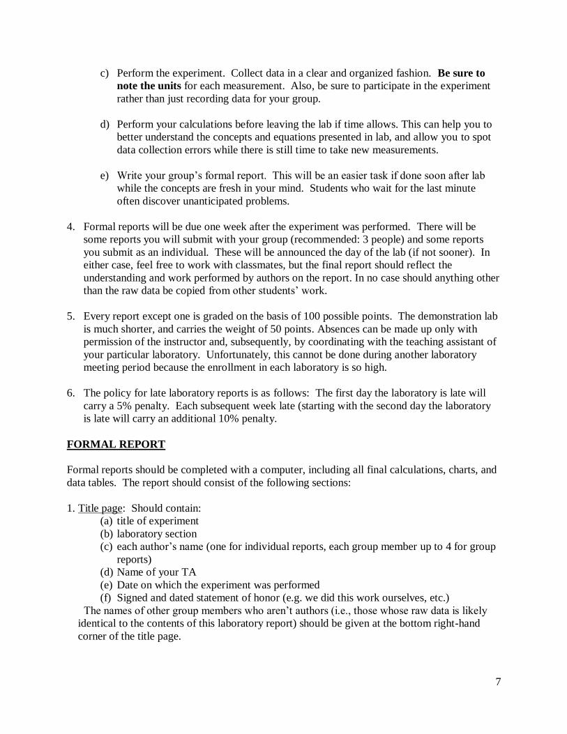
SPECIFIC GRAVITY (Crowe et al., Ch. 2.1)
Figure 1: Hydrometer
gρ
γ
γ
ρ
ρ
water
fluid
water
fluid
Volume
Weight )(Weight Specific
Volume
Mass )(Density
(s)Gravity Specific
10
Procedure:
A. Hydrometers
Two selected fluids have been placed in glass containers together with hydrometers. The liquids
used in these tests are among those listed in table A-4.
1. Take readings for both fluids. The scales read from the top down, and the readings must
be divided by 1000 to obtain the specific gravity. The hydrometer should not be touching
the sides of the container.
2. Calculate the specific weight () and the density () in both SI units (N/m3 and kg/m
3) and
English units (lb/ft3 and slugs/ft
3). Tentatively identify the two fluids in table A-4.
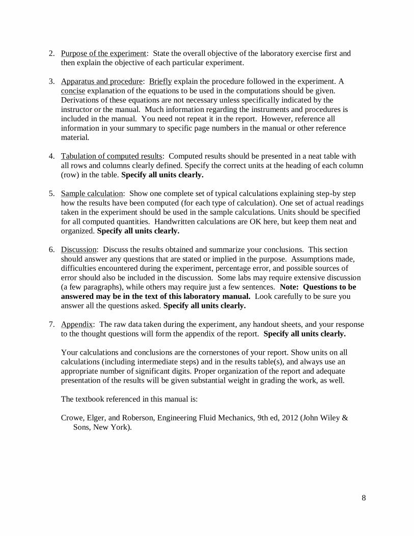
Figure 2: Westphal Balance
B. Westphal Balance:
Use the Westphal Balance to obtain the specific gravity of Sigma-Aldrich Mineral Oil. Collect
all the readings from the class and determine the mean and the standard deviation of the
readings.
1. Check that the instrument is balanced.
2. Release the balance beam by turning the knob in the middle of the base.
3. Check that the glass plummet is not touching the sides of the container.
4. Adjust the metal weight on top and the weighted chain (using the knob on the left side)
until the indicator is centered (on the scale at the bottom).
5. Read the specific gravity of the fluid. Read to 4 decimal places - the weighted chain uses
a vernier scale.
6. Return the metal weight to the center and move the weighted chain back to the bottom of
the scale.
7. Lock the balance beam.
8. Collect the values from all of the groups and calculate the mean and standard deviation.
Calculate and in SI and English units. Compare your values to the ones listed in the
table and calculate %error.
11
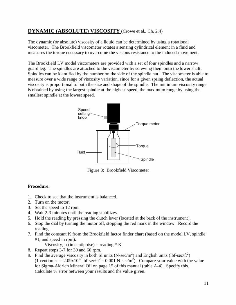
DYNAMIC (ABSOLUTE) VISCOSITY (Crowe et al., Ch. 2.4)
The dynamic (or absolute) viscosity of a liquid can be determined by using a rotational
viscometer. The Brookfield viscometer rotates a sensing cylindrical element in a fluid and
measures the torque necessary to overcome the viscous resistance to the induced movement.
The Brookfield LV model viscometers are provided with a set of four spindles and a narrow
guard leg. The spindles are attached to the viscometer by screwing them onto the lower shaft.
Spindles can be identified by the number on the side of the spindle nut. The viscometer is able to
measure over a wide range of viscosity variation, since for a given spring deflection, the actual
viscosity is proportional to both the size and shape of the spindle. The minimum viscosity range
is obtained by using the largest spindle at the highest speed, the maximum range by using the
smallest spindle at the lowest speed.
Figure 3: Brookfield Viscometer
Procedure:
1. Check to see that the instrument is balanced.
2. Turn on the motor.
3. Set the speed to 12 rpm.
4. Wait 2-3 minutes until the reading stabilizes.
5. Hold the reading by pressing the clutch lever (located at the back of the instrument).
6. Stop the dial by turning the motor off, stopping the red mark in the window. Record the
reading.
7. Find the constant K from the Brookfield factor finder chart (based on the model LV, spindle
#1, and speed in rpm).
Viscosity, µ (in centipoise) = reading * K
8. Repeat steps 3-7 for 30 and 60 rpm.
9. Find the average viscosity in both SI units (N-sec/m2) and English units (lbf-sec/ft
2)
(1 centipoise = 2.09x10⁻⁵
lbf-sec/ft2
= 0.001 N-sec/m2). Compare your value with the value
for Sigma-Aldrich Mineral Oil on page 15 of this manual (table A-4). Specify this.
Calculate % error between your results and the value given.
12
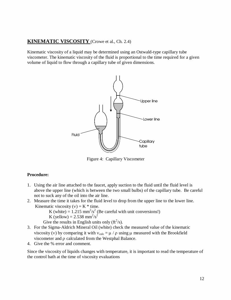
KINEMATIC VISCOSITY (Crowe et al., Ch. 2.4)
Kinematic viscosity of a liquid may be determined using an Ostwald-type capillary tube
viscometer. The kinematic viscosity of the fluid is proportional to the time required for a given
volume of liquid to flow through a capillary tube of given dimensions.
Figure 4: Capillary Viscometer
Procedure:
1. Using the air line attached to the faucet, apply suction to the fluid until the fluid level is
above the upper line (which is between the two small bulbs) of the capillary tube. Be careful
not to suck any of the oil into the air line.
2. Measure the time it takes for the fluid level to drop from the upper line to the lower line.
Kinematic viscosity () = K * time.
K (white) = 1.215 mm2/s
2 (Be careful with unit conversions!)
K (yellow) = 2.538 mm2/s
2
Give the results in English units only (ft2/s).
3. For the Sigma-Aldrich Mineral Oil (white) check the measured value of the kinematic
viscosity () by comparing it with calc = / using measured with the Brookfield
viscometer and calculated from the Westphal Balance.
4. Give the % error and comment.
Since the viscosity of liquids changes with temperature, it is important to read the temperature of
the control bath at the time of viscosity evaluations
13
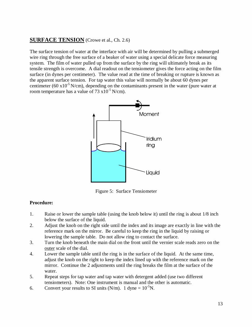
SURFACE TENSION (Crowe et al., Ch. 2.6)
The surface tension of water at the interface with air will be determined by pulling a submerged
wire ring through the free surface of a beaker of water using a special delicate force measuring
system. The film of water pulled up from the surface by the ring will ultimately break as its
tensile strength is overcome. A dial readout on the tensiometer gives the force acting on the film
surface (in dynes per centimeter). The value read at the time of breaking or rupture is known as
the apparent surface tension. For tap water this value will normally be about 60 dynes per
centimeter (60 x10-5
N/cm), depending on the contaminants present in the water (pure water at
room temperature has a value of 73 x10-5
N/cm).
Figure 5: Surface Tensiometer
Procedure:
1. Raise or lower the sample table (using the knob below it) until the ring is about 1/8 inch
below the surface of the liquid.
2. Adjust the knob on the right side until the index and its image are exactly in line with the
reference mark on the mirror. Be careful to keep the ring in the liquid by raising or
lowering the sample table. Do not allow ring to contact the surface.
3. Turn the knob beneath the main dial on the front until the vernier scale reads zero on the
outer scale of the dial.
4. Lower the sample table until the ring is in the surface of the liquid. At the same time,
adjust the knob on the right to keep the index lined up with the reference mark on the
mirror. Continue the 2 adjustments until the ring breaks the film at the surface of the
water.
5. Repeat steps for tap water and tap water with detergent added (use two different
tensiometers). Note: One instrument is manual and the other is automatic.
6. Convert your results to SI units (N/m). 1 dyne = 10-5
N.
14
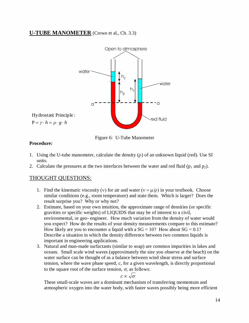
U-TUBE MANOMETER (Crowe et al., Ch. 3.3)
Figure 6: U-Tube Manometer
Procedure:
1. Using the U-tube manometer, calculate the density () of an unknown liquid (red). Use SI
units.
2. Calculate the pressures at the two interfaces between the water and red fluid (p1 and p2).
THOUGHT QUESTIONS:
1. Find the kinematic viscosity ( for air and water ( in your textbook. Choose
similar conditions (e.g., room temperature) and state them. Which is larger? Does the
result surprise you? Why or why not?
2. Estimate, based on your own intuition, the approximate range of densities (or specific
gravities or specific weights) of LIQUIDS that may be of interest to a civil,
environmental, or geo- engineer. How much variation from the density of water would
you expect? How do the results of your density measurements compare to this estimate?
How likely are you to encounter a liquid with a SG = 10? How about SG = 0.1?
Describe a situation in which the density difference between two common liquids is
important in engineering applications.
3. Natural and man-made surfactants (similar to soap) are common impurities in lakes and
oceans. Small scale wind waves (approximately the size you observe at the beach) on the
water surface can be thought of as a balance between wind shear stress and surface
tension, where the wave phase speed, c, for a given wavelength, is directly proportional
to the square root of the surface tension, , as follows:
c
These small-scale waves are a dominant mechanism of transferring momentum and
atmospheric oxygen into the water body, with faster waves possibly being more efficient
hgρh P
: PrinciplecHydrostati
15
than slower waves for facilitating these generally desirable processes. Based on the
results you obtained in lab, describe qualitatively how surfactants on the surface of the
water body (i.e. “surface slicks”) will affect the transport of momentum and oxygen into
the water body.
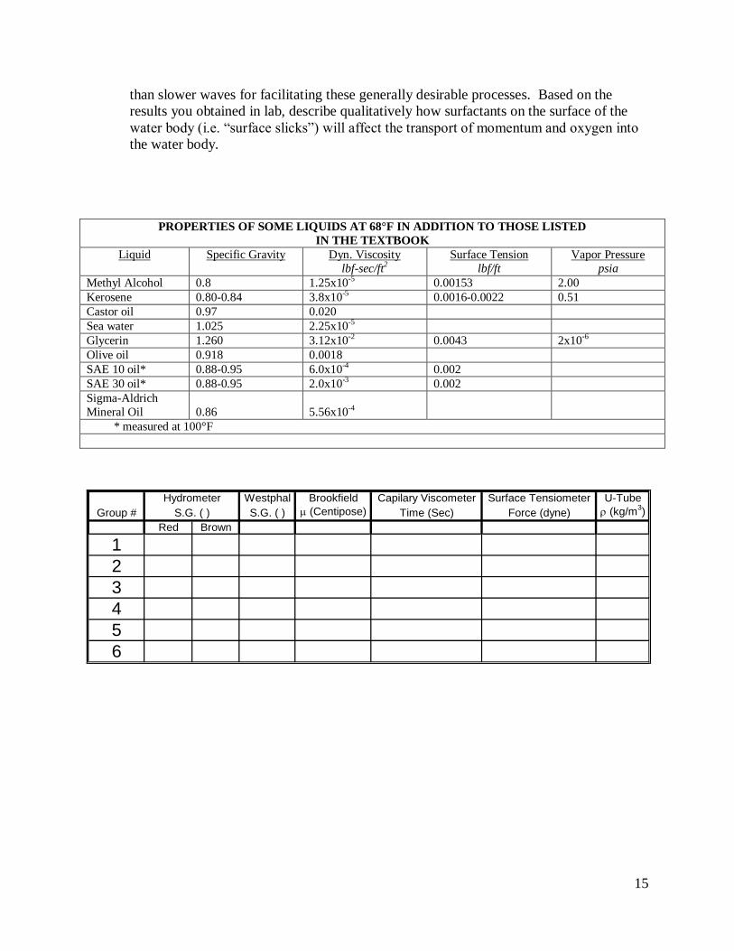
PROPERTIES OF SOME LIQUIDS AT 68°F IN ADDITION TO THOSE LISTED
IN THE TEXTBOOK
Liquid Specific Gravity Dyn. Viscosity
lbf-sec/ft2 Surface Tension
lbf/ft
Vapor Pressure
psia
Methyl Alcohol 0.8 1.25x10⁻⁵ 0.00153 2.00
Kerosene 0.80-0.84 3.8x10⁻⁵ 0.0016-0.0022 0.51
Castor oil 0.97 0.020
Sea water 1.025 2.25x10⁻⁵
Glycerin 1.260 3.12x10⁻² 0.0043 2x10⁻⁶
Olive oil 0.918 0.0018
SAE 10 oil* 0.88-0.95 6.0x10⁻⁴ 0.002
SAE 30 oil* 0.88-0.95 2.0x10⁻³ 0.002
Sigma-Aldrich
Mineral Oil
0.86
5.56x10⁻⁴
* measured at 100°F
Westphal Brookfield Capilary Viscometer Surface Tensiometer U-Tube
Group # S.G. ( ) (Centipose) Time (Sec) Force (dyne) (kg/m3)
Red Brown
1
2
3
4
5
6
Hydrometer
S.G. ( )
16
CE 3502 FLUID MECHANICS
Laboratory Experiment #2
PRESSURE & VELOCITY MEASUREMENT
Measuring the pressure at a point in a flow field is one of the most common engineering fluid
mechanics problems. Laboratories frequently use U-tube manometers, piezometric tubes, or
pressure gages for measuring relatively steady pressures. When time-dependent (unsteady)
pressures have to be recorded, it is recommended to use electronic pressure transducers, which
are highly responsive to pressure oscillations.
Closely related to pressure measurements are velocity measurements. Both are used to describe a
flow field. The velocity at a point in a fluid stream may be measured by several methods. The
most commonly used are the stagnation tube, Pitot tube, and the current meter. There are also
some more delicate devices such as hot wires, Laser-Doppler systems (LDA) and particle image
velocimetry (PIV). Additional information for some of these devices can be found in the
textbook, Chapters 4 and 6. If you want additional information, please ask your instructors.
In order to demonstrate how the velocity profile in a flow can be measured and used to determine
volumetric discharge, an experiment will be performed using stagnation tubes in an air stream
flowing through a pipe. A two-inch diameter pipe has been fitted with a rake of stagnation tubes
and a static pressure tap on the pipe wall. These are connected to a manometer bank filled with
colored water, which will be used to determine a local velocity at the location of each stagnation
tube within the cross-section of the pipe. The mean velocity is calculated from these local
velocities by integrating a plot of local velocity vs. the square of the radial coordinate. This
velocity is then compared with velocities determined using two additional approaches.
The two other measurements of flow velocity are obtained from (1) a Hastings meter and (2) a
Venturi meter, which is a constricted section of the pipe with known geometry. A manometer
connected to two static pressure taps on the Venturi meter (one at the constriction and one just
upstream of it) is used to determine the pressure loss through the constriction, which can be
related to the flow rate using a calibrated equation. Both measurements are described in more
detail in the procedure section.
17
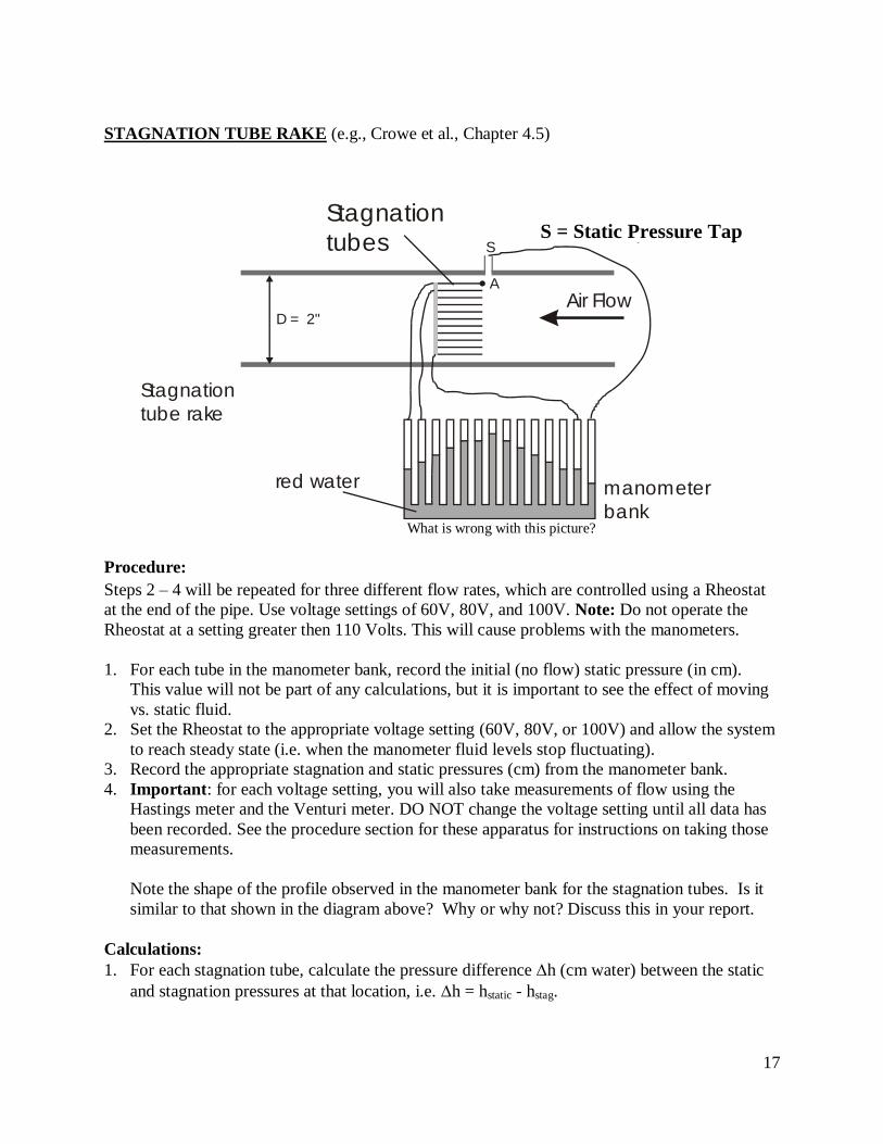
STAGNATION TUBE RAKE (e.g., Crowe et al., Chapter 4.5)
SS = static pressure tap
Air FlowD = 2"
Stagnation
tube rake
A
Stagnation
tubes
red water manometer
bank What is wrong with this picture?
Procedure:
Steps 2 – 4 will be repeated for three different flow rates, which are controlled using a Rheostat
at the end of the pipe. Use voltage settings of 60V, 80V, and 100V. Note: Do not operate the
Rheostat at a setting greater then 110 Volts. This will cause problems with the manometers.
1. For each tube in the manometer bank, record the initial (no flow) static pressure (in cm).
This value will not be part of any calculations, but it is important to see the effect of moving
vs. static fluid.
2. Set the Rheostat to the appropriate voltage setting (60V, 80V, or 100V) and allow the system
to reach steady state (i.e. when the manometer fluid levels stop fluctuating).
3. Record the appropriate stagnation and static pressures (cm) from the manometer bank.
4. Important: for each voltage setting, you will also take measurements of flow using the
Hastings meter and the Venturi meter. DO NOT change the voltage setting until all data has
been recorded. See the procedure section for these apparatus for instructions on taking those
measurements.
Note the shape of the profile observed in the manometer bank for the stagnation tubes. Is it
similar to that shown in the diagram above? Why or why not? Discuss this in your report.
Calculations:
1. For each stagnation tube, calculate the pressure difference h (cm water) between the static
and stagnation pressures at that location, i.e. h = hstatic - hstag.
S = Static Pressure Tap
18
2. Calculate the local velocities at each stagnation tube fromair
whgu
2 . This can be
derived from the Bernoulli equation, which will be discussed in the near future.
Check your units to make sure the result is dimensionally consistent and reasonable!!!
3. Plot the velocity distribution, u(r) vs. r, where r is the radial location of the tube (distance
from the center of the pipe).
4. Discuss the shape of the velocity profile as a consequence of viscous wall shear stress.
5. Plot u(r) vs. r2.
6. Find the volumetric flow rate Q by numerical or graphical integration of the area under the
u(r) vs. r2 curve (multiply this area by ). Show in your report why this integration yields the
volumetric flow rate within the pipe. Hint: refer to the calculus concept of finding volume
under the surface generated by rotation of a curve about an axis.
7. Calculate the mean velocity of flow in the cross section: V = Q/A
8. Determine which of the stagnation tubes in the rake most nearly measures the mean velocity
9. Repeat these calculations (Steps 1 – 8) for the second and third flow rates.
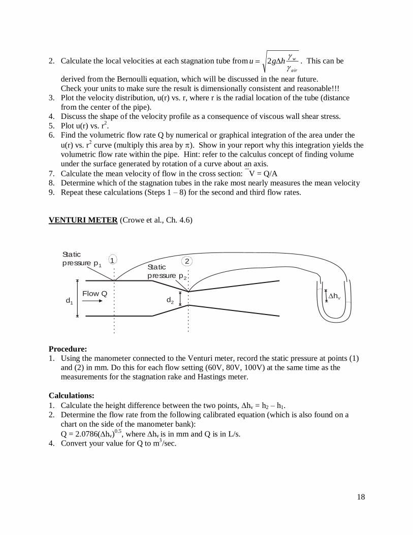
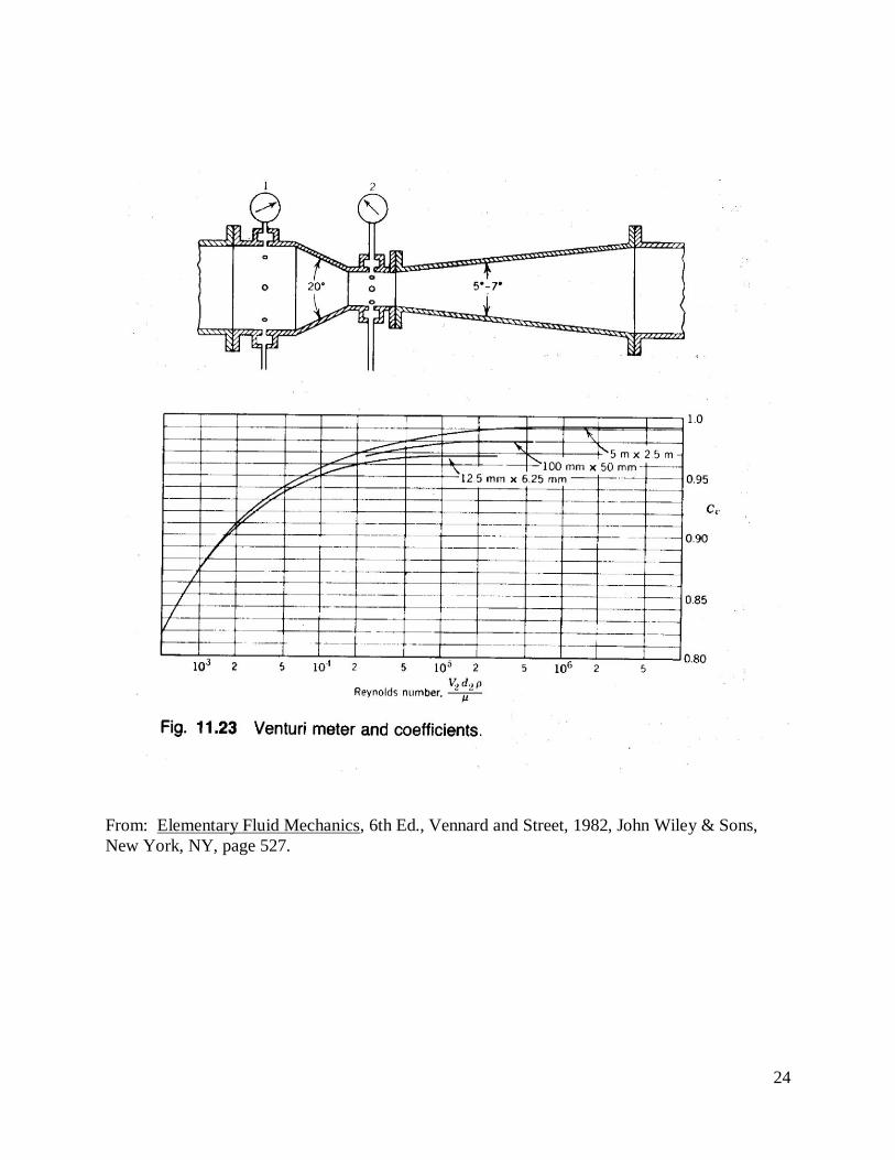
VENTURI METER (Crowe et al., Ch. 4.6)
d1d2
1 2
hVFlow Q
Static
pressure p1 Static
pressure p2
Procedure:
1. Using the manometer connected to the Venturi meter, record the static pressure at points (1)
and (2) in mm. Do this for each flow setting (60V, 80V, 100V) at the same time as the
measurements for the stagnation rake and Hastings meter.
Calculations:
1. Calculate the height difference between the two points, hv = h2 – h1.
2. Determine the flow rate from the following calibrated equation (which is also found on a
chart on the side of the manometer bank):
Q = 2.0786(hv)0.5
, where hv is in mm and Q is in L/s.
4. Convert your value for Q to m3/sec.
19
HASTINGS METER
Procedure:
1. Record the flow rate Q (in m3/min) directly from the Hastings meter. Note that a reading of
123 = 1.23 m3/min. Do this for each flow setting (60V, 80V, 100V) at the same time as the
measurements for the stagnation rake and the Venturi meter.
Calculations:
1. Convert your reading to m3/sec.
2. Calculate: Hastings
Venturi
Q
QK
This is the correction factor for the Hastings meter. Save this value as it will be used in
future labs.
3. For each voltage setting, compare the flow rates determined from the three methods in this
experiment (stagnation rake, Venturi meter, and Hastings meter). Which method do you
think is the most accurate? Why? What are some potential sources of error in these
measurements?
THOUGHT QUESTIONS: 1. Before performing the experiment, estimate a reasonable average air velocity for the
pipes used in this lab. Is it 1 m/s? 10 m/s? 100 m/s? 1000 m/s? More? Somewhere
in between? Convert to more familiar units (e.g. miles per hour) if you have trouble
estimating speeds in SI units. In a 2-inch diameter pipe, what flow rate corresponds
to your estimated velocity? The average student apartment in the Twin Cities has less
than 1000 ft2 of finished space (usually MUCH less). Assuming 8-foot ceilings (or
10-foot if you like round numbers), estimate the time required to fill the average
student apartment with a fluid at the flow rate you estimated for the air pipes
previously. How long would it take to fill a five-gallon bucket? Does your result
seem reasonable? Is your estimated flow rate substantially different (on an order of
magnitude basis) from the results obtained during the experiment? If so, is the
discrepancy a result of a misestimate or a miscalculation?
20
CE 3502 FLUID MECHANICS
Laboratory Experiment #3
APPLICATIONS OF THE BERNOULLI EQUATION
The Bernoulli Equation for steady, incompressible, inviscid flow along a streamline is given in
Sec. 4.5 of your textbook. Some illustrations of its use, particularly in flow measurement, are
also presented in Chapter 4. The Bernoulli equation for irrotational flow is derived in Chapter
4.7 of the textbook. Its applications are also discussed.
EXPERIMENT
The experiment deals with the measurement of discharge in several flows by measuring a
pressure difference and applying the Bernoulli equation and the equation of continuity to
calculate the discharge. A comparison will be made between the values calculated from
Bernoulli (‘ideal’ flow) and those obtained experimentally through the use of a previously
calibrated device (‘real’ flow). You will be assigned three types of flow meters for your
experiment: a Venturi meter, an orifice meter, and a sluice gate.
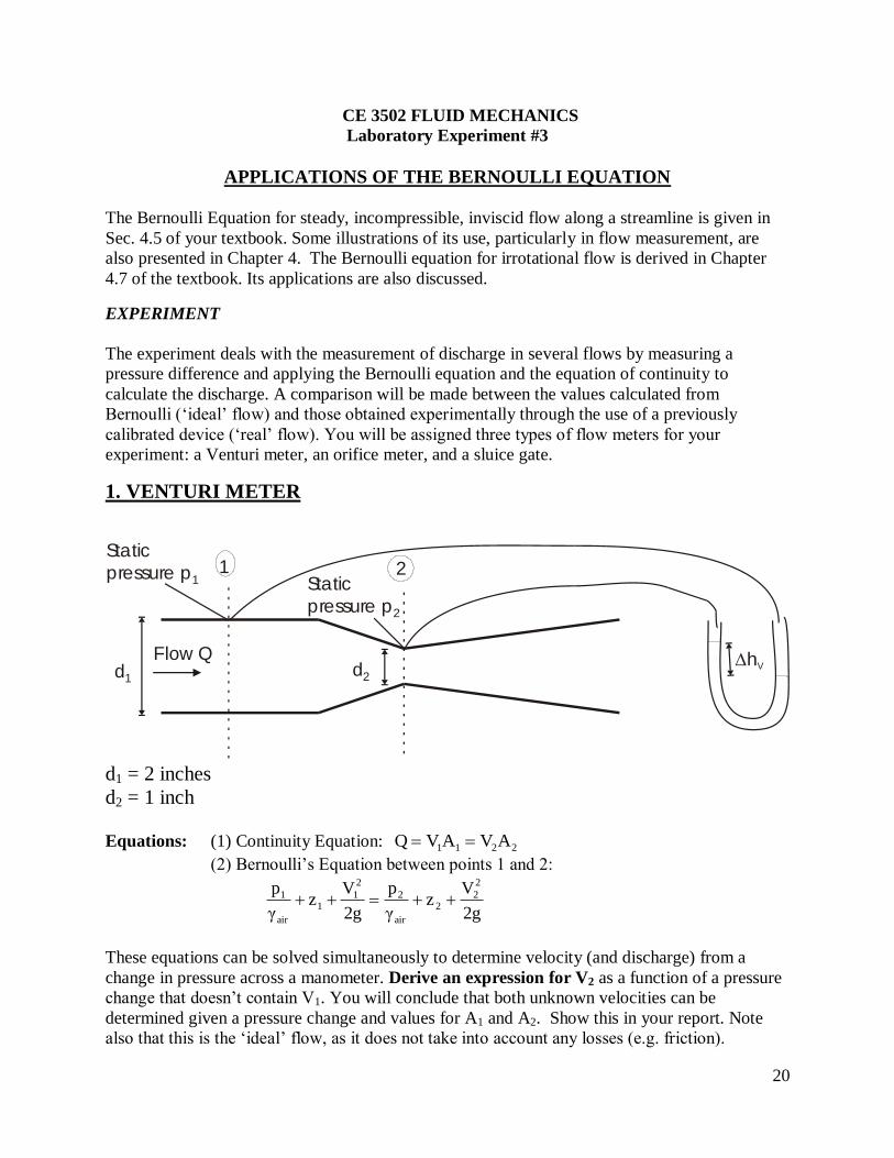
1. VENTURI METER
d1d2
1 2
hVFlow Q
Static
pressure p1 Static
pressure p2
d1 = 2 inches
d2 = 1 inch
Equations: (1) Continuity Equation: 2211 AVAVQ
(2) Bernoulli’s Equation between points 1 and 2:
2g
Vz
γ
p
2g
Vz
γ
p 2
22
air
2
2
11
air
1
These equations can be solved simultaneously to determine velocity (and discharge) from a
change in pressure across a manometer. Derive an expression for V2 as a function of a pressure
change that doesn’t contain V1. You will conclude that both unknown velocities can be
determined given a pressure change and values for A1 and A2. Show this in your report. Note
also that this is the ‘ideal’ flow, as it does not take into account any losses (e.g. friction).
21
Procedure:
Use Pipe 1 or Pipe 2. For three different speeds (60, 80, 100 Volt settings on the rheostat):
1. Measure hv from the large manometer bank for the Venturi Meter. This will be used
to determine the ideal flow rate, Qideal.
2. Measure hmean from the stagnation tube rake; this is the difference in pressure
between the static tap and a stagnation tube assumed to correspond to the mean
velocity. This will be used to find the mean (real) velocity and flow rate, Qreal.
hmean = hstatic – hr, where hr is read from the stagnation tube at r = 0.85” for pipe #1
and r = 0.75” for pipe #2
If your data from Lab #2 showed that a different radius matched the mean velocity,
then use that radius instead of the one above.
3. Read the flow rate from the Hastings electronic flow meter. This provides a second
measurement of Qreal.
Qreal = QHastings*Km3
min
æ
èç
ö
ø÷
where K is the correction factor computed in Lab #2 or given by the instructor.
Calculations:
Part 1:
1. Calculate the pressure loss through the Venturi meter, p = w hv
2. Calculate Qideal by using p in the equation for Videal that you derived from the
Bernoulli and continuity equations (Qideal = V2,ideal*A2 = V1,ideal*A1). Do NOT use the
equation from the side of the manometer bank, it is a calibrated equation.
3. Calculate Qreal from Qreal = Vreal*A. Vreal is the mean velocity calculated by using
hmean in the equation for the local velocity u at a point in the stagnation rake (see
previous lab).
4. Calculate the discharge correction coefficient. ideal
realV
Q
QC
5. Calculate the Reynolds number for pipe flow measured at the throat of the Venturi
meter.
air
dV
22Re where air is the kinematic viscosity of air, and
2
real
2A
Qv
6. Plot your results on the graph on page 24.
Part 2:
1. Using Qreal from the Hastings meter, calculate the discharge correction coefficient:
ideal
realV
Q
QC
2. Calculate the corresponding Reynolds number.
3. Plot your results on the same copy of the graph on page 24.
Why is Qreal different than Qideal? Which is greater? Why? Address this in the discussion section
of your report.
22
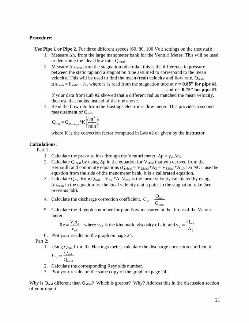
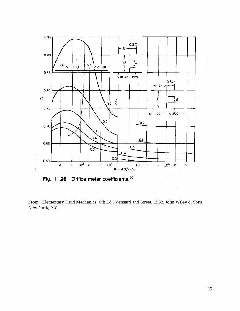
2. ORIFICE METER (e.g., examples in Chapter 13.2 and 13.4)
d1 d2
hFlow d = 2”
d = 1.5”1
2
static
pressure p1
Static
pressure p2
1 2
The contraction coefficient for this set-up is:
2
1
2C
A
A0.40.6C
Procedure:
Use Pipe 3. For three different speeds (60, 80, 100 Volt settings on the rheostat):
1. Measure ho from the manometer connected to the orifice meter. This will be used to
find Qideal using the equations given below.
2. Get Qreal from the Hastings Mass Flow Meter:
e.g. Qreal = QHastings*K m3
min where K is the correction factor (1.1180)
Calculations:
1. Calculate Qideal using the orifice equation Q =CCA2
1- CC
2 A2
A1
æ
èç
ö
ø÷
22g(Dho )
gwatergair
2. Calculate the discharge correction coefficient ideal
realV
Q
QC
3. Calculate the Reynolds number
4. Plot C vs. Re on Figure 11.26 on page 23, using 2
1
22
C
CV
A
AC1
CCC

23
3. SLUICE GATE (Crowe et al., Ch. 6.4)
Prandtl Tube y 1
y 3 V 2
h
y 2
V 1
Gate
1
2
*The Prandtl tube measures both stagnation pressure and static pressure. It has separate pressure
taps and separate outlets for each. Look at the Prandtl tube to locate the pressure taps.
Procedure:
1. Measure y1 and y2. These will be used to determine the ideal flow rate, qideal.
2. Measure h from the Prandtl tube manometer, this will be used to find the mean velocity
Calculations:
1. Calculate qideal (flow per unit width) using the Bernoulli and continuity equations applied
to the sluice gate.
2. Using h from the Prandtl tube manometer, calculate the mean (real) velocity
downstream of the sluice gate: V = 2gDh. Then qreal =V * y2
3. Calculate CV =qreal
qideal
THOUGHT QUESTIONS: 1. Explain the difference between static and stagnation pressure. Which is larger? And by
how much? Why? Hint: consider a force balance on a small element of fluid along the
pipe wall and on a small element of fluid just upstream of a stagnation tube.
2. As you’ve seen, static pressures increase with decreasing velocity. Qualitatively describe
how this principle explains how an airplane wing generates lift. How might such an
analysis be useful in designing certain types of hydraulic structures where the long-term
effects of static pressure differences may cause damage and/or failure of the structure?
Such problems can be minimized by proper consideration of the flow properties or by
overly strengthening the structures. Which approach is most desirable from the
standpoint of safety? From the standpoint of cost? From the standpoint of long-term
durability and maintenance concerns? Why?
3. Given your experience with flow acceleration through the throat of a Venturi meter and
under a sluice gate, consider an atmospheric flow over a hill where the flow far above the
hill is not affected by the hill. How might such an analysis be useful in designing hilltop
structures that are sensitive to wind forces? How might a continuity analysis be useful in
considering wind acceleration between the large buildings in downtown Minneapolis?
Describe safety concerns with such a deflection of atmospheric flows in an urban area.
24
From: Elementary Fluid Mechanics, 6th Ed., Vennard and Street, 1982, John Wiley & Sons,
New York, NY, page 527.
25
From: Elementary Fluid Mechanics, 6th Ed., Vennard and Street, 1982, John Wiley & Sons,
New York, NY.
26
CE 3502 FLUID MECHANICS
Laboratory Experiment #4
APPLICATIONS OF THE MOMENTUM THEOREM
The momentum theorem states that the rate of change in momentum of a fluid “particle” or
control volume is equal to the sum of the forces on the fluid. This principle and its resulting
equations may be used to determine the fluid accelerations where the external forces are known.
Conversely, if the accelerations are known beforehand, the applied forces may be determined for
design purposes.
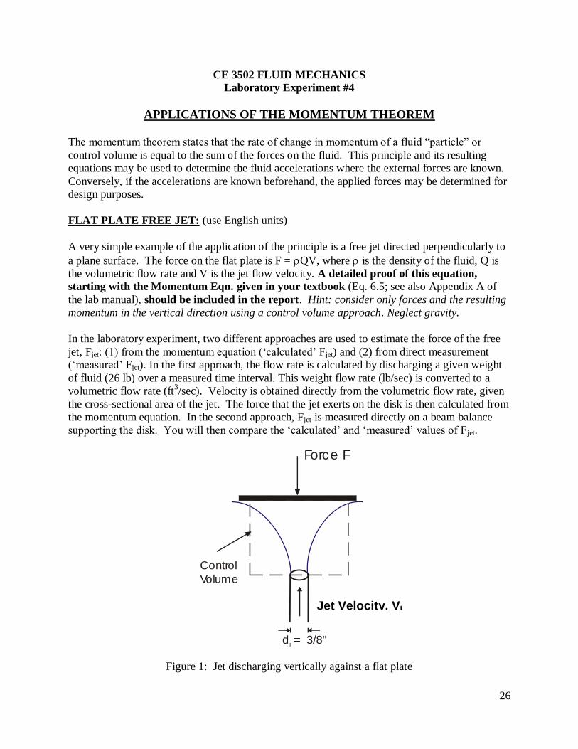
FLAT PLATE FREE JET: (use English units)
A very simple example of the application of the principle is a free jet directed perpendicularly to
a plane surface. The force on the flat plate is F = QV, where is the density of the fluid, Q is
the volumetric flow rate and V is the jet flow velocity. A detailed proof of this equation,
starting with the Momentum Eqn. given in your textbook (Eq. 6.5; see also Appendix A of
the lab manual), should be included in the report. Hint: consider only forces and the resulting
momentum in the vertical direction using a control volume approach. Neglect gravity.
In the laboratory experiment, two different approaches are used to estimate the force of the free
jet, Fjet: (1) from the momentum equation (‘calculated’ Fjet) and (2) from direct measurement
(‘measured’ Fjet). In the first approach, the flow rate is calculated by discharging a given weight
of fluid (26 lb) over a measured time interval. This weight flow rate (lb/sec) is converted to a
volumetric flow rate (ft3/sec). Velocity is obtained directly from the volumetric flow rate, given
the cross-sectional area of the jet. The force that the jet exerts on the disk is then calculated from
the momentum equation. In the second approach, Fjet is measured directly on a beam balance
supporting the disk. You will then compare the ‘calculated’ and ‘measured’ values of Fjet.
d = 3/8"j
Control
Volume
Force F
Jet velocity Vj
Figure 1: Jet discharging vertically against a flat plate
Jet Velocity, Vj
27
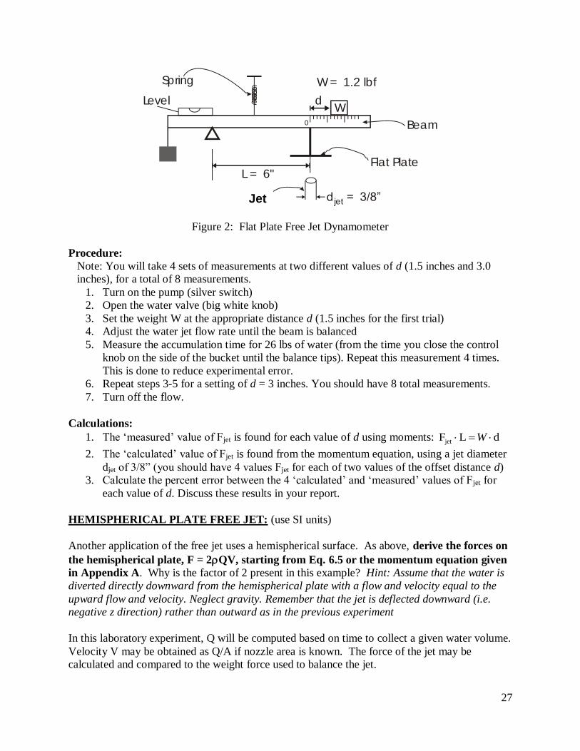
Spring
Beam
Jet
W0
L = 6"
W = 1.2 lbf
Flat Plate
d
d = 3/8”jet
Level
Figure 2: Flat Plate Free Jet Dynamometer
Procedure:
Note: You will take 4 sets of measurements at two different values of d (1.5 inches and 3.0
inches), for a total of 8 measurements.
1. Turn on the pump (silver switch)
2. Open the water valve (big white knob)
3. Set the weight W at the appropriate distance d (1.5 inches for the first trial)
4. Adjust the water jet flow rate until the beam is balanced
5. Measure the accumulation time for 26 lbs of water (from the time you close the control
knob on the side of the bucket until the balance tips). Repeat this measurement 4 times.
This is done to reduce experimental error.
6. Repeat steps 3-5 for a setting of d = 3 inches. You should have 8 total measurements.
7. Turn off the flow.
Calculations:
1. The ‘measured’ value of Fjet is found for each value of d using moments: dLFjet W
2. The ‘calculated’ value of Fjet is found from the momentum equation, using a jet diameter
djet of 3/8” (you should have 4 values Fjet for each of two values of the offset distance d)
3. Calculate the percent error between the 4 ‘calculated’ and ‘measured’ values of Fjet for
each value of d. Discuss these results in your report.
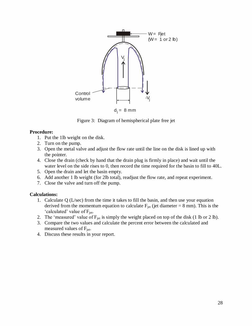
HEMISPHERICAL PLATE FREE JET: (use SI units)
Another application of the free jet uses a hemispherical surface. As above, derive the forces on
the hemispherical plate, F = 2QV, starting from Eq. 6.5 or the momentum equation given
in Appendix A. Why is the factor of 2 present in this example? Hint: Assume that the water is
diverted directly downward from the hemispherical plate with a flow and velocity equal to the
upward flow and velocity. Neglect gravity. Remember that the jet is deflected downward (i.e.
negative z direction) rather than outward as in the previous experiment
In this laboratory experiment, Q will be computed based on time to collect a given water volume.
Velocity V may be obtained as Q/A if nozzle area is known. The force of the jet may be
calculated and compared to the weight force used to balance the jet.
Jet
28
d = 8 mmj
Vj
-Vj
Control
volume
W = Fjet
(W = 1 or 2 lb)
Figure 3: Diagram of hemispherical plate free jet
Procedure:
1. Put the 1lb weight on the disk.
2. Turn on the pump.
3. Open the metal valve and adjust the flow rate until the line on the disk is lined up with
the pointer.
4. Close the drain (check by hand that the drain plug is firmly in place) and wait until the
water level on the side rises to 0, then record the time required for the basin to fill to 40L.
5. Open the drain and let the basin empty.
6. Add another 1 lb weight (for 2lb total), readjust the flow rate, and repeat experiment.
7. Close the valve and turn off the pump.
Calculations:
1. Calculate Q (L/sec) from the time it takes to fill the basin, and then use your equation
derived from the momentum equation to calculate Fjet (jet diameter = 8 mm). This is the
‘calculated’ value of Fjet.
2. The ‘measured’ value of Fjet is simply the weight placed on top of the disk (1 lb or 2 lb).
3. Compare the two values and calculate the percent error between the calculated and
measured values of Fjet.
4. Discuss these results in your report.
29
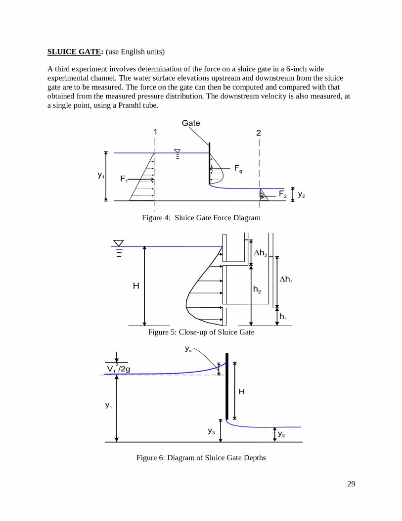
SLUICE GATE: (use English units)
A third experiment involves determination of the force on a sluice gate in a 6-inch wide
experimental channel. The water surface elevations upstream and downstream from the sluice
gate are to be measured. The force on the gate can then be computed and compared with that
obtained from the measured pressure distribution. The downstream velocity is also measured, at
a single point, using a Prandtl tube.
Figure 4: Sluice Gate Force Diagram
Figure 5: Close-up of Sluice Gate
Figure 6: Diagram of Sluice Gate Depths
30
Procedure:
1. Measure y1, y2, y3, where y1 is the upstream flow depth, y2 is the downstream flow depth,
and y3 is the distance between channel bottom and gate bottom.
2. Measure h from the manometer connected to the Prandtl tube. This will be used to find
the flow velocity, V2.
3. Measure the static pressures along the gate’s surface using the manometers connected to
taps in the gate. You will record the height of the water in each tube. You will also need
to record the height of each tap above the bottom of the gate; this is obtained from a sheet
on the side of the sluice gate.
Calculations:
1. Velocity and flow calculations:
a. Calculate the downstream velocity using the Prandtl tube. hgV 22
b. Use V2 to calculate the flow rate. Q = V2 A2
Discuss possible errors in using this method of calculating Q.
c. Derive an equation for V2 using the Bernoulli and continuity equations
between sections 1 and 2 in Figure 4. Calculate and compare this velocity with
the measured value and give the percent error.
d. Discuss these results.
2. Force calculations:
a. From the momentum equation (Forces = Momentum) derive an expression
for the force on the gate and calculate F1 and F2. Solve for Fgate.
b. Calculate the static pressures along the gate’s surface. The pressure, P, at each tap
location is related to the height of water in the manometer using hydrostatic
principle (P = wh). Figure 5 illustrates the calculation of h for each tap.
c. Calculate Fgate using the pressure profile. Graph the pressure profile with p vs.
vertical distance h along the gate.
Assume pressure is zero at h = 0 and at h = H.
H = maximum wetted length = y1 + ys - y3, where ys = (V1)2 / 2g.
-- Assuming V1=0, then ys=0
Fgate is equal to the total area under the graph multiplied by the channel width.
(channel width = 6 inches)
d. Compare the two values of Fgate and give the percent error. Discuss the results.
THOUGHT QUESTIONS:
1. Consider the question about hydraulic structures in the previous section in terms of the
dynamic pressures/forces studied in this experiment. How can the shape and orientation
(with respect to the flow direction) of a hydraulic structure affect the forces that it is
required to bear?
2. Describe how such a momentum analysis should be implemented in the design of tall
buildings that are sensitive to wind stresses.
31
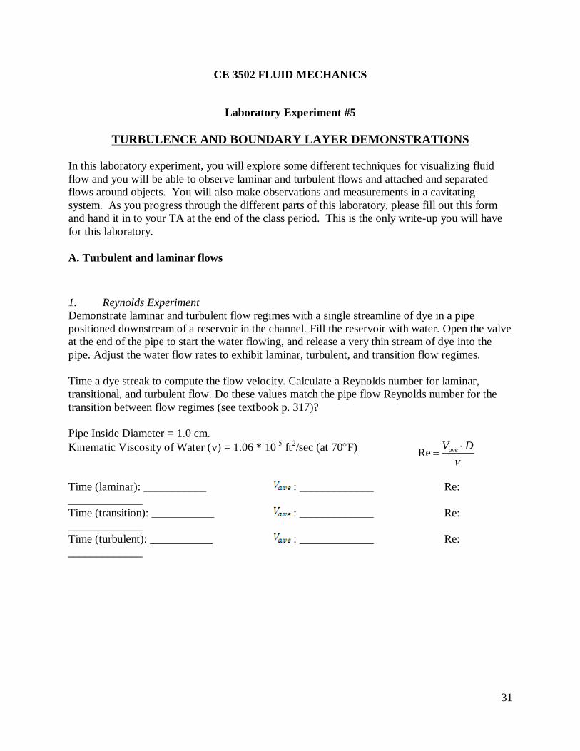
CE 3502 FLUID MECHANICS
Laboratory Experiment #5
TURBULENCE AND BOUNDARY LAYER DEMONSTRATIONS
In this laboratory experiment, you will explore some different techniques for visualizing fluid
flow and you will be able to observe laminar and turbulent flows and attached and separated
flows around objects. You will also make observations and measurements in a cavitating
system. As you progress through the different parts of this laboratory, please fill out this form
and hand it in to your TA at the end of the class period. This is the only write-up you will have
for this laboratory.
A. Turbulent and laminar flows
1. Reynolds Experiment
Demonstrate laminar and turbulent flow regimes with a single streamline of dye in a pipe
positioned downstream of a reservoir in the channel. Fill the reservoir with water. Open the valve
at the end of the pipe to start the water flowing, and release a very thin stream of dye into the
pipe. Adjust the water flow rates to exhibit laminar, turbulent, and transition flow regimes.
Time a dye streak to compute the flow velocity. Calculate a Reynolds number for laminar,
transitional, and turbulent flow. Do these values match the pipe flow Reynolds number for the
transition between flow regimes (see textbook p. 317)?
Pipe Inside Diameter = 1.0 cm.
Kinematic Viscosity of Water () = 1.06 * 10-5
ft2/sec (at 70F)
Time (laminar): ___________ : _____________ Re:
_____________
Time (transition): ___________ : _____________ Re:
_____________
Time (turbulent): ___________ : _____________ Re:
_____________
DVave Re
32
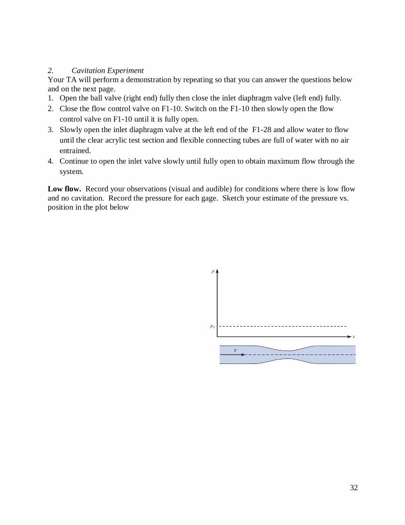
2. Cavitation Experiment
Your TA will perform a demonstration by repeating so that you can answer the questions below
and on the next page.
1. Open the ball valve (right end) fully then close the inlet diaphragm valve (left end) fully.
2. Close the flow control valve on F1-10. Switch on the F1-10 then slowly open the flow
control valve on F1-10 until it is fully open.
3. Slowly open the inlet diaphragm valve at the left end of the F1-28 and allow water to flow
until the clear acrylic test section and flexible connecting tubes are full of water with no air
entrained.
4. Continue to open the inlet valve slowly until fully open to obtain maximum flow through the
system.
Low flow. Record your observations (visual and audible) for conditions where there is low flow
and no cavitation. Record the pressure for each gage. Sketch your estimate of the pressure vs.
position in the plot below
33
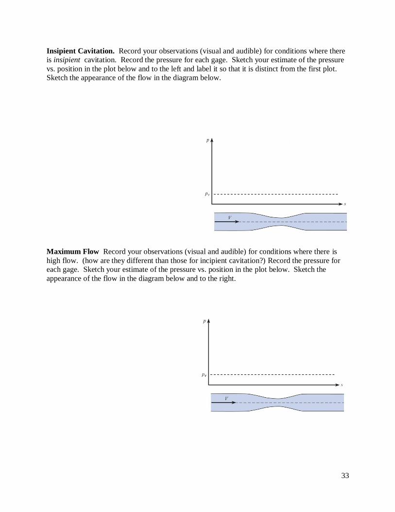
Insipient Cavitation. Record your observations (visual and audible) for conditions where there
is insipient cavitation. Record the pressure for each gage. Sketch your estimate of the pressure
vs. position in the plot below and to the left and label it so that it is distinct from the first plot.
Sketch the appearance of the flow in the diagram below.
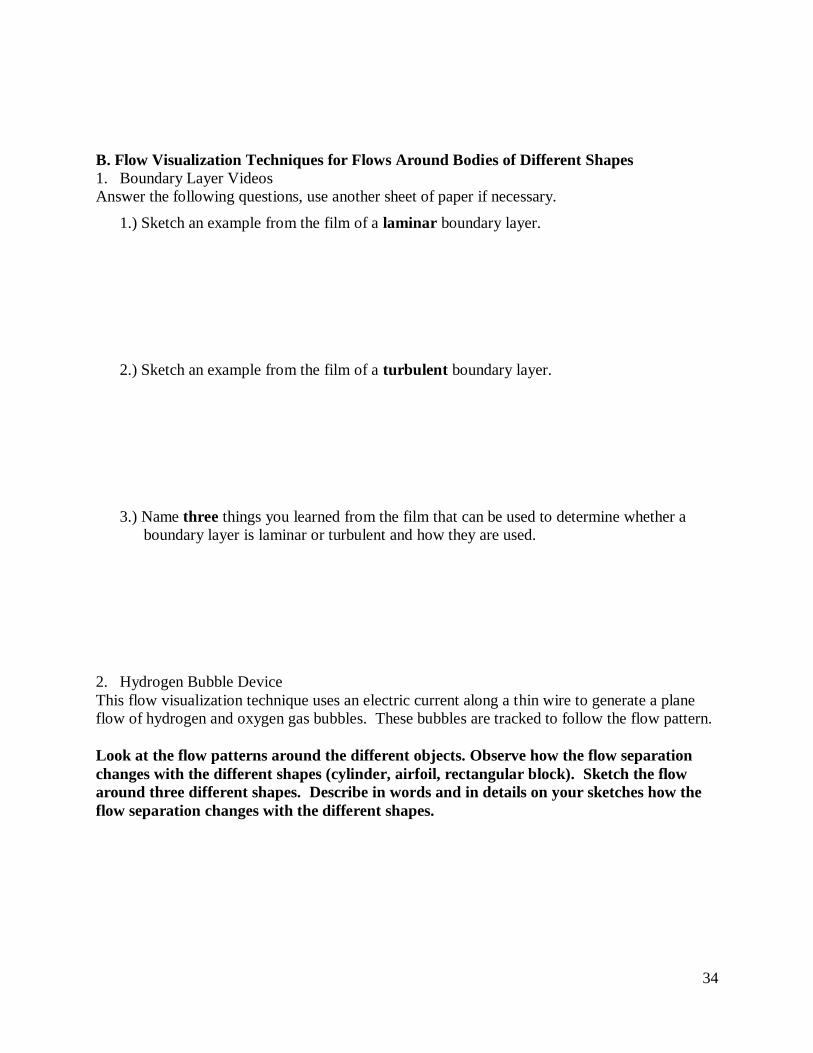
Maximum Flow Record your observations (visual and audible) for conditions where there is
high flow. (how are they different than those for incipient cavitation?) Record the pressure for
each gage. Sketch your estimate of the pressure vs. position in the plot below. Sketch the
appearance of the flow in the diagram below and to the right.
34
B. Flow Visualization Techniques for Flows Around Bodies of Different Shapes
1. Boundary Layer Videos
Answer the following questions, use another sheet of paper if necessary.
1.) Sketch an example from the film of a laminar boundary layer.
2.) Sketch an example from the film of a turbulent boundary layer.
3.) Name three things you learned from the film that can be used to determine whether a
boundary layer is laminar or turbulent and how they are used.
2. Hydrogen Bubble Device
This flow visualization technique uses an electric current along a thin wire to generate a plane
flow of hydrogen and oxygen gas bubbles. These bubbles are tracked to follow the flow pattern.
Look at the flow patterns around the different objects. Observe how the flow separation
changes with the different shapes (cylinder, airfoil, rectangular block). Sketch the flow
around three different shapes. Describe in words and in details on your sketches how the
flow separation changes with the different shapes.
35
CE 3502 FLUID MECHANICS
Laboratory Experiment #6
MEASUREMENTS OF PIPE FRICTION
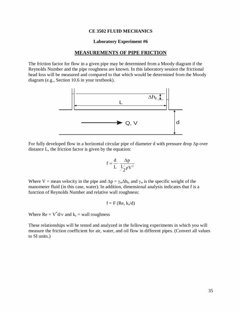
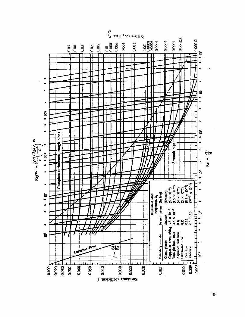
The friction factor for flow in a given pipe may be determined from a Moody diagram if the
Reynolds Number and the pipe roughness are known. In this laboratory session the frictional
head loss will be measured and compared to that which would be determined from the Moody
diagram (e.g., Section 10.6 in your textbook).
L
Q, V
hf
d
For fully developed flow in a horizontal circular pipe of diameter d with pressure drop p over
distance L, the friction factor is given by the equation:
2ρV2
1
Δp
L
d f
Where V = mean velocity in the pipe and p = whf, and w is the specific weight of the
manometer fluid (in this case, water). In addition, dimensional analysis indicates that f is a
function of Reynolds Number and relative wall roughness:
f = F (Re, ks/d)
Where Re = V*d/ and ks = wall roughness
These relationships will be tested and analyzed in the following experiments in which you will
measure the friction coefficient for air, water, and oil flow in different pipes. (Convert all values
to SI units.)
36
AIR FLOW (high Reynolds number flow)
A. Smooth Pipe (use pipe 3)
Procedure: For three fan speeds (60, 80, 100 Volt settings on the rheostat):
1. Measure the flow rate using the Hastings Meter with the appropriate correction factor
(k = 1.1180). Use this flow rate to calculate the velocity.
2. Measure the hf for two different lengths of pipe. Use a tape measure to measure these
lengths (L1 and L2).
Calculations:
1. Use hf to calculate p over the two different lengths of pipe (L1 and L2).
2. Calculate the friction coefficient (f) and the Reynolds number (Re) for each set of
measurements (6 total) and plot the points on the Moody Diagram.
3. Determine the equivalent sand roughness ks (in mm) for the pipe from these
measurements using the Moody Diagram.
B. Rough Pipe (use pipe 1 or 2)
Procedure:
For three fan speeds (60, 80, 100 Volt settings on the rheostat):
1. Measure the flow rate using the Venturi meter (use the equation from the side of the
manometer bank: Q = 2.0786(hv)0.5
where hv is in mm and Q is in L/s) and use it to
calculate the velocity.
2. Measure hf for two different lengths of pipe (L1 and L2), and measure these lengths with
the tape measure.
Calculations:
1. Use hf to calculate p over the two different lengths of pipe (L1 and L2).
2. Calculate the friction coefficient (f) and the Reynolds number (Re) for each set of
measurements (6 total) and plot the points on the Moody Diagram.
3. Determine the equivalent sand roughness ks (in mm) for the pipe from these
measurements using the Moody Diagram.
WATER FLOW
Procedure:
Using three different valve settings (1, 1.5, and 2 turns):
1. Measure Q: For the 1-inch diameter pipe, use the differential pressure gage connected to
the orifice meter to measure pressure drop pq (in psi) across the orifice plate.
2. Measure the pressure drop p over the length of pipe (in psi). Record the length between
the two points where the pressure taps are connected to the pipe (L = 10 ft).
Calculations:
1. Use pq in the orifice equation to find Q. Then use the flow rate (Q) to calculate the
velocity (V).
Q = 0.0535 (pq)1/2
(In this formula Q will be in ft3/s when p is in psi)
2. Calculate f and Re for each set of measurements (3 total) and plot the points on the
Moody Diagram. (A removable copy of the Moody Diagram in included in Appendix D.)
3. Determine the equivalent sand roughness ks (in mm) for the pipe.
37
THOUGHT QUESTIONS: 1. Based on the results from this lab and from the head loss equations, how would you
optimize pumping requirements for long pipelines that are required to discharge large
flows?
2. The friction factor for laminar flows, according to the moody Diagram, ranges from
0.025 to 0.1. For extremely turbulent flows, the friction factor is an order of magnitude
smaller. Why? Hint: think about what you know about the differences in velocity profile
shapes between laminar and turbulent flows – i.e. what effect do the differently shaped
boundary layers have of pipe friction factors?
38
39
CE FLUID MECHANICS
Laboratory Experiment #7
PIPE BENDS
In this part lab session, you will measure the energy loss coefficients for flow around 90º bends
in a copper pipe. There are three pipes. The first pipe is straight, and you will use measurements
from it to compute the friction coefficient for the copper pipe, as done in Lab 6, Pipe Friction.
The second pipe has one U-shaped loop in it (four 90º bends), and the third pipe has 2 loops in it
(eight 90º bends). Using the friction loss measured or calculated for the straight copper pipe, you
can also calculate the losses due to the bends from the observed total loss in the pipes with the
90 bends by assuming that the friction factor f is the same for all three pipes. This is discussed
in detail in Section 10.8 of the textbook. You will use the table in Appendix C of the lab manual.
A. STRAIGHT PIPE
Procedure:
1. Open the valves completely at each end of the pipe. Make sure that the valves for
the other pipes are closed.
2. Measure p (in psi) between the two gages located at both ends of the pipe.
3. Measure pq (in psi) from the differential pressure gage connected to the orifice
meter. Q = 0.0535 (pq)1/2
(remember that Q will be in ft3/s when p is psi)
Calculations:
1. Calculate the friction coefficient (f) for the pipe (d = 0.5 in, L = 10 ft) using the
technique from Lab 6 and the measured head loss (p) in a straight pipe:
2g
V
d
fL
γ
p h
2
water
L
Note how each of the variables (f, L, d, V) on the right side of the above equation
affects the head loss. Be careful with unit conversions.
B. ONE-LOOP and TWO-LOOP PIPES
Procedure:
1. Open both control valves completely for the one-loop pipe (make sure that the
valves for all other pipes are closed).
2. Measure p and pq as before.
3. Measure the additional pipe length due to the bends in the pipe.
4. Repeat Steps 1 - 3 for the two-loop pipe.
40
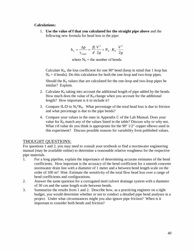
Calculations:
1. Use the value of f that you calculated for the straight pipe above and the
following new formula for head loss in the pipe:
g
VKN
g
V
d
fLbb
22γ
Δph
22
water
L
where Nb = the number of bends.
Calculate Kb, the loss coefficient for one 90º bend (keep in mind that 1 loop has
Nb = 4 bends). Do this calculation for both the one-loop and two-loop pipes.
Should the Kb values that are calculated for the one-loop and two-loop pipes be
similar? Explain.
2. Calculate Kb taking into account the additional length of pipe added by the bends.
How much does the value of Kb change when you account for the additional
length? How important is it to include it?
3. Compare fL/D to Nb*Kb. What percentage of the total head loss is due to friction
and what percentage is due to the pipe bends?
4. Compare your values to the ones in Appendix C of the Lab Manual. Does your
value for Kb match any of the values listed in the table? Discuss why or why not.
What r/d value do you think is appropriate for the 90º 1/2" copper elbows used in
this experiment? Discuss possible reasons for variability from published values.
THOUGHT QUESTIONS: For questions 1 and 2, you may need to consult your textbook or find a stormwater engineering
manual (may be available online) to determine a reasonable relative roughness for the respective
pipe materials.
1. For a long pipeline, explain the importance of determining accurate estimates of the bend
coefficients. How important is the accuracy of the bend coefficient for a smooth concrete
stormwater drain line with a diameter of 1 meter and a between bend length scale on the
order of 100 m? Hint: Estimate the sensitivity of the total flow head loss over a range of
bend coefficients and configurations.
2. Answer the same question for a corrugated steel culvert drainage system with a diameter
of 30 cm and the same length scale between bends.
3. Summarize the results from 1 and 2. Describe how, as a practicing engineer on a tight
budget, you would determine whether or not to conduct a detailed pipe bend analyses in a
project. Under what circumstances might you also ignore pipe friction? When is it
important to consider both bends and friction?
41
CE 3502 FLUID MECHANICS
Laboratory Experiment #8
PIPE NETWORKS
This exercise requires the solution of three exercises involving pipe network problems (e.g.,
Crowe et al., Chapter 10.10). The solver tool from Excel will be used to solve the systems of
equations that arise. The same techniques can be applied to more complicated systems
encountered in engineering applications.
You may find that there are multiple possible formulations to solve a single problem. A
consistent sign convention is essential. The example provided in EXERCISE 1 uses the
following sign conventions.
Loop: Head loss in the direction of flow is positive (+)
Head gain in the direction of flow is negative (-)
Head loss in the opposite direction of flow is negative (-)
Node: Flow into the node is positive (+)
Flow out of the node is negative (-)
It is also important to select the right number of appropriate equations (i.e. one equation for each
unknown, no more, no less).
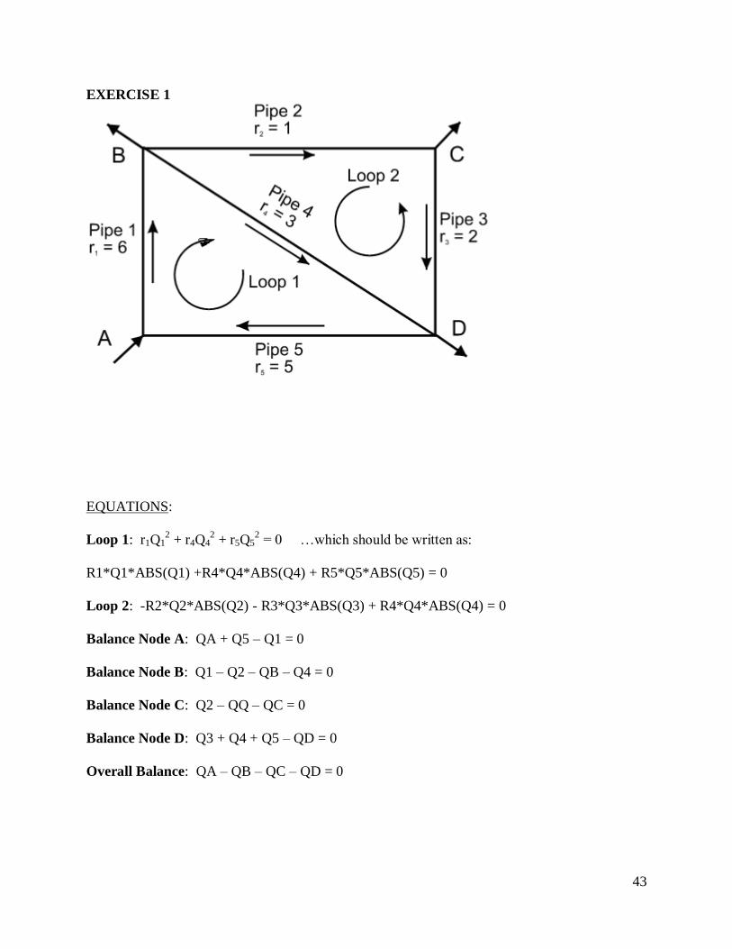
EXERCISE 1
The solution to this pipe network has been prepared in advance. Be sure to check the equations
for each balance and for each loop. (Hint: There is an error in one of the equations)
Case 1: B = 20, C = 50, D = 30 Case 2: B = 0, C = 0, D = 100
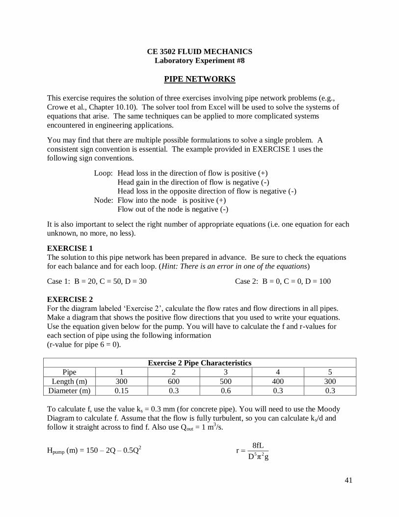
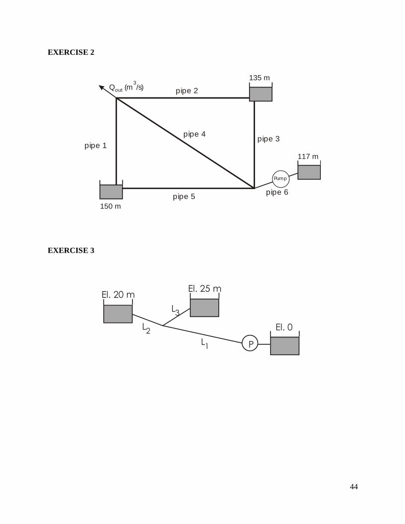
EXERCISE 2
For the diagram labeled ‘Exercise 2’, calculate the flow rates and flow directions in all pipes.
Make a diagram that shows the positive flow directions that you used to write your equations.
Use the equation given below for the pump. You will have to calculate the f and r-values for
each section of pipe using the following information
(r-value for pipe 6 = 0).
Exercise 2 Pipe Characteristics
Pipe 1 2 3 4 5
Length (m) 300 600 500 400 300
Diameter (m) 0.15 0.3 0.6 0.3 0.3
To calculate f, use the value ks = 0.3 mm (for concrete pipe). You will need to use the Moody
Diagram to calculate f. Assume that the flow is fully turbulent, so you can calculate ks/d and
follow it straight across to find f. Also use Qout = 1 m3/s.
Hpump (m) = 150 – 2Q – 0.5Q2
gπD
8fLr
25
42
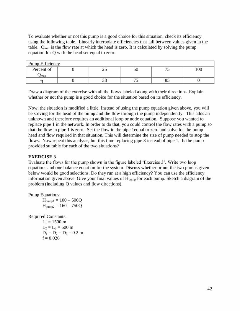
To evaluate whether or not this pump is a good choice for this situation, check its efficiency
using the following table. Linearly interpolate efficiencies that fall between values given in the
table. Qmax is the flow rate at which the head is zero. It is calculated by solving the pump
equation for Q with the head set equal to zero.
Pump Efficiency
Percent of
Qmax
0 25 50 75 100
0 38 75 85 0
Draw a diagram of the exercise with all the flows labeled along with their directions. Explain
whether or not the pump is a good choice for the situation based on its efficiency.
Now, the situation is modified a little. Instead of using the pump equation given above, you will
be solving for the head of the pump and the flow through the pump independently. This adds an
unknown and therefore requires an additional loop or node equation. Suppose you wanted to
replace pipe 1 in the network. In order to do that, you could control the flow rates with a pump so
that the flow in pipe 1 is zero. Set the flow in the pipe 1equal to zero and solve for the pump
head and flow required in that situation. This will determine the size of pump needed to stop the
flows. Now repeat this analysis, but this time replacing pipe 3 instead of pipe 1. Is the pump
provided suitable for each of the two situations?
EXERCISE 3
Evaluate the flows for the pump shown in the figure labeled ‘Exercise 3’. Write two loop
equations and one balance equation for the system. Discuss whether or not the two pumps given
below would be good selections. Do they run at a high efficiency? You can use the efficiency
information given above. Give your final values of Hpump for each pump. Sketch a diagram of the
problem (including Q values and flow directions).
Pump Equations:
Hpump1 = 100 – 500Q
Hpump2 = 160 – 750Q
Required Constants:
L1 = 1500 m
L2 = L3 = 600 m
D1 = D2 = D3 = 0.2 m
f = 0.026
43
EXERCISE 1
EQUATIONS:
Loop 1: r1Q12 + r4Q4
2 + r5Q5
2 = 0 …which should be written as:
R1*Q1*ABS(Q1) +R4*Q4*ABS(Q4) + R5*Q5*ABS(Q5) = 0
Loop 2: -R2*Q2*ABS(Q2) - R3*Q3*ABS(Q3) + R4*Q4*ABS(Q4) = 0
Balance Node A: QA + Q5 – Q1 = 0
Balance Node B: Q1 – Q2 – QB – Q4 = 0
Balance Node C: Q2 – QQ – QC = 0
Balance Node D: Q3 + Q4 + Q5 – QD = 0
Overall Balance: QA – QB – QC – QD = 0
44
EXERCISE 2
Q (m /s)out
3
Pump
135 m
117 m
150 m
pipe 1
pipe 4
pipe 5
pipe 3
pipe 2
pipe 6
EXERCISE 3
El. 20 m El. 25 m
El. 0
P L 1
L 2
L 3
45
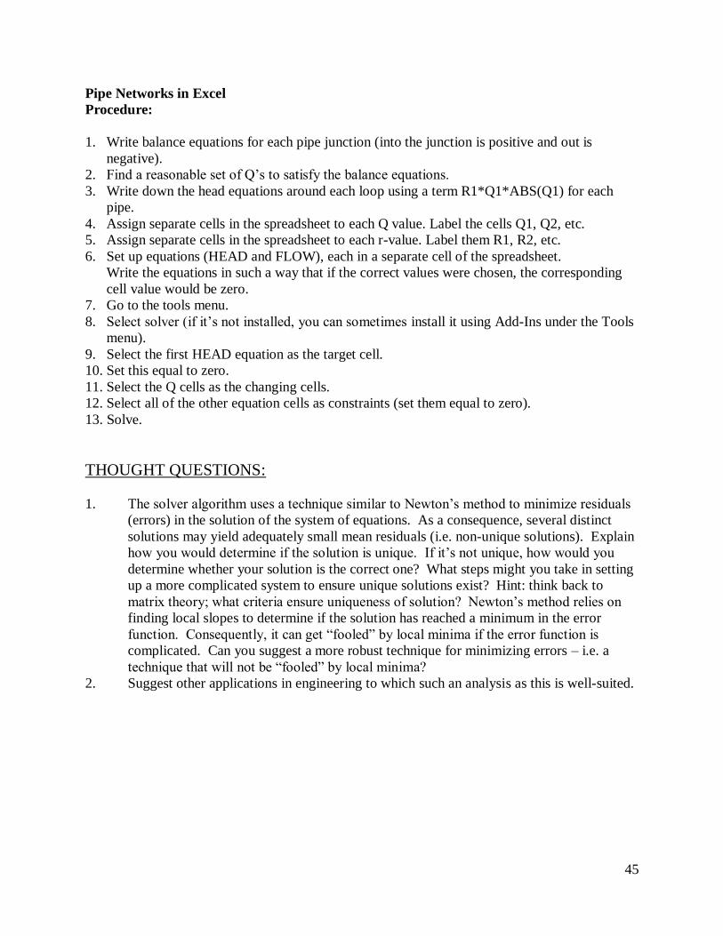
Pipe Networks in Excel
Procedure:
1. Write balance equations for each pipe junction (into the junction is positive and out is
negative).
2. Find a reasonable set of Q’s to satisfy the balance equations.
3. Write down the head equations around each loop using a term R1*Q1*ABS(Q1) for each
pipe.
4. Assign separate cells in the spreadsheet to each Q value. Label the cells Q1, Q2, etc.
5. Assign separate cells in the spreadsheet to each r-value. Label them R1, R2, etc.
6. Set up equations (HEAD and FLOW), each in a separate cell of the spreadsheet.
Write the equations in such a way that if the correct values were chosen, the corresponding
cell value would be zero.
7. Go to the tools menu.
8. Select solver (if it’s not installed, you can sometimes install it using Add-Ins under the Tools
menu).
9. Select the first HEAD equation as the target cell.
10. Set this equal to zero.
11. Select the Q cells as the changing cells.
12. Select all of the other equation cells as constraints (set them equal to zero).
13. Solve.
THOUGHT QUESTIONS:
1. The solver algorithm uses a technique similar to Newton’s method to minimize residuals
(errors) in the solution of the system of equations. As a consequence, several distinct
solutions may yield adequately small mean residuals (i.e. non-unique solutions). Explain
how you would determine if the solution is unique. If it’s not unique, how would you
determine whether your solution is the correct one? What steps might you take in setting
up a more complicated system to ensure unique solutions exist? Hint: think back to
matrix theory; what criteria ensure uniqueness of solution? Newton’s method relies on
finding local slopes to determine if the solution has reached a minimum in the error
function. Consequently, it can get “fooled” by local minima if the error function is
complicated. Can you suggest a more robust technique for minimizing errors – i.e. a
technique that will not be “fooled” by local minima?
2. Suggest other applications in engineering to which such an analysis as this is well-suited.
46
CE 3502 FLUID MECHANICS
Laboratory Experiment #9
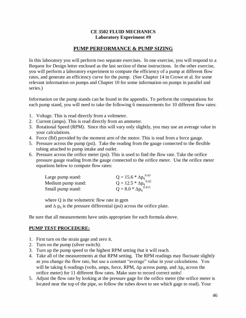
PUMP PERFORMANCE & PUMP SIZING
In this laboratory you will perform two separate exercises. In one exercise, you will respond to a
Request for Design letter enclosed as the last section of these instructions. In the other exercise,
you will perform a laboratory experiment to compute the efficiency of a pump at different flow
rates, and generate an efficiency curve for the pump. (See Chapter 14 in Crowe et al. for some
relevant information on pumps and Chapter 10 for some information on pumps in parallel and
series.)
Information on the pump stands can be found in the appendix. To perform the computations for
each pump stand, you will need to take the following 6 measurements for 10 different flow rates:
1. Voltage. This is read directly from a voltmeter.
2. Current (amps). This is read directly from an ammeter.
3. Rotational Speed (RPM). Since this will vary only slightly, you may use an average value in
your calculations.
4. Force (lbf) provided by the moment arm of the motor. This is read from a force gauge.
5. Pressure across the pump (psi). Take the reading from the gauge connected to the flexible
tubing attached to pump intake and outlet.
6. Pressure across the orifice meter (psi). This is used to find the flow rate. Take the orifice
pressure gauge reading from the gauge connected to the orifice meter. Use the orifice meter
equations below to compute flow rates:
Large pump stand: Q = 15.6 * pq0.43
Medium pump stand: Q = 12.5 * pq 0.42
Small pump stand: Q = 8.0 * pq 0.415
where Q is the volumetric flow rate in gpm
and pq is the pressure differential (psi) across the orifice plate.
Be sure that all measurements have units appropriate for each formula above.
PUMP TEST PROCEDURE:
1. First turn on the strain gage and zero it.
2. Turn on the pump (silver switch).
3. Turn up the pump speed to the highest RPM setting that it will reach.
4. Take all of the measurements at that RPM setting. The RPM readings may fluctuate slightly
as you change the flow rate, but use a constant “average” value in your calculations. You
will be taking 6 readings (volts, amps, force, RPM, p across pump, and pq across the
orifice meter) for 11 different flow rates. Make sure to record correct units!
5. Adjust the flow rate by looking at the pressure gage for the orifice meter (the orifice meter is
located near the top of the pipe, so follow the tubes down to see which gage to read). Your
47
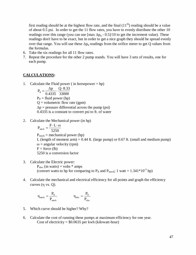
first reading should be at the highest flow rate, and the final (11th
) reading should be a value
of about 0.5 psi. In order to get the 11 flow rates, you have to evenly distribute the other 10
readings over this range (you can use [max pq - 0.5]/10 to get the increment value). These
readings don't have to be exact, but in order to get a nice graph they should be spread evenly
over that range. You will use these pq readings from the orifice meter to get Q values from
the formulas.
6. Take the six readings for all 11 flow rates.
7. Repeat the procedure for the other 2 pump stands. You will have 3 sets of results, one for
each pump.
CALCULATIONS:
1. Calculate the Fluid power ( in horsepower = hp)
33000
8.33Q
0.4335
Δp Pfl
Pfl = fluid power (hp)
Q = volumetric flow rate (gpm)
p = pressure differential across the pump (psi)
0.4335 is a constant to convert psi to ft. of water
2. Calculate the Mechanical power (in hp)
5250
ωLFPmech
Pmech = mechanical power (hp)
L (length of moment arm) = 0.44 ft. (large pump) or 0.67 ft. (small and medium pump)
= angular velocity (rpm)
F = force (lb)
5250 is a conversion factor
3. Calculate the Electric power:
Pelec (in watts) = volts * amps
(convert watts to hp for comparing to Pfl and Pmech; 1 watt = 1.341*10-3
hp)
4. Calculate the mechanical and electrical efficiency for all points and graph the efficiency
curves ( vs. Q).
elec
flelec
mech
flmech
P
P η
P
Pη
5. Which curve should be higher? Why?
6. Calculate the cost of running these pumps at maximum efficiency for one year.
Cost of electricity = $0.0635 per kwh (kilowatt-hour)
48
Northern Construction Company
18 Duck Street
Wild Goose, Minnesota 56708
April xx, 20xx
Handi Mann, Design Engineer
Water Resource Specialists
130 Main Street
Minneapolis, MN 55414
Dear Dr. Mann,
We have an opportunity to purchase two pumps at a very reasonable price from a new company.
This firm utilizes a universal design to manufacture pumps with different capacities. The pump
sizes include 11.0", 10.2 ", 9.6" and 8.1" diameter pumps. All four pumps operate at 1750 rpm.
In the near future, we will be working on two different excavation projects that have significantly
different pumping requirements. These are:
1. 200’ of head at 3600 gpm
2. 80’ of head at 16500 gpm
Please select a maximum of two pumps that will satisfy both of these requirements, since we
wish to use them on both projects. The non-dimensional pump data, as supplied by the
manufacturer, are enclosed.
Please call me at 218-623-3245 or E-mail me at [email protected] if you require any further
information.
Very truly yours
Ican Shovel
President
49
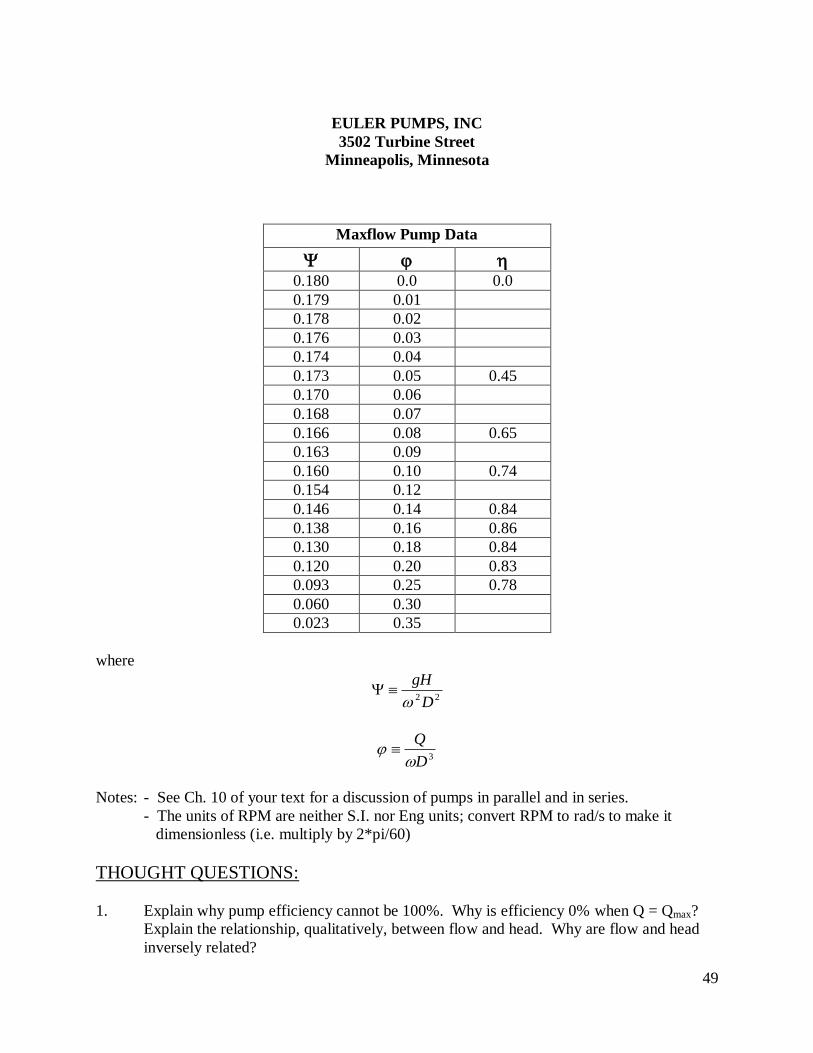
EULER PUMPS, INC
3502 Turbine Street
Minneapolis, Minnesota
Maxflow Pump Data
0.180 0.0 0.0
0.179 0.01
0.178 0.02
0.176 0.03
0.174 0.04
0.173 0.05 0.45
0.170 0.06
0.168 0.07
0.166 0.08 0.65
0.163 0.09
0.160 0.10 0.74
0.154 0.12
0.146 0.14 0.84
0.138 0.16 0.86
0.130 0.18 0.84
0.120 0.20 0.83
0.093 0.25 0.78
0.060 0.30
0.023 0.35
where
22 D
gH
3D
Q
Notes: - See Ch. 10 of your text for a discussion of pumps in parallel and in series.
- The units of RPM are neither S.I. nor Eng units; convert RPM to rad/s to make it
dimensionless (i.e. multiply by 2*pi/60)
THOUGHT QUESTIONS:
1. Explain why pump efficiency cannot be 100%. Why is efficiency 0% when Q = Qmax?
Explain the relationship, qualitatively, between flow and head. Why are flow and head
inversely related?
50
Appendix A: Useful Equations
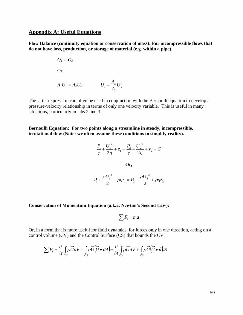
Flow Balance (continuity equation or conservation of mass): For incompressible flows that
do not have loss, production, or storage of material (e.g. within a pipe).
Q1 = Q2
Or,
A1U1 = A2U2 2
1
21 U
A
AU
The latter expression can often be used in conjunction with the Bernoulli equation to develop a
pressure-velocity relationship in terms of only one velocity variable. This is useful in many
situations, particularly in labs 2 and 3.
Bernoulli Equation: For two points along a streamline in steady, incompressible,
irrotational flow (Note: we often assume these conditions to simplify reality).
Czg
UPz
g
UP 2
2
221
2
11
22
Or,
2
2
221
2
11
22gz
UPgz
UP
Conservation of Momentum Equation (a.k.a. Newton’s Second Law):
maFi
Or, in a form that is more useful for fluid dynamics, for forces only in one direction, acting on a
control volume (CV) and the Control Surface (CS) that bounds the CV,
dSnUUdVUt
dAUUdVUt
FCSCVCSCV
i
ˆ
51
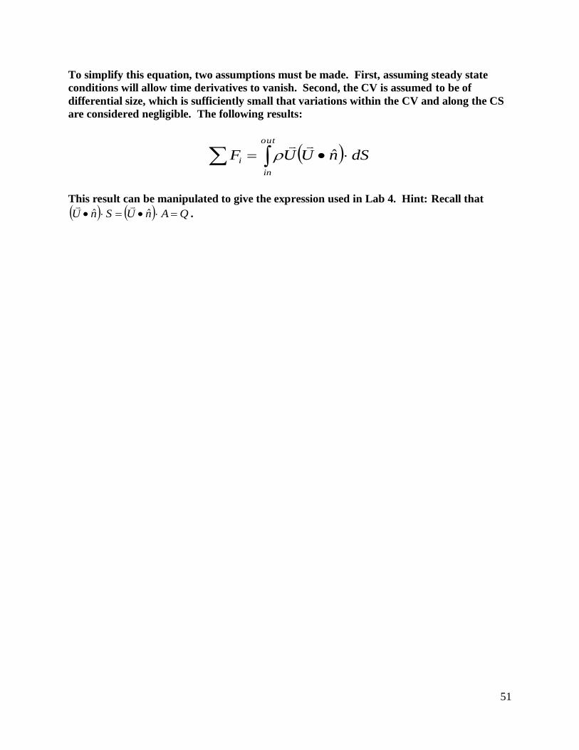
To simplify this equation, two assumptions must be made. First, assuming steady state
conditions will allow time derivatives to vanish. Second, the CV is assumed to be of
differential size, which is sufficiently small that variations within the CV and along the CS
are considered negligible. The following results:
dSnUUF
out
in
i ˆ
This result can be manipulated to give the expression used in Lab 4. Hint: Recall that
QAnUSnU ˆˆ
.
52
Appendix B: Useful techniques for working with lab data.
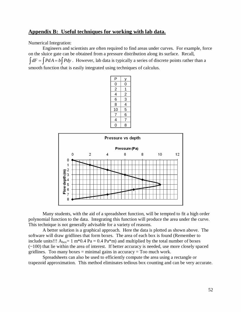
Numerical Integration:
Engineers and scientists are often required to find areas under curves. For example, force
on the sluice gate can be obtained from a pressure distribution along its surface. Recall,
PdybAPddF . However, lab data is typically a series of discrete points rather than a
smooth function that is easily integrated using techniques of calculus.
P y
0 0
2 1
4 2
6 3
8 4
10 5
7 6
4 7
0 8
Many students, with the aid of a spreadsheet function, will be tempted to fit a high order
polynomial function to the data. Integrating this function will produce the area under the curve.
This technique is not generally advisable for a variety of reasons.
A better solution is a graphical approach. Here the data is plotted as shown above. The
software will draw gridlines that form boxes. The area of each box is found (Remember to
include units!!! Abox= 1 m*0.4 Pa = 0.4 Pa*m) and multiplied by the total number of boxes
(~100) that lie within the area of interest. If better accuracy is needed, use more closely spaced
gridlines. Too many boxes = minimal gains in accuracy = Too much work.
Spreadsheets can also be used to efficiently compute the area using a rectangle or
trapezoid approximation. This method eliminates tedious box counting and can be very accurate.
53
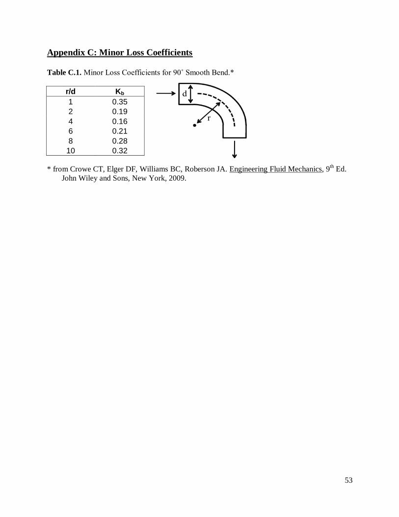
Appendix C: Minor Loss Coefficients
Table C.1. Minor Loss Coefficients for 90˚ Smooth Bend.*
r/d Kb
1 0.35
2 0.19
4 0.16
6 0.21
8 0.28
10 0.32
* from Crowe CT, Elger DF, Williams BC, Roberson JA. Engineering Fluid Mechanics, 9th Ed.
John Wiley and Sons, New York, 2009.
54
Appendix D: User’s Manual for Pump Testing Stand
Overview
The Pump Testing Stand was designed and constructed to demonstrate operational characteristics
of centrifugal pump systems. The Pump Testing Stand achieves these goals by allowing the
students to vary the motor RPM and pressure across the pump by adjusting a throttling valve to
change the loss coefficients of the piping system which the pump supplies with water. The Pump
Testing Stand has sensors showing the motor voltage, current, RPM, torque, pump pressure, and
flow in the system. Knowledge of these parameters allows the students to calculate electrical
power into the system, mechanical horsepower to the pump, and useful power supplied by the
pump. There are three different Pump Testing Stands with different impeller diameters allowing
the instructor to highlight the effects of changing impeller diameters upon the flow and pressure
characteristics of a pump.
Pump Testing Stands
Each of the stands has a 3/4 Horsepower (hp) variable speed DC electric motor. The motor has a
maximum rotational speed of 1750 revolutions per minute (RPM). The motor controllers allow
the rotational speed of the motor to be infinitely varied from 350 to 1750 RPM. Once set, the
rotational speed stays constant regardless of load. Motor manufacturer’s specifications are listed
separately.
The motors of each pump testing stand are directly coupled to a centrifugal pump. Each of the
three stands has a different diameter impeller on the centrifugal pump. The fluid flow rate is
measured by an orifice plate. Discharge from the pumps is controlled by gate valves.
Mechanical Power
The motor shaft is suspended by two ball bearings, leaving the housing of the motor free to
rotate. This allows the measurement of the reaction torque from the operation of the motor. This
is accomplished with a load cell to measure force, calibrated in pounds. The load cell is mounted
8” from the center of the motor shaft, with the load cell measuring force perpendicular to the
radius, as shown in Figure 1.
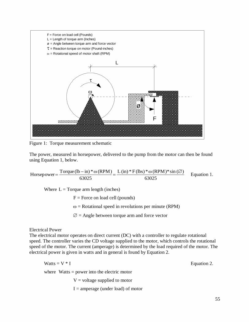
55
F = Force on load cell (Pounds)
L = Length of torque arm (Inches)
ø = Angle between torque arm and force vector
= Reaction torque on motor (Pound-inches)
= Rotational speed of motor shaft (RPM)
L
F
ø
Figure 1: Torque measurement schematic
The power, measured in horsepower, delivered to the pump from the motor can then be found
using Equation 1, below.
63025
)( sin * (RPM) ω * (lbs) F* (in) L
63025
(RPM) ω *in)(lb TorqueHorsepower
Equation 1.
Where L = Torque arm length (inches)
F = Force on load cell (pounds)
= Rotational speed in revolutions per minute (RPM)
= Angle between torque arm and force vector
Electrical Power
The electrical motor operates on direct current (DC) with a controller to regulate rotational
speed. The controller varies the CD voltage supplied to the motor, which controls the rotational
speed of the motor. The current (amperage) is determined by the load required of the motor. The
electrical power is given in watts and in general is found by Equation 2.
Watts = V * I Equation 2.
where Watts = power into the electric motor
V = voltage supplied to motor
I = amperage (under load) of motor
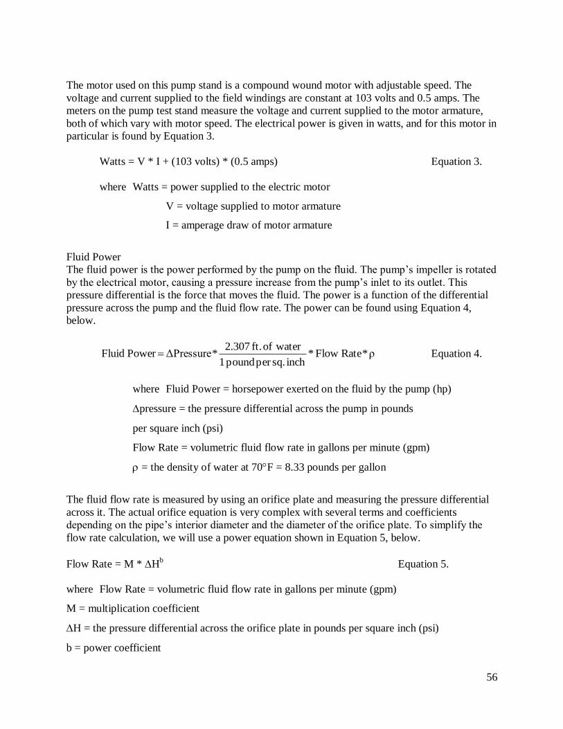
56
The motor used on this pump stand is a compound wound motor with adjustable speed. The
voltage and current supplied to the field windings are constant at 103 volts and 0.5 amps. The
meters on the pump test stand measure the voltage and current supplied to the motor armature,
both of which vary with motor speed. The electrical power is given in watts, and for this motor in
particular is found by Equation 3.
Watts = V * I + (103 volts) * (0.5 amps) Equation 3.
where Watts = power supplied to the electric motor
V = voltage supplied to motor armature
I = amperage draw of motor armature
Fluid Power
The fluid power is the power performed by the pump on the fluid. The pump’s impeller is rotated
by the electrical motor, causing a pressure increase from the pump’s inlet to its outlet. This
pressure differential is the force that moves the fluid. The power is a function of the differential
pressure across the pump and the fluid flow rate. The power can be found using Equation 4,
below.
ρ * Flow Rate* inch sq.per pound 1
waterof ft. 2.307 * ΔPressure Power Fluid Equation 4.
where Fluid Power = horsepower exerted on the fluid by the pump (hp)
pressure = the pressure differential across the pump in pounds
per square inch (psi)
Flow Rate = volumetric fluid flow rate in gallons per minute (gpm)
= the density of water at 70F = 8.33 pounds per gallon
The fluid flow rate is measured by using an orifice plate and measuring the pressure differential
across it. The actual orifice equation is very complex with several terms and coefficients
depending on the pipe’s interior diameter and the diameter of the orifice plate. To simplify the
flow rate calculation, we will use a power equation shown in Equation 5, below.
Flow Rate = M * Hb Equation 5.
where Flow Rate = volumetric fluid flow rate in gallons per minute (gpm)
M = multiplication coefficient
H = the pressure differential across the orifice plate in pounds per square inch (psi)
b = power coefficient
57
Efficiencies
In the above sections, power was calculated using units commonly used in practical applications.
For example, small electric motors are rated by their power in horsepower, now watts. Efficiency
is defined as the ratio of the useful energy output of a device to the energy input supplied to the
device. To calculate efficiencies, the energy units must be the same. For the previous
calculations, either watts or horsepower will suffice.
Power Conversion Factors:
1 Watt = 0.00134 Horsepower
1 Watt = 1 Joule per second
1 Horsepower = 745.7 Watts
1 Horsepower = 42.436 BTU per minute
Equation 6.
After converting the electrical, mechanical and fluid powers to the same units, the efficiencies
can be found.
suppliedinput Energy
outputenergy Useful y)(efficienc η Equation 7.
motor the tosuppliedenergy Electrical
fluid the topump by the suppliedenergy Fluidη
shaft pump the tosuppliedenergy Mechanical
fluid the topump by the suppliedenergy Fluidη
motor the tosuppliedenergy Electrical
shaft pump the tosuppliedenergy Mechanicalη
overall
pump
mechanical
Large Pump Testing Stand
This stand has a 3/4 Horsepower (hp) variable speed CD electric motor. The motor has a
maximum rotational speed of 1750 revolutions per minute (RPM). The pump is a centrifugal
type with an impeller diameter of 4.25” (inches). Manufacturer’s specifications are listed
separately.
The orifice pipe is a 1 1/4 PVC schedule 40 with an interior diameter of 1.38”. The orifice plate
is concentric, made of 1/8” brass sheeting with a 1/16”, 45 bevel on the downstream face. The
interior diameter of the orifice is 0.82”. The approximate flow rate is given by Equation 8.
Flow Rate = 15.6 * H0.43
Equation 8.
where Flow Rate = volumetric fluid flow rate in gallons per minute (gpm)
for the large test stand
H = the pressure differential across the orifice plate in pounds per square inch (psi)
58
Medium Pump Testing Stand
This stand has a 3/4 Horsepower (hp) variable speed DC electric motor. The motor has a
maximum rotational speed of 1750 revolutions per minute (RPM). The pump is a centrifugal
type with an impeller diameter of 3.75” (inches). Manufacturer’s specificat ions are listed
separately.
The orifice pipe is a 1 PVC schedule 40 with an interior diameter of 1.05”. The orifice plate is
concentric, made of 1/8” brass sheeting with an 1/16”, 45 bevel on the downstream face. The
interior diameter of the orifice is 0.70”. The approximate flow rate is given by Equation 9.
Flow Rate = 12.5 * H0.42
Equation 9.
where Flow Rate = volumetric fluid flow rate in gallons per minute (gpm)
for the medium pump test stand
H = the pressure differential across the orifice plate in pounds per square inch (psi)
Small Pump Testing Stand
The stand has a 3/4 horsepower (hp) variable speed DC electric motor. The motor has a
maximum rotational speed of 1750 revolutions per minute (RPM). The pump is a centrifugal
type with an impeller diameter of 3.56” (inches). Manufacturer’s specifications are listed
separately.
The orifice pipe is a 3/4 PVC schedule 40 with an interior diameter of 0.82”. The orifice plate is
concentric, made of 1/8” brass sheeting with a 1/16”, 45 bevel on the downstream face. The
interior diameter of the orifice is 0.55”. The approximate flow rate is given by Equation 10.
Flow Rate = 8.0 * H0.415
Equation 10.
where Flow Rate = volumetric fluid flow rate in gallons per minute (gpm)
for the small pump test stand
H = the pressure differential across the orifice plate in pounds per square inch (psi)

59
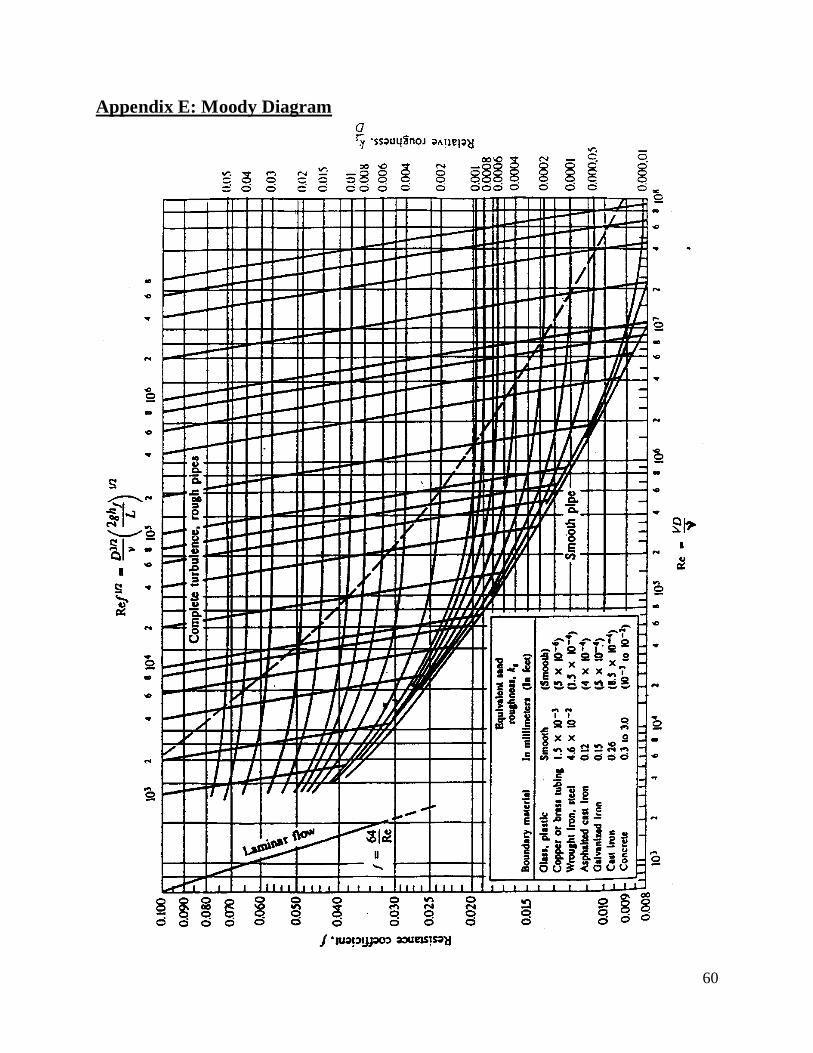
60
Appendix E: Moody Diagram