Ch06-Routing in WSNs

1Telecomm. Dept.Faculty of EEE

WSN‐2013HCMUT

Wireless Sensor Networks

Dr. –Ing. Vo Que SonEmail: [email protected]


WSN‐2013HCMUT

ContentChapter 5: MAC protocolsLow‐power linkIEEE 802.15.4 and Robust communicationPower on Link layerSchedule mechanism: TDMA, S‐MAC, Wise‐MAC,…Low‐Power listening: B‐MAC

Chapter 6: Routing in WSNsMulti‐hop communicationLink characteristicsTrickle algorithmProactive/reactive routing: AODV, DSR, CTP,…


WSN‐2013HCMUT

Wireless Ad‐hoc NetworksTwo types of wireless network: Infrastructured (WLAN)the mobile node can move while communicatingthe base stations are fixedas the node goes out of the range of a base station, it gets into the range of another base station

Infrastructureless or ad‐hocthe mobile node can move while communicatingthere are no fixed base stationsall the nodes in the network need to act as routers

In Latin “ad‐hoc” literally means “for this purpose only”. Then an ad‐hoc network can be regarded as “spontaneous network”


WSN‐2013HCMUT

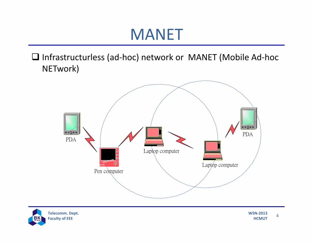
MANET Infrastructurless (ad‐hoc) network or MANET (Mobile Ad‐hoc

NETwork)

PDA

Pen computer

Laptop computer

Laptop computer

PDA


WSN‐2013HCMUT

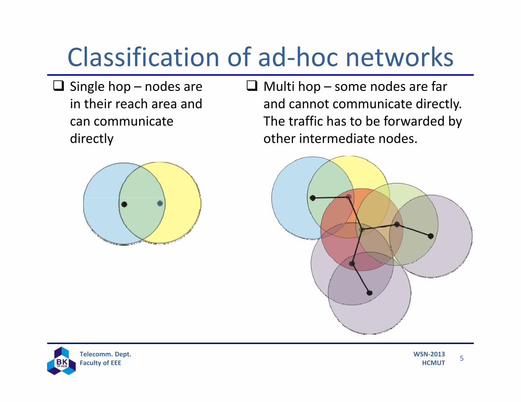
Classification of ad‐hoc networks Single hop – nodes are

in their reach area and can communicate directly

Multi hop – some nodes are far and cannot communicate directly. The traffic has to be forwarded by other intermediate nodes.


WSN‐2013HCMUT

Characteristics of an ad‐hoc networkCollection of mobile nodes forming a temporary networkNetwork topology changes frequently and unpredictablyNo centralized administration or standard support

services Each host is an independent routerHosts use wireless RF transceivers as network interface Number of nodes 10 to 100 or at most 1000Nodes/host are powerful and focus on how to keep the

mobile connection; high computation and high power consumption may be acceptable


WSN‐2013HCMUT

Classical View of Routing Connectivity between nodes defines the network graph.

Topology formation A Routing algorithm determines the sub‐graph that is used for

communication between nodes. Route formation, path selection

Packets are forwarded from source to destination over the routing subgraph At each node in the path, determine the recipient of the next hop

The selection at each hop is made based on the information at hand Sender address, current address, destination address, information in

the packet, information on the node. Table‐driven, source based, algorithmic, …Who knows the route? Do you determine it as you go?


WSN‐2013HCMUT

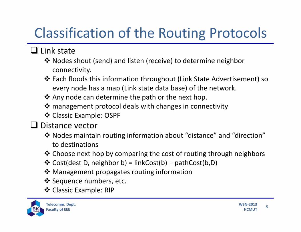
Classification of the Routing Protocols Link state

Nodes shout (send) and listen (receive) to determine neighbor connectivity.

Each floods this information throughout (Link State Advertisement) so every node has a map (Link state data base) of the network.

Any node can determine the path or the next hop.management protocol deals with changes in connectivity Classic Example: OSPF

Distance vector Nodes maintain routing information about “distance” and “direction”

to destinations Choose next hop by comparing the cost of routing through neighbors Cost(dest D, neighbor b) = linkCost(b) + pathCost(b,D)Management propagates routing information Sequence numbers, etc. Classic Example: RIP


WSN‐2013HCMUT

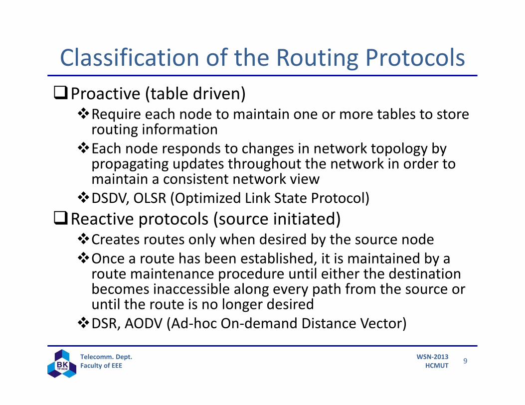
Classification of the Routing ProtocolsProactive (table driven)Require each node to maintain one or more tables to store routing information

Each node responds to changes in network topology by propagating updates throughout the network in order to maintain a consistent network view

DSDV, OLSR (Optimized Link State Protocol)Reactive protocols (source initiated)Creates routes only when desired by the source nodeOnce a route has been established, it is maintained by a route maintenance procedure until either the destination becomes inaccessible along every path from the source or until the route is no longer desired

DSR, AODV (Ad‐hoc On‐demand Distance Vector)


WSN‐2013HCMUT

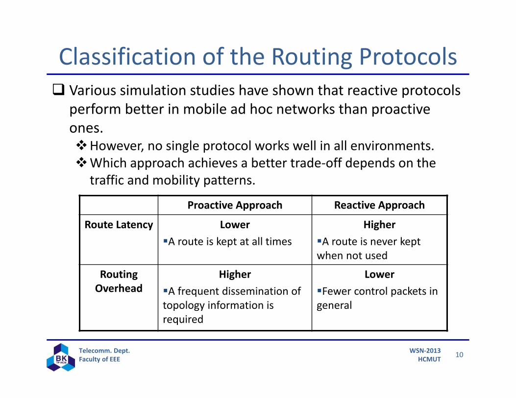
Classification of the Routing Protocols Various simulation studies have shown that reactive protocols

perform better in mobile ad hoc networks than proactive ones.However, no single protocol works well in all environments.Which approach achieves a better trade‐off depends on the

traffic and mobility patterns.

Proactive Approach Reactive Approach

Route Latency LowerA route is kept at all times

HigherA route is never kept when not used

Routing Overhead

HigherA frequent dissemination of topology information is required

LowerFewer control packets in general


WSN‐2013HCMUT

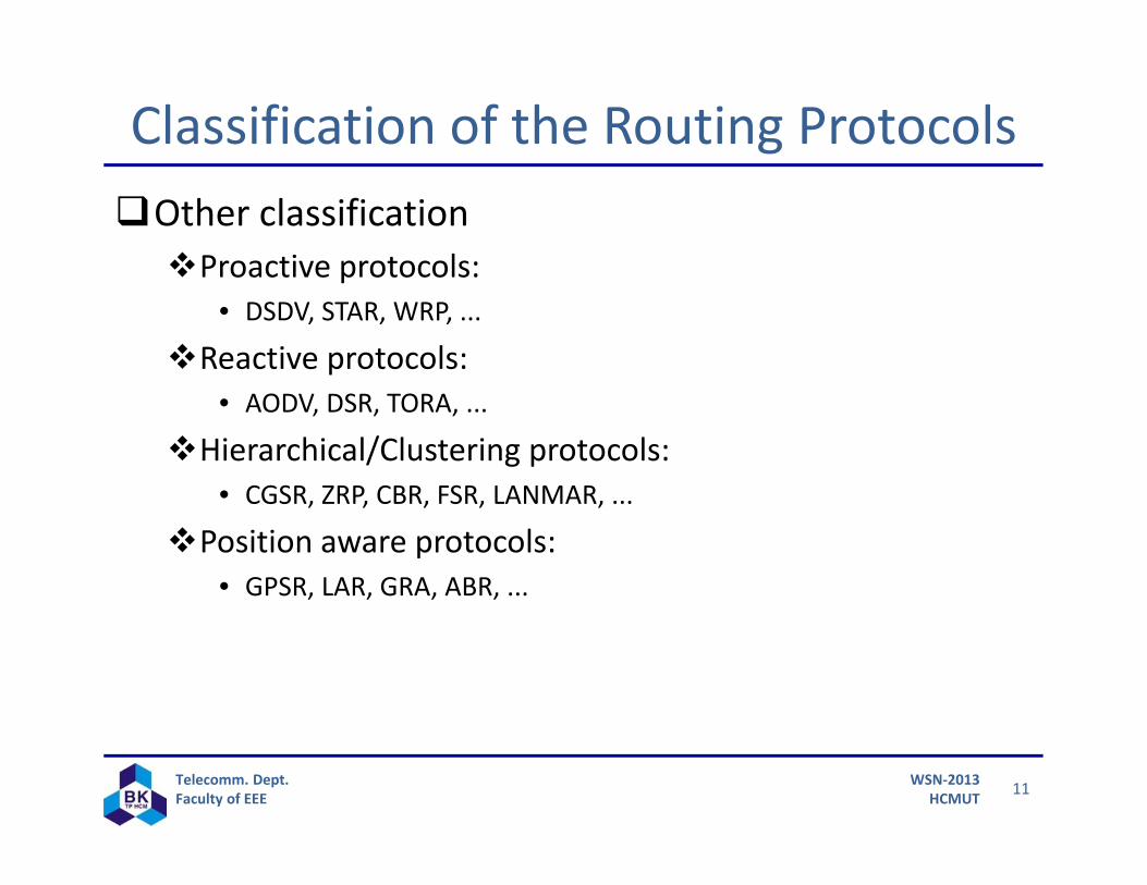
Classification of the Routing ProtocolsOther classificationProactive protocols:

• DSDV, STAR, WRP, ...

Reactive protocols: • AODV, DSR, TORA, ...

Hierarchical/Clustering protocols: • CGSR, ZRP, CBR, FSR, LANMAR, ...

Position aware protocols: • GPSR, LAR, GRA, ABR, ...


WSN‐2013HCMUT

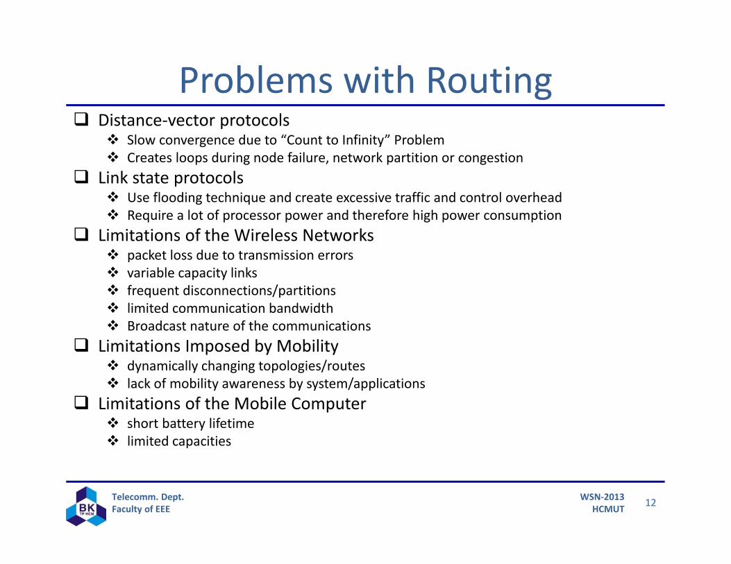
Problems with Routing Distance‐vector protocols

Slow convergence due to “Count to Infinity” Problem Creates loops during node failure, network partition or congestion

Link state protocols Use flooding technique and create excessive traffic and control overhead Require a lot of processor power and therefore high power consumption

Limitations of the Wireless Networks packet loss due to transmission errors variable capacity links frequent disconnections/partitions limited communication bandwidth Broadcast nature of the communications

Limitations Imposed by Mobility dynamically changing topologies/routes lack of mobility awareness by system/applications

Limitations of the Mobile Computer short battery lifetime limited capacities


WSN‐2013HCMUT

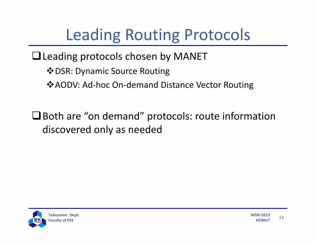
Leading Routing ProtocolsLeading protocols chosen by MANET DSR: Dynamic Source RoutingAODV: Ad‐hoc On‐demand Distance Vector Routing

Both are “on demand” protocols: route information discovered only as needed


WSN‐2013HCMUT

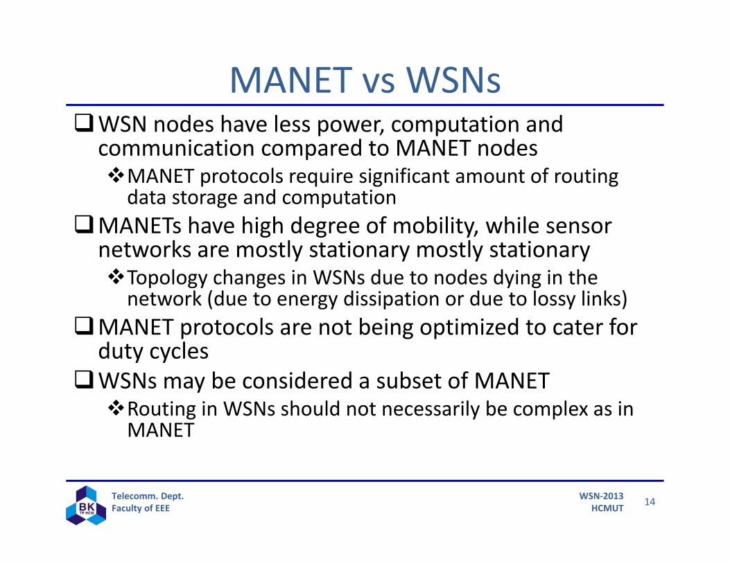
MANET vs WSNsWSN nodes have less power, computation and communication compared to MANET nodesMANET protocols require significant amount of routing data storage and computation

MANETs have high degree of mobility, while sensor networks are mostly stationary mostly stationaryTopology changes in WSNs due to nodes dying in the network (due to energy dissipation or due to lossy links)

MANET protocols are not being optimized to cater for duty cycles

WSNs may be considered a subset of MANETRouting in WSNs should not necessarily be complex as in MANET


WSN‐2013HCMUT

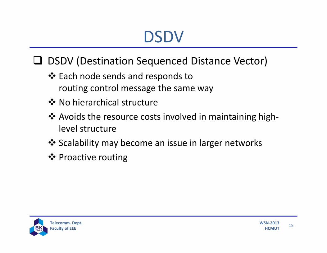
DSDV (Destination Sequenced Distance Vector) Each node sends and responds to

routing control message the same way No hierarchical structure Avoids the resource costs involved in maintaining high‐

level structure Scalability may become an issue in larger networks Proactive routing

DSDV


WSN‐2013HCMUT

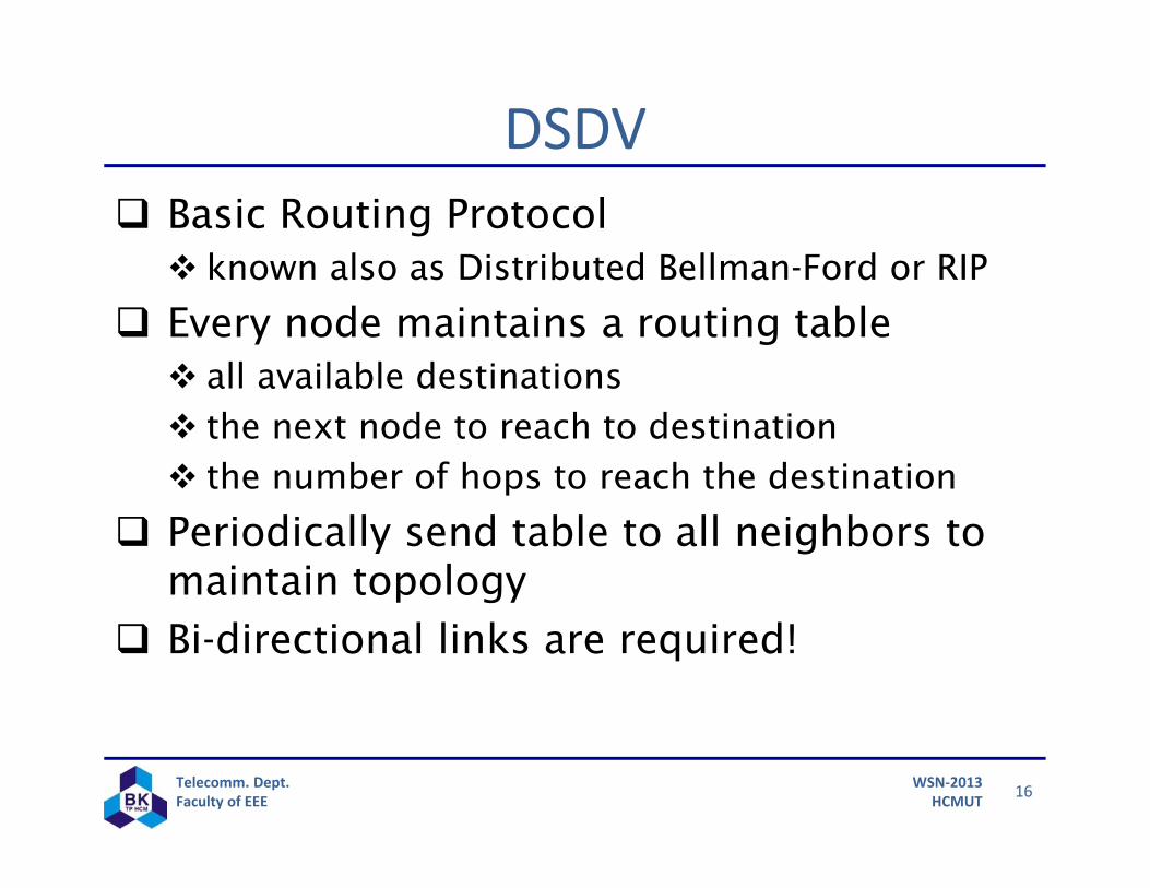
Basic Routing Protocol known also as Distributed Bellman-Ford or RIP

Every node maintains a routing table all available destinations the next node to reach to destination the number of hops to reach the destination

Periodically send table to all neighbors to maintain topology

Bi-directional links are required!

DSDV


WSN‐2013HCMUT

DSDV

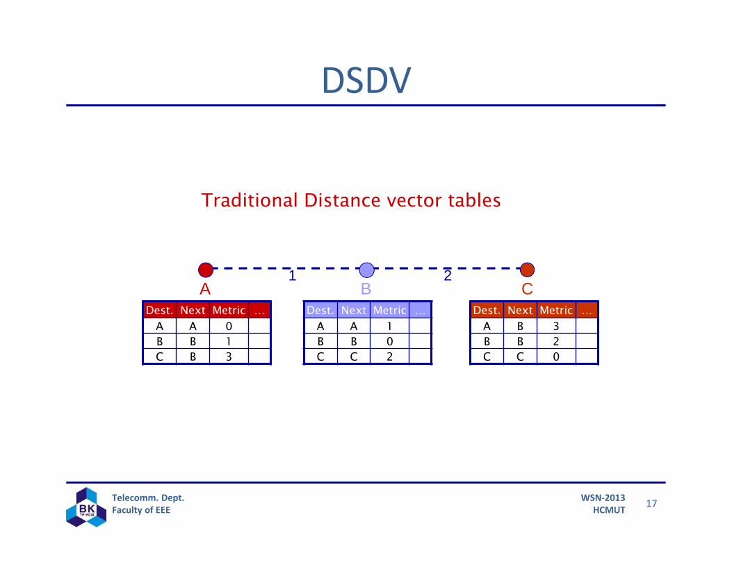
Traditional Distance vector tables

CDest. Next Metric …

A A 1B B 0C C 2

Dest. Next Metric …A A 0B B 1C B 3

1 2

Dest. Next Metric …A B 3B B 2C C 0

BA


WSN‐2013HCMUT

DSDV

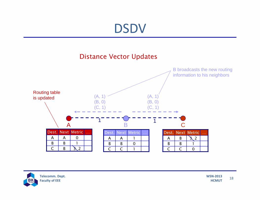
(A, 1)(B, 0)(C, 1)

(A, 1)(B, 0)(C, 1)

Distance Vector Updates

CDest. Next Metric …

A A 1B B 0C C 1

Dest. Next Metric …A A 0B B 1C B 3 2

1 1

Dest. Next Metric …A B 3 2B B 1C C 0

BA

B broadcasts the new routing information to his neighbors

Routing table is updated


WSN‐2013HCMUT

DSDV

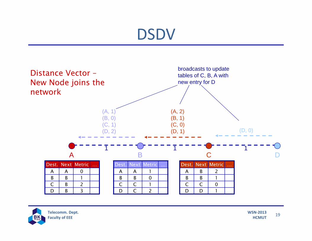
(D, 0)

(A, 2)(B, 1)(C, 0)(D, 1)

(A, 1)(B, 0)(C, 1)(D, 2)

Distance Vector –New Node joins the network

C1 1

BA D1

broadcasts to update tables of C, B, A with new entry for D

Dest. Next Metric …A B 2B B 1C C 0D D 1

Dest. Next Metric …A A 1B B 0C C 1D C 2

Dest. Next Metric …A A 0B B 1C B 2D B 3


WSN‐2013HCMUT

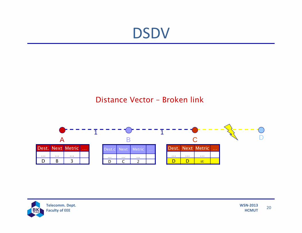
DSDV

Distance Vector – Broken link

C1 1

BA D1

Dest.c Next Metric …

… … …D C 2

Dest. Next Metric …… … …D B 3


Dest. Next Metric …… … …D D


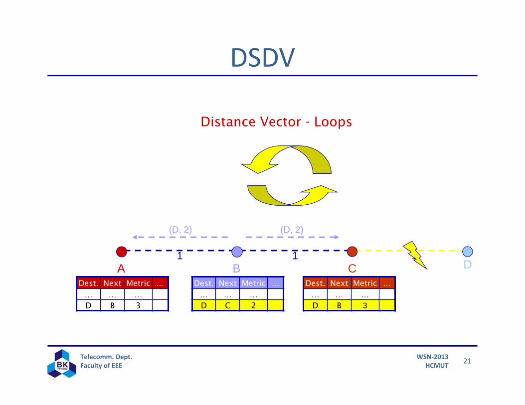
WSN‐2013HCMUT

DSDV

(D, 2)(D, 2)

Distance Vector - Loops

C1 1

BA D1


Dest. Next Metric …… … …D C 2



WSN‐2013HCMUT

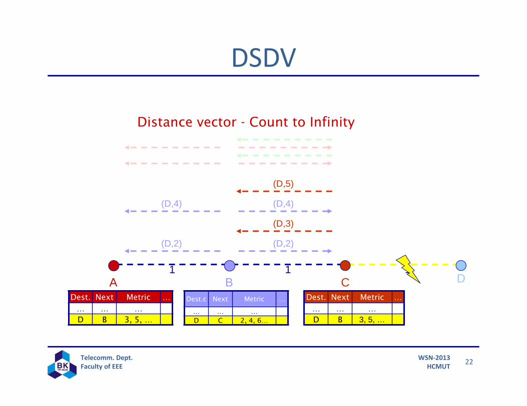
DSDV

(D,2)

(D,4)

(D,3)

(D,5)

(D,2)

(D,4)

Distance vector - Count to Infinity

C1 1

BA D1

Dest. Next Metric …… … …D B 3, 5, …

Dest. Next Metric …… … …D B 3, 5, …

Dest.c Next Metric …

… … …D C 2, 4, 6…


WSN‐2013HCMUT

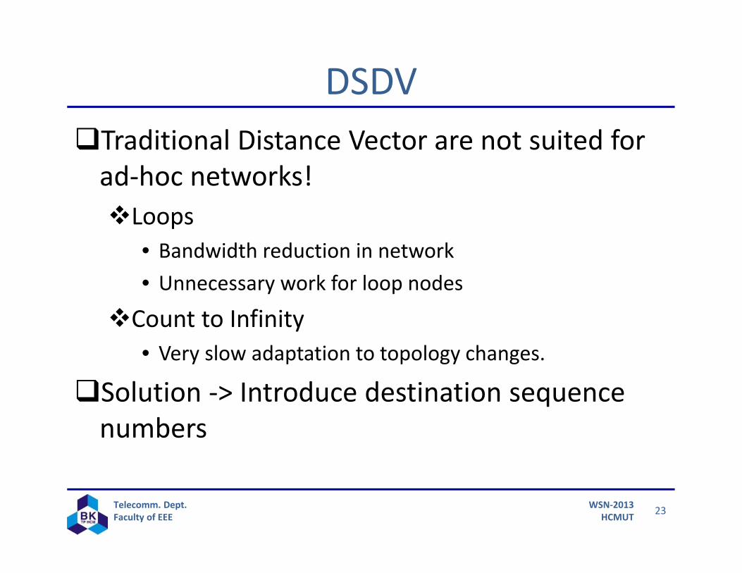
DSDVTraditional Distance Vector are not suited for ad‐hoc networks! Loops

• Bandwidth reduction in network• Unnecessary work for loop nodes

Count to Infinity• Very slow adaptation to topology changes.

Solution ‐> Introduce destination sequence numbers


WSN‐2013HCMUT

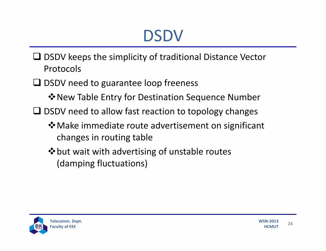
DSDV DSDV keeps the simplicity of traditional Distance Vector

Protocols DSDV need to guarantee loop freenessNew Table Entry for Destination Sequence Number

DSDV need to allow fast reaction to topology changesMake immediate route advertisement on significant changes in routing table

but wait with advertising of unstable routes(damping fluctuations)


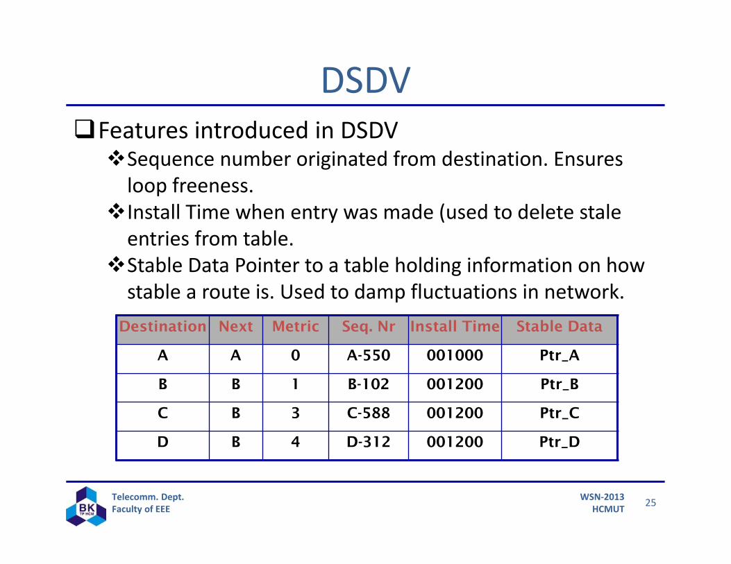
WSN‐2013HCMUT

DSDVFeatures introduced in DSDVSequence number originated from destination. Ensures loop freeness.

Install Time when entry was made (used to delete stale entries from table.

Stable Data Pointer to a table holding information on how stable a route is. Used to damp fluctuations in network.

Destination Next Metric Seq. Nr Install Time Stable Data

A A 0 A-550 001000 Ptr_A

B B 1 B-102 001200 Ptr_B

C B 3 C-588 001200 Ptr_C

D B 4 D-312 001200 Ptr_D


WSN‐2013HCMUT

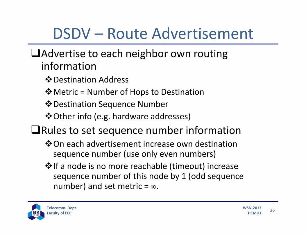
DSDV – Route AdvertisementAdvertise to each neighbor own routing informationDestination AddressMetric = Number of Hops to DestinationDestination Sequence NumberOther info (e.g. hardware addresses)

Rules to set sequence number informationOn each advertisement increase own destination sequence number (use only even numbers)

If a node is no more reachable (timeout) increase sequence number of this node by 1 (odd sequence number) and set metric = .


WSN‐2013HCMUT

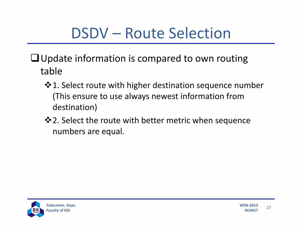
DSDV – Route SelectionUpdate information is compared to own routing table1. Select route with higher destination sequence number (This ensure to use always newest information from destination)

2. Select the route with better metric when sequence numbers are equal.


WSN‐2013HCMUT

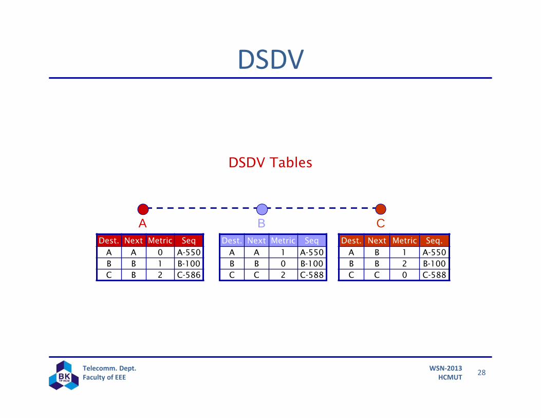
DSDV

DSDV Tables

CDest. Next Metric Seq

A A 1 A-550B B 0 B-100C C 2 C-588

Dest. Next Metric SeqA A 0 A-550B B 1 B-100C B 2 C-586

Dest. Next Metric Seq.A B 1 A-550B B 2 B-100C C 0 C-588

BA


WSN‐2013HCMUT

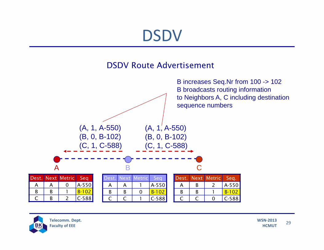
DSDV

(A, 1, A-550)(B, 0, B-102)(C, 1, C-588)

(A, 1, A-550)(B, 0, B-102)(C, 1, C-588)

DSDV Route Advertisement

CBA

B increases Seq.Nr from 100 -> 102B broadcasts routing information to Neighbors A, C including destination sequence numbers

Dest. Next Metric SeqA A 0 A-550B B 1 B-102C B 2 C-588

Dest. Next Metric SeqA A 1 A-550B B 0 B-102C C 1 C-588

Dest. Next Metric Seq.A B 2 A-550B B 1 B-102C C 0 C-588


WSN‐2013HCMUT

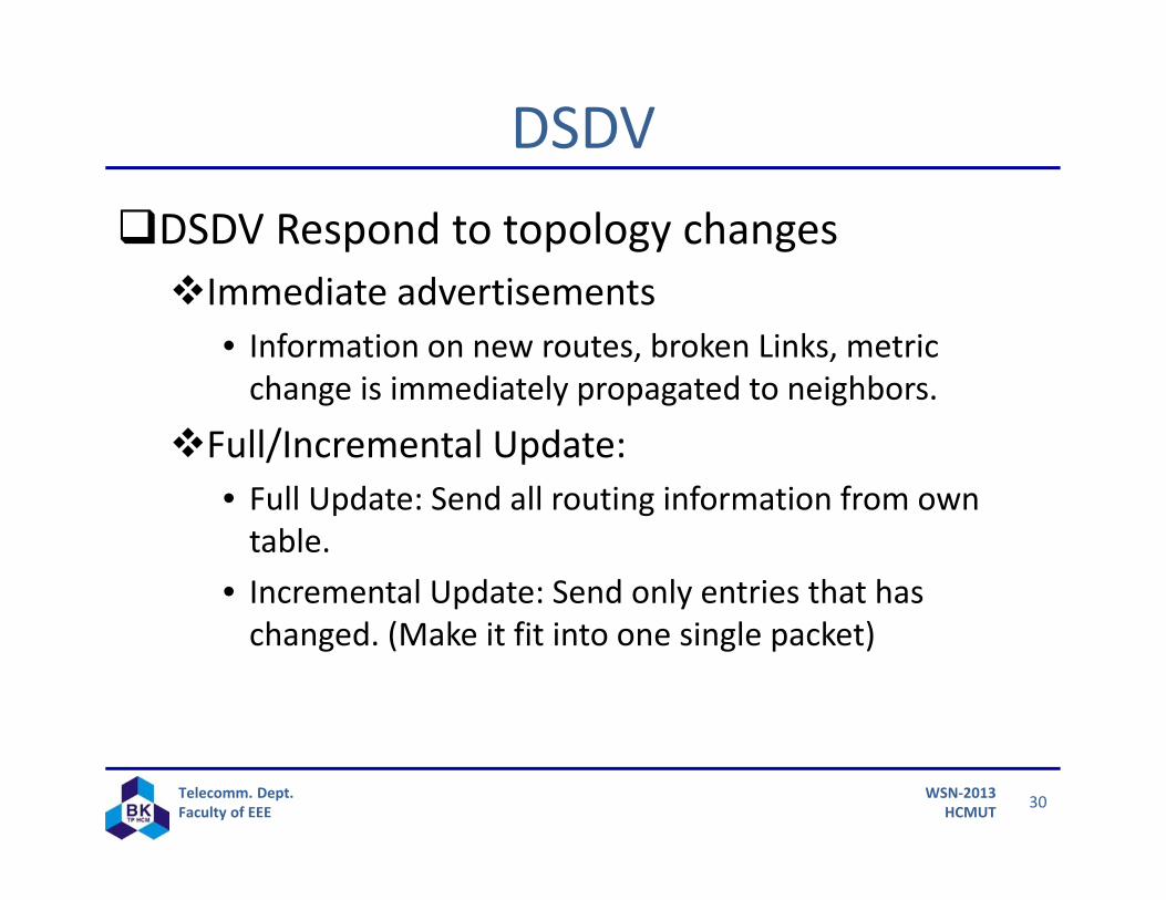
DSDVDSDV Respond to topology changesImmediate advertisements

• Information on new routes, broken Links, metric change is immediately propagated to neighbors.

Full/Incremental Update:• Full Update: Send all routing information from own table.

• Incremental Update: Send only entries that has changed. (Make it fit into one single packet)


WSN‐2013HCMUT

DSDV

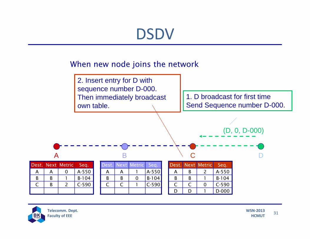
(D, 0, D-000)

When new node joins the network

CBA DDest. Next Metric Seq.

A A 0 A-550B B 1 B-104C B 2 C-590

Dest. Next Metric Seq.A A 1 A-550B B 0 B-104C C 1 C-590

Dest. Next Metric Seq.A B 2 A-550B B 1 B-104C C 0 C-590D D 1 D-000

1. D broadcast for first timeSend Sequence number D-000.

2. Insert entry for D with sequence number D-000.Then immediately broadcast own table.


WSN‐2013HCMUT

DSDV

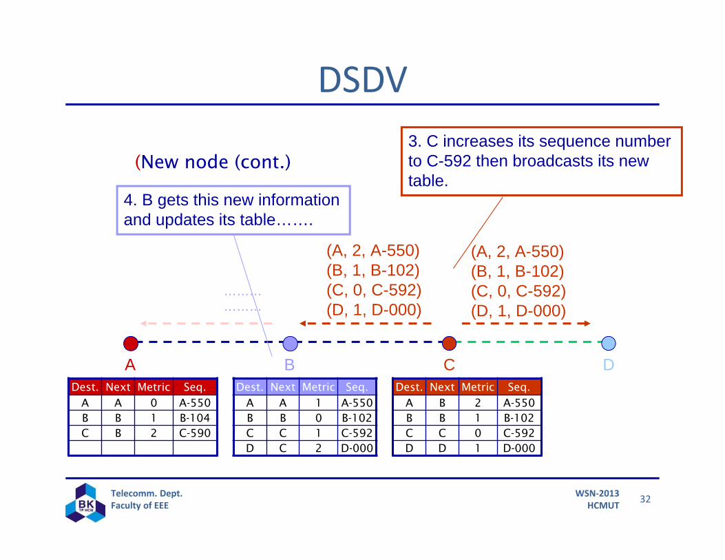
(A, 2, A-550)(B, 1, B-102)(C, 0, C-592)(D, 1, D-000)

(A, 2, A-550)(B, 1, B-102)(C, 0, C-592)(D, 1, D-000)

(New node (cont.)

CBA DDest. Next Metric Seq.

A A 1 A-550B B 0 B-102C C 1 C-592D C 2 D-000

Dest. Next Metric Seq.A A 0 A-550B B 1 B-104C B 2 C-590

Dest. Next Metric Seq.A B 2 A-550B B 1 B-102C C 0 C-592D D 1 D-000

………………

3. C increases its sequence number to C-592 then broadcasts its new table.

4. B gets this new information and updates its table…….


WSN‐2013HCMUT

DSDV

(D, 2, D-100)(D, 2, D-100)

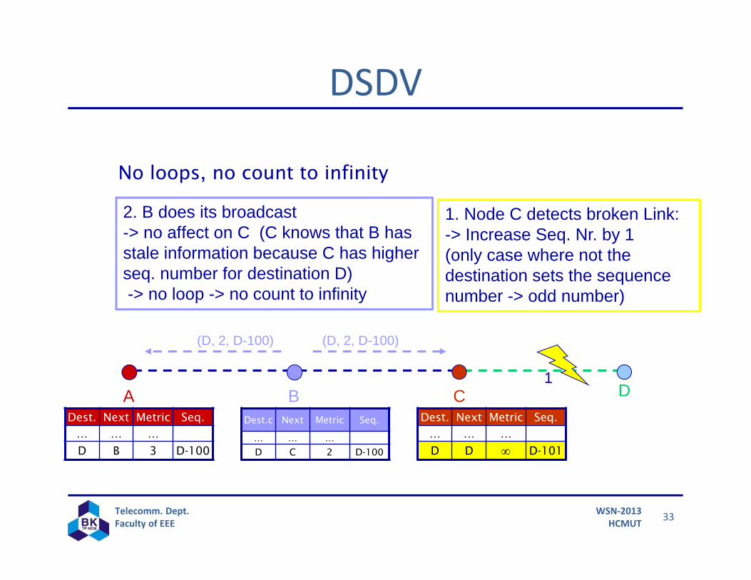
No loops, no count to infinity

CBA D1

Dest.c Next Metric Seq.

… … …

D C 2 D-100

Dest. Next Metric Seq.… … …

D B 3 D-100


D D D-101

1. Node C detects broken Link:-> Increase Seq. Nr. by 1(only case where not the destination sets the sequence number -> odd number)

2. B does its broadcast-> no affect on C (C knows that B has stale information because C has higher seq. number for destination D)-> no loop -> no count to infinity


WSN‐2013HCMUT

DSDV

(D, , D-101)(D, , D-101)

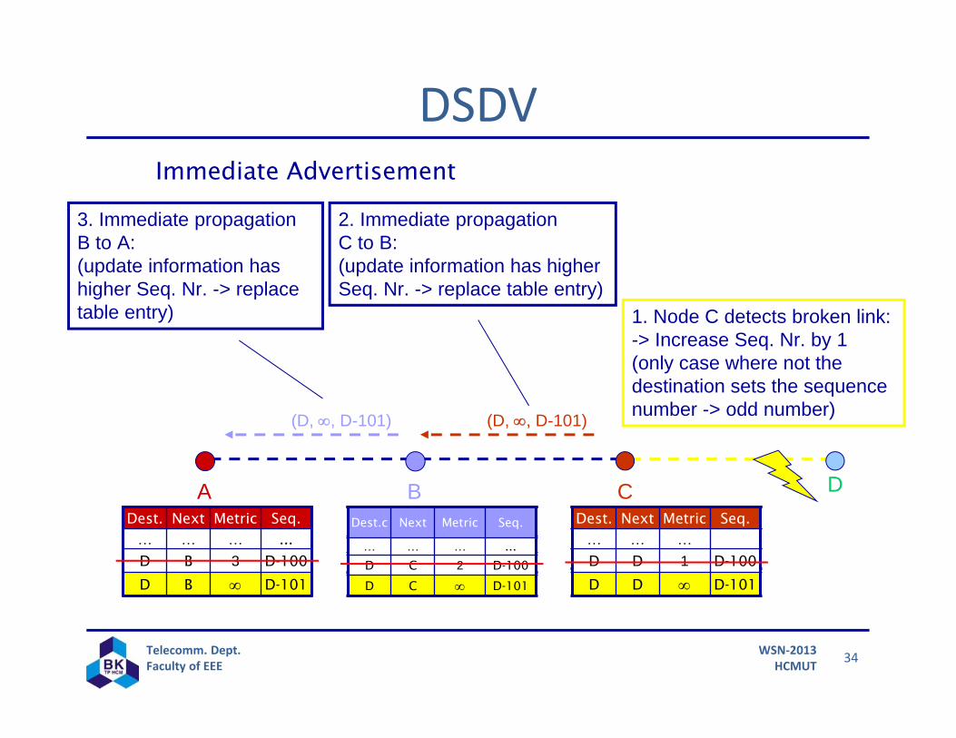
Immediate Advertisement

CBA DDest.c Next Metric Seq.

… … …

D C 3 D-100

Dest. Next Metric Seq.… … …D B 4 D-100

Dest. Next Metric Seq.… … …D B 1 D-100


D D 1 D-100

D D D-101

1. Node C detects broken link:-> Increase Seq. Nr. by 1(only case where not the destination sets the sequence number -> odd number)

3. Immediate propagation B to A:(update information has higher Seq. Nr. -> replace table entry)

2. Immediate propagationC to B:(update information has higher Seq. Nr. -> replace table entry)

Dest.c Next Metric Seq.

… … … ...

D C 2 D-100

D C D-101

Dest. Next Metric Seq.… … … ...

D B 3 D-100

D B D-101


WSN‐2013HCMUT

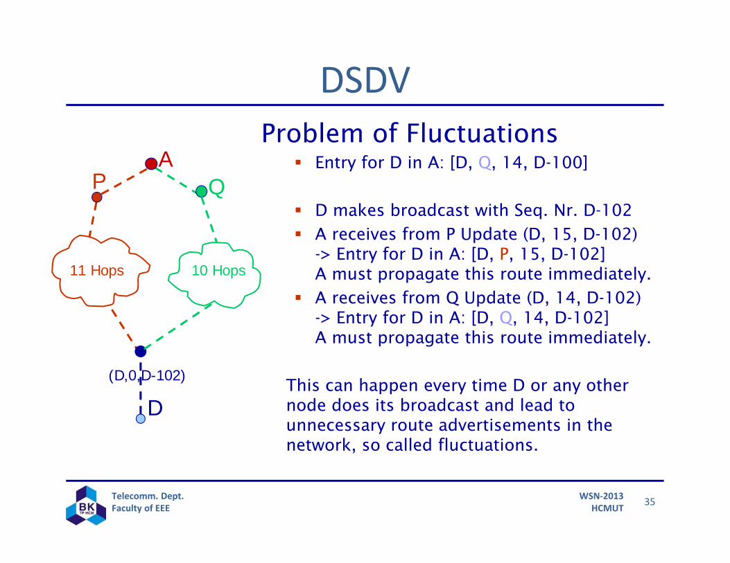
DSDVProblem of Fluctuations

Entry for D in A: [D, Q, 14, D-100]

D makes broadcast with Seq. Nr. D-102 A receives from P Update (D, 15, D-102)

-> Entry for D in A: [D, P, 15, D-102] A must propagate this route immediately.

A receives from Q Update (D, 14, D-102)-> Entry for D in A: [D, Q, 14, D-102]A must propagate this route immediately.

This can happen every time D or any other node does its broadcast and lead to unnecessary route advertisements in the network, so called fluctuations.

A

D

QP

10 Hops11 Hops

(D,0,D-102)


WSN‐2013HCMUT

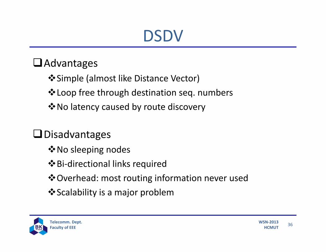
DSDVAdvantagesSimple (almost like Distance Vector)Loop free through destination seq. numbersNo latency caused by route discovery

DisadvantagesNo sleeping nodesBi‐directional links requiredOverhead: most routing information never usedScalability is a major problem


WSN‐2013HCMUT

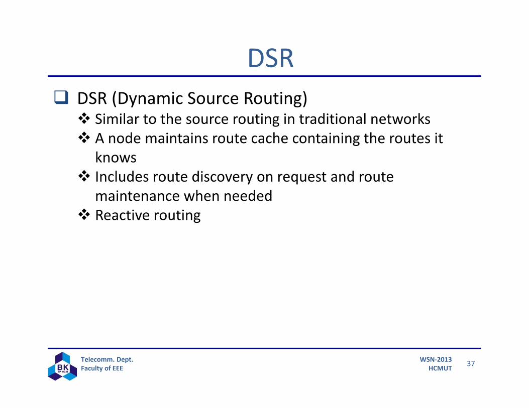
DSR DSR (Dynamic Source Routing) Similar to the source routing in traditional networks A node maintains route cache containing the routes it

knows Includes route discovery on request and route

maintenance when needed Reactive routing


WSN‐2013HCMUT

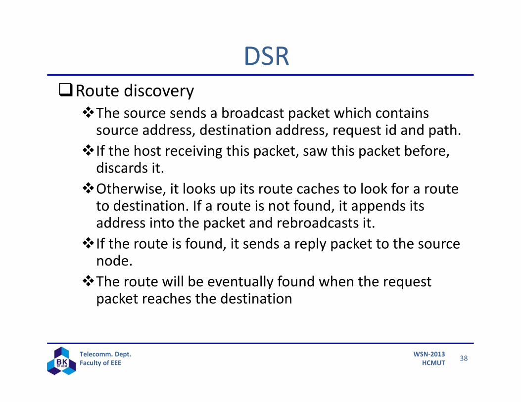
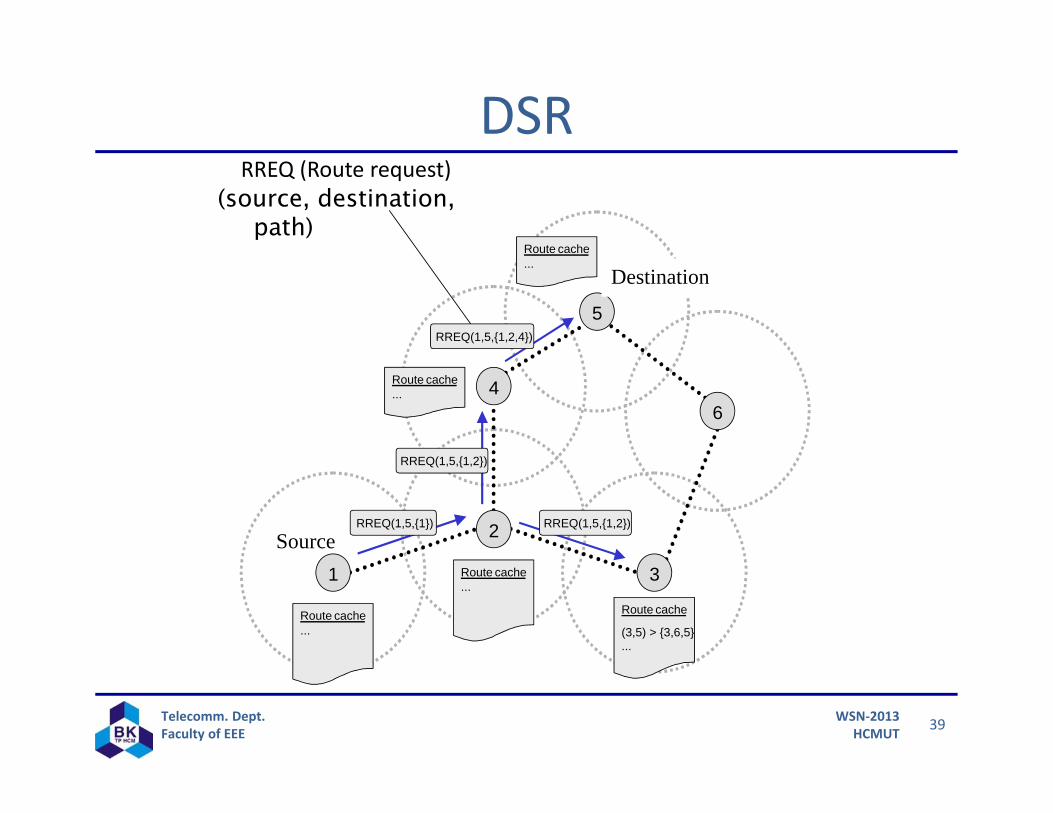
DSRRoute discoveryThe source sends a broadcast packet which contains source address, destination address, request id and path.

If the host receiving this packet, saw this packet before, discards it.

Otherwise, it looks up its route caches to look for a route to destination. If a route is not found, it appends its address into the packet and rebroadcasts it.

If the route is found, it sends a reply packet to the source node.

The route will be eventually found when the request packet reaches the destination


WSN‐2013HCMUT

Source

DSRRREQ (Route request)

4

3

6

5

1

2

RREQ(1,5,{1,2,4})

Route cache

(3,5) > {3,6,5}...

Route cache...

Route cache...

RREQ(1,5,{1})

RREQ(1,5,{1,2})

RREQ(1,5,{1,2})

Route cache...

Route cache...

(source, destination, path)

Destination


WSN‐2013HCMUT

DSRHow to send a reply packet?If the destination has a route to the source in its cache, use it

Else if symmetric links are supported, use the reverse of the route record

Else, if symmetric links are not supported, the destination initiate route discovery to source


WSN‐2013HCMUT

DSR

4

3

6

5

1

2

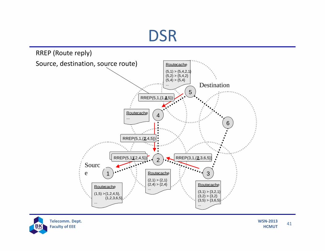
Routecache(3,1) > {3,2,1}(3,2) > {3,2}(3,5) > {3,6,5}...

Routecache...

Routecache(5,1) > {5,4,2,1}(5,2) > {5,4,2}(5,4) > {5,4}...

Routecache(2,1) > {2,1}(2,4) > {2,4}...Routecache

(1,5) >{1,2,4,5},{1,2,3,6,5}

...

RREP(5,1,{1,2,4,5})

RREP(5,1,{1,2,4,5})

RREP(5,1,{1,2,4,5}) RREP(3,1,{1,2,3,6,5})

RREP (Route reply)Source, destination, source route)

Source

Destination


WSN‐2013HCMUT

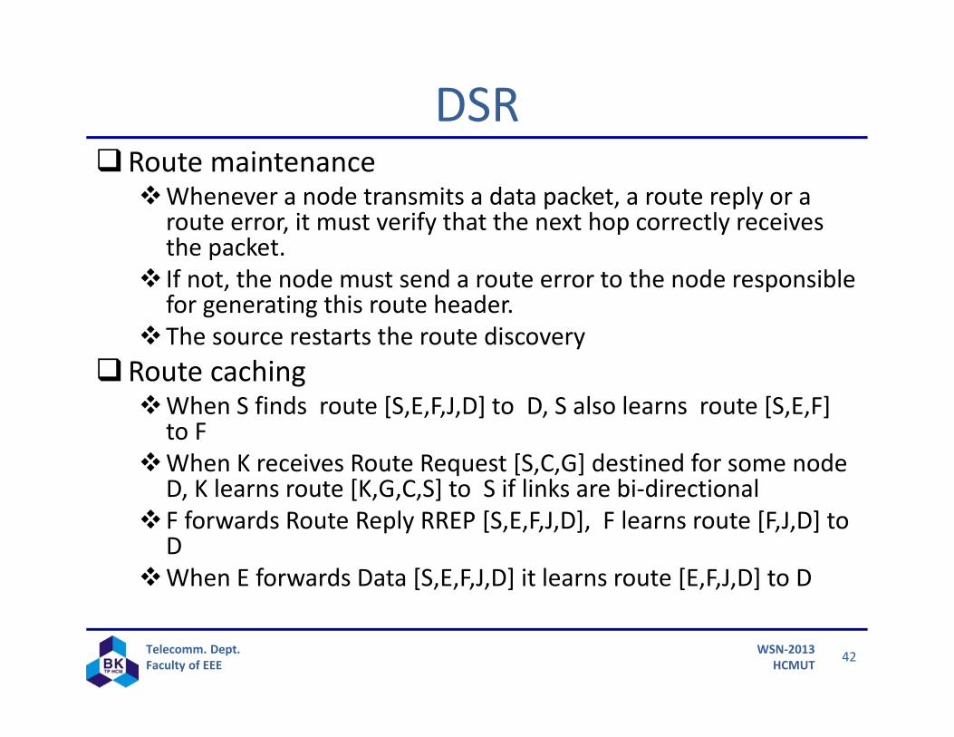
DSRRoute maintenanceWhenever a node transmits a data packet, a route reply or a

route error, it must verify that the next hop correctly receives the packet.

If not, the node must send a route error to the node responsible for generating this route header.

The source restarts the route discoveryRoute cachingWhen S finds route [S,E,F,J,D] to D, S also learns route [S,E,F]

to FWhen K receives Route Request [S,C,G] destined for some node

D, K learns route [K,G,C,S] to S if links are bi‐directionalF forwards Route Reply RREP [S,E,F,J,D], F learns route [F,J,D] to

DWhen E forwards Data [S,E,F,J,D] it learns route [E,F,J,D] to D


WSN‐2013HCMUT

Can Speed up Route Discovery

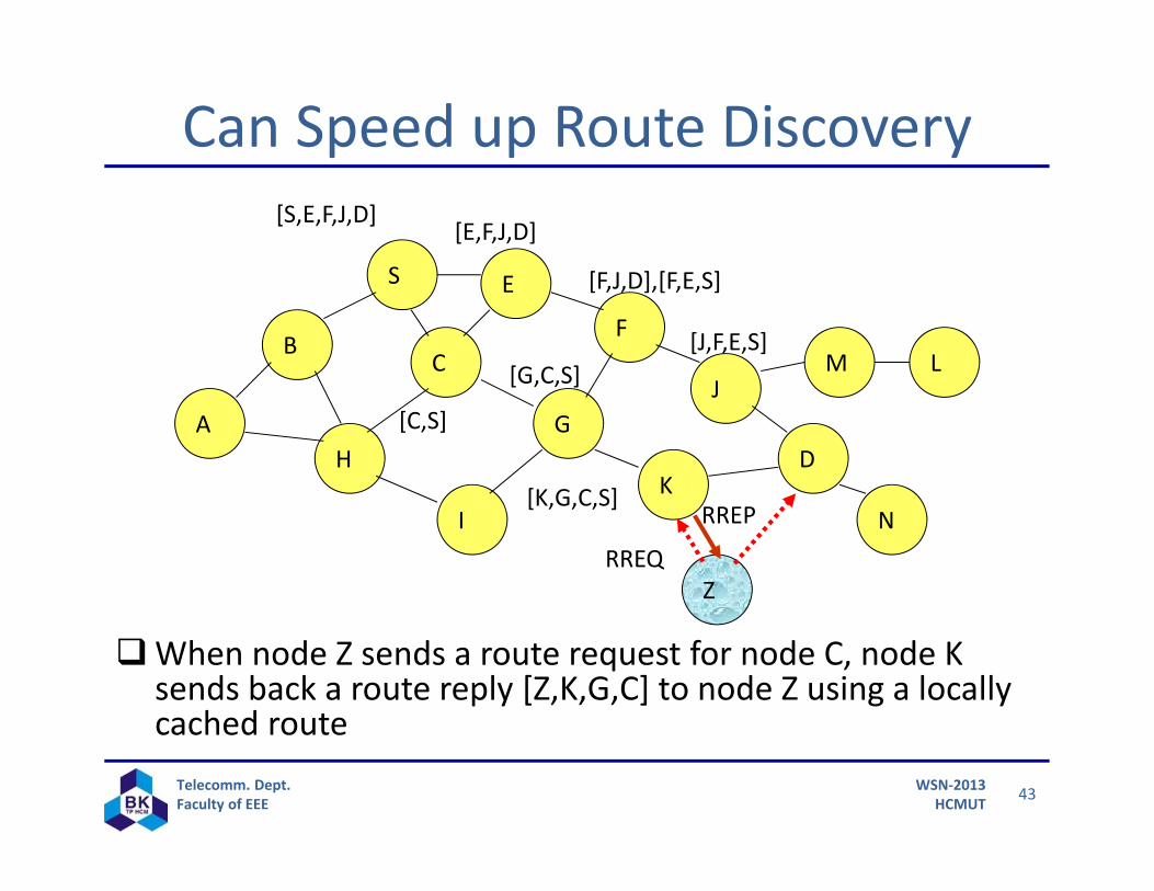
When node Z sends a route request for node C, node K sends back a route reply [Z,K,G,C] to node Z using a locally cached route

B

A

S E

F

H

J

D

C

G

IK

Z

M

N

L

[S,E,F,J,D][E,F,J,D]

[C,S]

[G,C,S]

[F,J,D],[F,E,S]

[J,F,E,S]

RREQ

[K,G,C,S]RREP


WSN‐2013HCMUT

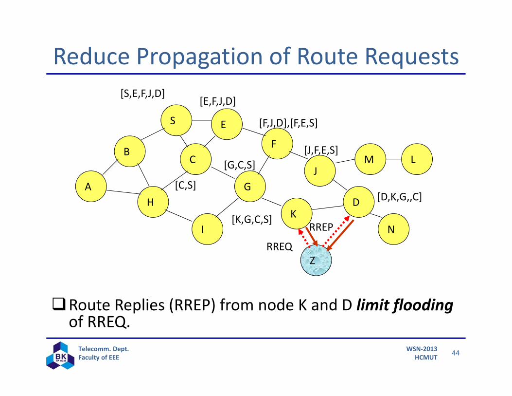
Reduce Propagation of Route Requests

Route Replies (RREP) from node K and D limit flooding of RREQ.

B

A

S E

F

H

J

D

C

G

IK

Z

M

N

L

[S,E,F,J,D][E,F,J,D]

[C,S]

[G,C,S]

[F,J,D],[F,E,S]

[J,F,E,S]

RREQ

[K,G,C,S]RREP

[D,K,G,,C]


WSN‐2013HCMUT

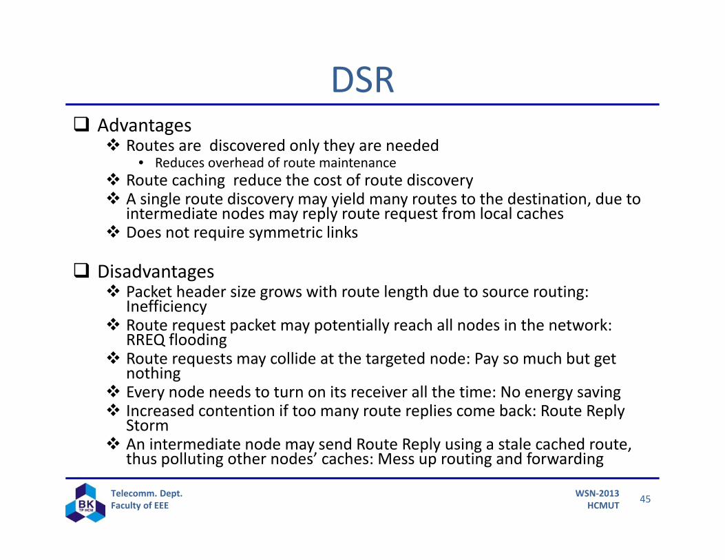
DSR Advantages

Routes are discovered only they are needed• Reduces overhead of route maintenance

Route caching reduce the cost of route discovery A single route discovery may yield many routes to the destination, due to

intermediate nodes may reply route request from local caches Does not require symmetric links

Disadvantages Packet header size grows with route length due to source routing:

Inefficiency Route request packet may potentially reach all nodes in the network:

RREQ flooding Route requests may collide at the targeted node: Pay so much but get

nothing Every node needs to turn on its receiver all the time: No energy saving Increased contention if too many route replies come back: Route Reply

Storm An intermediate node may send Route Reply using a stale cached route,

thus polluting other nodes’ caches: Mess up routing and forwarding


WSN‐2013HCMUT

What’s different in WSN? There is no a priori network graph It is discovered by sending packets and seeing who receives

them.The link relationship is not binary.pairs of nodes communicate with some probability that is

determined by many of factors. It is not static.

The embedding of the “network” in space is important.Need to get information to travel between particular physical

places.But the “communication range” is not a simple function of

distance. addressing & naming Flat EUID? Hierarchical IP? Topologically meaningful? Spatially

meaningful?


WSN‐2013HCMUT

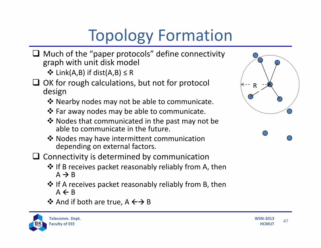
Topology Formation Much of the “paper protocols” define connectivity

graph with unit disk model Link(A,B) if dist(A,B) ≤ R

OK for rough calculations, but not for protocol design Nearby nodes may not be able to communicate. Far away nodes may be able to communicate. Nodes that communicated in the past may not be

able to communicate in the future. Nodes may have intermittent communication

depending on external factors. Connectivity is determined by communication

If B receives packet reasonably reliably from A, then A B

If A receives packet reasonably reliably from B, then A B

And if both are true, A B

R


WSN‐2013HCMUT

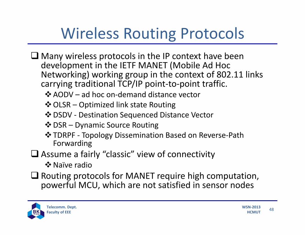
Wireless Routing ProtocolsMany wireless protocols in the IP context have been

development in the IETF MANET (Mobile Ad Hoc Networking) working group in the context of 802.11 links carrying traditional TCP/IP point‐to‐point traffic.AODV – ad hoc on‐demand distance vectorOLSR – Optimized link state RoutingDSDV ‐ Destination Sequenced Distance VectorDSR – Dynamic Source RoutingTDRPF ‐ Topology Dissemination Based on Reverse‐Path

Forwarding Assume a fairly “classic” view of connectivityNaïve radio

Routing protocols for MANET require high computation, powerful MCU, which are not satisfied in sensor nodes


WSN‐2013HCMUT

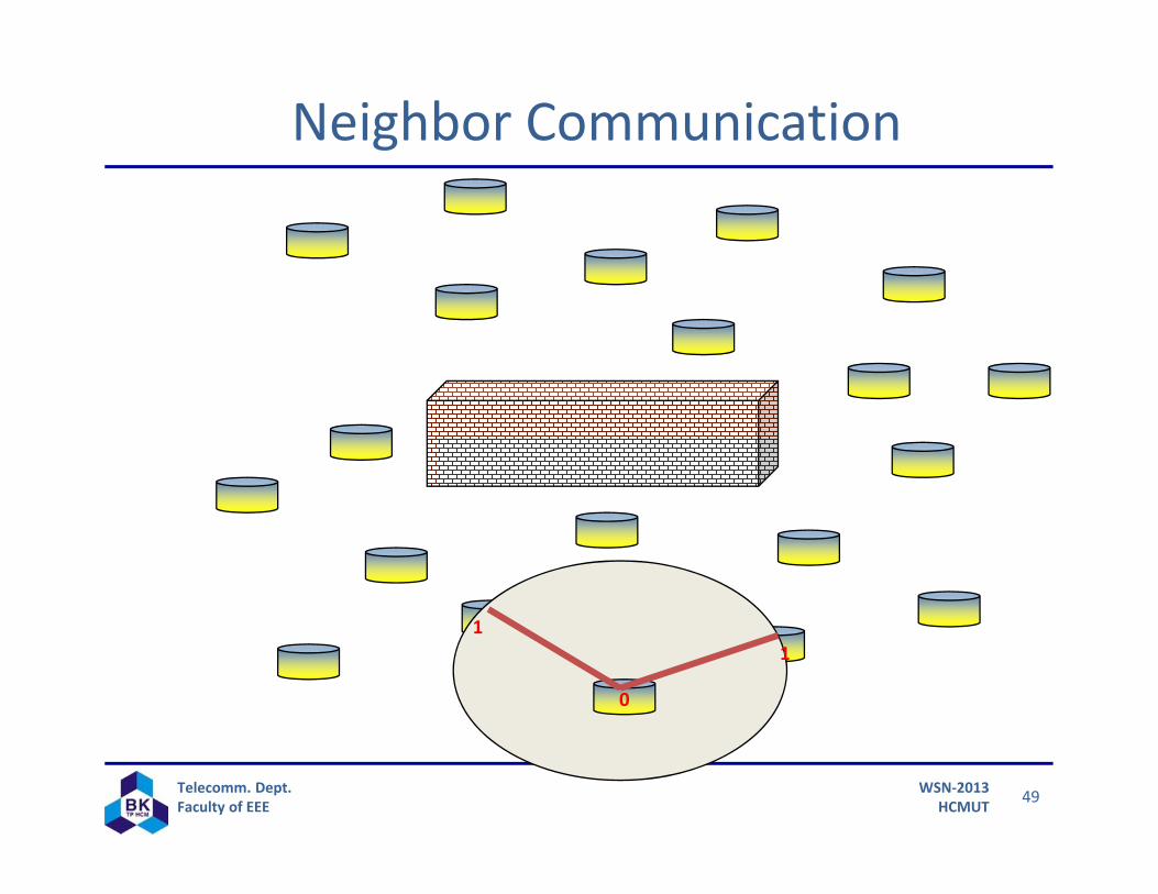
Neighbor Communication

0

11


WSN‐2013HCMUT

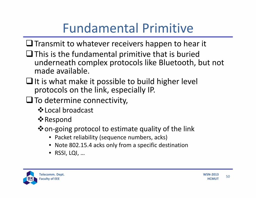
Fundamental PrimitiveTransmit to whatever receivers happen to hear itThis is the fundamental primitive that is buried underneath complex protocols like Bluetooth, but not made available.

It is what make it possible to build higher level protocols on the link, especially IP.

To determine connectivity,Local broadcastRespondon‐going protocol to estimate quality of the link

• Packet reliability (sequence numbers, acks)• Note 802.15.4 acks only from a specific destination• RSSI, LQI, …


WSN‐2013HCMUT

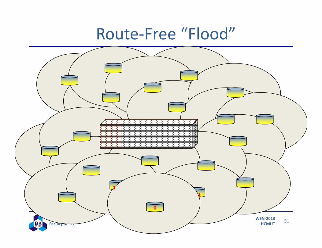
Route‐Free “Flood”

0

11


WSN‐2013HCMUT

“Flooding”Route free dissemination is extremely useful in its own rightDisseminate information

• Router advertisements, solicitations, …Network‐wide discoveryJoin, …

It is also the network primitive that most “ad hoc” protocols used to determine a routeFlood from source till destination is reached.Each node records the source of the flood packet

• This is the parent in the “routing tree”Reverse the links to form the path back


WSN‐2013HCMUT

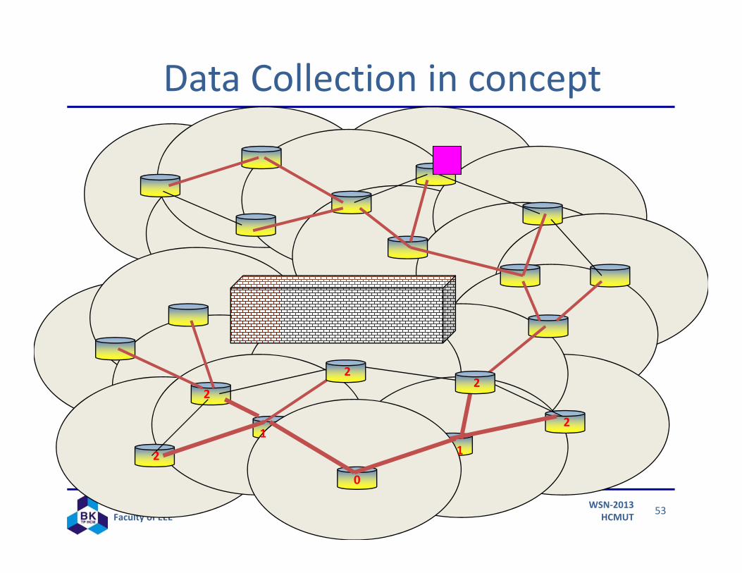
Data Collection in concept

0

112

2

2

22


WSN‐2013HCMUT

The ProblemsFlood causes tremendous contentionMany good links missed because of collisionsHuge amount of noise

Many links are not symmetric


WSN‐2013HCMUT

Trickle – better than floodWant the communication rate per unit area to be constant, regardless of the density of nodesLots of nodes, transmit infrequentlyFew node, transmit more frequently

Nodes listen before transmittingEstimate density based on how many nodes you hear fromArrival during timer wait extends timer

If new value is disseminated by others, no need for you to transmit it.

Increase delay over time so ambient rate approaches zero.

Shorten delay when new epoch appears.


WSN‐2013HCMUT

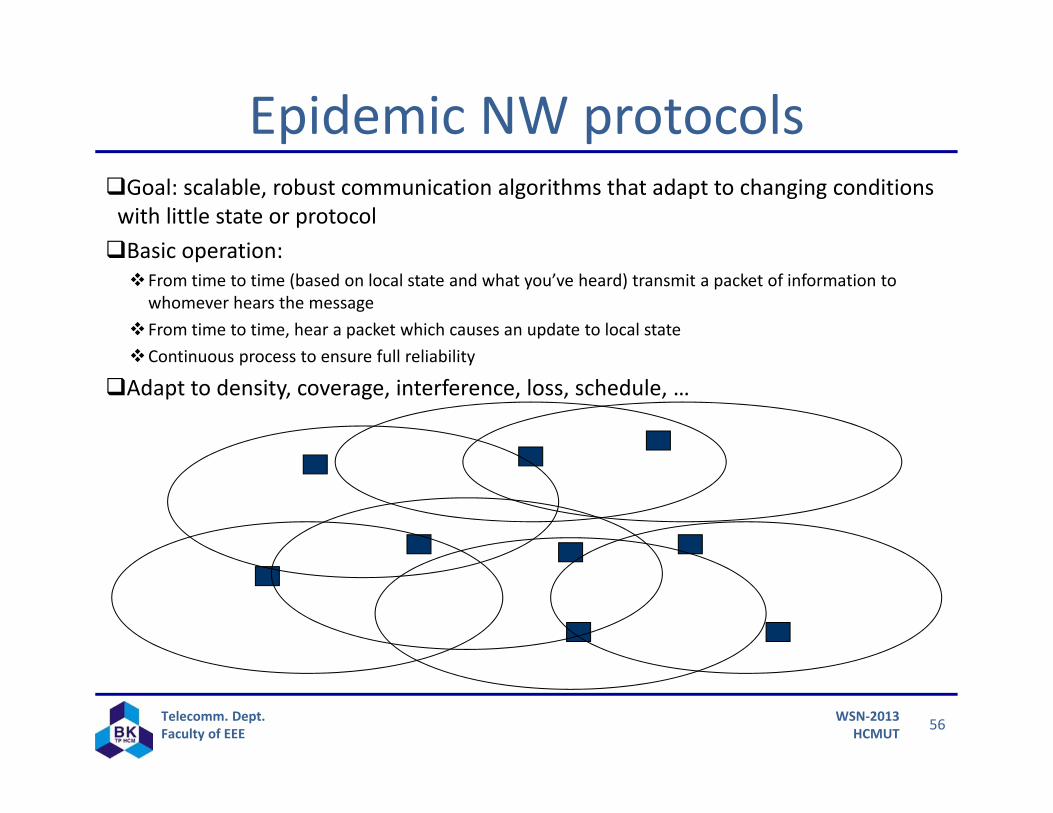
Epidemic NW protocolsGoal: scalable, robust communication algorithms that adapt to changing conditions with little state or protocolBasic operation:From time to time (based on local state and what you’ve heard) transmit a packet of information to whomever hears the message

From time to time, hear a packet which causes an update to local stateContinuous process to ensure full reliability

Adapt to density, coverage, interference, loss, schedule, …


WSN‐2013HCMUT

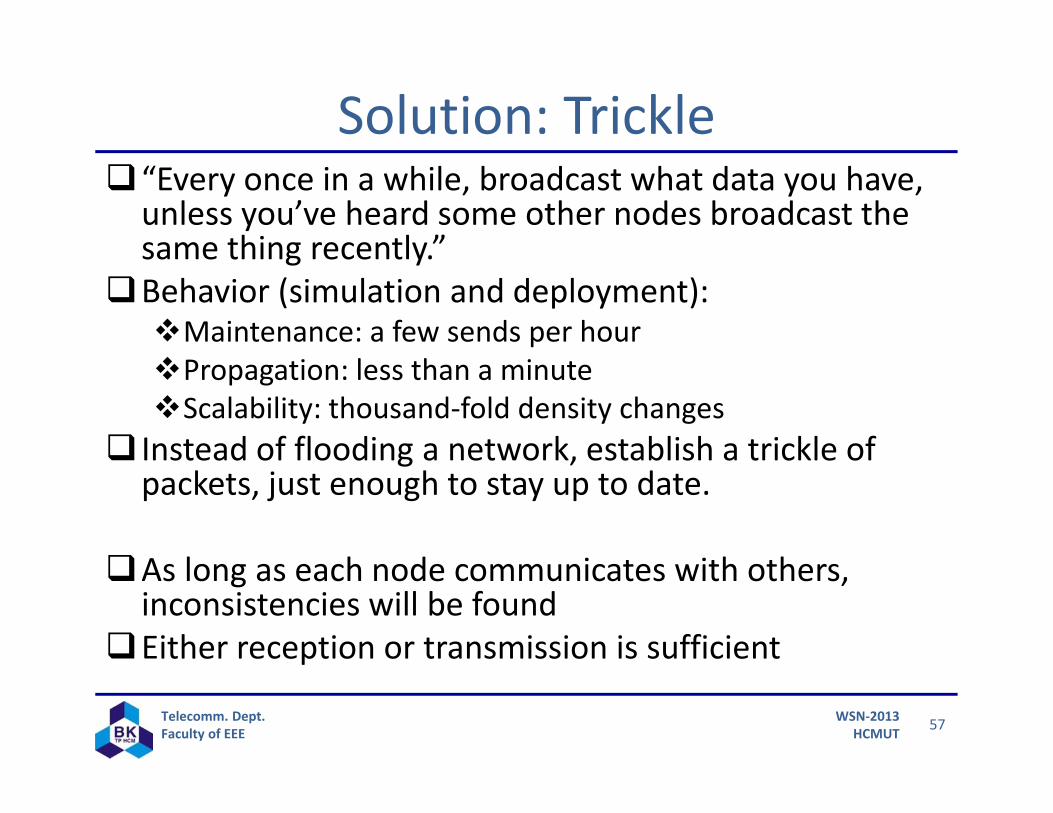
Solution: Trickle“Every once in a while, broadcast what data you have, unless you’ve heard some other nodes broadcast the same thing recently.”

Behavior (simulation and deployment):Maintenance: a few sends per hourPropagation: less than a minuteScalability: thousand‐fold density changes

Instead of flooding a network, establish a trickle of packets, just enough to stay up to date.

As long as each node communicates with others, inconsistencies will be found

Either reception or transmission is sufficient


WSN‐2013HCMUT

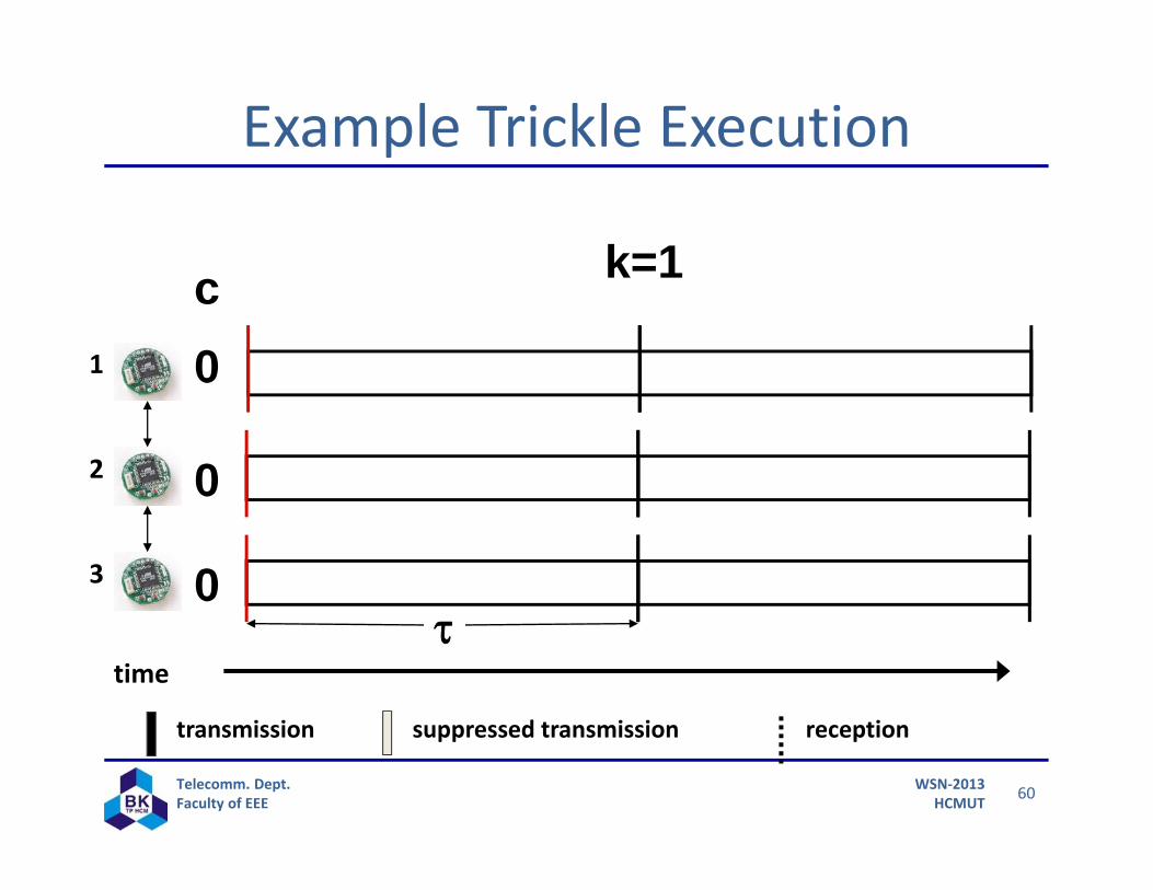
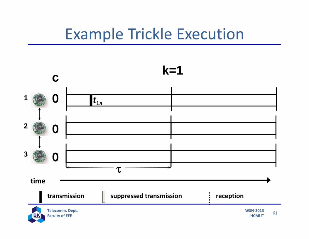
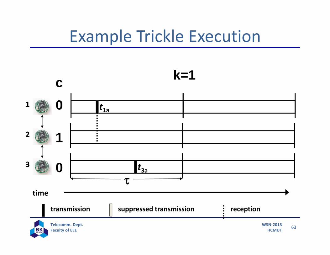
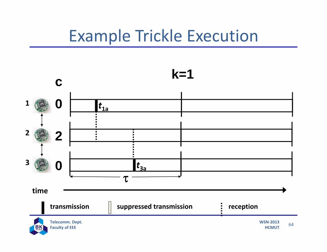
Algorithm Define a desired detection latency, t Choose a redundancy constant k

(receptions + transmissions) <= k In an interval of length t

Trickle keeps the rate as close to k/t as possible

Choose timer t random in (t/2, t] If inconsistent broadcast is heard before t, reset t to tmin.

If c < k consistent broadcasts are heard by t, broadcast Otherwise suppress and double t up to tmax.

When there is nothing new to say, stay quiet


WSN‐2013HCMUTNEST Retreat, Jan 2004 59

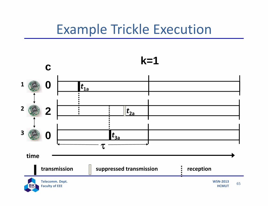
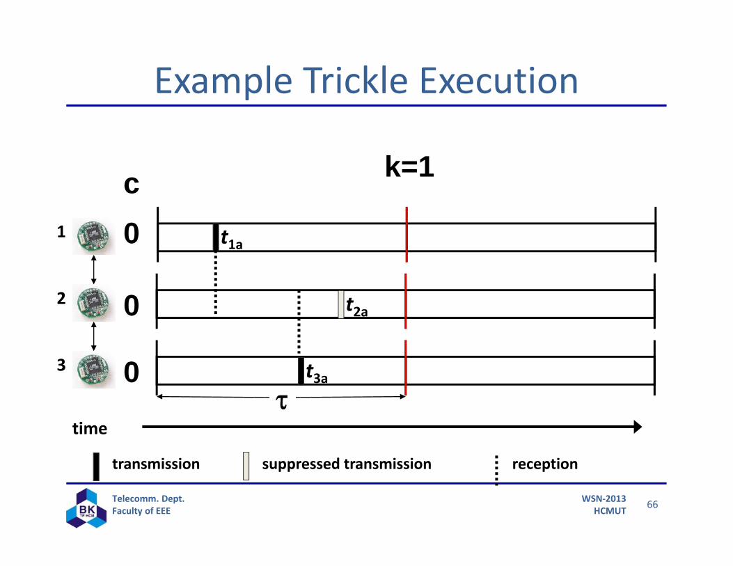
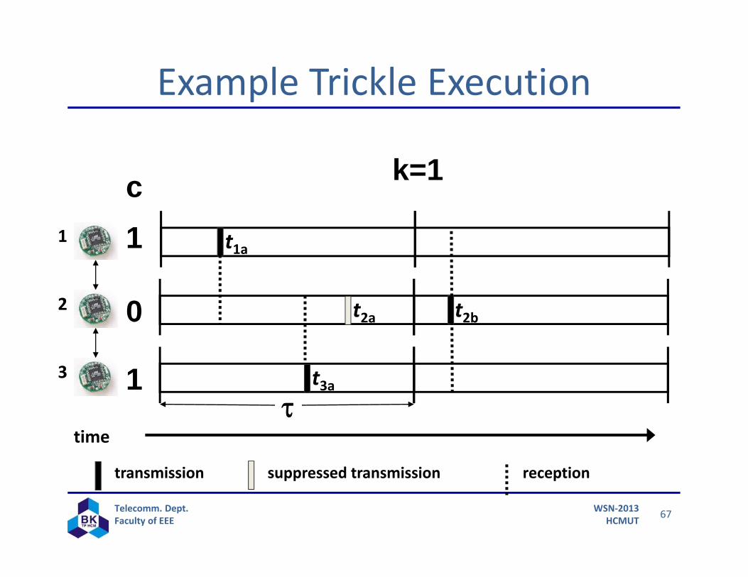
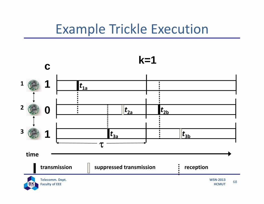
Trickle Algorithm

Time interval of length Redundancy constant k (e.g., 1, 2)

Pick a time t from [0, ]Maintain a counter c, initialized to zeroAt time t, broadcast code metadata if c < kIncrement c when you hear identical metadata to your own

At end of , pick a new t


WSN‐2013HCMUT

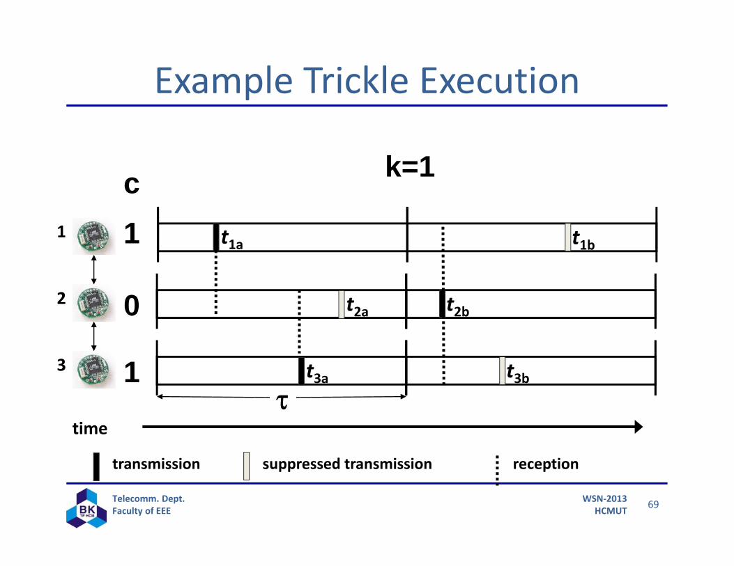
Example Trickle Execution

time

2

3

transmission suppressed transmission reception

1

k=1c0

0

0


WSN‐2013HCMUT


t1a

time

2

3


1

k=1c0

0

0


WSN‐2013HCMUT


t1a

time

2

3


1

k=1c0

1

0


WSN‐2013HCMUT


t1a

time

t3a

2

3


1

k=1c0

1

0


WSN‐2013HCMUT


t1a

time

t3a

2

3


1

k=1c0

2

0


WSN‐2013HCMUT


t1a

time

t2a

t3a

2

3


1

k=1c0

2

0


WSN‐2013HCMUT


t1a

time

t2a

t3a

2

3


1

k=1c0

0

0


WSN‐2013HCMUT


t1a

time

t2a t2b

t3a

2

3


1

k=1c1

0

1


WSN‐2013HCMUT


t1a

time

t2a t2b

t3a t3b

2

3


1

k=1c1

0

1


WSN‐2013HCMUT


t1a t1b

time

t2a t2b

t3a t3b

2

3


1

k=1c1

0

1


WSN‐2013HCMUT

Ideal casek transmissions per intervalFirst k nodes to transmit suppress all othersIndependent of density


WSN‐2013HCMUT

Link Characteristics RSSI/LQI given by hardware How can we consider a link good or bad?

Based on RSSI/LQI? Based on PRR?

Neighbor Management Policy: Add/Remove Information Exchange: Link Estimation Exchange Protocol (LEEP):

measure the link quality based on number of receiving:• Data Packet• Beacon:


WSN‐2013HCMUT

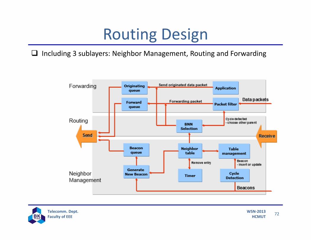
Routing Design Including 3 sublayers: Neighbor Management, Routing and Forwarding


WSN‐2013HCMUT

Simple Address‐Free Flooding ProtocolRoot broadcasts a “new” message to local neighborhood

Each node performs a simple ruleif (“new” incoming msg) then

take local actionretransmit modified msg

No underlying routing structure requiredThe connectivity over physical space determines it.


WSN‐2013HCMUT

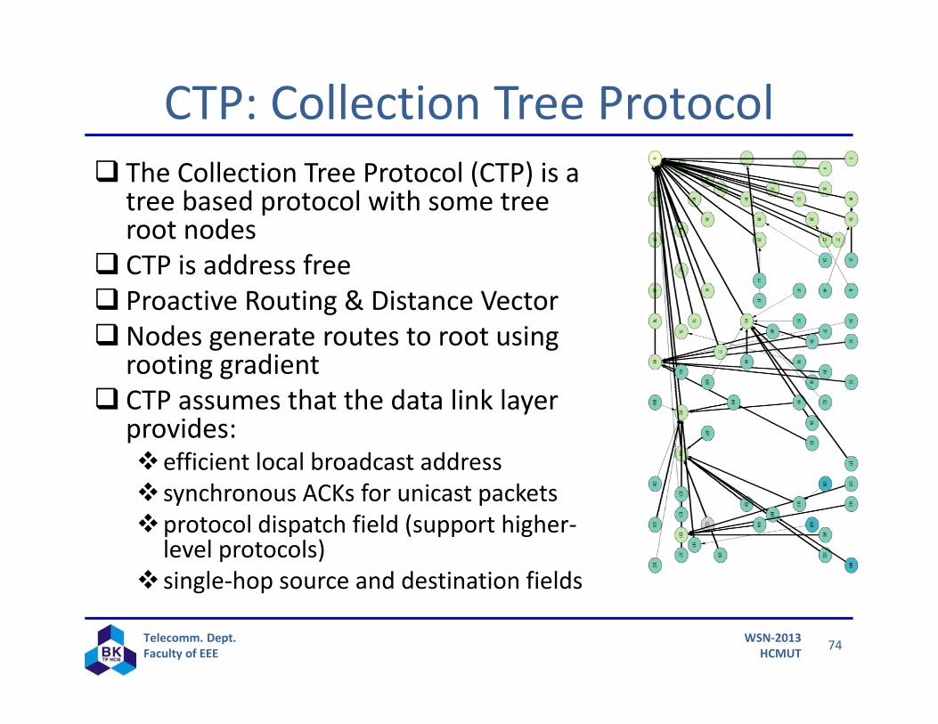
CTP: Collection Tree Protocol The Collection Tree Protocol (CTP) is a

tree based protocol with some tree root nodes

CTP is address free Proactive Routing & Distance VectorNodes generate routes to root using

rooting gradient CTP assumes that the data link layer

provides:efficient local broadcast address synchronous ACKs for unicast packetsprotocol dispatch field (support higher‐

level protocols) single‐hop source and destination fields


WSN‐2013HCMUT

CTP: Collection Tree ProtocolCTP assumes that it has link quality estimates of some number of nearby neighbors

CTP has several mechanisms in order to improve delivery reliability (not promise 100%)

CTP designed for relatively low traffic


WSN‐2013HCMUT

CTP: Routing metric ETX (Expected number of transmission): measure each link’s

delivery probability with broadcast probes (& measure reverse)Pdelivery = Pdata * dACKLink ETX = 1 / PdeliveryRoute ETX = (link ETX)

CTP uses Expected Transmissions (ETX) as a routing metricETXroot=0 and ETXnode=ETXparent+ETXlinktoparentCTP should choose the route with the lowest ETXCTP represents ETX as 16‐bit fix‐point real number with precision of hundredths

Two main problemRooting loopsPacket duplication


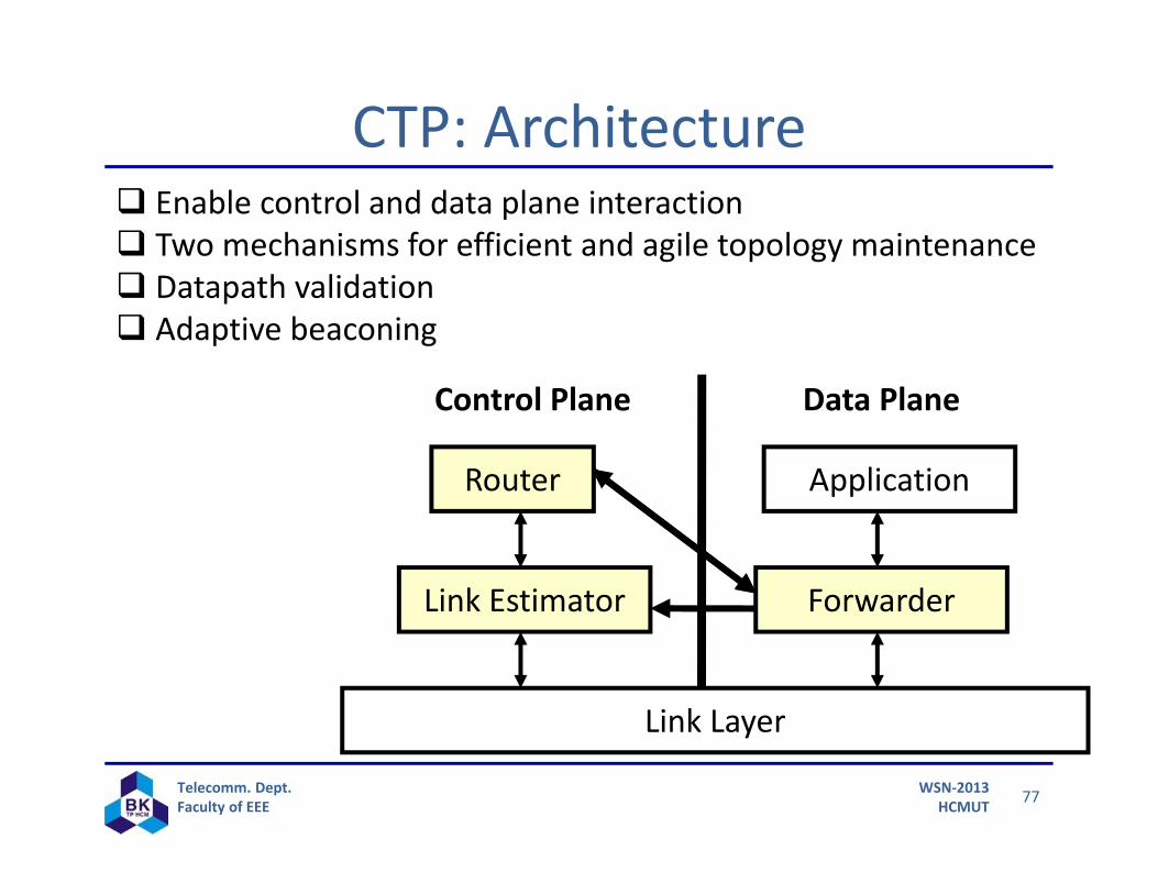
WSN‐2013HCMUT

CTP: Architecture Enable control and data plane interaction Two mechanisms for efficient and agile topology maintenance Datapath validation Adaptive beaconing

Router

ForwarderLink Estimator

Link Layer

Application

Control Plane Data Plane


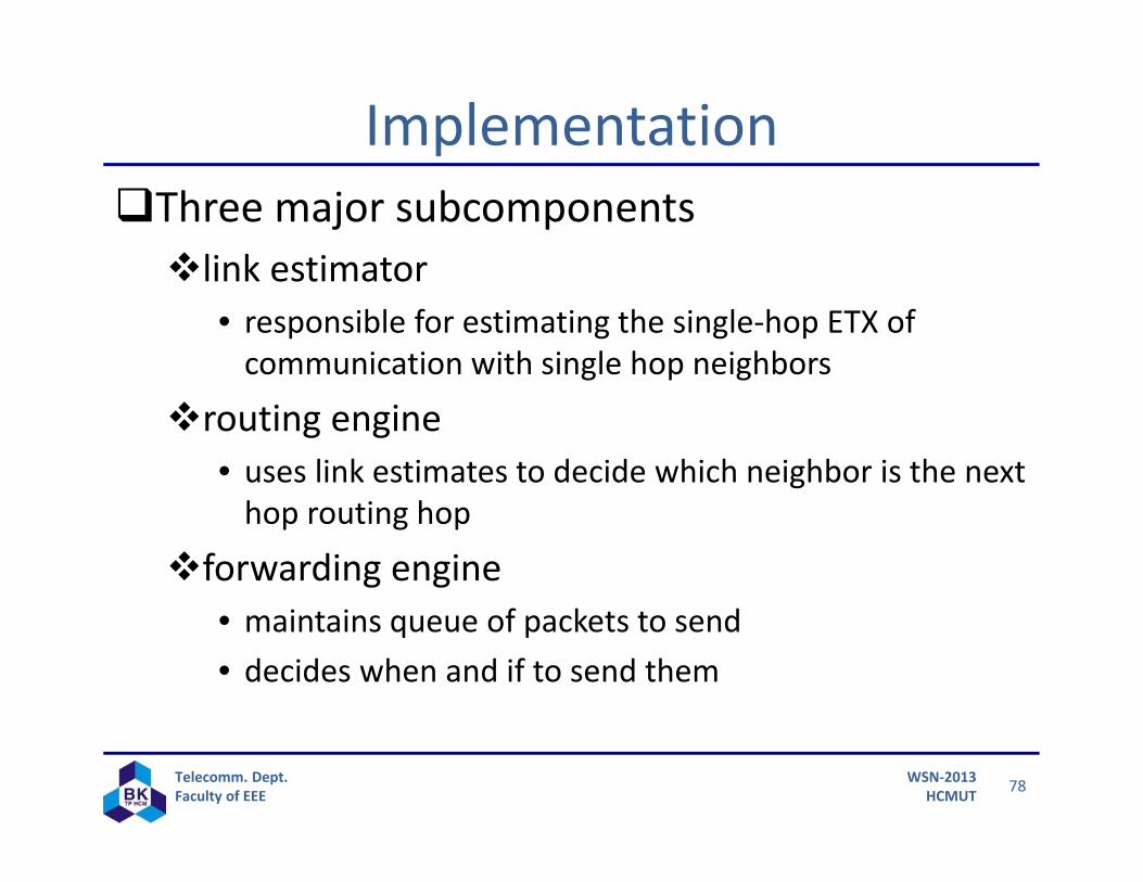
WSN‐2013HCMUT

ImplementationThree major subcomponentslink estimator

• responsible for estimating the single‐hop ETX of communication with single hop neighbors

routing engine• uses link estimates to decide which neighbor is the next hop routing hop

forwarding engine• maintains queue of packets to send• decides when and if to send them


WSN‐2013HCMUT

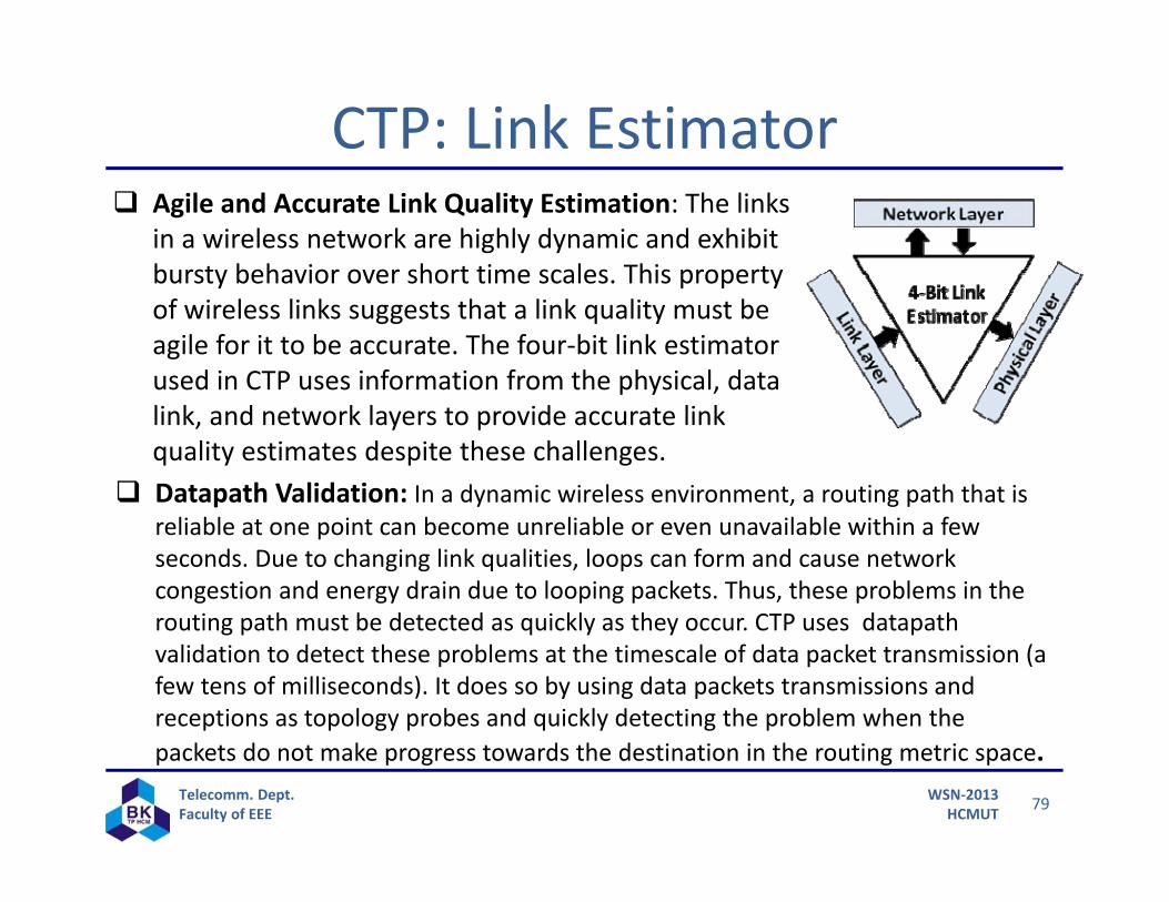
CTP: Link Estimator Agile and Accurate Link Quality Estimation: The links

in a wireless network are highly dynamic and exhibit bursty behavior over short time scales. This property of wireless links suggests that a link quality must be agile for it to be accurate. The four‐bit link estimator used in CTP uses information from the physical, data link, and network layers to provide accurate link quality estimates despite these challenges.

Datapath Validation: In a dynamic wireless environment, a routing path that is reliable at one point can become unreliable or even unavailable within a few seconds. Due to changing link qualities, loops can form and cause network congestion and energy drain due to looping packets. Thus, these problems in the routing path must be detected as quickly as they occur. CTP uses datapathvalidation to detect these problems at the timescale of data packet transmission (a few tens of milliseconds). It does so by using data packets transmissions and receptions as topology probes and quickly detecting the problem when the packets do not make progress towards the destination in the routing metric space.


WSN‐2013HCMUT

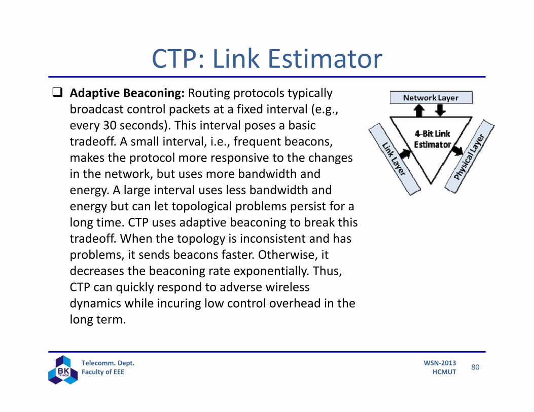
CTP: Link Estimator Adaptive Beaconing: Routing protocols typically

broadcast control packets at a fixed interval (e.g., every 30 seconds). This interval poses a basic tradeoff. A small interval, i.e., frequent beacons, makes the protocol more responsive to the changes in the network, but uses more bandwidth and energy. A large interval uses less bandwidth and energy but can let topological problems persist for a long time. CTP uses adaptive beaconing to break this tradeoff. When the topology is inconsistent and has problems, it sends beacons faster. Otherwise, it decreases the beaconing rate exponentially. Thus, CTP can quickly respond to adverse wireless dynamics while incuring low control overhead in the long term.


WSN‐2013HCMUT

Routing EnginePicking the next hop for data transmissionKeeps track of the path ETX of the subset of the nodes

The minimum cost route has the smallest sumthe path ETX from that nodethe link ETX of that node


WSN‐2013HCMUT

Forwarding EngineTransmitting, retransmitting packets to the next hop and passing ACK based information to the link estimator

Deciding when to transmit packets to the next hopDetecting routing inconsistencies and informing the routing engine

Maintaining a queue of packets to transmit (local and forwarded)

Detection singe‐hop transmission duplicates


WSN‐2013HCMUT

CTP: SummaryAdvantagesConsistent routingSuitable for many‐to‐one applicationHigh PRR

DisadvantagesAny‐to‐any routing (e.g. IP application)

Documents

Ch06-Routing in WSNs