Chapter 12 Combinatorics - Yale University · Chapter 12 Combinatorics ... SECTION 5 establishes a connection between VC dimension and packing ... can also be applied to collections

Chapter 12

Combinatorics

SECTION 1 presents a simple concrete example to illustrate the use of the combinatorialmethod for deriving bounds on packing numbers.

SECTION 2 defines the concept of shatter dimension, for both classes of sets andbinary matrices, and the VC dimension for a class of sets.

SECTION 3 derives the general combinatorial bound (the VC lemma) relating theshatter dimension to the number of distinct patterns picked out. The proof of themain theorem introduces the important technique known as downshifting.

SECTION 4 describes ways to create VC classes of sets, including methods based on

o-minimality. incomplete

SECTION 5 establishes a connection between VC dimension and packing numbers forVC subgraph classes of functions under an L1 metric.

Unedited fragments from here on

SECTION 6 fat shatteringSECTION 7 Mendelson & VSECTION 8 Haussler & LongSECTION 9 presents a refinement of the calculation from Section 5, leading to a

sharper bound for packing numbers. The result is included mainly for its aestheticappeal and for the sake of those who like to see best constants in inequalities.

1. An introductory example

Suppose F := {x1, . . . , xn} is a finite subset of some X and D is some collectionof subsets of X. A set D from D is said to pick out the points {xi : i ∈ J},where J ⊆ {1, 2, . . . , n}, if {

xi ∈ D for i ∈ J

xi ∈ Dc for i ∈ Jc

The class D is said to shatter F if it can pick out all 2n possible subsets of F .The combinatorial argument often referred to as the VC method (in honor

of the important contributions of Vapnik & Cervonenkis) provides a bound onthe number of different subsets that can be picked out from a given F in termsof the size of the largest subset F0 of F that D can shatter. The combinatorialbound also leads to uniform bounds on the covering numbers of D as a subsetof L1(P), as P ranges over probability measures carried by X. The methodscan also be applied to collections of real-valued functions on X, leading tobounds on Lα(P) covering numbers for a wide range of α values, includingα = 1 and α = 2. These bounds can then be fed into chaining arguments

27 March 2005 Asymptopia, version: 27mar05 c©David Pollard 1

2 Chapter 12: Combinatorics

to obtain maximal inequalities for some processes indexed by collections offunctions on X.

The VC method is elegant and leads to results not easily obtained in otherways. The basic calculations occupy only a few pages. Nevertheless, the ideasare subtle enough to appear beyond the comfortable reach of many would-beusers. With that fact in mind, I offer a preliminary more concrete example, inthe hope that the idea might seem less mysterious.

Remark. You will notice that I make no effort to find the best upperbound. In fact, as will become clear later, any bound that grows like apolynomial in the size of the subset leads to the same sort of bound on thecovering numbers.

Consider the class H2 of all closed half-spaces in R2. Let F be a set of npoints in R2. How many distinct subsets are there of the form H ∩ F , with Hin H2? Certainly there can be no more than 2n , because F has only that manysubsets.

Define FH2 = {F ∩ H : H ∈ H2}, and let #FH2 be its cardinality. A simpleargument will show that #FH2 ≤ 4n2. Indeed, consider a particular nonemptysubset F0 of F picked out by a particular half-space H0. There is no loss ofgenerality in assuming that at least one point x0 of F0 lies on L0, the boundaryof H0: otherwise we could replace H0 by a smaller H1 whose boundary runsparallel to L0 through the point of F0 closest to L0.

As seen from x0, the other n − 1 points of F all lie on a set L(x0) of atmost n − 1 lines through x0. Augment L(x0) by another set L′(x0) of at most

n − 1 lines through x0, one in each angle between two linesfrom L(x0). The lines in L(x0) ∪ L′(x0) define a collectionof at most 4(n − 1) closed half-spaces, each with x0 on itsboundary. The collection ∪x0∈FH2(x) accounts for all possiblenonempty subsets of F picked out by closed half-spaces. Thusthere are at most

1 + 4n(n − 1) ≤ 4n2

subsets that can be picked out from F by H2. The extra 1 takes care of theempty set.

The slow increase in #FH2 , at an O(n2) rate rather than a rapid 2n rate,has an unexpected consequence for the packing numbers of H2 when equippedwith an L1(P) (pseudo)metric for some probability measure P on the Borelsigma-field.

Remark. In fact, we will only need the bound when P concentrateson a finite number of points, in which case all measurability difficultiesdisappear.

The result is surprising because it makes no regularity assumptions about theprobability measure P . The argument is due to Dudley (1978), who created thegeneral theory for abstract empirical processes.

The L1(P) distance between two (measurable) sets B and B ′ is defined as

P|B − B ′| = P(B�B ′),

the probability measure of the symmetric difference. Say that the two sets areε-separated if P(B�B ′) > ε. The packing number π1(ε) := D(ε, H2, L

1(P))

is defined as the largest N for which there exists a collection of N closedhalf-spaces, each pair ε-separated. We can use the polynomial bound for #FH2

to derive an upper bound for the packing numbers, by means of a cunninglychosen F .

2 27 March 2005 Asymptopia, version: 27mar05 c©David Pollard

12.1 An introductory example 3

Suppose there exist half-spaces H1, H2, . . . , HN for which P(Hi�Hj ) > ε

for i �= j . The trick is to find a set F of m = 2 log N/ε points from which eachHi picks out a different subset. (For simplicity, I am ignoring the possibilitythat this m might not be an integer. A more precise calculation will be givenin Section 5.) Then H2 will pick out at least N subsets from the m points, andthus

N ≤ 4

(2 log N

ε

)2

If we bound log N by a constant multiple of N 1/4, then solve the inequalityfor N , we get an upper bound N ≤ O(1/ε)4. With a smaller power in thebound for log N we would bring the power of 1/ε arbitrarily close to 2.

With a little more work, the bound can even be brought to the formC2(ε

−1 log(1/ε))2, at least for ε bounded away from 1. At this stage there islittle point in struggling to get the best bound in ε. The qualitative consequencesof the polynomial bound in 1/ε are the same, no matter what the degree of thepolynomial.

How do we find a set F0 = {x1, . . . , xm} of points in R2 from which eachHi picks out a different subset? We need to place at least one point of F0 ineach of the

(N2

)symmetric differences Hi�Hj . It might seem we are faced

with a delicate task involving consideration of all possible configurations of thesymmetric differences, but here probability theory comes to the rescue.

Generate F0 as a random sample of size m from P . If m ≥ 2 log N/ε, thenthere is a strictly positive probability that the sample has the desired property.Indeed, for fixed i �= j ,

P{Hi and Hj pick out same points from F0}= P{no points of sample in Hi�Hj }= (1 − P(Hi�Hj ))

m

≤ (1 − ε)m

≤ exp(−mε).

Add up(N

2

)such probability bounds to get a conservative estimate,

P{no pair Hi , Hj pick same subset from F0} ≤ (N2

)exp(−mε).

When m = 2 log N/ε the last bound is strictly less than 1, as desired.Probability theory has been used to prove an existence result, which gives

a bound for a packing number, which will be used to derive probabilisticconsequences—all based ultimately on the existence of the polynomial boundfor #FH2 .

The class H2 might shatter some small F sets. For example, if F consistsof 3 points, not all on the same straight line, then it can be shattered by H2.However no set of 9 points can be shattered, because there are 29 = 512possible subsets—the empty set included—whereas the half-spaces can pickout at most 4 × 92 = 324 subsets. More generally, 2n > 4n2 for all n ≥ 9, sothat, of course, no set of more than 9 points can be shattered by H2.

Remark. You should find it is easy to improve on the 9, by arguingdirectly that no set of 4 points can be shattered by H2. Indeed, if H2 picksout both F1 and F2 = Fc

1 , then the convex hulls of F1 and F2 must bedisjoint. You have only to demonstrate that from every F with at least 4points, you can find such F1 and F2 whose convex hulls overlap.

In summary: The size of the largest set shattered by H2 is 3. Note wellthat the assertion is not that all sets of 3 points can be shattered, but merelythat there is some set of 3 points that is shattered, while no set of 4 points can



be shattered. In the terminology of Section 2, the class H2 would be said tohave VC dimension equal to 3.

The argument had little to do with the choice of H2 as a class of half-spacesin a particular Euclidean space. It would apply to any class D for which #FD

is bounded by a fixed polynomial in #F . And therein lies the challenge. Ingeneral, for more complicated classes of subsets D of arbitrary spaces, it can bequite difficult to bound #FD by a polynomial in #F , but it is often less difficultto prove existence of a finite VC-dim such that no set of more than VC-dimpoints can be shattered by D. The miracle is that a polynomial bound thenfollows automatically, as will be shown in Section 2.

I need to check the assertions in the following Remark. See Dudley (1978,Section 7).

Remark. For the set Hk of all closed halfspaces in Rk , the VC methodwill deliver a bound

N ≤ p(n) =∑

j≤k+1

(n

j

)for the largest number of subsets that can be picked out from a set with npoints. For k = 2, the bound is a cubic in n, which is inferior (for large n)to the 4n2 obtained above. In fact, there is an even better bound,

N ≤ p(n) = 2∑

j≤k

(n − 1

j

)which is achieved when no k + 1 of the points lie in any hyperplane. Fork = 2, the bound becomes n2 − n + 2.

The upper bound, p(n), for the number of subsets picked out from aset of n points, should not be confused with∑

j≤k

(N

j

),

the largest number of regions into which Rk can be partitioned by Nhyperplanes.

2. Shattered subsets, shattered columns of a matrix

There are various ways to express the counting arguments that lead the boundson the number of subsets picked out by a given D from a finite subset. Actually,when the subset is generated as a random sample from some distribution, it isbetter to allow for possible duplicates by counting patterns picked out froman x = (x1, . . . , xn) in Xn . A pattern is specified by a subset J of {1, 2, . . . , n}and a set DJ from D for which

<1>

{xi ∈ DJ for i ∈ J

xi ∈ DcJ

for i ∈ Jc

Of course, the DJ need not be unique. In general, there will be many different D

sets that pick out the same pattern from x. For counting purposes, we canidentify a D that picks out N distinct patterns from x with an N × n binarymatrix V = Vx,D, that is a matrix with distinct rows with {0, 1} entries. Thesubset J from <1> would correspond to row of the matrix with a 1 in thecolumns picked out by J and 0 elsewhere. We could also identify each row ofthe matrix with a different vertex of {0, 1}n .


12.2 Shattered subsets, shattered columns of a matrix 5

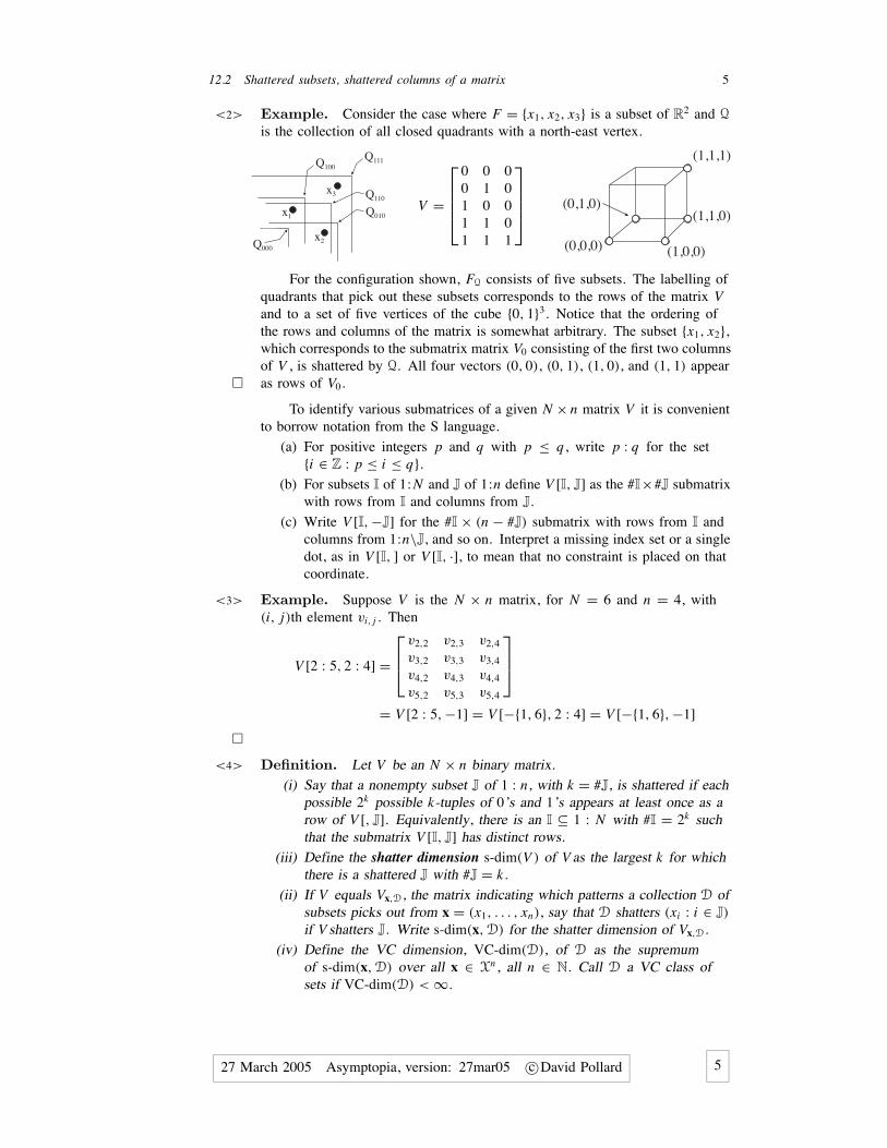
<2> Example. Consider the case where F = {x1, x2, x3} is a subset of R2 and Q

is the collection of all closed quadrants with a north-east vertex.

Q111

Q110

Q100

Q010

Q000

x1

x2

x3

V =

⎡⎢⎢⎢⎣

0 0 00 1 01 0 01 1 01 1 1

⎤⎥⎥⎥⎦

(0,0,0) (1,0,0)

(0,1,0)(1,1,0)

(1,1,1)

For the configuration shown, FQ consists of five subsets. The labelling ofquadrants that pick out these subsets corresponds to the rows of the matrix Vand to a set of five vertices of the cube {0, 1}3. Notice that the ordering ofthe rows and columns of the matrix is somewhat arbitrary. The subset {x1, x2},which corresponds to the submatrix matrix V0 consisting of the first two columnsof V , is shattered by Q. All four vectors (0, 0), (0, 1), (1, 0), and (1, 1) appearas rows of V0.�

To identify various submatrices of a given N × n matrix V it is convenientto borrow notation from the S language.

(a) For positive integers p and q with p ≤ q, write p : q for the set{i ∈ Z : p ≤ i ≤ q}.

(b) For subsets I of 1:N and J of 1:n define V [I, J] as the #I×#J submatrixwith rows from I and columns from J.

(c) Write V [I, −J] for the #I × (n − #J) submatrix with rows from I andcolumns from 1:n\J, and so on. Interpret a missing index set or a singledot, as in V [I, ] or V [I, ·], to mean that no constraint is placed on thatcoordinate.

<3> Example. Suppose V is the N × n matrix, for N = 6 and n = 4, with(i, j)th element vi, j . Then

V [2 : 5, 2 : 4] =

⎡⎢⎣

v2,2 v2,3 v2,4

v3,2 v3,3 v3,4

v4,2 v4,3 v4,4

v5,2 v5,3 v5,4

⎤⎥⎦

= V [2 : 5, −1] = V [−{1, 6}, 2 : 4] = V [−{1, 6}, −1]

�<4> Definition. Let V be an N × n binary matrix.

(i) Say that a nonempty subset J of 1 : n, with k = #J, is shattered if eachpossible 2k possible k-tuples of 0’s and 1’s appears at least once as arow of V [, J]. Equivalently, there is an I ⊆ 1 : N with #I = 2k suchthat the submatrix V [I, J] has distinct rows.

(iii) Define the shatter dimension s-dim(V ) of V as the largest k for whichthere is a shattered J with #J = k.

(ii) If V equals Vx,D, the matrix indicating which patterns a collection D ofsubsets picks out from x = (x1, . . . , xn), say that D shatters (xi : i ∈ J)

if V shatters J. Write s-dim(x, D) for the shatter dimension of Vx,D.(iv) Define the VC dimension, VC-dim(D), of D as the supremum

of s-dim(x, D) over all x ∈ Xn , all n ∈ N. Call D a VC class ofsets if VC-dim(D) < ∞.



<5> Example. The matrix

V =

⎡⎢⎢⎢⎢⎢⎣

1 0 0 00 1 1 01 0 0 10 1 0 10 0 1 11 0 1 1

⎤⎥⎥⎥⎥⎥⎦

does not shatter {1, 2} because the vector (1, 1) does not appear as a rowof the 6 × 2 submatrix V [, {1, 2}], the first two columns of V . Each ofthe other five subsets of {1, 2, 3, 4} of size two is shattered. For example,V [{1, 2, 4, 5}, {2, 3}] has distinct rows. No subset of three (or four) columnsis shattered. Each singleton {1}, {2}, {3}, and {4} is shattered, because eachcolumn contains at least one 0 and one 1. (Easier: every nonempty subset of ashattered J is also shattered.)

The matrix V has shatter dimension s-dim(V ) equal to 2. For futurereference, note that the number of rows is strictly greater than

(40

) + (41

).�

<6> Example. For the class Hk of all closed half-spaces in Rk , show thatVC-dim(Hk) ≤ k + 1.

It is easy to verify that Hk shatters the k +1 points consisting of the originand the k unit vectors that make up the usual basis: consider sets of the form{x : α · x ≤ c} for various α with components 0 or ±1.

It remains to show that Hk can shatter no set F = {x0, . . . , xk+1} of k + 2points in Rk . Linear dependence of the vectors x1 − x0, . . . , xk+1 − x0 ensuresexistence of coefficients αi , not all zero, such that∑k+1

i=1αi (xi − x0) = 0.

Put α0 = − ∑k+1i=1 αi . Then

∑k+1i=0 αi = 0 and

∑k+1i=0 αi xi = 0, or∑k+1

i=0α+

i xi =∑k+1

i=0α−

i xi .

Divide through by the nonzero quantity∑k+1

i=0 α+i = ∑k+1

i=0 α−i to recognize that

we have found disjoint subsets F0 and F1 of F whose convex hulls overlap.There can be no closed half-space that picks out F0 from F , for the existenceof such a half-space would imply that the convex hull of F0 is disjoint from theconvex hull of F\F0: a contradiction.�

<7> Example. Suppose F is a k-dimensional vector space of functions on X.Write D for the class of all sets of the form { f ≥ 0}, with f in F. Show thatVC-dim(D) ≤ k.

Consider a set of k + 1 points x0, . . . , xk in X. The set F of points of theform

( f (x0), . . . , f (xk)) for f in F

is a vector subspace of Rk+1 of dimension at most k. There must exist somenonzero vector α orthogonal to F. Express the orthogonality as

k∑i=0

α+i f (xi ) =

k∑i=0

α−i f (xi ) for each f in F.

Without loss of generality suppose α0 > 0. No member of D can pick out thesubset {xi : αi < 0}: if f (xi ) ≥ 0 when αi < 0 and f (xi ) < 0 when αi ≥ 0then the left-hand side of the equality would be strictly negative, while theright-hand side would be nonnegative. The class D has shatter dimension atmost k; it shatters no set of k + 1 or more points.�


12.3 The VC lemma for binary matrices 7

3. The VC lemma for binary matrices

The key result in the area is often called the VC lemma, although credit shouldbe spread more widely. (See the Notes in Section 11.)

<8> Theorem. Let V be an N × n binary matrix. If s-dim(V ) ≤ d then

N ≤(

n

0

)+

(n

1

)+ . . . +

(n

d

).

If n ≥ d , the upper bound is less than (en/d)d .

Proof. I will establish the contrapositive, by showing that if

<9> N >

(n

0

)+

(n

1

)+ . . . +

(n

d

)then s-dim(V ) > d.

Define the downshift for the j th column of the matrix as the operation:

for i = 1, . . . , Nif V [i, j] = 1 change it to a 0 unless the resultingmatrix V (1) would no longer have distinct rows

For example, the downshift for the 1st column of the matrix V from Exam-ple <5> generates a matrix V (1) with first and third rows different fro thecorresponding rows of V :

V =

⎡⎢⎢⎢⎢⎢⎣

1 0 0 00 1 1 01 0 0 10 1 0 10 0 1 11 0 1 1

⎤⎥⎥⎥⎥⎥⎦ downshifts to V (1) =

⎡⎢⎢⎢⎢⎢⎣

0 0 0 00 1 1 00 0 0 10 1 0 10 0 1 11 0 1 1

⎤⎥⎥⎥⎥⎥⎦

The 1 in the last row was blocked (prevented from changing to a 0) by the fifthrow; if it had been changed to a 0 the row (0 0 1 1) would have appeared twicein V1.

Remark. The order in which we consider the 1’s in column j makesno difference to the V (1) created from V by the downshift of column j . Ifit were possible to create by a downshift of a 1 in V [i1, j] a row V (1)[i1, ]that would block the downshift for some V [i2, j], then we would haveV [i1, ] = V [i2, ·]. We need only examine the rows of V with V [i, j] = 0 todetermine whether a downshift is blocked.

Starting from V (1), select any other column for which downshiftinggenerates a new matrix V (2). And so on. It is possible that the downshift of aparticular 1 in column j that is initially blocked by some row might succeed at alater stage, because the blocking row might itself be changed by some downshiftcarried out between two downshift operations on column j . Stop when no morechanges can be made by downshifting, leaving a binary matrix V (m).

For example, a downshift on the 2nd column of the V (1) shown abovegenerates

V (2) =

⎡⎢⎢⎢⎢⎢⎣

0 0 0 00 0 1 00 0 0 10 1 0 10 0 1 11 0 1 1

⎤⎥⎥⎥⎥⎥⎦ ,



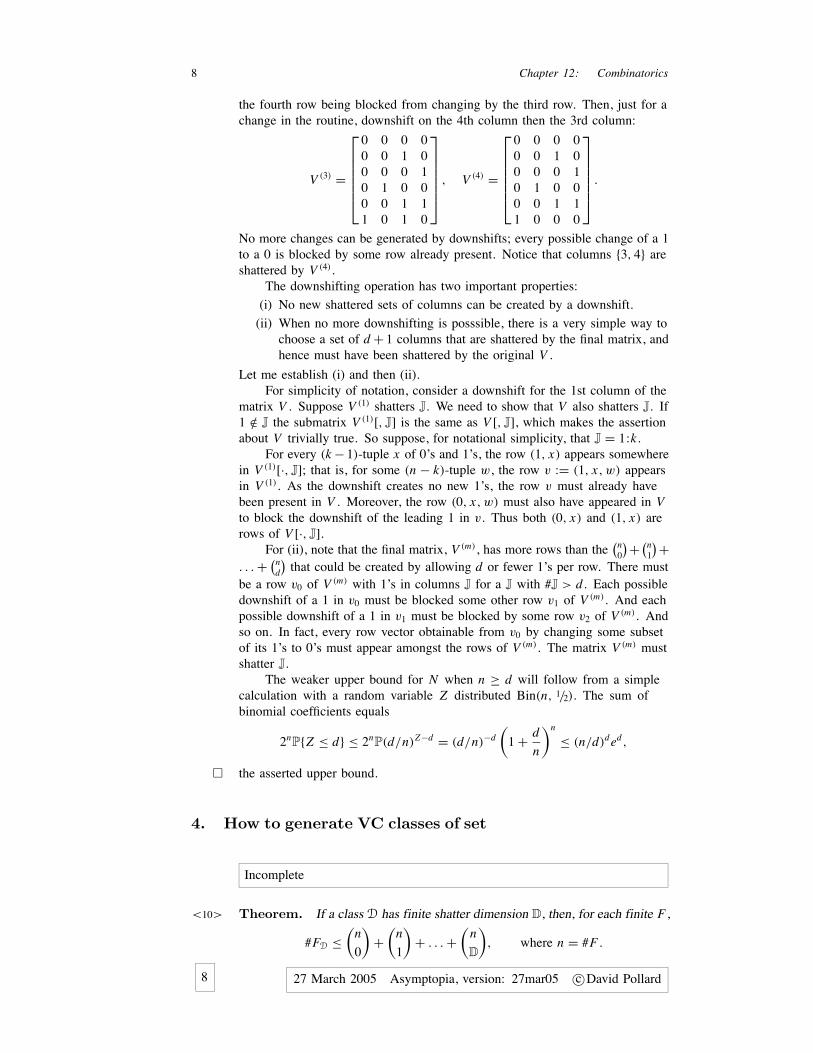
the fourth row being blocked from changing by the third row. Then, just for achange in the routine, downshift on the 4th column then the 3rd column:

V (3) =

⎡⎢⎢⎢⎢⎢⎣

0 0 0 00 0 1 00 0 0 10 1 0 00 0 1 11 0 1 0

⎤⎥⎥⎥⎥⎥⎦ , V (4) =

⎡⎢⎢⎢⎢⎢⎣

0 0 0 00 0 1 00 0 0 10 1 0 00 0 1 11 0 0 0

⎤⎥⎥⎥⎥⎥⎦ .

No more changes can be generated by downshifts; every possible change of a 1to a 0 is blocked by some row already present. Notice that columns {3, 4} areshattered by V (4).

The downshifting operation has two important properties:

(i) No new shattered sets of columns can be created by a downshift.

(ii) When no more downshifting is posssible, there is a very simple way tochoose a set of d + 1 columns that are shattered by the final matrix, andhence must have been shattered by the original V .

Let me establish (i) and then (ii).For simplicity of notation, consider a downshift for the 1st column of the

matrix V . Suppose V (1) shatters J. We need to show that V also shatters J. If1 /∈ J the submatrix V (1)[, J] is the same as V [, J], which makes the assertionabout V trivially true. So suppose, for notational simplicity, that J = 1:k.

For every (k − 1)-tuple x of 0’s and 1’s, the row (1, x) appears somewherein V (1)[·, J]; that is, for some (n − k)-tuple w, the row v := (1, x, w) appearsin V (1). As the downshift creates no new 1’s, the row v must already havebeen present in V . Moreover, the row (0, x, w) must also have appeared in Vto block the downshift of the leading 1 in v. Thus both (0, x) and (1, x) arerows of V [·, J].

For (ii), note that the final matrix, V (m), has more rows than the(n

0

)+ (n1

)+. . . + (n

d

)that could be created by allowing d or fewer 1’s per row. There must

be a row v0 of V (m) with 1’s in columns J for a J with #J > d. Each possibledownshift of a 1 in v0 must be blocked some other row v1 of V (m). And eachpossible downshift of a 1 in v1 must be blocked by some row v2 of V (m). Andso on. In fact, every row vector obtainable from v0 by changing some subsetof its 1’s to 0’s must appear amongst the rows of V (m). The matrix V (m) mustshatter J.

The weaker upper bound for N when n ≥ d will follow from a simplecalculation with a random variable Z distributed Bin(n, 1/2). The sum ofbinomial coefficients equals

2nP{Z ≤ d} ≤ 2n

P(d/n)Z−d = (d/n)−d

(1 + d

n

)n

≤ (n/d)ded ,

the asserted upper bound.�

4. How to generate VC classes of set

Incomplete

<10> Theorem. If a class D has finite shatter dimension D, then, for each finite F ,

#FD ≤(

n

0

)+

(n

1

)+ . . . +

(n

D

), where n = #F .


12.4 How to generate VC classes of set 9

If n ≥ D, the sum of binomial coefficients is bounded above by (en/D)D.

<11> Example. If D is a class of sets with shatter dimension at most D then theclass U = {D1 ∪ D2 : Di ∈ D} has shatter dimension at most 10D. (The boundis crude, but adequate for our purposes.) From a set F of n = 10D points,there are at most (10De/D)D distinct sets F D, with D ∈ D. The trace class FU

consists of at most (10e)n/5 subsets. The class U does not shatter F , because(10e)1/5 < 2.

A similar argument applies to other classes formed from D, such as thepairwise intersections, or complements. The idea can be iterated to generatevery fancy classes with finite shatter dimension (Problem [2]).�

Think of all regions of Rk that can be represented as unions of at mostten million sets of the form { f ≥ 0}, with f a polynomial of degree less thana million, if you want to get some idea of how complicated a class with finiteshatter dimension can be.

Describe cross sections from o-minimal structure.Stengle & Yukich (1989)van den Dries (1998, Chapter 5)

5. Packing numbers for function classes

The connection between shatter dimension and covering numbers introducedin Section 1 extends to more general classes D of measurable subsets of aspace X on which a probability measure P is defined. I will derive an upperbound slightly more precise than before, for the sake of comparison with theresults that will be derived in Section 9. Remember that the packing numberD(ε, D, L1(P)) is defined as the largest number of sets in D separated by atleast ε in L1(P) distance: P(Di�Dj ) > ε for i �= j .

<12> Lemma. Let D be a class of sets with VC-dim(D) ≤ d . Then for eachprobability measure P ,

D(ε, D, L1(P)) ≤(

5

εlog

3e

ε

)d

for 0 < ε ≤ 1.

Remark. If P is concentrated on a finite number of points we neednot worry about measurability.

Proof. Suppose D1, . . . , DN are sets in D with P(Di�Dj ) > ε for i �= j .The asserted bound holds trivially when N ≤ (5 log(3e))d . It is more thanenough to treat the case where log N > d.

Let x = (x1, . . . , xm) be an independent sample of size m = �2(log N )/ε�from P . Notice that 3(log N )/ε > m ≥ d. As in Section 1, for fixed i and j ,

P{Di and Dj pick out same pattern from x} ≤ exp(−mε).

The sum of(N

2

)such probability bounds is strictly less than 1. For some

realization x, the class D picks out N distinct patterns from x, which gives theinequality

N ≤(

m

0

)+

(m

1

)+ . . . +

(m

d

)≤

(em

d

)dbecause m ≥ d.

Tus

N 1/d ≤ 3e log N

dε



From Problem [1], the function g(x) = x/ log x is increasing on the rangee ≤ x < ∞, and if y ≥ g(x) then x ≤ (1 − e−1)−1 y log y. Put x = N 1/d andy = 3e/ε to deduce that

N 1/d ≤ (1 − e−1)−1(3e/ε) log(3e/ε).

The stated bound merely tidies up some constants.�The Lemma has a most useful analog for classes of functions equipped

with various L1(µ) pseudometrics. Let F be a class of real-valued functionson X. Let F be a measurable envelope for F, that is, a measurable functionfor which sup f ∈F | f (x)| ≤ F(x) for every x . Suppose µ is a measure on X

for which µF < ∞. The packing number D(ε, F, L1(µ)) is defined as thelargest N for which there exist functions f1, . . . , fN in F with

µ| fi − f j | > ε for i �= j.

If we replace ε by εµF , the definition becomes invariant to rescalings of µ andthe functions in F. More importantly, in one very common case there will exista bound on the corresponding packing numbers that does not depend on µ, aproperty of great significance in empirical process theory.

<13> Definition. Say that F is a VC-subgraph class if the collection S(F) ofsubgraphs S( f ) := {(x, r) ∈ X ⊗ R : f (x) ≥ r} is a VC class.

<14> Lemma. Let F be a VC-subgraph class with envelope F in L1(µ). Then

D(2εµF, F, L1(µ)) ≤(

5

εlog

3e

ε

)d

for 0 < ε ≤ 1,

if VC-dim(S(F)

) ≤ d .

Proof. Suppose { f1, . . . , fN } ⊆ F with µ| fi − f j | > 2εµF for i �= j . Noticethat each S( fi )�S( f j ) is a subset of

B := {(x, t) ∈ X × R : |t | ≤ F(x)}Let m denote Lebesgue measure on B(R). Write P for the probability measuredefined by P A = µ ⊗ m(AB)/µ ⊗ m(B). By Fubini, µ ⊗ mB = 2µF . Fori �= j it follows that

P(S( fi )�S( f j )

) = µ ⊗ m|{ fi (x) ≥ t} − { f j (x) ≥ t}|2µF

> ε.

Conclude that N ≤ D(ε, S(F), L1(P)), which gives the asserted upper bound.�For many applications it is enough that the covering numbers are uniformly

of order O(ε−W ) for some W .

<15> Definition. A collection of (measurable) functions is said to be Euclideanfor an envelope F if there exist constants A and W for which

D(εµF, F, L1(µ)) ≤ A(1/ε)W for 0 < ε ≤ 1

for every measure µ with F ∈ L1(µ).

In particular, every VC subgraph class is Euclidean, with constants Aand W that depend only on the VC dimension of the set of subgraphs.

For many purposes, an empirical process indexed by a Euclidean class offunctions behaves like a process smoothly indexed by a compact subset of some(finite dimensional) Euclidean space.


12.5 Packing numbers for function classes 11

The existence of packing bounds that work for many different measures µ

allows us to calculate bounds for Lα(µ) packing numbers, for values of α

greater than 1, if F ∈ Lα(µ). For suppose { f1, . . . , fN } ⊆ F with(µ| fi − f j |α

)1/α> ε

(µ(Fα)

)1/αfor i �= j .

Define a new measure λ by dλ/dµ = Fα−1. Then, for i �= j ,

2α−1λ| fi − f j | = µ(2F)α−1| fi − f j |≥ µ(| fi | + | f j |)α−1| fi − f j |≥ µ| fi − f j |α> εαλF

Thus

D(ε(µ(Fα)

)1/α, F, Lα(µ)) ≤ D(εα21−αλ(F), F, L1(λ)) if F ∈ Lα(µ)

≤ Aα(1/ε)Wα if F is Euclidean,

where Aα and Wα are functions of α and of the Euclidean constants, A and W .In particular, if F ∈ L2(µ) then

D(ε(µ(F2)

)1/2, F, L2(µ)) ≤ D

(12ε2λ(F), F, L1(λ)

) ≤ 4A(1/ε)2W .

When specialized to the measure that puts mass 1/n at each of x1, . . . , xn , thelast inequality gives bounds for covering numbers under ordinary Euclideandistance.

6. Fat shattering

The VC-subgraph property of Definition <13> imposes a subtle micro-constraintof the functions in a class F. The property can be destroyed by arbitrarily smallperturbations in the values of the functions, even by perturbations that have anegligible effect on the packing numbers. The concept of fat shattering makesthe shattering property of the functions more robust by requiring a small marginof error for the property that F can shatter a finite set of points.

<16> Definition. Say that a class F of functions ε-surrounds a point x =(x1, . . . , xn) at levels (ξ1, . . . , ξn) if for each subset K of J := {1, . . . , n} thereexists a function fK ∈ F for which

fK(xj )

{ ≥ ξj + ε/2 if j ∈ K

≤ ξj − ε/2 if j ∈ J\K

Define ε-shattering dimension D(F, ε) of F as the largest n for which thereexists an x that is ε-surrounded (at some level) by F.

If F consists of indicator functions of sets, the ε-surround property is thesame for all ε in (0, 1] if ξj ≡ 1/2.

An approximation argument will let us study the consequences of fatshattering as a combinatorial problem. Suppose 0 < ε ≤ 1. Define p := �1/ε�,the largest positive integer for which ε ≤ 1/p. Suppose also that the functionsin F take values in the interval [0, 1]. For each function f in F define v(ε, x, f )

to be the n-tuple of integers with j th element

v(ε, x, f )j := � f (xj )/ε� for j = 1, . . . , n.

That is, v(ε, x, f )j is the unique integer vj in the set Sp := {0, 1, . . . , p} forwhich

f (xj ) = εvj + εj with 0 ≤ εj < ε



Distinct functions f and g might correspond to the same n-tuple. We canidentify the set of all distinct v(ε, x, f ) with the rows of an N ×n matrix Vε,x,F

with elements from Sp. Necessarily, 1 ≤ N ≤ (p + 1)n .If the point x is 2ε-surrounded by F at levels ξ then the integers

kj := �ξj/ε� have the property: for each subset K of J := {1, . . . , n} thereexists a function fK ∈ F for which

<17> v(ε, x, fK)j

{ ≥ kj + 1 if j ∈ K

≤ kj − 1 if j ∈ J\K.

Conversely, if <17> holds then

fK(xj ) = εv(ε, x, fK)j + εj

{ ≥ εkj + ε if j ∈ K

≤ εkj − (ε − εj ) < εkj if j ∈ J\K,

which implies that x is ε/2-surrounded by F at levels ε(kj + 12 ).

In reducing the possibly infinite set of functions F to the finite matrix Vε,x,F

we sacrifice only a factor of 2 is our study of fat shattering.

<18> Definition. Let Ln := ∪JZJ, the union running over all nonempty subsets

of {1, . . . , n}, and say that a lattice point ζ ∈ ZJ has degree #J.Write M(n, p) for the set of all matrices with n columns and distinct rows

with elements from Sp := 0: p. Let J be a nonempty subset of {1, . . . , n}. Saythat a lattice point ζ ∈ ZJ is 2-surrounded by a V in M(n, p) if for each ofthe 2#J subsets K of J there is a row iK of V for which

V [iK, j]

{ ≥ ζj + 1 if j ∈ K

≤ ζj − 1 if j ∈ J\K.

Define the 2-shatter dimension D2(V ) to be the largest degree of a lattice point2-surrounded by V . Define the 2-surround number S2(V ) as the number ofdistinct lattice points from Ln that are 2-surrounded by V .

FALSE: The set M1 is the set of binary matrices. The definitions for p = 1are just slight reformulation of properties of binary matrices.

For a given J with #J = k and ζ ∈ ZJ, there are at most p − 1choices for each ζj if the lattice point is to be surrounded. There are at most(n

k

)(p − 1)k lattice points of degree k that could possibly be 2-surrounded by a

matrix V ∈ M(n, p). If

S2(V ) >∑d

k=1

(n

k

)(p − 1)k,

the pigeon-hole principle shows that there must be at least one lattice point ofdegree at least (d + 1) that is 2-surrounded by V ; and if D2(V ) ≤ d then

S2(V ) ≤∑d

k=1

(n

k

)(p − 1)k .

In particular, if x is 2ε-surrounded by F then D2(Vε,x,F

) ≥ dhas 2-shatter dimension d For a matrix????

7. Mendelson and Vershynin

Based on Mendelson & Vershynin (2003).


12.7 Mendelson and Vershynin 13

<19> Theorem. Suppose V is an N × n matrix in Mp. For α ∈ [1, ∞) define

Kα := ( ∑k≥2 kα2−k

)1/αand Cα := 2(1+α)/α3Kα . Suppose the rows of V are

Cα-separated, in the sense that(n−1

∑j≤n

|V [i1, j] − V [i2, j]|α)1/α

≥ Cα for all 1 ≤ i1 < i2 ≤ n.

Then(i) S2(V ) ≥ √

N − 1.(ii) if D2(V ) ≤ d then

√N ≤ ∑d

k=0

(nk

)pk ≤ (epn/d)d .

<20> Lemma. Let X be a random variable with zero median for which ∞ >

P|X |α ≥ τα . Then there exists a β ∈ (0, 1/2] and an interval [a, b] of lengthat least τ/Kα such that either

P{X ≤ a} ≥ β/2 and P{X ≥ b} ≥ 1 − β

or

P{X ≤ a} ≥ 1 − β and P{X ≥ b} ≥ β/2

Proof. Represent X as q(U ) where q is an increasing function with q(1/2) = 0and U has a Uniform(0, 1) distribution. With no loss of generality, supposeσα := 2P|q(U )|α{U > 1/2} ≥ τα . Suppose a constant c has the property that

<21> q(1 − β) + cσ > q(1 − β/2) for 0 < β ≤ 1/2.

Repeated appeals to this inequality for β = 2−k for k = 1, 2, . . . followed by atelescoping summation give kcσ > q

(1 − 2−k−1

), and hence

σα = 2∑∞

k=1

∫ 1−2−k−1

1−2−k

q(u)αdu ≤∑∞

k=12−kq

(1 − 2−k−1

)α<

(cσ Kα

)α.

Inequality <21> must therefore fail if we choose c = 1/Kα: there must existsome β in (0, 1/2] for which q(1 − β) + σ/Kα ≤ q(1 − β/2). For that β wehave

P{X ≥ q(1 − β/2)} ≥ P{U ≥ 1 − β/2} = β/2

P{X ≤ q(1 − β)} ≥ P{U ≤ 1 − β} = 1 − β.

Analogous inequalities hold if we shrink the interval to have length τ/Kα .�<22> Corollary. For the matrix V from Theorem <19> there exists a constant

β ∈ (0, 1/2], a column j0, and an integer η such that both subsets

<23> I1 := {i : V [i, j0] ≥ η + 1} and I2 := {i : V [i, j0] ≤ η − 1}are nonempty, with

max(#I1, #I2

) ≥ (1 − β)N and min(#I1, #I2

) ≥ βN/2.

Proof. Independently select I1 and I2 from the uniform distributionon {1, 2, . . . , N }. We have P{I1 = I2} = 1/N . When I1 �= I2 the corre-sponding rows of V are Cα separated. Thus

P∑

j≤n|V [I1, j] − V [I2, j]|α ≥ nCα

α

(1 − N−1

) ≥ 12 nCα

α ,

which implies existence of at least one j0 for which

P|V [I1, j0] − V [I2, j0]|α ≥ 12 Cα

α .

Let m0 be a median for the distribution of the random variable V [I1, j0]. Viathe inequality |x + y|α ≤ 2α−1

(|x |α + |y|α)for real numbers x and y deduce

that2α

P|V [I1, j0] − m0|α ≥ 12 Cα

α



The random variable X := V [I1, j0] − m0 has P|X |α ≥ 12 (Cα/2)α = (3Kα)α . A

gap of length 3Kα/Kα must contain at least one interval (η − 1, η + 1) with η

an integer.�Proof of Theorem <19>. Assertion (ii) follows from assertion (i), as explainedin the previous Section.

Assertion (i) is trivial for N = 1. For the purposes of an inductive proof,suppose that N ≥ 2 and that the assertion is true for matrices with smallernumbers of rows.

For simplicity of notation, suppose the j0 from Corollary <22> equals 1.Write Nr for #Ir and Vr for V [Ir , ], for r = 1, 2.

Consider a J with 1 ∈ J. If V1 2-surrounds a lattice point ζ ∈ ZJ we musthave ζ1 ≥ η + 1; and if V2 2-surrounds ζ we must have ζ1 ≤ η − 1. It istherefore impossible for both V1 and V2 to 2-surround the same lattice point inthis ZJ. In particular, neither Vr can 2-surround η in its role as a lattice pointfrom Z{1}.

Define

L(1) := {ζ ∈ L : only V1 2-surrounds ζ }

L(2) := {ζ ∈ L : only V2 2-surrounds ζ }

L(1,2) := {ζ ∈ L : both V1 and V2 2-surround ζ }

Clearly V surrounds every point in L(1) ∪ L(2) ∪ L(1,2). If ζ ∈ LJ ∩ L(1,2)

we must have 1 /∈ J. Neither Vr can surround the lattice point (η, ζ ) ∈ L{1}∪J

but V does: the submatrix V1 provides all those iK for which V [iK, 1] > η

and the submatrix V2 provides all those iK for which V [iK, 1] < η. In short,for each ζ 2-surrounded by both V1 and V2 there are two centers, ζ ∈ L(1,2)

and (η, ζ ) /∈ S(V1) ∪ S(V2), 2-surrounded by V . It follows that

<24> S2(V ) ≥ 1 + #L(1) + #L

(2) + 2 × #L(1,2) = 1 + S2(V1) + S2(V2).

Invoke the inductive hypothesis for both submatrices V1 and V2 to conclude that

S2(V ) ≥ 1+ (√

N 1 −1)+ (√

N 2 −1) =√

N(√

β/2 +√

1 − β)−1 ≥

√N −1.

Assertion (i) follows by induction on N .�

8. Haussler and Long

Based on Haussler & Long (1995)Define

ψ(i, j) ={ 1 if i = j

0 if i < j if i > j

For u, v ∈ Zk define

ψ(u, v) = (ψ(u1, v1), . . . , ψ(uk, vk)

) ∈ {0, 1, }k

Let V be an N × n matrix in M(n, p). For a nonempty subset J of{1, . . . , n} say that V ψ-shatters J if there exists a ζ ∈ ZJ such that

{ψ (V [i, J], ζ

): 1 ≤ i ≤ N } ⊇ {0, 1}J.

That is, for each subset K of J there exists an iK such that

<25> ψ(V [iK, j], ζj

) ={

1 if j ∈ K

0 if j ∈ J\K


12.8 Haussler and Long 15

Write Dψ(V ) for the largest d for which some set J of d columns of V isψ-shattered.

For 0 ≤ d ≤ n and n ≥ 1 define �(n, d, p) as the smallest integer forwhich: if V is an N × n matrix in M(n, p) for which N > �(n, d, p) thenthere is some subset J of at least d +1 columns that is ψ-shattered by V . Show

<26> �(n, d, p) ={

1 for d = 0(1 + p)n for d = n

for n = 1, 2, . . .

The second equality corresponds to the fact that no matrix in M(n, p) has morethan (1 + p)n rows.

<27> Theorem. For 0 ≤ d ≤ n,

�(n, d, p) =d∑

k=0

(n

k

)pk

Proof. Notice that the asserted value for �(n, d, p) is exactly equal to

G(n, d, p) := #{x ∈ Snp : x has at most d nonzero entries}

By counting separately for those x that end with a zero and those that end withone of the p integers 1, . . . , p, we get a recursive expression for G,

<28> G(n + 1, d, p) = G(n, d, p) + pG(n, d − 1, p),

which together with the equality

G(1, d, p) ={

1 for d = 01 + p for d = 1

uniquely determines G.Argue by induction on n. True for n = 1. Suppose true for values up to

n, for some n ≥ 1. Prove it for n + 1.Suppose V ∈ M(n + 1, p). For each i , call V [i, 1:n] the prefix of the row

and V [i, n + 1] the suffix. Write W for set of all distinct prefixes in V . Foreach w ∈ W, write Vw for the submatrix consisting of all rows with prefix w.Write kw for the smallest suffix amongst the rows in Vw. All other rows in Vw

have suffix strictly greater than kw.Suppose #W = N0. Let I0 denote the set of N0 rows of the form (w, kw)

for w ∈ W. The suffix for every remaining row must be at least 1. Write Is

for the set of rows in (1 : N )\I0 with suffix s, for s = 1, 2, . . . , p. Note thatN = ∑p

s=0 Ns . Now suppose that

N > �(n, d, p) + p�(n, d − 1, p) for some d with 1 ≤ d ≤ n.

Then either

(i) N0 > �(n, d, p)

or

(ii) Ns > �(n, d − 1, p) for some s ≥ 1In the first case, the N0 × (n + 1) matrix V [I0, ], which has distinct

rows, must shatter some set of d + 1 columns, by the inductive hypothesis. Inthe second case, the Ns × n matrix V [Is, 1 : n], which also has distinct rows(otherwise two rows of V with suffix s would have the same prefix), mustshatter some set J of d columns from 1:n. That is, there exists some ζ ∈ ZJ

such that for each subset K of J there exists an iK ∈ Is with

ψ(V [iK, j], ζj

) ={

1 if j ∈ K

0 if j ∈ J\K.



Let i ′K

∈ I0 be such that V [iK, ] and V [i ′K, ] have the same prefix. Define

ξ := (ζ, s). Then V shatters J := J ∪ {n + 1}:

ψ(V [iK, j], ξj

) ={

1 if j ∈ K

0 if j ∈ J\Kwhere K := K ∪ {n + 1}

and

ψ(V [i ′

K, j], ξj

) ={

1 if j ∈ K

0 if j ∈ J\K.

In either case, we have a set of d + 1 columns shattered by V .It follows that

<29> �(n + 1, d, p) ≤ �(n, d, p) + p�(n, d − 1, p).

Together with <26>, this inequality determines an upper bound for �(n, d, p).Indeed, if we define �(n, d, p) = G(n, d, p)−�(n, d, p) then <30> and <28>

give the recursive inequality

<30> �(n + 1, d, p) ≥ �(n, d, p) + p�(n, d − 1, p)

with the initial condition �(1, d, p) = 0 for d = 0, 1. It follows that�(n, d, p) ≤ G(n, d, p).

In fact, the last inequality must be an equality, because the G(n, d, p) × nmatrix V consisting of all rows from Sn

p with at most d nonzero elementscannot shatter any set J of more than d columns: to get <25> with K = ∅ wewould need ζj > 0 for all j in J; but then at most d elements of ψ

(V [i, J], ζ

)could equal 1.�

9. An improvement of the packing bound

By means of a more subtle randomization argument, it is possible to eliminatethe log(6e/ε) factor from the bound in Theorem <14>, with a change in theconstant. The improvement is due to Haussler (1995).

<31> Theorem. Let V be an N × n binary matrix for which∑j≤n

{V [i1, j] �= V [i2, j]} ≥ nε for all 1 ≤ i1 < i2 ≤ n.

for some 0 < ε ≤ 1. ThenNot what Haussler got.

N ≤ e(1 + VC-dim) (2e/ε)D

where D = D(V ), the shatter dimension of V .

For Haussler’s method, we generate random variables X j := V [I, j]and random vectors XK := V [I, K] by means of an I that is uniformlydistributed on 1: N . The separation assumption of the Theorem provides (viaLemma <32>) a lower bound for∑

#K=m

∑j /∈K

Pvar(X j | XK),

where the first sum runs over all subsets K of size m − 1 from 1 : n, fora strategically chosen value of m. An elegant extension of Theorem <8>

provides (via Lemma <35>) an upper bound for the same quantity. The pairof bounds gives an inequality involving N , n, ε and D, which leads to theinequality asserted by the Theorem.

Remark. My m corresponds to m − 1 in Haussler’s paper.

To keep the notation simple, I will prove unconditional forms of thetwo Lemmas, then deduce the conditional forms by applying the Lemmas tosubmatrices of V .


12.9 An improvement of the packing bound 17

<32> Lemma. Let I be uniformly distributed on 1:N ,∑j≤n

var(X j ) ≥ 12 nε

(1 − N−1

).

Proof. Let I ′ be chosen independently of I , with the same uniform distribution.Write X ′

j for V [I ′, j]. Note that the difference X j − X ′j takes the values ±1

when V [I, j] �= V [I ′, j] and is otherwise zero. Then∑jvar(X j ) =

∑j

12 P|X j − X ′

j |2 by independence

= 12 P

∑j{V [I, j] �= V [I ′, j]}.

Whenever I �= I ′ which happens with probability 1 − N−1, the last sum isgreater than nε.�

For the second Lemma we need another inequality involving the shatterdimension. Write Ej for the set of all pairs (i1, i2) for which the two rowsV [i1, ] and V [i2, ] differ only in the j th position. Define E = ∪j≤nEj . Call thepairs in E edges: If we were to identify each row of V with a vertex of thehypercube {0, 1}n , then E would correspond to a set of edges between pairs ofoccupied vertices a distance 1 apart.

By means of a slight modification of the downshifting argument fromTheorem <8>, Problem [5] shows that

<33> #E ≤ ND.

Using the analogous property for subsets of E, Problem [6], then shows that itis possible to provide an orientation for each edge, so that edge e points fromvertex ie

1 to vertex ie2 , in such a way that no vertex has in-degree greater than D:

<34> #{e : ie2 = i} ≤ D for 1 ≤ i ≤ N .

When we apply the Lemma to submatrices of V the distribution of I willnot be uniform. We will need the Lemma for more general distributions.

<35> Lemma. For X j := V [I, j] and X− j := V [I, − j],∑n

j=1Pvar

(X j | X− j

) ≤ D.

under every distribution P for I .

Proof. The random vector X− j takes values in V− j , the set of distinct rowsof V [, − j]. For each v ∈ V− j , the set {i : V [i, − j] = v} contains either oneor two values: either v uniquely determines the i for which V [i, − j] = v, orthere is an edge e = (ie

1 , ie2) in Ej for which V [ie

1 , − j] = V [ie2 , − j] = v. There

is a partition of V− j into two subsets, V1− j and V2

− j , corresponding to these twopossibilities. There is a one-to-one correspondence between Ej and pairs ofrows from V2

− j ; and if v ∈ V2j corresponds to the edge e then P{X− j = v} = Pe.

Once we know X− j = v, the value of I is either uniquely determined(if v ∈ V1

− j ) or is one of the two vertices of an edge e in Ej with conditionalprobabilities P{ie

1}/Pe and P{ie2}/Pe. Thus

var(X j | X− j = v) ={

0 if v ∈ V1j

P{ie1}P{ie

2}/(Pe)2 if v ∈ V2j .

Averaging over the choice of edge corresponding to v we getn∑

j=1

Pvar(X j | X− j ) =n∑

j=1

∑e∈Ej

Pe(P{ie

1}P{ie2}/(Pe)2

) ≤∑e∈E

P{ie2}.

As e ranges over all edges, ie2 visits each vertex at most D times. The last sum

is at most D∑

i≤N P{i} = D.�



Proof of Theorem <31>. Let J be a subset of 1:n. The uniform distributionon 1:N induces a distribution P on VJ, with Pv = Nv/N if v appears Nv timesas a row of V [, J]. A submatrix of V [, J] with only one copy of each v fromVJ cannot have a shatter dimension larger than D(V ). Applying Lemma <35>

to that matrix we get ∑j∈J

Pvar(X j | XJ\{ j}

) ≤ D.

Remark. You should not be worried by the fact that the rows of thenew matrix might not be ε-separated. In fact, the proof of the Lemma madeno use of the separation assumption. It would have been more precise tostate the Lemma as an assertion about binary matrices with a given shatterdimension.

Sum the last inequality over all possible subsets J of 1:n with #J = m + 1,for a value of m that will be specified soon.∑

#J=m+1

∑j∈J

Pvar(X j | XJ\{ j}) ≤(

n

m + 1

)D.

Write K for J\{ j}. Every ( j, K) pair with j /∈ K and #K = m appears exactlyonce in the double sum. The inequality is equivalent to

<36>∑

#K=m

∑j /∈K

Pvar(X j | XK) ≤(

n

m + 1

)D.

As a check, note that the double sums involve (m + 1)( n

m+1

) = (n − m)(n

m

)terms.

For a fixed K and a fixed v in VK, the distribution of I conditionalon X K = v is uniform over the rows of the N (v, K) × (n − m) submatrix Vv,K

of V [, −K] consisting of those rows for which V [i, K] = v. Moreover,∑j /∈K

|V [i1, j] − V [i2, j]| =∑

j≤n|V [i1, j] − V [i2, j]| ≥ nε

for rows i1 < i2 of Vv,K. Apply Lemma <32> to that submatrix.∑j /∈K

var(X j |XK = v) ≥ 12 nε

(1 − N (v, K)−1

).

Remark. The proof of Lemma <32> is valid when N (v, K) = 1, eventhough the ε-separation property is void for a matrix with only one row. Inany case, the lower bound becomes zero when N (v, K) = 1.

Average over the possible values for XK, using the fact that P{XK = v} =N (v, K)/N for each v in VK.

<37>∑j /∈K

Pvar(X j |XK) ≥ 12 nε

∑v∈VK

(N (v, K)/N − N−1

) = 12 nε

(1 − #VK/N

)From Theorem <8>,

#VK ≤ p(m, D) :=(

m

0

)+ . . . +

(m

D

)≤ (em/D)D if m ≥ D.

Sum over all(n

m

)subsets K of size m to get the companion lower bound

to <36>. (n

m

)12 nε

(1 − p(m, D)/N

) ≤∑

#K=m

∑j /∈K

Pvar(X j | XK)

Together the two bounds imply(n

m

)12 nε

(1 − p(m, D)

N

)≤

(n

m + 1

)D,


12.9 An improvement of the packing bound 19

which rearranges to

N ≤ p(m, D)

/(1 − 2(n − m)

nε(m + 1)D

).

We could try to optimize over m immediately, as Haussler did, to bound Nby a function of ε, D, and n, then take a supremum over n. However, it issimpler to note that all the conditions of the Theorem apply to the N × �nmatrix obtained by binding together � copies of V . Thus the last inequalityalso holds if we replace n by �n, for an arbitrarily large �. Letting � tend toinfinity with m fixed, we then eliminate n from the bound.

N ≤ p(m, D)

/(1 − 2D

ε(m + 1)

)If we choose m = �2(D + 1)/ε� then m ≥ D and the upper bound for N issmaller than(em

D

)D ε(m + 1)

ε(m + 1) − 2D≤ (2e/ε)D

(1 + D

−1)D 2D + 2

2D + 2 − 2D,

which is smaller than the bound stated in the Theorem.

10. Problems

[1] Define g(x) = x/(log x) for x > 1.

(i) Show that g achieves its minimum value of e at x = e and that g is anincreasing function on [e, ∞).

(ii) Suppose y ≥ g(x) for some x ≥ e. Show that log y ≥ (1 − e−1) log x .Deduce that x ≤ (1 − e−1)−1 y log y.

[2] Let D1, . . . ,Dk be classes of sets each with VC dimension at most VC-dim.Let Bk denote the class of all sets expressible by means of at most k union,intersection, or complement symbols. Find an increasing, integer-valuedfunction β(k) such that the VC dimension of Bk is at most β(k)VC-dim.

[3] (generalized marriage lemma) Let S and T be finite sets and R be a nonemptysubset of S × T . Let µ be a finite, nonnegative measure on S and ν be a finite,nonnegative measure on T . Say that a nonnegative measure λ on S × T is asolution to the (µ, ν, R, S, T ) problem if

(a) λRc = 0

(b) λ({i} × T

) ≤ µ{i} for all i ∈ S

(c) λ(S × { j}) ≤ ν{ j} for all j ∈ T .

Write Rj for {i ∈ T : (i, j) ∈ R} and RJ for ∪j∈J Rj for subsets J of S. By thefollowing steps, show that there exists a solution for which all the inequalitiesin (c) are actually equalities if and only if

(∗) ν(J) ≤ µ(RJ

)for all J ⊆ T .

(i) If λ is a solution with equalities in (c) for every j , then

ν(J) = λ(S × J) = λ(RJ × J

) ≤ µ(RJ) for each J ⊆ T .

(ii) Now suppose (∗) holds. Let λ be a maximal solution to the (µ, ν, R, S, T )

problem, that is, a solution for which λR is as large as possible. Showthat there cannot exist an (i, j) in R for which λ

({i} × T)

< µ{i} andλ

(S × { j}) < ν{ j}, for otherwise λR could be increased by adding some

more mass at (i, j).



(iii) Deduce that there must exist at least one j for which equality holds in (c),for otherwise µRT = ∑

i λ({i} × T

) = λR < νT , contradicting (∗).

(iv) Without loss of generality, suppose λ(S × {1}) = ν{1}. Define R :=

R\ (T × {1}). Let λ be the restriction of λ to R and ν be the restriction

of ν to S\{1}. Define λ1 to be the measure on S for which λ1{i} =λ{(i, 1)}. Define µ = µ − λ1. Show that λ is a maximal solution to the(µ, ν, R, S\{1}, T ) problem. Hint: If there were another solution γ withγ (R) > λ(R), then the measure obtained by pasting together γ and λ1

would give a solution to the original problem with total mass strictlygreater than λR.

(v) Repeat the argument from (iv), but starting from λ as a maximal solutionto the (µ, ν, R, S\{1}, T ) problem, to deduce equality in (c) for anothercolumn. And so on.

[4] Show that assertion of Problem [3] is still valid if the measures λ, µ, and ν areretricted to take nonnegative integer values.

[5] Suppose an N × n binary matrix V has shatter dimension VC-dim. Let E bethe corresponding edge set, as defined in Section 9. Show that #E ≤ NVC-dimby following these steps.

First show that the downshift operation used for the proof of Theorem <8>

cannot decrease the number of edges. Suppose V is transformed to V ∗ by adownshift of the first column. Suppose (i1, i2) is an edge of V but not of V ∗.

(i) Suppose V [i1, ] and V [i2, ] differ only in the j th position. Show thatj > 1, for otherwise V ∗[i1, ] and V ∗[i2, ] would differ only in the firstposition.

(ii) Show that V [i1, 1] = V [i2, 1] = 1, for otherwise the downshift could notchange either row.

(iii) Suppose V [i1, ] = (1, w) and V ∗[i1, ] = (0, w) and V [i2, ] = V ∗[i2, ] =(1, y), where w and y differ only in the j th position. Show that (0, y) =V [i0, ] = V ∗[i0, ] for some i0.

(iv) Deduce that (i0, i1) is an edge of V ∗ but not an edge of V .

(v) Explain why every downshift that destroys an edge creates a new one.

Now suppose that V ∗ is the result of not just one downshift, but that it is thematrix that remains when no more downshifting is possible. Let E∗ be its setof edges.

(vi) Explain why #E∗ ≥ #E.

(vii) Argue as in the proof of Theorem <8> to show that no row of V ∗ cancontain more than D ones.

(viii) Define ψ : E∗ → 1 : N by taking ψ(e) as the row corresponding to thevertex of e with the larger number of ones. Show that ψ−1(i) contains atmost D edges, for every i . Hint: How many different edges can be createdby discarding a 1 from V ∗[i, ]?

(ix) Deduce that #E∗ ≤ ND.

[6] Suppose V be an N ×n binary matrix with shatter dimension D and edge set E.Show that there exists a map ψ : E → 1:N such that

(a) ψ(e) is one of the two vertices on the edge e,

(b) #ψ−1(i) ≤ VC-dim for every i ,

by following these steps.


12.10 Problems 21

(i) Let E0 be a subset of E, with vertices all contained in I ⊆ 1:N . Apply theresult from Problem [5] to show that

#E0 ≤ number of edges of V [I, ] ≤ D #I.

(ii) Invoke the result from Problem [4] with

S = 1:N T = E Re = the pair of vertices of e

and ν{e} = 1 for each e and µ{i} = D for each i . Show that the measureλ puts a single atom of mass 1 in each Re.

(iii) Let ψ(e) be the vertex in Re where λ puts its mass. Show that

#ψ−1(i) = λ({i} × E

) ≤ µ{i} ≤ D.

11. Notes

Get the history on VC Lemma straight. VC? Sauer (1972) ? Frankl?Section 3: Dudley for sets; Pollard (1982) via Le Cam for functions.Section 4: Haussler. Explain why result is interesting.Downshift technique: compare with original VC argument. Talagrand?

Haussler, and refs. Compare with Ledoux & Talagrand (1991, p. 420) anddifferent explanation in Talagrand (1987). Check the 1987 survey article ofFrankl, cited by Haussler.

Cover (1965) for exact bound for half-spaces. More comments onsuboptimality of VC bound? What does the cubic vs quadratic say aboutattempts to squeeze the best results from the VC bound?

Vapnik & Cervonenkis (1971) Cite other VC paper too.Steele (1975) Cite Steele paper, and Sauer, and Frankl.Talagrand (2003)

References

Cover, T. M. (1965), ‘Geometric and statistical properties of systems of linearinequalities with applications to pattern recognition’, IEEE Transactionson Elec. Comp.

Dudley, R. M. (1978), ‘Central limit theorems for empirical measures’, Annalsof Probability 6, 899–929.

Haussler, D. (1995), ‘Sphere packing numbers for subsets of the Boolean n-cubewith bounded Vapnik-Chervonenkis dimension’, Journal of CombinatorialTheory 69, 217–232.

Haussler, D. & Long, P. M. (1995), ‘A generalization of Sauer’s lemma’,Journal of Combinatorial Theory 71, 219–240.

Ledoux, M. & Talagrand, M. (1991), Probability in Banach Spaces: Isoperime-try and Processes, Springer, New York.

Mendelson, S. & Vershynin, R. (2003), ‘Entropy and the combinatorialdimension’, Inventiones mathematicae 152, 37–55.

Pollard, D. (1982), ‘A central limit theorem for k-means clustering’, Annals ofProbability 10, 919–926.

Sauer, N. (1972), ‘On the density of families of sets’, Journal of CombinatorialTheory 13, 145–147.

Steele, J. M. (1975), Combinatorial Entropy and Uniform Limit Laws, PhDthesis, Stanford University.

Stengle, G. & Yukich, J. (1989), ‘Some new Vapnik-Chervonenkis classes’,Annals of Statistics 17, 1441–1446.



Talagrand, M. (1987), ‘Donsker classes and random geometry’, Annals ofProbability 15, 1327–1338.

Talagrand, M. (2003), ‘Vapnik-Chervonenkis type conditions and uniformDonsker classes of functions’, Annals of Probability 31, 1565–1582.

van den Dries, L. (1998), Tame Topology and O-minimal Structures, CambridgeUniversity Press.

Vapnik, V. N. & Cervonenkis, A. Y. (1971), ‘On the uniform convergence ofrelative frequencies of events to their probabilities’, Theory Probabilityand Its Applications 16, 264–280.


Documents

Chapter 12 Combinatorics - Yale University · Chapter 12 Combinatorics ... SECTION 5 establishes a connection between VC dimension and packing ... can also be applied to collections