Chapter 14: Query Optimization - Yale Universitycodex.cs.yale.edu/avi/db-book/db5/slide-dir/ch14.pdf · Database System Concepts - 5th Edition, Oct 5, 2006. 14.2 ©Silberschatz, Korth

Database System Concepts 5th Ed.©Silberschatz, Korth and Sudarshan

See www.db-book.com for conditions on re-use

Chapter 14: Query OptimizationChapter 14: Query Optimization

©Silberschatz, Korth and Sudarshan14.2Database System Concepts - 5th Edition, Oct 5, 2006.

Chapter 14: Query OptimizationChapter 14: Query Optimization

Introduction Transformation of Relational ExpressionsCatalog Information for Cost EstimationStatistical Information for Cost EstimationCost-based optimizationDynamic Programming for Choosing Evaluation PlansMaterialized views


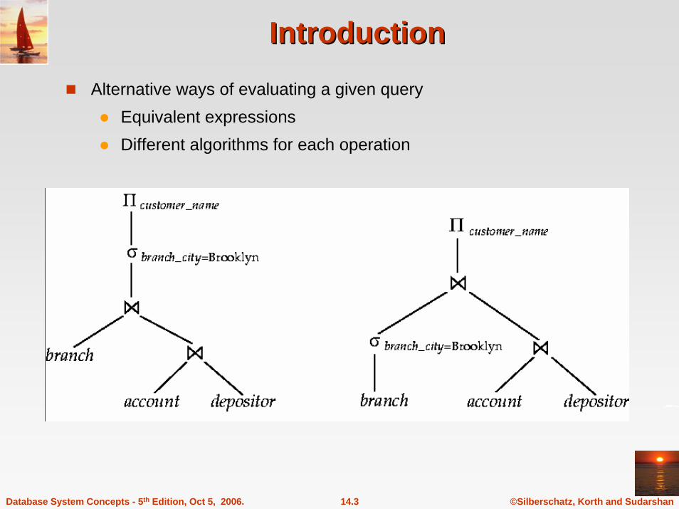
IntroductionIntroductionAlternative ways of evaluating a given query

Equivalent expressionsDifferent algorithms for each operation


Introduction (Cont.)Introduction (Cont.)

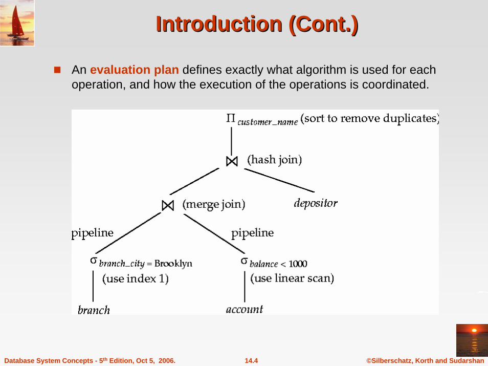
An evaluation plan defines exactly what algorithm is used for each operation, and how the execution of the operations is coordinated.


Introduction (Cont.)Introduction (Cont.)

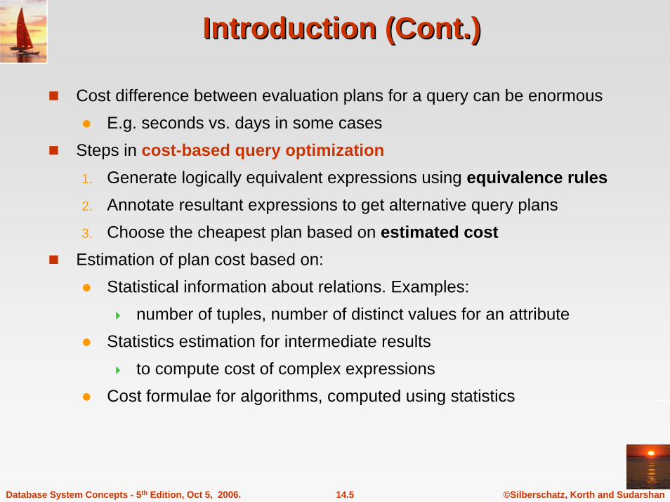
Cost difference between evaluation plans for a query can be enormousE.g. seconds vs. days in some cases

Steps in cost-based query optimization1. Generate logically equivalent expressions using equivalence rules2. Annotate resultant expressions to get alternative query plans3. Choose the cheapest plan based on estimated cost

Estimation of plan cost based on:Statistical information about relations. Examples:

number of tuples, number of distinct values for an attributeStatistics estimation for intermediate results

to compute cost of complex expressionsCost formulae for algorithms, computed using statistics



Generating Equivalent ExpressionsGenerating Equivalent Expressions


Transformation of Relational ExpressionsTransformation of Relational Expressions

Two relational algebra expressions are said to be equivalent if the two expressions generate the same set of tuples on every legal database instance

Note: order of tuples is irrelevantIn SQL, inputs and outputs are multisets of tuples

Two expressions in the multiset version of the relational algebra are said to be equivalent if the two expressions generate the same multiset of tuples on every legal database instance.

An equivalence rule says that expressions of two forms are equivalent

Can replace expression of first form by second, or vice versa


Equivalence RulesEquivalence Rules

1. Conjunctive selection operations can be deconstructed into a sequence of individual selections.

2. Selection operations are commutative.

3. Only the last in a sequence of projection operations is needed, the others can be omitted.

4. Selections can be combined with Cartesian products and theta joins.a. σθ(E1 X E2) = E1 θ E2

b. σθ1(E1 θ2 E2) = E1 θ1∧ θ2 E2

))(())((1221

EE θθθθ σσσσ =

))(()(2121

EE θθθθ σσσ =∧

)())))((((121

EE LLnLL Π=ΠΠΠ KK


Equivalence Rules (Cont.)Equivalence Rules (Cont.)

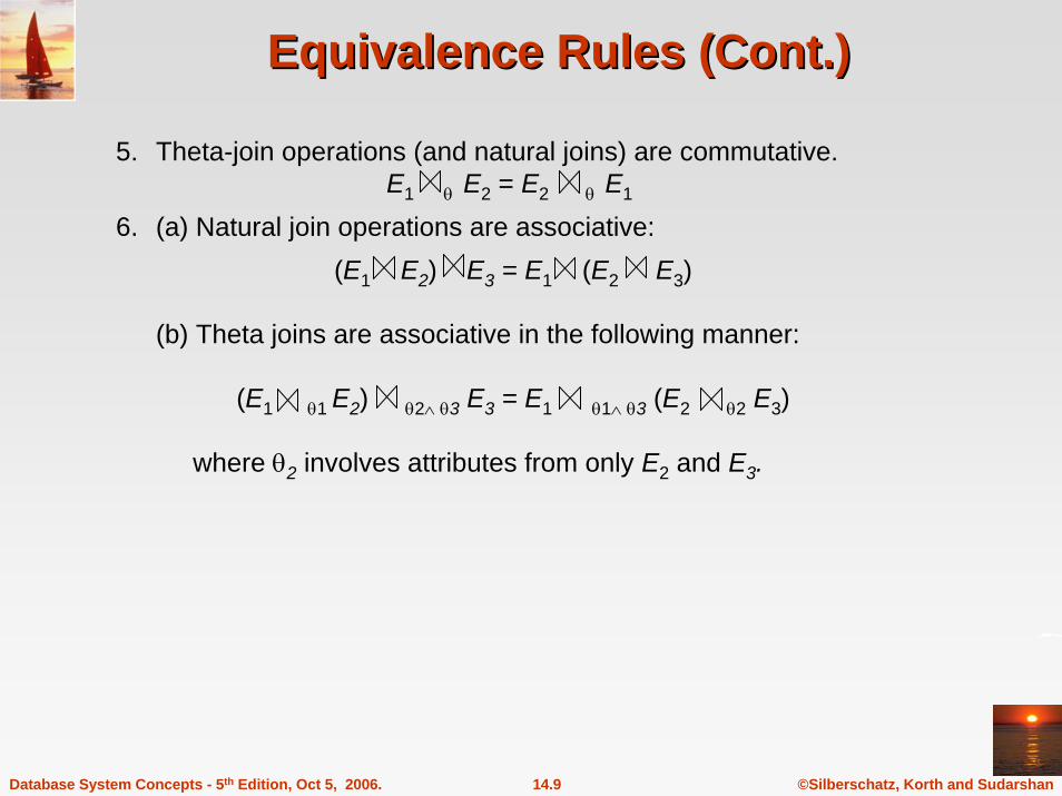
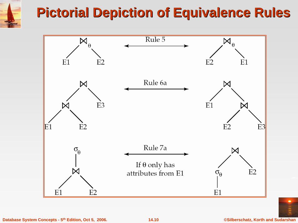
5. Theta-join operations (and natural joins) are commutative.E1 θ E2 = E2 θ E1

6. (a) Natural join operations are associative:(E1 E2) E3 = E1 (E2 E3)

(b) Theta joins are associative in the following manner:

(E1 θ1 E2) θ2∧ θ3 E3 = E1 θ1∧ θ3 (E2 θ2 E3)

where θ2 involves attributes from only E2 and E3.


Pictorial Depiction of Equivalence RulesPictorial Depiction of Equivalence Rules



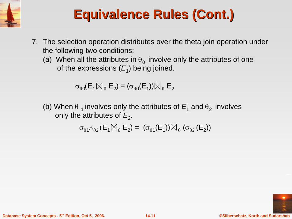
7. The selection operation distributes over the theta join operation under the following two conditions:(a) When all the attributes in θ0 involve only the attributes of one

of the expressions (E1) being joined.

σθ0(E1 θ E2) = (σθ0(E1)) θ E2

(b) When θ 1 involves only the attributes of E1 and θ2 involves only the attributes of E2.

σθ1∧θ2 (E1 θ E2) = (σθ1(E1)) θ (σθ2 (E2))



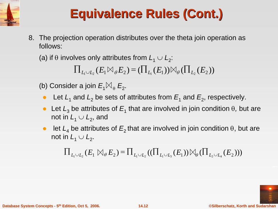
8. The projection operation distributes over the theta join operation as follows:(a) if θ involves only attributes from L1 ∪ L2:

(b) Consider a join E1 θ E2. Let L1 and L2 be sets of attributes from E1 and E2, respectively. Let L3 be attributes of E1 that are involved in join condition θ, but are not in L1 ∪ L2, andlet L4 be attributes of E2 that are involved in join condition θ, but are not in L1 ∪ L2.

))(())(()( 2121 2121 EEEE LLLL ∏∏=∏ ∪ θθ

)))(())((()( 2121 42312121EEEE LLLLLLLL ∪∪∪∪ ∏∏∏=∏ θθ



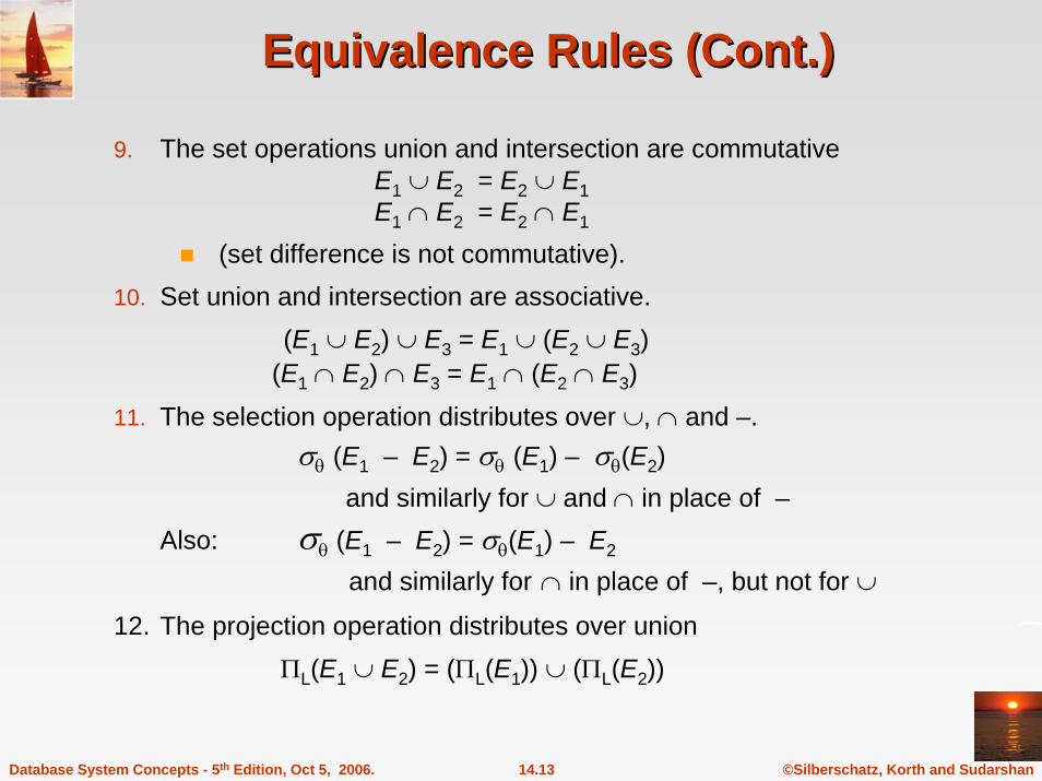
9. The set operations union and intersection are commutative E1 ∪ E2 = E2 ∪ E1E1 ∩ E2 = E2 ∩ E1

(set difference is not commutative).10. Set union and intersection are associative.

(E1 ∪ E2) ∪ E3 = E1 ∪ (E2 ∪ E3)(E1 ∩ E2) ∩ E3 = E1 ∩ (E2 ∩ E3)

11. The selection operation distributes over ∪, ∩ and –. σθ (E1 – E2) = σθ (E1) – σθ(E2)

and similarly for ∪ and ∩ in place of –Also: σθ (E1 – E2) = σθ(E1) – E2

and similarly for ∩ in place of –, but not for ∪

12. The projection operation distributes over unionΠL(E1 ∪ E2) = (ΠL(E1)) ∪ (ΠL(E2))


Transformation Example: Pushing SelectionsTransformation Example: Pushing Selections

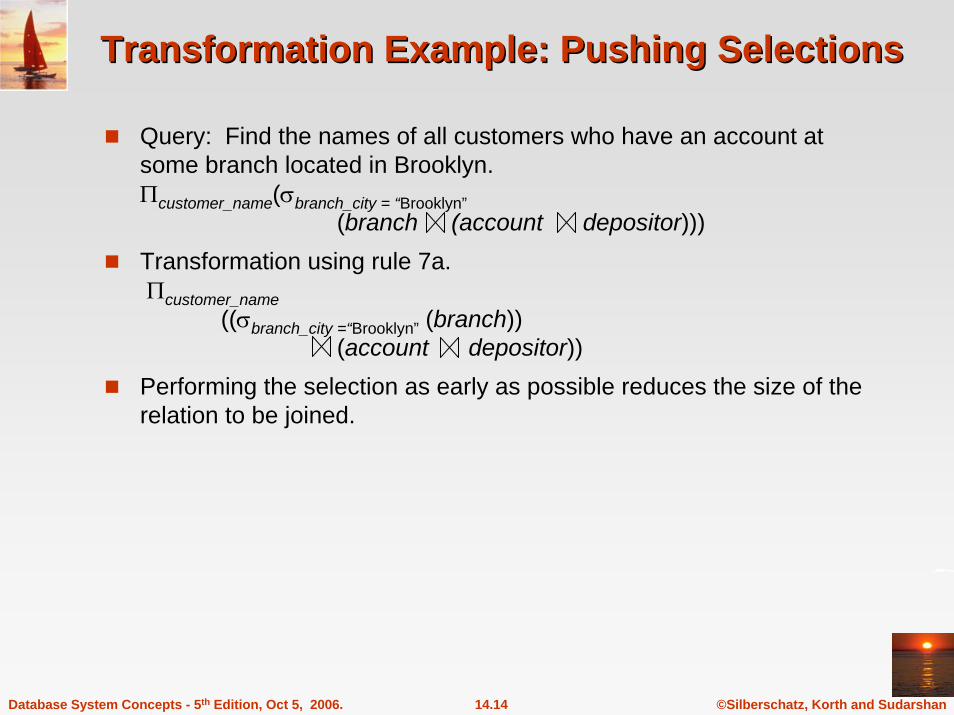
Query: Find the names of all customers who have an account at some branch located in Brooklyn.Πcustomer_name(σbranch_city = “Brooklyn”

(branch (account depositor)))Transformation using rule 7a.Πcustomer_name

((σbranch_city =“Brooklyn” (branch)) (account depositor))

Performing the selection as early as possible reduces the size of the relation to be joined.


Example with Multiple TransformationsExample with Multiple Transformations

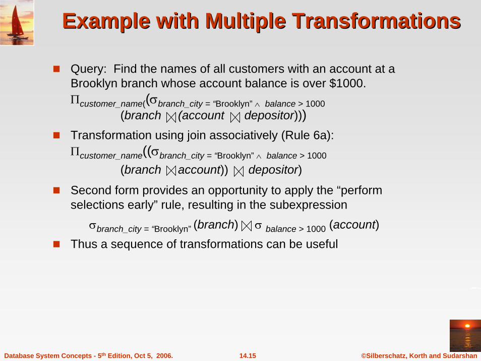
Query: Find the names of all customers with an account at a Brooklyn branch whose account balance is over $1000.Πcustomer_name((σbranch_city = “Brooklyn” ∧ balance > 1000

(branch (account depositor)))Transformation using join associatively (Rule 6a):Πcustomer_name((σbranch_city = “Brooklyn” ∧ balance > 1000

(branch account)) depositor)

Second form provides an opportunity to apply the “perform selections early” rule, resulting in the subexpression

σbranch_city = “Brooklyn” (branch) σ balance > 1000 (account)Thus a sequence of transformations can be useful


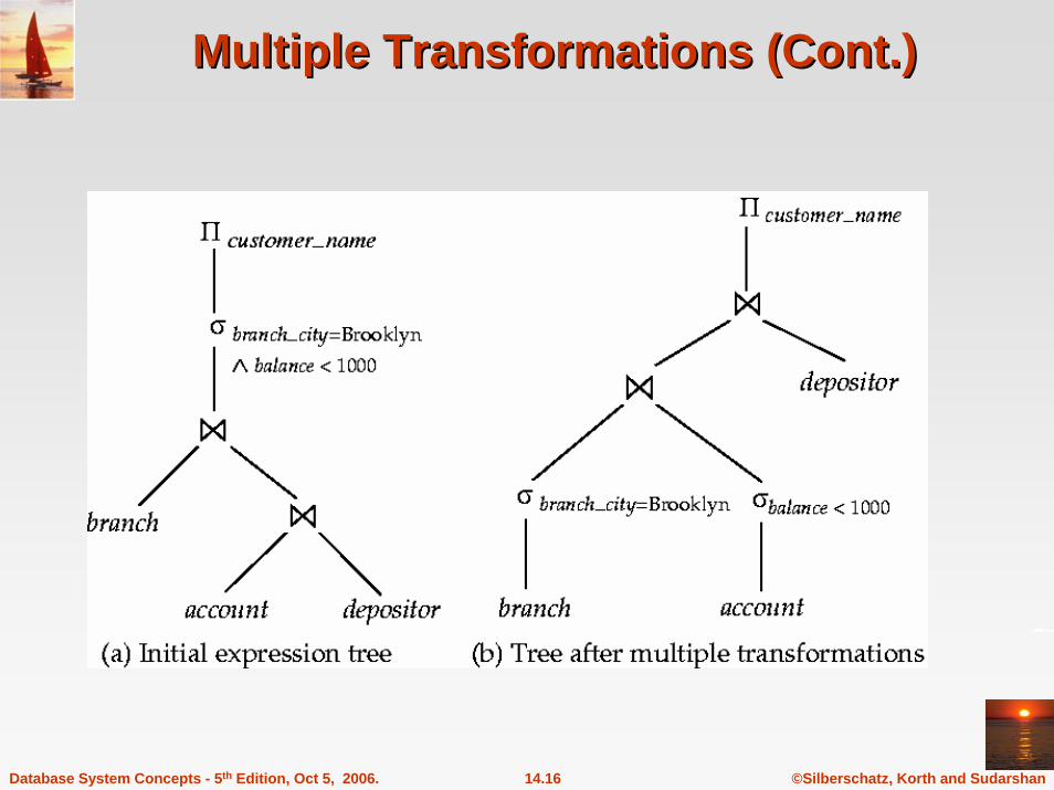
Multiple Transformations (Cont.)Multiple Transformations (Cont.)


Transformation Example: Pushing ProjectionsTransformation Example: Pushing Projections

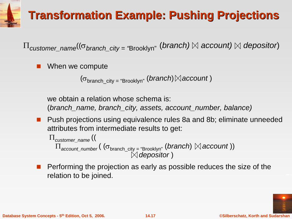
When we compute(σbranch_city = “Brooklyn” (branch) account )

we obtain a relation whose schema is:(branch_name, branch_city, assets, account_number, balance)Push projections using equivalence rules 8a and 8b; eliminate unneeded attributes from intermediate results to get:Πcustomer_name ((Πaccount_number ( (σbranch_city = “Brooklyn” (branch) account ))

depositor )Performing the projection as early as possible reduces the size of the relation to be joined.

Πcustomer_name((σbranch_city = “Brooklyn” (branch) account) depositor)


Join Ordering ExampleJoin Ordering Example

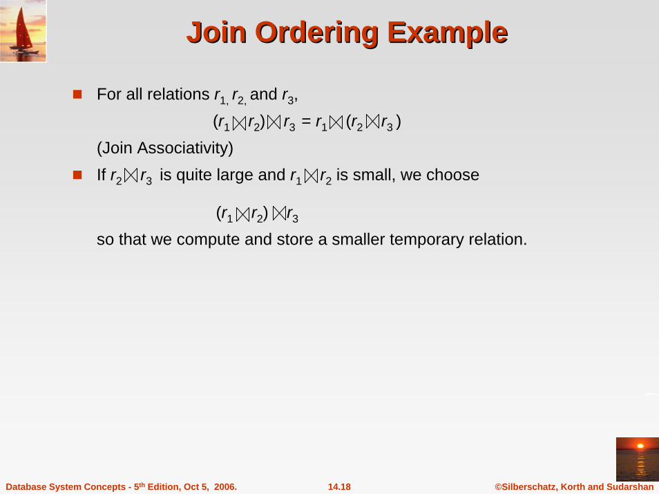
For all relations r1, r2, and r3,(r1 r2) r3 = r1 (r2 r3 )

(Join Associativity)If r2 r3 is quite large and r1 r2 is small, we choose

(r1 r2) r3

so that we compute and store a smaller temporary relation.


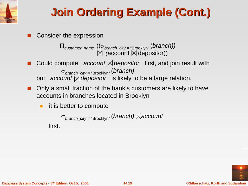
Join Ordering Example (Cont.)Join Ordering Example (Cont.)

Consider the expressionΠcustomer_name ((σbranch_city = “Brooklyn” (branch))

(account depositor))Could compute account depositor first, and join result with

σbranch_city = “Brooklyn” (branch)but account depositor is likely to be a large relation.Only a small fraction of the bank’s customers are likely to have accounts in branches located in Brooklyn

it is better to computeσbranch_city = “Brooklyn” (branch) account

first.


Enumeration of Equivalent ExpressionsEnumeration of Equivalent Expressions

Query optimizers use equivalence rules to systematically generate expressions equivalent to the given expressionCan generate all equivalent expressions as follows:

Repeatapply all applicable equivalence rules on every equivalent expression found so faradd newly generated expressions to the set of equivalent expressions

Until no new equivalent expressions are generated aboveThe above approach is very expensive in space and time

Two approachesOptimized plan generation based on transformation rulesSpecial case approach for queries with only selections, projections and joins


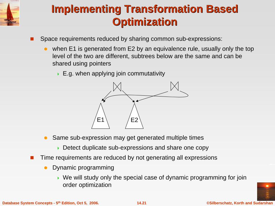
Implementing Transformation Based Implementing Transformation Based OptimizationOptimization

Space requirements reduced by sharing common sub-expressions:when E1 is generated from E2 by an equivalence rule, usually only the top level of the two are different, subtrees below are the same and can be shared using pointers

E.g. when applying join commutativity

Same sub-expression may get generated multiple timesDetect duplicate sub-expressions and share one copy

Time requirements are reduced by not generating all expressionsDynamic programming

We will study only the special case of dynamic programming for join order optimization

E1 E2


Cost EstimationCost Estimation

Cost of each operator computer as described in Chapter 13Need statistics of input relations

E.g. number of tuples, sizes of tuplesInputs can be results of sub-expressions

Need to estimate statistics of expression resultsTo do so, we require additional statistics

E.g. number of distinct values for an attributeMore on cost estimation later


Choice of Evaluation PlansChoice of Evaluation Plans

Must consider the interaction of evaluation techniques when choosing evaluation plans

choosing the cheapest algorithm for each operation independentlymay not yield best overall algorithm. E.g.

merge-join may be costlier than hash-join, but may provide a sorted output which reduces the cost for an outer level aggregation.nested-loop join may provide opportunity for pipelining

Practical query optimizers incorporate elements of the following two broad approaches:1. Search all the plans and choose the best plan in a

cost-based fashion.2. Uses heuristics to choose a plan.


CostCost--Based OptimizationBased Optimization

Consider finding the best join-order for r1 r2 . . . rn.There are (2(n – 1))!/(n – 1)! different join orders for above expression. With n = 7, the number is 665280, with n = 10, the number is greater than 176 billion!No need to generate all the join orders. Using dynamic programming, the least-cost join order for any subset of {r1, r2, . . . rn} is computed only once and stored for future use.


Dynamic Programming in OptimizationDynamic Programming in Optimization

To find best join tree for a set of n relations:To find best plan for a set S of n relations, consider all possible plans of the form: S1 (S – S1) where S1 is any non-empty subset of S.Recursively compute costs for joining subsets of S to find the cost of each plan. Choose the cheapest of the 2n – 1 alternatives.Base case for recursion: single relation access plan

Apply all selections on Ri using best choice of indices on Ri

When plan for any subset is computed, store it and reuse it when it is required again, instead of recomputing it

Dynamic programming


Join Order Optimization AlgorithmJoin Order Optimization Algorithm

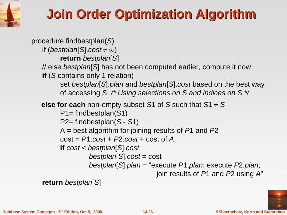
procedure findbestplan(S)if (bestplan[S].cost ≠ ∞)

return bestplan[S]// else bestplan[S] has not been computed earlier, compute it nowif (S contains only 1 relation)

set bestplan[S].plan and bestplan[S].cost based on the best way of accessing S /* Using selections on S and indices on S */

else for each non-empty subset S1 of S such that S1 ≠ SP1= findbestplan(S1)P2= findbestplan(S - S1)A = best algorithm for joining results of P1 and P2cost = P1.cost + P2.cost + cost of Aif cost < bestplan[S].cost

bestplan[S].cost = costbestplan[S].plan = “execute P1.plan; execute P2.plan;

join results of P1 and P2 using A”return bestplan[S]


Left Deep Join TreesLeft Deep Join Trees

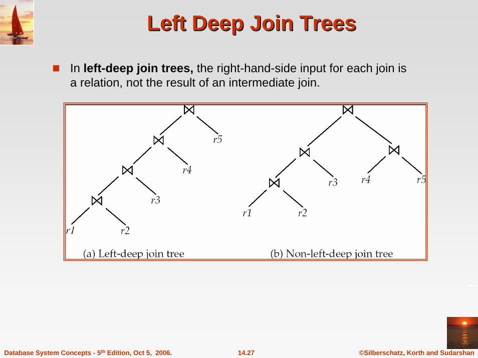
In left-deep join trees, the right-hand-side input for each join is a relation, not the result of an intermediate join.


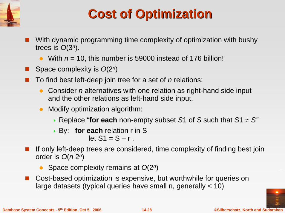
Cost of OptimizationCost of Optimization

With dynamic programming time complexity of optimization with bushy trees is O(3n).

With n = 10, this number is 59000 instead of 176 billion!Space complexity is O(2n) To find best left-deep join tree for a set of n relations:

Consider n alternatives with one relation as right-hand side input and the other relations as left-hand side input.Modify optimization algorithm:

Replace “for each non-empty subset S1 of S such that S1 ≠ S”By: for each relation r in S

let S1 = S – r .If only left-deep trees are considered, time complexity of finding best join order is O(n 2n)

Space complexity remains at O(2n) Cost-based optimization is expensive, but worthwhile for queries on large datasets (typical queries have small n, generally < 10)


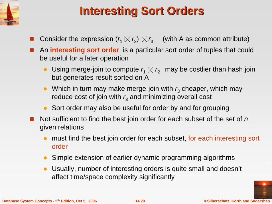
Interesting Sort OrdersInteresting Sort Orders

Consider the expression (r1 r2) r3 (with A as common attribute)An interesting sort order is a particular sort order of tuples that could be useful for a later operation

Using merge-join to compute r1 r2 may be costlier than hash join but generates result sorted on AWhich in turn may make merge-join with r3 cheaper, which may reduce cost of join with r3 and minimizing overall cost Sort order may also be useful for order by and for grouping

Not sufficient to find the best join order for each subset of the set of ngiven relations

must find the best join order for each subset, for each interesting sort orderSimple extension of earlier dynamic programming algorithmsUsually, number of interesting orders is quite small and doesn’t affect time/space complexity significantly


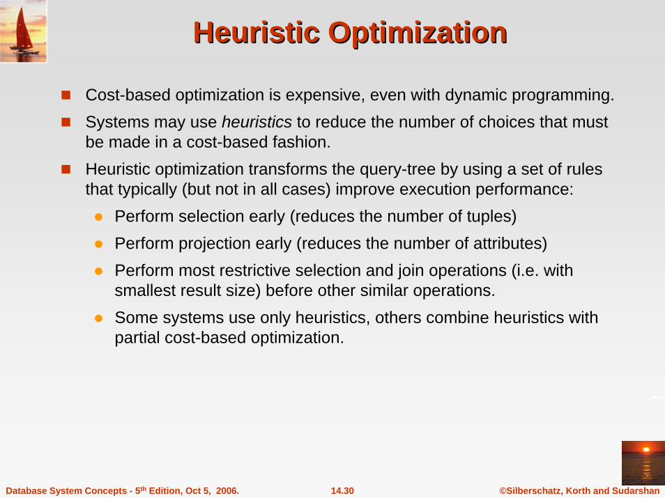
Heuristic OptimizationHeuristic Optimization

Cost-based optimization is expensive, even with dynamic programming.Systems may use heuristics to reduce the number of choices that must be made in a cost-based fashion.Heuristic optimization transforms the query-tree by using a set of rules that typically (but not in all cases) improve execution performance:

Perform selection early (reduces the number of tuples)Perform projection early (reduces the number of attributes)Perform most restrictive selection and join operations (i.e. with smallest result size) before other similar operations.Some systems use only heuristics, others combine heuristics withpartial cost-based optimization.


Structure of Query OptimizersStructure of Query Optimizers

Many optimizers considers only left-deep join orders.Plus heuristics to push selections and projections down the query treeReduces optimization complexity and generates plans amenable to pipelined evaluation.

Heuristic optimization used in some versions of Oracle:Repeatedly pick “best” relation to join next

Starting from each of n starting points. Pick best among theseIntricacies of SQL complicate query optimization

E.g. nested subqueries


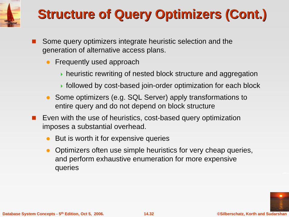
Structure of Query Optimizers (Cont.)Structure of Query Optimizers (Cont.)

Some query optimizers integrate heuristic selection and the generation of alternative access plans.

Frequently used approachheuristic rewriting of nested block structure and aggregationfollowed by cost-based join-order optimization for each block

Some optimizers (e.g. SQL Server) apply transformations to entire query and do not depend on block structure

Even with the use of heuristics, cost-based query optimization imposes a substantial overhead.

But is worth it for expensive queriesOptimizers often use simple heuristics for very cheap queries, and perform exhaustive enumeration for more expensive queries



Statistics for Cost EstimationStatistics for Cost Estimation


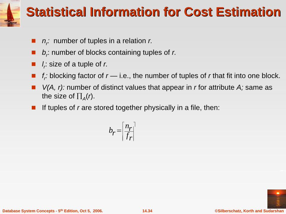
Statistical Information for Cost EstimationStatistical Information for Cost Estimation

nr: number of tuples in a relation r.br: number of blocks containing tuples of r.lr: size of a tuple of r.fr: blocking factor of r — i.e., the number of tuples of r that fit into one block.V(A, r): number of distinct values that appear in r for attribute A; same as the size of ∏A(r).If tuples of r are stored together physically in a file, then:

⎥⎥⎥

⎥

⎤

⎢⎢⎢

⎢

⎡=

rfrn

rb


HistogramsHistograms

Histogram on attribute age of relation person

Equi-width histogramsEqui-depth histograms


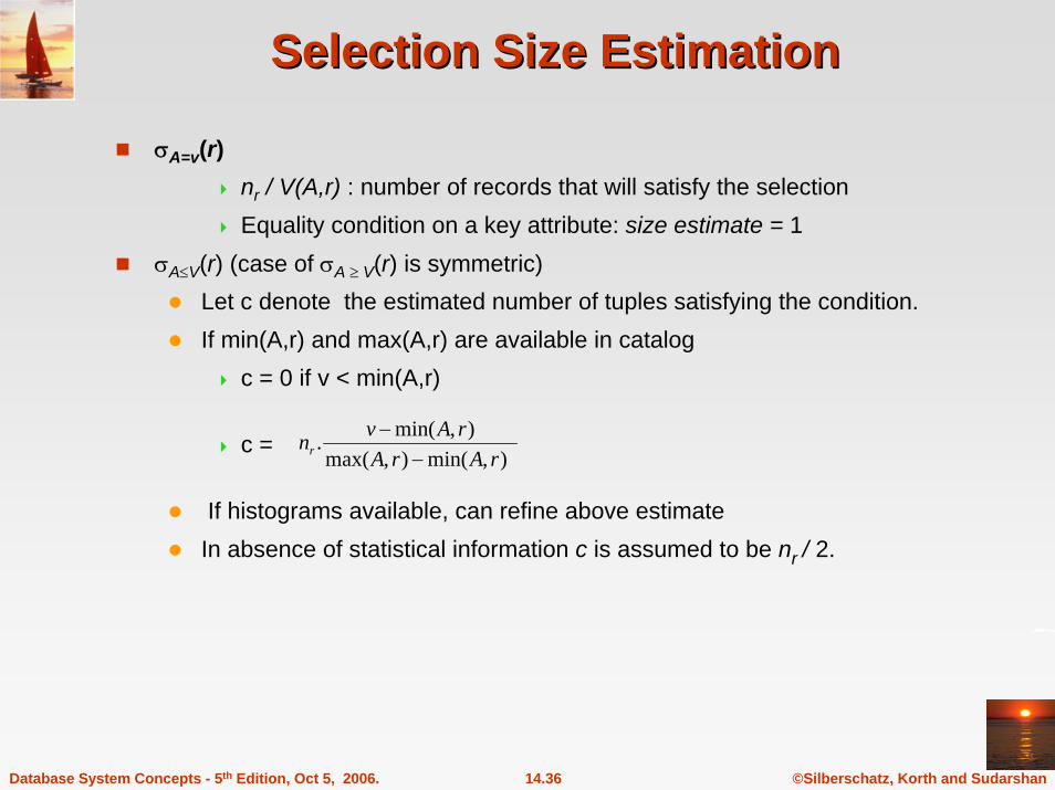
Selection Size EstimationSelection Size Estimation

σA=v(r)nr / V(A,r) : number of records that will satisfy the selectionEquality condition on a key attribute: size estimate = 1

σA≤V(r) (case of σA ≥ V(r) is symmetric)Let c denote the estimated number of tuples satisfying the condition. If min(A,r) and max(A,r) are available in catalog

c = 0 if v < min(A,r)

c =

If histograms available, can refine above estimateIn absence of statistical information c is assumed to be nr / 2.

),min(),max(),min(.

rArArAvnr −

−


Size Estimation of Complex SelectionsSize Estimation of Complex Selections

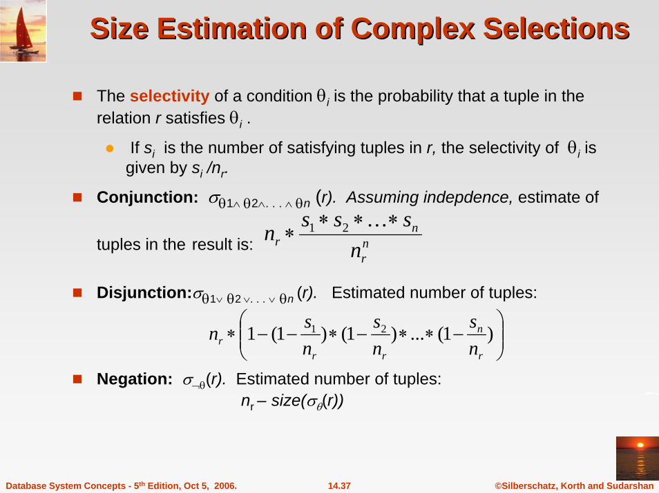
The selectivity of a condition θi is the probability that a tuple in the relation r satisfies θi .

If si is the number of satisfying tuples in r, the selectivity of θi is given by si /nr.

Conjunction: σθ1∧ θ2∧. . . ∧ θn (r). Assuming indepdence, estimate of

tuples in the result is:

Disjunction:σθ1∨ θ2 ∨. . . ∨ θn (r). Estimated number of tuples:

Negation: σ¬θ(r). Estimated number of tuples:nr – size(σθ(r))

nr

nr n

sssn ∗∗∗∗

. . . 21

⎟⎟⎠

⎞⎜⎜⎝

⎛−∗∗−∗−−∗ )1(...)1()1(1 21

r

n

rrr n

sns

nsn


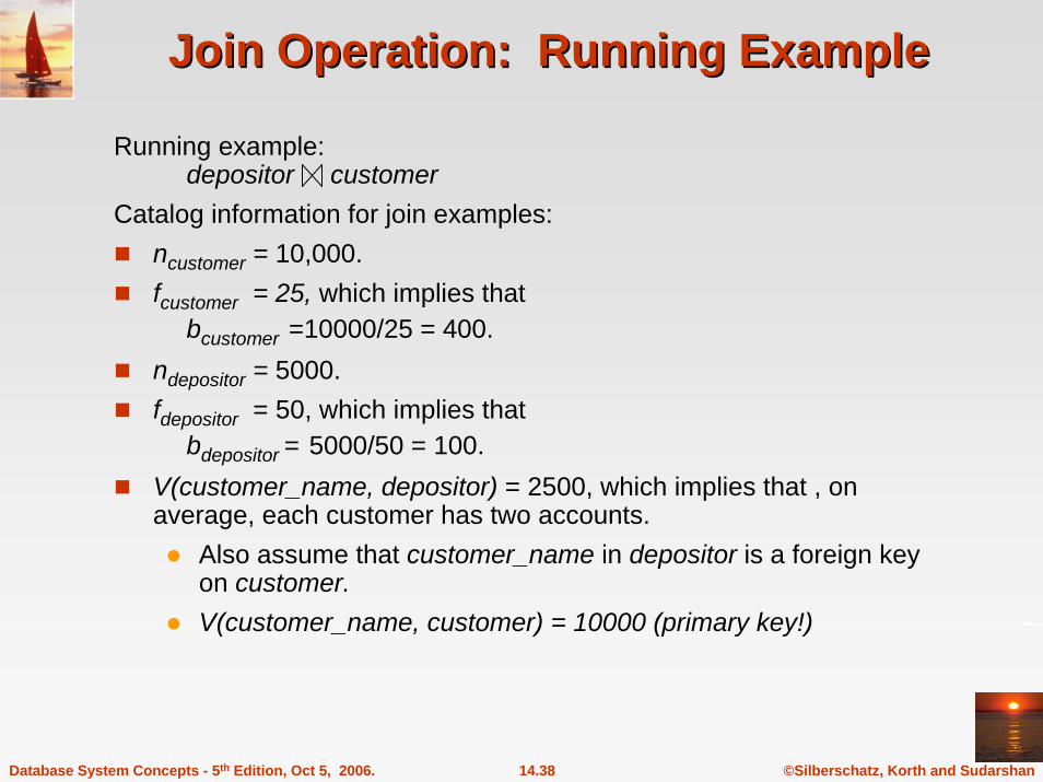
Join Operation: Running ExampleJoin Operation: Running Example

Running example: depositor customer

Catalog information for join examples:ncustomer = 10,000.fcustomer = 25, which implies that

bcustomer =10000/25 = 400.ndepositor = 5000.fdepositor = 50, which implies that

bdepositor = 5000/50 = 100.V(customer_name, depositor) = 2500, which implies that , on average, each customer has two accounts.

Also assume that customer_name in depositor is a foreign key on customer.V(customer_name, customer) = 10000 (primary key!)


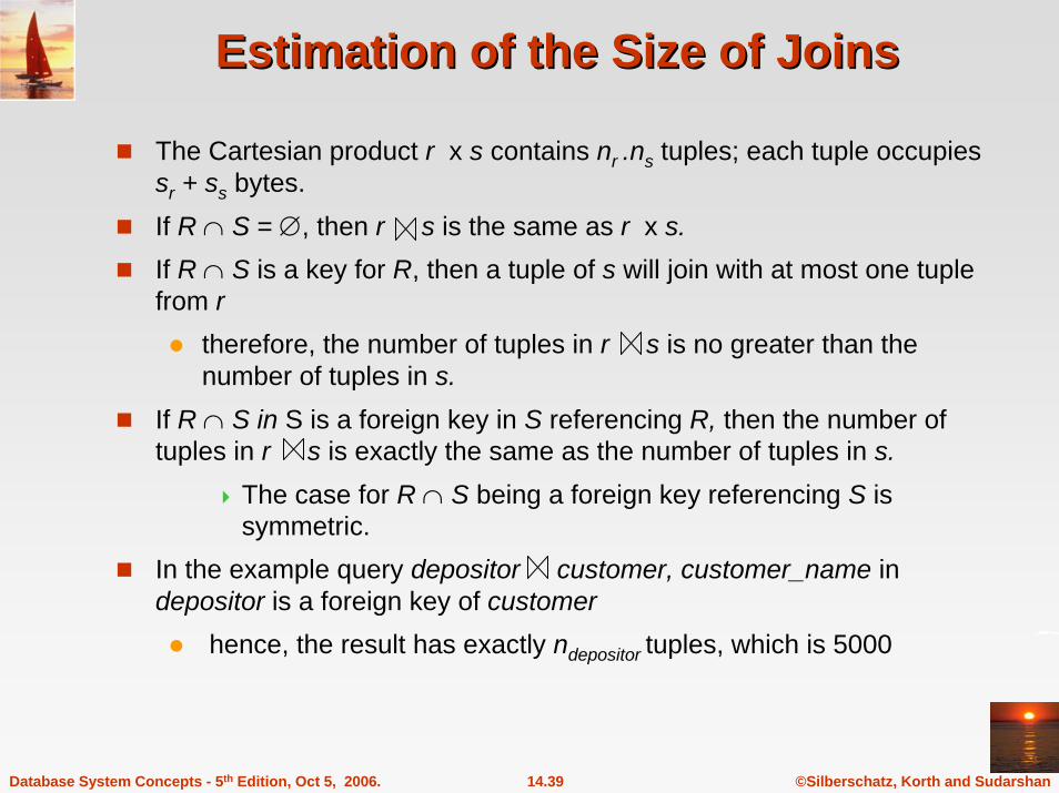
Estimation of the Size of JoinsEstimation of the Size of Joins

The Cartesian product r x s contains nr .ns tuples; each tuple occupies sr + ss bytes.If R ∩ S = ∅, then r s is the same as r x s. If R ∩ S is a key for R, then a tuple of s will join with at most one tuple from r

therefore, the number of tuples in r s is no greater than the number of tuples in s.

If R ∩ S in S is a foreign key in S referencing R, then the number of tuples in r s is exactly the same as the number of tuples in s.

The case for R ∩ S being a foreign key referencing S is symmetric.

In the example query depositor customer, customer_name in depositor is a foreign key of customer

hence, the result has exactly ndepositor tuples, which is 5000


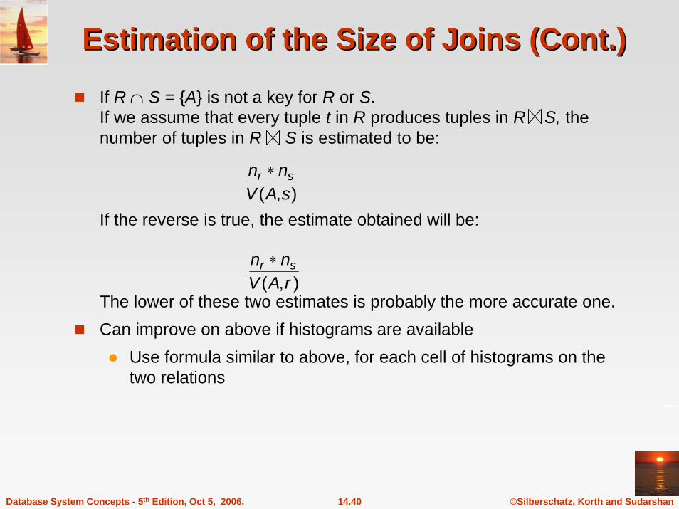
Estimation of the Size of Joins (Cont.)Estimation of the Size of Joins (Cont.)

If R ∩ S = {A} is not a key for R or S.If we assume that every tuple t in R produces tuples in R S, the number of tuples in R S is estimated to be:

If the reverse is true, the estimate obtained will be:

The lower of these two estimates is probably the more accurate one.Can improve on above if histograms are available

Use formula similar to above, for each cell of histograms on thetwo relations

),( sAVnn sr ∗

),( rAVnn sr ∗


Estimation of the Size of Joins (Cont.)Estimation of the Size of Joins (Cont.)

Compute the size estimates for depositor customer without using information about foreign keys:

V(customer_name, depositor) = 2500, andV(customer_name, customer) = 10000The two estimates are 5000 * 10000/2500 - 20,000 and 5000 * 10000/10000 = 5000We choose the lower estimate, which in this case, is the same asour earlier computation using foreign keys.


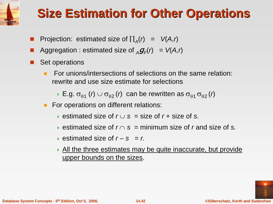
Size Estimation for Other OperationsSize Estimation for Other Operations

Projection: estimated size of ∏A(r) = V(A,r)Aggregation : estimated size of AgF(r) = V(A,r)

Set operationsFor unions/intersections of selections on the same relation: rewrite and use size estimate for selections

E.g. σθ1 (r) ∪ σθ2 (r) can be rewritten as σθ1 σθ2 (r)For operations on different relations:

estimated size of r ∪ s = size of r + size of s. estimated size of r ∩ s = minimum size of r and size of s.estimated size of r – s = r.All the three estimates may be quite inaccurate, but provide upper bounds on the sizes.


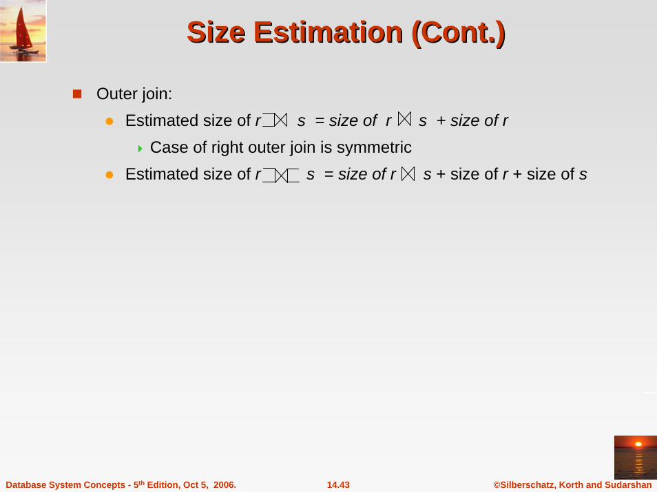
Size Estimation (Cont.)Size Estimation (Cont.)

Outer join: Estimated size of r s = size of r s + size of r

Case of right outer join is symmetricEstimated size of r s = size of r s + size of r + size of s


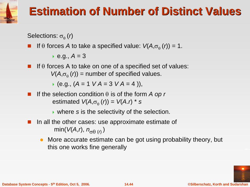
Estimation of Number of Distinct ValuesEstimation of Number of Distinct Values

Selections: σθ (r) If θ forces A to take a specified value: V(A,σθ (r)) = 1.

e.g., A = 3If θ forces A to take on one of a specified set of values:

V(A,σθ (r)) = number of specified values.(e.g., (A = 1 V A = 3 V A = 4 )),

If the selection condition θ is of the form A op restimated V(A,σθ (r)) = V(A.r) * s

where s is the selectivity of the selection.In all the other cases: use approximate estimate of

min(V(A,r), nσθ (r) )More accurate estimate can be got using probability theory, but this one works fine generally


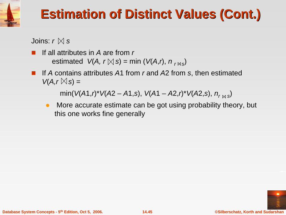
Estimation of Distinct Values (Cont.)Estimation of Distinct Values (Cont.)

Joins: r sIf all attributes in A are from r

estimated V(A, r s) = min (V(A,r), n r s)If A contains attributes A1 from r and A2 from s, then estimated V(A,r s) =

min(V(A1,r)*V(A2 – A1,s), V(A1 – A2,r)*V(A2,s), nr s)More accurate estimate can be got using probability theory, butthis one works fine generally


Estimation of Distinct Values (Cont.)Estimation of Distinct Values (Cont.)

Estimation of distinct values are straightforward for projections.They are the same in ∏A (r) as in r.

The same holds for grouping attributes of aggregation.For aggregated values

For min(A) and max(A), the number of distinct values can be estimated as min(V(A,r), V(G,r)) where G denotes grouping attributesFor other aggregates, assume all values are distinct, and use V(G,r)



Additional Optimization TechniquesAdditional Optimization Techniques

Nested SubqueriesMaterialized Views


Optimizing Nested Subqueries**Optimizing Nested Subqueries**

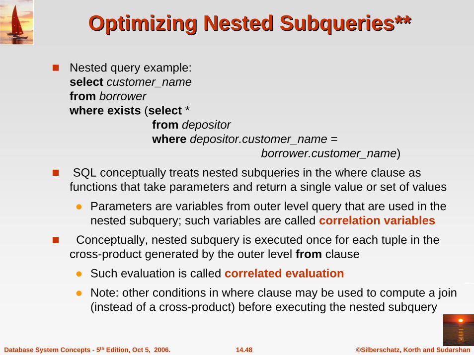
Nested query example:select customer_namefrom borrowerwhere exists (select *

from depositorwhere depositor.customer_name =

borrower.customer_name)SQL conceptually treats nested subqueries in the where clause as functions that take parameters and return a single value or set of values

Parameters are variables from outer level query that are used in the nested subquery; such variables are called correlation variables

Conceptually, nested subquery is executed once for each tuple in the cross-product generated by the outer level from clause

Such evaluation is called correlated evaluation Note: other conditions in where clause may be used to compute a join (instead of a cross-product) before executing the nested subquery


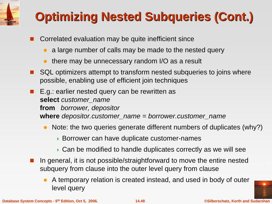
Optimizing Nested Subqueries (Cont.)Optimizing Nested Subqueries (Cont.)Correlated evaluation may be quite inefficient since

a large number of calls may be made to the nested query there may be unnecessary random I/O as a result

SQL optimizers attempt to transform nested subqueries to joins where possible, enabling use of efficient join techniquesE.g.: earlier nested query can be rewritten as select customer_namefrom borrower, depositorwhere depositor.customer_name = borrower.customer_name

Note: the two queries generate different numbers of duplicates (why?)Borrower can have duplicate customer-namesCan be modified to handle duplicates correctly as we will see

In general, it is not possible/straightforward to move the entire nested subquery from clause into the outer level query from clause

A temporary relation is created instead, and used in body of outer level query


Optimizing Nested Subqueries (Cont.)Optimizing Nested Subqueries (Cont.)

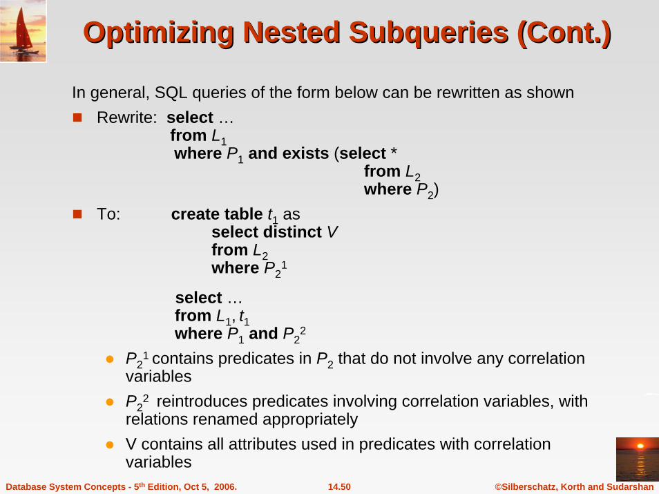
In general, SQL queries of the form below can be rewritten as shownRewrite: select …

from L1where P1 and exists (select *

from L2where P2)

To: create table t1 asselect distinct Vfrom L2where P2

1

select …from L1, t1where P1 and P2

2

P21 contains predicates in P2 that do not involve any correlation

variablesP2

2 reintroduces predicates involving correlation variables, with relations renamed appropriatelyV contains all attributes used in predicates with correlation variables


Optimizing Nested Subqueries (Cont.)Optimizing Nested Subqueries (Cont.)

In our example, the original nested query would be transformed tocreate table t1 as

select distinct customer_namefrom depositor

select customer_namefrom borrower, t1where t1.customer_name = borrower.customer_name

The process of replacing a nested query by a query with a join (possibly with a temporary relation) is called decorrelation.Decorrelation is more complicated when

the nested subquery uses aggregation, orwhen the result of the nested subquery is used to test for equality, or when the condition linking the nested subquery to the other query is not exists, and so on.


Materialized Views**Materialized Views**

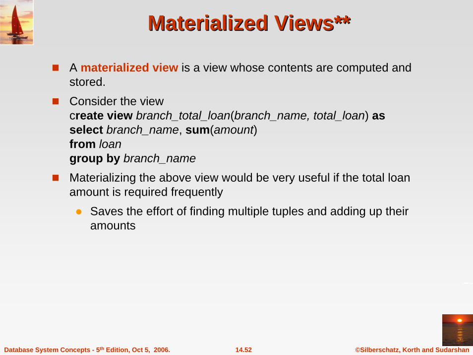
A materialized view is a view whose contents are computed and stored.Consider the viewcreate view branch_total_loan(branch_name, total_loan) asselect branch_name, sum(amount)from loangroup by branch_nameMaterializing the above view would be very useful if the total loan amount is required frequently

Saves the effort of finding multiple tuples and adding up their amounts


Materialized View MaintenanceMaterialized View Maintenance

The task of keeping a materialized view up-to-date with the underlying data is known as materialized view maintenanceMaterialized views can be maintained by recomputation on every updateA better option is to use incremental view maintenance

Changes to database relations are used to compute changes to the materialized view, which is then updated

View maintenance can be done byManually defining triggers on insert, delete, and update of eachrelation in the view definitionManually written code to update the view whenever database relations are updatedPeriodic recomputation (e.g. nightly)Above methods are directly supported by many database systems

Avoids manual effort/correctness issues


Incremental View MaintenanceIncremental View Maintenance

The changes (inserts and deletes) to a relation or expressions are referred to as its differential

Set of tuples inserted to and deleted from r are denoted ir and drTo simplify our description, we only consider inserts and deletes

We replace updates to a tuple by deletion of the tuple followed by insertion of the update tuple

We describe how to compute the change to the result of each relational operation, given changes to its inputsWe then outline how to handle relational algebra expressions


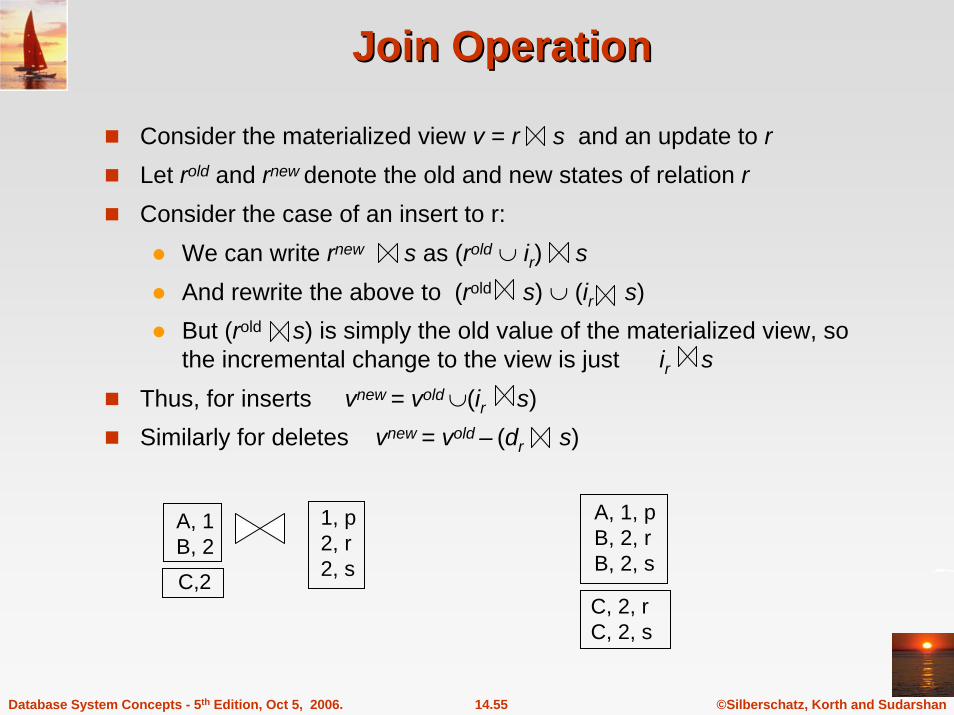
Join OperationJoin Operation

Consider the materialized view v = r s and an update to rLet rold and rnew denote the old and new states of relation rConsider the case of an insert to r:

We can write rnew s as (rold ∪ ir) sAnd rewrite the above to (rold s) ∪ (ir s)But (rold s) is simply the old value of the materialized view, so the incremental change to the view is just ir s

Thus, for inserts vnew = vold∪(ir s)Similarly for deletes vnew = vold – (dr s)

A, 1B, 2

1, p2, r2, s

A, 1, pB, 2, rB, 2, s

C,2C, 2, rC, 2, s


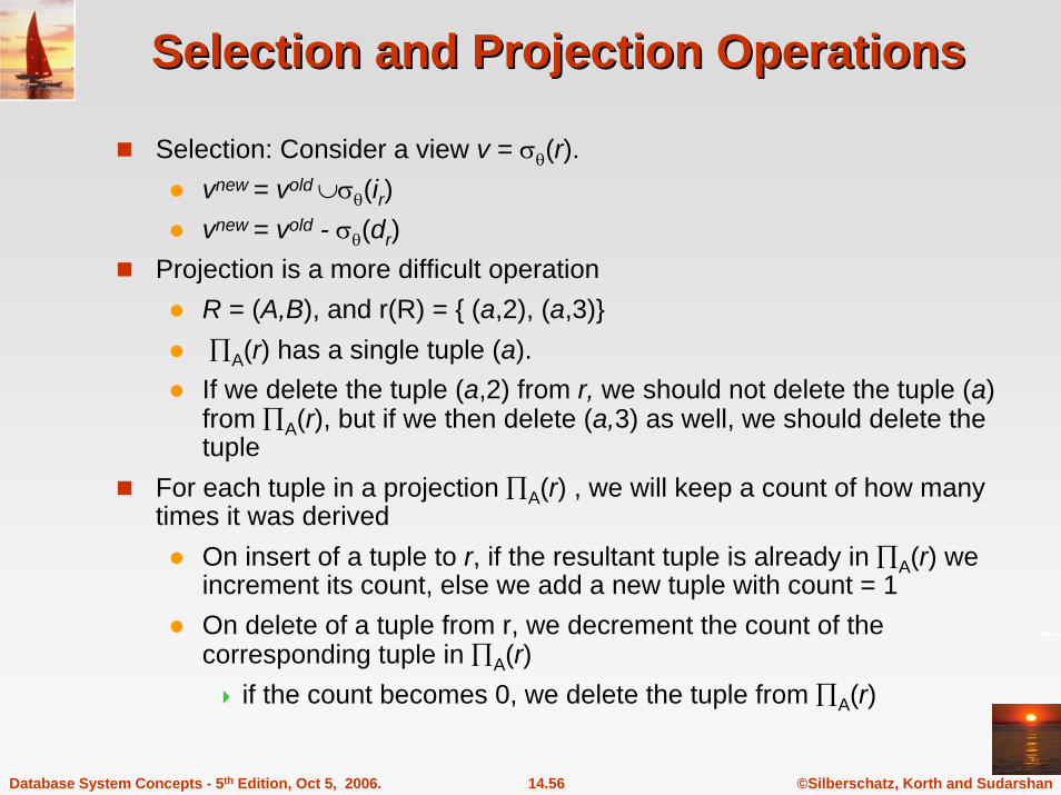
Selection and Projection OperationsSelection and Projection Operations

Selection: Consider a view v = σθ(r).vnew = vold ∪σθ(ir)vnew = vold - σθ(dr)

Projection is a more difficult operation R = (A,B), and r(R) = { (a,2), (a,3)}∏A(r) has a single tuple (a). If we delete the tuple (a,2) from r, we should not delete the tuple (a) from ∏A(r), but if we then delete (a,3) as well, we should delete the tuple

For each tuple in a projection ∏A(r) , we will keep a count of how many times it was derived

On insert of a tuple to r, if the resultant tuple is already in ∏A(r) we increment its count, else we add a new tuple with count = 1On delete of a tuple from r, we decrement the count of the corresponding tuple in ∏A(r)

if the count becomes 0, we delete the tuple from ∏A(r)


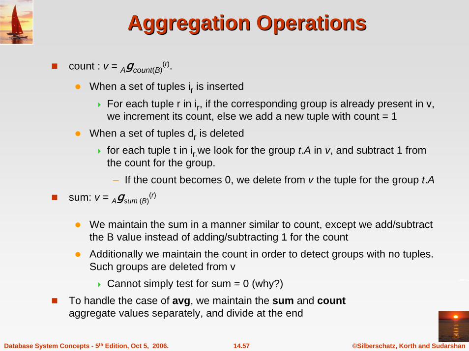
Aggregation OperationsAggregation Operations

count : v = Agcount(B)(r).

When a set of tuples ir is inserted For each tuple r in ir, if the corresponding group is already present in v, we increment its count, else we add a new tuple with count = 1

When a set of tuples dr is deletedfor each tuple t in ir.we look for the group t.A in v, and subtract 1 from the count for the group.

– If the count becomes 0, we delete from v the tuple for the group t.A

sum: v = Agsum (B)(r)

We maintain the sum in a manner similar to count, except we add/subtract the B value instead of adding/subtracting 1 for the countAdditionally we maintain the count in order to detect groups with no tuples. Such groups are deleted from v

Cannot simply test for sum = 0 (why?)To handle the case of avg, we maintain the sum and count aggregate values separately, and divide at the end


Aggregate Operations (Cont.)Aggregate Operations (Cont.)

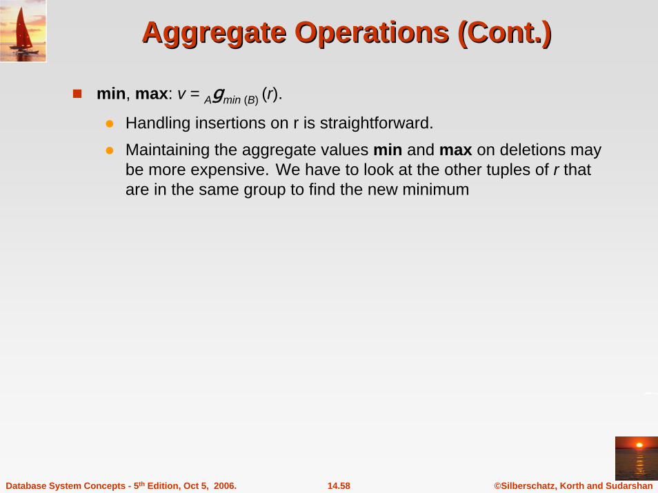
min, max: v = Agmin (B) (r).

Handling insertions on r is straightforward.Maintaining the aggregate values min and max on deletions may be more expensive. We have to look at the other tuples of r that are in the same group to find the new minimum


Other OperationsOther Operations

Set intersection: v = r ∩ swhen a tuple is inserted in r we check if it is present in s, and if so we add it to v. If the tuple is deleted from r, we delete it from the intersection if it is present. Updates to s are symmetricThe other set operations, union and set difference are handled in a similar fashion.

Outer joins are handled in much the same way as joins but with some extra work

we leave details to you.


Handling ExpressionsHandling Expressions

To handle an entire expression, we derive expressions for computing the incremental change to the result of each sub-expressions, starting from the smallest sub-expressions.E.g. consider E1 E2 where each of E1 and E2 may be a complex expression

Suppose the set of tuples to be inserted into E1 is given by D1

Computed earlier, since smaller sub-expressions are handled first

Then the set of tuples to be inserted into E1 E2 is given byD1 E2

This is just the usual way of maintaining joins


Query Optimization and Materialized ViewsQuery Optimization and Materialized Views

Rewriting queries to use materialized views:A materialized view v = r s is available A user submits a query r s tWe can rewrite the query as v t

Whether to do so depends on cost estimates for the two alternativeReplacing a use of a materialized view by the view definition:

A materialized view v = r s is available, but without any index on itUser submits a query σA=10(v). Suppose also that s has an index on the common attribute B, and r has an index on attribute A. The best plan for this query may be to replace v by r s, which can lead to the query plan σA=10(r) s

Query optimizer should be extended to consider all above alternatives and choose the best overall plan


Materialized View SelectionMaterialized View Selection

Materialized view selection: “What is the best set of views to materialize?”. Index selection: “what is the best set of indices to create”

closely related, to materialized view selectionbut simpler

Materialized view selection and index selection based on typicalsystem workload (queries and updates)

Typical goal: minimize time to execute workload , subject to constraints on space and time taken for some critical queries/updatesOne of the steps in database tuning

more on tuning in later chaptersCommercial database systems provide tools (called “tuning assistants” or “wizards”) to help the database administrator choose what indices and materialized views to create



Extra Slides:Extra Slides:Additional Optimization TechniquesAdditional Optimization Techniques

(see bibliographic notes)


TopTop--K QueriesK Queries

Top-K queriesselect * from r, swhere r.B = s.Border by r.A ascendinglimit 10Alternative 1: Indexed nested loops join with r as outerAlternative 2: estimate highest r.A value in result and add selection (and r.A <= H) to where clause

If < 10 results, retry with larger H


Optimization of UpdatesOptimization of Updates

Halloween problemupdate R set A = 5 * A where A > 10If index on A is used to find tuples satisfying A > 10, and tuples updated immediately, same tuple may be found (and updated) multiple timesSolution 1: Always defer updates

collect the updates (old and new values of tuples) and update relation and indices in second passDrawback: extra overhead even if e.g. update is only on R.B, not on attributes in selection condition

Solution 2: Defer only if requiredPerform immediate update if update does not affect attributes in where clause, and deferred updates otherwise.


Parametric Query OptimizationParametric Query Optimization

Example select * from r natural join swhere r.a < $1

value of parameter $1 not known at compile timeknown only at run time

different plans may be optimal for different values of $1Solution 1: optimize at run time, each time query is submitted

can be expensive Solution 2: Parametric Query Optimization:

optimizer generates a set of plans, optimal for different values of $1Set of optimal plans usually small for 1 to 3 parametersKey issue: how to do find set of optimal plans efficiently

best one from this set is chosen at run time when $1 is knownSolution 3: Query Plan Caching

If optimizer decides that same plan is likely to be optimal for all parameter values, it caches plan and reuses it, else reoptimize each timeImplemented in many database systems


Join MinimizationJoin Minimization

Join minimizationselect r.A, r.Bfrom r, swhere r.B = s.B

Check if join with s is redundant, drop it E.g. join condition is on foreign key from r to s, no selection on sOther sufficient conditions possible

select r.A, s1.B from r, s as s1, s as s2where r.B=s1.B and r.B = s2.B and s1.A < 20 and s2.A < 10

join with s2 is redundant and can be dropped (along with selection on s2)

Lots of research in this area since 70s/80s!


MultiqueryMultiquery OptimizationOptimizationExample

Q1: select * from (r natural join t) natural join sQ2: select * from (r natural join u) natural join s

Both queries share common subexpression (r natural join s)May be useful to compute (r natural join s) once and use it in both queries

But this may be more expensive in some situations– e.g. (r natural join s) may be expensive, plans as shown in queries

may be cheaperMultiquery optimization: find best overall plan for a set of queries, expoitingsharing of common subexpressions between queries where it is usefulSimple heuristic used in some database systems:

optimize each query separatelydetect and exploiting common subexpressions in the individual optimal query plans

May not always give best plan, but is cheap to implementSet of materialized views may share common subexpressions

As a result, view maintenance plans may share subexpressionsMultiquery optimization can be useful in such situations



End of ChapterEnd of Chapter

Documents

Chapter 14: Query Optimization - Yale Universitycodex.cs.yale.edu/avi/db-book/db5/slide-dir/ch14.pdf · Database System Concepts - 5th Edition, Oct 5, 2006. 14.2 ©Silberschatz, Korth