Chapter 2 - testbanklive.com · Microeconomics 8th Edition Pindyck Solutions Manual Full Download:

Copyright © 2013 Pearson Education. Inc. Publishing as Prentice Hall.

Chapter 2 The Basics of Supply and Demand

Teaching Notes

This chapter reviews the basics of supply and demand that students should be familiar with from their introductory economics courses. You may choose to spend more or less time on this chapter depending on how much review your students require. Chapter 2 departs from the standard treatment of supply and demand basics found in most other intermediate microeconomics textbooks by discussing many real-world markets (copper, office space in New York City, wheat, gasoline, natural gas, coffee, and others) and teaching students how to analyze these markets with the tools of supply and demand. The real-world applications are intended to show students the relevance of supply and demand analysis, and you may find it helpful to refer to these examples during class.

One of the most common problems students have in supply/demand analysis is confusion between a movement along a supply or demand curve and a shift in the curve. You should stress the ceteris paribus assumption, and explain that all variables except price are held constant along a supply or demand curve. So movements along the demand curve occur only with changes in price. When one of the omitted factors changes, the entire supply or demand curve shifts. You might find it useful to make up a simple linear demand function with quantity demanded on the left and the good’s price, a competing good’s price and income on the right. This gives you a chance to discuss substitutes and complements and also normal and inferior goods. Plug in values for the competing good’s price and income and plot the demand curve. Then change, say, the other good’s price and plot the demand curve again to show that it shifts. This demonstration helps students understand that the other variables are actually in the demand function and are merely lumped into the intercept term when we draw a demand curve. The same, of course, applies to supply curves as well.

It is important to make the distinction between quantity demanded as a function of price, QD = D(P), and the inverse demand function, P = D −1(QD), where price is a function of the quantity demanded. Since we plot price on the vertical axis, the inverse demand function is very useful. You can demonstrate this if you use an example as suggested above and plot the resulting demand curves. And, of course, there are “regular” and inverse supply curves as well.

Students also can have difficulties understanding how a market adjusts to a new equilibrium. They often think that the supply and/or demand curves shift as part of the equilibrium process. For example, suppose demand increases. Students typically recognize that price must increase, but some go on to say that supply will also have to increase to satisfy the increased level of demand. This may be a case of confusing an increase in quantity supplied with an increase in supply, but I have seen many students draw a shift in supply, so I try to get this cleared up as soon as possible.

The concept of elasticity, introduced in Section 2.4, is another source of problems. It is important to stress the fact that any elasticity is the ratio of two percentages. So, for example, if a firm’s product has a price elasticity of demand of −2, the firm can determine that a 5% increase in price will result in a 10% drop in sales. Use lots of concrete examples to convince students that firms and governments can make important

Microeconomics 8th Edition Pindyck Solutions ManualFull Download: http://testbanklive.com/download/microeconomics-8th-edition-pindyck-solutions-manual/

Full download all chapters instantly please go to Solutions Manual, Test Bank site: testbanklive.com

http://testbanklive.com/download/microeconomics-8th-edition-pindyck-solutions-manual/

Chapter 2 The Basics of Supply and Demand 9


use of elasticity information. A common source of confusion is the negative value for the price elasticity of demand. We often talk about it as if it were a positive number. The book is careful in referring to the “magnitude” of the price elasticity, by which it means the absolute value of the price elasticity, but students may not pick this up on their own. I warn students that I will speak of price elasticities as if they were positive numbers and will say that a good whose elasticity is −2 is more elastic (or greater) than one whose elasticity is −1, even though the mathematically inclined may cringe.

Section 2.6 brings a lot of this material together because elasticities are used to derive demand and supply curves, market equilibria are computed, curves are shifted, and new equilibria are determined. This shows students how we can estimate the quantitative (not just the qualitative) effects of, say, a disruption in oil supply as in Example 2.9. Unfortunately, this section takes some time to cover, especially if your students’ algebra is rusty. You’ll have to decide whether the benefits outweigh the costs.

Price controls are introduced in Section 2.7. Students usually don’t realize the full effects of price controls. They think only of the initial effect on prices without realizing that shortages or surpluses are created, so this is an important topic. However, the coverage here is quite brief. Chapter 9 examines the effects of price controls and other forms of government intervention in much greater detail, so you may want to defer this topic until then.

Questions for Review

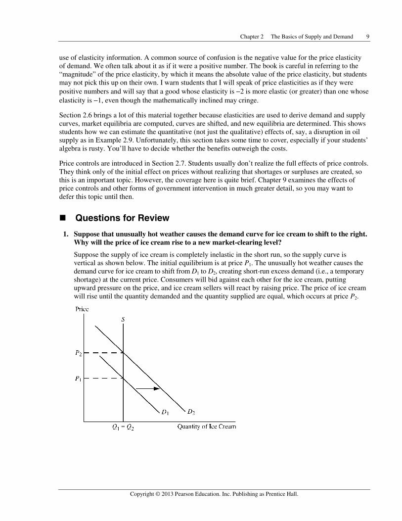
1. Suppose that unusually hot weather causes the demand curve for ice cream to shift to the right. Why will the price of ice cream rise to a new market-clearing level?

Suppose the supply of ice cream is completely inelastic in the short run, so the supply curve is vertical as shown below. The initial equilibrium is at price P1. The unusually hot weather causes the demand curve for ice cream to shift from D1 to D2, creating short-run excess demand (i.e., a temporary shortage) at the current price. Consumers will bid against each other for the ice cream, putting upward pressure on the price, and ice cream sellers will react by raising price. The price of ice cream will rise until the quantity demanded and the quantity supplied are equal, which occurs at price P2.

10 Pindyck/Rubinfeld, Microeconomics, Eighth Edition


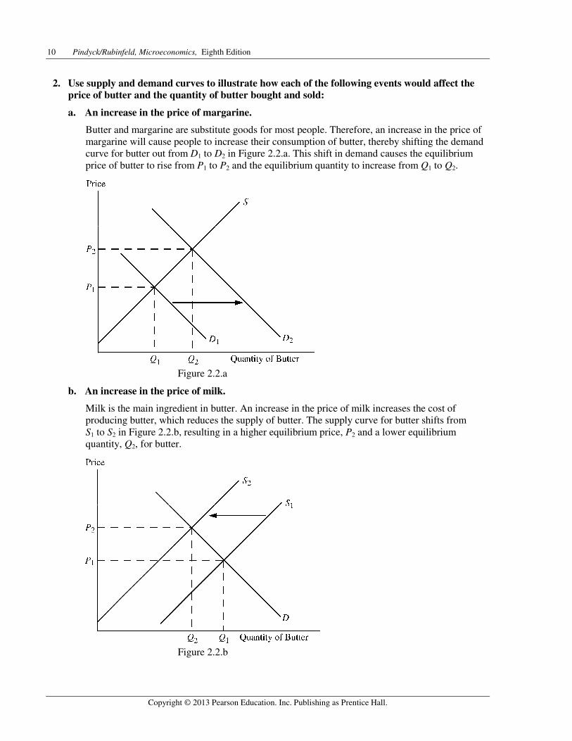
2. Use supply and demand curves to illustrate how each of the following events would affect the price of butter and the quantity of butter bought and sold:

a. An increase in the price of margarine.

Butter and margarine are substitute goods for most people. Therefore, an increase in the price of margarine will cause people to increase their consumption of butter, thereby shifting the demand curve for butter out from D1 to D2 in Figure 2.2.a. This shift in demand causes the equilibrium price of butter to rise from P1 to P2 and the equilibrium quantity to increase from Q1 to Q2.

Figure 2.2.a

b. An increase in the price of milk.

Milk is the main ingredient in butter. An increase in the price of milk increases the cost of producing butter, which reduces the supply of butter. The supply curve for butter shifts from S1 to S2 in Figure 2.2.b, resulting in a higher equilibrium price, P2 and a lower equilibrium quantity, Q2, for butter.

Figure 2.2.b



Note: Butter is in fact made from the fat that is skimmed from milk; thus butter and milk are joint products, and this complicates things. If you take account of this relationship, your answer might change, but it depends on why the price of milk increased. If the increase were caused by an increase in the demand for milk, the equilibrium quantity of milk supplied would increase. With more milk being produced, there would be more milk fat available to make butter, and the price of milk fat would fall. This would shift the supply curve for butter to the right, resulting in a drop in the price of butter and an increase in the quantity of butter supplied.

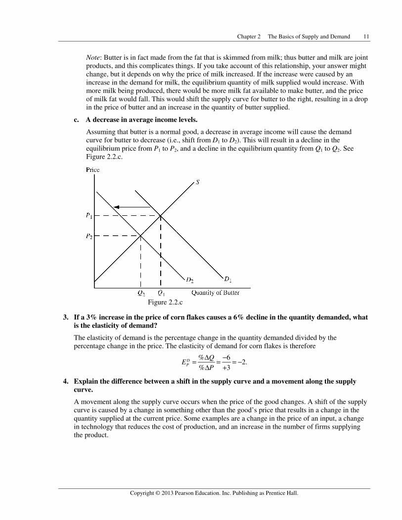
c. A decrease in average income levels.

Assuming that butter is a normal good, a decrease in average income will cause the demand curve for butter to decrease (i.e., shift from D1 to D2). This will result in a decline in the equilibrium price from P1 to P2, and a decline in the equilibrium quantity from Q1 to Q2. See Figure 2.2.c.

Figure 2.2.c

3. If a 3% increase in the price of corn flakes causes a 6% decline in the quantity demanded, what is the elasticity of demand?

The elasticity of demand is the percentage change in the quantity demanded divided by the percentage change in the price. The elasticity of demand for corn flakes is therefore

% 62.

% 3DP

QE

P

Δ −= = = −Δ +

4. Explain the difference between a shift in the supply curve and a movement along the supply curve.

A movement along the supply curve occurs when the price of the good changes. A shift of the supply curve is caused by a change in something other than the good’s price that results in a change in the quantity supplied at the current price. Some examples are a change in the price of an input, a change in technology that reduces the cost of production, and an increase in the number of firms supplying the product.



5. Explain why for many goods, the long-run price elasticity of supply is larger than the short-run elasticity.

The price elasticity of supply is the percentage change in the quantity supplied divided by the percentage change in price. In the short run, an increase in price induces firms to produce more by using their facilities more hours per week, paying workers to work overtime and hiring new workers. Nevertheless, there is a limit to how much firms can produce because they face capacity constraints in the short run. In the long run, however, firms can expand capacity by building new plants and hiring new permanent workers. Also, new firms can enter the market and add their output to total supply. Hence a greater change in quantity supplied is possible in the long run, and thus the price elasticity of supply is larger in the long run than in the short run.

6. Why do long-run elasticities of demand differ from short-run elasticities? Consider two goods: paper towels and televisions. Which is a durable good? Would you expect the price elasticity of demand for paper towels to be larger in the short run or in the long run? Why? What about the price elasticity of demand for televisions?

Long-run and short-run elasticities differ based on how rapidly consumers respond to price changes and how many substitutes are available. If the price of paper towels, a non-durable good, were to increase, consumers might react only minimally in the short run because it takes time for people to change their consumption habits. In the long run, however, consumers might learn to use other products such as sponges or kitchen towels instead of paper towels. Thus, the price elasticity would be larger in the long run than in the short run. In contrast, the quantity demanded of durable goods, such as televisions, might change dramatically in the short run. For example, the initial result of a price increase for televisions would cause consumers to delay purchases because they could keep on using their current TVs longer. Eventually consumers would replace their televisions as they wore out or became obsolete. Therefore, we expect the demand for durables to be more elastic in the short run than in the long run.

7. Are the following statements true or false? Explain your answers.

a. The elasticity of demand is the same as the slope of the demand curve.

False. Elasticity of demand is the percentage change in quantity demanded divided by the percentage change in the price of the product. In contrast, the slope of the demand curve is the change in quantity demanded (in units) divided by the change in price (typically in dollars). The difference is that elasticity uses percentage changes while the slope is based on changes in the number of units and number of dollars.

b. The cross-price elasticity will always be positive.

False. The cross-price elasticity measures the percentage change in the quantity demanded of one good due to a 1% change in the price of another good. This elasticity will be positive for substitutes (an increase in the price of hot dogs is likely to cause an increase in the quantity demanded of hamburgers) and negative for complements (an increase in the price of hot dogs is likely to cause a decrease in the quantity demanded of hot dog buns).

c. The supply of apartments is more inelastic in the short run than the long run.

True. In the short run it is difficult to change the supply of apartments in response to a change in price. Increasing the supply requires constructing new apartment buildings, which can take a year or more. Therefore, the elasticity of supply is more inelastic in the short run than in the long run.



8. Suppose the government regulates the prices of beef and chicken and sets them below their market-clearing levels. Explain why shortages of these goods will develop and what factors will determine the sizes of the shortages. What will happen to the price of pork? Explain briefly.

If the price of a commodity is set below its market-clearing level, the quantity that firms are willing to supply is less than the quantity that consumers wish to purchase. The extent of the resulting shortage depends on the elasticities of demand and supply as well as the amount by which the regulated price is set below the market-clearing price. For instance, if both supply and demand are elastic, the shortage is larger than if both are inelastic, and if the regulated price is substantially below the market-clearing price, the shortage is larger than if the regulated price is only slightly below the market-clearing price. Factors such as the willingness of consumers to eat less meat and the ability of farmers to reduce the size of their herds/flocks will determine the relevant elasticities. Customers whose demands for beef and chicken are not met because of the shortages will want to purchase substitutes like pork. This increases the demand for pork (i.e., shifts demand to the right), which results in a higher price for pork.

9. The city council of a small college town decides to regulate rents in order to reduce student living expenses. Suppose the average annual market-clearing rent for a two-bedroom apartment had been $700 per month and that rents were expected to increase to $900 within a year. The city council limits rents to their current $700-per-month level.

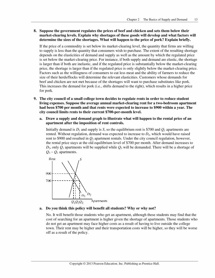
a. Draw a supply and demand graph to illustrate what will happen to the rental price of an apartment after the imposition of rent controls.

Initially demand is D1 and supply is S, so the equilibrium rent is $700 and Q1 apartments are rented. Without regulation, demand was expected to increase to D2, which would have raised rent to $900 and resulted in Q2 apartment rentals. Under the city council regulation, however, the rental price stays at the old equilibrium level of $700 per month. After demand increases to D2, only Q1 apartments will be supplied while Q3 will be demanded. There will be a shortage of Q3 − Q1 apartments.

a. Do you think this policy will benefit all students? Why or why not?

No. It will benefit those students who get an apartment, although these students may find that the cost of searching for an apartment is higher given the shortage of apartments. Those students who do not get an apartment may face higher costs as a result of having to live outside the college town. Their rent may be higher and their transportation costs will be higher, so they will be worse off as a result of the policy.



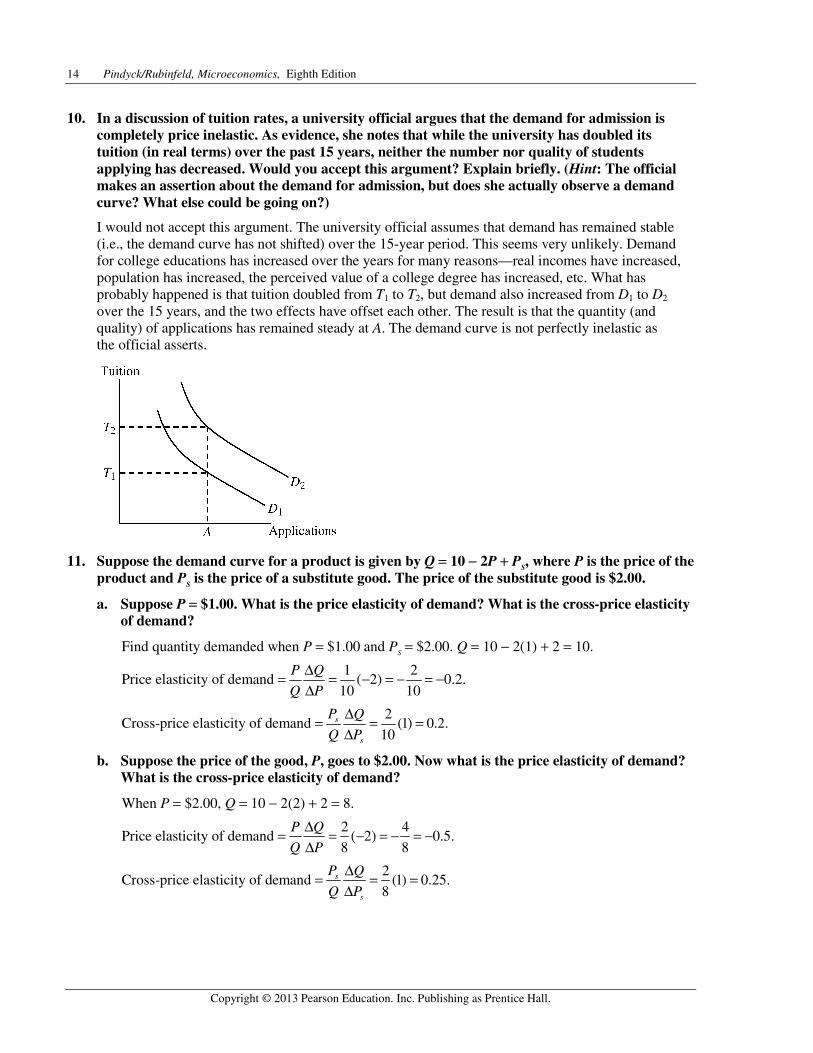
10. In a discussion of tuition rates, a university official argues that the demand for admission is completely price inelastic. As evidence, she notes that while the university has doubled its tuition (in real terms) over the past 15 years, neither the number nor quality of students applying has decreased. Would you accept this argument? Explain briefly. (Hint: The official makes an assertion about the demand for admission, but does she actually observe a demand curve? What else could be going on?)

I would not accept this argument. The university official assumes that demand has remained stable (i.e., the demand curve has not shifted) over the 15-year period. This seems very unlikely. Demand for college educations has increased over the years for many reasons—real incomes have increased, population has increased, the perceived value of a college degree has increased, etc. What has probably happened is that tuition doubled from T1 to T2, but demand also increased from D1 to D2 over the 15 years, and the two effects have offset each other. The result is that the quantity (and quality) of applications has remained steady at A. The demand curve is not perfectly inelastic as the official asserts.

11. Suppose the demand curve for a product is given by Q = 10 − 2P + PS, where P is the price of the product and PS is the price of a substitute good. The price of the substitute good is $2.00.

a. Suppose P = $1.00. What is the price elasticity of demand? What is the cross-price elasticity of demand?

Find quantity demanded when P = $1.00 and PS = $2.00. Q = 10 − 2(1) + 2 = 10.

Price elasticity of demand = 1 2

( 2) 0.2.10 10

P Q

Q P

Δ = − = − = −Δ

Cross-price elasticity of demand = 2

(1) 0.2.10

s

s

P Q

Q P

Δ = =Δ

b. Suppose the price of the good, P, goes to $2.00. Now what is the price elasticity of demand? What is the cross-price elasticity of demand?

When P = $2.00, Q = 10 − 2(2) + 2 = 8.

Price elasticity of demand = 2 4

( 2) 0.5.8 8

P Q

Q P

Δ = − = − = −Δ

Cross-price elasticity of demand = 2

(1) 0.25.8

s

s

P Q

Q P

Δ = =Δ



12. Suppose that rather than the declining demand assumed in Example 2.8, a decrease in the cost of copper production causes the supply curve to shift to the right by 40%. How will the price of copper change?

If the supply curve shifts to the right by 40% then the new quantity supplied will be 140% of the old quantity supplied at every price. The new supply curve is therefore the old supply curve multiplied by 1.4.

QS′ = 1.4 (−9 + 9P) = −12.6 + 12.6P. To find the new equilibrium price of copper, set the new supply equal to demand. Thus, –12.6 + 12.6P = 27 − 3P. Solving for price results in P = $2.54 per pound for the new equilibrium price. The price decreased by 46 cents per pound, from $3.00 to $2.54, a drop of about 15.3%.

13. Suppose the demand for natural gas is perfectly inelastic. What would be the effect, if any, of natural gas price controls?

If the demand for natural gas is perfectly inelastic, the demand curve is vertical. Consumers will demand the same quantity regardless of price. In this case, price controls will have no effect on the quantity demanded, but they will still cause a shortage if the supply curve is upward sloping and the regulated price is set below the market-clearing price, because suppliers will produce less natural gas than consumers wish to purchase.

Exercises

1. Suppose the demand curve for a product is given by Q = 300 − 2P + 4I, where I is average income measured in thousands of dollars. The supply curve is Q = 3P − 50.

a. If I = 25, find the market-clearing price and quantity for the product.

Given I = 25, the demand curve becomes Q = 300 − 2P + 4(25), or Q = 400 − 2P. Set demand equal to supply and solve for P and then Q:

400 − 2P = 3P − 50 P = 90 Q = 400 − 2(90) = 220.

b. If I = 50, find the market-clearing price and quantity for the product.

Given I = 50, the demand curve becomes Q = 300 − 2P + 4(50), or Q = 500 − 2P. Setting demand equal to supply, solve for P and then Q:

500 − 2P = 3P − 50 P = 110 Q = 500 − 2(110) = 280.

c. Draw a graph to illustrate your answers.

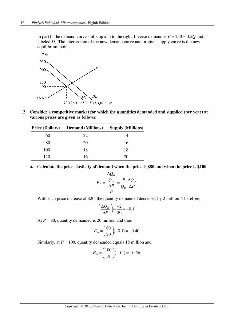
It is easier to draw the demand and supply curves if you first solve for the inverse demand and supply functions, i.e., solve the functions for P. Demand in part a is P = 200 − 0.5Q and supply is P = 16.67 + 0.333Q. These are shown on the graph as Da and S. Equilibrium price and quantity are found at the intersection of these demand and supply curves. When the income level increases



in part b, the demand curve shifts up and to the right. Inverse demand is P = 250 − 0.5Q and is labeled Db. The intersection of the new demand curve and original supply curve is the new equilibrium point.

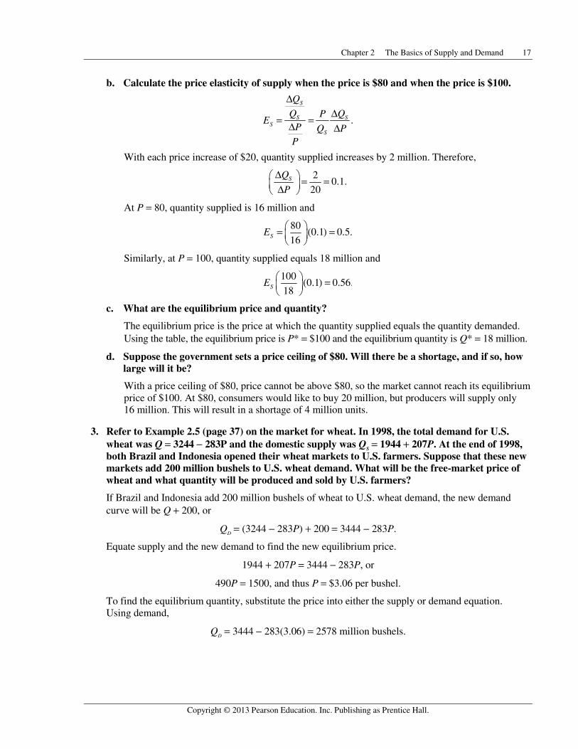
2. Consider a competitive market for which the quantities demanded and supplied (per year) at various prices are given as follows:

Price (Dollars) Demand (Millions) Supply (Millions)

60 22 14

80 20 16

100 18 18

120 16 20

a. Calculate the price elasticity of demand when the price is $80 and when the price is $100.

.

D

D DD

D

Q

Q QPE

P Q PP

ΔΔ= =

Δ Δ

With each price increase of $20, the quantity demanded decreases by 2 million. Therefore,

20.1.

20DQ

P

Δ − = = − Δ

At P = 80, quantity demanded is 20 million and thus

80( 0.1) 0.40.

20DE = − = −

Similarly, at P = 100, quantity demanded equals 18 million and

100( 0.1) 0.56.

18DE = − = −



b. Calculate the price elasticity of supply when the price is $80 and when the price is $100.

.

S

S SS

S

Q

Q QPE

P Q PP

ΔΔ= =

Δ Δ

With each price increase of $20, quantity supplied increases by 2 million. Therefore,

20.1.

20SQ

P

Δ = = Δ

At P = 80, quantity supplied is 16 million and

80(0.1) 0.5.

16SE = =

Similarly, at P = 100, quantity supplied equals 18 million and

100(0.1) 0.56.

18SE =

c. What are the equilibrium price and quantity?

The equilibrium price is the price at which the quantity supplied equals the quantity demanded. Using the table, the equilibrium price is P* = $100 and the equilibrium quantity is Q* = 18 million.

d. Suppose the government sets a price ceiling of $80. Will there be a shortage, and if so, how large will it be?

With a price ceiling of $80, price cannot be above $80, so the market cannot reach its equilibrium price of $100. At $80, consumers would like to buy 20 million, but producers will supply only 16 million. This will result in a shortage of 4 million units.

3. Refer to Example 2.5 (page 37) on the market for wheat. In 1998, the total demand for U.S. wheat was Q = 3244 − 283P and the domestic supply was QS = 1944 + 207P. At the end of 1998, both Brazil and Indonesia opened their wheat markets to U.S. farmers. Suppose that these new markets add 200 million bushels to U.S. wheat demand. What will be the free-market price of wheat and what quantity will be produced and sold by U.S. farmers?

If Brazil and Indonesia add 200 million bushels of wheat to U.S. wheat demand, the new demand curve will be Q + 200, or

QD = (3244 − 283P) + 200 = 3444 − 283P.

Equate supply and the new demand to find the new equilibrium price.

1944 + 207P = 3444 − 283P, or

490P = 1500, and thus P = $3.06 per bushel.

To find the equilibrium quantity, substitute the price into either the supply or demand equation. Using demand,

QD = 3444 − 283(3.06) = 2578 million bushels.



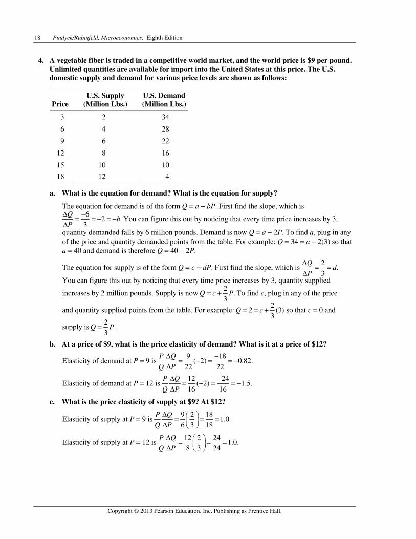
4. A vegetable fiber is traded in a competitive world market, and the world price is $9 per pound. Unlimited quantities are available for import into the United States at this price. The U.S. domestic supply and demand for various price levels are shown as follows:

Price U.S. Supply

(Million Lbs.) U.S. Demand (Million Lbs.)

3 2 34

6 4 28

9 6 22

12 8 16

15 10 10

18 12 4

a. What is the equation for demand? What is the equation for supply?

The equation for demand is of the form Q = a − bP. First find the slope, which is 6

2 .3

Qb

P

Δ −= = − = −Δ

You can figure this out by noticing that every time price increases by 3,

quantity demanded falls by 6 million pounds. Demand is now Q = a − 2P. To find a, plug in any of the price and quantity demanded points from the table. For example: Q = 34 = a − 2(3) so that a = 40 and demand is therefore Q = 40 − 2P.

The equation for supply is of the form Q = c + dP. First find the slope, which is 2

.3

Qd

P

Δ = =Δ

You can figure this out by noticing that every time price increases by 3, quantity supplied

increases by 2 million pounds. Supply is now 2

.3

Q c P= + To find c, plug in any of the price

and quantity supplied points from the table. For example: 2

2 (3)3

Q c= = + so that c = 0 and

supply is 2

.3

Q P=

b. At a price of $9, what is the price elasticity of demand? What is it at a price of $12?

Elasticity of demand at P = 9 is 9 18

( 2) 0.82.22 22

P Q

Q P

Δ −= − = = −Δ

Elasticity of demand at P = 12 is 12 24

( 2) 1.5.16 16

P Q

Q P

Δ −= − = = −Δ

c. What is the price elasticity of supply at $9? At $12?

Elasticity of supply at P = 9 is 9 2 18

1.0.6 3 18

P Q

Q P

Δ = = = Δ

Elasticity of supply at P = 12 is 12 2 24

1.0.8 3 24

P Q

Q P

Δ = = = Δ



d. In a free market, what will be the U.S. price and level of fiber imports?

With no restrictions on trade, the price in the United States will be the same as the world price, so P = $9. At this price, the domestic supply is 6 million lbs., while the domestic demand is 22 million lbs. Imports make up the difference and are 16 million lbs.

5. Much of the demand for U.S. agricultural output has come from other countries. In 1998, the total demand for wheat was Q = 3244 − 283P. Of this, total domestic demand was QD = 1700 − 107P, and domestic supply was QS = 1944 + 207P. Suppose the export demand for wheat falls by 40%.

a. U.S. farmers are concerned about this drop in export demand. What happens to the free-market price of wheat in the United States? Do farmers have much reason to worry?

Before the drop in export demand, the market equilibrium price is found by setting total demand equal to domestic supply:

3244 − 283P = 1944 + 207P, or

P = $2.65.

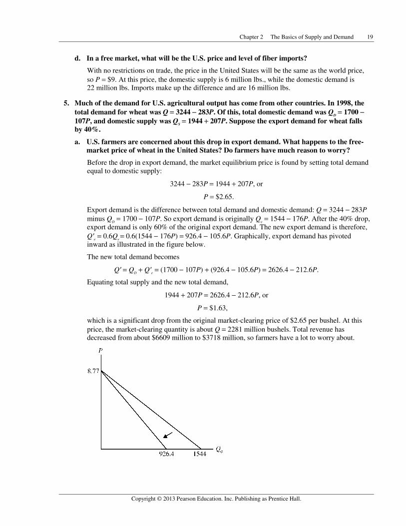
Export demand is the difference between total demand and domestic demand: Q = 3244 − 283P minus QD = 1700 − 107P. So export demand is originally Qe = 1544 − 176P. After the 40% drop, export demand is only 60% of the original export demand. The new export demand is therefore, Q′e = 0.6Qe = 0.6(1544 − 176P) = 926.4 − 105.6P. Graphically, export demand has pivoted inward as illustrated in the figure below.

The new total demand becomes

Q′ = QD + Q′e = (1700 − 107P) + (926.4 − 105.6P) = 2626.4 − 212.6P.

Equating total supply and the new total demand,

1944 + 207P = 2626.4 − 212.6P, or

P = $1.63,

which is a significant drop from the original market-clearing price of $2.65 per bushel. At this price, the market-clearing quantity is about Q = 2281 million bushels. Total revenue has decreased from about $6609 million to $3718 million, so farmers have a lot to worry about.



b. Now suppose the U.S. government wants to buy enough wheat to raise the price to $3.50 per bushel. With the drop in export demand, how much wheat would the government have to buy? How much would this cost the government?

With a price of $3.50, the market is not in equilibrium. Quantity demanded and supplied are

Q′ = 2626.4 − 212.6(3.50) = 1882.3, and

QS = 1944 + 207(3.50) = 2668.5.

Excess supply is therefore 2668.5 − 1882.3 = 786.2 million bushels. The government must purchase this amount to support a price of $3.50, and will have to spend $3.50(786.2 million) = $2751.7 million.

6. The rent control agency of New York City has found that aggregate demand is QD = 160 − 8P. Quantity is measured in tens of thousands of apartments. Price, the average monthly rental rate, is measured in hundreds of dollars. The agency also noted that the increase in Q at lower P results from more three-person families coming into the city from Long Island and demanding apartments. The city’s board of realtors acknowledges that this is a good demand estimate and has shown that supply is QS = 70 + 7P.

a. If both the agency and the board are right about demand and supply, what is the free-market price? What is the change in city population if the agency sets a maximum average monthly rent of $300 and all those who cannot find an apartment leave the city?

Set supply equal to demand to find the free-market price for apartments:

160 − 8P = 70 + 7P, or P = 6,

which means the rental price is $600 since price is measured in hundreds of dollars. Substituting the equilibrium price into either the demand or supply equation to determine the equilibrium quantity:

QD = 160 − 8(6) = 112

and

QS = 70 + 7(6) = 112.

The quantity of apartments rented is 1,120,000 since Q is measured in tens of thousands of apartments. If the rent control agency sets the rental rate at $300, the quantity supplied would be 910,000 (QS = 70 + 7(3) = 91), a decrease of 210,000 apartments from the free-market equilibrium. Assuming three people per family per apartment, this would imply a loss in city population of 630,000 people. Note: At the $300 rental rate, the demand for apartments is 1,360,000 units, and the resulting shortage is 450,000 units (1,360,000 − 910,000). However, excess demand (the shortage) and lower quantity demanded are not the same concept. The shortage of 450,000 units is the difference between the number of apartments demanded at the new lower price (including the number demanded by new people who would have moved into the city), and the number supplied at the lower price. But these new people will not actually move into the city because the apartments are not available. Therefore, the city population will fall by 630,000, which is due to the drop in the number of apartments available from 1,120,000 (the old equilibrium value) to 910,000.



b. Suppose the agency bows to the wishes of the board and sets a rental of $900 per month on all apartments to allow landlords a “fair” rate of return. If 50% of any long-run increases in apartment offerings come from new construction, how many apartments are constructed?

At a rental rate of $900, the demand for apartments would be 160 − 8(9) = 88, or 880,000 units, which is 240,000 fewer apartments than the original free-market equilibrium number of 1,120,000. Therefore, no new apartments would be constructed.

7. In 2010, Americans smoked 315 billion cigarettes, or 15.75 billion packs of cigarettes. The average retail price (including taxes) was about $5.00 per pack. Statistical studies have shown that the price elasticity of demand is −0.4, and the price elasticity of supply is 0.5.

a. Using this information, derive linear demand and supply curves for the cigarette market.

Let the demand curve be of the form Q = a − bP and the supply curve be of the form Q = c + dP, where a, b, c, and d are positive constants. To begin, recall the formula for the price elasticity of demand

.DP

P QE

Q P

Δ=Δ

We know the demand elasticity is –0.4, P = 5, and Q = 15.75, which means we can solve for the slope, −b, which is ΔQ/ΔP in the above formula.

50.4

15.7515.75

0.4 1.26 .5

Q

PQ

bP

Δ− =Δ

Δ = − = − = − Δ

To find the constant a, substitute for Q, P, and b in the demand function to get 15.75 = a − 1.26(5), so a = 22.05. The equation for demand is therefore Q = 22.05 − 1.26P. To find the supply curve, recall the formula for the elasticity of supply and follow the same method as above:

50.5

15.7515.75

0.5 1.575 .5

SP

P QE

Q P

Q

PQ

dP

Δ=Δ

Δ=Δ

Δ = = = Δ

To find the constant c, substitute for Q, P, and d in the supply function to get 15.75 = c + 1.575(5) and c = 7.875. The equation for supply is therefore Q = 7.875 + 1.575P.

b. In 1998, Americans smoked 23.5 billion packs cigarettes, and the retail price was about $2.00 per pack. The decline in cigarette consumption from 1998 to 2010 was due in part to greater public awareness of the health hazards from smoking, but was also due in part to the increase in price. Suppose that the entire decline was due to the increase in price. What could you deduce from that about the price elasticity of demand?

Calculate the arc elasticity of demand since we have a range of prices rather than a single price. The arc elasticity formula is

P

Q PE

P Q

Δ=Δ



where P and Q are average price and quantity, respectively. The change in quantity was 15.75 −23.5 = −7.75, and the change in price was 5 − 2 = 3. The average price was (2 + 5)/2 = 3.50, and the average quantity was (23.5 + 15.75)/2 = 19.625. Therefore, the price elasticity of demand, assuming that the entire decline in quantity was due solely to the price increase, was

Δ −= = = −Δ

7.75 3.500.46.

3 19.625P

Q PE

P Q

8. In Example 2.8 we examined the effect of a 20% decline in copper demand on the price of copper, using the linear supply and demand curves developed in Section 2.6. Suppose the long-run price elasticity of copper demand were −0.75 instead of −0.5.

a. Assuming, as before, that the equilibrium price and quantity are P* = $3 per pound and Q* = 18 million metric tons per year, derive the linear demand curve consistent with the smaller elasticity.

Following the method outlined in Section 2.6, solve for a and b in the demand equation QD = a − bP. Because −b is the slope, we can use −b rather than ΔQ/ΔP in the elasticity

formula. Therefore, *

.*D

PE b

Q

= −

Here ED = −0.75 (the long-run price elasticity), P* = 3

and Q* = 18. Solving for b,

30.75 ,

18b − = −

or b = 0.75(6) = 4.5.

To find the intercept, we substitute for b, QD (= Q*), and P (= P*) in the demand equation:

18 = a − 4.5(3), or a = 31.5.

The linear demand equation is therefore

QD = 31.5 − 4.5P.

b. Using this demand curve, recalculate the effect of a 20% decline in copper demand on the price of copper.

The new demand is 20% below the original (using our convention that quantity demanded is reduced by 20% at every price); therefore, multiply demand by 0.8 because the new demand is 80% of the original demand:

(0.8)(31.5 4.5 ) 25.2 3.6 .DQ P P′ = − = −

Equating this to supply,

25.2 − 3.6P = −9 + 9P, so P = $2.71.

With the 20% decline in demand, the price of copper falls from $3.00 to $2.71 per pound. The decrease in demand therefore leads to a drop in price of 29 cents per pound, a 9.7% decline.



9. In Example 2.8 (page 52), we discussed the recent increase in world demand for copper, due in part to China’s rising consumption.

a. Using the original elasticities of demand and supply (i.e., ES = 1.5 and ED = −0.5), calculate the effect of a 20% increase in copper demand on the price of copper.

The original demand is Q = 27 − 3P and supply is Q = −9 + 9P as shown on page 51. The 20% increase in demand means that the new demand is 120% of the original demand, so the new demand is Q′D = 1.2Q. Q′D = (1.2)(27 − 3P) = 32.4 − 3.6P. The new equilibrium is where Q′D equals the original supply:

32.4 − 3.6P = −9 + 9P.

The new equilibrium price is P* = $3.29 per pound. An increase in demand of 20%, therefore, entails an increase in price of 29 cents per pound, or 9.7%.

b. Now calculate the effect of this increase in demand on the equilibrium quantity, Q*.

Using the new price of $3.29 in the supply curve, the new equilibrium quantity is Q* = −9 + 9(3.29) = 20.61 million metric tons per year, an increase of 2.61 million metric tons (mmt) per year. Except for rounding, you get the same result by plugging the new price of $3.29 into the new demand curve. So an increase in demand of 20% entails an increase in quantity of 2.61 mmt per year, or 14.5%.

c. As we discussed in Example 2.8, the U.S. production of copper declined between 2000 and 2003. Calculate the effect on the equilibrium price and quantity of both a 20% increase in copper demand (as you just did in part a) and of a 20% decline in copper supply.

The new supply of copper falls (shifts to the left) to 80% of the original, so Q′S = 0.8Q = (0.8)(−9 + 9P) = −7.2 + 7.2P. The new equilibrium is where Q′D = Q′S.

32.4 − 3.6P = −7.2 + 7.2P

The new equilibrium price is P* = $3.67 per pound. Plugging this price into the new supply equation, the new equilibrium quantity is Q* = −7.2 + 7.2(3.67) = 19.22 million metric tons per year. Except for rounding, you get the same result if you substitute the new price into the new demand equation. The combined effect of a 20% increase in demand and a 20% decrease in supply is that price increases by 67 cents per pound, or 22%, and quantity increases by 1.22 mmt per year, or 6.8%, compared to the original equilibrium.

10. Example 2.9 (page 54) analyzes the world oil market. Using the data given in that example:

a. Show that the short-run demand and competitive supply curves are indeed given by

D = 33.6 − 0.020P

SC = 18.05 + 0.012P.

The competitive (non-OPEC) quantity supplied is Sc = Q* = 19. The general form for the linear competitive supply equation is SC = c + dP. We can write the short-run supply elasticity as ES = d(P*/Q*). Since ES = 0.05, P* = $80, and Q* = 19, 0.05 = d(80/19). Hence d = 0.011875. Substituting for d, Sc, and P in the supply equation, c = 18.05, and the short-run competitive supply equation is Sc = 18.05 + 0.012P.



Similarly, world demand is D = a − bP, and the short-run demand elasticity is ED = −b(P*/Q*), where Q* is total world demand of 32. Therefore, −0.05 = −b(80/32), and b = 0.020. Substituting b = 0.02, D = 32, and P = 80 in the demand equation gives 32 = a − 0.02(80), so that a = 33.6. Hence the short-run world demand equation is D = 33.6 − 0.020P.

b. Show that the long-run demand and competitive supply curves are indeed given by

D = 41.6 − 0.120P

SC = 13.3 + 0.071P.

Do the same calculations as above but now using the long-run elasticities, ES = 0.30 and ED = −0.30: ES = d(P*/Q*) and ED = −b(P*/Q*), implying 0.30 = d(80/19) and −0.30 = −b(80/32). So d = 0.07125 and b = 0.12.

Next solve for c and a: Sc = c + dP and D = a − bP, implying 19 = c + 0.07125(80) and 32 = a − 0.12(80). So c = 13.3 and a = 41.6.

c. In Example 2.9 we examined the impact on price of a disruption of oil from Saudi Arabia. Suppose that instead of a decline in supply, OPEC production increases by 2 billion barrels per year (bb/yr) because the Saudis open large new oil fields. Calculate the effect of this increase in production on the supply of oil in both the short run and the long run.

OPEC’s supply increases from 13 bb/yr to 15 bb/yr as a result. Add 15 bb/yr to the short-run and long-run competitive supply equations. The new total supply equations are:

Short-run: ST′ = 15 + Sc = 15 + 18.05 + 0.012P = 33.05 + 0.012P, and

Long-run: ST″ = 15 + Sc = 15 + 13.3 + 0.071P = 28.3 + 0.071P.

These are equated with short-run and long-run demand, so that:

33.05 + 0.012P = 33.6 − 0.020P, implying that P = $17.19 in the short run, and

28.3 + 0.071P = 41.6 − 0.120P, implying that P = $69.63 in the long run.

In the short run, total supply is 33.05 + 0.012(17.19) = 33.26 bb/yr. In the long run, total supply remains virtually the same at 28.3 + 0.071(69.63) = 33.24 bb/yr. Compared to current total supply of 32 bb/yr, supply increases by about 1.25 bb/yr.

11. Refer to Example 2.10 (page 59), which analyzes the effects of price controls on natural gas.

a. Using the data in the example, show that the following supply and demand curves describe the market for natural gas in 2005–2007:

Supply: Q = 15.90 + 0.72PG + 0.05PO

Demand: Q = 0.02 − 1.8PG + 0.69PO

Also, verify that if the price of oil is $50, these curves imply a free-market price of $6.40 for natural gas.

To solve this problem, apply the analysis of Section 2.6 using the definition of cross-price elasticity of demand given in Section 2.4. For example, the cross-price elasticity of demand for natural gas with respect to the price of oil is:

.G OGO

O G

Q PE

P Q

Δ= Δ



G

O

Q

P

Δ Δ

is the change in the quantity of natural gas demanded because of a small change in

the price of oil, and for linear demand equations, it is constant. If we represent demand as

–G G OQ a bP eP= + (notice that income is held constant), then .G

O

Qe

P

Δ= Δ

Substituting this into

the cross-price elasticity, *

*,O

GOG

PE e

Q

=

where *

OP and *GQ are the equilibrium price and quantity.

We know that * $50oP = and * 23GQ = trillion cubic feet (Tcf). Solving for e,

501.5 ,

23e =

or e = 0.69.

Similarly, representing the supply equation as ,G G OQ c dP gP= + + the cross-price elasticity of

supply is *

*,O

G

Pg

Q

which we know to be 0.1. Solving for g,

=23

501.0 g , or g = 0.5 rounded to

one decimal place.

We know that ES = 0.2, PG* = 6.40, and Q* = 23. Therefore,

=

23

40.62.0 d , or d = 0.72. Also,

ED = −0.5, so

−=−

23

40.65.0 b , and thus b = 1.8.

By substituting these values for d, g, b, and e into our linear supply and demand equations, we may solve for c and a:

23 = c + 0.72(6.40) + 0.05(50), so c = 15.9, and

23 = a − 1.8(6.40) + 0.69(50), so that a = 0.02.

Therefore, the supply and demand curves for natural gas are as given. If the price of oil is $50, these curves imply a free-market price of $6.40 for natural gas as shown below. Substitute the price of oil in the supply and demand equations. Then set supply equal to demand and solve for the price of gas.

15.9 + 0.72PG + 0.05(50) = 0.02 − 1.8PG + 0.69(50)

18.4 + 0.72PG = 34.52 − 1.8PG

PG = $6.40.

b. Suppose the regulated price of gas were $4.50 per thousand cubic feet instead of $3.00. How much excess demand would there have been?

With a regulated price of $4.50 for natural gas and the price of oil equal to $50 per barrel,

Demand: QD = 0.02 − 1.8(4.50) + 0.69(50) = 26.4, and

Supply: QS = 15.9 + 0.72(4.50) + 0.05(50) = 21.6

With a demand of 26.4 Tcf and a supply of 21.6 Tcf, there would be an excess demand (i.e., a shortage) of 4.8 Tcf.



c. Suppose that the market for natural gas remained unregulated. If the price of oil had increased from $50 to $100, what would have happened to the free-market price of natural gas?

In this case

Demand: QD = 0.02 − 1.8PG + 0.69(100) = 69.02 − 1.8PG, and

Supply: QS = 15.9 + 0.72PG + 0.05(100) = 20.9 + 0.72PG.

Equating supply and demand and solving for the equilibrium price,

20.9 + 0.72PG = 69.02 – 1.8PG, or PG = $19.10.

The free-market price of natural gas would have almost tripled from $6.40 to $19.10.

12. The table below shows the retail price and sales for instant coffee and roasted coffee for two years.

Year

Retail Price of Instant Coffee

($/Lb)

Sales of Instant Coffee

(Million Lbs)

Retail Price of Roasted Coffee

($/Lb)

Sales of Roasted Coffee (Million Lbs)

Year 1 10.35 75 4.11 820

Year 2 10.48 70 3.76 850

a. Using these data alone, estimate the short-run price elasticity of demand for roasted coffee. Derive a linear demand curve for roasted coffee.

To find elasticity, first estimate the slope of the demand curve:

820 850 3085.7

4.11 3.76 0.35

Q

P

Δ − −= = = −Δ −

Given the slope, we can now estimate elasticity using the price and quantity data from the above table. Assuming the demand curve is linear, the elasticity will differ the two years because price and quantity are different. We can calculate the elasticities at both points and also find the arc elasticity at the average point between the two years:

Δ= = − = −ΔΔ= = − = −ΔΔ= = − = −Δ

1

2

4.11( 85.7) 0.043

820

3.76( 85.7) 0.038

850

3.935( 85.7) 0.040.

835

P

P

ARCP

P QE

Q P

P QE

Q P

P QE

Q P

To derive the demand curve for roasted coffee, Q = a − bP, note that the slope of the demand curve is −85.7 = −b. To find the coefficient a, use either of the data points from the table above so that 820 = a − 85.7(4.11) or 850 = a − 85.7(3.76). In either case, a = 1172.2. The equation for the demand curve is therefore

Q = 1172.2 − 85.7P.



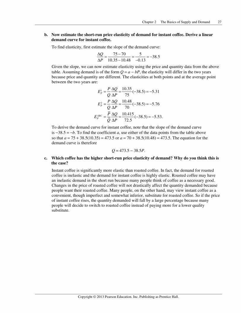
b. Now estimate the short-run price elasticity of demand for instant coffee. Derive a linear demand curve for instant coffee.

To find elasticity, first estimate the slope of the demand curve:

75 70 538.5

10.35 10.48 0.13

Q

P

Δ −= = = −Δ − −

Given the slope, we can now estimate elasticity using the price and quantity data from the above table. Assuming demand is of the form Q = a − bP, the elasticity will differ in the two years because price and quantity are different. The elasticities at both points and at the average point between the two years are:

1

2

10.35( 38.5) 5.31

75

10.48( 38.5) 5.76

70

10.415( 38.5) 5.53.

72.5

P

P

ARCP

P QE

Q P

P QE

Q P

P QE

Q P

Δ= = − = −ΔΔ= = − = −ΔΔ= = − = −Δ

To derive the demand curve for instant coffee, note that the slope of the demand curve is −38.5 = −b. To find the coefficient a, use either of the data points from the table above so that a = 75 + 38.5(10.35) = 473.5 or a = 70 + 38.5(10.48) = 473.5. The equation for the demand curve is therefore

Q = 473.5 − 38.5P.

c. Which coffee has the higher short-run price elasticity of demand? Why do you think this is the case?

Instant coffee is significantly more elastic than roasted coffee. In fact, the demand for roasted coffee is inelastic and the demand for instant coffee is highly elastic. Roasted coffee may have an inelastic demand in the short run because many people think of coffee as a necessary good. Changes in the price of roasted coffee will not drastically affect the quantity demanded because people want their roasted coffee. Many people, on the other hand, may view instant coffee as a convenient, though imperfect and somewhat inferior, substitute for roasted coffee. So if the price of instant coffee rises, the quantity demanded will fall by a large percentage because many people will decide to switch to roasted coffee instead of paying more for a lower quality substitute.

Microeconomics 8th Edition Pindyck Solutions ManualFull Download: http://testbanklive.com/download/microeconomics-8th-edition-pindyck-solutions-manual/

Full download all chapters instantly please go to Solutions Manual, Test Bank site: testbanklive.com

http://testbanklive.com/download/microeconomics-8th-edition-pindyck-solutions-manual/

Documents

Chapter 2 - testbanklive.com · Microeconomics 8th Edition Pindyck Solutions Manual Full Download: