3.1

Chapter 3Entering Data into CrimeStat

Th e gr aphic u ser in ter face of Crim eS tat is a t abbed form (figure 3.1). Ther e a re fivegroups of funct ions : Da ta setup , Spa t ia l descr ip t ion , Spa t ia l modeling, Cr ime TravelDemand, an d Opt ions. Ea ch group, in t u rn is made up of severa l set s of rou t ines :

D a ta Se t up

Pr imary file Da ta file of inciden t /poin t loca t ions (Required)Seconda ry file Secondary da ta file of in ciden t /poin t loca t ion sReferen ce file File for referencin g in terpola t ion sMeasuremen t Pa rameter s Area l and linea r cha ract er is t ics of s tudy a rea

Spat ia l Descr iption

Spat ia l Dis t r ibu t ion Basic ch aracter is t ics of the in ciden t dis t r ibu t ionDista nce Ana lysis I Character ist ics of th e dist ances bet ween point sDista nce Ana lysis II Mat r ix dist ances‘Hot Spot’ Ana lysis I Tools for iden t ifyin g ‘Hot Spots’‘Hot Spot’ Ana lysis II More tools for identifying ‘Hot Spots’

S pa ti al Mo de li ng

In ter pola t ion Three-dim en siona l den sit y ana lysisJ our ney-to-cr ime Ana lysis Analyzing th e t r avel beha vior of ser ial offender sSpace-t ime Ana lysis The in ter action bet ween space an d t ime

Cri m e Tra ve l D e m a nd

Tr ip genera t ion Models of cr im e or igin s and cr im e dest in a t ion sTr ip dis t r ibu t ion Model of t r ips between or igin s and dest in a t ion sMode split Model of t r avel mode used for t r ipsNetwork ass ignment Model of rout e t aken for t r ipsFile worksheet Worksheet of file names

Op ti on s

Save parameter s Save the dat a setup parameter sLoad parameter s Load a lrea dy-sa ved paramet er s fileColor s Change th e color of t absSim ula t ion Outpu t simu la t ion da t a

This section discusses th e Data Setup t abs.

CrimeStat User InterfaceFigure 3.1:

3.3

Requ ired Data

Crim eS tat can input dat a in several form at s - ASCII, dbase III/ IV ‘dbf’, ArcView‘sh p’, MapIn fo ‘dat ’, an d files tha t su pport th e ODBC sta nda rd, such a s Excel®, Lotus 1-2-3®, Microsoft Access®, and Paradox®. It is ess en t ial t ha t the files ha ve X and Y coordina tesas pa r t of their s t ructure. The pr ogra m assu mes t ha t the assigned X and Y coordina tesa re cor rect . It rea ds a file - ASCII, ‘dbf’ or ‘sh p’ and t akes the given X and Y coordin a tes .

If you r ead an ArcView sh ape file, the inciden t ’s X and Y coordina tes a reau toma t ically a dded as t he first fields in the pr imary file by Crim eS tat. If you use a nyoth er type of file you m ust add X an d Y coordina tes to the file. To au toma te th is in

ArcView , a dd the Avenue ext ension Coord in ate Utili ty V1.0 (ava ilable in Arc Scr ip t s) toyour exten sion list . To do th is in MapIn fo add the KGM u t ility Table Geography a s a t ool. Both work grea t . It is a good idea to add t he X an d Y coordin a tes to an y file. They a reusefu l for ana lysis in other progr ams and a llow for easy r econst ruct ion of the file if t he geo-codin g is lost .

Co ord in a te s

Crim eS tat ana lyzes poin t da ta , defined geogra ph ically by X and Y coordin a tes . Th ese X/Y coord ina tes represen t a sin gle loca t ion wher e eit her an inciden t occur red (e.g., abu rglary) or wh er e a bu ildin g or oth er object can be r epresen ted as a sin gle point . A pointwill have X and Y coordina tes in a spher ica l or Ca r t es ian sys t em. In a spher ica l coordina tesys tem, each poin t can be defin ed by longitude (for X) and la t it ude (for Y). In a projectedcoordina te syst em, such a s St a te Pla ne or UTM, each X and Y is defined by feet or metersfrom an arbit ra ry refer en ce or igin . Crim eS tat can handle both sph er ica l an d pr ojectedpoint s. F or some uses, coord ina tes can be pola r , tha t is defined a s a ngles from a n arbit ra ryreference vector , u sua lly d ir ect nor th .1 One of th e rout ines in t he progra m calculat es theangula r mea n and va r iance of a collect ion of an gles .

Point da ta can be obta ined from a number of sour ces. The m ost frequent would bethe va r iou s in ciden t da ta bases stored by a police depar tment , which could in clu de ca lls forservice, crim e r eport s, or closed cases. Other sources of inciden t da ta can includesecondary da ta from other agencies (e.g., hospit a l r ecords, emergency m edica l servicerecords , loca t ions of bu sin esses) or even sa mpled da ta (Levine a nd Wa chs , 1986a ; 1986b). There a re a lso poin t da ta from broadcast sources, such as radios , t elevision s, ormicrowaves.

To read projected coordin a tes in to Crim eS tat, th e user doesn’t need t o define thepa r t icula r pr oject ion (oth er than to ind icat e t ha t the coord ina tes a re projected). ArcViewwill ou tpu t the object s in the p rojected un it s so tha t they can be read direct ly in to tha tp rogram or in to ArcGIS . H owever , t o outpu t ca lcu la ted object s to MapIn fo r equ ires thedefin ition of the specific pr oject ion used.2 See cha pt er 4 for the firs t examples of out pu t ingobjects.

3.4

Inten sit ies and w eig hts

For some uses, poin t s can have intensity va lu es or weights . These a re opt ion a linpu ts in Crim eS tat. An intensity is a va lu e assigned to a poin t loca t ion aside from theX/Y coordin a tes. It is another va r ia ble, t ypica lly denoted as a Z-va lu e. F or example, if thepoin t loca t ion is the loca t ion of a police st a t ion , t hen the in tensit y cou ld be the number ofca lls for service over a mon th a t tha t st a t ion . Or , t o u se census geography, if t he poin t isthe cen t roid of a censu s t r act , th en the int ensity could be th e popula t ion of tha t censu st ract . In other words, a n in tensit y is a va r ia ble assigned to a par t icu la r loca t ion .

Some of the rou t ines in Crim eS tat r equ ire an in ten sit y value (e.g., the spa t ia lau tocorr ela t ion indices) and other s can u t ilize a point locat ion wit h an in ten sit y valueassigned (e.g., kernel dens ity int erpola t ion). If no int ensity va lue is a ssigned, th e rou t ineswhich require it cannot be ru n while the rou t ines which can u t ilize it will assu me tha t thein tensit y is 1 (i.e., tha t a ll poin t s have equa l in tensit y).

A weigh t occurs when differen t poin t loca t ion s a re to receive differen t ia l s t a t is t ica lt r ea tment . For exam ple, if a police depa r tment has des igna ted differen t a reas for ser vice,for exa mple ‘urban’ and ‘rura l’, a va lu e can be assigned for each of these a reas (e.g., ‘1' forurba n and ‘2' for ru ra l). Most of the r out ines in Crim eS tat will use the weight s in theca lcu la t ion s. Weight s would be usefu l if differen t zon es a re to be eva lu a ted on the basis ofanother var iable. For exam ple, suppose a police depa r tment has divided its ser vice areain to u rban and ru ra l. In the ru ra l pa r t , there a re twice as many pa t rol officer s ass ignedper capita th an in t he ur ban a reas; the higher populat ion densities in t he ur ban a reas a reassu med to compensa te for t he longer tr avel dista nces in t he ru ra l ar eas. Let’s assu metha t a ll cr imes occur r ing in t he rura l ar eas r eceive a weight of 2 while those in the urbanarea receive a weight of 1. Th e police depar tment then wants to est im ate the densit y ofhouseh old bur gla r ies relat ive to the popula t ion using th e du el ker nel dens ity funct ion (seeCh apt er 7). But , to reflect t he differ en t ia l ass ignmen t of police officers, t he a na lyst s u sethe ser vice a rea as a weigh t . The r esu lt would be a per capita est imate of bu rglary den sit y(i.e., bu rglar ies per person), bu t weigh ted by the ser vice a rea . It would pr ovide an est imateof burglar y risk adjusted for different ial service in r ur al an d ur ban a reas. In most cases,ther e will n o weigh t s, in wh ich case , a ll poin t s a re a ssumed to ha ve a n equ a l weigh t of ‘1'.

It is possible to have both in tensit ies and weight s, a lt hough th is would be ra re. F orexample, if the X and Y coord ina tes a re the cen t roids of census t r act s , a th ird va r iable - the tota l popu lat ion of each censu s t r act cou ld be an int ensity. Ther e could a lso be anweight ing ba sed on service area . In calcu la t ing the Moran’s I spa t ia l au tocorr ela t ion in dex,th e tota l populat ion is used a s an inten sity while th e service ar ea is used as a weight. Inth is case , Crim eS tat ca lcu la tes a weighted Moran’s I spa t ia l a u tocorrela t ion .

Bu t t he use of both an in t ensity and a weight would be less common. F or most ofth e stat istics, a variable could be used as either a weigh t or a n in ten sit y, and t he r esu lt swill be t he same. However , be car eful in ass igning the same var iable a s both an in ten sit yand a weigh t . In su ch in st ances, cases may end u p being weigh ted twice, which willproduce distort ed results.3

3.5

Ti m e Me a su re s

Crim eS tat now in clu des rout in es for ana lyzing spa t ia l ch aracter is t ics in rela t ion tot im e. Many ser ia l cr im e in ciden t s occur in a shor t per iod of t im e. F or exa mple, a gr oup ofcar th ieves may s tea l ca r s from a neighborhood over a very shor t per iod of t im e, forexample a few da ys. Th us, t her e is often an in ter action bet ween a concent ra ted spa t ia lpa t t ern of event s occur r ing in a sh or t t ime per iod. Because of th is, police depa r tmentsrou t ine collect informat ion on the t ime of the event , th e da y an d t ime.

Th ere a re th ree rout in es which ana lyze spa t ia l concen t ra t ion in rela t ion to t im e: theKnox index, th e Mantel index, an d a cor relat ed wa lk m odel. But for using an y of theserout ines , the u ser has t o define t ime in a consis t en t manner . Both the pr imary andseconda ry files can a llow a t ime va r iable. H owever , these have to be defined in a consisten tma nn er for a ll records in a file. There are five time periods th at ar e allowed:

HourDay (defau lt )WeekMonthYear

The defau lt is ‘da y’. Tha t is, t he program will assume t ha t any t ime va r iable is inda ys, either an a rbit ra ry number of da ys (e.g., days from J anuary 1s t) or t he number ofda ys from J anuary 1, 1900, wh ich is the defau lt t ime r efer en ce for m ost compu ter sys tem s. If the t ime un it is n ot in da ys, t he u ser needs t o indicate t he appropr ia te un it .

Miss ing Value Codes

Unfor tuna tely, da ta is frequ en t ly messy. In most police depar tmen ts, t he crim ein ciden t da ta base is bein g con t in ua lly u pda ted, da ily a nd, perhaps, h our ly. At any on et ime, many of th e r ecords will not h ave been geocoded or will have been incompletelygeocoded.

B la n k r e cor d s

Crim eS tat a llows the inclus ion of codes for miss ing values, tha t is va lues of eligiblefields tha t a re not complete or a re not cor rect . These codes a re applied t o the fields definedon t he pr imary or seconda ry da ta set s (X, Y, weigh t , in ten sit y). Aut oma t ically, Crim eS tatwill exclude records wit h bla nk fields or with fields having any non-numer ic valu e (e.g.,a lph anumer ic cha racter s, #, *) for the eligible fields . The st a t ist ics will be calcula ted onlyon t hose r ecords wh ich h ave eligible n umer ical va lues. Fields for oth er var iables in thedat a base th at ar e not defined in t he prima ry and seconda ry data sets will be ignored.

3.6

Ot h er m iss in g v a lu e cod es

In add it ion t o blank and n on-numer ic valu es , Crim eS tat can exclude any otherva lue t ha t has been used for a miss ing values code (e.g., 0, -1, 99). Tha t is, if the progra mencounter s a field wit h a missin g va lu e code, it will exclude tha t record from theca lcu la t ions . Next to the X, Y, weigh t and in tens ity fields on both the p r imary andseconda ry files is a miss ing values code box. The defau lt has been set to blan k. Tha t is, ifCrim eS tat finds n o informat ion in a field, it will ignore t ha t record. However, th ere areeight options t ha t can be selected:

1. <bl a nk > fields a re au toma t ically excluded. This is the defau lt ;2. <non e> indicates tha t no records will be excluded. If th er e is a blank field,

Crim eS tat will t r ea t it a s a 0;3. 0 is excluded;4. -1 is excluded;5. 0 a n d -1 indicat es tha t both 0 and -1 will be excluded;6. 0, -1 a n d 9999 indica tes t ha t a ll th ree values (0, -1, 9999) will be excluded;7. An y other numer ica l va lue can be t rea ted as a missing va lue by typ ing it

(e.g., 99); and8. Mul t ip l e numer ica l va lues can be tr ea ted a s m issing va lues by typing t hem,

separa t in g each by commas (e.g., 0, -1, 99, 9999, -99).

It is im por tan t for user s t o un derst and t heir da ta set s p r ior t o us ing Crim eS tat. Ifthe da ta a re ‘clean ’, tha t is a ll X/Y fields a re popula ted wit h cor rect values as a re a llweight /int en sit y fields (if used), then the progra m will h ave n o problems r unning rout ines . On the other hand, in la rge adm inist ra t ive da ta bases, su ch as in most police depa r tments,ther e will be m any records tha t a re in complete or have m iss ing values codes (e.g., 0). Un less Crim eS tat is told what a re the missin g va lu e codes, wit h the except ion of blank ornon-numer ic values, it will include them in t he ca lcu lat ions. For example, some da ta basepr ogra ms pu t a 0 for an X or Y field wh ich h as n ot been geocoded. Crim eS tat doesn’t knowtha t the 0 is a missin g va lu e and will u se it in ca lcu la t ion s sin ce 0 is a per fect ly goodnumber . It is im por tan t tha t user s either clea n their da ta thoroughly or define t he m iss ingvalue codes completely for the pr ima ry an d seconda ry files.

P rim ary Fi le

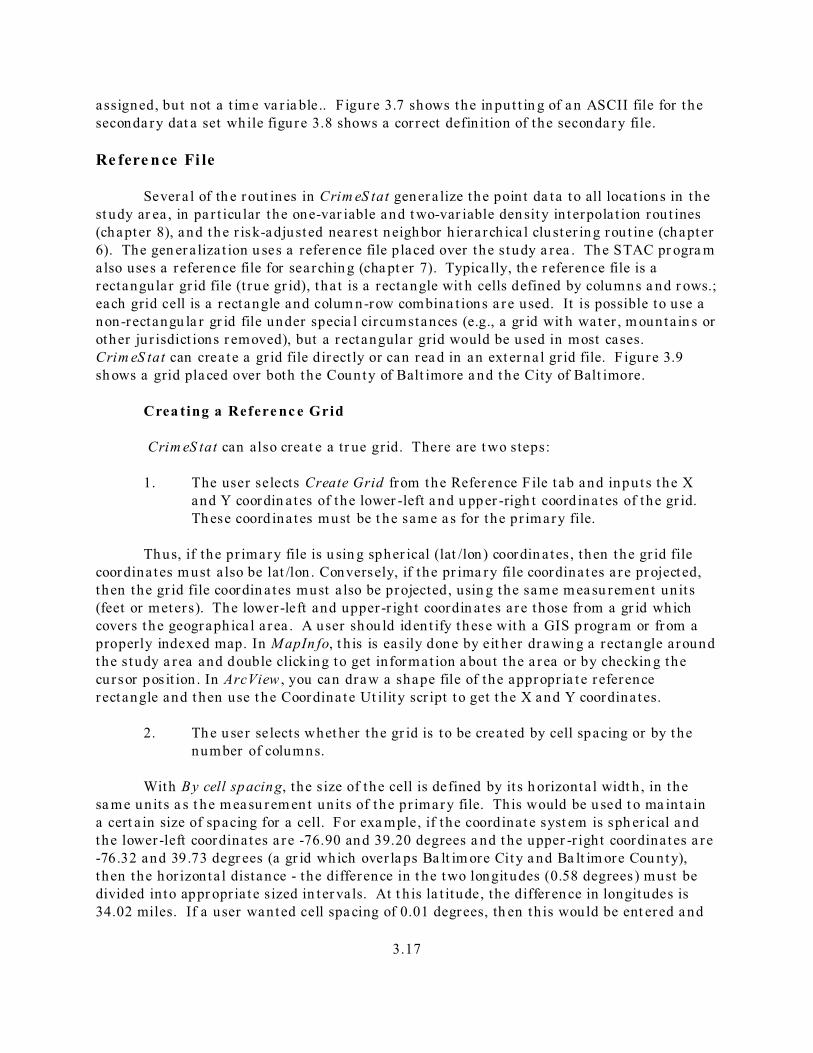
The Prim ary File is r equ ired and p rovides the coord ina tes of poin t s of inciden t s. Onthe pr im ary file t ab, t he user must fir st click on S elect Files. A d ia log box appears tha ta llows t he u ser to select wh ich of six file form ats a pp lies to th e pr imary file (F igure 3.2). For ea ch of the file form ats, t he u ser must define t wo character ist ics - the t ype of file(ASCII, ‘.dbf’, ‘da t ’, ‘.shp’, ‘mdb’, or ODBC) and the name of the file. There is a browsewin dow which a llows t he u ser to find t he file.

In developin g t h is progr am, we have ta rgeted it towards users of ArcView , MapIn foan d Atlas*GIS . These GIS programs either st ore t heir a t t r ibu te da ta in dB ase III/ IVformat in a file wit h a ‘dbf’ extension (e.g., precin ct1.dbf) or can read and wr it e dir ect ly ‘dbf’

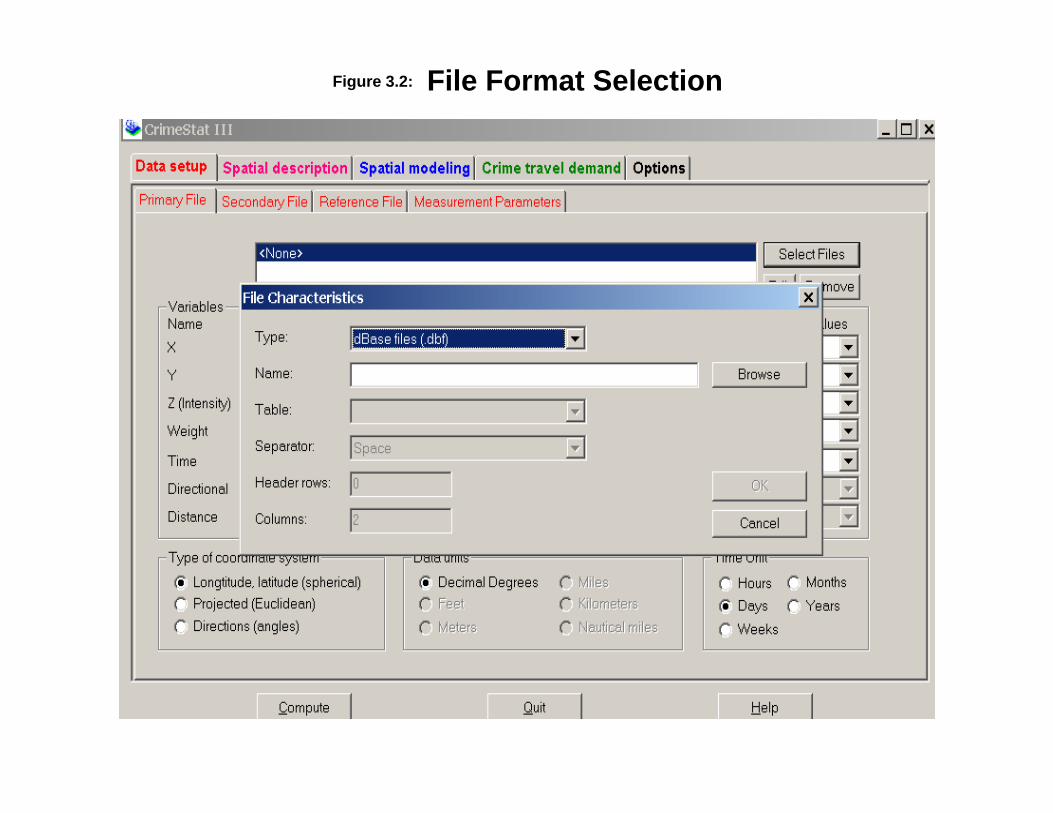
File Format SelectionFigure 3.2:

Linking CrimeStat III to MapInfo

Richard Block Professor of Sociology and Criminal Justice

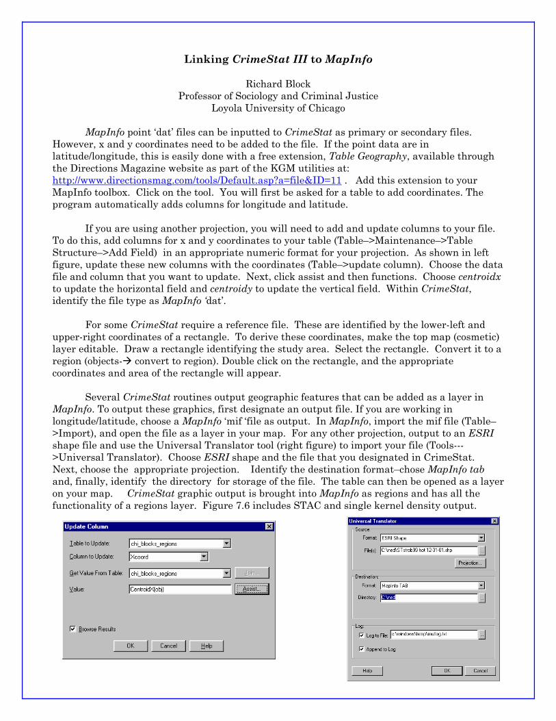
Loyola University of Chicago MapInfo point ‘dat’ files can be inputted to CrimeStat as primary or secondary files. However, x and y coordinates need to be added to the file. If the point data are in latitude/longitude, this is easily done with a free extension, Table Geography, available through the Directions Magazine website as part of the KGM utilities at: http://www.directionsmag.com/tools/Default.asp?a=file&ID=11 . Add this extension to your MapInfo toolbox. Click on the tool. You will first be asked for a table to add coordinates. The program automatically adds columns for longitude and latitude.

If you are using another projection, you will need to add and update columns to your file. To do this, add columns for x and y coordinates to your table (Table–>Maintenance–>Table Structure–>Add Field) in an appropriate numeric format for your projection. As shown in left figure, update these new columns with the coordinates (Table–>update column). Choose the data file and column that you want to update. Next, click assist and then functions. Choose centroidx to update the horizontal field and centroidy to update the vertical field. Within CrimeStat, identify the file type as MapInfo ‘dat’.

For some CrimeStat require a reference file. These are identified by the lower-left and upper-right coordinates of a rectangle. To derive these coordinates, make the top map (cosmetic) layer editable. Draw a rectangle identifying the study area. Select the rectangle. Convert it to a region (objects- convert to region). Double click on the rectangle, and the appropriate coordinates and area of the rectangle will appear.

Several CrimeStat routines output geographic features that can be added as a layer in MapInfo. To output these graphics, first designate an output file. If you are working in longitude/latitude, choose a MapInfo ‘mif ‘file as output. In MapInfo, import the mif file (Table–>Import), and open the file as a layer in your map. For any other projection, output to an ESRI shape file and use the Universal Translator tool (right figure) to import your file (Tools--->Universal Translator). Choose ESRI shape and the file that you designated in CrimeStat. Next, choose the appropriate projection. Identify the destination format–chose MapInfo tab and, finally, identify the directory for storage of the file. The table can then be opened as a layer on your map. CrimeStat graphic output is brought into MapInfo as regions and has all the functionality of a regions layer. Figure 7.6 includes STAC and single kernel density output.

3.9

files. Many ot her GIS progr ams, h owever , a lso can read ‘dbf’ files. F or ArcView andMapIn fo, the X an d Y coordin a tes wh ich define cr ime in ciden t poin t s a re n ot d irect ly pa r tof the ‘dbf’ file, but ins tead exist on t he geogra ph ic file.

Input Fi le Forma ts

ArcView

In ArcView the coord ina tes a re s tored on the ‘sh p’ file, not t he ‘dbf’ file. Crim eS tatcan rea d d irect ly a ‘sh p’ file so the ‘dbf’ file is n ot r equ ired to ha ve t he X an d Y coordin a tes .

Ma pIn fo

However , in MapIn fo, th e coordina tes ar e stored in ‘ta b’ files. To use Crim eS tatwit h MapIn fo, ther efore, r equ ires tha t the X and Y coordin a tes be a ss igned to two fields inthe ‘t ab’ file and t hen sa ved a s a ‘dbf’ file. See the en dn otes for dir ections on doing th is.4 Even in ArcView , some user s m ay wish t o expor t the poin t s a s a ‘dbf’ file because of otherinform at ion t ha t a re on t he records. The endnotes also list th ese directions.5 MapIn fo alsouses a ‘da t ’ format , wh ich is sim ila r to ‘dbf’. Th is can be r ea dy by Crim eS tat.

Atla s*GIS

In Atlas*GIS , on t he other hand, a poin t file is a lrea dy a ‘dbf’ file and will havefields for the X and Y coordina tes.

Microsoft Access

‘Mdb’ Files from Microsoft Access® 97 (or ea r lier ) can a lso be r ea d by Crim eS tat. The user will have to ensu re tha t the file has a n X and Y coordina te.

ODBC

Sim ila r ly, Crim eS tat can rea d a ny file tha t uses Open Da taba se Conn ectivity(ODBC). ODBC is a pr ogramming inter face tha t enables pr ograms t o access da ta indat abase m an agement systems t ha t u se Stru ctu red Query Lan gua ge (SQL) as a dat aaccess s t anda rd, such as E xcel®, Pa radox®, Micr osoft Access, Lotus 1-2-3®, and FoxPro®.

ASCII

For a n ASCII file, however , th ree a dd it iona l a t t r ibu tes must be defined. Th e firs t isthe type of character tha t is used to separa te the va r ia bles in the file. There a re fourpossibilities:6

Space (one or more, t he defau lt )CommaSemicolon

3.10

Tab

The second cha racter ist ic is the number of rows wh ich have labels on them (HeaderRows). Some ASCII files will have rows which label the names of the var iables. The u sersh ould indicat e the number if th is is the case oth erwise Crim eS tat will p roduce an er rorcode. The defau lt is 0, th at is th e progra m a ssum es tha t t here ar e no headers u nlessinst ructed other wise. To change th is, t he u ser sh ould inser t the cur sor in the appropr ia tecell, backspa ce to erase the defau lt number and t ype in the cor rect number .

The th ir d character is t ic of a n ASCII file tha t must be defin ed is the number ofvar iables (columns or fields) in the file. With spher ical or pr ojected coord ina tes, ther e willbe at leas t two var iables (th e X and Y coordina te) and t here may be more if other var iablesa re included in the file. However, with direct iona l coordina tes (see below), th ere may beonly one. Crim eS tat assu mes th at th e num ber of column s in t he ASCII file is two un lessinst ructed other wise. Again , the u ser sh ould inser t the cur sor in the appropr ia te cell,ba ckspa ce to erase the defau lt number and t ype in the cor rect number . After definin g thefile type and name, t he user should click on OK .

Ide n tify in g Vari ab le s

After definin g a file, either ‘.dbf’, ASCII , ‘da t ’, or ‘.sh p’, it is n ecessa ry to iden t ify th evar iables. Two var iables a re required and t wo are opt iona l. The r equired var iables a re theX and Y coordina tes . The user shou ld indica t e t he file name tha t con ta ins the coordina tesby click ing on the d rop down menu and h igh ligh t ing the cor rect name. After havingident ified which file conta ins t he X an d Y coordin a tes , it is n ecessa ry to iden t ify th eva r iable name. Click on the d rop down menu under Colum n and h igh ligh t the name of thevar iable for t he X an d Y coordin a tes respectively.7 F igure 3.3 shows a correct defin in g offile and var iable names for the pr ima ry file.

Multiple files can be ent ered on the pr ima ry file t ab. However , on ly one can beu t ilized a t a t ime. In theor y, one can have separa te files con ta in ing the X and Ycoordina tes , t hough in pract ice th is will r a r ely occur .

We ig h t Varia ble

Somet imes , a point loca t ion is weighted. As m ent ioned a bove, weight s a re usedwhen poin t s represen t s a reas and the a reas a re st a t is t ica lly t r ea ted differen t ly. F or mostof the s t a t ist ics, Crim eS tat can weigh t the s t a t ist ics dur ing the calcula t ion (e.g., t heweighted mean cen ter , t he weighted nearest neighbor in dex).

By defau lt , Crim eS tat assigns a weight of 1 t o each poin t . If the user does notdefine a weigh t var iable, t hen the progra m assumes tha t ea ch point has equ a l weigh t (i.e.,1). On the other hand, if there a re weight s, t hen the weight va r ia ble should be defin ed onth e primar y file screen an d its n am e listed.

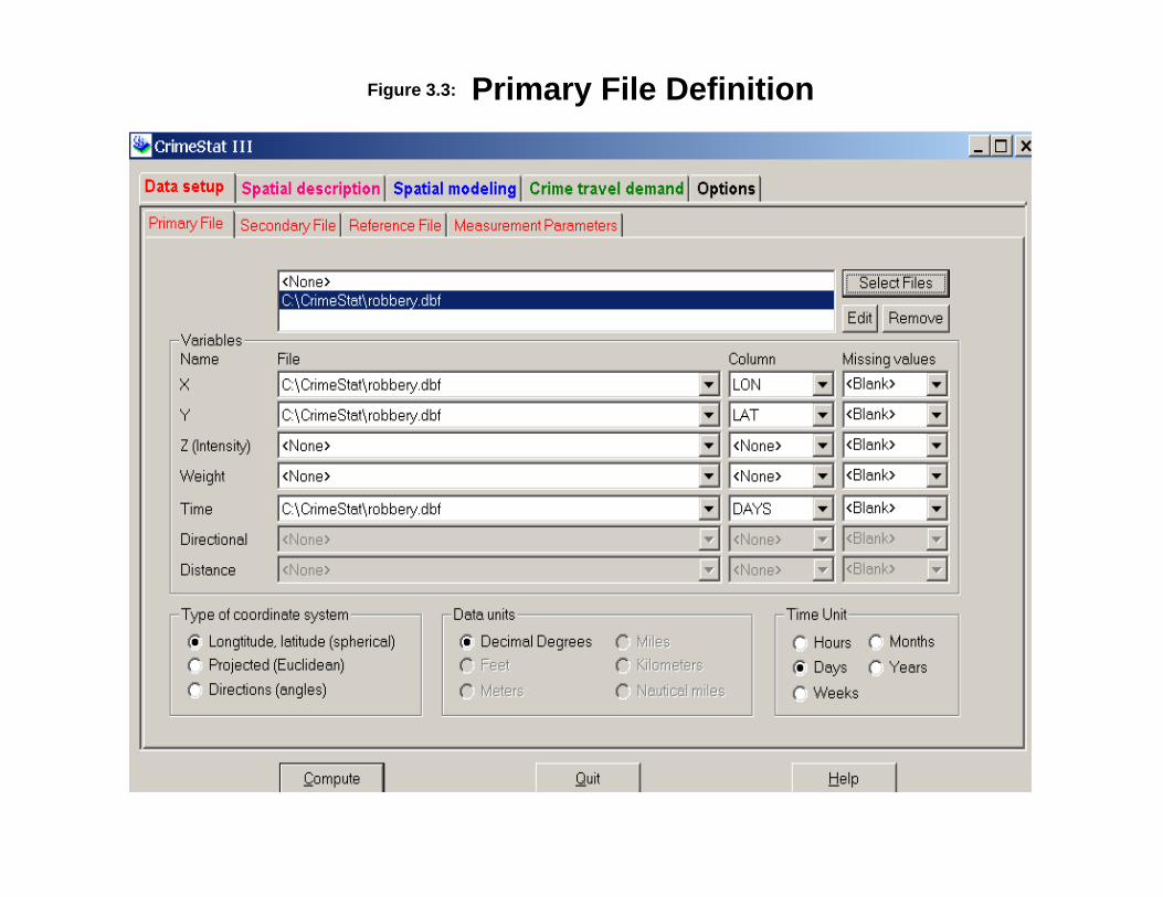
Primary File DefinitionFigure 3.3:

3.12

Int e n si ty Varia ble

Sim ila r ly, a poin t loca t ion can have an in tensit y a ssigned to it . Most of thest a t ist ics in Crim eS tat can use an in tensit y var ia ble and some sta t is t ics requir e it (Moran’sI, Gea ry’s C and Loca l Moran). If no int en sit y is defined, Crim eS tat will not calcula testa t is t ics requir in g a n in tensit y var ia ble and, in st a t is t ics where an in tensit y is opt ion a l(e.g., inter pola t ion), will assume a defau lt in ten sit y of 1. On the oth er hand, if ther e is a nin ten sit y var iable, t hen th is should be defined on the pr imary file screen and it s va r iablena me ident ified.

In gen er a l, be very car eful about usin g both an int ensity var iable and a weigh t ingva r ia ble. Use bot h only when there a re separa te weight s and in tensit ies. Most of therout ines can use both in ten sit ies and weigh t ing and m ay, consequ en t ly, double-weightcases. F igure 3.4 shows a pr ima ry file screen with an int ensity var iable defined.

Tim e Varia ble

Fina lly, a t ime va r iable can be defined for use in the special Spa ce-t ime ana lysistools u nder Spa t ia l modelin g. Crim eS tat allows five different time references:

HoursDa ysWeeksMonthsYear s

Th e defau lt is ‘da ys’ bu t the u ser can choose one of the other four cat egories . However , the program assumes tha t a ll records a re consis t en t defined . For exa mple, a llr ecords m ust be in da ys or in h ours. If some r ecords a re in da ys, for exam ple, an d oth errecords a re in hour s, t he program will not k now tha t ther e is a n inconsis t en cy and willt r ea t ea ch of th e r ecords in the wa y they h ave been defined. I t ’s im por tan t , ther efore, t ha ta user en su re t ha t a ll r ecords a re consis t en t in the wa y tha t t ime is defined. F igure 3.5illust ra tes t he defin ing of a t ime va r iable on the pr ima ry file pa ge.

Co ord in a te S ys te m

In add it ion t o th e pr imary file name a nd va r iable a ss ignmen t , it is n ecessa ry toiden t ify th e t ype of coord ina te syst em used a nd t he u n it s of mea su rem en t . Crim eS tatrecognizes thr ee coordina te systems:

S ph e ri ca l c oo rd in a te s (longitude a nd la t itu de)

This is a un iversa l coor din a te sys tem tha t measures loca t ion by a ngles fromreference poin t s on Ear th .8

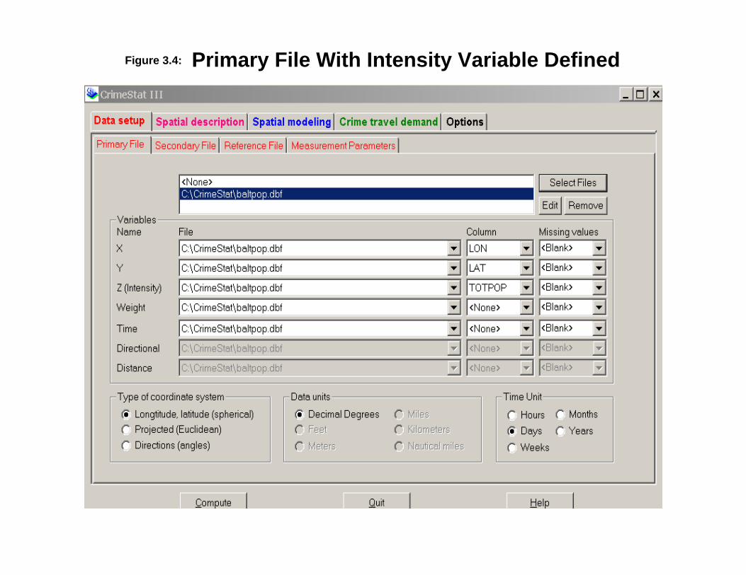
Primary File With Intensity Variable DefinedFigure 3.4:

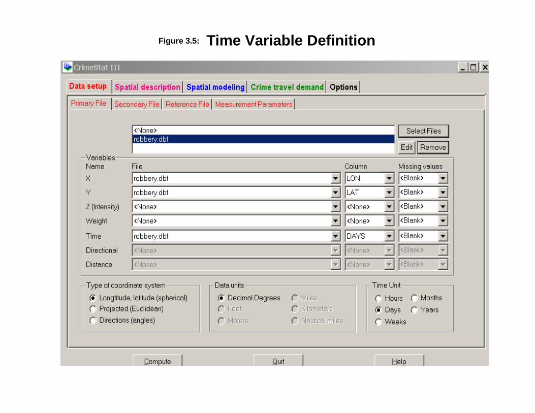
Time Variable DefinitionFigure 3.5:

3.15

P r oje c te d co ord in a te s

Projected coordin a tes a re a rbit ra ry coor din a tes based on a par t icu la r project ion ofthe ea r th to a fla t pla ne. They h ave an arbit ra ry or igin (the pla ce where X=0 and Y=0) andare a lmost a lways defined in u n its of feet or meters.9

Crim eS tat can work with either spher ica l or project ed coordina tes . On the p rimaryfile t ab, th e user indica tes wh ich coordina te syst em is being used. If the coordina te syst emis sph er ical, t hen un it s a re au toma t ically a ssumed to be lat itude and longitude in decima ldegrees. If the coordina te syst em is pr ojected, th en it is n ecessa ry to specify whet her themeasu rem ent u nits a re feet or m eters.

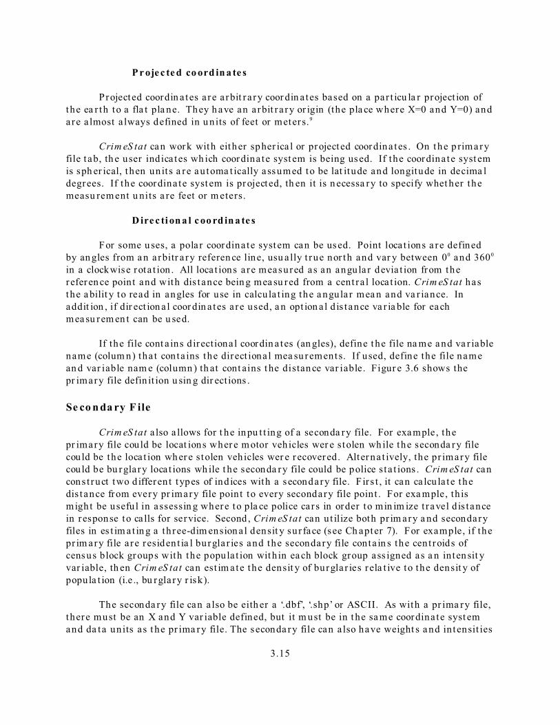
D ire c ti on a l c oo rd in a te s

For some uses, a pola r coordina te syst em can be used. Point loca t ions a re definedby an gles from a n arbitr a ry referen ce line, usu a lly t rue nor th and var y between 00 and 3600

in a clockwise rota t ion . All loca t ions a re measured as an angu la r devia t ion from therefer en ce point and with dis t ance bein g mea su red from a cent ra l loca t ion. Crim eS tat hasthe a bilit y to read in angles for use in calcu la t ing the a ngula r mea n and va r iance. Inaddit ion , if dir ect ion a l coor din a tes a re used, a n opt ion a l d is t ance va r ia ble for eachmea su rem en t can be u sed.

If the file cont a ins d irectiona l coordin a tes (an gles), define t he file na me and va r iablename (colum n) tha t con ta ins the direct iona l mea su rements. If used, define the file namean d var iable nam e (column ) th at cont ains t he distan ce var iable. Figur e 3.6 shows thepr imary file defin it ion u sin g dir ect ions .

Se co n da ry F ile

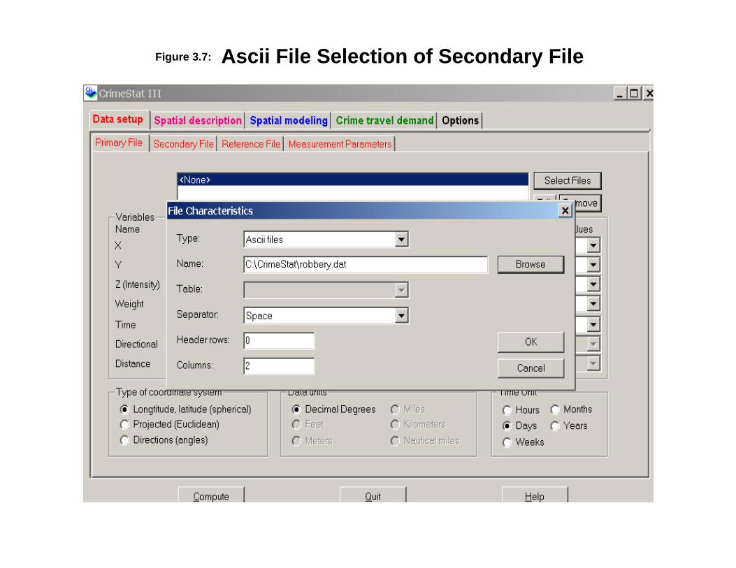
Crim eS tat a lso a llows for t he in pu t t ing of a seconda ry file. For exa mple, thepr imary file could be locat ions wher e m otor veh icles wer e stolen wh ile the seconda ry filecould be the loca t ion wh er e stolen veh icles wer e r ecovered. Alter na t ively, the pr imary filecould be bu rgla ry loca t ions wh ile t he seconda ry file could be police s t a t ions . Crim eS tat cancons t ruct two d ifferen t types of ind ices with a secondary file. F ir s t , it can ca lcu la te thedis tance from every pr imary file point to every secondary file point . For exa mple, th ismight be usefu l in assessin g where to pla ce police car s in order to min im ize t r avel d is t ancein response to ca lls for service. Second , Crim eS tat can u t ilize both pr im ary a nd secondaryfiles in es t im at in g a th ree-dim ension a l densit y sur face (see Ch apter 7). For example, if thepr im ary file a re residen t ia l burgla r ies and the secondary file conta in s the cen t roids ofcensus block groups with the popula t ion wit h in each block group ass igned as a n in ten sit yvar iable, th en Crim eS tat can est im ate the densit y of burgla r ies rela t ive to the densit y ofpopula t ion (i.e ., bu rgla ry r isk).

The seconda ry file can a lso be eith er a ‘.dbf’, ‘.shp’ or ASCII. As with a pr ima ry file,there must be an X and Y var iable defined, but it m ust be in t he sa me coordina te syst emand da ta un its as t he pr ima ry file. The seconda ry file can a lso have weight s a nd in tensit ies

File Definition With Angles (Directions)Figure 3.6:

3.17

assigned, bu t not a t im e va r ia ble.. Figure 3.7 shows the in put t in g of a n ASCII file for theseconda ry dat a set while figure 3.8 shows a cor rect defin ition of the seconda ry file.

Re fere n ce Fi le

Severa l of th e r out ines in Crim eS tat gener a lize the poin t da ta to all loca t ions in thest udy ar ea , in pa r t icu lar the one-var iable and t wo-var iable den sity in terpola t ion rou t ines(chapter 8), and the r isk-adjust ed nea res t neighbor h iera rch ica l clust er ing rou t ine (chapter6). The gen er a liza t ion u ses a refer en ce file placed over the s tudy a rea . The STAC pr ogra malso uses a referen ce file for sea rchin g (cha pt er 7). Typica lly, th e r eferen ce file is arectangula r gr id file (t rue gr id), tha t is a rectangle wit h cells defined by columns a nd r ows.;each grid cell is a rectangle and colum n-row combina t ions a re used. It is possible to use anon-rectangu la r gr id file under specia l circumstances (e.g., a gr id wit h water , m ounta in s orother ju r isdict ions r emoved), but a rectangula r grid would be used in most cases.Crim eS tat can crea te a gr id file direct ly or can rea d in an ext er na l gr id file. F igure 3.9sh ows a grid pla ced over both the County of Balt imore a nd t he City of Balt imore.

Crea ting a Refere nc e Grid

Crim eS tat can also creat e a tr ue grid. There are t wo steps:

1. The user selects Create Grid from the Reference F ile t ab and inpu ts the Xand Y coordin a tes of the lower -left a nd u pper -righ t coord ina tes of the gr id. Th ese coord ina tes must be t he same a s for the pr imary file.

Thus, if the pr imary file is u sin g spher ical (lat /lon) coordin a tes, then the gr id filecoordina tes m ust a lso be lat /lon . Conversely, if the pr ima ry file coordina tes a re pr ojected,then the gr id file coordin a tes must a lso be projected, usin g the same m ea su rem en t un it s(feet or meter s). The lower -left and upper -r igh t coordin a tes a re those from a gr id whichcover s t he geograph ica l a r ea . A user shou ld iden t ify these with a GIS p rogram or from aproperly indexed map. In MapIn fo, t h is is easily done by eit her drawin g a rectangle a roundthe s tudy a rea and double clicking to get informat ion a bout the a rea or by checkin g thecursor pos it ion . In ArcView , you can draw a shape file of the appropr ia te referencerectangle and t hen use t he Coordina te Ut ility scr ipt to get t he X and Y coordina tes.

2. Th e u ser selects whet her the gr id is to be crea ted by cell spacing or by t henumber of columns.

With By cell spacing, the size of the cell is defined by it s h orizonta l widt h , in thesa me unit s a s t he m ea su rem en t un it s of the pr imary file. This would be u sed t o ma inta ina cert a in size of spacing for a cell. For exa mple, if the coordina te syst em is sph er ical a ndthe lower -left coordina tes a re -76.90 and 39.20 degrees a nd t he upper -r igh t coordina tes a re-76.32 and 39.73 degr ees (a gr id which over la ps Ba lt im ore City a nd Ba lt im ore Cou nty),then the hor izonta l distance - the difference in t he two longitudes (0.58 degrees ) must bedivided in to appr opr ia te sized in ter vals. At t h is la t itude, the differ en ce in longitudes is34.02 miles. If a user wanted cell spa cing of 0.01 degrees, th en th is would be ent ered a nd

Ascii File Selection of Secondary FileFigure 3.7:

Secondary File DefinitionFigure 3.8:

Miles

420

Figure 3.9: Grid Cell Structure for Baltimore Region108 Width x 100 Height Grid Cells

Baltimore County

City of Baltimore

D

!

!

Upper-right Coordinate

Lower-left Coordinate

3.21

Crim eS tat would ca lcu la te 59 colu mns (cells) in the hor izonta l d ir ect ion , on e for eachint erval of 0.01 and one for the fract iona l rem ainder . If the coordina te syst em is pr ojected,then sim ila r calcu la t ions would be m ade usin g the projected un it s (feet or m et er s).

Probably an easier way to specify th e grid is to ind ica te the number of colum ns. Bycheckin g By num ber of colum ns, the u ser defines t he n umber of columns t o be calcu la ted. Crim eS tat will au tomat ica lly ca lcu lat e the cell spa cing needed a nd will ca lcu lat e therequired number of rows. For example, usin g th e sa me coordina tes a s a bove, if a userwa nted ha lf mile squares for the cells, then they would n eed approximately 68 cells in thehorizon ta l dir ect ion s ince 34.02 miles divided by 0.5 m ile squ ares equ a ls a bout 68 cells . F igure 3.10 shows a cor rect ly defined r eference file where Crim eS tat crea tes the referencegrid with the number of colum ns being defined; in the exam ple, 100 colum ns a re request ed.

Sa vi n g a Re fere n ce Fi le

The user can save the lower -left and upper -r igh t coordin a tes of a defin ed referencegrid a nd t he number of colum ns. Type Save <filename>. The coordina tes a nd colum n sizeswill be saved in t he syst em regist ry. To load a n a lrea dy defined reference file, type Loadand then check the appropr ia te filename, followed by click in g on ‘Load’.

In addit ion , t he user can save the reference parameter s to an ext erna l file. To doth is, it has t o be alr eady saved in t he syst em regist ry. Type Load and then check theappropr ia te filename, followed by clicking on ‘Sa ve to File”. Define the directory a nd filename a nd click ‘Sa ve’. The file will be sa ved wit h an ‘ref’ ext en sion (e.g.,Ba lt im oreCou nty.ref).

Us e an Ex te rn al Grid Fi le

Many GIS progr ams can crea te un iform gr ids which cover a geogr aphica l a rea . Aswit h the pr im ary a nd secondary files, t hese need to be conver ted to eit her ‘.dbf’, ASCII or ‘.shp’ files. To use an exist in g gr id file crea ted in a GIS or another progr am, t he user clickson From File on t he Referen ce File t ab a nd select s t he file.

There are th ree character ist ics wh ich sh ould be ident ified for an exist ing grid file:

1. The name of the file. The user select s the file from a dia log box s im ila r to thepr ima ry file.

2. If the exist ing reference file is a t rue grid, the T rue Grid box should bechecked.

3. If it is a t rue gr id, t he n umber of columns should be en ter ed. Crim eS tat willau tomat ica lly count the number of records in the file and pla ce it in the Cellsbox. When the n umber of columns is en ter ed, Crim eS tat will au toma t icallycalcu la te t he n umber of rows.

Create Reference Grid SetupFigure 3.10:

3.23

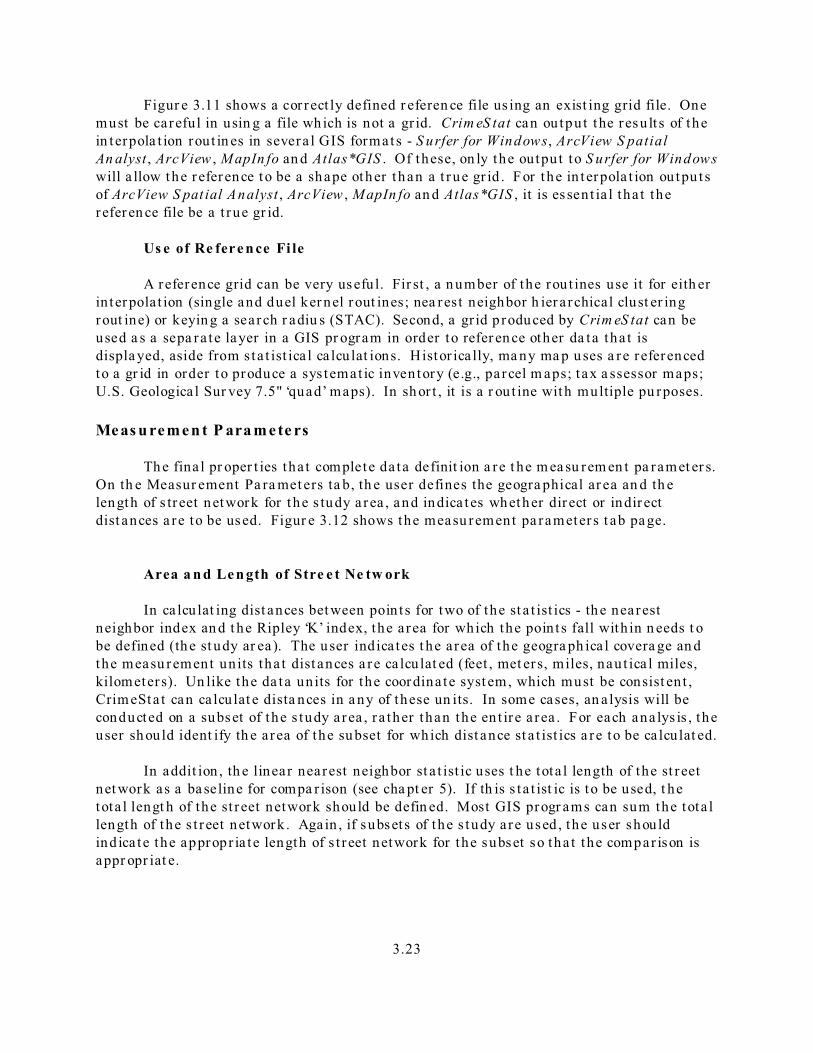
Figur e 3.11 shows a cor rect ly defined r eferen ce file us ing an exist ing grid file. Onemust be careful in usin g a file wh ich is not a gr id. Crim eS tat can ou tpu t the resu lt s of thein terpola t ion rout in es in severa l GIS formats - S urfer for Windows, ArcView S patialAn alyst , ArcView , MapIn fo an d Atlas*GIS . Of these, on ly the outpu t to S urfer for Windowswill a llow the r eference to be a shape other t han a t rue gr id . For t he in t erpola t ion ou tpu t sof ArcView S pat ial Analyst , ArcView , MapIn fo an d Atlas*GIS , it is es sen t ia l tha t therefer en ce file be a t rue gr id.

Us e of Re fere n ce Fi le

A reference grid can be very usefu l. Fir st , a n umber of the rou t ines use it for eith erin ter pola t ion (single and duel ker nel rout ines; nea rest neighbor h ier a rchical clust er ingrout ine) or keyin g a sea rch r adiu s (STAC). Second, a gr id p roduced by Crim eS tat can beused a s a sepa ra te layer in a GIS pr ogram in order to refer en ce other da ta tha t isdispla yed, aside from s ta t ist ica l ca lcu lat ions. Histor ica lly, ma ny ma p u ses a re referencedto a gr id in order to produce a sys temat ic inventory (e.g., pa rcel m aps; t ax a ssessor maps;U.S. Geologica l Sur vey 7.5" ‘quad’ maps). In sh or t , it is a r ou t ine with multiple pu rposes.

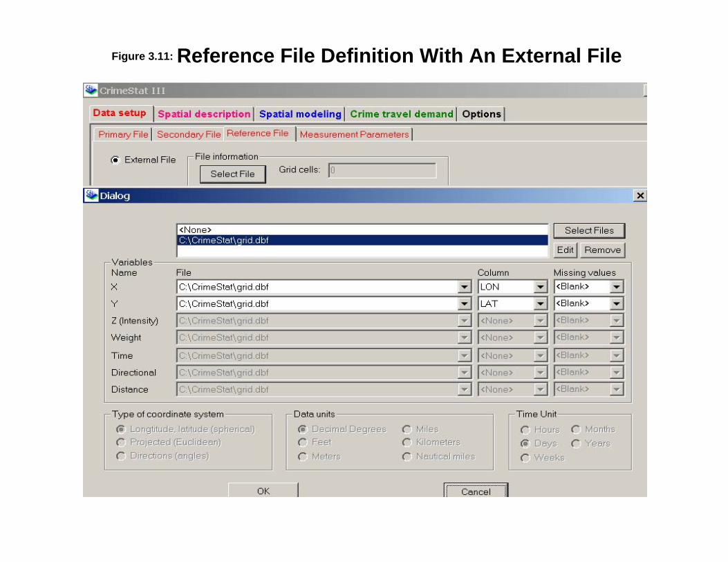
Me as u rem e n t P ara m e te rs

Th e fina l pr oper t ies tha t complete da ta definit ion a re t he m ea su rem en t pa ramet er s. On th e Measur ement Pa ra met ers ta b, th e user defines the geogra phical ar ea an d th elength of s tr eet network for t he s tudy a rea , and indica t es whether dir ect or indir ectdist ances a re to be used. Figur e 3.12 shows the measu rement pa rameters t ab pa ge.

Area a n d Le n gth of Stre e t Ne tw ork

In ca lcu lat ing dist ances bet ween poin t s for two of the st a t ist ics - th e nearestneighbor index an d t he Ripley ‘K’ index, the area for which the poin t s fall with in n eeds t obe defined (th e st udy ar ea). The user indica tes t he area of the geogra ph ica l covera ge an dthe measu rement un its tha t dist ances a re ca lcu lat ed (feet , met ers, miles, nau t ica l miles,kilometers). Un like the da ta un its for the coordina te syst em, which must be consist en t ,Crim eSta t can ca lcu lat e dista nces in a ny of these un its. In some cases, an a lysis will beconducted on a subset of the s tudy a rea , r a ther than the en t ire a rea . For each ana lys is , theuser sh ould ident ify th e area of the su bset for which dist ance st a t ist ics a re to be ca lcu lat ed.

In addit ion , th e linear nearest neighbor st a t ist ic uses t he tota l length of the st reetnet work as a ba seline for compa r ison (see cha pt er 5). If th is s t a t ist ic is to be used, t hetota l lengt h of the st reet network should be defin ed. Most GIS progr ams can sum the tota llength of the s t reet network . Aga in , if subset s of the s tudy a re used , the user shou ldind ica te the appropr ia te length of s t reet network for the subset so tha t the compar ison isappr opr iat e.

Reference File Definition With An External FileFigure 3.11:

Measurement Parameters PageFigure 3.12:

3.26

Ty pe o f D is ta n ce Me a su re m e n t

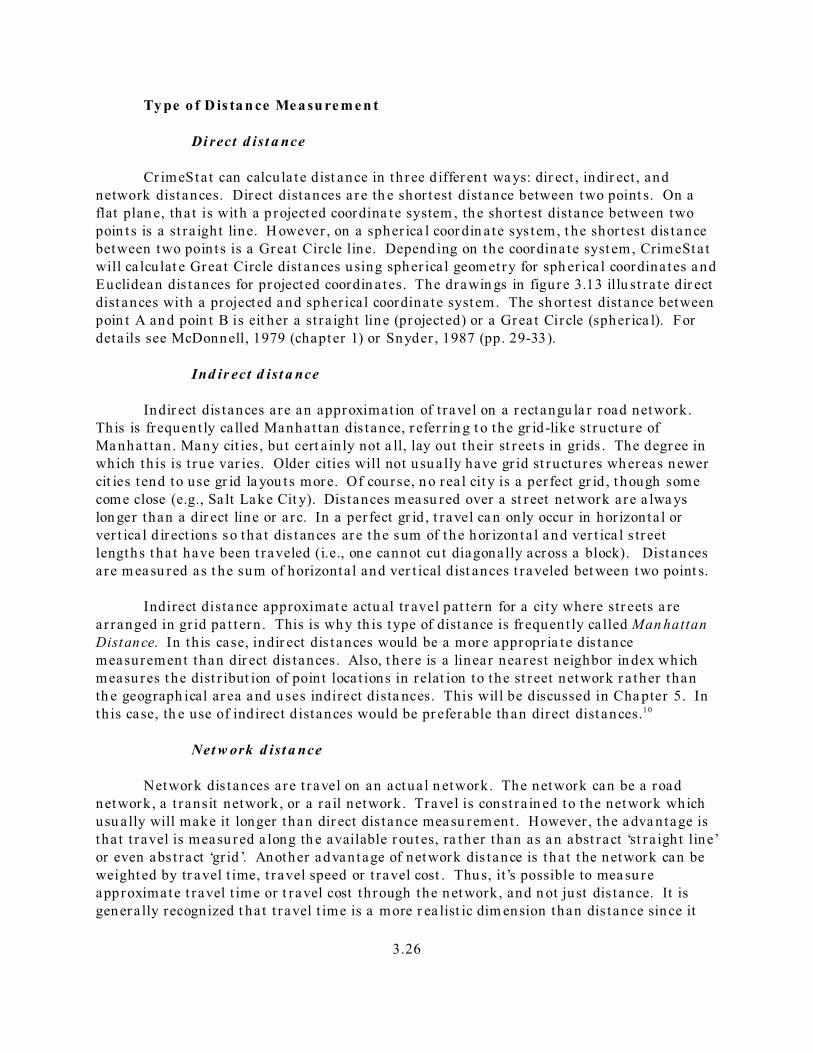
Di rect d ist a nce

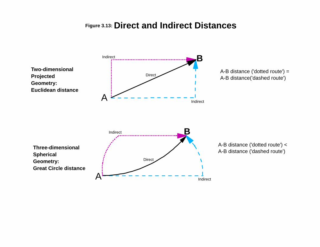
Cr imeSta t can calcu la te dist ance in th ree d iffer en t wa ys: dir ect , indir ect , andnetwork distances. Direct distances a re th e shor test distance between two point s. On aflat plan e, tha t is with a p rojected coordina te system , th e shor test distance between twopoin t s is a st ra igh t line. H owever , on a spher ica l coor din a te sys tem, t he shor test dis t ancebetween two poin t s is a Grea t Circle line. Depend ing on the coordina te syst em, CrimeSt a twill ca lcu lat e Grea t Circle dist ances u sing spher ica l geomet ry for sph er ica l coordina tes a ndEuclidean dis t ances for projected coordin a tes. The drawin gs in figure 3.13 illu st ra te dir ectdist ances with a pr ojected a nd spher ica l coordina te syst em. The sh or test dist ance betweenpoin t A and poin t B is eit her a st ra igh t line (projected) or a Grea t Circle (spher ica l). Fordeta ils see McDonnell, 1979 (chapter 1) or Snyder , 1987 (pp. 29-33).

Ind ir ect d ist a nce

Indir ect dis tances a re an approximat ion of t r avel on a rectangu la r road network.This is frequent ly ca lled Manha t tan dis t ance, r efer r in g t o the gr id -like st ructure ofMa nha t tan . Many cit ies, bu t cert a in ly not a ll, lay out their st r eet s in grids . The degree inwhich th is is t rue var ies. Older cities will not u su a lly have gr id st ructures wh ereas n ewercit ies t end to use gr id la you ts more. Of course, n o rea l city is a per fect gr id , t hough somecome close (e.g., Sa lt La ke Cit y). Dis tances m ea su red over a st reet net work are a lwa yslon ger than a dir ect line or a rc. In a per fect gr id , t r avel ca n only occur in hor izonta l orver t ica l d ir ect ions so tha t dis t ances are the sum of t he hor izon ta l and ver t ica l s tr eetlengths t ha t have been t raveled (i.e., one cannot cu t diagona lly across a block). Distancesare m ea su red as t he sum of horizonta l and ver t ical dist ances t r aveled bet ween two point s.

Indirect dista nce approximat e actu al tr avel pat tern for a city where str eets a rea r ranged in gr id pa t t ern . This is why th is type of dist ance is frequent ly ca lled Man hattanDistance. In th is case, indir ect dis t ances would be a more appropr ia te dis t ancemeasurement than dir ect dis t ances. Also, t here is a linear nearest neighbor in dex whichmeasu res t he dist r ibut ion of poin t loca t ions in relat ion to the st reet network r a ther thanth e geograph ical ar ea a nd u ses indirect dista nces. This will be discussed in Cha pter 5. Inth is case, th e use of indirect d ist ances would be pr eferable th an direct dist ances.10

Net w ork d ist a nce

Network dis t ances a re t r avel on an actua l n etwork. The network can be a roadnetwork, a t r ansit network, or a ra il network. Travel is const ra in ed to the network whichusu a lly will make it longer than dir ect dis t ance mea su rem en t . However , the adva ntage istha t t r avel is measu red a long th e available r ou tes, ra ther than as a n abst ract ‘st ra igh t line’or even abs t ract ‘gr id ’. Another advan tage of network dis tance is tha t the network can beweight ed by tr avel t ime, t r avel speed or t r avel cost . Thu s, it’s possible to mea su reapproximate t r avel t ime or t r avel cost th rough the net work, and n ot just dis t ance. It isgener a lly recognized t ha t t r avel t ime is a more r ea list ic dim en sion than dis t ance since it

A

B

A

B

Two-dimensionalProjectedGeometry:Euclidean distance

Three-dimensionalSphericalGeometry:Great Circle distance

A-B distance ('dotted route') =A-B distance('dashed route')

A-B distance ('dotted route') <A-B distance ('dashed route')

Direct

Direct

Indirect

Indirect

Indirect

Indirect

Direct and Indirect DistancesFigure 3.13:

3.28

will va ry by t im e of day. For exa mple, it genera lly t akes a lot lon ger to t r avel a ny dis t ancein an u rban a rea dur ing the peak even ing ‘rush hours ’ (4-7 PM) than a t , say, 3 AM in themorn ing. Dist ance is a lwa ys in var ian t wh er ea s t r avel t ime va r ies. An even more r ea list icdim ension t ravel is cost . Tr ips over a met ropolit an a rea a re governed by a number ofvar iables aside from t ravel t ime - vehicle oper a t ing cost s, pa rking cost s a nd, even , likelyr isk cost s (e.g., likelihood of being caught ). For an offender who is t r aveling, th ose oth ercos t factor s may be a s impor t an t a s t he actua l t ime it t akes in det ermin ing whether t omake a cr im e t r ip . In chapter 15, t here is a discussion of t r avel cos t s in the context oftr avel decisions.

Ther e a re t wo major disadva ntages in usin g network dis t ance, however . Fir st ,there are er ror s in networks . For exam ple, a n etwork m ay not h ave incorpora ted a ll newroads or conver ted roads. Thus, t he network a lgor it hm will n ot choose a par t icu la r routewhen, in fact , it actua lly exist s a nd people use it . It’s crit ica l th a t networks be upda ted t oensu re accuracy. See chapt er 12 for a discuss ion of network er rors a nd t he need t othorough ly clean them.

Second, it can take a long time to ca lcu lat e dist ance a long a n etwork. The sh or testpa th a lgor ithm tha t is u sed m ust explore m any alter na t ive rout ines, a t ime consu mingprocess. F or sim ple st a t is t ics , t h is is not liable to be a problem. But , for some of the morecomplica ted mat r ix opera t ion s (e.g., t he dis t ance fr om every poin t to every ot her poin t ),ca lcu la t ion t ime increases exponen t ia lly with the number of ca ses . I’ve had runs tha t t ookfive da ys on a fas t compu ter . For a ny complex calcu la t ion, it becomes impr actica l to ha veto wait a long t ime just for a lit t le ext ra pr ecision . In sh ort , it may not be wor th the t rouble. At some point in th e near futu re, we will ha ve 64 bit operat ing systems a nd su per-fastcomputer s . At t ha t poin t , runn ing a ll ca lcu la t ions on a network may be a much morepr act ica l proposition . For now, I highly recommend t ha t network d istance be usedspar ingly for calculat ions.

D is ta n ce Ca lc u la tio n s

Distances in Cr imeSta t a re calcula ted wit h the followin g form ulas:

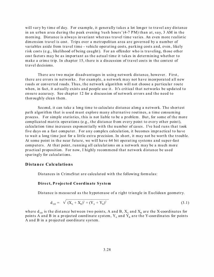
D ire c t, P r oje c te d Co ord in a te S ys te m

Distance is m ea su red as t he h ypoten use of a r igh t t r iangle in Euclidea n geomet ry. ______________________

dAB = % (XA + XB)2 + (YA + YB)2 (3.1)

where dAB is t he dist ance bet ween two point s, A and B, XA an d XB ar e the X-coordina tes forpoin t s A and B in a pr ojected coord ina te syst em , YA an d YB a r e t he Y-coordina tes for poin t sA and B in a project ed coordina te sys t em.

3.29

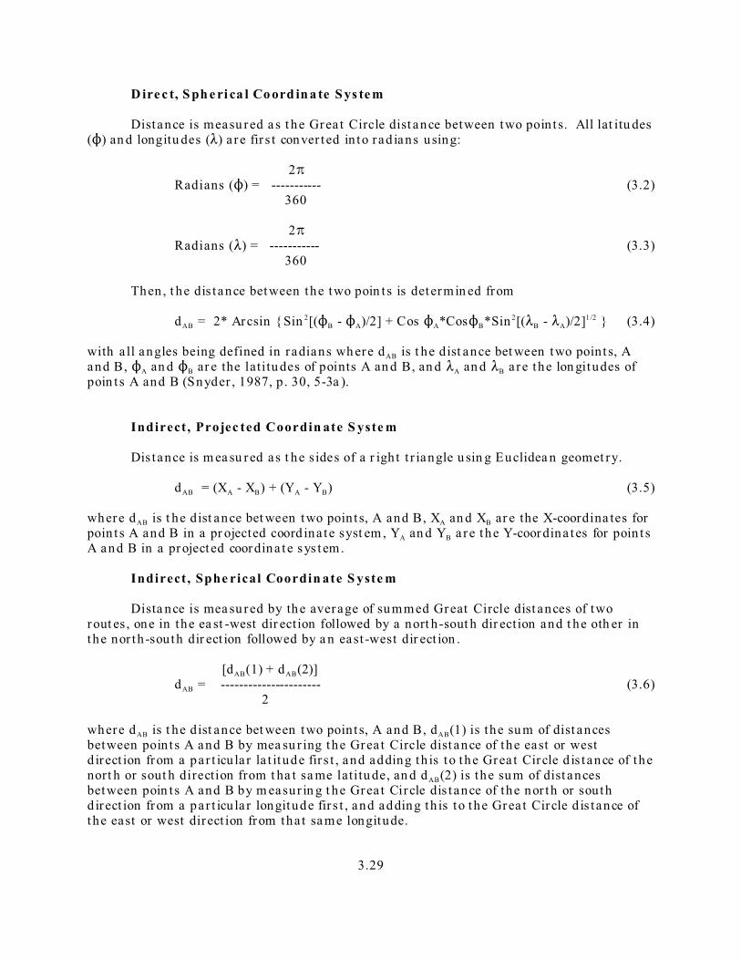
D ire c t, S ph e ri ca l Co ord in a te S ys te m

Distance is measu red a s t he Grea t Circle dist ance between two poin t s. All lat itu des(N) an d longitu des (8) a re fir s t conver ted in to rad ians using:

2BRadians (N) = ----------- (3.2)

360

2BRadians (8) = ----------- (3.3)

360

Then , t he dis t ance between the two poin t s is determin ed from

dAB = 2* Arcsin { Sin 2[(NB - NA)/2] + Cos NA*CosNB*Sin 2[(8B - 8A)/2]1 /2 } (3.4)

with a ll angles being defined in radians wh ere dAB is t he dist ance bet ween two point s, Aand B, NA an d NB ar e the latitu des of points A an d B, an d 8A an d 8B a re the lon gitudes ofpoin t s A and B (Snyder , 1987, p . 30, 5-3a ).

Indirect , Projec ted Coordin ate S yste m

Distance is m ea su red as t he s ides of a r igh t t r iangle u sin g Euclidea n geomet ry.

dAB = (XA - XB) + (YA - YB) (3.5)

where dAB is t he dist ance bet ween two point s, A and B, XA an d XB ar e the X-coordina tes forpoin t s A and B in a pr ojected coord ina te syst em , YA an d YB a r e t he Y-coordina tes for poin t sA and B in a project ed coordina te sys t em.

Indirect , Sphe rical Coordin ate S yste m

Dista nce is mea su red by the average of summed Great Circle dist ances of tworout es, one in the ea st -west dir ection followed by a nort h-sout h dir ection and t he oth er inthe nor th-south dir ect ion followed by a n east -west dir ect ion .

[dAB(1) + dAB(2)]dAB = ---------------------- (3.6)

2

where dAB is t he dist ance bet ween two point s, A and B, dAB(1) is the su m of dist ancesbetween poin t s A and B by mea su r ing the Grea t Circle dist ance of the east or westd irect ion from a par t icu la r la t itude fir s t , and adding th is to the Grea t Circle d is tance of thenort h or sout h direction from t ha t sa me latitu de, an d dAB(2) is the su m of dist ancesbetween poin t s A and B by m easur in g t he Grea t Circle dis t ance of the nor th or southd irect ion from a par t icu la r longitude fir s t , and adding th is to the Grea t Circle d is tance ofthe east or west direct ion from tha t sa me longitude.

3.30

Netw ork Dis tance

Net work d istance is ca lcu lat ed with a sh or test pa th a lgor ith m. Cha pt ers 12 and 16provide more in format ion on networks and how dis tance is ca lcu la ted on them. A shor tsu mmary will be given here. In genera l, dist ance is ca lcu lat ed by a shor test pa tha lgor ithm. In a shortest path for a sin gle t r ip (from a sin gle or igin to a sin gle dest in a t ion ),the r out e wit h the lowest over a ll im pedance is selected. Impeda nce can be defined in t ermsof dis t ance, t r avel t im e, speed, or genera lized cost .

There are a number of sh or test pa th a lgor ith ms t ha t have been developed(Sedgewick, 2002). They differ in ter ms of wh et her they a re br ea dt h-fir st (i.e., sea rch a llpossibilities) or dept h-firs t (i.e., go st ra igh t to the ta rget) algor ith ms a nd wh ether theyexa min e a one-to-many r ela t ion sh ip (i.e., from a sin gle or igin node to many n odes) or amany-t o-many r ela t ion sh ip (All pa ir s; from ea ch node to every ot her node).

The a lgor ith m tha t is most commonly used for sh or test pa th ana lysis of moder a te-sized da ta set s (up t o a million cases) is ca lled A*, which is pronounced “A-sta r” (Nilsson ,1980; Stout , 2000; Rabin 2000a , 2000b; Sedgewick, 2002). It is a one-to-many algor ithmbut is an improvemen t over a nother commonly-used a lgor ith m ca lled Dijkstra (Dijkst ra ,1959). Ther efore, I’ll st a r t firs t by describing the Dijk st ra a lgorit hm before expla in ing theA* a lgor ithm.

D i jk s t r a a l g or i t h m

The Dijkst r a a lgor ithm is a one-to-many sea rch st r a t egy in wh ich a shor t es t pathfrom a s ingle node to a ll other nodes is ca lcu la ted . The rou t ine is a bread th-fir s t a lgor ithmin tha t it sea rches a ll possible pa ths, bu t it bu ilds the pa th one segmen t a t a t ime. St a r t ingfrom an or igin loca t ion (node), it iden t ifies the node tha t is nea res t t o it a n d which has nota lr eady been iden t ified on the shor test pa th . Aft er each node has been iden t ified to be onthe short est pa th , it is r em oved from the sea rch possibilit ies. The a lgor ithm pr oceeds u n t ilthe short es t pa th to all n odes has been deter mined.

The a lgor ithm can a lso be st ructu red to find t he short est pa th bet ween a pa r t icula ror igin node and a par t icu la r dest in a t ion node. In th is case, it will qu it once the dest in a t ionnode h as been ident ified on the sh or test pa th . The a lgor ith m can a lso be st ructured t ofind the shor t es t path from each or igin node to each des t ina t ion node. It does th is one patha t a t ime (e.g., it finds the short est pa th from node A to all other nodes; th en it finds theshor test pa th from node B t o a ll other nodes; and so forth ).

A* Al gor i t h m

The biggest problem with t he Dijkst ra algorith m is th at it sear ches th e path toever y sin gle node. If the purpose wer e t o find t he short est pa th from a sin gle node to allother nodes, t hen th is would produce the best solu t ion . H owever , wit h a mat r ix of dis t ancefrom one set of poin t s to another set of poin t s (an or igin -des t ina t ion mat r ix), we rea llywa nt to kn ow the dist ance bet ween a pa ir of nodes (one origin and one dest ina t ion). Consequ en t ly, the Dik jst ra a lgorit hm is very, very slow compa red to what we n eed . Itwould be a lot qu icker if we could find the dist ance from each or igin-dest ina t ion pa ir one a ta t ime, but quit t he algorith m a s soon a s th at dista nce has been determined.

3.31

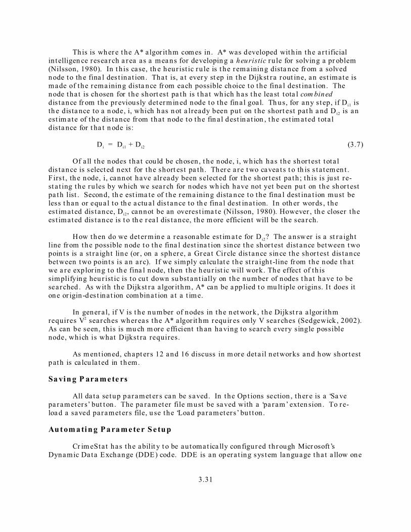
Th is is wh er e t he A* a lgor ithm comes in . A* was developed wit h in the a r t ificialin telligen ce resea rch a rea as a mea ns for developin g a heuristic ru le for solving a pr oblem(Nilsson, 1980). In t h is case, th e heur ist ic ru le is t he remaining dista nce from a solvednode to th e fina l des t ina t ion . Tha t is, a t ever y st ep in the Dijkst ra rout ine, an est imate ismade of the remaining dista nce from each possible choice to the fina l dest ina t ion . Thenode tha t is chosen for the short est pa th is t ha t wh ich h as t he lea st tota l com bineddis tance fr om the previously determin ed node to the fin a l goal. Th us, for any s tep, if D i1 isth e dista nce to a n ode, i, which h as n ot a lready been put on t he short est pat h a nd D i2 is anest im ate of the dis t ance from tha t node to the fin a l dest in a t ion , t he est im ated tota ldista nce for t ha t n ode is:

D i = D i1 + D i2 (3.7)

Of a ll the nodes tha t could be chosen , t he node, i, which has the shor test tota ldis t ance is select ed next for the short es t pa th . Ther e a re t wo cavea t s t o th is s t a tem en t . F irs t , th e node, i, cannot have alr eady been selected for the sh or test pa th ; th is is just re-st a t ing the ru les by which we sea rch for nodes wh ich have not yet been pu t on the sh or testpa th list . Second, th e est ima te of the remaining dista nce to the fina l dest ina t ion must beless t han or equ a l to th e a ctu a l dis t ance to th e fina l dest ina t ion. In oth er words , theest imated dis t ance, Di2, cannot be an overes t ima te (Nilsson, 1980). However , th e closer theest imated dis t ance is t o th e r ea l dis t ance, the m ore efficient will be the sea rch.

How then do we determin e a reasonable est im ate for D i2? The a nswer is a st ra ightline from the possible node t o the fina l dest ina t ion since the sh or test dist ance between twopoin t s is a st ra igh t line (or , on a sphere, a Grea t Circle dis t ance sin ce the shor test dis t ancebetween two poin t s is a n a rc). If we simply ca lcu lat e the st ra igh t -line from the node t ha twe a re explor ing to th e fina l node, then the heu r ist ic will work. The effect of th issimplifying heu r ist ic is to cu t down su bst an t ially on the number of nodes t ha t have to besearched . As with the Dijkst ra a lgor ithm, A* can be a pp lied t o mu lt iple or igins. I t does itone or igin -des t ina t ion combina t ion a t a t ime.

In gener a l, if V is t he number of nodes in the net work, the Dijkst ra a lgor ithmrequires V2 sea rches whereas the A* algor it hm requir es only V searches (Sedgewick , 2002).As can be seen, this is mu ch m ore efficient th an ha ving to search every single possiblenode, which is what Dijkst ra requires.

As m ent ioned, chapt ers 12 and 16 discuss in m ore det a il networks and h ow sh or testpath is ca lcu la t ed in them.

Sa vin g P ara m e te rs

All da ta setup paramet er s can be saved. In the Op t ions section , ther e is a ‘Sa vepa rameters’ but ton . The pa rameter file must be saved with a ‘pa ram’ exten sion . To re-loa d a saved parameter s file, u se the ‘Load parameter s’ bu t ton .

Au t om a ti n g P a ra m e te r S e tu p

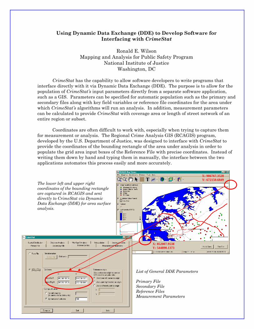
Cr im eSta t has the abilit y t o be au tomat ica lly configured th rough Micr osoft ’sDynamic Data Exchange (DDE) code. DDE is an opera t ing sys tem language tha t a llow one

3.32

applica t ion to call up another . The DDE code in Cr im eSta t a llows the defin in g of thepr ima ry var iable, th e seconda ry var iable, th e reference file, and t he measu rementparameter s. Appendix A gives the specific code in st ruct ion s. Ron Wilson’s exa mple belowillu st ra tes how Cr im eSta t can be linked to another applica t ion .

S ta tis tic al R ou t in e s an d Ou t pu t

St a t ist ical r out ines a re selected from the t wo groupin gs of st a t ist ics - Spa t ia lDescription a nd Spa tial Modeling. The user selects t he routines and inpu ts a nypa rameters, if required . Clickin g on the Compu te but ton a ll the rou t ines tha t have beenselected. Since CrimeSt a t is multi-th readed, differen t rou t ines run in separa te th readsand m ay finish a t differen t t imes . When a rou t ine is fin ished, a F inish ed m essa ge will bedispla yed a t the bot tom of th e screen .

Virtu ally all th e rout ines out put to eith er GIS packa ges or t o sta nda rd ‘dbf’ fileswhich can be read by spreadsheet , da ta base, a nd gr aphics progr ams. While each outpu tt able can be pr in ted as an Ascii file to a pr in ter , it is recommended tha t the user outpu t theresu lts in ‘dbf’ and r ead it int o a pr ogra m tha t has bet t er ou tpu t capa bilit ies. For exam ple,the nearest neighbor and Ripley’s K rout in es outpu t columns can be saved as st andard ‘dbf’files which can be rea d by spr eadsh eet pr ogra ms, such as E xcel or Lotus 1-2-3. Thespreadsheet da ta , in tu rn , ca n be im por ted in to most gr aphics progr ams, such asPowerPoint or Freelan ce, for crea t ing bet t er qua lity gra ph ics. For ‘cu t -and-pas te’opera t ions , user can copy por t ions of the ou tpu t t ables and paste them in to word processingpr ogra ms. One should see Cr imeSta t as a collect ion of specialized st a t ist ica l rout ines tha tcan p roduce ou tpu t for other p rograms , ra ther than as a fu ll-blown package.

A Tutoria l w i th the Sample Data Set

Let ’s run th rough the da ta setup and runnin g of severa l r out in es wit h one of thesa mple dat a set s t ha t were pr ovided (Sam pleDat a .zip). Unzipping th is file reveals t wofiles called Inciden t.dbf an d BaltPop.dbf. The incident file is a collect ion of inciden tloca t ions tha t have been randomly s imula ted with the other file includes the 1990popula t ion of cen su s block groups in the Ba lt imore region.

1. St a r t the Crim eS tat pr ogra m by either double-clickin g on the Crim eS tat iconon t he desktop (if inst a lled) or else open ing Windows Explorer and loca t ingthe directory wher e Crim eS tat is st ored a nd double-clickin g on the file ca lledcrim estat.exe.

2. Once the pr ogra m spla sh pa ge closes, t he user will be lookin g at the DataS e tu p pa ge with the Pr ima ry File page open .

3. Click on ‘Select F iles’ followed by ‘Browse’. Loca te the file ca lled Incident .dbfand click on ‘Open’ followed by ‘OK’.

4. The file na me will n ow be list ed for the X, Y, Z(int en sit y), Weight , and Tim efields. Th is va r iable, however , on ly has t h ree fields - ID, Lon, La t , indicat ingan record number , t he lon gitude and la t it ude of the in ciden t loca t ion .

Using Dynamic Data Exchange (DDE) to Develop Software for Interfacing with CrimeStat

Ronald E. Wilson

Mapping and Analysis for Public Safety Program National Institute of Justice

Washington, DC

CrimeStat has the capability to allow software developers to write programs that interface directly with it via Dynamic Data Exchange (DDE). The purpose is to allow for the population of CrimeStat’s input parameters directly from a separate software application, such as a GIS. Parameters can be specified for automatic population such as the primary and secondary files along with key field variables or reference file coordinates for the area under which CrimeStat’s algorithms will run an analysis. In addition, measurement parameters can be calculated to provide CrimeStat with coverage area or length of street network of an entire region or subset.

Coordinates are often difficult to work with, especially when trying to capture them

for measurement or analysis. The Regional Crime Analysis GIS (RCAGIS) program, developed by the U.S. Department of Justice, was designed to interface with CrimeStat to provide the coordinates of the bounding rectangle of the area under analysis in order to populate the grid area input boxes of the Reference File with precise coordinates. Instead of writing them down by hand and typing them in manually, the interface between the two applications automates this process easily and more accurately. The lower left and upper right coordinates of the bounding rectangle are captured in RCAGIS and sent directly to CrimeStat via Dynamic Data Exchange (DDE) for area surface analysis.

List of General DDE Parameters Primary File Secondary File Reference Files Measurement Parameters

X: 852007.9538 Y: 544890.1373

X: 986767.3528 Y: 672150.6849

3.34

5. Iden t ify the appropr ia te fields under the Column headin g by click in g on thecell and scrolling down to th e a ppropr ia te n ame. For t he X var iable, t hereleva nt name is Lon. For t he Y var iable, t he r eleva nt name is La t (i.e.,tha t ’s t he names u sed in th is file. However, t he var iables will not a lways besim ply n amed). For t h is exa mple, ther e a re no in ten sit y, weigh t or t imevar iables.

6. Un der Type of Coordina te System, be sur e tha t ‘Longitu de/latitude(spherical)’ is checked since this dat a set u se spherical coordina tes.

7. Becau se the coordina te system ar e spherical, th e data un its ar eau tomat ica lly decimal degrees. If th ey were pr ojected, one would have tochoose the pa r t icu la r un it s - feet , meter s , miles , k ilometers , or nau t ica lmiles .

8. Th is fin ish es the set up for the pr imary file. Click on the Seconda ry File t ab.

9. Again , click on select files, loca te a nd open the Ba ltPop.dbf file.

10. On ce loaded, t h is file h as s ix var iables : Blockgr oup , lon, la t , a rea , anddensit y.

11. Define t he pa r t icu lar var iables. For t h is file, the X var iable is Lon and t he Yvar iable is La t . Also, define a Z (in ten sit y) var iable with Totpop. Note , tha tyou cou ld a lso assign th is name to the Weigh t va r iable. Whether thepopula t ion va r ia ble is assigned to the In tensit y or Weight va r ia ble does notmat ter to the ca lcu la t ion . H owever , do not a ss ign th is name to both thein tensit y a nd the weight (i.e., only use one). This fin ishes the setup for theseconda ry var iable.

12. Click on t he Refer en ce File t ab. For t hese da ta , you will define a rectangletha t covers the study a rea by ident ifyin g t he X and Y coordin a tes for thelower -left corner of the rectangle and the upper -r igh t corner of therectangles. The followin g coor din a tes will work:

X YLower -left corner -76.91 39.19

Upper -r igh t corner -76.32 39.72

13. You will a lso need to t ell t he p rogram how many columns you wan t it t ocalcula te. The defau lt value of 100 is fine. If you wa nt it finer , type in ala rger number . If you wa nt it cru der , type in a sm aller number . Thisfinishes th e Reference File setu p.

14. Clock on the Measurement Parameters t ab. There a re th ree pa rameters tha thave t o be defined.

3.35

A. For many rout ines , an a rea est ima te is needed. For t h is sa mple set ,684 square m iles works.

B. For t he linear near est neighbor st at istic only, th e progra m n eeds th etota l len gth of the s t reet net work. In th is da ta , the t ota l st r eet len gthof the Tiger Files for Ba lt imore Cit y and Balt imore county are 4868.9miles .

C. F in a lly, the type of dis t ance measurement has to be defin ed, d ir ect orindirect. For th is exam ple, use d irect m easu rement .

15. The da ta setup is now fin ished. If you want to re-use th is da ta setup, click onthe Opt ions pa ge an d ‘Sa ve par ameters’. Define a file name and be su re togive it a ‘param’ ext ension (e.g., SampleData .param). The next t im e youwant to run th is da ta set , all you’ll need t o do is click on t he Op ti on s pa ge,click on ‘Load parameters ’, and click on the name of the pa rameters file tha tyou sa ved.

16. You a re now ready to run some s ta t is t ics . For th is example, we’ll run on lyfour sta tistics.

17. F irs t , click on t he Spat ia l Descr iption page and then click on the Spa t ia lDis t r ibu t ion t ab.

1. Check the Mean cen ter and standard dis t ance (Mcsd) box. Then , clickon the ‘Save resu lt to’ bu t ton and iden t ify which GIS progr am you arewr it in g t o (ArcView/ArcGis ‘shp’; At la s*GIS ‘BNA’; or MapInfo ‘MIF)and give it a name (e.g., SampleData ).

2. Also, check the Standa rd devia t iona l ellipse (Sde) box and, s imila r ly,choose a file ou tpu t with a name. You can use the same name (e.g.,Sa mpleDa ta ). Crim eS tat will a ssign a un ique prefix to each gr aphica lobject .

18. Second, click on t he ‘Hot Spot’ Ana lysis I t ab. Then , check t he Nea restNeighbor H iera rch ica l Clust er ing (Nn h) box. For t h is exam ple, keep t hedefau lt search r adius, minimu m points per cluster, and n um ber of sta nda rddeviat ions for the ellipses. Also, click on ‘Sa ve ellipses to’, select a GIS fileou tpu t , and give it a name. Aga in , you can use the same name as with theoth er sta tistics.

19. Third , click on t he S pa ti al Mo de li ng pa ge a nd t hen the In ter pola t ion t ab. Check t he duel ker nel densit y inter pola t ion box. Th is r out ine will in ter pola tethe in ciden t dis t r ibu t ion (pr im ary file) rela t ive to the popula t ion dis t r ibu t ion(seconda ry file). For t his exam ple, keep the defau lt kernel para met ers (th eseare expla in ed in more deta il in chapter 8). H owever , be sure to check theUse int ensity var iable box towar ds t he bot tom. This ensu res t ha t the du elkernel r out in e will u se the popula t ion va r ia ble tha t you assigned when youset up t he seconda ry file.

3.36

20. You a re now ready to run the s t a t is t ics . Click on the ‘Compute’ bu t ton . Therout in e will r un un t il a ll four rout in es tha t you selected are fin ished; thet ime will depen d on the speed of your compu ter .

21. Each of the out pu t s a re disp layed on a sepa ra te r esu lt s t ab. You can pr in tany of these resu lt s by click in g on ‘Save to text file’ (one a t a t im e).

22. You can also display the graph ical objects creat ed by th e rout ine in your GIS.Click on ‘Close’ to close the resu lt s window. Then , br ing up your GIS andfin d the object s crea ted by t h is run . There will be a number of gr aphica lobject s a ssocia ted wit h the m ea n center rout ine (having pr efixes of Mc, Xyd,Sdd, Gm, a nd Hm; see chapter 4 for deta ils). There will be two gr aphica lobject s a ssociat ed with the nearest neighbor clus ter ing rou t ine (with pr efixesof Nn h1 and Nnh2). Fina lly, th ere will be a gr id object crea ted by th e du elker nel rout ine wit h a Dk pr efix. You can load t hese object s in and d isp layth em along with th e data file. For t he duel kernel grid, you will need tograph the va r iable ca lled “Z” to see t he pa t t er n .

23. For example, figur e 3.14 shows an ArcView ® map of 1996 veh icle t hefts inBalt imore City and Ba lt imore County a long with the s t andard devia t iona lellipse of the veh icle t hefts, calcula ted wit h Crim eS tat. Crim eS tat ou tpu t sthe ellipse as a shape file, which is then brough t dir ect ly in to ArcView . Asim ila r outpu t could have been done for MapIn fo®. Most of the st a t ist ics inCrim eS tat ha ve similar visua l represent at ions t ha t can be displayed in a GISprogram.

24. When you are finished wit h Crim eS tat, click on ‘Qu it ’ to exit the progra m.

Th is fin ish es the qu ick t u toria l. Crim eS tat is very easy to set u p an d to run . In t henext cha pt er , the focus will be on the st a t ist ics in the program, st a r t ing with the ana lysisof spat ial distr ibut ions.

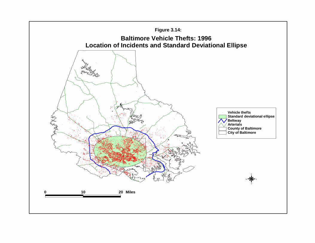
Figure 3.14:

#

#

#

#

#

#

#

#

#

#

#

#

#

#

#

#

#

#

#

#

#

#

#

#

#

#

#

#

#

#

#

#

#

##

#

#

#

#

#

#

#

#

#

#

#

#

#

#

#

#

#

#

#

#

#

#

#

#

#

##

#

#

#

#

#

#

#

#

#

#

#

#

#

#

#

#

#

#

#

#

##

#

#

#

#

# #

#

##

#

#

#

#

#

#

#

#

#

#

#

#

#

#

#

#

#

#

#

#

#

# #

#

#

#

#

#

#

#

#

#

#

#

#

#

#

#

#

#

#

#

#

#

#

#

#

#

#

#

#

#

#

#

#

#

#

#

#

#

#

#

#

#

#

#

#

#

#

#

#

#

#

#

#

##

#

#

#

#

#

#

#

#

#

#

##

#

#

#

#

#

#

#

#

#

#

#

#

#

#

#

#

#

#

#

#

#

#

#

#

#

#

#

#

#

#

#

#

#

#

#

#

#

#

#

#

#

#

#

#

#

#

#

#

#

#

#

#

#

#

#

#

#

#

#

#

#

#

#

#

#

#

#

#

#

##

#

#

#

#

#

#

#

#

#

#

#

#

#

#

#

#

#

#

#

#

##

#

#

#

#

#

#

#

#

#

#

#

#

#

#

#

#

#

#

#

#

#

#

#

#

#

#

#

#

#

#

#

#

#

##

#

#

#

#

#

#

#

#

#

#

#

#

#

#

#

#

#

#

#

#

#

#

#

##

#

##

#

#

#

#

#

#

##

#

##

#

#

#

#

#

#

#

#

#

#

#

#

#

#

#

#

#

#

#

#

#

#

#

#

#

#

#

#

#

#

#

#

#

#

#

#

#

#

#

#

#

#

#

#

#

# #

#

#

#

#

#

#

#

#

#

##

#

#

#

#

#

#

#

#

#

#

#

#

#

#

#

#

#

#

#

#

#

#

##

#

#

#

#

#

#

#

#

#

#

#

#

#

#

#

#

#

#

#

#

#

#

#

#

#

#

#

#

#

#

#

#

#

#

#

#

#

#

#

#

#

#

#

#

#

#

#

#

#

#

#

#

#

#

#

#

#

#

#

#

#

#

#

#

#

#

#

#

#

#

#

#

#

#

#

##

#

#

#

#

#

#

#

#

#

#

#

#

#

#

#

#

#

#

#

#

#

#

#

#

##

#

#

#

#

#

#

#

#

#

#

#

#

#

#

#

#

#

#

#

#

#

#

#

#

#

#

#

##

#

#

#

#

#

#

#

#

#

#

#

#

#

#

#

#

#

#

#

#

#

#

#

#

#

#

#

#

#

#

#

#

#

#

#

#

#

#

#

#

#

#

#

#

#

#

#

#

#

#

#

#

#

#

#

#

#

#

#

#

# #

#

#

#

#

#

#

#

#

#

#

#

#

#

#

#

#

#

#

#

#

#

#

#

#

#

#

#

#

#

#

#

#

#

#

#

#

#

#

#

#

#

#

#

#

#

#

#

#

#

#

#

#

#

#

#

#

#

#

#

#

#

#

#

#

#

#

#

#

#

#

#

#

#

##

#

#

#

#

#

#

#

#

#

#

#

#

#

#

#

#

#

#

#

#

#

#

#

#

#

#

#

#

#

#

##

#

#

#

#

#

#

#

#

#

##

##

#

#

#

#

#

#

#

#

#

#

#

#

#

#

#

#

#

#

#

#

#

#

#

#

#

#

#

#

#

#

#

#

#

#

#

#

#

#

#

#

#

#

#

#

#

#

#

#

#

#

##

# #

##

#

#

#

#

#

#

#

#

#

#

#

#

#

#

#

#

#

#

#

#

#

#

#

##

#

#

#

#

#

#

#

#

#

#

#

#

#

#

#

#

#

#

#

#

#

#

#

#

#

#

#

#

#

#

##

#

#

#

#

#

#

#

#

#

#

##

#

#

#

#

#

#

#

#

#

#

#

#

#

#

#

#

#

#

#

#

#

#

#

#

##

#

#

#

#

#

#

#

#

#

#

#

#

#

#

#

#

#

#

#

#

#

#

#

#

#

#

#

#

#

#

#

#

#

#

#

#

#

#

#

#

#

#

#

#

#

#

#

#

#

#

#

#

#

#

#

#

#

##

#

#

#

##

#

#

#

#

#

#

#

#

#

#

#

#

#

#

#

#

#

#

#

#

#

#

#

#

#

#

#

#

#

#

#

#

#

#

#

#

#

#

#

#

#

#

#

#

#

#

#

#

#

#

#

#

#

#

#

#

#

#

#

#

#

#

#

#

#

#

#

#

#

#

#

#

#

#

#

#

#

#

#

#

#

#

#

#

#

#

#

#

#

#

#

#

#

#

#

#

#

#

#

#

#

#

#

#

#

#

#

#

#

#

#

#

#

#

#

#

#

#

#

#

#

#

#

#

#

#

#

#

#

#

#

#

#

#

#

#

#

#

#

#

#

###

#

#

#

#

#

#

#

#

#

#

#

#

#

#

#

#

#

#

#

#

#

#

#

#

#

#

#

#

#

#

#

#

#

#

#

#

#

#

#

#

#

#

#

#

#

#

#

#

#

#

#

#

#

#

#

#

#

#

#

#

#

#

#

##

#

#

#

#

#

#

#

#

#

#

# #

#

#

#

#

#

#

#

#

#

#

#

#

##

#

#

#

#

#

#

#

#

#

#

#

#

#

#

#

#

#

#

#

#

#

#

#

#

#

#

#

#

#

#

#

#

#

#

#

#

#

#

#

#

#

#

#

#

#

#

#

##

#

#

#

#

#

#

#

#

#

#

#

#

#

#

#

#

#

#

#

#

#

#

#

#

#

#

#

#

#

#

#

#

#

#

#

#

#

#

#

#

#

#

#

#

#

#

#

#

#

#

#

#

#

#

#

#

#

#

#

#

#

#

#

#

#

#

#

#

#

#

#

##

#

#

#

#

#

#

#

#

#

#

#

#

#

#

#

#

#

#

#

#

#

#

#

#

#

#

#

#

#

#

#

#

#

#

#

#

#

#

#

#

#

#

#

#

#

#

#

#

#

#

#

#

#

#

#

#

#

#

#

#

#

#

#

#

#

#

#

#

#

#

#

#

#

#

#

#

#

#

#

#

#

#

#

#

#

#

#

#

#

#

#

#

#

#

#

#

#

#

#

#

#

#

##

#

#

#

#

#

#

#

#

#

#

#

#

#

#

#

#

#

#

#

#

#

#

#

#

#

#

#

#

#

#

#

#

#

#

#

#

#

##

#

#

#

#

#

#

#

#

#

#

#

#

#

#

#

#

#

#

#

#

#

#

#

#

#

#

#

#

#

#

##

##

#

#

#

#

#

#

#

#

#

#

#

#

#

#

#

#

#

#

#

#

#

#

#

#

#

#

#

#

#

#

#

#

#

#

#

#

#

#

#

#

#

#

#

#

#

#

#

#

#

#

#

#

#

#

#

#

#

#

#

#

#

#

##

#

#

#

#

#

#

#

#

#

#

#

#

#

#

#

#

#

#

#

#

#

#

##

#

#

#

#

#

#

#

#

#

#

#

#

#

#

#

#

#

#

#

#

#

#

#

#

#

#

#

#

#

#

#

#

#

#

#

#

#

#

#

#

#

#

#

#

#

#

#

#

#

#

#

#

#

#

#

#

#

#

#

##

#

#

#

#

#

#

#

#

#

#

#

#

#

#

#

#

#

#

#

#

#

#

#

#

#

#

#

#

#

#

#

#

#

#

##

#

##

#

#

#

# #

##

##

#

#

#

#

#

#

#

#

#

#

#

#

#

#

#

#

#

#

#

#

#

# #

#

#

#

#

#

#

#

#

#

#

#

#

#

#

#

#

#

##

#

#

#

#

#

#

#

#

#

#

##

#

#

#

#

#

#

#

#

#

#

#

#

#

#

#

#

#

#

#

#

#

#

#

#

#

#

#

#

#

#

#

#

#

#

#

#

#

#

#

#

#

#

#

#

#

#

#

#

#

#

#

#

#

#

#

#

#

#

#

#

#

#

#

#

#

#

#

#

#

#

#

#

#

#

#

#

#

#

#

#

#

#

#

#

#

#

#

#

#

#

#

#

#

#

#

#

#

#

#

#

#

#

#

#

###

#

#

#

#

#

#

#

##

#

#

#

#

#

#

#

#

#

#

#

#

#

#

#

#

#

#

#

#

#

#

#

#

#

#

#

#

#

#

#

#

#

# #

#

#

#

#

#

#

#

#

#

#

#

#

#

#

#

#

#

#

#

#

#

#

#

#

#

#

#

#

#

#

#

#

#

#

#

#

#

#

#

#

#

#

#

#

#

#

#

#

#

#

#

#

#

#

#

#

#

#

#

#

#

#

##

#

#

#

#

##

#

#

#

#

#

#

#

#

#

#

#

#

#

#

#

#

#

#

#

#

#

#

#

#

#

#

#

#

#

#

#

#

#

#

# #

#

#

#

#

#

#

#

#

#

#

#

#

#

#

#

#

#

#

#

#

#

#

#

#

#

#

#

#

#

#

#

#

#

#

#

#

#

#

#

#

#

#

#

#

#

#

#

#

##

#

#

#

#

#

#

#

#

#

#

#

#

#

#

#

#

#

#

##

#

#

#

#

#

#

#

#

#

#

##

#

#

#

#

#

# #

#

#

#

#

#

#

#

#

#

#

#

#

#

#

#

#

#

#

#

#

#

#

#

#

#

#

#

# #

#

#

#

#

#

#

#

#

#

#

#

#

# #

#

#

#

#

#

#

#

#

#

#

#

#

#

#

#

#

#

#

#

#

#

#

#

#

#

#

#

#

#

#

#

#

#

#

#

#

#

#

#

#

#

#

#

#

#

# #

#

#

#

#

#

#

#

#

#

#

#

#

#

#

#

#

#

#

#

#

#

#

#

#

#

#

#

#

##

#

#

#

#

#

#

##

##

#

#

#

##

#

#

#

##

#

#

#

#

#

#

#

#

#

#

#

#

#

#

#

#

#

#

#

#

#

#

#

#

#

#

#

#

#

#

#

#

#

#

#

##

#

#

#

#

#

#

#

#

#

#

#

#

#

#

##

#

#

#

#

#

##

##

#

#

#

#

#

#

#

#

#

#

#

#

#

#

#

#

#

##

#

#

#

#

#

#

#

#

#

#

#

#

#

#

#

#

#

#

#

#

#

#

#

#

#

#

#

##

#

#

#

#

#

#

#

#

#

#

#

#

#

#

#

#

#

# #

#

#

#

#

#

#

#

#

#

#

#

#

#

#

#

#

#

#

#

#

#

#

#

#

#

#

#

#

#

#

#

#

#

#

#

#

#

#

#

#

#

#

#

#

##

#

#

#

#

#

#

#

#

#

##

#

#

#

#

#

#

#

#

#

#

#

#

#

#

#

#

#

#

#

#

#

#

#

#

#

#

#

#

#

#

#

#

#

#

#

#

#

#

#

#

#

#

#

##

#

#

#

#

#

##

#

##

##

#

#

#

#

#

#

#

#

#

#

#

#

#

#

#

#

#

#

#

##

#

# #

#

#

# #

#

#

#

#

#

#

#

#

#

#

#

#

#

#

#

#

#

#

##

#

#

#

#

#

#

#

#

#

#

#

#

#

#

#

#

#

#

#

#

#

#

#

# #

#

#

#

#

#

#

#

#

#

#

#

#

#

#

#

#

#

#

#

##

#

#

#

#

#

#

#

#

#

# #

#

#

#

#

#

#

#

#

#

#

#

#

#

#

#

#

#

#

#

#

#

#

#

#

#

#

#

#

#

#

#

#

#

#

#

#

#

#

#

#

#

#

#

###

##

#

#

#

#

#

#

#

#

#

#

#

#

#

#

#

#

#

#

###

#

#

#

#

#

#

#

#

#

#

#

#

#

#

#

#

#

#

#

#

#

#

#

#

#

#

#

#

#

#

#

#

#

#

#

#

#

#

#

##

#

#

#

#

#

#

#

#

#

#

#

#

#

#

#

#

#

#

#

#

#

#

#

#

#

#

##

#

#

#

#

#

#

#

#

#

#

#

#

#

#

#

#

#

#

#

#

#

#

#

#

#

#

##

#

#

#

#

#

#

#

#

#

#

#

#

#

#

#

#

#

#

#

#

#

#

#

#

#

#

#

#

#

#

#

#

#

#

#

#

#

#

#

#

#

#

#

#

#

#

#

#

#

#

#

#

#

#

#

#

#

#

#

#

#

#

#

#

#

#

#

#

#

#

#

#

#

#

#

#

#

#

#

##

#

#

#

#

#

#

#

#

#

#

#

#

#

#

#

#

#

#

#

#

#

#

#

#

#

#

#

#

#

#

#

#

#

#

#

##

#

#

#

#

#

#

#

#

#

#

#

#

#

#

#

#

#

#

#

#

#

#

##

#

##

#

#

#

#

#

#

#

#

#

#

#

#

#

#

#

#

#

#

#

#

#

#

#

#

#

#

#

#

#

#

#

#

#

#

#

#

#

#

#

#

#

#

#

#

#

#

#

#

#

#

#

#

#

#

#

#

##

#

#

#

#

#

#

##

#

#

#

#

#

#

#

#

#

#

#

#

#

#

#

#

#

#

#

#

#

#

#

#

#

#

#

#

#

#

#

#

#

#

#

#

##

#

#

#

#

#

#

#

#

##

#

#

#

#

#

#

#

#

#

#

#

##

##

##

#

#

#

#

#

##

#

#

#

#

##

#

#

#

#

#

#

#

#

#

#

##

#

#

#

#

#

#

#

#

#

#

#

#

#

#

#

#

#

#

#

#

#

#

#

#

#

#

#

#

#

#

#

# #

#

#

#

###

#

#

#

#

#

#

#

##

#

#

#

#

#

#

#

#

#

#

#

#

#

#

##

##

#

#

#

#

#

#

#

#

#

##

#

##

#

#

#

#

##

#

#

#

#

#

#

#

#

#

#

#

#

#

#

#

#

#

#

#

#

#

#

#

#

#

#

#

#

#

#

#

#

#

#

#

#

#

#

#

#

#

#

#

# #

#

#

#

#

#

#

#

#

#

#

#

#

#

#

#

#

#

#

#

#

#

#

#

#

#

#

#

#

#

#

#

#

#

#

#

#

#

#

#

#

#

#

# #

#

#

#

#

#

#

#

#

#

#

#

#

#

#

#

#

#

#

#

#

#

#

##

#

#

#

#

#

#

#

#

#

#

#

#

#

#

#

#

#

#

#

#

#

#

#

#

#

#

#

#

#

# #

#

#

#

#

#

#

#

#

#

#

#

#

#

#

#

#

#

#

#

#

#

#

#

#

##

#

#

#

#

#

#

##

##

#

#

#

#

#

#

#

#

#

#

##

#

##

#

#

#

#

#

#

#

#

#

#

#

#

##

#

#

#

#

#

#

#

#

#

#

#

#

#

#

#

#

#

#

#

#

#

#

##

#

#

##

#

#

#

#

#

#

#

#

#

#

#

#

#

#

#

#

#

#

#

#

#

#

#

#

#

#

#

#

#

#

#

#

#

#

#

#

#

#

#

#

#

#

#

#

#

#

#

#

#

#

#

#

#

#

#

#

#

#

##

#

#

#

#

#

#

#

#

#

#

#

#

#

#

#

#

#

#

#

#

#

#

#

#

#

#

#

#

#

#

#

#

#

#

##

#

#

#

#

#

#

#

#

#

#

#

#

#

#

#

#

#

#

#

##

#

#

#

#

#

#

#

#

#

#

#

#

#

#

#

#

#

#

#

#

##

#

#

#

#

#

#

#

#

#

#

#

##

#

#

#

#

#

##

#

#

#

#

#

#

#

#

#

#

#

#

#

#

#

#

#

#

#

#

#

#

#

#

#

#

#

# #

#

#

#

#

#

#

#

#

#

#

#

#

#

#

#

#

#

#

#

#

#

#

#

#

#

#

#

#

#

#

#

#

#

#

#

#

# #

###

#

#

#

#

#

#

#

#

#

#

#

#

#

#

#

#

#

#

#

#

#

#

#

#

#

#

#

#

#

##

#

# #

#

#

#

#

#

#

#

#

#

#

#

#

#

##

#

#

#

#

#

#

#

#

#

#

#

#

#

#

#

#

#

#

#

#

#

#

#

#

#

##

##

#

#

#

##

#

#

#

##

#

#

#

#

#

#

#

#

#

#

#

#

#

#

#

#

#

#

#

#

#

#

#

#

#

#

#

#

##

#

#

#

#

#

#

#

#

#

#

#

#

#

# #

#

#

#

#

#

#

#

#

#

#

#

#

# ##

#

#

#

#

#

#

#

#

#

#

#

#

#

#

#

#

#

#

#

#

#

#

#

#

#

#

#

#

#

#

#

#

#

#

#

#

#

#

#

#

#

#

#

#

#

#

#

#

#

#

#

#

#

#

#

#

#

#

#

#

##

##

#

#

#

#

#

#

#

#

#

#

#

#

#

#

#

#

#

#

#

#

#

#

#

#

#

#

#

#

#

#

#

#

#

# #

#

#

#

#

# #

#

##

#

#

#

#

#

#

#

#

#

#

#

#

#

#

#

#

#

#

#

#

#

#

##

#

#

#

#

#

#

#

#

#

#

#

#

#

#

#

#

#

##

#

#

#

#

#

#

#

#

#

##

#

# #

#

#

#

#

#

#

#

#

##

#

#

#

#

#

#

#

#

#

#

#

#

#

#

#

#

#

#

#

#

#

#

#

#

#

#

#

#

#

#

#

#

#

#

#

#

#

#

#

#

#

#

#

#

#

#

#

#

#

#

#

#

#

#

#

#

#

#

#

#

##

#

#

#

#

#

#

#

#

#

#

#

#

#

#

#

#

#

#

#

#

#

#

#

#

#

#

#

#

#

##

#

#

#

# #

#

#

#

#

#

#

#

#

#

#

#

#

#

#

#

# #

#

#

#

#

#

#

#

#

#

#

#

#

#

#

#

#

#

#

#

#

#

#

#

#

#

#

#

#

#

#

#

#

#

#

#

#

#

#

#

#

#

#

#

#

#

#

#

#

#

#

#

#

#

#

#

#

#

#

#

#

#

#

#

#

#

#

#

#

#

#

#

#

#

#

#

#

##

#

#

#

#

#

#

#

#

#

#

#

#

#

#

#

#

#

#

#

##

#

#

#

#

###

#

#

#

#

#

#

#

#

#

#

#

##

#

#

#

#

#

#

#

#

#

#

#

#

#

#

#

#

#

#

#

#

#

#

#

#

#

#

#

##

#

#

#

#

#

#

#

#

#

#

#

#

#

#

#

#

#

#

#

#

#

#

#

#

#

#

#

#

#

#

#

#

#

#

#

#

#

#

#

#

#

#

#

#

#

#

#

#

#

#

#

#

#

#

#

#

#

#

#

#

#

#

#

#

#

#

#

#

#

#

#

#

#

#

#

#

#

#

#

#

#

#

#

#

#

#

#

#

#

#

#

#

#

#

#

#

#

#

#

#

#

#

##

#

#

#

#

#

#

#

#

#

#

#

###

#

#

#

#

#

#

#

##

#

#

#

#

#

#

#

#

#

#

#

#

#

##

#

#

#

#

#

#

#

#

#

#

#

#

#

#

#

#

#

#

#

#

#

#

#

#

#

#

#

#

#

#

#

#

#

#

# #

#

#

#

#

#

#

#

#

#

#

#

#

#

#

#

#

#

#

#

#

#

#

#

#

#

#

#

#

#

#

#

#

#

#

#

###

#

#

#

##

#

##

#

#

#

#

#

#

#

#

#

#

#

#

# #

#

#

#

#

#

#

#

#

#

#

#

#

#

##

#

#

# #

#

# #

#

#

#

#

#

#

#

#

#

#

#

#

#

#

#

#

#

#

#

#

#

#

#

#

#

#

#

#

#

#

##

#

#

#

#

#

#

#

#

#

#

#

#

#

#

#

#

#

#

#

#

#

#

#

#

#

#

#

#

#

#

#

#

#

#

#

#

#

#

#

#

#

#

#

#

#

#

#

#

#

#

#

#

#

#

#

#

#

#

#

#

#

#

#

#

#

#

#

#

#

#

#

#

#

#

#

#

#

#

#

#

#

#

#

#

#

#

#

#

#

#

#

#

#

#

#

#

#

#

#

#

#

#

#

#

#

#

#

#

#

#

#

#

#

#

#

#

#

#

#

#

#

#

#

#

#

#

#

#

#

#

#

#

#

#

#

#

#

#

#

#

#

#

#

#

#

#

#

#

#

#

#

#

#

#

#

#

#

#

#

#

#

#

#

#

#

#

#

#

#

#

#

#

#

##

#

#

#

#

#

#

#

#

#

#

#

#

#

#

#

#

#

#

#

#

#

#

#

#

#

##

#

#

##

#

#

#

#

#

#

#

#

#

#

#

#

#

#

#

#

#

#

#

#

# #

#

#

#

#

#

#

#

#

#

#

#

#

#

#

#

#

#

#

#

#

#

#

#

#

#

#

#

#

#

#

##

#

#

#

#

##

#

#

#

#

#

#

#

#

#

#

#

#

#

#

#

#

#

#

#

#

#

#

#

#

#

#

#

#

#

#

#

#

#

#

#

#

#

#

#

#

#

#

#

#

#

#

#

#

#

##

#

#

#

#

#

#

#

#

#

# #

#

#

#

#

#

#

#

#

#

#

#

#

#

#

#

#

#

#

#

#

#

#

#

#

#

#

#

#

#

#

#

#

#

#

#

#

#

#

#

#

#

#

#

#

#

#

#

#

# #

#

#

#

#

#

#

#

#

#

# #

#

#

#

#

#

#

##

#

#

#

#

#

#

#

#

#

#

#

#

#

##

#

#

#

#

#

#

#

#

#

#

#

#

#

#

#

#

#

##

#

#

##

#

#

#

# #

#

#

#

#

#

#

#

#

#

#

#

#

#

#

#

#

#

#

#

#

#

#

#

#

#

##

#

#

#

#

#

#

#

#

#

#

#

#

#

#

#

#

#

##

#

##

##

#

#

#

#

# #

#

#

#

#

#

#

#

#

#

#

#

#

#

#

#

#

#

#

#

#

#

#

#

#

#

#

#

#

#

#

#

#

#

#

#

#

##

#

#

#

#

#

#

#

#

#

#

#

#

#

#

#

#

#

#

#

#

#

#

#

#

#

#

#

#

#

#

#

#

#

#

#

#

#

#

#

#

##

#

#

#

#

#

#

#

#

#

#

#

#

#

#

#

#

#

#

#

#

# #

#

#

#

#

#

#

#

#

#

#

#

#

#

#

#

#

#

#

#

#

#

#

#

#

#

#

#

#

#

#

#

#

#

#

#

#

#

#

#

#

#

#

#

#

#

#

#

#

#

#

#

#

#

#

#

#

#

#

#

#

#

#

#

#

#

#

#

#

#

#

#

#

#

#

#

#

#

#

#

#

#

# #

#

##

#

#

#

#

#

#

#

#

#

#

#

#

##

#

#

#

#

#

#

#

#

#

#

#

#

#

#

#

#

#

#

#

#

#

#

#

#

#

#

#

#

#

#

#

#

#

#

#

#

#

#

#

#

#

#

#

#

#

#

#

#

#

#

#

#

#

#

#

#

#

#

#

#

#

#

#

#

#

#

#

#

#

#

#

#

#

#

#

#

#

#

#

#

#

#

#

#

##

#

##

#

#

#

#

#

#

#

#

#

#

#

#

##

#

#

#

#

#

#

#

##

#

#

#

#

#

#

#

#

#

#

##

#

#

#

#

# #

#

#

#

#

#

#

##

#

#

#

#

#

#

#

#

#

#

#

#

#

#

#

#

#

#

#

#

#

#

#

#

#

#

#

#

#

#

##

#

#

#

#

#

#

#

#

#

#

#

#

#

#

#

#

#

#

#

#

#

#

#

##

#

#

#

#

#

#

#

#

#

#

#

#

#

#

#

#

#

#

#

#

#

#

#

#

#

#

#

#

#

#

#

#

#

#

#

#

#

#

#

#

#

#

#

#

#

##

#

#

#

#

#

#

#

##

#

#

#

#

#

#

#

#

#

#

#

#

#

#

#

#

#

#

#

#

#

#

#

#

#

#

#

#

#

#

#

#

#

#

#

#

#

##

# #

#

#

# #

#

#

#

#

#

#

#

#

#

#

#

#

#

#

#

#

#

#

#

#

#

#

#

#

#

#

#

#

#

#

##

#

#

#

#

#

#

#

#

#

# #

#

#

#

#

#

#

#

#

#

#

#

#

#

#

#

#

#

#

#

#

#

#

#

#

#

#

#

#

#

#

#

#

#

#

#

#

#

#

# #

#

#

#

#

#

#

#

#

#

#

#

#

#

#

#

#

#

#

#

#

#

#

#

#

#

#

#

#

#

#

#

#

##

#

#

#

#

#

#

#

#

#

#

#

#

#

#

#

#

#

#

# #

#

#

#

#

#

#

#

#

#

#

#

#

#

#

#

#

#

#

#

#

#

#

#

#

#

##

#

#

#

#

#

#

#

#

#

#

##

#

##

#

#

##

#

#

#

#

#

#

#

#

#

#

#

#

#

#

#

#

#

#

#

#

#

#

#

#

#

#

#

#

#

#

#

#

#

#

#

#

#

#

#

#

#

#

#

#

#

#

#

#

#

#

#

#

#

#

#

#

#

#

#

#

#

#

#

#

#

#

#

#

#

#

#

#

#

#

#

#

#

#

##

#

#

#

#

#

#

#

#

#

##

#

#

#

#

#

#

#

#

#

#

#

#

#

#

#

#

#

#

#

#

#

#

#

#

#

#

#

#

#

#

#

#

#

#

#

#

#

#

#

#

#

#

#

#

#

#

#

#

#

#

#

#

#

#

#

#

#

#

#

#

#

##

##

#

#

#

#

#

#

#

#

#

#

#

#

#

#

#

#

#

#

#

#

#

#

#

#

#

#

#

#

#

#

#

#

#

#

#

#

#

#

#

#

#

#

#

#

#

#

#

#

#

#

#

#

##

#

#

#

##

#

#

#

#

#

#

#

#

#

#

#

##

#

#

#

#

#

#

#

#

#

#

#

#

#

#

#

#

#

#

#

#

#

#

#

#

#

#

#

#

#

#

#

#

#

#

#

#

#

#

#

#

#

#

#

#

##

#

#

#

#

#

#

#

#

#

# ##

##

#

#

##

# #

#

##

#

#

#

#

#

#

#

#

#

#

#

#

#

#

#

#

#

#

#

#

#

#

#

#

#

#

#

#

#

#

#

#

#

#

#

#

#

##

#

#

#

#

#

#

#

##

#

#

#

#

#

#

#

#

#

#

#

#

#

#

# #

#

# #

#

#

#

#

##

#

#

#

#

#

#

#

#

#

#

#

###

#

#

#

#

##

##

#

#

#

#

#

#

#

#

#

#

#

#

#

#

#

#

#

#

##

#

#

#

#

##

#

#

#

##

#

#

#

#

#

#

#

#

#

#

#

#

#

#

#

#

#

#

#

#

#

#

#

#

#

#

#

#

#

#

#

#

#

#

#

#

#

#

#

#

#

#

#

#

#

#

#

#

#

#

#

#

#

#

#

#

#

#

#

#

#

#

#

#

#

#

#

#

#

#

#

#

#

#

#

#

#

#

##

#

#

#

#

#

#

#

#

#

##

#

# ##

#

##

#

#

#

#

#

#

#

#

#

#

#

#

#

#

#

#

#

#

#

#

#

#

#

##

#

##

##

#

#

#

#

#

#

#

#

#

#

#

#

#

#

#

#

#

#

#

#

#

#

#

#

#

#

#

#

#

#

#

#

#

#

#

#

#

#

#

##

#

#

#

#

#

#

#

# #

#

#

#

#

#

#

#

#

#

#

#

#

# #

#

#

#

#

# #

#

#

#

#

#

#

#

#

#

#

#

#

#

#

#

#

#

#

#

##

#

#

#

#

#

#

#

#

#

#

#

#

#

#

#

#

#

#

#

##

#

#

#

#

#

#

#

#

#

#

#

#

#

#

#

#

#

#

#

#

#

#

#

#

#

#

#

#

#

#

#

#

#

#

#

#

#

#

#

#

#

#

#

#

#

#

#

#

#

#

#

#

#

#

#

#

#

#

#

# #

#

#

#

#

#

#

#

#

#

#

##

#

#

#

#

#

#

#

#

#

#

#

#

#

#

#

##

#

#

#

#

#

#

##

#

#

#

#

#

#

#

#

#

#

#

#

#

# #

#

#

#

#

#

#

#

#

#

#

#

#

#

#

#

#

#

#

#

#

#

#

#

#

#

#

#

#

#

#

#

#

#

#

#

#

#

#

#

#

#

#

#

#

#

#

#

#

#

#

#

#

#

#

#

#

#

#

#

#

#

#

#

#

#

#

#

#

#

#

#

#

#

#

##

#

#

#

#

#

#

#

# #

#

#

#

#

#

#

#

#

#

#

#

#

#

#

#

#

#

#

#

#

#

#

#

#

#

#

#

#

#

#

#

#

#

#

##

#

#

#

#

#

#

#

#

#

#

#

#

#

#

#

#

#

#

#

#

#

#

#

#

#

#

#

#

#

##

#

#

#

#

#

#

#

#

#

#

#

#

#

#

#

#

#

#

#

#

#

#

#

#

#

#

#

#

#

#

#

#

#

#

#

#

#

#

#

#

#

#

#

#

#

#

#

#

#

#

#

#

#

#

#

#

#

#

#

#

#

#

#

#

#

#

#

#

#

#

#

#

#

#

#

#

#

#

#

#

#

#

#

#

#

#

##

#

#

#

#

#

#

#

#

#

#

#

#

#

#

#

#

#

#

#

#

#

#

#

#

#

#

#

#

#

#

#

#

#

#

# #

#

#

#

#

#

#

#

#

#

#

#

#

#

#

#

#

#

#

#

#

#

#

#

#

#

#

#

#

#

#

#

#

#

#

#

#

#

#

#

#

#

#

#

#

#

#

#

#

#

#

#

#

#

##

#

#

#

#

#

#

#

#

#

#

#

###

#

#

#

#

#

#

#

#

##

#

#

#

#

#

#

#

#

#

#

#

#

#

#

#

#

#

#

#

#

#

#

#

#

#

#

#

#

#

#

#

##

#

#

#

# # #

#

##

#

#

#

#

#

#

#

#

#

#

# #

#

#

#

#

#

##

#

##

#

#

#

#

#

#

##

#

#

#

#

#

##

#

#

#

#

#

#

#

#

##

#

#

#

#

#

#

#

#

#

#

#

#

#

##

#

#

#

#

#

#

#

#

#

#

#

#

#

#

#

#

#

#

#

#

#

#

#

#

#

#

#

#

#

#

##

#

#

#

#

#

#

#

#

#

#

#

#

#

#

#

#

#

#

#

#

#

#

#

#

#

#

#

#

#

#

#

#

#

#

#

##

# #

#

#

#

#

#

#

#

#

#

#

#

#

#

#

#

#

#

#

#

#

#

#

#

#

#

#

#

#

#

#

#

#

#

#

#

#

#

#

#

#

#

#

#

#

#

#

#

#

#

#

#

#

#

#

#

#

#

#

#

#

#

#

#

#

#

#

#

#

#

#

#

#

#

#

#

#

#

#

#

# #

#

#

#

#

#

#

#

#

#

#

#

#

#

#

#

#

#

#

#

#

#

#

#

#

#

#

#

#

#

#

#

#

#

#

##

#

#

#

#

#

#

#

#

#

#

#

#

#

#

#

#

#

#

#

#

#

#

#

#

#

#

#

#

#

#

#

#

#

#

##

#

#

##

#

#

#

#

#

#

#

#

#

#

#

#

#

#

#

#

#

#

#

#

#

#

#

#

#

#

#

# #

#

#

#

#

#

##

#

#

#

#

#

#

#

#

#

#

#

#

#

#

#

#

#

#

#

#

#

#

#

#

#

#

#

#

#

#

#

#

#

#

#

#

#

#

#

#

#

#

#

#

#

#

#

#

#

#

#

#

#

#

#

#

#

#

#

#

#

##

#

#

#

#

#

#

##

##

#

#

#

#

#

#

#

#

#

#

#

#

#

#

#

# #

#

#

#

#

#

#

#

#

#

#

#

#

#

# #

#

#

#

#

#

#

#

#

#

#

#

#

#

#

#

#

#

#

#

#

#

## #

#

#

#

#

# #

#

#

#

#

#

#

#

#

##

##

#

#

#

#

#

#

#

#

#

#

#

#

#

#

#

#

#

#

#

#

#

#

#

#

#

#

#

#

#

#

#

#

#

#

#

#

#

#

#

#

#

#

#

#

#

#

#

#

#

#

#

#

#

#

#

#

#

##

##

#

#

#

#

##

##

#

#

#

#

#

#

#

#

#

#

#

#

#

#

#

#

#

#

#

##

#

#

#

#

#

#

#

#

#

#

#

#

#

#

#

#

#

#

#

#

#

#

#

#

#

#

#

#

#

#

#

#

#

#

#

#

#

#

#

#

#

#

#

#

#

#

#

#

#

#

#

#

#

#

#

#

#

#

#

#

#

#

#

#

#

#

#

#

#

#

#

#

#

##

#

#

#

#

#

#

#

#

#

#

#

#

#

#

#

#

#

#

#

#

#

#

#

#

#

#

##

#

#

#

#

#

#

#

#

#

#

#

#

#

#

#

#

#

##

#

#

#

#

#

#

#

##

#

#

#

#

#

#

#

#

#

#

#

#

#

#

#

#

#

#

#

#

#

#

#

#

#

#

#

#

#

#

#

#

#

#

#

#

#

#

#

#

#

#

#

#

#

#

#

#

#

#

#

#

#

#

#

#

#

#

#

#

#

#

##

#

#

#

#

#

##

#

#

#

#

#

#

#

#

#

#

#

#

#

#

#

#

#

#

#

#

#

#

#

#

#

#

#

#

#

#

#

#

#

#

#

#

#

#

#

#

#

#

#

#

#

#

#

#

#

#

#

#

#

#

#

#

#

#

#

#

#

#

#

##

#

#

#

#

#

#

#

#

#

#

#

#

#

#

#

#

#

#

#

#

#

#

#

#

#

#

#

#

#

#

#

#

#

#

#

#

#

#

#

##

#

#

#

#

#

#

#

#

#

#

#

#

#

#

#

#

##

#

#

#

#

#

#

#

#

#

##

#

#

#

#

#

#

#

#

#

#

#

#

#

#

#

#

#

#

#

#

#

#

#

#

#

# ##

#

#

#

#

#

#

##

#

#

#

#

#

#

#

#

#

#

#

#

#

#

#

#

#

#

#

#

#

#

#

#

#

#

#

##

#

#

#

#

#

#

#

#

#

#

#

#

#

#

#

#

#

#

#

#

#

#

#

#

#

#

#

#

#

#

#

#

#

#

#

#

##

#

#

#

#

#

#

#

#

#

#

#

#

#

#

#

#

#

#

#

#

#

#

#

#

#

#

#

#

##

#

#

#

#

#

#

#

#

#

#

#

#

#

#

#

#

#

#

#

#

##

#

#

#

##

#

#

#

#

#

#

#

#

#

#

#

#

#

#

#

#

#

#

#

#

##

#

#

#

#

#

#

#

#

#

#

#

#

#

#

#

# #

#

#

#

#

#

#

#

#

#

#

#

#

#

#

#

#

#

#

#

#

#

#

#

#

#

##

#

#

#

#

#

#

#

#

#

#

#

#

#

#

#

#

#

#

#

#

#

#

#

#

#

#

#

#

#

#

#

#

#

#

#

#

##

#

#

#

#

#

#

#

#

#

#

#

#

#

#

#

#

#

#

#

##

#

#

#

#

#

#

#

#

#

#

#

#

#

#

# #

#

#

#

#

#

#

#

#

#

#

#

#

#

#

#

#

#

#

#

#

#

#

#

#

#

#

#

#

#

#

#

#

#

#

#

#

#

#

#

#

#

#

#

#

#

#

# #

#

#

#

#

#

#

#

#

#

#

#

#

#

#

#

#

#

#

#

#

#

#

#

#

#

#

#

#

#

#

#

#

#

#

#

#

#

##

#

#

#

#

#

#

#

#

#

#

#

#

#

#

#

#

#

#

#

#

#

#

#

#

#

#

#

#

#

#

#

#

#

#

#

#

#

#

#

#

#

#

#

#

#

#

#

#

#

#

#

#

#

#

#

#

#

#

#

#

#

#

##

#

#

#

#

#

#

#

#

##

#

#

#

#

#

#

#

#

#

#

#

#

#

# #

#

#

#

#

#

##

#

#

#

#

#

#

#

#

#

#

#

#

##

#

#

#

#

#

#

#

#

#

#

#

#

#

##

#

#

#

#

#

#

#

#

#

#

#

#

#

#

#

#

#

#

#

#

#

#

#

#

#

#

#

#

#

#

#

#

#

#

#

#

#

#

#

#

#

#

#

#

#

#

#

#

#

#

##

#

#

#

#

#

#

#

#

#

#

#

##

#

#

#

#

#

#

#

#

#

#

#

#

#

#

#

#

#

#

#

##

#

#

#

#

#

#

#

#

#

#

#

#

##

#

#

#

#

#

#

#

##

#

#

#

#

#

#

#

#

#

#

#

#

#

#

#

#

#

#

#

#

##

#

#

#

#

#

#

#

#

#

#

#

#

#

# #

#

#

#

#

#

#

#

#

#

#

#

#

#

#

#

#

#

#

#

#

#

#

#

#

#

#

#

#

#

#

#

#

#

#

#

##

#

#

#

#

#

#

#

#

#

#

#

#

#

#

#

#

#

#

#

#

#

#

#

#

#

# #

#

#

#

#

#

#

#

#

#

#

#

#

#

#

#

#

#

#

#

#

#

#

#

#

#

#

#

#

#

#

#

#

#

#

#

#

#

#

#

#

#

#

#

#

#

#

#

#

#

#

#

#

#

#

#

#

#

#

#

#

#

#

#

#

#

#

#

#

#

#

#

#

#

#

#

#

#

#

#

#

#

#

#

#

#

# #

#

#

#

#

#

#

#

#

#

#

#

#

#

#

#

#

#

#

#

#

#

#

#

#

#

#

#

#

#

#

#

#

#

#

#

#

#

#

#

#

#

#

#

#

#

#

#

#

#

#

#

#

#

#

#

#

#

#

#

#

#

#

#

#

#

#

#

#

#

#

#

#

#

#

#

#

#

#

#

#

#

#

#

#

#

#

#

#

#

#

#

#

#

#

#

#

#

#

#

#

#

#

#

#

#

#

#

#

#

#

#

#

##

#

#

#

#

#

#

#

#

#

#

#

#

#

##

#

#

#

#

#

#

#

#

#

#

#

#

#

#

#

#

#

# #

#

#

#

#

#

#

#

#

#

#

#

#

#

#

#

#

#

#

#

#

#

#

#

#

#

#

#

#

#

#

#

#

#

#

#

#

#

#

#

#

#

#

#

#

#

#

#

#

#

#

#

#

#

#

#

#

#

#

#

#

#

#

#

#

#

#

#

#

#

#

#

#

#

#

#

# #

#

#

#

#

#

#

#

#

#

#

#

#

#

#

#

#

#

#

#

#

#

#

#

#

#

#

#

#

# #

#

#

#

#

# #

#

#

#

#

# #

#

#

#

#

#

#

#

#

#

#

#

#

#

#

#

#

#

#

#

#

#

#

# #

#

#

##

#

#

#

#

#

#

#

#

#

#

#

#

#

#

#

##

#

#

#

#

#

#

#

#

##

#

#

#

#

#

#

#

#

#

#

#

#

#

#

#

#

##

#

#

#

#

#

#

#

#

#

#

#

#

#

#

##

#

#

#

#

#

#

#

#

#

##

#

#

#

#

##

#

#

#

#

#

#

#

#

#

#

#

#

#

#

#

#

#

#

#

#

#

##

#

#

#

#

#

#

#

#

#

#

#

#

#

#

#

#

#

#

#

#

##

#

#

#

#

#

#

#

#

#

#

#

#

#

#

#

#

#

#

#

#

#

#

#

#

#

#

#

#

#

#

#

#

#

#

#

#

#

#

#

#

#

#

#

#

#

#

#

#

#

#

#

#

# #

#

#

#

#

#

#

#

#

##

#

#

#

#

#

#

#

#

#

#

#

#

#

#

#

#

#

#

#

#

#

#

#

#

#

#

#

#

#

#

#

##

#

#

#

#

#

#

#

#

#

#

#

#

#

#

#

#

#

#

#

#

#

#

#

#

#

#

#

#

#

#

#

#

#

#

#

#

#

#

#

#

#

#

#

#

#

#

#

#

#

#

#

#

#

#

#

#

#

#

#

#

#

#

#

#

#

#

#

#

#

#

#

#

#

#

#

#

#

#

#

##

#

#

#

#

#

#

##

#

#

#

#

#

#

#

#

#

#

#

#

#

#

#

#

#

#

#

#

#

#

#

#

#

#

#

#

#

#

#

#

# ##

##

#

#

#

#

#

#

#

#

#

#

#

#

#

##

#

#

#

#

#

#

#

#

#

#

#

#

# #

#

#

#

#

#

#

#

#

#

#

#

#

#

#

#

#

#

#

#

#

#

#

#

#

#

#

#

#

#

#

#

#

#

#

#

#

#

#

#

#

#

#

#

#

#

#

#

#

#

#

#

#

#

#

#

#

#

#

#

#

#

#

#

#

#

#

#

#

#

#

#

#

#

#

#

#

#

#

#

#

#

#

#

#

#

#

#

#

#

#

#

#

#

#

#

#

#

#

#

#

#

#

#

#

#

#

#

#

#

#

#

#

#

#

#

#

#

#

#

#

#

#

#

#

#

#

#

#

#

##

#

#

#

#

#

#

#

#

#

#

#

#

#

#

#

#

#

#

#

#

#

#

#

#

#

#

#

#

#

#

#

#

#

#

#

#

#

#

#

#

#

#

#

#

#

#

#

#

#

#

#

#

#

#

#

#

#

#

#

#

#

#

#

#

#

#

#

#

#

#

#

#

#

#

#

#

##

#

#

#

#

#

#

#

#

#

#

#

#

#

#

#

#

#

#

#

#

#

#

#

#

#

#

#

#

#

#

## #

#

#

#

#

#

#

#

#

#

#

#

#

#

#

#

#

#

#

#

#

#

#

#

#

#

#

#

# #

#

#

#

#

#

#

#

#

#

#

#

#

##

#

#

#

#

#

#

#

#

#

#

#

#

#

#

#

#

#

#

#

#

#

#

#

#

#

#

#

#

#

#

#

#

#

#

#

#

#

#

#

#

#

#

#

#

#

#

#

#

#

#

#

#

#

#

#

#

#

#

#

#

#

#

#

#

#

#

#

#

#

#

#

#

#

# #

#

##

# #

#

##

#

#

#

#

#

# #

#

#

#

#

#

#

#

#

#

#

##

#

#

#

#

#

#

#

#

#

##

#

#

#

#

#

#

#

#

#

#

#

#

#

#

#

#

#

##

#

#

#

#

#

##

#

#

#

# #

#

#

#

#

#

#

#

#

#

#

#

#

#

# ##

#

#

##

#

#

#

#

# #

#

#

# #

#

#

#

#

#

#

#

#

#

#

#

#

#

#

#

#

#

#

#

#

##

#

#

#

#

#

#

#

#

#

#

#

#

#

#

#

#

##

#

#

#

#

#

##

#

#

#

#

#

#

#

#

#

#

#

#

#

#

#

#

#

#

#

#

#

#

#

#

#

#

#

#

#

#

#

#

#

#

#

#

#

#

#

#

#

#

##

#

#

#

#

#

#

#

#

#

#

#

#

#

#

#

#

#

#

#

#

#

#

#

#

#

#

#

#

#

##

#

#

#

#

#

#

#

#

#

#

#

##

#

#

#

#

#

#

#

#

#

#

#

#

#

#

#

#

#

#

#

#

#

#

#

#

#

#

#

#

#

#

#

#

#

#

#

#

#

#

#

#

#

#

#

#

#

#

#

#

#

#

#

#

# #

#

#

#

#

#

#

#

#

#

#

#

#

##

#

#

#

#

#

#

#

#

#

#

#

##

#

#

#

#

# #

#

#

#

#

#

#

#

##

#

#

#

#

#

#

#

#

#

#

#

#

#

#

#

#

#

#

#

#

#

#

#

#

#

#

#

#

#

#

#

#

#

#

#

#

#

#

#

##

#

#

#

#

#

#

#

#

#

#

#

#

#

#

#

#

#

#

#

#

#

#

#

#

#

#

#

#

#

#

#

#

#

#

#

#

#

#

#

#

#

#

# #

#

#

#

#

#

#

#

#

#

#

#

#

#

#

#

#

#

#

#

#

#

#

#

#

#

##

#

#

#

#

#

#

#

#

#

#

#

#

#

#

#

#

##

#

#

#

#

#

#

#

#

#

#

#

#

#

#

#

#

#

#

#

#

#

#

#

#

#

#

#

#

#

#

#

#

#

#

##

#

#

#

#

#

#

#

##

#

#

#

#

#

#

#

#

#

#

#

#

#

#

#

#

#

#

#

##

#

#

#

#

#

#

#

#

#

#

#

#

#

#

#

#

#

#

#

#

#

#

#

#

#

#

#

#

#

##

#

#

#

#

# #

#

#

##

#

#

#

#

# # #

#

#

#

#

#

#

#

#

#

#

#

#

#

#

#

#

#

#

#

#

#

#

#

#

#

#

#

#

#

#

#

#

##

#

#

#

#

#

#

#

#

#

#

#

#

#

#

#

#

#

#

#

#

#

#

#

#

##

#

#

#

#

#

#

#

#

#

#

#

#

#

##

##

#

#

#

#

#

#

#

#

#

#

#

#

#

#

#

#

#

#

#

#

#

#

#

#

#

#

#

#

#

##

#

#

#

#

#

#

#

#

#

#

#

#

#

#

#

#

#

#

###

#

#

#

#

#

#

#

#

#

#

#

#

#

#

#

#

#

#

#

#

#

#

#

#

#

#

#

#

#

#

#

#

#

#

#

#

##

#

#

#

#

#

#

#

#

#

#

#

#

#

#

#

#

#

#

#

#

#

#

#

#

#

#

#

#

#

#

#

#

#

#

#

#

#

#

#

#

#

#

#

#

#

#

#

#

#

#

#

#

#

#

#

#

#

#

#

#

#

#

#

#

#

#

#

#

#

#

#

#

#

#

#

#

#

#

#

#

#

#

#

#

#

#

#

#

#

#

#

#

#

#

#

#

#

#

#

#

#

#

#

#

#

#

#

#

##

#

#

#

#

#

#

#

#

#

#

#

#

#

#

#

#

##

#

#

#

#

#

#

#

#

#

#

#

#

#

#

#

#

##

#

#

#

#

#

#

#

#

#

#

#

#

#

##

#

#

##

#

#

#

#

#

#

#

#

#

#

#

#

#

#

#

#

#

#

#

#

#

#

#

#

#

#

#

#

#

#

#

#

#

#

#

#

#

#

#

#

#

##

#

#

#

#

#

#

#

#

#

#

#

#

#

#

#

#

# #

#

#

#

#

#

#

#

#

#

#

#

#

#

#

#

#

#

#

#

#

#

#

#

#

#

#

#

#

#

#

#

#

#

#

#

#

#

#

#

#

#

#

#

#

#

#

#

#

#

#

#

#

#

#

#

#

#

#

#

#

#

#

#

#

#

#

#

#

#

#

#

#

#

#

#

#

#

#

#

#

#

#

#

#

#

#

#

#

#

#

#

#

#

#

#

#

#

#

#

#

#

#

#

#

#

#

#

#

#

#

#

#

#

#

#

#

#

#

#

#

#

#

#

#

#

#

#

#

#

#

#

#

#

#

#

#

#

#

#

#

#

#

#

#

#

#

#

#

#

#

#

#

#

#

#

#

#

#

#

#

#

#

#

#

#

#

#

#

#

#

#

#

#

#

#

#

#

#

#

#

#

#

#

#

#

##

#

##

#

#

#

#

#

#

#

#

#

#

#

#

#

#

#

#

#

#

#

#

#

#

#

#

#

##

#

#

#

#

#

#

#

#

#

#

#

#

#

#

#

#

#

#

#

#

#

# #

#

#

#

#

#

#

#

#

#

#

#

#

#

#

#

#

#

#

#

#

#

#

#

#

##

#

#

#

#

#

#

#

#

#

#

#

#

#

#

#

#

#

#

#

#

#

#

#

#

#

##

#

#

#

#

#

#

#

#

#

#

#

#

#

#

#

#

#

#

#

#

#

#

#

#

#

#

#

#

##

#

#

#

#

#

#

#

#

#

#

#

#

#

#

#

#

#

#

#

#

#

#

#

##

#

#

#

#

#

#

#

#

#

#

#

#

#

#

#

#

#

#

#

#

#

#

#

#

#

#

#

#

#

#

#

#

#

#

#

#

#

#

#

#

#

#

#

#

#

#

#

#

#

#

#

#

#

#

#

#

#

#

#

#

##

#

#

#

#

#

#

#

#

#

#

#

#

#

#

#

#

#

#

#

#

#

#

#

#

#

#

#

#

#

#

#

#

#

#

#

#

#

#

#

#

#

#

#

#

##

#

#

#

#

#

#

#

#

#

#

#

#

#

#

#

#

#

#

#

#

#

##

#

#

#

#

#

#

#

#

#

#

#

#

#

#

#

#

#

#

#

#

#

#

#

#

#

#

#

#

##

#

##

#

#

#

#

#

#

#

#

#

#

#

#

#

#

#

#

#

##

#

#

#

#

#

#

#

#

#

#

#

#

#

#

#

#

#

#

#

#

#

#

#

#

#

#

#

#

#

#

#

#

#

#

#

#

#

#

#

#

#

#

#

#

#

#

#

#

#

#

#

#

#

#

#

#

#

#

#

#

#

#

#

#

#

#

#

#

##

#

# #

#

#

#

#

#

#

#

#

#

#

#

#

#

#

#

#

#

#

#

#

##

#

#

#

#

#

#

#

#

#

#

#

#

#

#

##

#

#

#

#

#

#

#

#

#

# #

#

#

#

#

#

#

#

#

#

#

#

#

#

#

#

#

#

#

#

#

#

#

#

#

#

###

#

#

#

#

#

#

#

#

#

#

#

#

#

#

#

#

#

#

#

#

#

#

#

#

#

#

#

#

##

#

#

#

#

#

#

#

#

#

#

#

#

#

#

#

#

#

#

#

#

#

#

#

#

##

#

#

#

#

#

#

#

#

#

#

#

#

#

#

#

#

#

#

#

#

#

#

#

#

#

#

#

#

#

#

#

##

#

#

#

#

#

#

#

#

#

#

#

#

#

#

##

#

#

#

#

#

#

#

#

#

#

#

#

#

#

#

#

#

#

##

#

#

#

#

#

#

#

#

#

#

#

#

#

#

#

#

#

#

#

#

#

#

#

#

#

#

#

#

#

#

#

#

#

#

#

##

#

#

#

#

##

#

#

#

#

#

#

#

#

#

#

#

#

#

#

#

#

#

#

#

# #

#

#

#

#

#

#

#

#

#

#

#

#

#

#

#

#

#

#

#

#

#

#

#

#

#

##

#

#

##

#

# #

#

#

#

# #

#

#

#

#

#

#

#

#

#

#

#

#

#

#

#

#

#

#

#

#

#

#

#

#

#

#

#

#

#

#

#

#

#

#

#

#

#

#

#

#

#

#

#

#

#

#

#

#

#

##

#

#

#

#

#

#

#

#

#

#

#

#

#

#

# #

#

##

#

#

#

#

#

#

#

#

#

#

#

#

#

#

#

#

#

#

#

#

#

##

#

#

#

#

#

#

#

#

#

#

#

#

#

#

#

#

#

#

#

#

##

#

#

#

#

#

#

#

#

#

#

#

#

#

#

#

#

#

#

#

#

#

#

#

#

#

#

#

#

#

#

#

#

#

#

#

#

#

#

#

#

#

#

#

#

#

#

#

#

#

#

#

#

#

##

#

#

#

#

#

#

#

# ##

#

#

#

#

#

#

#

#

#

#

#

#

#

#

#

#

#

#

#

#

#

##

#

#

#

#

#

#

#

# #

#

#

#

#

#

#

#

#

#

#

#

#

#

#

#

#

#

#

#

#

#

#

#

#

#

#

#

#

#

#

#

#

#

#

#

#

#

#

#

#

#

#

#

#

#

#

#

#

#

#

#

#

#

#

#

#

#

#

##

#

#

#

#

#

#

#

#

##

#

#

##

#

#

#

#

#

#

#

#

#

#

#

##

##

#

#

#

#

#

# #

#

#

#

#

#

#

#

#

#

#

#

#

#

#

#

#

#

#

#

#

#

#

#

#

#

#

#

##

#

#

#

#

#

#

#

#

#

#

#

#

#

#

#

#

#

#

#

#

#

#

#

#

#

#

#

#

#

#

#

#

#

#

#

#

#

# #

#

#

#

#

#

#

#

#

#

#

#

#

#

#

#

#

#

#

#

#

#

#

#

#

#

#

#

#

#

#

#

#

#

#

#

#

#

#

#

#

#

#

#

#

#

#

#

#

#

#

#

#

#

#

##

#

#

#

#

#

#

#

##

#

#

#

#

#

#

#

#

#

#

#

##

#

#

#

#

#

#

#

#

#

#

#

#

#

#

#

#

#

#

#

#

#

#

#

#

#

#

#

#

# #

#

#

#

##

#

#

#

#

#

#

#

#

#

#

#

# #

#

#

#

#

#

#

#

##

#

#

#

#

#

#

#

#

#

#

#

#

#

#

##

#

#

#

#

#

#

#

#

#

#

#

#

#

#

#

#

##

#

#

#

#

#

#

#

#

#

#

#

#

#

#

#

#

#

#

#

#

#

#

#

#

#

#

#

#

#

#

#

#

#

#

#

#

#

#

#

#

#

#

#

# #

#

#

#

#

#

##

#

#

#

##

#

#

#

#

#

#

#

#

#

#

#

#

##

#

#

#

#

#

#

#

#

#

#

#

#

#

#

#

##

#

#

#

#

#

#

#

#

#

#

#

#

#

#

#

#

#

#

#

#

#

#

#

#

#

#

#

#

#

#

#

#

#

#

#

#

#

#

#

#

#

#

##

#

#

#

#

#

#

#

#

##

#

#

#

#

#

#

#

##

#

#

#

#

#

#

#

#

##

#

##

#

#

#

#

#

#

#

#

##

#

#

#

#

#

#

#

#

#

#

#

#

#

#

#

#

#

#

#

#

#

#

#

#

#

#

#

#

#

#

#

#

#

#

#

#

#

#

#

#

#

#

#

#

#

#

#

#

#

#

#

#

#

#

#

#

#

#

#

#

#

##

#

#

#

#

# #

#

#

#

#

#

#

#

#

#

#

#

#

#

#

#

#

#

#

#

#

#

#

#

#

#

#

#

#

#

#

#

#

#

#

#

#

#

#

##

#

#

#

#

#

#

#

#

#

#

#

#

#

#

#

#

#

#

#

#

#

#

#

# #

#

##

#

#

#

#

#

#

#

#

#

#

#

#

#

#

#

#

#

#

#

#

#

#

#

#

#

#

#

#

#

#

#

#

#

#

#

#

#

#

#

#

# #

#

#

#

#

#

#

#

#

#

#

#

#

#

#

#

#

#

#

#

#

#

#

#

#

#

#

#

#

#

#

#

#

#

#

#

#

#

#

#

#

#

#

#

#

#

#

# #

#

#

#

#

#

#

#

#

#

#

#

#

#

#

#

#

#

#

#

#

#

#

#

#

#

#

#

#

#

#

#

#

#

##

#

#

#

##

#

#

#

#

#

#

#

#

#

#

#

#

#

##

#

#

#

#

#

#

#

#

#

#

#

#

#

#

#

#

#

#

#

#

#

#

#

#

#

#

##

#

##

#

#

#

#

#

#

#

#

#

#

#

#

#

#

#

#

#

#

##

#

#

#

#

#

##

#

#

#

#

#

#

#

#

#

#

#

#

#

#

#

#

#

#

#

#

#

#

#

#

#

#

#

#

#

#

#

#

#

#

#

#

#

#

#

#

#

#

#

#

#

#

#

#

#

#

#

#

#

#

#

##

#

#

#

#

#

##

#

#

#

#

#

##

#

#

#

#

#

#

# #

#

#

#

#

#

#

#

#

#

#

#

#

##

#

#

#

#

#

#

#

#

#

#

#

#

#

#

#

#

#

#

#

#

#

#

#

#

#

#

#

#

#

#

#

#

#

#

##

#

#

#

#

#

#

#

##

#

#

#

#

#

#

#

#

#

#

#

##

#

#

#

#

#

#

#

#

#

#

##

#

#

#

#

#

#

#

#

#

#

#

#

#

#

#

#

#

#

#

#

#

#

#

#

#

##

#

#

#

#

#

#

#

#

#

#

#

#

#

#

#

#

#

#

#

#

#

#

#

#

#

#

#

#

##

#

#

#

#

#

#

#

#

#

#

#

#

#

#

#

#

#

#

#

#

#

#

#

#

#

#

#

#

#

#

#

#

#

#

#

#

#

#

#

#

#

#

#

#

#

#

#

#

#

#

#

##

#

#

#

#

#

#

#

#

#

#

#

#

#

#

#

#

#

#

#

#

#

#

#

#

#

#

##

#

#

#

#

#

#

#

#

##

#

#

#

#

#

#

#

#

#

#

#

# #

#

#

#

#

#

#

#

#

#

#

#

#

#

#

#

#

#

#

#

#

#

#

#

#

#

#

#

#

#

#

#

#

#

#

#

#

#

#

#

#

#

#

#

#

#

#

#

#

#

#

#

#

#

#

#

#

#

#

#

#

#

#

#

#

#

#

#

#

#

#

#

#

#

#

#

#

#

#

#

#

#

#

#

#

#

#

#

#

#

#

#

#

#

#

#

#

#

#

#

#

#

#

#

#

#

#

#

#

#

#

#

#

#

#

#

#

#

#

#

#

#

#

#

#

#

#

#

#

#

#

#

#

#

#

#

#

#

#

#

#

#

#

#

#

#

#

#

#

#

#

#

#

#

#

#

#

#

#

#

#

#

#

#

#

#

#

#

#

#

#

#

#

#

#

#

#

#

#

#

#

#

##

#

##

#

#

#

#

#

#

#

#

#

#

#

#

#

#

##

#

##

#

#

# #

#

#

# #

#

#

#

#

#

#

#

#

#

#

#

#

#

#

#

#

#

#

#

#

#

#

#

#

#

#

#

#

#

#

#

#

#

#

#

#

#

#

##

#

#

#

#

#

#

#

#

#

#

#

#

#

#

#

#

#

# #

#

#

#

#

#

#

#

#

#

#

#

#

#

##

#

##

#

#

#

#

#

#

#

#

#

#

#

#

#

#

#

#

#

#

#

#

#

#

#

#

#

#

#

#

#

#

#

#

#

#

#

#

#

#

#

#

#

##

#

#

#

#

#

#

#

#

#

#

#

##

#

#

#

#

#

#

#

#

#

#

#

#

# #

#

#

#

#

#

#

#

##

##

#

#

#

#

#

#

#

#

#

#

##

##

#

#

#

#

# #

#

#

#

#

#

#

#

#

#

#

#

#

#

#

#

#

#

#

#

#

#

#

#

#

#

#

#

#

#

#

#

#

#

#

##

#

#

#

#

#

#

#

#

#

#

#

#

#

#

#

#

#

##

#

#

#

#

#

#

#

#

# #

#

#

#

#

#

#

#

#

#

##

#

##

#

#

#

#

#

#

#

#

#

#

#

#

#

#

#

#

#

#

#

#

#

#

#

#

#

#

#

#

#

#

#

#

#

##

#

#

#

#

#

#

#

#

#

#

#

#

#

#

#

#

#

#

#

#

#

#

#

#

#

#

#

#

#

#

#

#

#

#

#

#

#

#

#

#

#

#

#

#

#

#

#

#

#

#

#

#

#

#

#

#

#

#

#

#

#

#

#

#

#

#

#

#

#

#

#

#

#

##

#

#

#

#

#

#

#

##

#

#

#

#

#

#

#

#

#

#

#

#

#

#

#

#

#

#

#

#

#

#

#

#

#

#

#

#

#

#

#

#

#

#

#

#

#

#

#

#

#

#

#

#

#

#

#

#

#

#

#

#

#

#

#

#

#

##

#

#

#

#

#

#

#

#

#

#

#

#

#

#

#

#

#

#

#

#

#

#

#

#

##

#

#

#

#

# #

#

#

#

#

#

##

#

# #

#

#

#

# #

#

#

#

#

##

#

#

#

#

#

#

##

#

#

#

#

#

#

#

#

#

#

#

#

#

#

#

#

#

#

#

#

#

#

#

#

#

#

#

#

#

#

#

#

#

#

#

#

#

#

#

#

#

#

#

##

#

#

#

#

#

#

#

#

#

#

#

#

#

#

#

#

#

#

#

#

#

##

#

#

#

#

#

#

#

#

#

##

#

#

#

##

#

#

#

#

#

#

#

#

#

#

#

#

#

#

#

#

#

#

##

#

#

#

#

#

#

#

#

#

#

#

#

#

#

#

#

#

#

#

#

#

#

#

#

#

#

#

#

#

#

#

#

#

#

#

#

#

#

#

#

#

#

#

#

#

#

#

#

#

#

#

#

#

#

#

#

#

#

#

#

#

#

#

#

#

#

#

#

#

##

#

#

#

#

#

#

#

#

#

#

#

#

#

#

#

#

#

##

#

##

#

#

#

#

#

#

#

#

#

#

#

#

#

#

#

#

#

##

#

#

#

#

#

#

#

#

#

#

#

#

#

#

#

#

#

#

#

#

#

#

#

#

#

#

#

#

#

#

#

#

#

#

#

#

#

#

#

#

#

#

#

#

#

#

#

#

#

#

#

#

#

#

#

#

#

#

#

#

#

#

#

#

#

#

#

#

#

#

#

#

#

#

#

#

#

#

#

#

#

#

#

#

#

#

#

#

#

#

#

#

#

#

#

#

#

#

#

#

#

#

#

#

#

#

#

#

#

#

#

##

#

#

#

#

#

##

#

#

#

#

#

#

#

#

#

#

#

#

#

#

#

#

#

#

#

#

#

#

#

#

#

#

#

#

#

#

##

#

#

#

#

#

#

#

#

#

#

#

#

#

#

#

#

##

#

#

#

#

#

#

#

#

#

#

#

#

#

# #

#

#

#

#

#

#

#

#

#

#

#

#

#

#

#

#

#

#

#

#

#

#

#

#

#

#

#

#

#

#

#

#

#

#

#

#

#

#

#

#

#

#

#

#

#

#

#

#

#

#

#

#

#

#

#

#

#

#

#

#

#

#

#

#

#

# #

#

#

#

##

#

#

#

#

#

#

#

#

#

#

#

#

#

#

#

#

#

#

#

#

#

#

#

#

#

#

#

#

#

#

#

#

#

#

#

##

#

#

#

#

#

#

#

#

#

#

#

#

#

#

#

#

#

#

#

#

#

# #

#

#

#

#

#

# #

#

#

#

#

#

#

#

#

#

#

#

#

#

#

#

#

#

#

#

#

#

#

#

#

#

#

#

#

#

#

#

#

#

#

#

#

#

#

#

#

#

#

#

#

#

#

#

#

#

#

#

#

#

#

#

#

#

#

#

#

#

#

#

#

#

#

#

#

#

#

#

#

#

#

#

#

#

#

#

#

#

#

#

#

#

#

#

#

#

#

#

#

#

#

#

#

#

#

#

#

#

#

#

#

#

#

#

#

#

#

#

#

#

##

#

#

# ##

#

# #

##

#

#

#

#

#

#

#

#

#

##

#

#

#

#

#

#

#

#

#

#

#

#

#

#

#

#

#

#

#

#

#

#

#

#

#

#

#

#

#

#

#

#

#

#

#

#

#

#

#

#

#

#

#

#

#

#

#

#

#

#

#

#

#

#

#

#

#

#

#

#

#

#

#

#

#

#

#

#

#

#

#

#

#

#

#

#

#

#

#

#

#

#

#

#

#

#

#

#

#

##

#

#

##

#

#

#

##

#

#

#

#

#

#

#

#

#

#

#

#

#

#

#

#

#

#

#

#

#

#

#

#

#

#

#

#

#

#

#

#

#

##

#

#

#

#

#

#

#

#

#

#

#

#

#

#

#

#

#

#

#

#

#

#

#

#

#

#

#

#

#

#

##

#

#

#

#

#

#

#

#

#

##

#

#

#

#

#

#

#

#

#

#

#

#

#

#

#

#

#

##

#

#

#

#

#

##

#

#

#

#

#

#

#

#

#

#

#

#

#

#

#

#

#

#

#

#

#

#

#

#

#

#

#

#

#

#

#

#

#

#

#

#

##

#

#

#

#

#

#

#

#

##

#

#

#

#

#

#

#

#

#

#

#

#

#

##

#

#

#

#

#

#

#

#

#

#

#

#

#

#

#

#

#

#

##

#

#

#

#

#

#

#

#

#

#

#

#

#

#

#

#

#

#

#

#

#

#

#

#

#

#

#

#

#

#

#

#

#

#

#

#

#

#

#

#

#

#

#

#

#

#

#

#

#

#

#

#

#

#

#

#

#

#

#

#

#

#

#

##

#

#

#

#

#

#

#

#

#

#

#

#

#

#

#

#

#

#

#

#

#

#

#

###

#

#

#

#

#

#

#

#

#

#

#

#

#

#

#

#

#

#

#

#

#

#

#

#

#

#

#

#

#

##

#

#

#

##

#

#

#

#

#

#

#

#

#

#

#

#

#

#

#

#

#

#

#

#

#

#

#

#

#

#

#

#

#

#

#

#

#

#

#

#

#

#

#

#

#

#

#

#

#

#

#

#

#

#

#

#

#

#

#

#

##

#

#

#

#

#

##

#

#

#

#

#

#

#

#

#

#

#

#

#

###

#

#

#

#

#

#

#

#

#

#

#

#

#

#

#

#

#

#

#

#

#

#

#

#

#

#

#

#

#

#

#

#

#

#

#

#

#

#

#

#

#

#

#

#

#

#

##

#

#

#

#

#

#

#

#

#

#

#

#

#

#

#

#

#

#

#

#

#

#

# #

#

#

#

#

#

#

#

#

#

#

#

#

#

#

#

#

#

#

#

#

#

#

#

#

#

#

#

#

#

#

#

#

#

#

#

#

#

#

#

#

#

#

#

#

#

#

##

#

#

#

#

##

#

#

#

#

#

#

#

#

#

#

##

#

#

#

#

#

#

#

#

#

City of BaltimoreCounty of BaltimoreArterialsBeltwayStandard deviational ellipse

# Vehicle thefts

0 10 20 Miles

N

EW

S

Baltimore Vehicle Thefts: 1996Location of Incidents and Standard Deviational Ellipse

3.38

1. The spher ica l ‘lat /lon’ syst em is, of course, one type of pola r coordina te syst em. But ,it is a pola r coordina te syst em with pa r t icu lar rest r ict ions. Lat itu des a re angles u pto 900, nor th or sou th of t he Equa tor . Longitudes are angles from 00 to 1800, eastand west of the Greenwich Mer idian . In t he usu a l polar coordina te syst em, an glescan va ry from 00 to 3600.

2. Some MapIn fo users in Europe have found difficu lty in directly reading MIF/MIDfiles from Crim eS tat and conver t ing them to th e par t icula r na t iona l coordin a tesys tem (e.g., Br it ish Nat ion a l Gr id , F rench Nat ion a l Geogr aphic Inst it u te). F orexam ple, in the Un ited Kingdom, Pete J ones of the Nort h Wales P olice Depa r tmenthas developed a way ar ound t h is pr oblem. He wr ites

“To save the resu lt a s a MapIn fo (.mif) format the following is r equired :

MIF Options Name of Project ion : Ear th Project ion Project ion Nu mber : 8 Da tum Nu mber 79

Before im por t in g t he .m if t able in to MapIn fo you need to edit it . Open the .mif filewit h a text ed it or . You know need to change the followin g lin e:

CoordSys E ar th Project ion 8, 79

Change it t o

CoordSys E ar th Project ion 8, 79, 7, -2, 49, 0.9996012717, 400000, -100000

Now save the .m if file. You can now im por t the file in to MapIn fo.”

In France, J . Marc Zanin et t i of t he Universit y of Or léans figured out how to im por tgr aphica l object s in to MapIn fo using th e Fr ench coordina te syst em. He wr ites

“F ir s t conver t with MapIn fo your map to the in terna t iona l EuropeanLat itu de/Longitude ED87 pr oject ion syst em.

Second, produ ce the X and Y coordina tes a nd expor t the da ta table in Dbase.

Third , with Crim eS tat II, modify the Save Outpu t pa rameter in order to change theorigin of the project ion. By defau lt , the MIF Opt ions a re t he following:

Name of p roject ion : Ear th project ion P roject ion number : 1 (La t it ude lon gitude) Da tum number : 33 (in terna t ion a l GRS80 or igin 0°E , 0°N)

Endnotes for Chapter 3

3.39

The European norm ED87 has t he Da tum number 108, so you h ave to change onlyth is parameter . The new opt ion s a re the followin g :

Name of p roject ion : Ear th project ion P roject ion number : 1 (La t it ude lon gitude) Da tum number : 108 (European da ta ED87).

F in a lly, you can now im por t the MIF outpu t t ables dir ect ly in to you r MapIn foma ps.”

3. An a lt erna t ive way to th ink ing abou t in t ensit ies and weigh t s is to t r ea t both a s twodifferen t weight s - weight #1 an d weight #2. For exam ple, weight #1 could be th epopu la t ion in a su r roun din g zone wh ile weigh t #2 could be the em ploymen t in tha tsa me zone. Th us, in ciden t s (e.g., bu rgla r ies) could be weigh ted both by t hesu r roun din g popu la t ion and t he sur roun din g employmen t . The ana logy with doubleweight s is n ot qu ite cor rect since sever a l of the st a t ist ics (Moran’s I, Gea ry’s C a ndLoca l Moran) use only an int ensity, but not a weight . The dist inction betweenin tensit ies and weight s is h is tor ica l, rela t in g t o the manner in which the st a t is t icsha ve been derived.

4. In MapIn fo, poin t da ta a re stored in a t able. If the X and Y coordin a tes a re notalready part of th e table, it will be necessary to add t hese fields.

A. Click on T able Main tenan ce T ableS tructu re <t ablename>

B. Click on Ad d Field

C. Define the X field . If t he coordina tes are spher ica l, t hen an appropria t ename might be Longitude or Lon. If the coordin a tes a re projected, t hen X orXCoord m ight be appr opriat e nam es.

D. Fill in t he pa rameters of the new name.

i. Th e t ype sh ould be decimal.

ii. The width sh ould be sufficien t to ha ndle the longes t st r ing. Withspher ical coordin a tes , 12 would be sufficient .

iii. Be sure t o define an appropr ia te number of decima ls p laces. Withlongitude, ther e should be a t lea st 4 decima ls p laces wit h 6 pr ovidin gmore accuracy. In a projected coordin a te sys tem, t he number ofdecimal places would be usua lly 0 or 1.

E . Click OK when finished.

3.40

F . If a Map Ba sic Win dow is not a lr eady open , click on OptionsS howMapBasicWindow .

G. Make t he Map Basic Window active by clickin g on its top border .

H . Inside th e window, type

upda te <tablen ame> set <Xvar ia blen ame> = cen t roidX(obj) upda te <tablen ame> set <Yar ia blen ame> = cen t roidY(obj)

After each line, h it <Enter>. The appropr ia te names would be chosen . Forexam ple, if the poin t t able was named r obber ies and t he coordina tes wer esph er ica l, then the st a tements would be

upda te r obber ies set lon=cen t roidX(obj) <En ter>upda te r obber ies set la t=cen t roidY(obj)<En ter>

I. The X and Y field names should be popula ted wit h the correct va lu es for eachpoin t . To view the table, click on Window NewBrowserWindow <filename>.

J . Sa ve t he t able a s a ‘dbf’ wit h ‘Sa ve Copy As <n ame>’. Be sure t o specify tha tthe file is to be saved in ‘dbf’ format .

5. The followin g s teps would be followed to add X and Y coordin a tes to a ‘dbf’ file ofpoin t loca t ions in ArcView .

A. Ma ke t he poin t t able a ctive by clicking on it .

B. Open the theme table by clickin g on the Open T hem e T able bu t ton .

C. Click on Table S tartEdit ing.

D. Click on Edit AddField .

E. In the Field Defin it ion window, define a name for the X field (e.g., X,Lon gitude, Lon).

F . Define the par am eters for t he X field.

a . Make sur e tha t t he type is N um ber

b. Be sure t ha t the wid th is la rge en ough to ha ndle the la rgest va lue. For sph er ical coord ina tes (i.e., longitude, lat itude), 12 columns shouldbe sufficien t . F or a projected coordin a te sys tem, t he number of

3.41

columns shou ld be two la rger than the la rges t va lue.

c. Be sure tha t there a re sufficien t decim al p la ces. Wit h a spher ica lcoord ina te sys tem, the min imum should be 4 decimal p laces with 6bein g m ore accura te. Wit h a projected coordin a te sys tem, 0 or 1decimal places would be su fficient .

G. Click OK when finished.

H . Repeat st eps E th rough G for the Y field.

I. For t he X and Y var iable in tu rn , click on t he field name t o high light it .

J . Click on t he Calculate bu t ton .

K. Double-click on t he [S hape] field n ame.

L. In the dia log box, type .GetX for the X field and .GetY for the Y field after[S hape], t ha t is

[Sh ape].GetX[Sh ape].GetY

M. Click OK when finish ed. The field will be popu lat ed with the X and Y valuesfor the poin t s in the same unit s as the da ta (e.g., la t /lon , feet or meter s forUTM or Sta te Pla ne Coor din a tes).

6. Note t ha t in a n ASCII file, a t ab looks like it is separa ted by spa ces. H owever , theun derlying ASCII code is different an d Crim eS tat will t r ea t these character is t icsd ifferen t ly. Tha t is , if the separa tor is a t ab bu t the user ind ica tes tha t it is a space,Crim eS tat will not pr operly read t he dat a.

7. Hint : If you type th e firs t lett er of the name (e.g., ‘L’ for longitude), then thepr ogra m will find the firs t name tha t begins with tha t lett er ). Typing th e lett eraga in will find the second name, a nd so for th .

8. Sin ce th e wor ld is approximately roun d, a ll lines a re actu a lly circles tha t even tua llycome back on t o themselves. These a re ca lled Great Circles because t hey divide theEar th in to two equa l ha lves (Green hood, 1964). On a spher e, such a s t he E ar th , thesh ort est dis t ance between any two point s is a Gr ea t Circle. Ther e a re an infinit enumber of Gr ea t Cir cles, bu t coord ina tes a re only refer en ced t o two Grea t Cir cles. Nort h-sout h lines ar e called Merid ians (an d ar e half Great Circles) an d east-westlines ar e called Parallels. The ba sic referen ce pa ra llel is t he Equ a tor, wh ich is aGreat Circle, an d th e two reference meridian s ar e the Greenwich Meridian an d th eIn terna t ion al Date Line (wh ich is actua lly t he same Grea t Circle on two sides of theear th ).

3.42

Th ere a re two coordin a tes - Longitude an d Latitude. For longitude, all east -westdir ect ion s a re defin ed as an angle from 00 to 1800 wit h 00 bein g a t the GreenwichMer idian and 1800 bein g t he In terna t ion a l Date Line. All dir ect ion s ea st of theGr een wich Mer idia n have a posit ive longitude wh er ea s a ll dir ections west of th ismer idian ha ve a negative longitu de. For example, in t he Un ited Stat es,Washington , DC, has a longitude of appr oximately -77.03 degrees because it is westof the Greenwich Mer id ia n whereas New Delh i, India has a lon gitude ofappr oximat ely +77.20 degrees becau se it is east of th e Greenwich Meridian . Theseloca t ions a re approximate because cit ies cover a reas and on ly a s ingle poin t with inthe cit y h as been cla ssified (the cen ter or centroid of the cit y).

For la t it ude, a ll nor th-south dir ect ion s a re defin ed in terms of an angle from theequa tor , which has a la t it ude of 00. The maximum is the Nor th or Sou th Poleswhich have la t itu des of +900 and -900 r espect ively. Locat ion s tha t a re nor th of theEqu a tor h ave a posit ive la t itude wh ile loca t ions tha t a re sout h have a nega t ivela t itude. Thus, in the United St a tes, Los Angeles has a la t itude of approximately+34.06 degr ees whereas Bu enos Air es in Argent in a has an approxim ate la t it ude of -34.60 degrees.

To mea su re va r ia t ions bet ween degrees , su bdivision of the a ngles a re n ecessa ry. The t radit iona l use of sph er ica l coordina tes divides angles in to multiples of 60 an ddefines angles in rela t ion to th e r eferen ce Grea t Circles. Thus, ea ch degree issu bdivided in to 60 min utes a nd ea ch minu te, in tu rn , can be divided in to 60seconds. For exam ple, New York Cit y ha s a n appr oximate longitude of 73 degrees58 minu te 22 seconds West and a n appr oximate lat itu de of 40 degrees 52 min utes46 seconds N or th . However , with the advent of compu ters, most coordina tes a renow conver ted in to decima l degr ees . Thus, New York City has a n approximatelongitude of -77.973 degrees a nd a n appr oximate lat itu de of +40.880 degrees . Theconver sion is s imply

Decima l degrees = Degrees + Minu tes/60 + Seconds/3600

9. Because t he Ea r th is curved, an y two dimen siona l represen ta t ion pr odu cesdis tort ion . The sph er ical la t itude/longitude sys tem (ca lled ‘la t /lon’ for sh ort ) is aun iver sa l coordin a te syst em . It is u n iver sa l because it u t ilizes t he sph er ical n a tureof the Ear th and each loca t ion has a un ique set of coord ina tes . Mos t othercoord ina te sys tems a re p rojected because they a re por t rayed on a two-d imens iona lflat pla ne. St r ictly speaking, spher ical coordin a tes - longitudes a nd la t itudes, a renot X and Y coordin a tes sin ce the wor ld is roun d. H owever , by conven t ion, t hey a reoften refer red t o as X and Y coordina tes, pa r t icu lar ly if a sm all section of the Ea r this projected on a flat plane (a compu ter screen or a print ed map).

Project ion s differ in how they ‘fla t t en’ or project a sphere on to a two d imens iona lplane. Typica lly, th ere are four pr oper t ies of maps wh ich cannot a ll be maint a inedin any t wo dim ension a l r epresen ta t ion :

3.43

Sha pe - ma inta ining corr ect sh ape of a land body

Area - if t he space represen ted on a map covers the same area th rough outth e map, it is called an equal-ar ea ma p. The proport iona lity is ma inta ined.

Dis tance - the dist ance between two point s is in const an t sca le (i.e., the scaledoes not cha nge)

Dir ect ion - the d irect ion from a poin t towards another poin t is t rue.

Any p roject ion crea t es one or more types of d is tor t ion and par t icu la r project ions a rechosen in order to have accuracy in one or two of these pr oper t ies. Differen tpr oject ions port ray differen t types of informat ion . Most pr oject ions a ssu me tha t theEar th is a sph ere, a sit ua t ion tha t is not completely t rue. The Ear th 's diam eter a tthe equa tor is sligh t ly grea ter than the dist ance bet ween the poles (Sn yder , 1987). The cir cumference of the Ear th between the Poles is about 24,860 miles on amer idian ; the circum ference a t the Equ a tor is about 75 miles m ore.

There is an infin ite n umber of pr oject ions. However, on ly a couple dozen h ave beenused in pr act ice (Greenhood, 1964; Sn yder , 1987; Sn yder and Voxland, 1989). Theyare ba sed on pr oject ions of the sph er e onto a cylinder , cone or flat pla ne. In theUnited St a tes , sever a l common coordin a te syst em s a re u sed. Theoret ically, t hepr ojection and t he coord ina te syst em can be dist inguish ed (i.e., a pa r t icula rpr oject ion could use one of sever a l coord ina te syst em s, e.g. met er s or feet ). However , in pr actice, pa r t icula r pr oject ions use common coordin a tes . Among t hemost common in u se in the Un ited St a tes a re:

A. Merca tor - The Mercator is an ea r ly project ion , a nd one of the most famous,wh ich is used for world m aps . The projection is done on a cylinder , wh ich isver t ically center ed on a mer idia n , bu t touching a pa ra llel. The globe ispr ojected on the cylinder as if light is emana t ing from the cen ter of the globewh ile t he E ar th tu rns. The m er idia ns cu t the equa tor a t equ a l in ter va ls. However , they m ain ta in pa ra llel lin es , un like t he globe wh er e t hey conver gea t the poles. The lon gitudes a re st retched wit h in creasin g la t it ude (in bothnor th and sout h direct ions) up u n t il the 80 t h par allel. The effect is tha t sh apeis a pproximately cor rect and d irection is t rue. Distance, however , isdistort ed. For example, on a Mercator m ap, Greenlan d appear s as big as t heUnit ed Sta tes, which it is not . Dis tances can be measured in any u n it s for aMercat or t hough usu ally th ey ar e measu red in miles or k ilomet ers.

B. Transverse Merca tor - If the Merca tor is rota ted 900 so tha t the cylinder iscenter ed on a par allel, ra th er th an a m eridian , it is called a T ran sverseMercator. The cylinder is p rojected as bein g horizon ta l bu t is t ouch ing amer idian . The Transverse Mer ca tor is divided in to nar row nor th-sout h zonesin order to reduce dist ort ion . The m er idia n tha t the cylinder is t ouching isca lled th e Central Meridian of the zone. Dist ances a re accura te wit h in a

3.44

limited dist ance from the cen t ra l mer idian . Thu s, the bounda r ies of zonesare select ed in order to ma in ta in rea sonable d ist ance accuracy. In the U.S.,many st a tes use the Tr ansver se Mer cat or a s t he ba sis for their st a te planecoordinate sys tem including Arizona, Hawaii, I llinois , and New York.

C. Universa l Transverse Merca tor (UTM) - In 1936, t he In terna t ion a l U nion ofGeodesy and Geophysics est ablished a st anda rd u se of the Tra nsverseMerca tor , ca lled th e Universal T ransverse Mercator (or UTM). In order toreduce dist ort ion , the globe is divided in to 60 zones, 6 degrees of longitudewide. For lat itu de, each zone is divided fur ther int o st r ips of 8 degreeslat itu de, from 84o N t o 80o S. With in each ba nd, t her e is a cent ra l mer idia nwhich , in theory, would be geodet ica lly t rue. But , t o reduce dis tor t ion acrossthe area covered by each zone, sca le along th e cen t ra l mer idian is redu ced t o0.9996. This p rodu ces t wo pa ra llel lines of zero distort ion appr oximately 180km awa y from t he cent ra l mer idia n . Scale a t the bounda ry of th e zone isapproximately 1.0003 a t U.S. la t itudes. Coordin a tes a re expressed inmeter s. By con vent ion , t he or igin is the lower left corner of the zon e. F romthe origin , Eastings a re disp lacemen ts east wa rd a nd from t he origin ,N orth in gs a re displacements n or thward. The cent ra l mer idian is given a nEast in g of 500,000 meter s. The Nor th in g for the equa tor va r ies depends onthe hemisphere. F or the nor thern hemisphere, t he equa tor has a Nor th in g of0 meter s. F or the southern hemisphere, t he Equa tor has a Nor th in g of10,000,000 meters. The U TM syst em was a dopted by th e U.S. Army in 1947and h as been adopted by m any na t iona l and in ter na t iona l mapp ing agen cies. Dista nces a re always mea su red in m eter s in UTM.

D. Oblique Merca tor - Th ere a re a number of cylin dr ica l project ion s which areneit her cent er ed on a mer idia n (as in the Mer cat or) or on a pa ra llel (as in theTran sverse Mercator). These ar e called Oblique Mercator p roject ionsbecause the cylin der is cen tered on a line which is oblique to para llels ormer idian s. In the U.S., th e Hotine Oblique Mercator is used for Alaska .

E . La mber t Conform al Conic - The Lam bert Con form al Con ic is a pr ojectionmade on a cone, r a ther than a cylin der . Lamber t 's conformal project ioncenter s the cone over a cen t ra l loca t ion (usua lly t he Nor th Pole) and the cone'cut s' th rough th e globe at par allels chosen to be sta nda rds. Within th osesta nda rds, shapes ar e tru e and m eridian s ar e stra ight . Outside thosestandards, pa ra llels a re spaced a t in creasin g in terva ls the fur ther nor th orsouth they go to reduce dis t ance dis tor t ion . The project ion is the basis ofmany s ta te pla ne coordin a te sys tems, inclu din g Californ ia , Connect icu t ,Ma ryland, Michiga n , and Virgin ia .

F . Alber’s E qua l-Area - Another pr oject ion on a cone is th e Albers Equal-Areaexcept tha t pa ra llels a re spaced a t decreasin g in terva ls the fur ther nor th orsout h they ar e placed from t he st anda rd pa ra llels. The m ap is an equa l-a reaproject ion and sca le is t rue in the east -west dir ect ion .

3.45

G. St a te Pla ne Coordina tes - Every st a te in the United St a tes has a n officia lcoord ina te sys tem, ca lled the S tate Plane Coordinate S ystem . Each st a t e isdivided in to one or more zon es and a par t icu la r project ion is used for eachzon e. Wit h the except ion of Ala ska , which uses the Hot in e Oblique Merca torfor one of it s eigh t zones , a ll s t a te p lane coord ina te sys tems use either theTr ansver se Mer cator or the La mber t Conformal Conic. Each st a te's sh apedeter mines wh ich p roject ion is chosen to repr esen t tha t st a te. Typically,st a tes ext endin g in a nor th-south dir ect ion use Transverse Merca torpr oject ions wh ile st a tes exten ding in an east -west direct ion use Lamber tConform al Conic pr ojections. Bu t , ther e a re except ions, such a s Ca liforn iawhich uses t he Lam ber t . Pr oject ions a re chosen to minim ize dist or t ion overthe st a te. Severa l s t a tes use bot h project ion s (Flor ida , New York) andAlaska uses a ll th ree. Dist ances a re measu red in feet.

See Sn yder (1987) and Sn yder and Voxland (1989) for more det a ils on these a ndother p roject ions includ ing the mathemat ica l t r ans format ions used in the va r iousproject ion s. Other good references a re Maling (1973), Robin son, Sa le, Morr ison andMuehrcke (1984), a nd the Com mit tee on Map Project ion s (1986).

10. With a pr ojected coordina te system, indirect dista nces can be measu red byperpendicu la r hor izonta l or ver t ica l lin es on a fla t pla ne because a ll dir ect pa thsbetween two poin t s h ave equa l distances. For example in figur e 3.13, whether thedist ance is measu red from poin t A nor th to the Y-coordina te of poin t B an d t heneastward un t il poin t B is reach ed or , a lt erna t ively, from poin t A eastward to t he X-coordina te of point B, then n or thward un t il point B is r eached, the dista nces will bethe sa me. One of the advantages of a Manha t tan geomet ry is t ha t t r avel dist ancestha t a re direct (i.e., tha t a re poin ted towards the fina l dir ection) ar e equ a l.

With a sph er ica l coordina te syst em, however , Man ha t tan dist ances a re not equa lwit h differ en t rout es. Becau se the dist ance between two point s a t the same la t itudedecrea ses wit h increa sing la t itu de (nor th or sout h) from the equa tor , th e pa thbetween two poin t s will d iffer on the route wit h Manha t tan ru les. In figure 3.13, forexa mple, it is a lon ger dis t ance to t r avel fr om poin t A ea stward to the lon gitude ofpoin t B, before t r aveling n or th to poin t B than to t r avel n or thward from poin t A tothe same la t itude as point B before t r avelin g ea st wa rd t o point B. Consequ en t ly,Crim eS tat modifies the Manha t tan ru les for a sph er ica l coordina te syst em byca lcu lat ing both rou tes bet ween two poin t s a nd a vera ging th em. This is ca lled aModified S pherical Manhattan Distance.