Embed Size (px)
Citation preview
Copyright © 2011 Pearson Addison-Wesley. All rights reserved.
Chapter 7 Costs
An economist is a person who,
when invited to give a talk at a
banquet, tells the audience there’s
no such thing as a free lunch.

Copyright © 2011 Pearson Addison-Wesley. All rights reserved. 7-2
Chapter 7 Outline
7.1 Measuring Costs
7.2 Short-Run Costs
7.3 Long-Run Costs
7.4 Lower Costs in the Long Run
7.5 Cost of Producing Multiple Goods
Copyright © 2011 Pearson Addison-Wesley. All rights reserved. 7-3
Chapter 7: Costs
• How does a firm determine how to produce a certain amount of output efficiently?
• First, determine which production processes are technologically efficient.
• Produce the desired level of output with the least inputs.
• Second, select the technologically efficient production process that is also economically efficient.
• Minimize the cost of producing a specified amount of output.
• Because any profit-maximizing firm minimizes its cost of production, we will spend this chapter examining firms’ costs.
Copyright © 2011 Pearson Addison-Wesley. All rights reserved. 7-4
7.1 Measuring (ALL) Costs
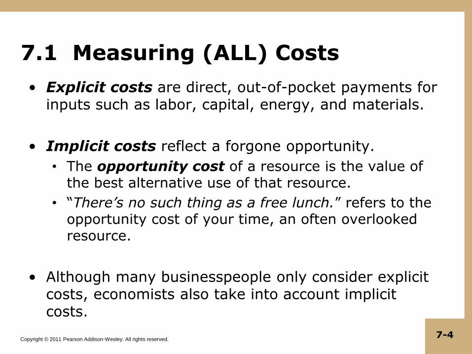
• Explicit costs are direct, out-of-pocket payments for inputs such as labor, capital, energy, and materials.
• Implicit costs reflect a forgone opportunity.
• The opportunity cost of a resource is the value of the best alternative use of that resource.
• “There’s no such thing as a free lunch.” refers to the opportunity cost of your time, an often overlooked resource.
• Although many businesspeople only consider explicit costs, economists also take into account implicit costs.
Copyright © 2011 Pearson Addison-Wesley. All rights reserved. 7-5
7.1 Measuring (ALL) Costs
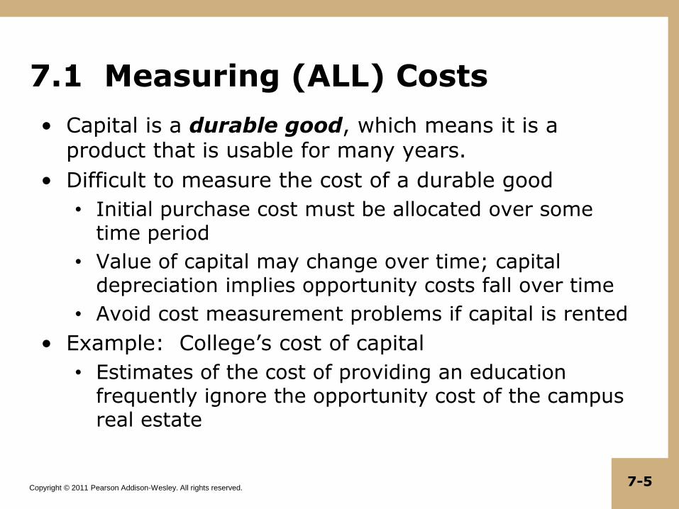
• Capital is a durable good, which means it is a product that is usable for many years.
• Difficult to measure the cost of a durable good
• Initial purchase cost must be allocated over some time period
• Value of capital may change over time; capital depreciation implies opportunity costs fall over time
• Avoid cost measurement problems if capital is rented
• Example: College’s cost of capital
• Estimates of the cost of providing an education frequently ignore the opportunity cost of the campus real estate
Copyright © 2011 Pearson Addison-Wesley. All rights reserved. 7-6
7.1 Measuring (ALL) Costs
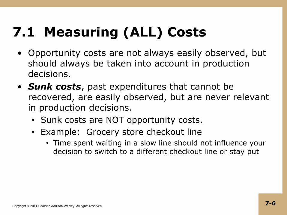
• Opportunity costs are not always easily observed, but should always be taken into account in production decisions.
• Sunk costs, past expenditures that cannot be recovered, are easily observed, but are never relevant in production decisions.
• Sunk costs are NOT opportunity costs.
• Example: Grocery store checkout line
• Time spent waiting in a slow line should not influence your decision to switch to a different checkout line or stay put
Copyright © 2011 Pearson Addison-Wesley. All rights reserved. 7-7
7.2 Short-Run Costs
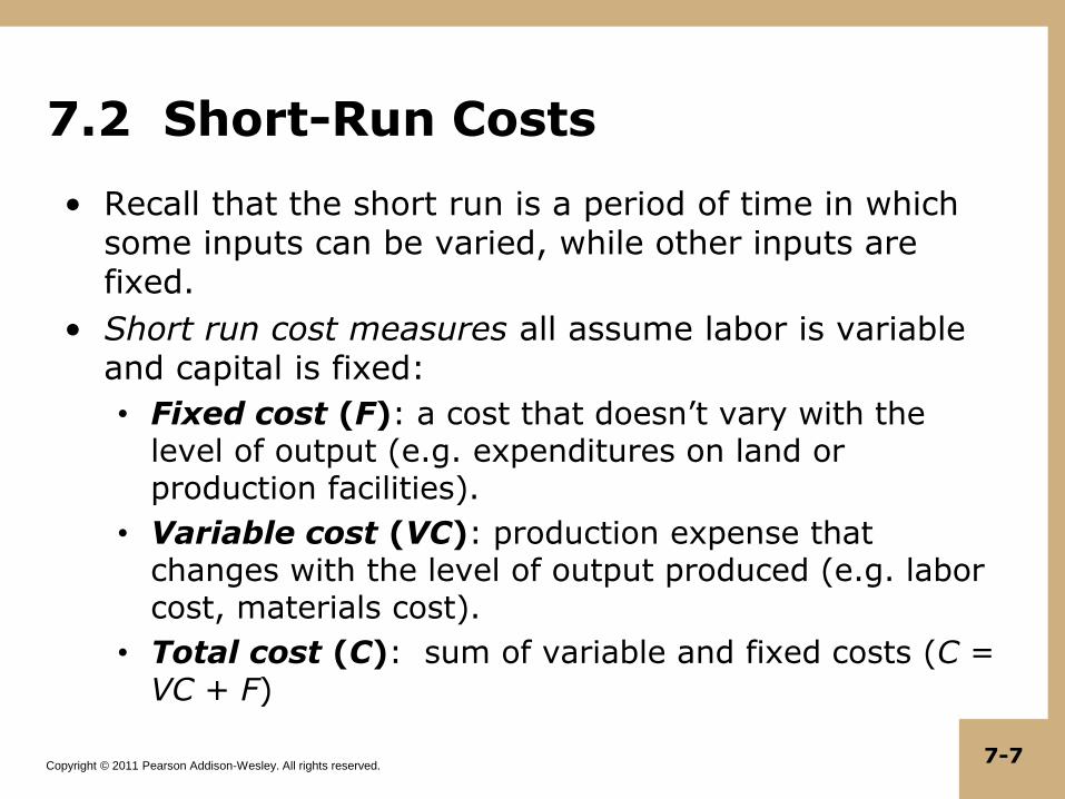
• Recall that the short run is a period of time in which some inputs can be varied, while other inputs are fixed.
• Short run cost measures all assume labor is variable and capital is fixed:
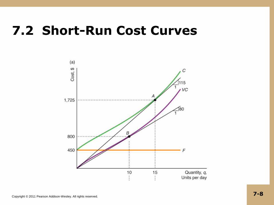
• Fixed cost (F): a cost that doesn’t vary with the level of output (e.g. expenditures on land or production facilities).
• Variable cost (VC): production expense that changes with the level of output produced (e.g. labor cost, materials cost).
• Total cost (C): sum of variable and fixed costs (C = VC + F)
Copyright © 2011 Pearson Addison-Wesley. All rights reserved. 7-8
7.2 Short-Run Cost Curves
Copyright © 2011 Pearson Addison-Wesley. All rights reserved. 7-9
7.2 Short-Run Costs
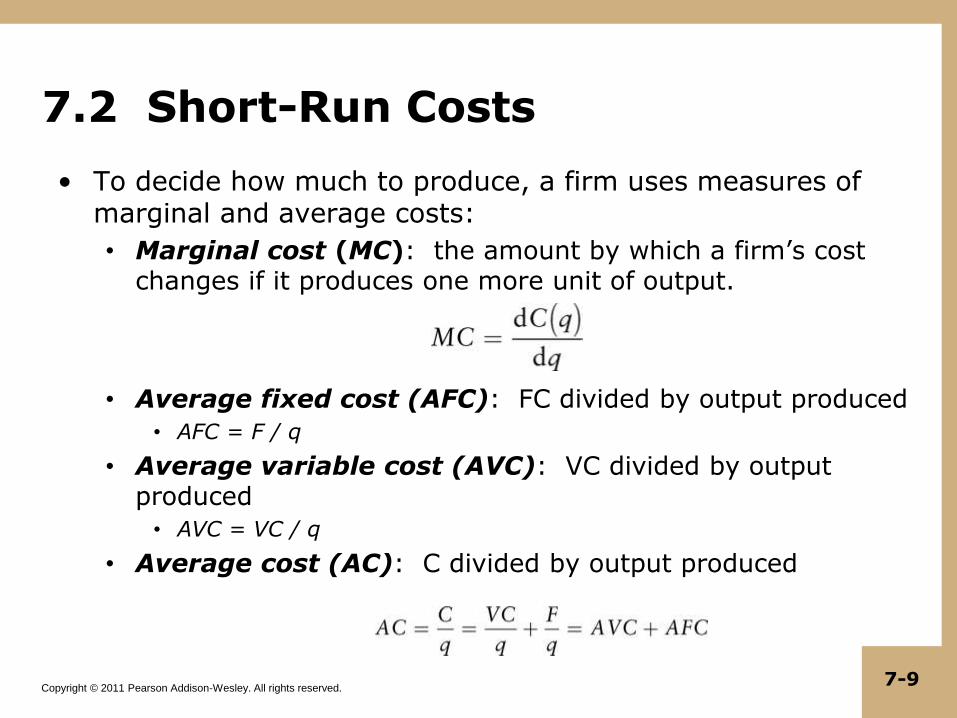
• To decide how much to produce, a firm uses measures of marginal and average costs:
• Marginal cost (MC): the amount by which a firm’s cost changes if it produces one more unit of output.
• Average fixed cost (AFC): FC divided by output produced
• AFC = F / q
• Average variable cost (AVC): VC divided by output produced
• AVC = VC / q
• Average cost (AC): C divided by output produced
Copyright © 2011 Pearson Addison-Wesley. All rights reserved. 7-10
7.2 Short-Run Cost Curves
Copyright © 2011 Pearson Addison-Wesley. All rights reserved. 7-11
7.2 Production Functions and the Shape of Cost Curves
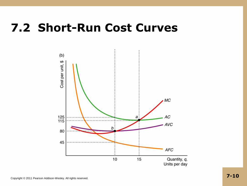
• The SR production function, , determines the shape of a firm’s cost curves.
• We can write q = g(L) because capital is fixed in the SR
• Amount of L needed to produce q is L = g-1(q)
• If the wage paid to labor is w and labor is the only variable input, then variable cost is VC = wL.
• VC is a function of output: V(q) = wL = w g-1(q)
• Total cost is also a function of output:
• C(q) = V(q) + F = w g-1(q) + F
KLfq ,
Copyright © 2011 Pearson Addison-Wesley. All rights reserved. 7-12
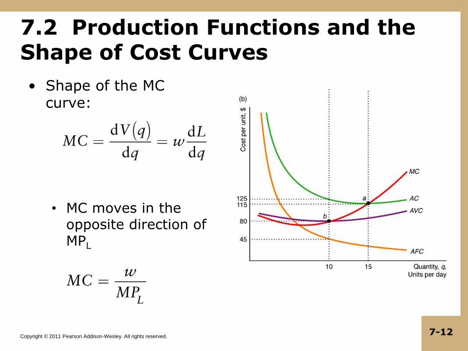
7.2 Production Functions and the Shape of Cost Curves
• Shape of the MC curve:
• MC moves in the opposite direction of MPL
Copyright © 2011 Pearson Addison-Wesley. All rights reserved. 7-13
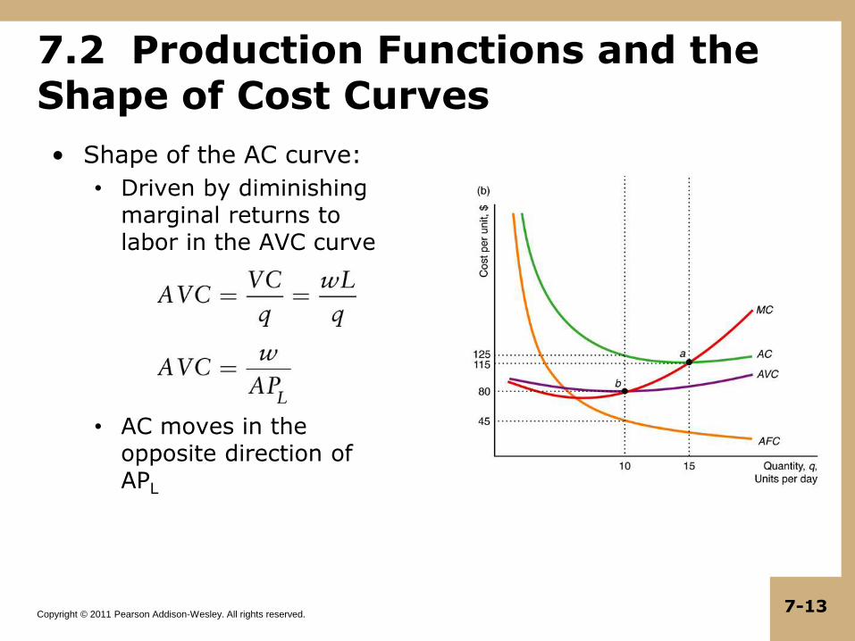
7.2 Production Functions and the Shape of Cost Curves
• Shape of the AC curve:
• Driven by diminishing marginal returns to labor in the AVC curve
• AC moves in the opposite direction of APL
Copyright © 2011 Pearson Addison-Wesley. All rights reserved. 7-14
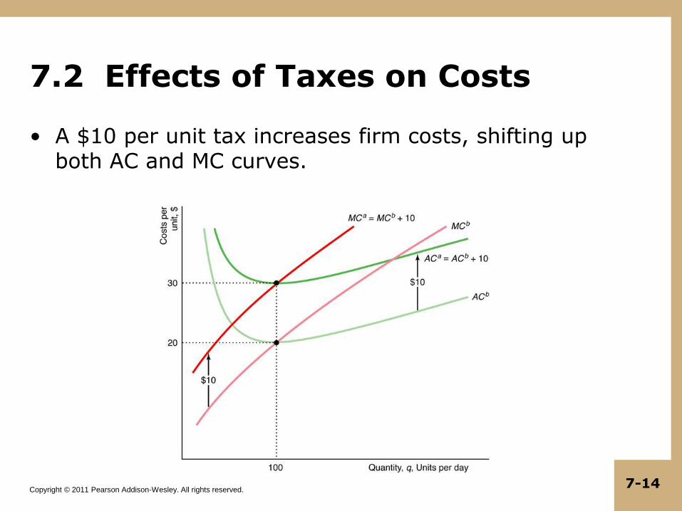
7.2 Effects of Taxes on Costs
• A $10 per unit tax increases firm costs, shifting up both AC and MC curves.
Copyright © 2011 Pearson Addison-Wesley. All rights reserved. 7-15
7.2 Short-Run Cost Summary
• Costs of inputs that can’t be adjusted are fixed and costs of inputs that can be adjusted are variable.
• Shapes of SR cost curves (VC, MC, AC) are determined by the production function.
• When a variable input has diminishing marginal returns, VC and C become steep as output increases.
• Thus, AC, AVC, and MC curves rise with output.
• When MC lies below AVC and AC, it pulls both down; when MC lies above AVC and AC, it pulls both up.
• MC intersects AVC and AC at their minimum points.
Copyright © 2011 Pearson Addison-Wesley. All rights reserved. 7-16
7.3 Long-Run Costs
• Recall that the long run is a period of time in which all inputs can be varied.
• In the LR, firms can change plant size, build new equipment, and adjust inputs that were fixed in the SR.
• We assume LR fixed costs are zero (F = 0).
• In LR, firm concentrates on C, AC, and MC when it decides how much labor (L) and capital (K) to employ in the production process.
Copyright © 2011 Pearson Addison-Wesley. All rights reserved. 7-17
7.3 Long-Run Costs and Input Choice
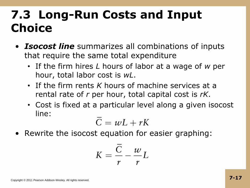
• Isocost line summarizes all combinations of inputs that require the same total expenditure
• If the firm hires L hours of labor at a wage of w per hour, total labor cost is wL.
• If the firm rents K hours of machine services at a rental rate of r per hour, total capital cost is rK.
• Cost is fixed at a particular level along a given isocost line:
• Rewrite the isocost equation for easier graphing:
Copyright © 2011 Pearson Addison-Wesley. All rights reserved. 7-18
7.3 Isocost Lines
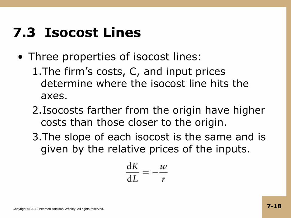
• Three properties of isocost lines:
1.The firm’s costs, C, and input prices determine where the isocost line hits the axes.
2.Isocosts farther from the origin have higher costs than those closer to the origin.
3.The slope of each isocost is the same and is given by the relative prices of the inputs.
Copyright © 2011 Pearson Addison-Wesley. All rights reserved. 7-19
7.3 Cost Minimization
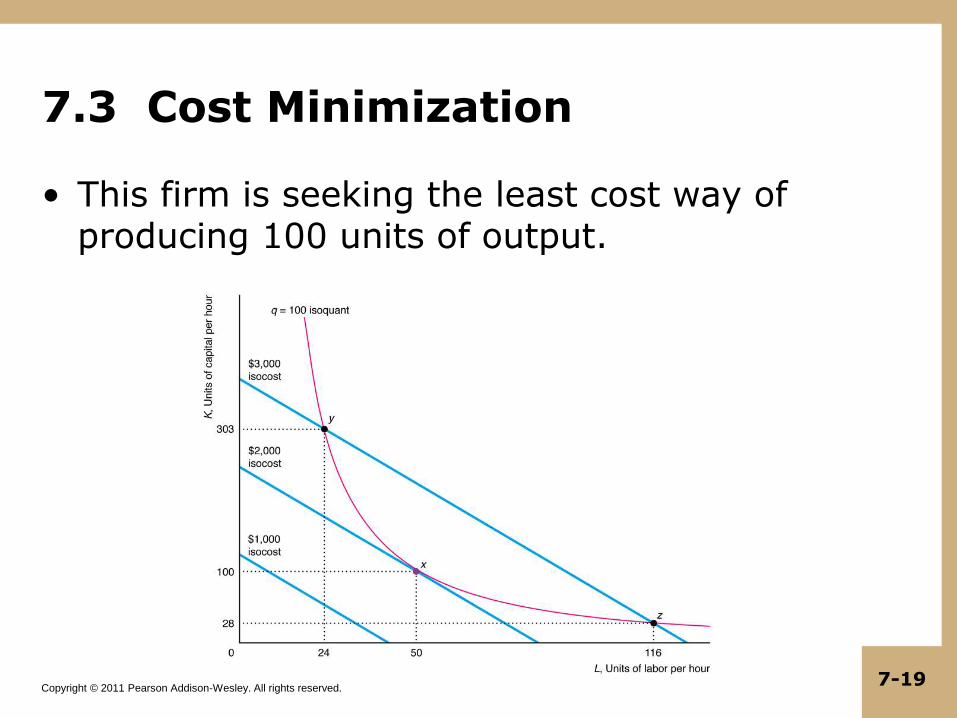
• This firm is seeking the least cost way of producing 100 units of output.
Copyright © 2011 Pearson Addison-Wesley. All rights reserved. 7-20
7.3 Cost Minimization
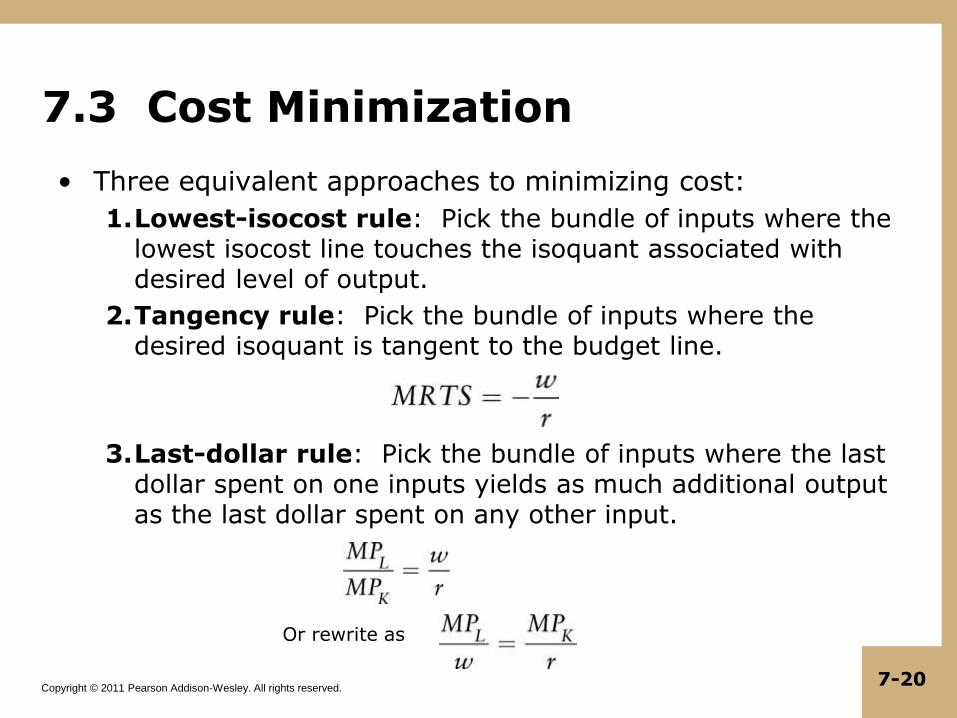
• Three equivalent approaches to minimizing cost:
1.Lowest-isocost rule: Pick the bundle of inputs where the lowest isocost line touches the isoquant associated with desired level of output.
2.Tangency rule: Pick the bundle of inputs where the desired isoquant is tangent to the budget line.
3.Last-dollar rule: Pick the bundle of inputs where the last dollar spent on one inputs yields as much additional output as the last dollar spent on any other input.
Or rewrite as
Copyright © 2011 Pearson Addison-Wesley. All rights reserved. 7-21
7.3 Cost Minimization with Calculus
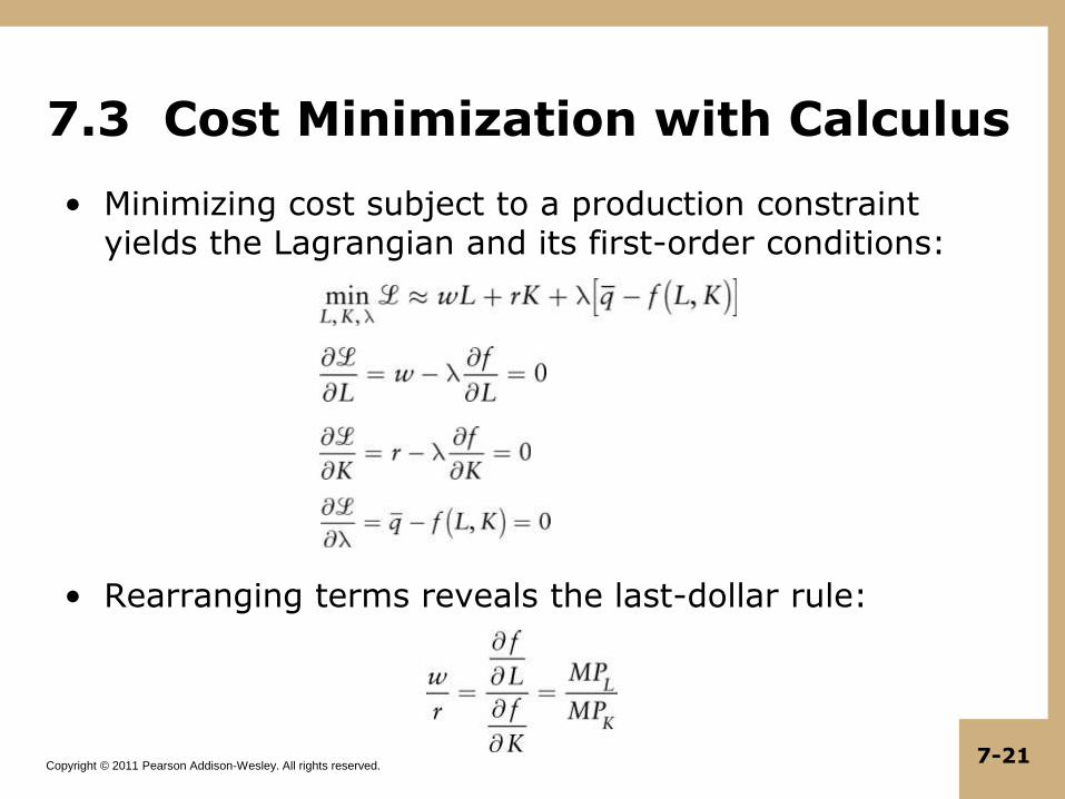
• Minimizing cost subject to a production constraint yields the Lagrangian and its first-order conditions:
• Rearranging terms reveals the last-dollar rule:
Copyright © 2011 Pearson Addison-Wesley. All rights reserved. 7-22
7.3 Output Maximization with Calculus
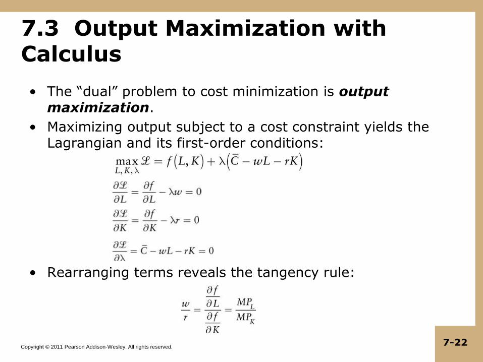
• The “dual” problem to cost minimization is output maximization.
• Maximizing output subject to a cost constraint yields the Lagrangian and its first-order conditions:
• Rearranging terms reveals the tangency rule:
Copyright © 2011 Pearson Addison-Wesley. All rights reserved. 7-23
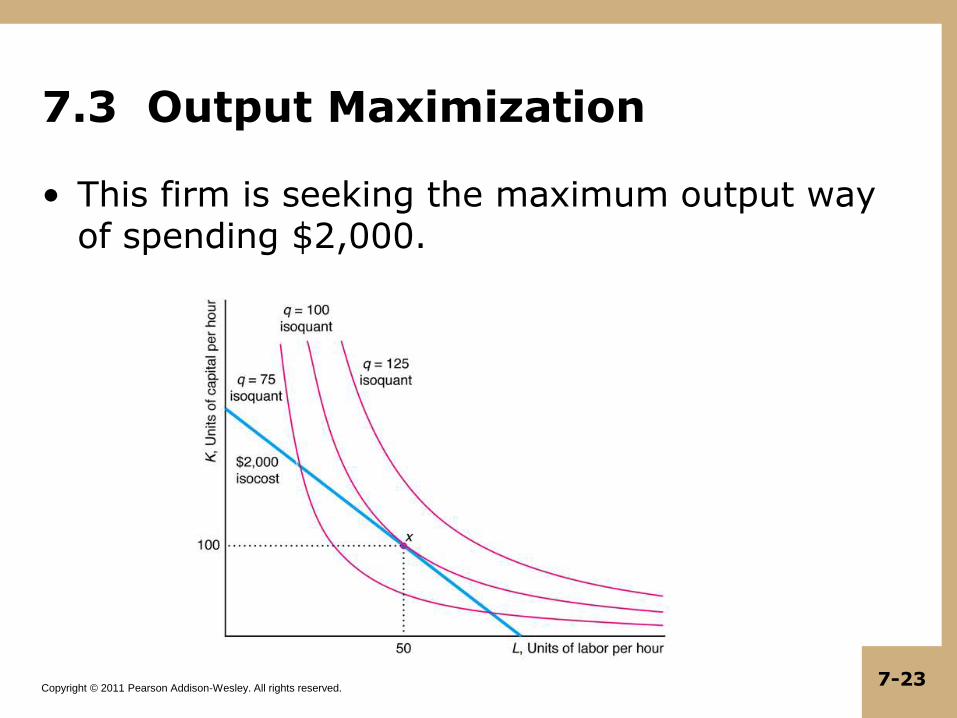
7.3 Output Maximization
• This firm is seeking the maximum output way of spending $2,000.
Copyright © 2011 Pearson Addison-Wesley. All rights reserved. 7-24
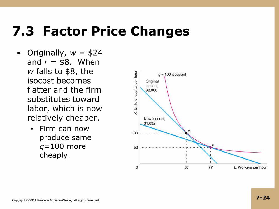
7.3 Factor Price Changes
• Originally, w = $24 and r = $8. When w falls to $8, the isocost becomes flatter and the firm substitutes toward labor, which is now relatively cheaper.
• Firm can now produce same q=100 more cheaply.
Copyright © 2011 Pearson Addison-Wesley. All rights reserved. 7-25
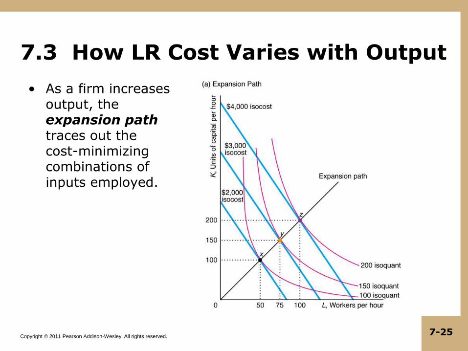
7.3 How LR Cost Varies with Output
• As a firm increases output, the expansion path traces out the cost-minimizing combinations of inputs employed.
Copyright © 2011 Pearson Addison-Wesley. All rights reserved. 7-26
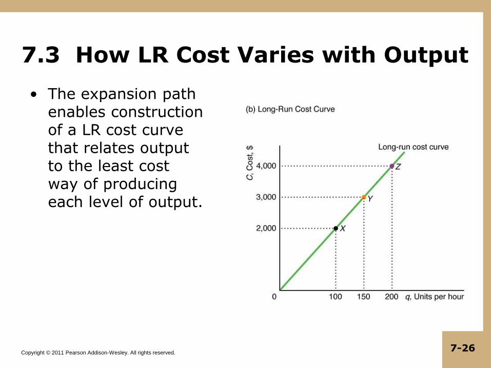
7.3 How LR Cost Varies with Output
• The expansion path enables construction of a LR cost curve that relates output to the least cost way of producing each level of output.
Copyright © 2011 Pearson Addison-Wesley. All rights reserved. 7-27
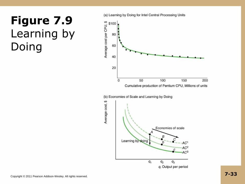
7.3 The Shape of LR Cost Curves
• The LR AC curve may be U-shaped
• Not due to downward-sloping AFC or diminishing marginal returns, both of which are SR phenomena, as it is for SR AC.
• Shape is due to economies and diseconomies of scale.
• A cost function exhibits economies of scale if the average cost of production falls as output expands.
• Doubling inputs more than doubles output, so AC falls with higher output.
• A cost function exhibits diseconomies of scale if the average cost of production rises as output expands.
• Doubling inputs less than doubles output, so AC rises with higher output.
Copyright © 2011 Pearson Addison-Wesley. All rights reserved. 7-28
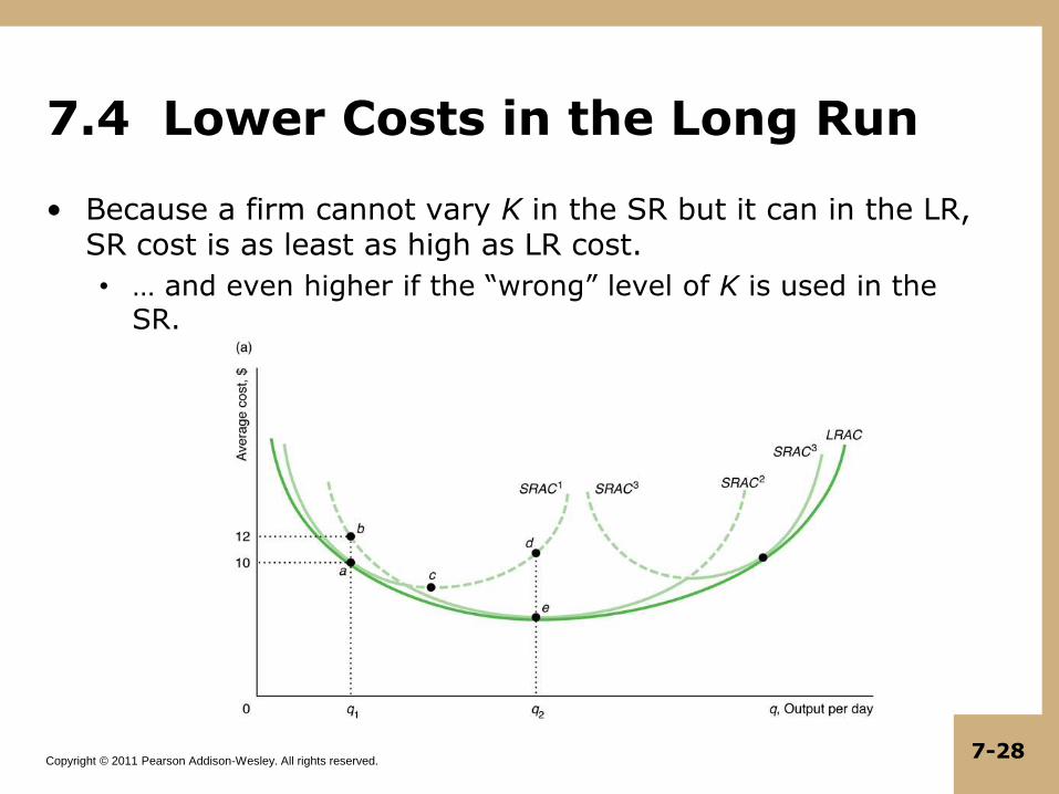
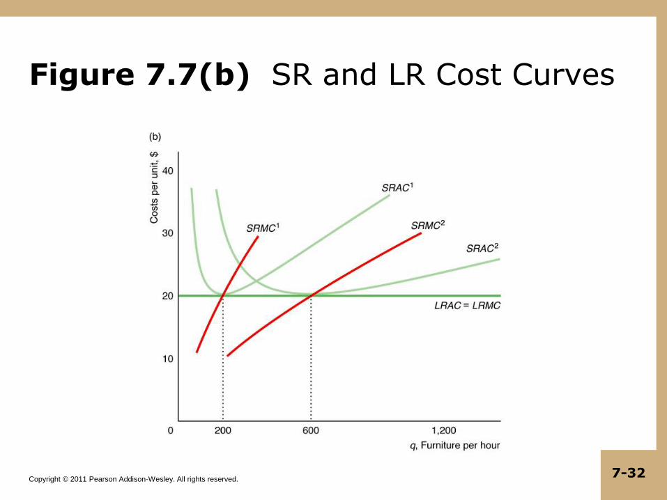
7.4 Lower Costs in the Long Run
• Because a firm cannot vary K in the SR but it can in the LR, SR cost is as least as high as LR cost.
• … and even higher if the “wrong” level of K is used in the SR.
Copyright © 2011 Pearson Addison-Wesley. All rights reserved. 7-29
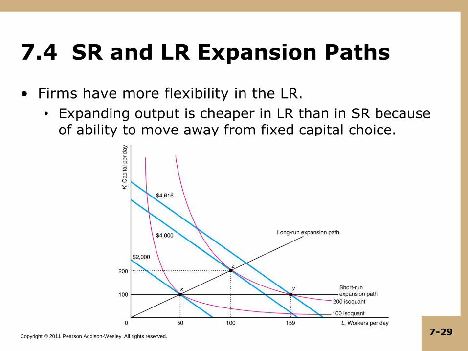
7.4 SR and LR Expansion Paths
• Firms have more flexibility in the LR.
• Expanding output is cheaper in LR than in SR because of ability to move away from fixed capital choice.
Copyright © 2011 Pearson Addison-Wesley. All rights reserved. 7-30
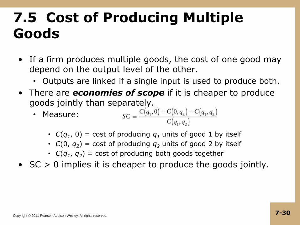
7.5 Cost of Producing Multiple Goods
• If a firm produces multiple goods, the cost of one good may depend on the output level of the other.
• Outputs are linked if a single input is used to produce both.
• There are economies of scope if it is cheaper to produce goods jointly than separately.
• Measure:
• C(q1, 0) = cost of producing q1 units of good 1 by itself
• C(0, q2) = cost of producing q2 units of good 2 by itself
• C(q1, q2) = cost of producing both goods together
• SC > 0 implies it is cheaper to produce the goods jointly.
Copyright © 2011 Pearson Addison-Wesley. All rights reserved. 7-31
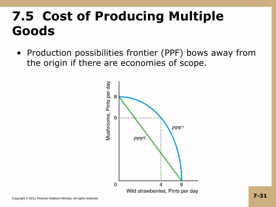
7.5 Cost of Producing Multiple Goods
• Production possibilities frontier (PPF) bows away from the origin if there are economies of scope.
Copyright © 2011 Pearson Addison-Wesley. All rights reserved. 7-32
Figure 7.7(b) SR and LR Cost Curves
Copyright © 2011 Pearson Addison-Wesley. All rights reserved. 7-33
Figure 7.9 Learning by Doing