Chapter 7 Spatial Domain Image Transforms - CEE Cornellceeserver.cee.cornell.edu/wdp2/cee6150/Text-Richard... · Chapter 7 Spatial Domain Image Transforms 7.1 Introduction In the

Chapter 7Spatial Domain Image Transforms

7.1 Introduction

In the material presented in Chap. 5 we looked at a number of geometricprocessing operations that involve the spatial properties of an image. Averagingover adjacent groups of pixels to reduce noise, and looking at local spatialgradients to enhance edge and line features, are examples. There are, however,more sophisticated approaches for processing the spatial domain properties of animage. The most recognisable is probably the Fourier transformation which weconsider in this chapter, allowing us to understand what are called the spatialfrequency components of an image. Once we can use the Fourier transformationwe will see that it offers a powerful method for generating the sorts of operationwe did with templates in Chap. 5.

There are other spatial transformation techniques as well. Some we willmention in passing that find application in image compression in the video andtelevision industry. More recent techniques, such as the wavelet transform, haveemerged as important image processing tools in their own right, including inremote sensing. The wavelet transform is introduced later in this chapter.

We commence with some necessary mathematical background that leads, in thefirst instance, to the principles of sampling theory. That is sampling, not inthe statistical sense that we use when testing map accuracy in Chap. 11, but in therole of digitising a continuous landscape to produce an image composed of discretepixels. This material is based on two mathematical fields that the earth sciencereader may not have encountered in the past: the first is complex numbers and thesecond is integral calculus. We will work our way through that material as care-fully as possible but for those readers not needing a background on transformationmethods, this chapter can be passed over without affecting an understanding of theremainder of the book.

J. A. Richards, Remote Sensing Digital Image Analysis,DOI: 10.1007/978-3-642-30062-2_7, � Springer-Verlag Berlin Heidelberg 2013

203

http://dx.doi.org/10.1007/978-3-642-30062-2_5

http://dx.doi.org/10.1007/978-3-642-30062-2_5

http://dx.doi.org/10.1007/978-3-642-30062-2_5

http://dx.doi.org/10.1007/978-3-642-30062-2_5

http://dx.doi.org/10.1007/978-3-642-30062-2_11

http://dx.doi.org/10.1007/978-3-642-30062-2_11

7.2 Special Functions

Three special functions are important in understanding the development ofsampling theory and the transformations treated here. We will consider them asfunctions of time, because that is the way most are presented in classical texts, butthey will be interpreted as functions of position, in either one or two dimensions asrequired, later in the chapter.

7.2.1 The Complex Exponential Function

Several of the functions we meet here involve imaginary numbers which arisewhen we try to take the square root of a negative number. The most basic is thesquare root of �1: Although that may seem to be an unusual concept, it is anenormously valuable mathematical construct in developing transformations. It issufficient here to consider

ffiffiffiffiffiffiffi

�1p

as a special symbol rather than try to understandthe logical implications of taking the square root of something that is negative. It isgiven the symbol j in the engineering literature, but is represented by i in themathematical literature.

By definition, a complex exponential function1 that is periodic with time is

g tð Þ ¼ ejxt ð7:1Þ

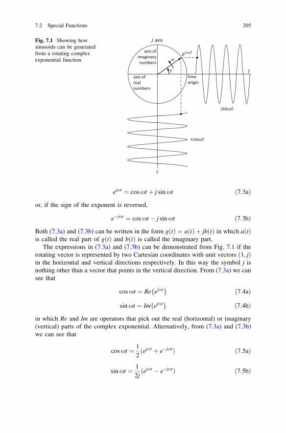
This is best looked at as a vector that rotates in an anticlockwise direction in atwo-dimensional plane (called an Argand diagram) described by real and imaginarynumber axes as shown in Fig. 7.1. The concept of an imaginary number isdeveloped below. If the exponent in (7.1) were negative the vector would rotate inthe clockwise direction. As the vector rotates from its position at time zero itsprojection onto the axis of real numbers plots out the cosine function whereas itsprojection onto the axis of imaginary numbers plots out the sine function. Onecomplete rotation of the vector, covering 360� or 2p radians, takes place in a timet ¼ T defined by xT ¼ 2p: T ¼ 2p=x is called the period of the function,measured in seconds, and x is called its radian frequency, with units of radians persecond. Note, for example, if the period is 10 ms, the radian frequency would be200p ¼ 628 rad s�1: Often we describe frequency f in hertz rather than as x inradians per second. The two measures are related by

x ¼ 2pf ð7:2Þ

The complex exponential expression in (7.1) can be written2

1 We use the symbol g here for a general function, rather than the more usual f ; to avoidconfusion with the symbol universally used for frequency.2 This is known as Euler’s theorem.

204 7 Spatial Domain Image Transforms

ejxt ¼ cos xt þ j sin xt ð7:3aÞ

or, if the sign of the exponent is reversed,

e�jxt ¼ cos xt � j sin xt ð7:3bÞ

Both (7.3a) and (7.3b) can be written in the form g tð Þ ¼ a tð Þ þ jbðtÞ in which a tð Þis called the real part of g tð Þ and bðtÞ is called the imaginary part.

The expressions in (7.3a) and (7.3b) can be demonstrated from Fig. 7.1 if therotating vector is represented by two Cartesian coordinates with unit vectors ð1; jÞin the horizontal and vertical directions respectively. In this way the symbol j isnothing other than a vector that points in the vertical direction. From (7.3a) we cansee that

cos xt ¼ Refejxtg ð7:4aÞ

sin xt ¼ Imfejxtg ð7:4bÞ

in which Re and Im are operators that pick out the real (horizontal) or imaginary(vertical) parts of the complex exponential. Alternatively, from (7.3a) and (7.3b)we can see that

cos xt ¼ 12ðejxt þ e�jxtÞ ð7:5aÞ

sin xt ¼ 12jðejxt � e�jxtÞ ð7:5bÞ

Fig. 7.1 Showing howsinusoids can be generatedfrom a rotating complexexponential function

7.2 Special Functions 205

7.2.2 The Impulse or Delta Function

An important function for understanding the properties of sampled signals,including digital image data, is the impulse function. It is also referred to as theDirac delta function, or simply the delta function. It is spike-like, of infiniteamplitude and infinitesimal duration. It cannot be defined explicitly. Instead, it isdescribed by a limiting operation in the following manner.

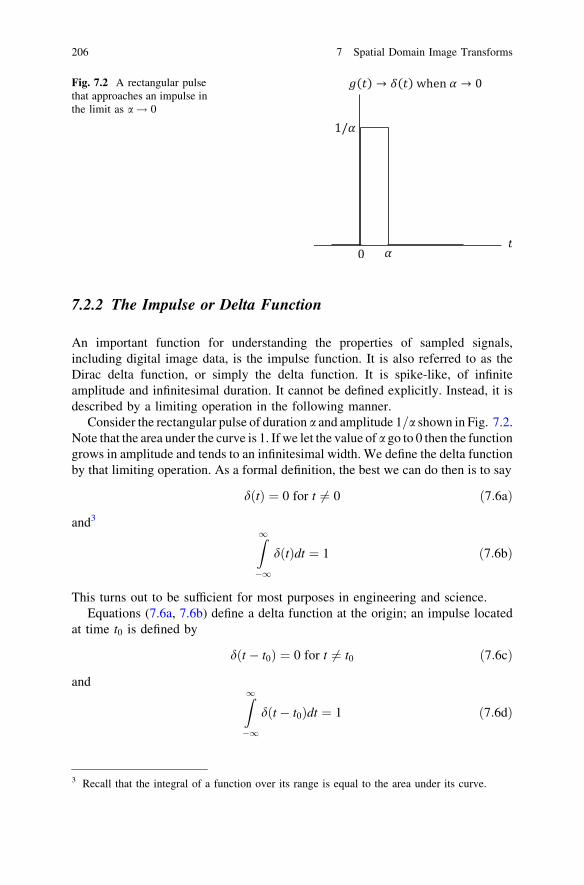
Consider the rectangular pulse of duration a and amplitude 1=a shown in Fig. 7.2.Note that the area under the curve is 1. If we let the value of a go to 0 then the functiongrows in amplitude and tends to an infinitesimal width. We define the delta functionby that limiting operation. As a formal definition, the best we can do then is to say

dðtÞ ¼ 0 for t 6¼ 0 ð7:6aÞ

and3

Z

1

�1

dðtÞdt ¼ 1 ð7:6bÞ

This turns out to be sufficient for most purposes in engineering and science.Equations (7.6a, 7.6b) define a delta function at the origin; an impulse located

at time t0 is defined by

dðt � t0Þ ¼ 0 for t 6¼ t0 ð7:6cÞ

andZ

1

�1

dðt � t0Þdt ¼ 1 ð7:6dÞ

Fig. 7.2 A rectangular pulsethat approaches an impulse inthe limit as a! 0

3 Recall that the integral of a function over its range is equal to the area under its curve.


If we take the product of a delta function with another function the result, from(7.6c), is

d t � t0ð Þg tð Þ ¼ d t � t0ð Þg t0ð Þ ð7:7Þ

From this we see

Z

1

�1

d t � t0ð Þg tð Þdt ¼Z

1

�1

d t � t0ð Þg t0ð Þdt ¼ g t0ð ÞZ

1

�1

d t � t0ð Þdt ¼ g t0ð Þ ð7:8Þ

This is known as the sifting property of the impulse.

7.2.3 The Heaviside Step Function

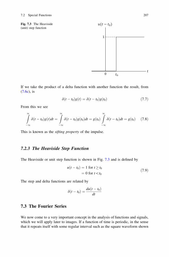
The Heaviside or unit step function is shown in Fig. 7.3 and is defined by

u t � t0ð Þ ¼ 1 for t� t0

¼ 0 for t\t0ð7:9Þ

The step and delta functions are related by

d t � t0ð Þ ¼ duðt � t0Þdt

7.3 The Fourier Series

We now come to a very important concept in the analysis of functions and signals,which we will apply later to images. If a function of time is periodic, in the sensethat it repeats itself with some regular interval such as the square waveform shown

Fig. 7.3 The Heaviside(unit) step function

7.2 Special Functions 207

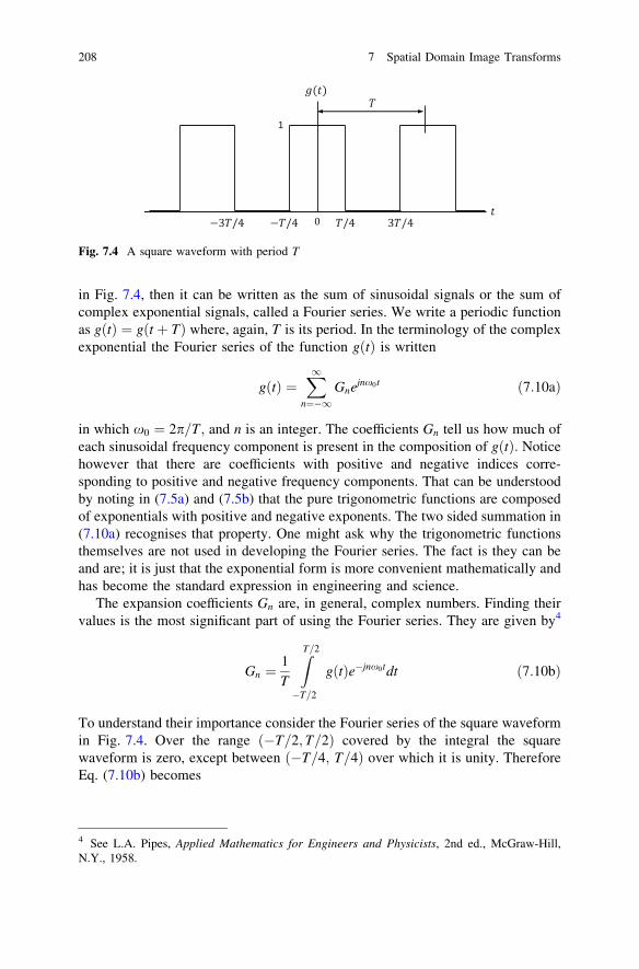
in Fig. 7.4, then it can be written as the sum of sinusoidal signals or the sum ofcomplex exponential signals, called a Fourier series. We write a periodic functionas g tð Þ ¼ gðt þ TÞ where, again, T is its period. In the terminology of the complexexponential the Fourier series of the function gðtÞ is written

g tð Þ ¼X

1

n¼�1Gnejnx0t ð7:10aÞ

in which x0 ¼ 2p=T; and n is an integer. The coefficients Gn tell us how much ofeach sinusoidal frequency component is present in the composition of gðtÞ: Noticehowever that there are coefficients with positive and negative indices corre-sponding to positive and negative frequency components. That can be understoodby noting in (7.5a) and (7.5b) that the pure trigonometric functions are composedof exponentials with positive and negative exponents. The two sided summation in(7.10a) recognises that property. One might ask why the trigonometric functionsthemselves are not used in developing the Fourier series. The fact is they can beand are; it is just that the exponential form is more convenient mathematically andhas become the standard expression in engineering and science.

The expansion coefficients Gn are, in general, complex numbers. Finding theirvalues is the most significant part of using the Fourier series. They are given by4

Gn ¼1T

Z

T=2

�T=2

gðtÞe�jnx0tdt ð7:10bÞ

To understand their importance consider the Fourier series of the square waveformin Fig. 7.4. Over the range ð�T=2; T=2Þ covered by the integral the squarewaveform is zero, except between ð�T=4; T=4Þ over which it is unity. ThereforeEq. (7.10b) becomes

Fig. 7.4 A square waveform with period T

4 See L.A. Pipes, Applied Mathematics for Engineers and Physicists, 2nd ed., McGraw-Hill,N.Y., 1958.


Gn ¼1T

Z

T=4

�T=4

e�jnx0tdt ¼ 1np

sinnp2

The first few values of this last expression for positive and negative values of n are

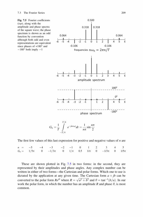
These are shown plotted in Fig. 7.5 in two forms: in the second, they arerepresented by their amplitudes and phase angles. Any complex number can bewritten in either of two forms—the Cartesian and polar forms. Which one to use isdictated by the application at any given time. The Cartesian form aþ jb can be

converted to the polar form Rejh where R ¼ffiffiffiffiffiffiffiffiffiffiffiffiffiffiffi

a2 þ b2p

and h ¼ tan�1ðb=aÞ: In ourwork the polar form, in which the number has an amplitude R and phase h, is mostcommon.

Fig. 7.5 Fourier coefficients(top), along with theamplitude and phase spectraof the square wave; the phasespectrum is shown as an oddfunction by conventionalthough both odd and evenrepresentations are equivalentsince phases of +180� and-180� both imply -1

n ¼ -5 -4 -3 -2 -1 0 1 2 3 4 5Gn ¼ 1=5p 0 �1=3p 0 1=p 0.5 1/p 0 -1/3p 0 1/5p

7.3 The Fourier Series 209

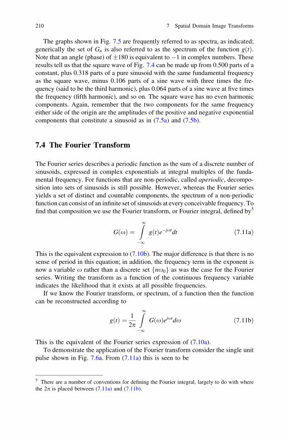
The graphs shown in Fig. 7.5 are frequently referred to as spectra, as indicated;generically the set of Gn is also referred to as the spectrum of the function gðtÞ:Note that an angle (phase) of �180 is equivalent to �1 in complex numbers. Theseresults tell us that the square wave of Fig. 7.4 can be made up from 0.500 parts of aconstant, plus 0.318 parts of a pure sinusoid with the same fundamental frequencyas the square wave, minus 0.106 parts of a sine wave with three times the fre-quency (said to be the third harmonic), plus 0.064 parts of a sine wave at five timesthe frequency (fifth harmonic), and so on. The square wave has no even harmoniccomponents. Again, remember that the two components for the same frequencyeither side of the origin are the amplitudes of the positive and negative exponentialcomponents that constitute a sinusoid as in (7.5a) and (7.5b).

7.4 The Fourier Transform

The Fourier series describes a periodic function as the sum of a discrete number ofsinusoids, expressed in complex exponentials at integral multiples of the funda-mental frequency. For functions that are non-periodic, called aperiodic, decompo-sition into sets of sinusoids is still possible. However, whereas the Fourier seriesyields a set of distinct and countable components, the spectrum of a non-periodicfunction can consist of an infinite set of sinusoids at every conceivable frequency. Tofind that composition we use the Fourier transform, or Fourier integral, defined by5

GðxÞ ¼Z

1

�1

gðtÞe�jxtdt ð7:11aÞ

This is the equivalent expression to (7.10b). The major difference is that there is nosense of period in this equation; in addition, the frequency term in the exponent isnow a variable x rather than a discrete set fnx0g as was the case for the Fourierseries. Writing the transform as a function of the continuous frequency variableindicates the likelihood that it exists at all possible frequencies.

If we know the Fourier transform, or spectrum, of a function then the functioncan be reconstructed according to

gðtÞ ¼ 12p

Z

1

�1

GðxÞejxtdx ð7:11bÞ

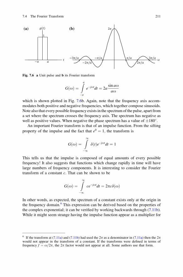
This is the equivalent of the Fourier series expression of (7.10a).To demonstrate the application of the Fourier transform consider the single unit

pulse shown in Fig. 7.6a. From (7.11a) this is seen to be

5 There are a number of conventions for defining the Fourier integral, largely to do with wherethe 2p is placed between (7.11a) and (7.11b).


G xð Þ ¼Z

a

�a

e�jxtdt ¼ 2asin ax

ax

which is shown plotted in Fig. 7.6b. Again, note that the frequency axis accom-modates both positive and negative frequencies, which together compose sinusoids.Note also that every possible frequency exists in the spectrum of the pulse, apart froma set where the spectrum crosses the frequency axis. The spectrum has negative aswell as positive values. When negative the phase spectrum has a value of �180�:

An important Fourier transform is that of an impulse function. From the siftingproperty of the impulse and the fact that e0 ¼ 1; the transform is

G xð Þ ¼Z

1

�1

dðtÞe�jxtdt ¼ 1

This tells us that the impulse is composed of equal amounts of every possiblefrequency! It also suggests that functions which change rapidly in time will havelarge numbers of frequency components. It is interesting to consider the Fouriertransform of a constant c. That can be shown to be

G xð Þ ¼Z

1

�1

ce�jxtdt ¼ 2pcdðxÞ

In other words, as expected, the spectrum of a constant exists only at the origin inthe frequency domain.6 This expression can be derived based on the properties ofthe complex exponential; it can be verified by working backwards through (7.11b).While it might seem strange having the impulse function appear as a multiplier for

(a) (b)

Fig. 7.6 a Unit pulse and b its Fourier transform

6 If the transform at (7.11a) and (7.11b) had used the 2p as a denominator in (7.11a) then the 2pwould not appear in the transform of a constant. If the transforms were defined in terms offrequency f ¼ x=2p; the 2p factor would not appear at all. Some authors use that form.

7.4 The Fourier Transform 211

the constant, we can safely interpret that as just a reminder that the constant existsat x ¼ 0 and not as something that changes the amplitude of the constant.

The Fourier transform of a periodic function, normally expressed using the Fourierseries, is important. We can obtain it by substituting (7.10a) into (7.11a) to give

G xð Þ ¼Z

1

�1

X

1

n¼�1Gnejnx0te�jxtdt

i.e. G xð Þ ¼X

1

n¼�1Gn

Z

1

�1

ej nx0�xð Þtdt

which becomes G xð Þ ¼ 2pX

1

n¼�1Gndðx� nx0Þ ð7:12Þ

This last expression uses the property for the Fourier transform of a constant (inthis case unity). It tells us that the only frequencies that can exist in the Fouriertransform of a periodic function are those which are integral multiples of thefundamental frequency of the periodic waveform.

The last example is important because it tells us that we do not need to workwith both Fourier series and Fourier transforms. Because the Fourier transformalso applies to periodic functions, it is sufficient in the following to focus on thetransform alone.

7.5 The Discrete Fourier Transform

Because our interest is in digital imagery, which is simply a two-dimensionalversion of the one-dimensional functions we have been considering up to now, it isimportant to move away from continuous functions of time (or any other inde-pendent variable) and instead look at the situation when the independent variableis discrete, and the dependent variable consists of a set of samples.

Suppose we have a set of K samples over a time interval T of the continuousfunction gðtÞ. Call these samples c kð Þ; k ¼ 0. . .K � 1: The individual samplesoccur at the times tk ¼ kDt where Dt is the spacing between samples. Note thatT ¼ KDt: Consider now how (7.11a) needs to be modified to handle the set ofsamples rather than a continuous function of time. First, obviously the functionitself is replaced by the samples. Secondly the integral over time is replaced by thesum over the samples and the infinitesimal time increment dt in the integral isreplaced by the sampling time increment Dt: The time variable t is replaced bykDt ¼ kT

K ; k ¼ 0. . .K � 1: So far this gives as a discrete form of (7.11a)


GðxÞ ¼ DtX

K�1

k¼0

c kð Þe�jxkDt

We now have to consider how to treat the frequency variable x: We are developingthis discrete form of the Fourier transformation so that it can handle digitised dataand so that it can be processed by computer. Therefore, the frequency domain alsohas to be digitised by replacing x by the frequency samples x ¼ rDx;r ¼ 0. . .K � 1:We have deliberately chosen the number of samples in the frequencydomain to be the same as the number in the time domain for convenience. Whatvalue now do we give to the increment in frequency Dx? That is not easily answereduntil we have treated sampling theory later in this chapter, so for the present note thatit will be 2p=T and thus is directly related to the time over which the originalfunction has been sampled. With this treatment of the frequency variable the lastexpression for the discrete version of the Fourier transform now becomes

G rð Þ ¼ DtX

K�1

k¼0

c kð Þe�j2prk

K r ¼ 0. . .K � 1

It is common to define W ¼ e�j2p=K ð7:13Þ

so that the last expression is written

G rð Þ ¼ DtX

K�1

k¼0

c kð ÞWrk r ¼ 0. . .K � 1 ð7:14aÞ

Equation (7.14a) is known as the discrete Fourier transform (DFT). In a similarmanner we can derive a discrete inverse Fourier transform (IDFT) to allow theoriginal sequence c kð Þ to be reconstructed from the frequency samples GðrÞ: That isgiven by

cðkÞ ¼ 1T

X

K�1

r¼0

G rð ÞW�rk k ¼ 0. . .K � 1 ð7:14bÞ

If we substitute (7.14a) into (7.14b) we see they do in fact constitute a transform pair.To do so we need different indices for k; we will use l instead of k in (7.14b) so that

cðlÞ ¼ 1T

X

K�1

r¼0

G rð ÞW�rl ¼ 1T

X

K�1

r¼0

DtX

K�1

k¼0

c kð ÞWrkW�rl

i.e.

cðlÞ ¼ 1K

X

K�1

k¼0

c kð ÞX

K�1

r¼0

Wrðk�lÞ

7.5 The Discrete Fourier Transform 213

From the properties of the complex exponential function the second sum is zero fork 6¼ l and is K when k ¼ l; so that the right hand side becomes cðlÞ as required.An interesting by-product of this analysis has been that the Dt and T divide toleave K; the number of samples. As a result, the transform pair in (7.14a) and(7.14b) can be written in the simpler form, used in software that computes thediscrete Fourier transform:

G rð Þ ¼X

K�1

k¼0

c kð ÞWrk r ¼ 0. . .K � 1 ð7:15aÞ

cðkÞ ¼ 1K

X

K�1

r¼0

G rð ÞW�rk k ¼ 0. . .K � 1 ð7:15bÞ

These last two expressions are particularly simple. All they involve are the sets ofsamples to be transformed (or inverse transformed) and the complex constants W ;which can be computed beforehand.

7.5.1 Properties of the Discrete Fourier Transform

Three properties of the DFT and IDFT are important.

LinearityBoth the DFT and IDFT are linear operations. Thus, if the set G1ðrÞ is the DFT ofthe sequence c1ðkÞ and the set G2ðrÞ is the DFT of the sequence c2ðkÞ then, for anyconstants, a and b; aG1 rð Þ þ bG2ðrÞ is the DFT of ac1 kð Þ þ bc2ðkÞ:

PeriodicityFrom (7.13) W�mkK ¼ 1 where m and k are integers, so that

G r þ mKð Þ ¼X

K�1

k¼0

c kð ÞW ðrþmKÞk ¼ GðrÞ ð7:16aÞ

similarly c k þ mKð Þ ¼ 1K

X

K�1

r¼0

G rð ÞW�r kþmKð Þ ¼ c kð Þ ð7:16bÞ

Thus both the sequence of samples and the set of transformed samples are periodicwith period K. This has two important implications. First, to generate the Fourierseries of a periodic function it is only necessary to sample it over a single period.Secondly, the spectrum of an aperiodic function will be that of a periodic repetitionof that function over the sampling duration—in other words it is made to lookperiodic by the limited time sampling. Therefore, for a limited time function such


as the rectangular pulse shown in Fig. 7.6, it is necessary to sample the signalbeyond the arguments for which it is non-zero so it looks approximately aperiodic.

SymmetryPut r0 ¼ K � r in (7.15a) to give

G r0ð Þ ¼X

K�1

k¼0

c kð ÞW ðK�rÞk

Since WkK ¼ 1 then G K � rð Þ ¼ G�ðrÞ where the * represents the complexconjugate. This implies that the amplitude spectrum is symmetric about K=2 andthe phase spectrum is antisymmetric.

7.5.2 Computing the Discrete Fourier Transform

Evaluating the K values of GðrÞ from the K values of cðkÞ in (7.15a) requires K2

multiplications and K2 additions, assuming that the values of Wrk have beencalculated beforehand. Since those numbers are complex, the multiplications andadditions required to evaluate the Fourier transform are also complex. It is themultiplications that are the problem; complex multiplications require significantcomputing resources, so that transforms involving of the order of 1,000 samplescan take significant time. Fortunately, a fast algorithm, called the fast Fouriertransform (FFT), is available.7 It only requires K

2 log2K complex multiplications,which is a substantial reduction in computational demand. The implementation ofthe DFT in software uses the FFT algorithm. The only penalty in using this methodis that the number of samples taken of the function to be transformed, and thenumber of samples in the transform, each have to be a power of two.

7.6 Convolution

7.6.1 The Convolution Integral

Before proceeding to look at the Fourier transform of an image it is of value toappreciate the operation called convolution. It was introduced in Sect. 5.8 in thecontext of geometric enhancement of imagery. We now look at it in more detailbecause of its importance in understanding both sampled data and the spatial pro-cessing of images. As with the development of the Fourier transform we commencewith its application to one dimensional, continuous functions of time. We will then

7 See E.O. Brigham, The Fast Fourier Transform and its Applications, Prentice-Hall, N.J., 1988.

7.5 The Discrete Fourier Transform 215

http://dx.doi.org/10.1007/978-3-642-30062-2_5

http://dx.doi.org/10.1007/978-3-642-30062-2_5

modify it to apply to samples of functions. After having considered the Fouriertransform of an image we will look at the two-dimensional version of convolution.

Convolution is defined in terms of a pair of functions. For g1ðtÞ and g2ðtÞ theresult is

y tð Þ ¼ g1 tð Þ��g2 tð Þ ¼Z

1

�1

g1 sð Þg2 t � sð Þds ð7:17Þ

in which the symbol �� indicates convolution. The operation commutative, i.e.g1 tð Þ��g2 tð Þ ¼ g2 tð Þ��g1 tð Þ; a fact sometimes used when evaluating the integral.

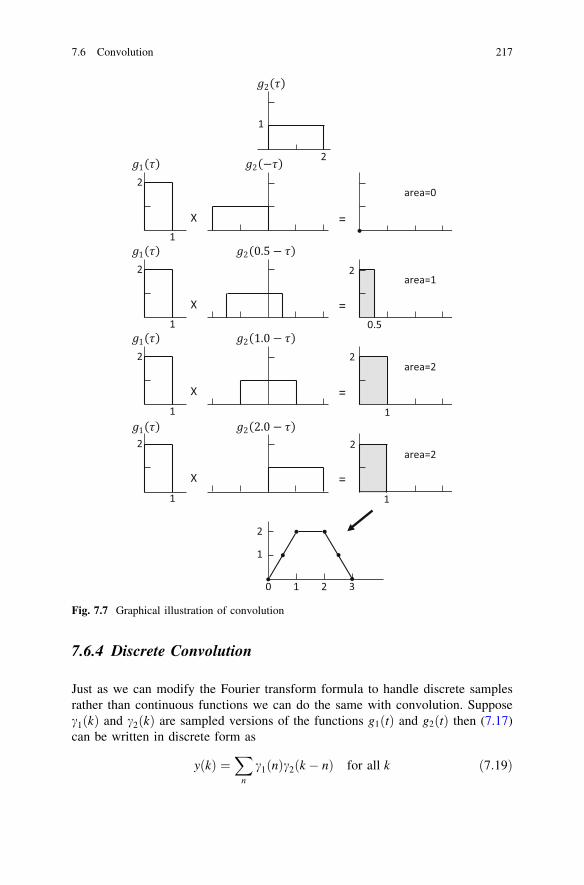
We can understand the convolution operation if we break it down into thefollowing four steps, which are illustrated in Fig. 7.7:

i. Folding: form g2ð�sÞ by taking the mirror image of g2ðsÞ about the vertical axisii. Shifting: form g2ðt � sÞ by shifting g2ð�sÞ by the variable amount tiii. Multiplication: form the product g1 sð Þg2 t � sð Þiv. Integration: compute the area under the product

7.6.2 Convolution with an Impulse

Convolution of a function with an impulse is important in understanding sampling.The delta function sifting theorem in (7.8) gives

y tð Þ ¼ g tð Þ��d t � t0ð Þ ¼Z

1

�1

g sð Þd t � s� t0ð Þds ¼ gðt � t0Þ

Thus, the result is to shift the function to a new origin. Clearly, fort0 ¼ 0; y tð Þ ¼ g tð Þ:

7.6.3 The Convolution Theorem

This theorem can be verified using the definitions of convolution and the Fouriertransform.8 It has two forms:

If y tð Þ ¼ g1 tð Þ��g2 tð Þ then Y xð Þ ¼ G1 xð ÞG2ðxÞ ð7:18aÞ

If Y xð Þ ¼ G1 xð Þ��G2ðxÞ then y tð Þ ¼ 2pg1 tð Þg2ðtÞ ð7:18bÞ

8 See A. Papoulis, Circuits and Systems: a Modern Approach, Holt-Saunders, Tokyo, 1980, andBrigham, loc. cit.


7.6.4 Discrete Convolution

Just as we can modify the Fourier transform formula to handle discrete samplesrather than continuous functions we can do the same with convolution. Supposec1 kð Þ and c2 kð Þ are sampled versions of the functions g1 tð Þ and g2 tð Þ then (7.17)can be written in discrete form as

y kð Þ ¼X

n

c1 nð Þc2 k � nð Þ for all k ð7:19Þ

Fig. 7.7 Graphical illustration of convolution

7.6 Convolution 217

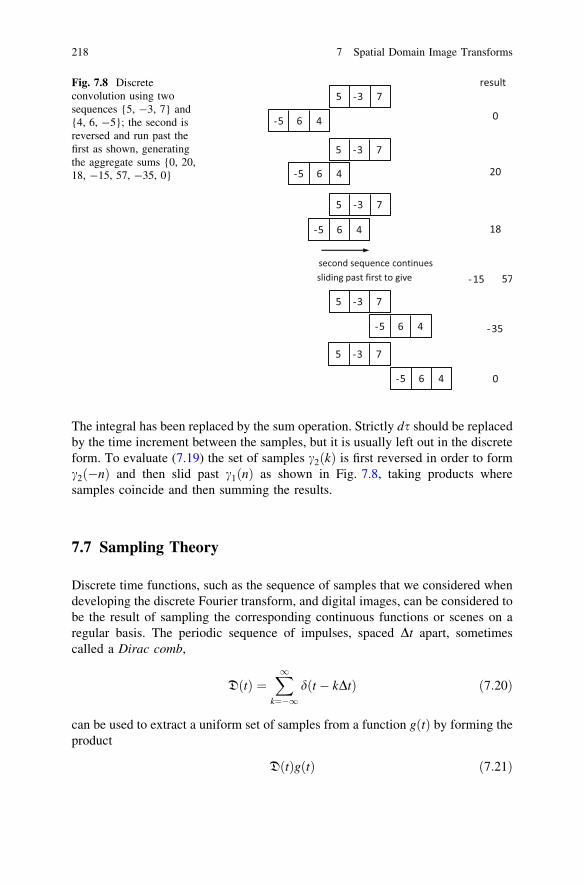
The integral has been replaced by the sum operation. Strictly ds should be replacedby the time increment between the samples, but it is usually left out in the discreteform. To evaluate (7.19) the set of samples c2 kð Þ is first reversed in order to formc2 �nð Þ and then slid past c1 nð Þ as shown in Fig. 7.8, taking products wheresamples coincide and then summing the results.

7.7 Sampling Theory

Discrete time functions, such as the sequence of samples that we considered whendeveloping the discrete Fourier transform, and digital images, can be considered tobe the result of sampling the corresponding continuous functions or scenes on aregular basis. The periodic sequence of impulses, spaced Dt apart, sometimescalled a Dirac comb,

D tð Þ ¼X

1

k¼�1dðt � kDtÞ ð7:20Þ

can be used to extract a uniform set of samples from a function g tð Þ by forming theproduct

D tð Þg tð Þ ð7:21Þ

Fig. 7.8 Discreteconvolution using twosequences {5, -3, 7} and{4, 6, -5}; the second isreversed and run past thefirst as shown, generatingthe aggregate sums {0, 20,18, -15, 57, -35, 0}


From (7.7) this is seen to be a sequence of samples of value g kTð Þd t � kDtð Þ; whichwe represent by c kð Þ. Despite the undefined magnitude of the delta function we willbe content in this treatment to regard the product simply as a sample of the functioncðtÞ, so that (7.21) can be interpreted as a set of uniformly spaced samples of cðtÞ.

It is important now to know the Fourier transform of the samples in (7.21). Wewill find that by calling on the convolution theorem in (7.18b), which requires theFourier transforms of g tð Þ and D tð Þ: Since D tð Þ is periodic we can work via theFourier series coefficient formula of (7.10b), which shows

Dn ¼1Dt

Z

Dt=2

�Dt=2

dðtÞe�jnx0tdt ¼ 1Dt

so that from (7.12) the Fourier transform of the periodic sequence of impulses in(7.20) is

D xð Þ ¼ 2pDt

X

1

n¼�1dðx� nxsÞ ð7:22Þ

in which xs ¼ 2p=Dt: Thus, the Fourier transform of the periodic sequence ofimpulses spaced Dt apart in the time domain is itself a periodic sequence ofimpulses in the frequency domain spaced apart 2p

Dt rad s�1; or 1Dt Hz:

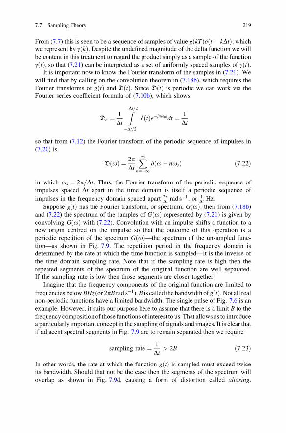
Suppose gðtÞ has the Fourier transform, or spectrum, GðxÞ; then from (7.18b)and (7.22) the spectrum of the samples of GðxÞ represented by (7.21) is given byconvolving GðxÞ with (7.22). Convolution with an impulse shifts a function to anew origin centred on the impulse so that the outcome of this operation is aperiodic repetition of the spectrum GðxÞ—the spectrum of the unsampled func-tion—as shown in Fig. 7.9. The repetition period in the frequency domain isdetermined by the rate at which the time function is sampled—it is the inverse ofthe time domain sampling rate. Note that if the sampling rate is high then therepeated segments of the spectrum of the original function are well separated.If the sampling rate is low then those segments are closer together.

Imagine that the frequency components of the original function are limited tofrequencies below BHz (or 2pB rad s�1). B is called the bandwidth of g tð Þ:Not all realnon-periodic functions have a limited bandwidth. The single pulse of Fig. 7.6 is anexample. However, it suits our purpose here to assume that there is a limit B to thefrequency composition of those functions of interest to us. That allows us to introducea particularly important concept in the sampling of signals and images. It is clear thatif adjacent spectral segments in Fig. 7.9 are to remain separated then we require

sampling rate ¼ 1Dt

[ 2B ð7:23Þ

In other words, the rate at which the function gðtÞ is sampled must exceed twiceits bandwidth. Should that not be the case then the segments of the spectrum willoverlap as shown in Fig. 7.9d, causing a form of distortion called aliasing.

7.7 Sampling Theory 219

The sampling rate of 2B in (7.23) is called the Nyquist rate. Equation (7.23) isoften called the sampling theorem.

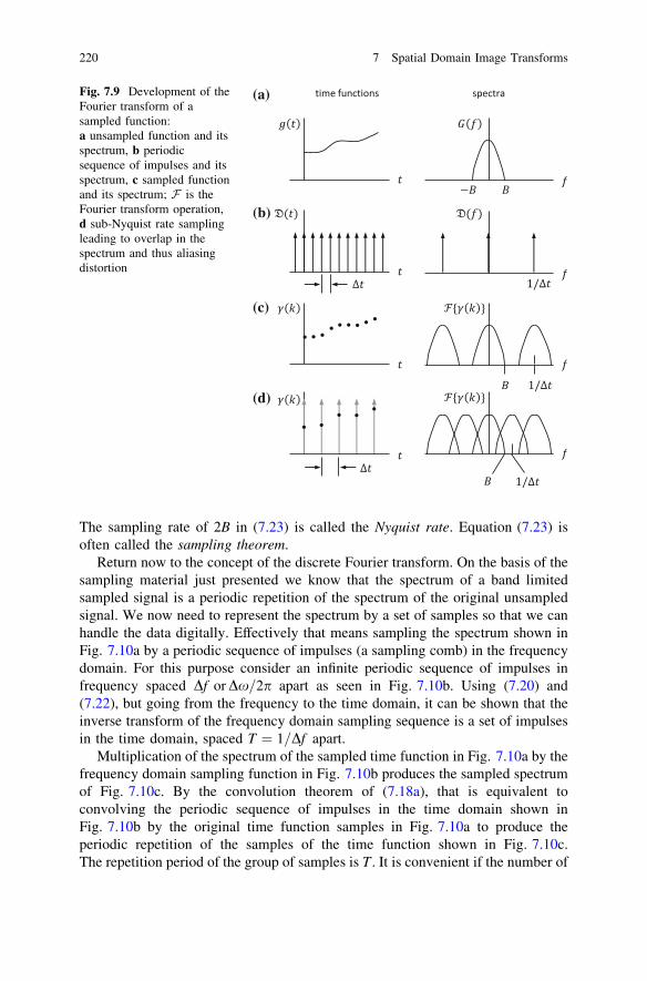
Return now to the concept of the discrete Fourier transform. On the basis of thesampling material just presented we know that the spectrum of a band limitedsampled signal is a periodic repetition of the spectrum of the original unsampledsignal. We now need to represent the spectrum by a set of samples so that we canhandle the data digitally. Effectively that means sampling the spectrum shown inFig. 7.10a by a periodic sequence of impulses (a sampling comb) in the frequencydomain. For this purpose consider an infinite periodic sequence of impulses infrequency spaced Df or Dx=2p apart as seen in Fig. 7.10b. Using (7.20) and(7.22), but going from the frequency to the time domain, it can be shown that theinverse transform of the frequency domain sampling sequence is a set of impulsesin the time domain, spaced T ¼ 1=Df apart.

Multiplication of the spectrum of the sampled time function in Fig. 7.10a by thefrequency domain sampling function in Fig. 7.10b produces the sampled spectrumof Fig. 7.10c. By the convolution theorem of (7.18a), that is equivalent toconvolving the periodic sequence of impulses in the time domain shown inFig. 7.10b by the original time function samples in Fig. 7.10a to produce theperiodic repetition of the samples of the time function shown in Fig. 7.10c.The repetition period of the group of samples is T . It is convenient if the number of

(a)

(b)

(c)

(d)

Fig. 7.9 Development of theFourier transform of asampled function:a unsampled function and itsspectrum, b periodicsequence of impulses and itsspectrum, c sampled functionand its spectrum; F is theFourier transform operation,d sub-Nyquist rate samplingleading to overlap in thespectrum and thus aliasingdistortion


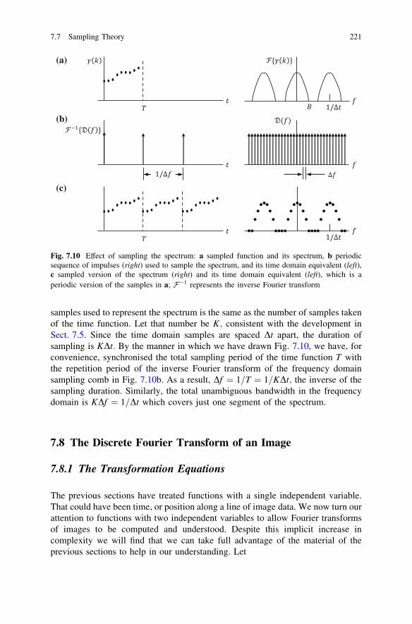
samples used to represent the spectrum is the same as the number of samples takenof the time function. Let that number be K; consistent with the development inSect. 7.5. Since the time domain samples are spaced Dt apart, the duration ofsampling is KDt: By the manner in which we have drawn Fig. 7.10, we have, forconvenience, synchronised the total sampling period of the time function T withthe repetition period of the inverse Fourier transform of the frequency domainsampling comb in Fig. 7.10b. As a result, Df ¼ 1=T ¼ 1=KDt; the inverse of thesampling duration. Similarly, the total unambiguous bandwidth in the frequencydomain is KDf ¼ 1=Dt which covers just one segment of the spectrum.

7.8 The Discrete Fourier Transform of an Image

7.8.1 The Transformation Equations

The previous sections have treated functions with a single independent variable.That could have been time, or position along a line of image data. We now turn ourattention to functions with two independent variables to allow Fourier transformsof images to be computed and understood. Despite this implicit increase incomplexity we will find that we can take full advantage of the material of theprevious sections to help in our understanding. Let

(a)

(b)

(c)

Fig. 7.10 Effect of sampling the spectrum: a sampled function and its spectrum, b periodicsequence of impulses (right) used to sample the spectrum, and its time domain equivalent (left),c sampled version of the spectrum (right) and its time domain equivalent (left), which is aperiodic version of the samples in a; F�1 represents the inverse Fourier transform

7.7 Sampling Theory 221

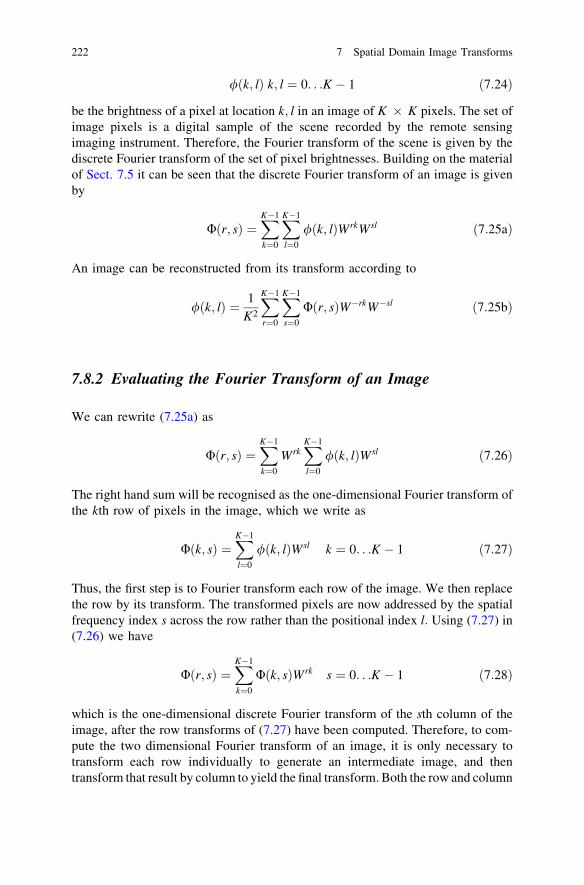
/ k; lð Þ k; l ¼ 0. . .K � 1 ð7:24Þ

be the brightness of a pixel at location k; l in an image of K � K pixels. The set ofimage pixels is a digital sample of the scene recorded by the remote sensingimaging instrument. Therefore, the Fourier transform of the scene is given by thediscrete Fourier transform of the set of pixel brightnesses. Building on the materialof Sect. 7.5 it can be seen that the discrete Fourier transform of an image is givenby

U r; sð Þ ¼X

K�1

k¼0

X

K�1

l¼0

/ k; lð ÞWrkWsl ð7:25aÞ

An image can be reconstructed from its transform according to

/ k; lð Þ ¼ 1K2

X

K�1

r¼0

X

K�1

s¼0

U r; sð ÞW�rkW�sl ð7:25bÞ

7.8.2 Evaluating the Fourier Transform of an Image

We can rewrite (7.25a) as

U r; sð Þ ¼X

K�1

k¼0

WrkX

K�1

l¼0

/ k; lð ÞWsl ð7:26Þ

The right hand sum will be recognised as the one-dimensional Fourier transform ofthe kth row of pixels in the image, which we write as

U k; sð Þ ¼X

K�1

l¼0

/ k; lð ÞWsl k ¼ 0. . .K � 1 ð7:27Þ

Thus, the first step is to Fourier transform each row of the image. We then replacethe row by its transform. The transformed pixels are now addressed by the spatialfrequency index s across the row rather than the positional index l: Using (7.27) in(7.26) we have

U r; sð Þ ¼X

K�1

k¼0

U k; sð ÞWrk s ¼ 0. . .K � 1 ð7:28Þ

which is the one-dimensional discrete Fourier transform of the sth column of theimage, after the row transforms of (7.27) have been computed. Therefore, to com-pute the two dimensional Fourier transform of an image, it is only necessary totransform each row individually to generate an intermediate image, and thentransform that result by column to yield the final transform. Both the row and column


transformations would be carried out using the fast Fourier transform algorithm,which requires K2log2K complex multiplications to transform the complete image.

7.8.3 The Concept of Spatial Frequency

Entries in the Fourier transformed image U r; sð Þ represent the composition of theoriginal image in terms of spatial frequency components, vertically and horizon-tally. Spatial frequency is the image analogue of the time frequency of signal.A sinusoidal function with a high frequency alternates rapidly, whereas alow-frequency function changes slowly with time. Similarly, an image with highspatial frequency in, say, the horizontal direction shows frequent changes ofbrightness with position horizontally. A picture of a crowd of people would be aparticular example, whereas a head and shoulders view of a person reading thenews on television is likely to be characterised mainly by a low spatial frequencies.Typically, an image is composed of a collection of both horizontal and verticalcomponents with different spatial frequencies of differing strengths. They are whatthe discrete Fourier transform describes.

The upper left-hand pixel in U r; sð Þ—U 0; 0ð Þ—is the average brightness valueof the image. In engineering this would sometimes be called the DC value. That isthe component of the spectrum with zero frequency variation in both directions.Thereafter, pixels in U r; sð Þ both horizontally and vertically represent componentswith frequencies that increment by 1=K where the original image is of size K � K:In most cases we would know the scale of the image, in other words the distanceon the ground covered by the K pixels across the lines and down the columns. Thatallows us to define the spatial frequency increment in terms of metres-1. Forexample, if an image covered 5 9 5 km, then the spatial frequency increment inboth directions is 2 9 10-4 m-1.

7.8.4 Displaying the DFT of an Image

In Fig. 7.9 we saw that the one dimensional discrete Fourier transformation of afunction is periodic with period K: The same is true of the discrete Fourier transformof an image. The K � K pixels of U r; sð Þ can be viewed as one period of aninfinitely periodic two-dimensional array in the manner depicted in Fig. 7.11.We also saw that the amplitude spectrum of the one dimensional DFT is symmetricabout K=2: Similarly U r; sð Þ is symmetric about its centre. Therefore, no newamplitude information is shown by displaying transform pixels horizontally andvertically beyond K=2: Rather than ignore them (since their accompanying phase isimportant) the display is adjusted as shown in Fig. 7.11 to bring U 0; 0ð Þ to thecentre. In that manner the pixel at the centre of the Fourier transform array repre-sents the image average brightness value. Pixels away from the centre represent the

7.8 The Discrete Fourier Transform of an Image 223

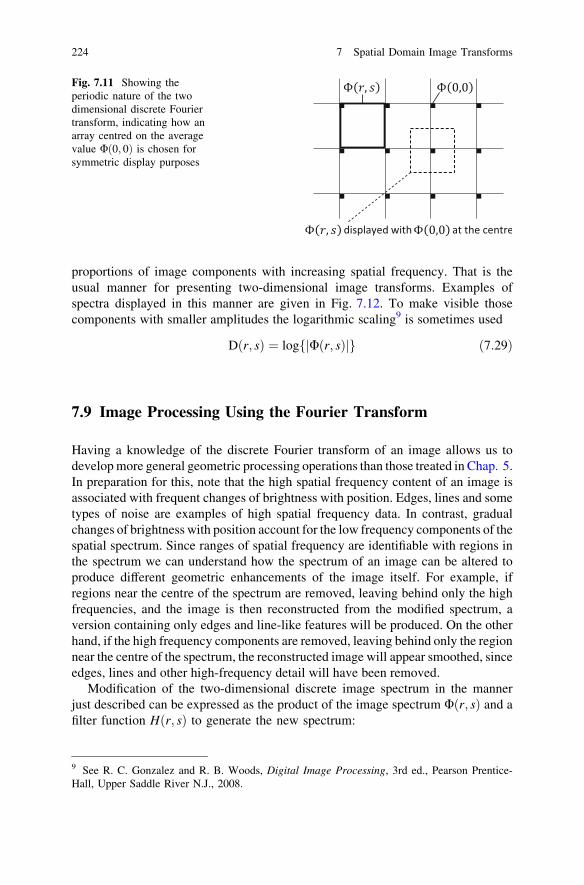
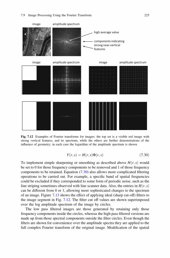
proportions of image components with increasing spatial frequency. That is theusual manner for presenting two-dimensional image transforms. Examples ofspectra displayed in this manner are given in Fig. 7.12. To make visible thosecomponents with smaller amplitudes the logarithmic scaling9 is sometimes used

D r; sð Þ ¼ logf U r; sð Þj jg ð7:29Þ

7.9 Image Processing Using the Fourier Transform

Having a knowledge of the discrete Fourier transform of an image allows us todevelop more general geometric processing operations than those treated in Chap. 5.In preparation for this, note that the high spatial frequency content of an image isassociated with frequent changes of brightness with position. Edges, lines and sometypes of noise are examples of high spatial frequency data. In contrast, gradualchanges of brightness with position account for the low frequency components of thespatial spectrum. Since ranges of spatial frequency are identifiable with regions inthe spectrum we can understand how the spectrum of an image can be altered toproduce different geometric enhancements of the image itself. For example, ifregions near the centre of the spectrum are removed, leaving behind only the highfrequencies, and the image is then reconstructed from the modified spectrum, aversion containing only edges and line-like features will be produced. On the otherhand, if the high frequency components are removed, leaving behind only the regionnear the centre of the spectrum, the reconstructed image will appear smoothed, sinceedges, lines and other high-frequency detail will have been removed.

Modification of the two-dimensional discrete image spectrum in the mannerjust described can be expressed as the product of the image spectrum U r; sð Þ and afilter function H r; sð Þ to generate the new spectrum:

Fig. 7.11 Showing theperiodic nature of the twodimensional discrete Fouriertransform, indicating how anarray centred on the averagevalue U 0; 0ð Þ is chosen forsymmetric display purposes

9 See R. C. Gonzalez and R. B. Woods, Digital Image Processing, 3rd ed., Pearson Prentice-Hall, Upper Saddle River N.J., 2008.


http://dx.doi.org/10.1007/978-3-642-30062-2_5

http://dx.doi.org/10.1007/978-3-642-30062-2_5

Y r; sð Þ ¼ Hðr; sÞU r; sð Þ ð7:30Þ

To implement simple sharpening or smoothing as described above Hðr; sÞ wouldbe set to 0 for those frequency components to be removed and 1 of those frequencycomponents to be retained. Equation (7.30) also allows more complicated filteringoperations to be carried out. For example, a specific band of spatial frequenciescould be excluded if they corresponded to some form of periodic noise, such as theline striping sometimes observed with line scanner data. Also, the entries in Hðr; sÞcan be different from 0 or 1, allowing more sophisticated changes to the spectrumof an image. Figure 7.13 shows the effect of applying ideal (sharp cut-off) filters tothe image segment in Fig. 7.12. The filter cut off values are shown superimposedover the log amplitude spectrum of the image by circles.

The low pass filtered images are those generated by retaining only thosefrequency components inside the circles, whereas the high pass filtered versions aremade up from those spectral components outside the filter circles. Even though thefilters are shown for convenience over the amplitude spectra they are applied to thefull complex Fourier transform of the original image. Modification of the spatial

Fig. 7.12 Examples of Fourier transforms for images: the top set is a visible red image withstrong vertical features, and its spectrum, while the others are further demonstrations of theinfluence of geometry; in each case the logarithm of the amplitude spectrum is shown

7.9 Image Processing Using the Fourier Transform 225

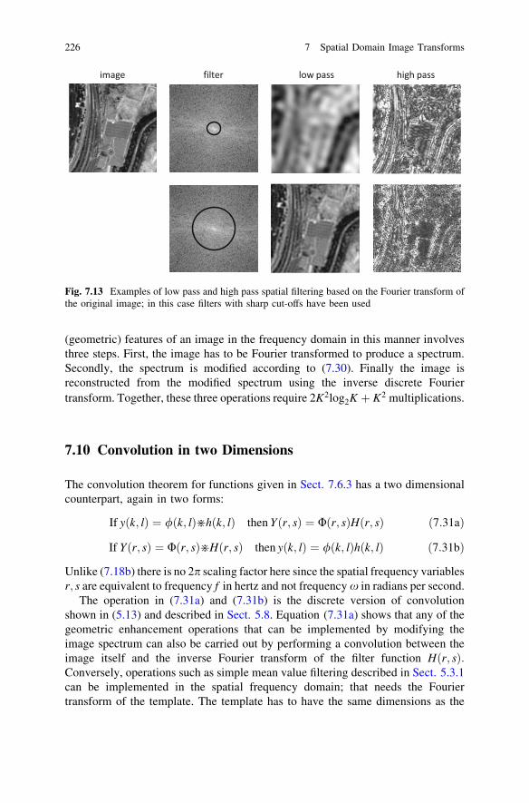
(geometric) features of an image in the frequency domain in this manner involvesthree steps. First, the image has to be Fourier transformed to produce a spectrum.Secondly, the spectrum is modified according to (7.30). Finally the image isreconstructed from the modified spectrum using the inverse discrete Fouriertransform. Together, these three operations require 2K2log2K þ K2 multiplications.

7.10 Convolution in two Dimensions

The convolution theorem for functions given in Sect. 7.6.3 has a two dimensionalcounterpart, again in two forms:

If y k; lð Þ ¼ / k; lð Þ��h k; lð Þ then Y r; sð Þ ¼ U r; sð ÞHðr; sÞ ð7:31aÞ

If Y r; sð Þ ¼ U r; sð Þ��Hðr; sÞ then y k; lð Þ ¼ / k; lð Þhðk; lÞ ð7:31bÞ

Unlike (7.18b) there is no 2p scaling factor here since the spatial frequency variablesr; s are equivalent to frequency f in hertz and not frequency x in radians per second.

The operation in (7.31a) and (7.31b) is the discrete version of convolutionshown in (5.13) and described in Sect. 5.8. Equation (7.31a) shows that any of thegeometric enhancement operations that can be implemented by modifying theimage spectrum can also be carried out by performing a convolution between theimage itself and the inverse Fourier transform of the filter function Hðr; sÞ:Conversely, operations such as simple mean value filtering described in Sect. 5.3.1can be implemented in the spatial frequency domain; that needs the Fouriertransform of the template. The template has to have the same dimensions as the

Fig. 7.13 Examples of low pass and high pass spatial filtering based on the Fourier transform ofthe original image; in this case filters with sharp cut-offs have been used


http://dx.doi.org/10.1007/978-3-642-30062-2_5

http://dx.doi.org/10.1007/978-3-642-30062-2_5

http://dx.doi.org/10.1007/978-3-642-30062-2_5

http://dx.doi.org/10.1007/978-3-642-30062-2_5

http://dx.doi.org/10.1007/978-3-642-30062-2_5

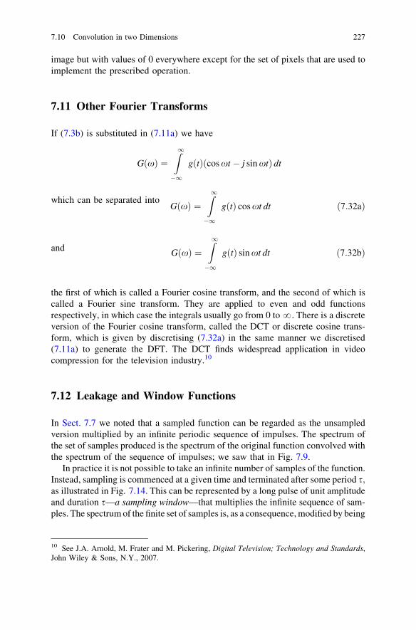
image but with values of 0 everywhere except for the set of pixels that are used toimplement the prescribed operation.

7.11 Other Fourier Transforms

If (7.3b) is substituted in (7.11a) we have

G xð Þ ¼Z

1

�1

g tð Þðcos xt � j sin xtÞ dt

which can be separated intoG xð Þ ¼

Z

1

�1

g tð Þ cos xt dt ð7:32aÞ

and G xð Þ ¼Z

1

�1

g tð Þ sin xt dt ð7:32bÞ

the first of which is called a Fourier cosine transform, and the second of which iscalled a Fourier sine transform. They are applied to even and odd functionsrespectively, in which case the integrals usually go from 0 to ?. There is a discreteversion of the Fourier cosine transform, called the DCT or discrete cosine trans-form, which is given by discretising (7.32a) in the same manner we discretised(7.11a) to generate the DFT. The DCT finds widespread application in videocompression for the television industry.10

7.12 Leakage and Window Functions

In Sect. 7.7 we noted that a sampled function can be regarded as the unsampledversion multiplied by an infinite periodic sequence of impulses. The spectrum ofthe set of samples produced is the spectrum of the original function convolved withthe spectrum of the sequence of impulses; we saw that in Fig. 7.9.

In practice it is not possible to take an infinite number of samples of the function.Instead, sampling is commenced at a given time and terminated after some period s;as illustrated in Fig. 7.14. This can be represented by a long pulse of unit amplitudeand duration s—a sampling window—that multiplies the infinite sequence of sam-ples. The spectrum of the finite set of samples is, as a consequence, modified by being

10 See J.A. Arnold, M. Frater and M. Pickering, Digital Television; Technology and Standards,John Wiley & Sons, N.Y., 2007.

7.10 Convolution in two Dimensions 227

convolved by the spectrum of the sampling window, again as illustrated in Fig. 7.14.Since the sampling window is a rectangular pulse its Fourier transform is as shown inFig. 7.6. Because the pulse is long compared with the sampling interval, thespectrum shown in Fig. 7.6 is compressed and looks like a finite amplitude impulse,thus approximating well the situation with an infinite sampling comb. Howeverwhen finite in length, its side lobes cause problems during convolution with thespectrum of the sequence of samples, causing distortion, as depicted in Fig. 7.14.

To minimise that form of distortion, which is referred to as leakage, the rect-angular sampling window is replaced by a function which avoids the sharp turn onand turn off with time that characterises the rectangular function. There are severalcandidates for these so-called window functions,11 perhaps the most common ofwhich is the raised cosine or Hanning window:

w tð Þ ¼ 0:5� 0:5 cos2pt

s

� �

ð7:33Þ

This has smaller side lobes in its spectrum than the simple rectangular pulse and,as a result, leads to less leakage distortion.

(a)

(b)

(c)

(d)

Fig. 7.14 Demonstrating theeffect of leakage distortion:a time signal and itsspectrum, b infinite sequenceof sampling impulses and itsspectrum, c finite timesampling window and itsspectrum, and d the result offinite time sampling as aproduct in the time domainand a convolution in thefrequency domain

11 An excellent treatment of leakage and the use of window functions is given in E.O Brigham,The Fast Fourier Transform and its Applications, Prentice-Hall, N.J., 1988.


If the function being sampled is periodic, and the samples are taken over one orseveral full periods, leakage will not occur. Otherwise it is always a matter forconsideration, and window functions generally need to be used.

7.13 The Wavelet Transform

7.13.1 Background

In principle, the Fourier transform can be used to represent any signal by a col-lection, sometimes infinite, of sinusoidal functions. Likewise, the two-dimensionalspatial Fourier transform can be used to model the distribution of brightness valuesin an image by using a collection of two dimensional sinusoidal basis functions.

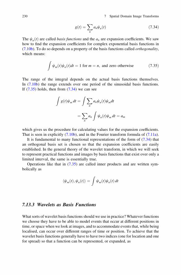
Many of the image features of interest to us occur over a short distance,including edges and lines. Also, when dealing with functions of time, we aresometimes interested in representing short time signals rather than those that lastfor a long period. As an illustration, an organ playing a single, pure tone generatesa signal that is well-modelled by simple sinusoids. In contrast, when a single noteis played on a piano we have an approximately sinusoidal signal, at the frequencyof the key played, which lasts for just a short time. We can still find the Fouriertransform representation of the piano note—its spectrum—but there are other waysto represent such a short time signals, just as there are other ways of representingor modelling image features that change over a short distance. The wavelettransformation is generally more useful in such situations than the Fourier trans-form. It is based on the definition of a wavelet, which is a wavelike signal that islimited in time (or space, in the spatial domain). The theory of the wavelettransformation is quite detailed, especially when treated comprehensively.12 Herewe provide a simple introduction in which the mathematical detail is kept to aminimum and some concepts are simplified, so that its common usage in imageprocessing can be understood. It finds most application in image compression andcoding, and in the detection of localised features such as edges and lines.

7.13.2 Orthogonal Functions and Inner Products

The Fourier series and transform expansions of (7.10a) and (7.11b) are specialcases of the more general representation of a function by a sum of other functions,expressible as

12 For a detailed treatment of wavelets see G. Strang and T. Nguyen, Wavelets and Filter Banks,Wellesley-Cambridge, Mass., 1996, and K.R. Castleman, Digital Image Processing, 2nd ed.,Prentice Hall, N.J., 1996.

7.12 Leakage and Window Functions 229

g tð Þ ¼X

n

anwnðtÞ ð7:34Þ

The wnðtÞ are called basis functions and the an are expansion coefficients. We sawhow to find the expansion coefficients for complex exponential basis functions in(7.10b). To do so depends on a property of the basis functions called orthogonality,which means:

Z

wm tð Þwn tð Þdt ¼ 1 for m ¼ n; and zero otherwise ð7:35Þ

The range of the integral depends on the actual basis functions themselves.In (7.10b) the range extends over one period of the sinusoidal basis functions.If (7.35) holds, then from (7.34) we can see

Z

g tð Þwm dt ¼Z

X

n

anwnðtÞwmdt

¼X

n

an

Z

wnðtÞwm dt ¼ am

which gives us the procedure for calculating values for the expansion coefficients.That is seen in explicitly (7.10b), and in the Fourier transform formula of (7.11a).

It is fundamental to many functional representations of the form of (7.34) thatan orthogonal basis set is chosen so that the expansion coefficients are easilyestablished. In the general theory of the wavelet transform, in which we will seekto represent practical functions and images by basis functions that exist over only alimited interval, the same is essentially true.

Operations like that in (7.35) are called inner products and are written sym-bolically as

hwm tð Þ;wn tð Þi ¼Z

wm tð Þwn tð Þ dt

7.13.3 Wavelets as Basis Functions

What sorts of wavelet basis functions should we use in practice? Whatever functionswe choose they have to be able to model events that occur at different positions intime, or space when we look at images, and to accommodate events that, while beinglocalised, can occur over different ranges of time or position. To achieve that thewavelet basis functions generally have to have two indices (one for location and onefor spread) so that a function can be represented, or expanded, as


g tð Þ ¼X

j;k

cj;kwj;k tð Þ ð7:36Þ

Figure 7.15 shows such a set of functions. We see that a fundamental function istranslated and scaled so that it can cover instances at different times and overdifferent durations.

Rather than define translations and scalings arbitrarily we restrict attention tobinary scalings, in which the range is shrunk by progressive factors of two, and todyadic translations, in which the shift amount is an integral multiple of the binaryscaling factor. That means that the set of wavelet functions we are dealing with arebuilt up from a basis function wðtÞ; sometimes called the mother wavelet orgenerating wavelet, such that all other wavelets are defined by

wj;k tð Þ ¼ 2j=2wð2 jt � kÞ ð7:37Þ

in which j is the scaling factor and k is the integral multiple of the scaling by whichthe shift occurs. The factor 2j=2 is included so that the integral of the squaredamplitude of the wavelet is unity, one of the requirements of a wavelet basisfunction. The relationship in (7.37) is applied in Fig. 7.15, although the amplitudescaling is omitted for clarity. Note that, apart from being integers, j and k arearbitrary at this stage. Putting (7.37) in (7.36) we have

Fig. 7.15 Some members ofa family of wavelets(Mexican hat) created by timescaling and translating a basicform (without any amplitudescaling)

7.13 The Wavelet Transform 231

g tð Þ ¼X

j;k

cj;k2j=2wð2 jt � kÞ ð7:38Þ

The set of coefficients cj;k is sometimes called the wavelet transform of gðtÞ; or itswavelet spectrum.

7.13.4 Dyadic Wavelets with Compact Support

It is possible to restrict further the set of wavelets of interest by establishing arelationship between j and k: If we constrain our attention to so-called compactfunctions gðtÞ that are zero outside the interval [0,1] we can use a single index n todescribe the set of basis functions, where

n ¼ 2 j þ k

The basis functions, while still having the general form in (7.37), can then beindexed by the single integer n; in which case the wavelet expansion, or repre-sentation, of the time restricted signal is

gðtÞ ¼X

1

n¼0

cnwnðtÞ ð7:39Þ

The expansion coefficients are given by

cn ¼Z

1

�1

gðtÞwnðtÞ dt ð7:40Þ

We do not pursue this version explicitly any further here.

7.13.5 Choosing the Wavelets

Not all finite time (or space) functions can be used as wavelets; it is only those thatsatisfy the so-called admissibility criterion that can be employed in waveletexpansions.13 Fortunately, for most of the work of interest to remote sensing imageprocessing a simpler approach is possible, based on the concept of filter banks,which avoids the need specifically to treat a range of candidate wavelet families.Although originally developed separately, the filter bank and wavelet approachesare related. Rather than continue with the theoretical development of continuouswavelets as such, we will now focus on filter banks. As the name suggests a filter

13 See Castleman, loc. cit., Sect. 14.2.1, and Problem 7.14.


bank is made up of a set of filters that respond to different frequency ranges in asignal or image. Each of the filters is a finite impulse response (FIR) digital filter.A background in that material, while helpful, is not required for the followingdevelopment.

7.13.6 Filter Banks

7.13.6.1 Sub Band Filtering, and Downsampling

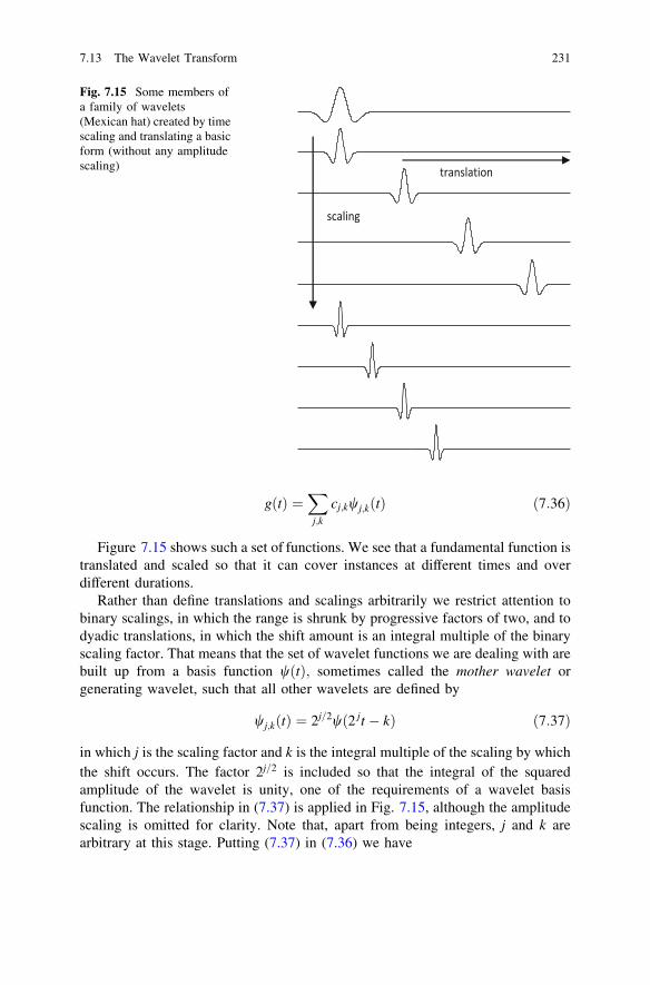
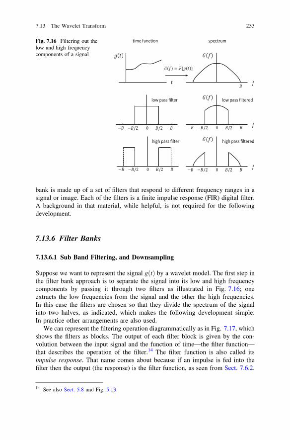
Suppose we want to represent the signal gðtÞ by a wavelet model. The first step inthe filter bank approach is to separate the signal into its low and high frequencycomponents by passing it through two filters as illustrated in Fig. 7.16; oneextracts the low frequencies from the signal and the other the high frequencies.In this case the filters are chosen so that they divide the spectrum of the signalinto two halves, as indicated, which makes the following development simple.In practice other arrangements are also used.

We can represent the filtering operation diagrammatically as in Fig. 7.17, whichshows the filters as blocks. The output of each filter block is given by the con-volution between the input signal and the function of time—the filter function—that describes the operation of the filter.14 The filter function is also called itsimpulse response. That name comes about because if an impulse is fed into thefilter then the output (the response) is the filter function, as seen from Sect. 7.6.2.

Fig. 7.16 Filtering out thelow and high frequencycomponents of a signal

14 See also Sect. 5.8 and Fig. 5.13.


http://dx.doi.org/10.1007/978-3-642-30062-2_5

http://dx.doi.org/10.1007/978-3-642-30062-2_5

http://dx.doi.org/10.1007/978-3-642-30062-2_5

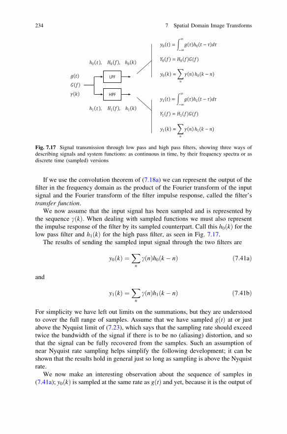
If we use the convolution theorem of (7.18a) we can represent the output of thefilter in the frequency domain as the product of the Fourier transform of the inputsignal and the Fourier transform of the filter impulse response, called the filter’stransfer function.

We now assume that the input signal has been sampled and is represented bythe sequence c kð Þ: When dealing with sampled functions we must also representthe impulse response of the filter by its sampled counterpart. Call this h0 kð Þ for thelow pass filter and h1 kð Þ for the high pass filter, as seen in Fig. 7.17.

The results of sending the sampled input signal through the two filters are

y0 kð Þ ¼X

n

c nð Þh0ðk � nÞ ð7:41aÞ

and

y1 kð Þ ¼X

n

c nð Þh1ðk � nÞ ð7:41bÞ

For simplicity we have left out limits on the summations, but they are understoodto cover the full range of samples. Assume that we have sampled gðtÞ at or justabove the Nyquist limit of (7.23), which says that the sampling rate should exceedtwice the bandwidth of the signal if there is to be no (aliasing) distortion, and sothat the signal can be fully recovered from the samples. Such an assumption ofnear Nyquist rate sampling helps simplify the following development; it can beshown that the results hold in general just so long as sampling is above the Nyquistrate.

We now make an interesting observation about the sequence of samples in(7.41a); y0 kð Þ is sampled at the same rate as gðtÞ and yet, because it is the output of

Fig. 7.17 Signal transmission through low pass and high pass filters, showing three ways ofdescribing signals and system functions: as continuous in time, by their frequency spectra or asdiscrete time (sampled) versions


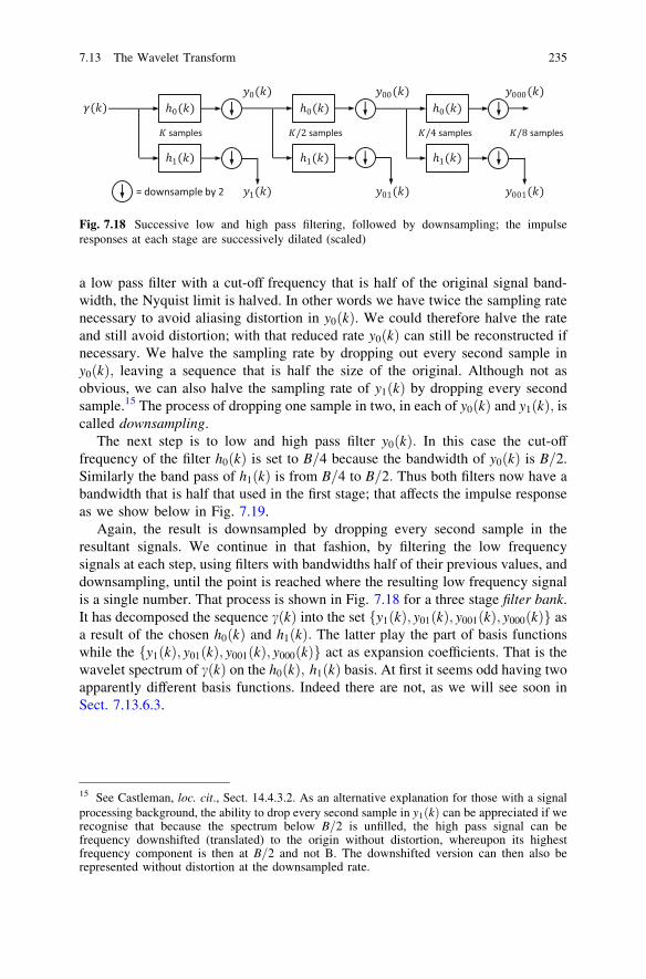
a low pass filter with a cut-off frequency that is half of the original signal band-width, the Nyquist limit is halved. In other words we have twice the sampling ratenecessary to avoid aliasing distortion in y0 kð Þ. We could therefore halve the rateand still avoid distortion; with that reduced rate y0 kð Þ can still be reconstructed ifnecessary. We halve the sampling rate by dropping out every second sample iny0 kð Þ; leaving a sequence that is half the size of the original. Although not asobvious, we can also halve the sampling rate of y1 kð Þ by dropping every secondsample.15 The process of dropping one sample in two, in each of y0 kð Þ and y1 kð Þ; iscalled downsampling.

The next step is to low and high pass filter y0 kð Þ: In this case the cut-offfrequency of the filter h0 kð Þ is set to B=4 because the bandwidth of y0 kð Þ is B=2.Similarly the band pass of h1 kð Þ is from B=4 to B=2: Thus both filters now have abandwidth that is half that used in the first stage; that affects the impulse responseas we show below in Fig. 7.19.

Again, the result is downsampled by dropping every second sample in theresultant signals. We continue in that fashion, by filtering the low frequencysignals at each step, using filters with bandwidths half of their previous values, anddownsampling, until the point is reached where the resulting low frequency signalis a single number. That process is shown in Fig. 7.18 for a three stage filter bank.It has decomposed the sequence c kð Þ into the set fy1 kð Þ; y01 kð Þ; y001 kð Þ; y000 kð Þg asa result of the chosen h0 kð Þ and h1 kð Þ: The latter play the part of basis functionswhile the fy1 kð Þ; y01 kð Þ; y001 kð Þ; y000 kð Þg act as expansion coefficients. That is thewavelet spectrum of c kð Þ on the h0 kð Þ; h1 kð Þ basis. At first it seems odd having twoapparently different basis functions. Indeed there are not, as we will see soon inSect. 7.13.6.3.

Fig. 7.18 Successive low and high pass filtering, followed by downsampling; the impulseresponses at each stage are successively dilated (scaled)

15 See Castleman, loc. cit., Sect. 14.4.3.2. As an alternative explanation for those with a signalprocessing background, the ability to drop every second sample in y1 kð Þ can be appreciated if werecognise that because the spectrum below B=2 is unfilled, the high pass signal can befrequency downshifted (translated) to the origin without distortion, whereupon its highestfrequency component is then at B=2 and not B. The downshifted version can then also berepresented without distortion at the downsampled rate.


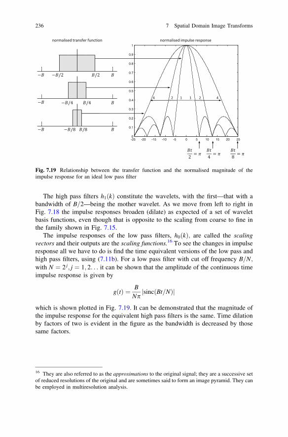
The high pass filters h1 kð Þ constitute the wavelets, with the first—that with abandwidth of B=2—being the mother wavelet. As we move from left to right inFig. 7.18 the impulse responses broaden (dilate) as expected of a set of waveletbasis functions, even though that is opposite to the scaling from coarse to fine inthe family shown in Fig. 7.15.

The impulse responses of the low pass filters, h0 kð Þ; are called the scalingvectors and their outputs are the scaling functions.16 To see the changes in impulseresponse all we have to do is find the time equivalent versions of the low pass andhigh pass filters, using (7.11b). For a low pass filter with cut off frequency B=N;with N ¼ 2 j; j ¼ 1; 2. . . it can be shown that the amplitude of the continuous timeimpulse response is given by

gðtÞ ¼ B

NpsincðBt=NÞj j

which is shown plotted in Fig. 7.19. It can be demonstrated that the magnitude ofthe impulse response for the equivalent high pass filters is the same. Time dilationby factors of two is evident in the figure as the bandwidth is decreased by thosesame factors.

Fig. 7.19 Relationship between the transfer function and the normalised magnitude of theimpulse response for an ideal low pass filter

16 They are also referred to as the approximations to the original signal; they are a successive setof reduced resolutions of the original and are sometimes said to form an image pyramid. They canbe employed in multiresolution analysis.


7.13.6.2 Reconstruction from the Wavelets, and Upsampling

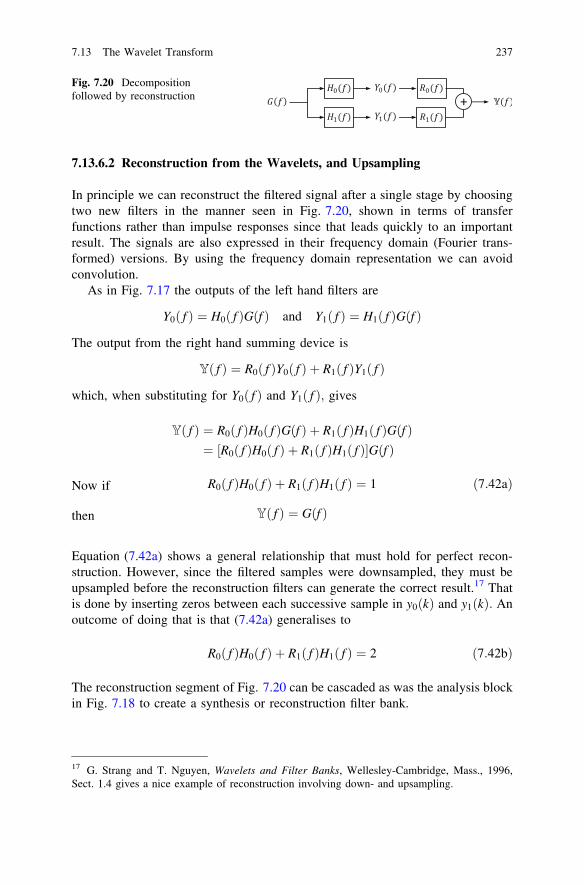
In principle we can reconstruct the filtered signal after a single stage by choosingtwo new filters in the manner seen in Fig. 7.20, shown in terms of transferfunctions rather than impulse responses since that leads quickly to an importantresult. The signals are also expressed in their frequency domain (Fourier trans-formed) versions. By using the frequency domain representation we can avoidconvolution.

As in Fig. 7.17 the outputs of the left hand filters are

Y0 fð Þ ¼ H0 fð ÞGðf Þ and Y1 fð Þ ¼ H1 fð ÞGðf Þ

The output from the right hand summing device is

Y fð Þ ¼ R0 fð ÞY0 fð Þ þ R1 fð ÞY1 fð Þ

which, when substituting for Y0 fð Þ and Y1 fð Þ; gives

Y fð Þ ¼ R0 fð ÞH0 fð ÞGðf Þ þ R1 fð ÞH1 fð ÞGðf Þ¼ ½R0 fð ÞH0 fð Þ þ R1 fð ÞH1 fð ÞGðf Þ

Now if R0 fð ÞH0 fð Þ þ R1 fð ÞH1 fð Þ ¼ 1 ð7:42aÞ

then Y fð Þ ¼ Gðf Þ

Equation (7.42a) shows a general relationship that must hold for perfect recon-struction. However, since the filtered samples were downsampled, they must beupsampled before the reconstruction filters can generate the correct result.17 Thatis done by inserting zeros between each successive sample in y0ðkÞ and y1ðkÞ: Anoutcome of doing that is that (7.42a) generalises to

R0 fð ÞH0 fð Þ þ R1 fð ÞH1 fð Þ ¼ 2 ð7:42bÞ

The reconstruction segment of Fig. 7.20 can be cascaded as was the analysis blockin Fig. 7.18 to create a synthesis or reconstruction filter bank.

Fig. 7.20 Decompositionfollowed by reconstruction

17 G. Strang and T. Nguyen, Wavelets and Filter Banks, Wellesley-Cambridge, Mass., 1996,Sect. 1.4 gives a nice example of reconstruction involving down- and upsampling.


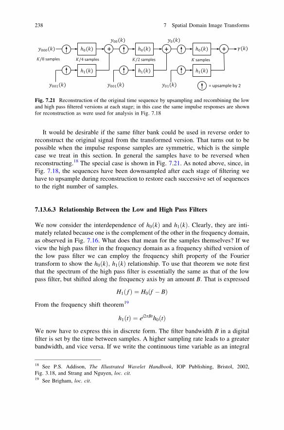
It would be desirable if the same filter bank could be used in reverse order toreconstruct the original signal from the transformed version. That turns out to bepossible when the impulse response samples are symmetric, which is the simplecase we treat in this section. In general the samples have to be reversed whenreconstructing.18 The special case is shown in Fig. 7.21. As noted above, since, inFig. 7.18, the sequences have been downsampled after each stage of filtering wehave to upsample during reconstruction to restore each successive set of sequencesto the right number of samples.

7.13.6.3 Relationship Between the Low and High Pass Filters

We now consider the interdependence of h0 kð Þ and h1 kð Þ: Clearly, they are inti-mately related because one is the complement of the other in the frequency domain,as observed in Fig. 7.16. What does that mean for the samples themselves? If weview the high pass filter in the frequency domain as a frequency shifted version ofthe low pass filter we can employ the frequency shift property of the Fouriertransform to show the h0 kð Þ; h1 kð Þ relationship. To use that theorem we note firstthat the spectrum of the high pass filter is essentially the same as that of the lowpass filter, but shifted along the frequency axis by an amount B: That is expressed

H1 fð Þ ¼ H0ðf � BÞ

From the frequency shift theorem19

h1 tð Þ ¼ ej2pBth0ðtÞ

We now have to express this in discrete form. The filter bandwidth B in a digitalfilter is set by the time between samples. A higher sampling rate leads to a greaterbandwidth, and vice versa. If we write the continuous time variable as an integral

Fig. 7.21 Reconstruction of the original time sequence by upsampling and recombining the lowand high pass filtered versions at each stage; in this case the same impulse responses are shownfor reconstruction as were used for analysis in Fig. 7.18

18 See P.S. Addison, The Illustrated Wavelet Handbook, IOP Publishing, Bristol, 2002,Fig. 3.18, and Strang and Nguyen, loc. cit.19 See Brigham, loc. cit.


multiple of the sampling interval t ¼ kDt then B ¼ 1=2Dt so that, in discrete form,the last expression becomes

h1 kð Þ ¼ ejpkh0ðkÞ

The complex exponential with an exponent that is an integral multiple of p is �1:That tells us that the impulse response of the high pass filter is the same as that ofthe low pass filter, except that every odd numbered sample has its sign reversed.That applies for the case of the ideal low and high pass filters. More generally,it also requires a reversal of the order of the samples.20

7.13.7 Choice of Wavelets

In the filter bank development of Sect. 7.13.6 we have presented a decompositionand synthesis methodology that emulates wavelet analysis. It is based on thespecification of the impulse responses of the low and high pass filters, which wenow need to be more specific about because they describe the wavelets that are thebasis functions for a given situation.

Although (7.38) is acceptable as a general expression of a wavelet expansion, itis more convenient, when comparing it to the filter bank approach, if we re-expressthe decomposition as the combination of an expansion in wavelets wðtÞ plus acompanion scaling function uðtÞ in the form

g tð Þ ¼ Au tð Þ þX

j;k

cj;k2j=2wð2 jt � kÞ ð7:43Þ

The scaling function satisfies the scaling or dilation equation

u tð Þ ¼X

k

h0ðkÞu 2t � kð Þ ð7:44Þ

while the mother wavelet satisfies the wavelet equation

w tð Þ ¼X

k

h1ðkÞu 2t � kð Þ ð7:45Þ

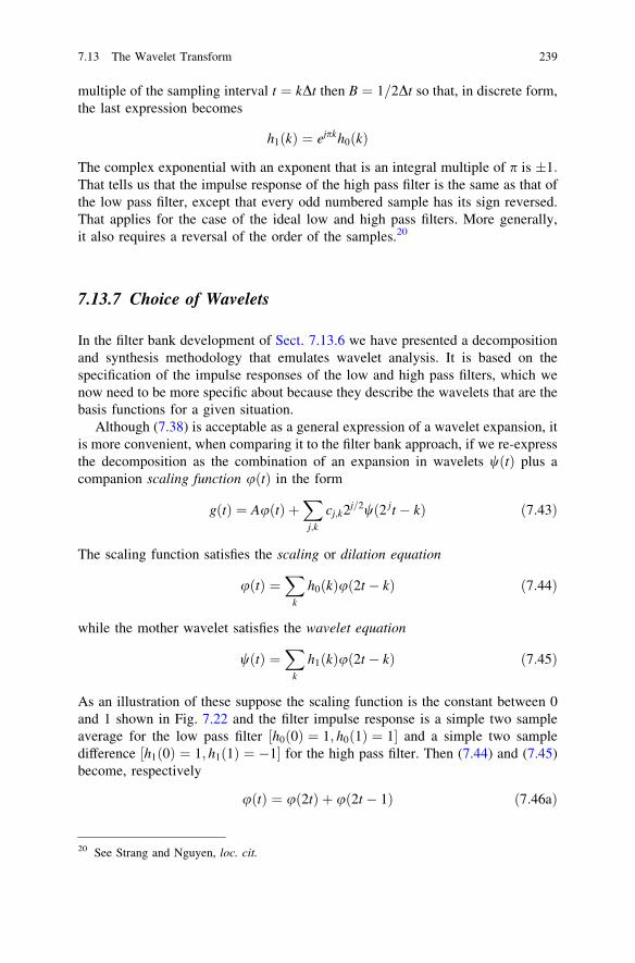
As an illustration of these suppose the scaling function is the constant between 0and 1 shown in Fig. 7.22 and the filter impulse response is a simple two sampleaverage for the low pass filter ½h0 0ð Þ ¼ 1; h0 1ð Þ ¼ 1 and a simple two sampledifference ½h1 0ð Þ ¼ 1; h1 1ð Þ ¼ �1 for the high pass filter. Then (7.44) and (7.45)become, respectively

u tð Þ ¼ u 2tð Þ þ u 2t � 1ð Þ ð7:46aÞ

20 See Strang and Nguyen, loc. cit.


w tð Þ ¼ u 2tð Þ � u 2t � 1ð Þ ð7:46bÞ

which are also shown plotted in Fig. 7.22. The recurrence relationship in (7.37)then allows others in the set to be generated. These are the Haar wavelets. Whenused as the basis for a filter bank implementation of the wavelet transform theexpressions in (7.46a) and (7.46b) need to be scaled by 1=

ffiffiffi

2p

to give the correctsquare integral for the wavelets.

Haar wavelets are generated by the simple sum and difference filters above.A variety of other types is available, many of which are examples of theDaubechies wavelets21 that can also be implemented readily as filter banks.The family of Daubechies wavelets includes the Haar wavelet as its simplest case.

Fig. 7.22 The Haar scalingfunction and waveletsgenerated with the scaling,dilation and recurrencerelations—this is the firstsubset of 8 Haar wavelets;also shown at the top is thescaling function on a halftime scale; note that the 2j=2

amplitude scaling in (7.37)has not been included

21 See Strang and Nguyen, loc. cit., and Addison, loc. cit., Fig. 3.15.


http://dx.doi.org/10.1007/978-3-642-30062-2_3

7.14 The Wavelet Transform of an Image

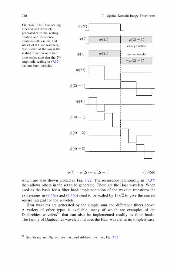
The application of the discrete wavelet transformation to imagery is similar to themanner in which the discrete Fourier transform is applied. First, the rows of theimage are transformed using the first stage process in Fig. 7.18. Every secondcolumn is then discarded, which corresponds to downsampling the row trans-formed data. Next the columns are transformed and every second row discarded.

As illustrated in Fig. 7.23 that leads to four new images:

• a version that has been low pass filtered in both row and column, and which isreferred to as the approximation image;

• a version that has been high pass filtered in the horizontal direction, therebyemphasising the horizontal edge information;

• a version that has been high pass filtered in the vertical direction, therebyemphasising the vertical edge information;

• a version that has been high pass filtered in both the vertical and horizontaldirections, thereby emphasising diagonal edge information.

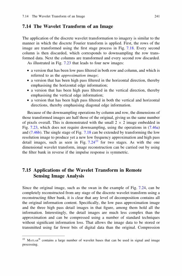
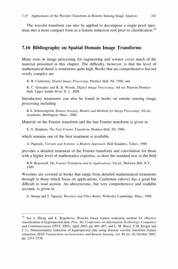
Because of the downsampling operations by column and row, the dimensions ofthose transformed images are half those of the original, giving us the same numberof pixels overall. This is demonstrated with the small 2 9 2 image embedded inFig. 7.23, which does not require downsampling, using the operations in (7.46a)and (7.46b). The single stage of Fig. 7.18 can be extended by transforming the lowresolution image to produce yet a new low frequency approximation and high passdetail images, such as seen in Fig. 7.2422 for two stages. As with the onedimensional wavelet transform, image reconstruction can be carried out by usingthe filter bank in reverse if the impulse response is symmetric.

7.15 Applications of the Wavelet Transform in RemoteSensing Image Analysis

Since the original image, such as the swan in the example of Fig. 7.24, can becompletely reconstructed from any stage of the discrete wavelet transform using areconstructing filter bank, it is clear that any level of decomposition contains allthe original information content. Specifically, the low pass approximation imageand the three high pass detail images in that figure, among them hold all theinformation. Interestingly, the detail images are much less complex than theapproximation and can be compressed using a number of standard techniqueswithout significant information loss. That allows the image data to be stored ortransmitted using far fewer bits of digital data than the original. Compression

22 MATLAB� contains a large number of wavelet bases that can be used in signal and image

processing.

7.14 The Wavelet Transform of an Image 241

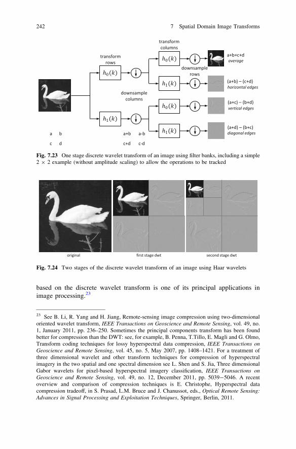
based on the discrete wavelet transform is one of its principal applications inimage processing.23

Fig. 7.23 One stage discrete wavelet transform of an image using filter banks, including a simple2 9 2 example (without amplitude scaling) to allow the operations to be tracked

Fig. 7.24 Two stages of the discrete wavelet transform of an image using Haar wavelets

23 See B. Li, R. Yang and H. Jiang, Remote-sensing image compression using two-dimensionaloriented wavelet transform, IEEE Transactions on Geoscience and Remote Sensing, vol. 49, no.1, January 2011, pp. 236–250. Sometimes the principal components transform has been foundbetter for compression than the DWT: see, for example, B. Penna, T.Tillo, E. Magli and G. Olmo,Transform coding techniques for lossy hyperspectral data compression, IEEE Transactions onGeoscience and Remote Sensing, vol. 45, no. 5, May 2007, pp. 1408–1421. For a treatment ofthree dimensional wavelet and other transform techniques for compression of hyperspectralimagery in the two spatial and one spectral dimension see L. Shen and S. Jia, Three dimensionalGabor wavelets for pixel-based hyperspectral imagery classification, IEEE Transactions onGeoscience and Remote Sensing, vol. 49, no. 12, December 2011, pp. 5039-5046. A recentoverview and comparison of compression techniques is E. Christophe, Hyperspectral datacompression tradeoff, in S. Prasad, L.M. Bruce and J. Chanussot, eds., Optical Remote Sensing:Advances in Signal Processing and Exploitation Techniques, Springer, Berlin, 2011.


The wavelet transform can also be applied to decompose a single pixel spec-trum into a more compact form as a feature reduction tool prior to classification.24

7.16 Bibliography on Spatial Domain Image Transforms

Many texts in image processing for engineering and science cover much of thematerial presented in this chapter. The difficulty, however, is that the level ofmathematical detail is sometimes quite high. Books that are comprehensive but notoverly complex are

K. R. Castleman, Digital Image Processing, Prentice Hall, NJ, 1996, and

R. C. Gonzalez and R. B. Woods, Digital Image Processing, 3rd ed. Pearson Prentice-Hall, Upper Saddle River N. J., 2008.

Introductory treatments can also be found in books on remote sensing imageprocessing including

R.A. Schowengerdt, Remote Sensing: Models and Methods for Image Processing, 3rd ed.,Academic, Burlington, Mass., 2006.

Material on the Fourier transform and the fast Fourier transform is given in

E. O. Brigham, The Fast Fourier Transform, Prentice-Hall, NJ, 1988,

which remains one of the best treatment is available.

A. Papoulis, Circuits and Systems: a Modern Approach, Holt-Saunders, Tokyo, 1980

provides a detailed treatment of the Fourier transform and convolution for thosewith a higher level of mathematics expertise, as does the standard text in the field

R.N. Bracewell, The Fourier Transform and its Applications, 3rd ed., McGraw-Hill, N.Y.,1999.

Wavelets are covered in books that range from detailed mathematical treatmentsthrough to those which focus on applications. Castleman (above) has a good butdifficult to read section. An idiosyncratic, but very comprehensive and readableaccount, is given in

G. Strang and T. Nguyen, Wavelets and Filter Banks, Wellesley-Cambridge, Mass., 1996

24 See J. Zheng and E. Regentova, Wavelet based feature reduction method for effectiveclassification of hyperspectral data, Proc. Int. Conference on Information Technology, Computersand Communications (ITCC 2003), April 2003, pp. 483–487, and L. M. Bruce, C.H. Kroger andJ. Li, Dimensionality reduction of hyperspectral data using discrete wavelet transform featureextraction, IEEE Transactions on Geoscience and Remote Sensing, vol. 40, no. 10, October 2002,pp. 2331–2338.

7.15 Applications of the Wavelet Transform in Remote Sensing Image Analysis 243

A good overview of the application of wavelets in a wide range of physicalsituations including medicine, finance, fluid flow, geophysics and mechanicalengineering will be found in

P.S. Addison, The Illustrated Wavelet Handbook, IOP Publishing, Bristol, 2002

while a very good discussion on wavelet applications in astronomical imageprocessing is given in

R. Berry and J. Burnell, The Handbook of Astronomical Image Processing, Willman-Bell,Richmond, VA, 2006.

This book also includes a helpful section on the use of the Fourier transform forimage filtering. It shows the use of wavelets for multiresolution image analysis andhow, by filtering specific wavelet components, features at particular levels of detailcan be enhanced. Other texts that could be consulted are

C. Sidney Burrus, R. A. Gopinath and H. Guo, Introduction to Wavelets and WaveletTransforms, Prentice Hall, Upper Saddle River, NJ, 1998, and

A.K. Chan and C. Peng, Wavelets for Sensing Technologies, Artech House, Norwood,MA, 2003

the last of which has a focus on SAR imagery and medical imaging.

7.17 Problems

7.1. Using (7.35) demonstrate that the complex exponentials ejmxt; where m is aninteger, are an orthogonal set.

7.2. Verify the results of Sect. 7.6.2 using a simple sketch.7.3. Using the Fourier transform of an impulse and the convolution theorem,

verify the result of Sect. 7.6.2 mathematically.7.4. Using (7.15a) compute the discrete Fourier transform of a square wave using

2, 4 and 8 samples per period respectively.7.5. Compute the discrete Fourier transform of a unit pulse of width 2a: Use 2, 4

and 8 samples over a time interval equal to 8a: Compare the results to thoseobtained in problem 7.4.

7.6. Image smoothing can be undertaken by computing averages over a square orrectangular window or by filtering in the spatial frequency domain. Considerjust a single line of image data. Determine the corresponding spatial fre-quency domain filter function for a simple three pixel averaging filter to beused on that line of data. That requires the calculation of the discrete Fouriertransform of a unit pulse.

7.7. As in problem 7.6 consider a single line of image data. One way of applying alow pass filter to that data is to choose an ideal filter function in the spatialfrequency domain that has a sharp cut-off, such as that shown in Fig. 7.16.Determine the corresponding function in the image domain by calculating


the inverse Fourier transform of the ideal filter. Taking into account thediscrete pixel nature of the image, approximate the inverse transform by anappropriate one dimensional template.

7.8. Are window functions required if a periodic signal is sampled over anintegral number of periods?

7.9. In Fig. 7.9 suppose the function gðtÞ is a sinusoid of frequency B Hz. Itsspectrum will consist of two impulses, one at þB Hz and the other at �BHz.Produce the spectrum of the sinusoid obtained by taking three samples everytwo periods. Suppose the sinusoid is to be reconstructed from the samples byfeeding them through a low pass filter that will pass all frequency compo-nents up to 1=2Dt; where Dt is the sampling interval, and will exclude allother frequencies. Describe the nature of the reconstructed signal; this willgive an appreciation of aliasing distortion.

7.10. The periodic sequence of impulses in Fig. 7.9 is an idealised samplingfunction. In practice it is not possible to generate infinitesimally shortsamples of a function; rather, the samples will have a finite, although short,duration. That can be modelled mathematically by replacing the infinitesequence of impulses by a periodic sequence of finite-width pulses. One wayof representing that periodic sequence of pulses is as the convolution of asingle pulse and a periodic sequence of impulses. Using that model, describewhat modifications are required in Fig. 7.9 to account for samples of finiteduration.

7.11. Explain the appearance of the spectrum shown in Fig. 7.12 for the sequenceof uniformly spaced vertical lines.

7.12. By examining Fig. 7.24 how many pixels are there in the collected imagesafter the first and second stages of the discrete wavelet transformation? Whatwould be the case without downsampling?

7.13. The histogram of an image before wavelet transformation generally willhave many filled bins. The same would be expected of the approximationimages at each stage of the transformation. Qualitatively, what might thegeneral shape of the histograms of the detail images look like in, say,Fig. 7.24? The simple example illustrated in Fig. 7.23 may help inanswering this question.

7.14. The time function gðtÞ; with Fourier transform Gðf Þ; is acceptable as a basicwavelet if it satisfies the admissibility criterion

Z

1

�1

Gðf Þj j2

fj j df \1

Show that the wavelets associated with the high pass filter in Fig. 7.16satisfy the criterion.

7.15. Find the Fourier spectrum of a short, time-limited pure sinusoid, such asmight occur when hitting a single note on a piano. In time that can bemodelled by a sinusoidal signal that commences at a given time and stops a

7.17 Problems 245

short time later. You may find this easier to handle using the convolutiontheorem, rather than calculating the Fourier transform from scratch.

7.16. The square waveform of Fig. 7.4 can be generated by convolving a unitpulse, such as that shown in Fig. 7.6a, with a periodic sequence of impulses.Using that model, and the convolution theorem, verify the spectrum ofFig. 7.5 from the spectrum of Fig. 7.6b.


Documents

Chapter 7 Spatial Domain Image Transforms - CEE Cornellceeserver.cee.cornell.edu/wdp2/cee6150/Text-Richard... · Chapter 7 Spatial Domain Image Transforms 7.1 Introduction In the