CHAPTER 9 FIRST-ORDER DIFFERENTIAL EQUATIONS · the following system of first order differential equations: 1 dy dx z 1 2 dz dx z 2 3 dz dx z 2 1 dzn dx zn 1 ,, , , ,12 1 dzn dx Fxyz

Copyright 2018 Pearson Education, Inc. 681

CHAPTER 9 FIRST-ORDER DIFFERENTIAL EQUATIONS

9.1 SOLUTIONS, SLOPE FIELDS AND EULER’S METHOD

1. y x y slope of 0 for the line .y x For , 0,x y y x y slope 0 in Quadrant I. For , 0,x y y x y slope 0 in Quadrant III. For | | | |, 0, 0,y x y x y x y slope 0 in Quadrant II above .y x For | | | |, 0, 0,y x y x y x y slope 0 in Quadrant II below .y x For | | | |, 0, 0,y x x y y x y slope 0 in Quadrant IV above .y x For | | | |, 0, 0,y x x y y x y slope 0 in Quadrant IV below .y x All of the conditions are seen in slope field (d).

2. 1y y slope is constant for a given value of y, slope is 0 for 1,y slope is positive for 1y and negative for

1.y These characteristics are evident in slope field (c)

3. xyy slope 1 on y x and 1 on .y x x

yy

slope 0 on the -axis,y excluding (0, 0), and is undefined on the -axis.x Slopes are positive for 0, 0x y and 0,x 0y (Quadrants II and IV), otherwise negative, Field (a) is consistent with these conditions.

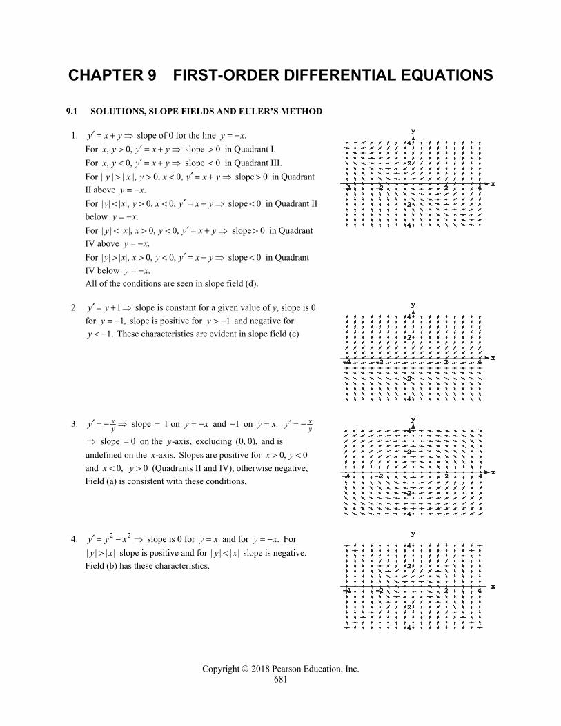
4. 2 2y y x slope is 0 for y x and for .y x For | | | |y x slope is positive and for | | | |y x slope is negative. Field (b) has these characteristics.

682 Chapter 9 First-Order Differential Equations

Copyright 2018 Pearson Education, Inc.

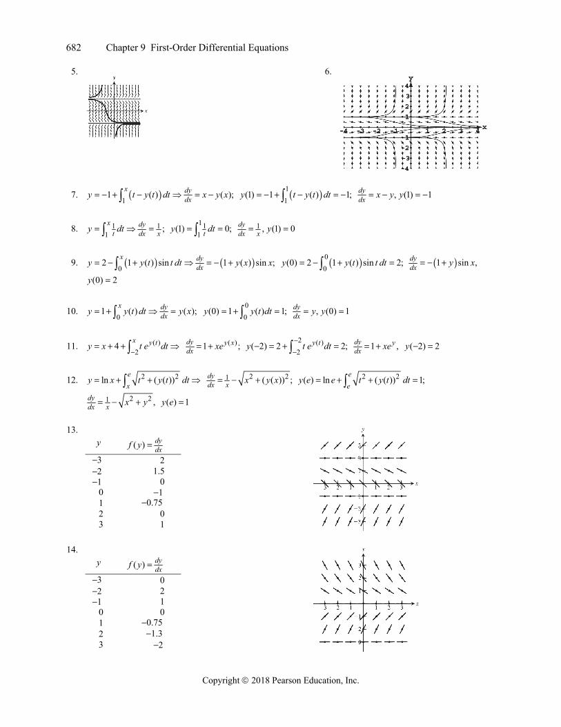
5.

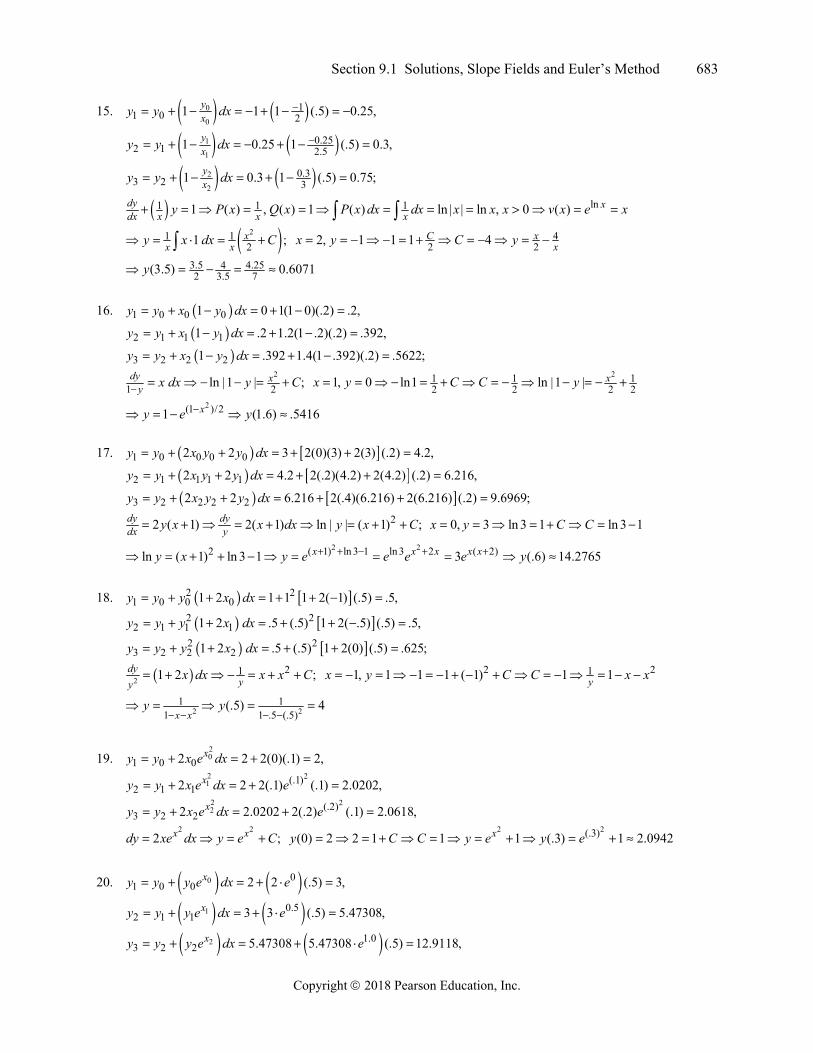
6.

7. 11 ( ) ( );

x dydxy t y t dt x y x 1

1(1) 1 ( ) 1;y t y t dt , (1) 1dy

dx x y y

8. 1 11

;x dy

t dx xy dt 111

(1) 0;ty dt 1 , (1) 0dydx x y

9. 02 1 ( ) sin 1 ( ) sin ;

x dydxy y t t dt y x x 0

0(0) 2 1 ( ) sin 2;y y t t dt 1 sin ,dy

dx y x

(0) 2y

10. 0

1 ( ) ( );x dy

dxy y t dt y x 00

(0) 1 ( ) 1;y y t dt , (0) 1dydx y y

11. ( )2

4 x y ty x t e dt

( )1 ;dy y xdx xe

2 ( )2

( 2) 2 2;y ty t e dt

1 ,dy ydx xe ( 2) 2y

12. 2 2ln ( ( )) ex

y x t y t dt 2 21 ( ( )) ;dydx x x y x 2 2( ) ln ( ( )) 1;

ee

y e e t y t dt

2 21 ,dydx x x y ( ) 1y e

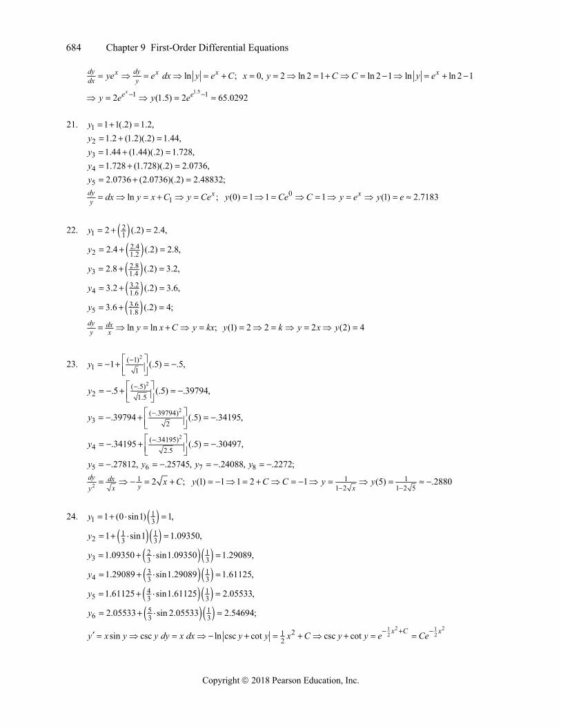
13. y ( ) dy

dxf y 3 2 2 1.5 1 0 0 1 1 0.75 2 0 3 1

14. y ( ) dy

dxf y 3 0 2 2 1 1 0 0 1 0.75 2 1.3 3 2

Section 9.1 Solutions, Slope Fields and Euler’s Method 683


15. 0

0

11 0 21 1 1 (.5) 0.25,y

xy y dx

1

1

0.252 1 2.51 0.25 1 (.5) 0.3,y

xy y dx

2

2

0.33 2 31 0.3 1 (.5) 0.75;y

xy y dx

ln1 1 11 ( ) , ( ) 1 ( ) ln | | ln , 0 ( )dy xdx x x xy P x Q x P x dx dx x x x v x e x

21 121 ;x

x xy x dx C 42 22, 1 1 1 4C x

xx y C y

3.5 4.2542 3.5 7(3.5) 0.6071y

16. 1 0 0 01 0 1(1 0)(.2) .2,y y x y dx

2 1 1 11 .2 1.2(1 .2)(.2) .392,y y x y dx

3 2 2 21 .392 1.4(1 .392)(.2) .5622;y y x y dx 2

1 2ln |1 | ;dy xy x dx y C

21 1 12 2 2 21, 0 ln1 ln |1 | xx y C C y

2(1 )/21 (1.6) .5416xy e y

17. 1 0 0 0 02 2 3 2(0)(3) 2(3) (.2) 4.2,y y x y y dx

2 1 1 1 12 2 4.2 2(.2)(4.2) 2(4.2) (.2) 6.216,y y x y y dx

3 2 2 2 22 2 6.216 2(.4)(6.216) 2(6.216) (.2) 9.6969;y y x y y dx 22 ( 1) 2( 1) ln | | ( 1) ;dy dy

dx yy x x dx y x C 0, 3 ln 3 1 ln 3 1x y C C 2 22 ( 1) ln 3 1 ln 3 2 ( 2)ln ( 1) ln 3 1 3 (.6) 14.2765x x x x xy x y e e e e y

18. 2 21 0 0 01 2 1 1 1 2( 1) (.5) .5,y y y x dx

2 22 1 1 11 2 .5 (.5) 1 2( .5) (.5) .5,y y y x dx

2 23 2 2 21 2 .5 (.5) 1 2(0) (.5) .625;y y y x dx

2211 2 ;dy

yyx dx x x C 2 211, 1 1 1 ( 1) 1 1yx y C C x x

2 21 1

1 1 .5 (.5)(.5) 4

x xy y

19. 201 0 02 2 2(0)(.1) 2,xy y x e dx 2 21 (.1)

2 1 12 2 2(.1) (.1) 2.0202,xy y x e dx e 2 22 (.2)

3 2 22 2.0202 2(.2) (.1) 2.0618,xy y x e dx e 2 2

2 ;x xdy xe dx y e C 2 2(.3)(0) 2 2 1 1 1 (.3) 1 2.0942xy C C y e y e

20. 0 01 0 0 2 2 (.5) 3,xy y y e dx e

1 0.52 1 1 3 3 (.5) 5.47308,xy y y e dx e

2 1.03 2 2 5.47308 5.47308 (.5) 12.9118,xy y y e dx e



ln ;dy dyx x xdx yye e dx y e C 0, 2 ln 2 1 ln 2 1 ln ln 2 1xx y C C y e

1.51 12 (1.5) 2 65.0292xe ey e y e

21. 1 1 1(.2) 1.2,y

2 1.2 (1.2)(.2) 1.44,y

3 1.44 (1.44)(.2) 1.728,y

4 1.728 (1.728)(.2) 2.0736,y

5 2.0736 (2.0736)(.2) 2.48832;y

1ln ;dy xy dx y x C y Ce 0(0) 1 1 1 (1) 2.7183xy Ce C y e y e

22. 21 12 (.2) 2.4,y

2.42 1.22.4 (.2) 2.8,y

2.83 1.42.8 (.2) 3.2,y

3.24 1.63.2 (.2) 3.6,y

3.65 1.83.6 (.2) 4;y

ln ln ;dy dxy x y x C y kx (1) 2 2 2 (2) 4y k y x y

23. 2( 1)

1 11 (.5) .5,y

2( .5)2 1.5

.5 (.5) .39794,y

2( .39794)3 2

.39794 (.5) .34195,y

2( .34195)4 2.5

.34195 (.5) .30497,y

5 6 7 8.27812, .25745, .24088, .2272;y y y y

21 2 ;dy dxyxy

x C 1 11 2 1 2 5

(1) 1 1 2 1 (5) .2880x

y C C y y

24. 11 31 (0 sin1) 1,y

1 12 3 31 sin1 1.09350,y

2 13 3 31.09350 sin1.09350 1.29089,y

3 14 3 31.29089 sin1.29089 1.61125,y

4 15 3 31.61125 sin1.61125 2.05533,y

5 16 3 32.05533 sin 2.05533 2.54694;y

2 21 12 221

2sin csc ln csc cot csc cot x C xy x y y dy x dx y y x C y y e Ce



2 21 12 21 cos

sin 2cot ;x xy yy Ce Ce 21

201 12 2 2(0) 1 cot cot cot xyy Ce C e

2121 1 21 1

2 22cot cot , (2) 2cot cot 2.65591xy e y e

25. 0 0 00 0 0 0 0 0 0 0 0 01 1 ( ) 1 1 1 1 (1)x x x xy x x y e y x x x y e x x y y

0 00 0 0 01 1 1 1dy dy dyx x x xdx dx dxx y e y x x y e x x y

26. 0

0 0( ), ( ) ( ) ,xx

y f x y x y y f t dt C 0

0 00 0 0( ) ( ) ( )

x xx x

y x f t dt C C C y y f t dt y

27–38. Example CAS commands: Maple:

ode : diff ( y(x), x ) y(x);

icA : [0,1];

icB : [0, 2];

icC : [0, -1];

DEplot( ode, y(x), x 0..2, [icA,icB,icC], arrows slim, linecolor blue, title " 27 (Section 9.1)" );#

Mathematica: To plot vector fields, you must begin by loading a graphics package. Graphics PlotField`

To control lengths and appearance of vectors, select the Help browser, type PlotVectorField and select Go. Clear[x, y, f ] yprime y (2 y);

pv PlotVectorField[{1, yprime}, {x, 5, 5}, {y, 4, 6}, Axes True, AxesLabel {x, y}]; To draw solution curves with Mathematica, you must first solve the differential equation. This will be done with the DSolve command. The y[x] and x at the end of the command specify the dependent and independent variables. The command will not work unless the y in the differential equation is referenced as y[x].

equation y'[x] y[x] (2 y[x]) ;

initcond y[a] b;

sols DSolve[{equation, initcond}, y[x], x]

vals {{0, 1/2}, {0, 3/2}, {0, 2}, {0, 3}}

_ _f[{a , b }] sols[[1, 1, 2]];

solnset Map[f, vals]

ps Plot[Evaluate[solnset, {x, 5, 5}];

Show[pv, ps, PlotRange { 4, 6}]; The code for problems such as 35 & 36 is similar for the direction field, but the analytical solutions involve complicated inverse functions, so the numerical solver NDSolve is used. Note that a domain interval is specified.

equation y'[x] Cos[2x y[x]] ;



initcond y[0] 2;

sol NDSolve[{equation, initcond}, y[x], {x, 0, 5}]

ps Plot[Evaluate[y[x]/.sol, {x, 0, 5}];

N[y[x] /. sol/.x 2]

Show[pv, ps, PlotRange {0, 5}]; Solutions for 37 can be found one at a time and plots named and shown together. No direction fields here. For 38, the direction field code is similar, but the solution is found implicitly using integrations. The plot requires loading another special graphics package.

Graphics ImplicitPlot`

Clear[x,y]

2_solution[c ] Integrate[2 (y 1), y] Integrate[3x 4x 2, x] c

values { 6, 4, 2, 0, 2, 4, 6};

solns Map[solution, values];

ps ImplicitPlot[solns, {x, 3, 3}, {y, 3, 3}]

Show[pv, ps]

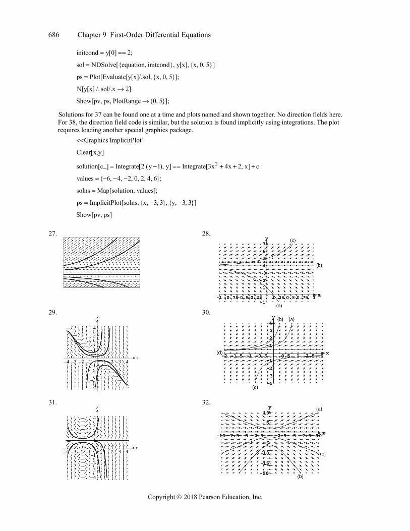
27.

28.

29.

30.

31.

32.



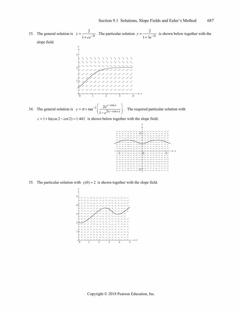
33. The general solution is 22

1 tyce

. The particular solution 22

1 3 tye

is shown below together with the

slope field.

0 1 2 3 4

1

2

3

x

y

34. The general solution is cos

12( cos )

2tan1

c x

c xeye

. The required particular solution with

1 ln(csc 2 cot 2) 1.443c is shown below together with the slope field.

5 0 5

5

5

x

y

35. The particular solution with (0) 2y is shown together with the slope field.

0 1 2 3 4 5

1

2

3

4

5

x

y



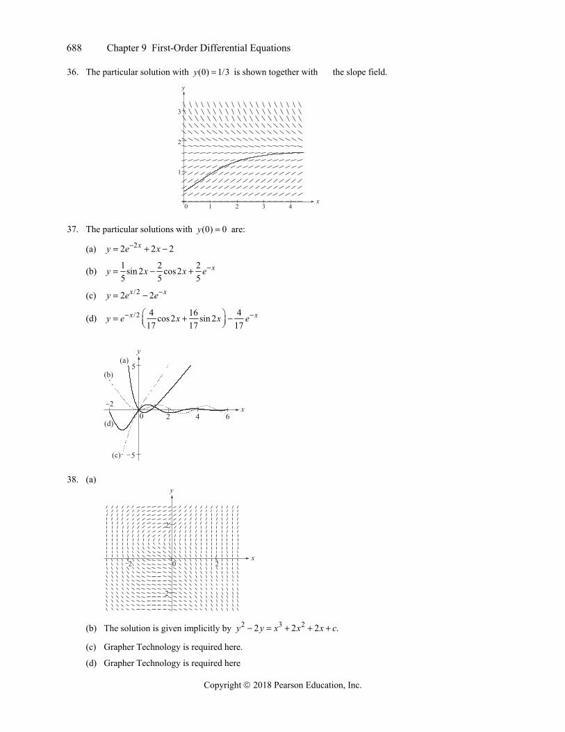
36. The particular solution with (0) 1/3y is shown together with the slope field.

0 1 2 3 4

1

2

3

x

y

37. The particular solutions with (0) 0y are:

(a) 22 2 2xy e x

(b) 1 2 2sin 2 cos25 5 5

xy x x e

(c) /22 2x xy e e

(d) /2 4 16 4cos2 sin 217 17 17

x xy e x x e

20 2 4 6

5

5

x

y(a)

(b)

(c)

(d)

38. (a)

2 0 2

2

2

x

y

(b) The solution is given implicitly by 2 3 22 2 2 .y y x x x c (c) Grapher Technology is required here.

(d) Grapher Technology is required here



39. 2 2 22

12 , (0) 2 2 2 (0.1) 0.2n n ndy x x xxn n n n n n ndx xe y y y x e dx y x e y x e

On a TI-84 calculator home screen, type the following commands: 2 STO y: 0 STO x: y (enter) y 0.2*x*e^(x^2)STO y: x 0.1STO x: y (enter, 10 times) The last value displayed gives Eulery (1) 3.45835

The exact solution: 2 2

2 ;x xdy xe dx y e C 20(0) 2 1 1 xy e C C y e

exact (1) 1 3.71828y e

40. 22 ( 1),dydx y x 2 21

12(2) 2 1 0.2 1n n n n n n ny y y y x dx y y x On a TI-84 calculator home screen, type the following commands:

0.5 STO y : 2 STO x: y (enter) 2y 0.2*y (x 1) STO y: x 0.1STO x: y (enter, 10 times)

The last value displayed gives Euley (2) 0.19285r

The exact solution: 22 2 21 12 ( 1) (2 2) 2 2dy dy

dx y yyy x x dx x x C x x C

22 21 1 1 1

2 1/2 2 2(2) (2) 2(2) 2 2 2y x x

y C C C x x y

21

(3) 2(3) 2(3) 0.2y

41. 1, 0, (0) 1 (0.1) 0.1n n n

n n n

x x xdy xn n n ndx y y y yy y y y dx y y

On a TI-84 calculator home screen, type the following commands: 1STO y: 0 STO x: y (enter)

y 0.1*( x /y) STO y: x 0.1STO x: y (enter, 10 times) The last value displayed gives Eulery (1) 1.5000

The exact solution: 2 3/22

2 3 ;yxydy dx y dy x dx x C 2 2(0) 3/21 1 2 1

2 2 2 3 2(0)y C C 2 3/2 3/2 3/22 1 4 4

exact2 3 2 3 31 (1) (1) 1 1.5275y x y x y

42. 21 ,dydx y 2 2 2

1(0) 0 1 1 (0.1) 0.1 1n n n n n n ny y y y dx y y y y

On a TI-84 calculator home screen, type the following commands: 0 STO y: 0 STO x: y (enter)

2y 0.1*(1 y ) STO y: x 0.1STO x: y (enter, 10 times) The last value displayed gives Eulery (1) 1.3964

The exact solution: 22 1

11 tan ;dy

ydy y dx dx y x C

1 1tan (0) tan 0 0 0y C

1exact0 tan tan (1) tan1 1.5574C y x y x y

43. Example CAS commands: Maple:

ode : diff ( y(x), x ) x y(x);ic : y(0) -7/10;

x0 : -4;x1: 4;y0 : -4; y1: 4;



b : 1;

P1: DEplot( ode, y(x), x x0..x1, y y0..y1, arrows thin, title "#43(a) (Section 9.1)" ):

P1;

_Ygen : unapply( rhs(dsolve( ode, y(x) )), x, C1 ); # (b)

P2 : seq( plot( Ygen(x,c), x x0..x1, y y0..y1, color blue ), c -2..2 ): # (c)

display( [P1,P2], title "#43(c) (Section 9.1)" );

CC : solve( Ygen(0,C) rhs(ic), C); # (d)

Ypart : Ygen(x,CC);

P3: plot( Ypart, x 0..b, title "#43(d) (Section 9.1)" ):

P3;

euler4 : dsolve( {ode,ic}, numeric, method classical[foreuler], stepsize (x1-x0)/4 ): # (e)

P4 : odeplot( euler4, [x,y(x)], x 0..b, numpoints 4, color blue ):

display( [P3,P4], title " 43(e) (Section 9. ;# 1)" )

euler8 : dsolve( {ode,ic}, numeric, method classical[foreuler], stepsize (x1-x0)/8 ): # (f )

odeplot( euler8, [x,y(x)], x 0..b, numpoints 8, color green ): :P5

eulerl6 : dsolve( {ode,ic},numeric, method classical[foreuler], stepsize (x1-x0)/16 ):

P6 : odeplot( euler16, [x,y(x)], x 0..b, numpoints 16, color pink ):

euler32 : dsolve( {ode,ic},numeric, method classical[foreuler], stepsize (x1-x0)/32 ):

P7 : odeplot( euler32, [x,y(x)], x 0..b, numpoints 32, color cyan ):

display( [P3,P4,P5,P6,P7], title "#43(f ) (Section 9.1)" );

N | h |`percent error` , # (g)

4 | (x1-x0)/ 4 | evalf[5]( abs(1-eval(y(x),euler4(b))/eval(Ypart, x b))*100 ) ,

8 | (x1-x0)/ 8 | evalf[5]( abs(1-eval(y(x),euler8(b))/eval(Ypart, x b))*100 ) ,

16 | (x1-x0)/16 | evalf[5]( abs(1-eval(y(x),euler16(b))/eval(Ypart, x b))*100 ) ,

32 | (x1-x0)/ 32 | evalf[5]( abs(1-eval(y(x),euler32(b))/eval(Ypart, x b))*100 ) ;

43–46. Example CAS commands: Mathematica: (assigned functions, step sizes, and values for initial conditions may vary) Problems 43–46 involve use of code from Problems 27–38 together with the above code for Euler’s method.

9.2 FIRST-ORDER LINEAR EQUATIONS

1. 1 ,xdy dyx e

dx dx x xx y e y 1( ) , ( )xe

x xP x Q x

( ) ln1( ) ln | | ln , 0 ( ) P x dx xxP x dx dx x x x v x e e x

1 1 1( ) ( ) ( ) , 0

x xxe e Cv x x x x xy v x Q x dx x dx e C x

Section 9.2 First-Order Linear Equations 691


2. 2 1 2 ,dy dyx x xdx dxe e y y e ( ) 2, ( ) xP x Q x e

( ) 2( ) 2 2 ( ) P x dx xP x dx dx x v x e e

2 2 22 21 1 1

x x xx x x x x x

e e ey e e dx e dx e C e Ce

3. 2 3sin 3 sin3 , 0 ,dyx x

dx xx xxy y x y 3

3 sin( ) , ( ) xx x

P x Q x 33 ln 33 3ln ln , 0 ( ) x

x dx x x x v x e x

3 3 3 3 33 sin cos1 1 1sin cos , 0x C x

x x x x xy x dx x dx x C x

4. 2 22 2tan cos , tan cos ,dy

dxy x y x x x y x 2( ) tan , ( ) cosP x x Q x x 11 ln(cos ) 1sin

cos 2 2tan ln | cos | ln (cos ) , ( ) (cos ) secxxxx dx dx x x x v x e x x

21sec sec cos (cos ) cos (cos ) sin sin cos cosxy x x dx x x dx x x C x x C x

5. 21 2 1 12 1 , 0 ,dy dy

dx x dx x x xx y x y 2

2 1 1( ) , ( )x x xP x Q x

22 ln 22 2ln ln , 0 ( ) xx dx x x x v x e x

2

2 2 2 2 221 1 1 1 1 1 1

2 2( 1) , 0x Cx xx x x x x

y x dx x dx x C x

6. 11 1(1 ) ,dy x

dx x xx y y x y 1

1 1( ) , ( ) xx xP x Q x

11 ln(1 ),x dx x since ln(1 )0 ( ) 1xx v x e

3/23/2 21 1 1 21 1 1 1 3 3(1 ) 1(1 ) x x C

x x x x x xy x dx x dx x C

7. /21 1 12 2 2( ) ,dy x

dx y e P x /2 /21 12 2( ) ( ) ( )x xQ x e P x dx x v x e

/2/2 /2 /2 /2 /2 /21 1 1 1 1

2 2 2 2xx x x x x x

ey e e dx e dx e x C xe Ce

8. 22 2 ( ) 2,dy xdx y xe P x 2 2( ) 2 ( ) 2 2 ( )x xQ x xe P x dx dx x v x e

2 22 2 2 2 2 2 21 12 2x x

x x x x xe e

y e xe dx x dx e x C x e Ce

9. 1 12ln ( ) ,dydx x xy x P x 1( ) 2 ln ( ) ln , 0xQ x x P x dx dx x x

2 2ln 1 1( ) 2 ln ln lnxx xv x e y x x dx x x C x x Cx

10. 2cos2 2, 0 ( ) ,dy x

dx x xxy x P x 2

2cos 2( ) ( ) 2ln ln , 0xxx

Q x P x dx dx x x x

2

2 2 2 2 2ln 2 2 cos sin1 1 1( ) cos sinx x x C

x x x x xv x e x y x dx x dx x C



11. 314 4

1 1( 1)( ) ,ds t

dt t tts P t

3

41 41( 1)

( ) ( ) 4 ln 1 ln ( 1)ttt

Q t P t dt dt t t

4 3

4 3 4 4ln( 1) 4 4 211 1 1

3( 1) ( 1) ( 1) ( 1)( ) ( 1) ( 1) 1t t t

t t t tv t e t s t dt t dt t C

3

4 4 43( 1) ( 1) ( 1)t t C

t t t

12. 2 31 2 1 2

1 1( 1) ( 1)( 1) 2 3( 1) 3 ( ) ,ds ds

dt dt t tt tt s t s P t 3( ) 3 ( 1)Q t t

22 ln ( 1) 221( ) 2 ln 1 ln ( 1) ( ) ( 1)t

tP t dt dt t t v t e t

2 22 3 2 11 1

( 1) ( 1)( 1) 3 ( 1) 3( 1) ( 1)

t ts t t dt t t dt

2 23 21

( 1) ( 1)( 1) ln 1 ( 1) ( 1) ln ( 1) , 1C

t tt t C t t t t

13. (cot ) sec ( ) cot ,drd r P ln |sin |( ) sec ( ) cot ln |sin | ( )Q P d d v e

sin because 1 1 12 sin sin sin0 (sin )(sec ) tan ln |sec |r d d C

(csc ) ln |sec | C

14. 22 sin

tan tantan sin (cot ) sin cos ( ) cot ,dr dr drrd d dr r P ( ) sin cosQ

( ) cot ln sin ln(sin )P d d since ln(sin )20 ( ) sinv e

3 22 sin sin1 1 1sin sin sin 3 3 sin(sin )(sin cos ) sin cos Cr d d C

15. 2 3 ( ) 2,dydt y P t 2 2

2 2 231 12( ) 3 ( ) 2 2 ( ) 3 ;t t

t t te e

Q t P t dt dt t v t e y e dt e C

23 31 12 2 2 2(0) 1 1 ty C C y e

16. 2 2 2( ) ,dy ydt t tt P t 2

22 ln 2 2 21( ) ( ) 2 ln | | ( ) t

tQ t t P t dt t v t e t y t t dt

5 3

2 2 241 1

5 5 ;t t Ct t t

t dt C 3

28 12 125 4 5 5 5

(2) 1 1C tt

y C y

17. sin1 1( ) ,dyd y P ln| |sin sin1

| |( ) ( ) ln ( )Q P d v e y d

sin1 d for 1 1 10 sin cos cos ;Cy d C 2 21y C

12cosy

18. 22 2sec tan ( ) ,dyd y P 2 2ln| |( ) sec tan ( ) 2 ln | | ( )Q P d v e

22 2 2 2 2 2 21 sec tan sec tan sec sec ;y d d C C

2 2

2 22 218 18

3 9 92 2 (2) 2 sec 2y C C y

Section 9.2 First-Order Linear Equations 693


19. 2 2 2

2 2( 1)2

1 1 ( 1) ( 1)( 1) 2 2 2 ( ) 2 ,

x x xdy dy x x dye e edx x dx x dxx x

x x x y y xy P x x

2

2( 1)( )

xex

Q x

2 12 2 2 2

2 2 2( 1)2 1 1

1( 1) ( 1)( ) 2 ( )

x

x

xx x x xex xe

P x dx x dx x v x e y e dx e dx e C

2 2

1 ;x xe

x Ce 221

0 1 1(0) 5 5 1 5 6 6xx e

xy C C C y e

20. ( ) ,dydx xy x P x x

2 22

2 /2

/2 /212( ) ( ) ( )

x

x xxe

Q x x P x dx x dx v x e y e x dx

2

2 2/2 /2

/21 1 ;x x

x Ce e

e C 2 /27(0) 6 1 6 7 1

xey C C y

21. 0 ( ) ,dydt ky P t k 1( ) 0 ( ) ( ) (0)kt

kt kte

Q t P t dt k dt kt v t e y e dt

(0 ) ;kt kte C Ce 0 0 0(0) kty y C y y y e

22. (a) 0 ( ) ,du k kdt m mu P t /( ) 0 ( ) ( ) kt mk k kt

m m mQ t P t dt dt t u t e

/ //1 0 ;kt m kt m

kt m Ce e

y e dt (0)/( / )

0 0 0 0(0) k mk m tC

eu u u C u u u e

(b) ( / ) ( / )ln .k m t C k m t Cdu k du k kdt m u m mu dt u t C u e u e e Let 1.Ce C

Then ( / )1

1k m teu C and ( / )(0)

10 1 1(0) .k me

u u C C So ( / )0

k m tu u e

23. 1 ln ln | |xx dx x x C x x Cx (b) is correct

24. 1 1cos cos coscos sin tan C

x x xx dx x C x (b) is correct

25. Steady State VR and we want / / /1 1 1 1

2 2 2 21 1Rt L Rt L Rt LV V VR R Ri e e e

1 12 2ln ln ln 2Rt L L

L R Rt t sec

26. (a) 1 / /110 ln ;C Rt L Rt Ldi RtR R

dt L i L Li di dt i C i e e Ce (0)i I I C /Rt Li Ie amp

(b) / /1 1 12 2 2ln ln 2 ln 2Rt L Rt L Rt L

L RI I e e t .sec

(c) ( / )( / )Rt L L R tLRt i I e I e amp

27. (a) ( / )(3 / ) 33 1 1 0.9502R L L RL V V VR R R Rt i e e amp, or about 95% of the steady state value

(b) ( / )(2 / ) 22 1 1 0.8647R L L RV V VLR R R Rt i e e amp or about 86% of the steady state value

28. (a) ( ) ,di VR Rdt L L Li P t /

/ /1( ) ( ) ( ) Rt LRt L Rt LV Rt VR

L L L LeQ t P t dt dt v t e i e dt

// ( / )1

Rt LRt L R L tV VL

R L Ree C Ce



(b) /(0) 0 0 Rt LV V V VR R R Ri C C i e

(c) 0 0V di di V V VR RR dt dt L L R L Ri i i is a solution of Eq. (6); ( / )R L ti Ce

29. 2;y y y we have 2,n so let 1 2 1.u y y Then 1y u and 2 21 dy dydu dudx dx dx dxy y

2 1 2 1.du dudx dxu u u u With dx xe e as the integrating factor, we have

.x x xdu ddx dxe u e u e Integrating, we get 1 1

11

x

x C xxe

x x C eye e C

e u e C u y

30. 2;y y xy we have 2,n so let 1.u y Then 1y u and 2 2 2 .dy dydu du dudx dx dx dx dxy y u

Substituting: 2 1 2 .du dudx dxu u xu u x Using dx xe e as an integrating factor:

(1 ) 1(1 )x x

x x xe x Cx x x x xdu d e

dx dx e e xe Ce u e u x e e u e x C u y u

31. 2 21 1 .x xxy y y y y y Let 1 ( 2) 3 1/3u y y y u and 2 2/3.y u

2 2 2/31 13 33 .dy dydu du du

dx dx dx dx dxy y y u Thus we have

2/3 1/3 2/3 3 31 1 13 .du du

dx x x dx x xu u u u The integrating factor is 3 3ln( ) x dx xv x e e

3ln 3.xe x Thus 3 3

1/33 3 2 3 3 33 3 1 1d C Cdx x x x

x u x x x u x C u y y

32. 22 3 32 12 .x x

x y xy y y y y 22 1( ) , ( ) , 3.x x

P x Q x n Let 1 3 2.u y y Substituting

gives 2 22 1 4 2( 2) 2 .du du

dx x dx xx xu u Let the integrating factor, ( ),v x be

4 4ln 4.x dx xe e x Thus 4 6 4 5 4 22 2

5 52ddx xx u x x u x C u Cx y

1/2425xy Cx

9.3 APPLICATIONS

1. Note that the total mass is 66 7 73 kg, therefore, ( / ) 3.9 /730 9k m t tv v e v e

(a) 3.9 /73 3.9 /73219013( ) 9 t ts t e dt e C

Since (0) 0s we have 219013C and 3.9 /732190 2190

13 13lim ( ) lim 1 168.5tt t

s t e

The cyclist will coast about 168.5 meters. (b) 3.9/73 3.9 73ln 9

73 3.91 9 ln 9 41.13te t sec It will take about 41.13 seconds.

Section 9.3 Applications 695


2. ( / ) (59,000/51,000,000) 59 /51,0000 9 9k m t t tv v e v e v e

(a) 459,00059 /51,000 59 /51,00059( ) 9 t ts t e dt e C

Since (0) 0s we have 459,00059C and 459,000 459,00059 /51,000

59 59lim ( ) lim 1 7780tt t

s t e

m

The ship sill coast about 7780 m, or 7.78 km. (b) 51,000ln 959 /51,000 59

51,000 591 9 ln 9 1899.3t te t sec

It will take about 31.65 minutes.

3. The total distance traveled 0 (2.75)(39.92) 4.91 22.36.v mk k k Therefore, the distance traveled is given

by the function (22.36/39.92)( ) 4.91 1 .ts t e The graph shows ( )s t and the data points.

4. 0v mk coasting distance (0.80)(49.90) 998

331.32k k

We know that 0 1.32v mk and 998 20

33(49.9) 33 .km

Using Equation 2, we have: 0 ( / ) 20 /33 0.606( ) 1 1.32 1 1.32 1v m k m t t tks t e e e

5. 2 0 .y xy y yx xx

y mx m y So for

orthogonals: 2 2

2 2dy yx xdx y y dy x dx C

2 21x y C

6. 2

2 422 20 2y x y xy

x xy cx c x y xy

2 .yxy So for the orthogonals: 2

dy xdx y

2 222 22 ,x xydy xdx y C y C

0C



7. 2

212 2 2 21 1 y

xkx y y kx k

2 2

4

(2 ) 1 2 2 20 2 1 (2 )x y y y x

xyx y y x

2 2

2

1 (2 ) 1

2.

y x y

xyxyy

So for the orthogonals:

2 2 2

2

12 21

lnydy xy y x

dx yydy x dx y C

8. 2 2 2 4 222 4 2 0 .x x

y yx y c x yy y For

orthogonals: 12 2 2ln lndy y dy dx

dx x y x y x C

1/2 1/21 1ln ln ln | |y x C y C x

9.

2( 1)

0x x

x x

e y y eyxe e

y ce c

.x xe y ye y y So for the orthogonals: 2 21

12 2dy ydx y y dy dx x C y x C

12y x C

10. 1

2

lnlnln 0yx y yykxx x

y e y kx k

lnln 0 .y yxy xy y y So for the

orthogonals: ln lndy xdx y y y y dy x dx

2 2 21 1 12 4 2lny y y x C

22 212ln yy y x C

11. 2 22 3 5x y and 2 3y x intersect at (1, 1). Also, 2 2 462 3 5 4 6 0 x

yx y x y y y

23(1,1)y and

2

1

2 3 2 3 31 1 1 1 12 22 3 (1, 1) .x

yy x y y x y y Since 321 3 2 1,y y the

curves are orthogonal.

Section 9.3 Applications 697


12. (a) 22

2 20 yxx dx y dy C the general

equation of the family with slope .xyy

For the orthogonals: y dy dxx y xy

ln lny x C or 1y C x (where 1CC e )

is the general equation of the orthogonals.

(b) 22 0 2 dy dx

y xx dy y dx y dx x dy

21 112 2 ln lndy dx

y x y x C y C x

is the equation for the solution family. 21 1 1

2 2ln ln 0y yy x xy x C y

slope of orthogonals is 2dy xdx y

2222 xy dy x dx y C is the

general equation of the orthogonals.

13. Let ( )y t the amount of salt in the container and ( )V t the total volume of liquid in the tank at time t. Then,

the departure rate is ( )( )

y tV t (the outflow rate).

(a) Rate entering gallb lbgal min min2 5 10

(b) Volume ( ) 100 gal (5 gal 4 gal) (100 )galV t t t t (c) The volume at time t is (100 )t gal. The amount of salt in the tank at time t is y lbs. So the concentration

at any time t is lb100 gal .y

t Then, the rate leaving gal 4lb lb100 gal min 100 min4y y

t t

(d) 4 4 4100 100 10010 10 ( ) ,dy y dy

dt t dt t ty P t 4100( ) 10 ( ) 4ln (100 )tQ t P t dt dt t

5

4 4(100 )4ln (100 ) 4 4 101

5(100 ) (100 )( ) (100 ) (100 ) (10 ) tt

t tv t e t y t dt C

4(100 )2(100 ) ;C

tt

4

4(100 0)

(0) 50 2(100 0) 50 (150)(100)Cy C

4

4 4100

(150)(100) 150(100 ) 1

2(100 ) 2(100 )tt

y t y t

(e) 4

4(150)(100) (25) 188.6 lb

volume 125 gal(100 25)(25) 2(100 25) 188.56 lbs concentration 1.5yy

14. (a) (5 3) 2 100 2dVdt V t

The tank is full when 200 100 2 50minV t t



(b) Let ( )y t be the amount of concentrate in the tank at time t.

gal gallb lb 5 3 3 512 gal min 100 2 gal min 2 2 50 2( 50) 25 3dy y dy y dy

dt t dt t dt t y 52( ) ;Q t

3 3 31 12 50 2 50 2( ) ( ) ln ( 50)t tP t P t dt dt t since 50 0t

32 ln ( 50)( )( ) tP t dtv t e e

3/2 3/23/2 3/2 3/2 5/251

2( 50) ( 50)( 50) ( ) ( 50) ( 50) ( 50) ( ) 50 C

t tt y t t dt t t C y t t

Apply the initial condition (i.e., distilled water in the tank at 0t ): 5/2

3/2 3/25/2 50

50 ( 50)(0) 0 50 50 ( ) 50 .C

ty C y t t

When the tank is full at = 50,t

5/2

3/250

100(50) 100 83.22y pounds of concentrate.

15. Let y be the amount of fertilizer in the tank at time t. Then rate entering gallb lbgal min min1 1 1 and the volume

in the tank at time t is gal galmin min( ) 100 (gal) 1 3 min (100 2 ) gal.V t t t

Hence rate out

3 3lb lb 3 3100 2 100 2 min 100 2 min 100 2 100 23 1 1 ( ) ,y y dy y dy

t t dt t dt t ty P t ( ) 1Q t

3ln(100 2 ) 3ln(100 2 ) /2 3/23100 2 2( ) ( ) (100 2 )t t

tP t dt dt v t e t

1/2

3/22(100 2 )3/2 3/2 3/21

2(100 2 )(100 2 ) (100 2 ) (100 2 ) (100 2 ) ;t

ty t dt t C t C t

3/2 3/2 1/2 110(0) 0 100 2(0) 100 2(0) (100) 100 (100)y C C C

3/2(100 2 )10(100 2 ) .ty t Let 1/23

2 (100 2 ) ( 2) 3 100 210 100 2 2 0

tdy dy tdt dt

20 3 100 2 400 9(100 2 ) 400 900 18 500 18 27.8min,t t t t t the time to

reach the maximum. The maximum amount is then 3/2100 2(27.8)10(27.8) 100 2(27.8) 14.8 lby

16. Let ( )y y t be the amount of carbon monoxide (CO) in the room at time t. The amount of CO entering the

room is 33 ft4 12100 10 1000 min, and the amount of CO leaving the room is 33 ft

4500 10 15,000 min .y y

Thus, 12 1 12 11000 15,000 15,000 1000 15,000( ) ,dy y dy

dt dt y P t /15,000121000( ) ( ) tQ t v t e

/15,0001215,000/15,000 /15,000 /15,000 /15,000 /15,0001 12

1000 1000 180 ;tt t t t t

ey e dt y e e C e e C

/15,000(0) 0 0 1(180 ) 180 180 180 .ty C C y e When the concentration of CO is 0.01%

in the room, the amount of CO satisfies 3.014500 100 0.45 ft .y y When the room contains this amount

we have /15,000 /15,000179.55 179.55180 1800.45 180 180 15,000ln 37.55min .t te e t

Section 9.4 Graphical Solutions of Autonomous Equations 699


9.4 GRAPHICAL SOLUTIONS OF AUTONOMOUS EQUATIONS

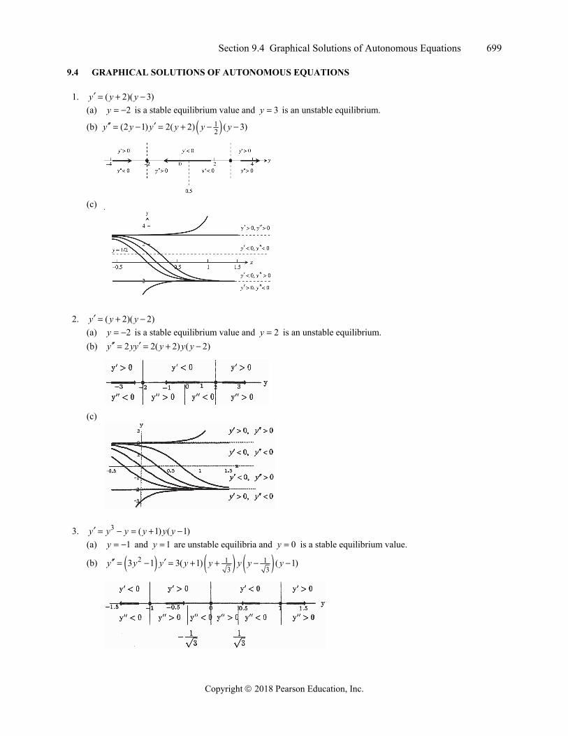
1. ( 2)( 3)y y y (a) 2y is a stable equilibrium value and 3y is an unstable equilibrium.

(b) 12(2 1) 2( 2) ( 3)y y y y y y

(c)

2. ( 2)( 2)y y y (a) 2y is a stable equilibrium value and 2y is an unstable equilibrium. (b) 2 2( 2) ( 2)y yy y y y

(c)

3. 3 ( 1) ( 1)y y y y y y (a) 1y and 1y are unstable equilibria and 0y is a stable equilibrium value.

(b) 2 1 13 3

3 1 3( 1) ( 1)y y y y y y y y



(c)

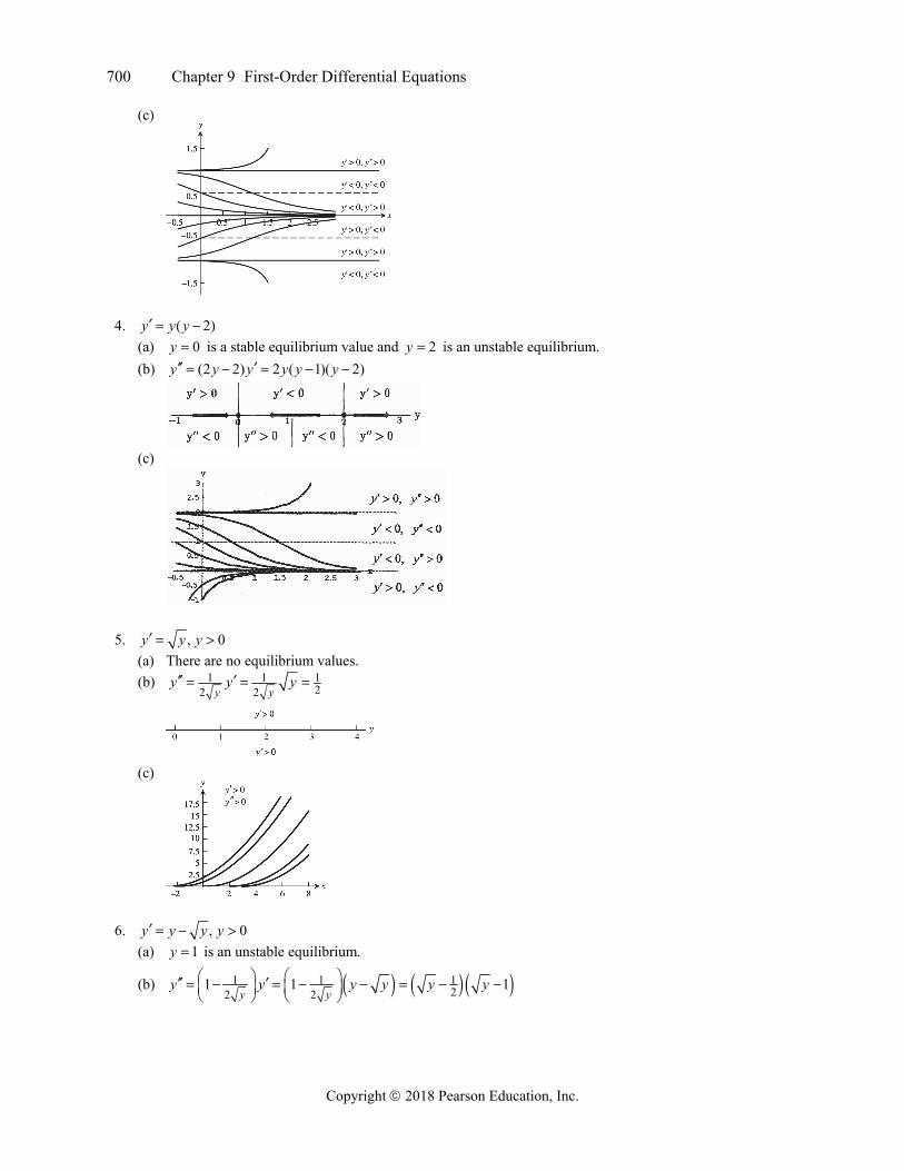
4. ( 2)y y y (a) 0y is a stable equilibrium value and 2y is an unstable equilibrium. (b) (2 2) 2 ( 1)( 2)y y y y y y

(c)

5. , 0y y y (a) There are no equilibrium values. (b) 1 1 1

22 2y yy y y

(c)

6. , 0y y y y (a) 1y is an unstable equilibrium.

(b) 1 1 122 2

1 1 1y y

y y y y y y



(c)

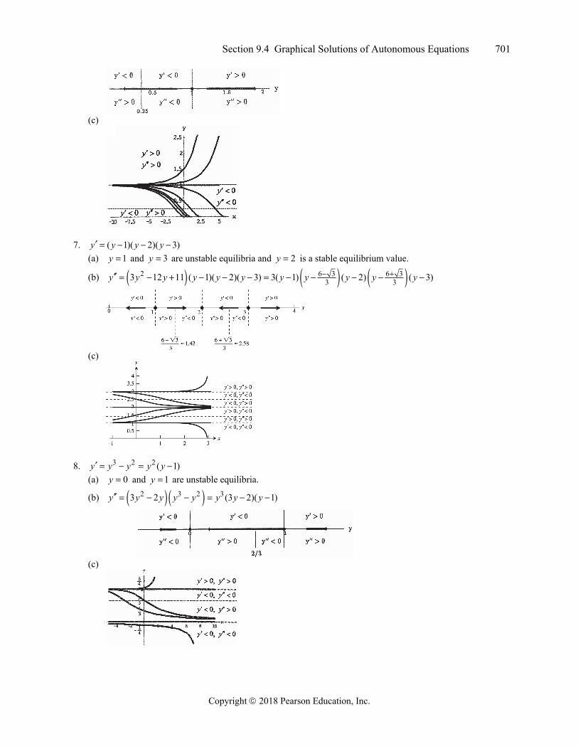
7. ( 1)( 2)( 3)y y y y (a) 1y and 3y are unstable equilibria and 2y is a stable equilibrium value.

(b) 2 6 3 6 33 33 12 11 ( 1)( 2)( 3) 3( 1) ( 2) ( 3)y y y y y y y y y y y

(c)

8. 3 2 2 ( 1)y y y y y (a) 0y and 1y are unstable equilibria.

(b) 2 3 2 33 2 (3 2)( 1)y y y y y y y y

(c)



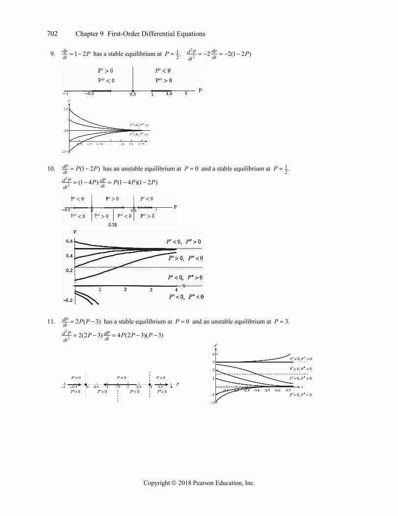
9. 1 2dpdt P has a stable equilibrium at 1

2 .P 2

2 2 2(1 2 )dpd Pdtdt

P

10. (1 2 )dPdt P P has an unstable equilibrium at 0P and a stable equilibrium at 1

2 .P 2

2 (1 4 ) (1 4 )(1 2 )d P dPdtdt

P P P P

11. 2 ( 3)dPdt P P has a stable equilibrium at 0P and an unstable equilibrium at 3.P

2

2 2(2 3) 4 (2 3)( 3)d P dPdtdt

P P P P



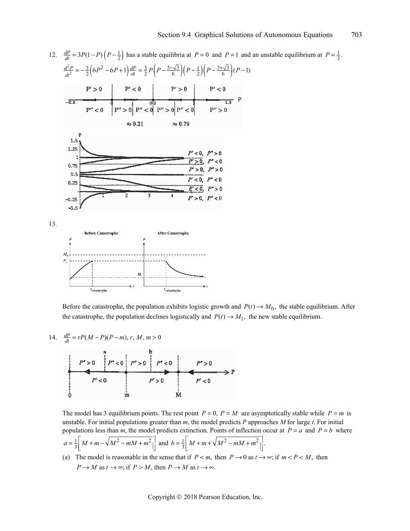
12. 123 (1 )dP

dt P P P has a stable equilibria at 0P and 1P and an unstable equilibrium at 12 .P

2

22 3 3 3 33 3 1

2 2 6 2 66 6 1 ( 1)d P dPdtdt

P P P P P P P

13.

Before the catastrophe, the population exhibits logistic growth and 0( ) ,P t M the stable equilibrium. After the catastrophe, the population declines logistically and 1( ) ,P t M the new stable equilibrium.

14. ( )( ), , , 0dPdt rP M P P m r M m

The model has 3 equilibrium points. The rest point 0, P P M are asymptotically stable while P m is unstable. For initial populations greater than m, the model predicts P approaches M for large t. For initial populations less than m, the model predicts extinction. Points of inflection occur at P a and P b where

2 213a M m M mM m

and 2 213 .b M m M mM m

(a) The model is reasonable in the sense that if ,P m then 0 as ; if ,P t m P M then as ; if , then as .P M t P M P M t



(b) It is different if the population falls below m, for then 0P as t (extinction). It is probably a more realistic model for that reason because we know some populations have become extinct after the population level became too low.

(c) For P M we see that ( ) ( )dPdt rP M P P m is negative. Thus the curve is everywhere decreasing.

Moreover, P M is a solution to the differential equation. Since the equation satisfies the existence and uniqueness conditions, solution trajectories cannot cross. Thus, as .P M t

(d) See the initial discussion above. (e) See the initial discussion above.

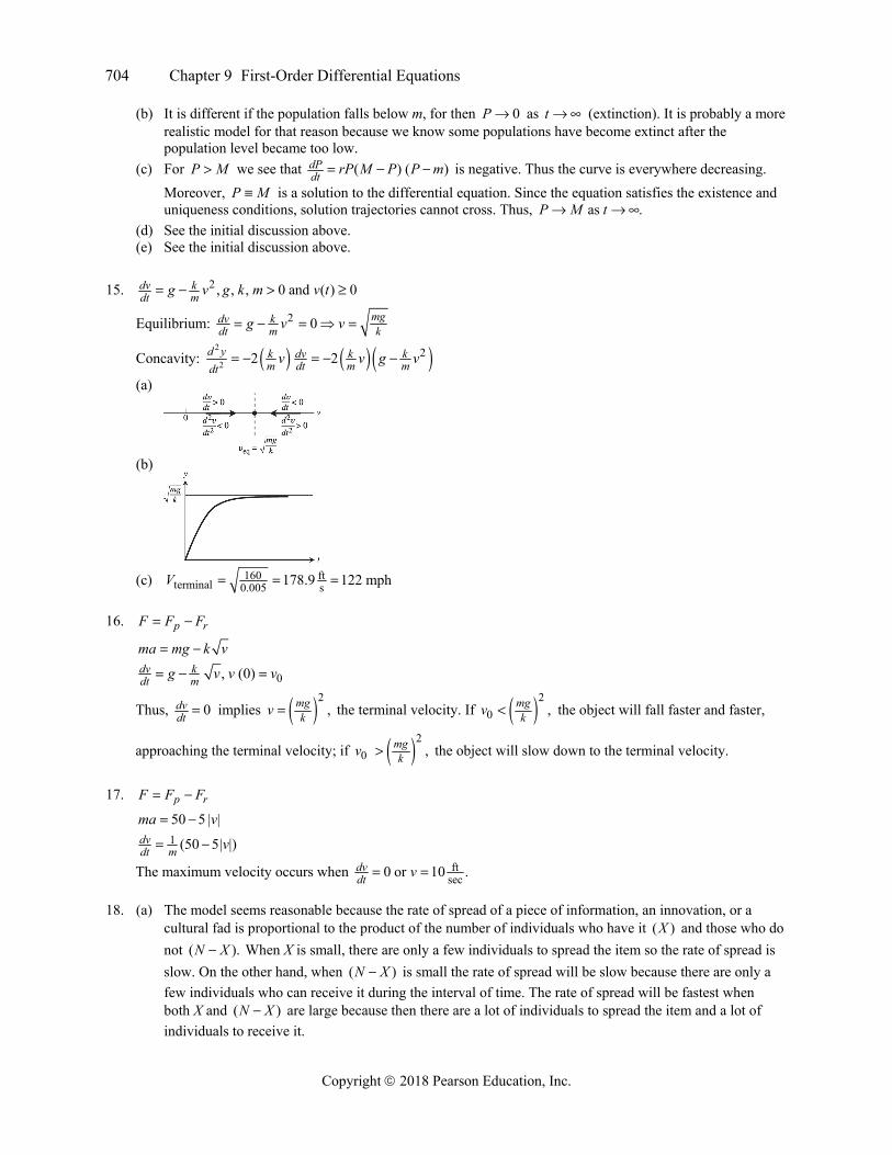
15. 2 , , , 0 and ( ) 0dv kdt mg v g k m v t

Equilibrium: 2 0 mgdv kdt m kg v v

Concavity: 2

222 2d y k dv k k

m dt m mdtv v g v

(a)

(b)

(c) 160 ft

terminal 0.005 s178.9 122 mphV

16. p rF F F

ma mg k v

0, (0)dv kdt mg v v v

Thus, 0dvdt implies 2 ,mg

kv the terminal velocity. If 20 ,mgkv the object will fall faster and faster,

approaching the terminal velocity; if 20 ,mgkv the object will slow down to the terminal velocity.

17. p rF F F

50 5 | |ma v 1 (50 5| |)dv

dt m v

The maximum velocity occurs when ftsec0 or 10 .dv

dt v

18. (a) The model seems reasonable because the rate of spread of a piece of information, an innovation, or a cultural fad is proportional to the product of the number of individuals who have it ( )X and those who do not ( ).N X When X is small, there are only a few individuals to spread the item so the rate of spread is slow. On the other hand, when ( )N X is small the rate of spread will be slow because there are only a few individuals who can receive it during the interval of time. The rate of spread will be fastest when both X and ( )N X are large because then there are a lot of individuals to spread the item and a lot of individuals to receive it.



(b) There is a stable equilibrium at X N and an unstable equilibrium at = 0.X 2

22( ) ( ) ( 2 )d x dx dx

dt dtdtk N X kX k X N X N X inflection point at 20, , and .NX X X N

(c)

(d) The spread rate is most rapid when 2 .Nx Eventually all of the people will receive the item.

19. , , , 0di di V VR Rdt dt L L L RL Ri V i i V L R

Equilibrium: 0di V VRdt L R Ri i

Concavity: 2

2

2d i di VR RL dt L Rdt

i

Phase Line:

If the switch is closed at 0,t then (0) 0,i and the graph of the solution looks like this:

As steady state, it .VRt i (In the steady state condition, the self-inductance acts like a simple wire

connector and, as a result, the current through the resistor can be calculated using the familiar version of Ohm’s Law.)

20. (a) Free body diagram of the pearl:



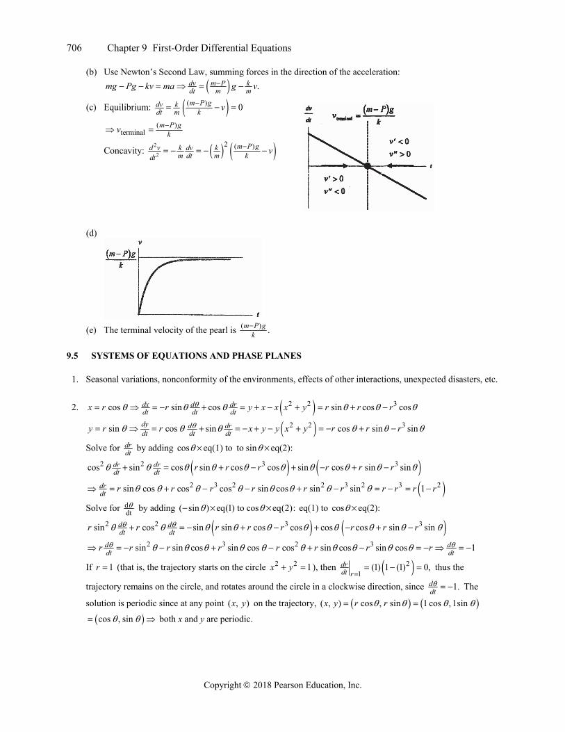
(b) Use Newton’s Second Law, summing forces in the direction of the acceleration:

.dv m P kdt m mmg Pg kv ma g v

(c) Equilibrium: ( ) 0m P gdv kdt m k v

( )terminal

m P gkv

Concavity: 2

2

2 ( )m P gd v k dv km dt m kdt

v

(d)

(e) The terminal velocity of the pearl is ( ) .m P g

k

9.5 SYSTEMS OF EQUATIONS AND PHASE PLANES

1. Seasonal variations, nonconformity of the environments, effects of other interactions, unexpected disasters, etc.

2. 2 2 3cos sin cos sin cos cosdx d drdt dt dtx r r y x x x y r r r

2 2 3sin cos sin cos sin sindy d drdt dt dty r r x y y x y r r r

Solve for drdt by adding cos eq(1) to to sin eq(2):

2 2 3 3cos sin cos sin cos cos sin cos sin sindr drdt dt r r r r r r

2 3 2 2 3 2 3 2sin cos cos cos sin cos sin sin 1drdt r r r r r r r r r r

Solve for ddt by adding ( sin ) eq(1) to cos eq(2): eq(1) to cos eq(2):

2 2 3 3sin cos sin sin cos cos cos cos sin sind ddt dtr r r r r r r r

2 3 2 3sin sin cos sin cos cos sin cos sin cos 1d ddt dtr r r r r r r r

If 1r (that is, the trajectory starts on the circle 2 2 1x y ), then 21

(1) 1 (1) 0,drdt r

thus the

trajectory remains on the circle, and rotates around the circle in a clockwise direction, since 1.ddt The

solution is periodic since at any point ( , )x y on the trajectory, ( , ) cos , sin 1 cos , 1sinx y r r

cos , sin both x and y are periodic.

Section 9.5 Systems of Equations and Phase Planes 707


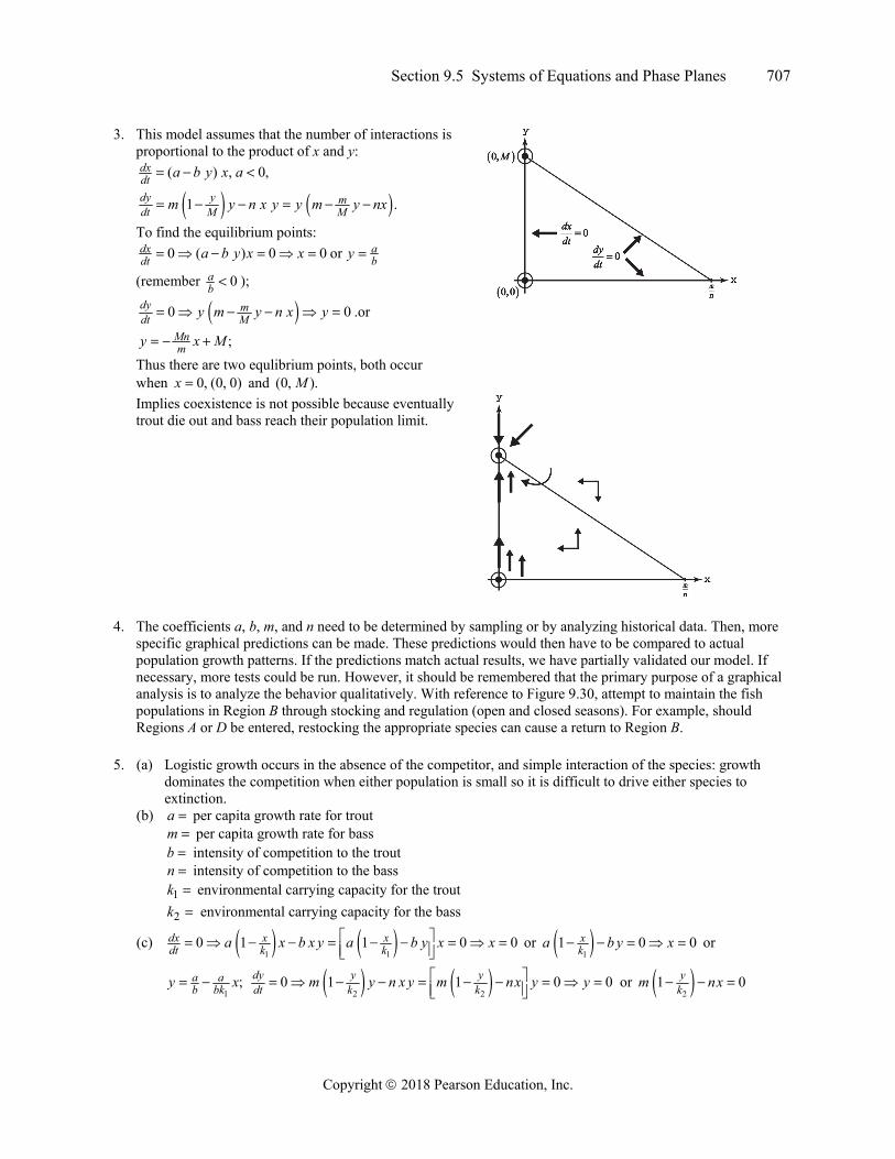
3. This model assumes that the number of interactions is proportional to the product of x and y:

( ) , 0,dxdt a b y x a

1 .dy y mdt M Mm y n x y y m y nx

To find the equilibrium points: 0 ( ) 0 0 ordx a

dt ba b y x x y

(remember 0ab );

0 0dy mdt My m y n x y .or

;Mnmy x M

Thus there are two equlibrium points, both occur when 0, (0, 0)x and (0, ).M

Implies coexistence is not possible because eventually trout die out and bass reach their population limit.

4. The coefficients a, b, m, and n need to be determined by sampling or by analyzing historical data. Then, more specific graphical predictions can be made. These predictions would then have to be compared to actual population growth patterns. If the predictions match actual results, we have partially validated our model. If necessary, more tests could be run. However, it should be remembered that the primary purpose of a graphical analysis is to analyze the behavior qualitatively. With reference to Figure 9.30, attempt to maintain the fish populations in Region B through stocking and regulation (open and closed seasons). For example, should Regions A or D be entered, restocking the appropriate species can cause a return to Region B.

5. (a) Logistic growth occurs in the absence of the competitor, and simple interaction of the species: growth dominates the competition when either population is small so it is difficult to drive either species to extinction.

(b) a per capita growth rate for trout m per capita growth rate for bass b intensity of competition to the trout n intensity of competition to the bass 1k environmental carrying capacity for the trout 2k environmental carrying capacity for the bass

(c) 1 10 1 1 0 0dx x x

dt k ka x b x y a b y x x or

11 0 0x

ka b y x or

1;a a

b bky x 2 20 1 1 0 0dy y y

dt k km y n x y m nx y y or

21 0y

km nx



0y or 22 .nk

my k x There are five cases to consider.

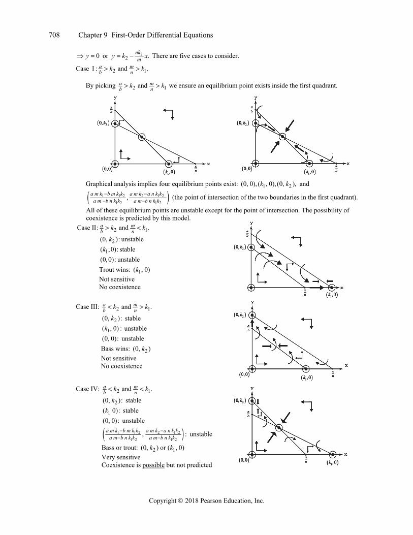
Case 2 1I : and .a mb nk k

By picking 2 1anda mb nk k we ensure an equilibrium point exists inside the first quadrant.

Graphical analysis implies four equilibrium points exist: 1 2(0, 0), ( , 0), (0, ),k k and

1 1 2 2 1 2

1 2 1 2,a m k b m k k a m k a n k k

a m b n k k a m b n k k (the point of intersection of the two boundaries in the first quadrant).

All of these equilibrium points are unstable except for the point of intersection. The possibility of coexistence is predicted by this model.

2 1Case II: and .a mb nk k

2(0, ): unstablek 1( ,0): stablek (0,0): unstable Trout wins: 1( , 0)k Not sensitive No coexistence

Case III: 2 1and .a m

b nk k

2(0, ):k stable 1( , 0) :k unstable (0, 0): unstable Bass wins: 2(0, )k Not sensitive No coexistence

Case IV: 2 1and .a m

b nk k

2(0, ):k stable 1( 0):k stable (0, 0): unstable

1 1 2 2 1 2

1 2 1 2, :a m k b m k k a m k a n k k

a m b n k k a m b n k k unstable

Bass or trout: 2 1(0, ) or ( , 0)k k Very sensitive Coexistence is possible but not predicted



If we assume 2 1anda mb nk k then graphical analysis implies four equilibrium points exist:

2 1(0, ) , ( ,0), (0, 0),k k and 1 1 2 2 1 2

1 2 1 2,a m k b m k k a m k a n k k

a m b n k k a m b n k k (the point of intersection of the two

boundaries in the first quadrant).

Case 2

12V: and (lines coincide).n ka a

b b k mk

2(0, ):k stable 1( , 0):k stable (0, 0): unstable Line segment joining 2(0, )k and 1( , 0):k stable Bass wins: 2(0, )k Not sensitive Coexistence is likely outcome Note that all points on the line segment joining 2(0, )k and 1( ,0)k are rest points.

6. For a fixed price, as Q increases, dpdt gets smaller and, possibly, becomes negative. This observation implies

that as the quantity supplied increases, the price will not rise as fast. If Q gets high enough, then the price will decrease. Next, consider :dQ

dt For a fixed quantity, as P increases, dQdt gets larger. Thus, as the market price

increases, the quantity supplied will increase at a faster rate. If P is too small, dQdt will be negative and the

quantity supplied will decrease. This observation is the traditional explanation of the effect of market price levels on the quantity supplied.

(a) 0 and 0dQdPdt dt gives the equilibrium points ( , ): (0, 0)P Q and (25.8, 775). Now 0dP

dt when

20,000PQ and 0;P 0dPdt otherwise. 0dQ

dt when 30QP and 0;Q 0dQ

dt otherwise. (b) These considerations give the following graphical analysis:

Region dPdt dQ

dt

I 0 0 II 0 0 III 0 0 IV 0 0

The equilibrium point (0, 0) is unstable. The graphical analysis for the point (25.8, 775) is inconclusive:

trajectories near the point may be periodic, or may spiral toward or away from the point. (c) The curve 0 or 20000dP

dt PQ can be thought of as the demand curve; 0 or 30dQdt Q P can be

viewed as the supply curve.



7. (a) ( )dxdt a x b x y a b y x and ( )

( )( )dydtdxdt

m nx ydy dy dy dydxdt dt dx dt dx a b y xm y nx y m nx y

(b) ( )( ) ln lnm n x ydy a m a m

dx a b y x y x y xb dy n dx b dy n dx a y b y m x nx C

ln ln ln ln ln ln ln ,a b y m n x C a b y m nx C a b y m n x Cy e x e e y e x e e y e x e e

let C a b y m nxK e y e Kx e

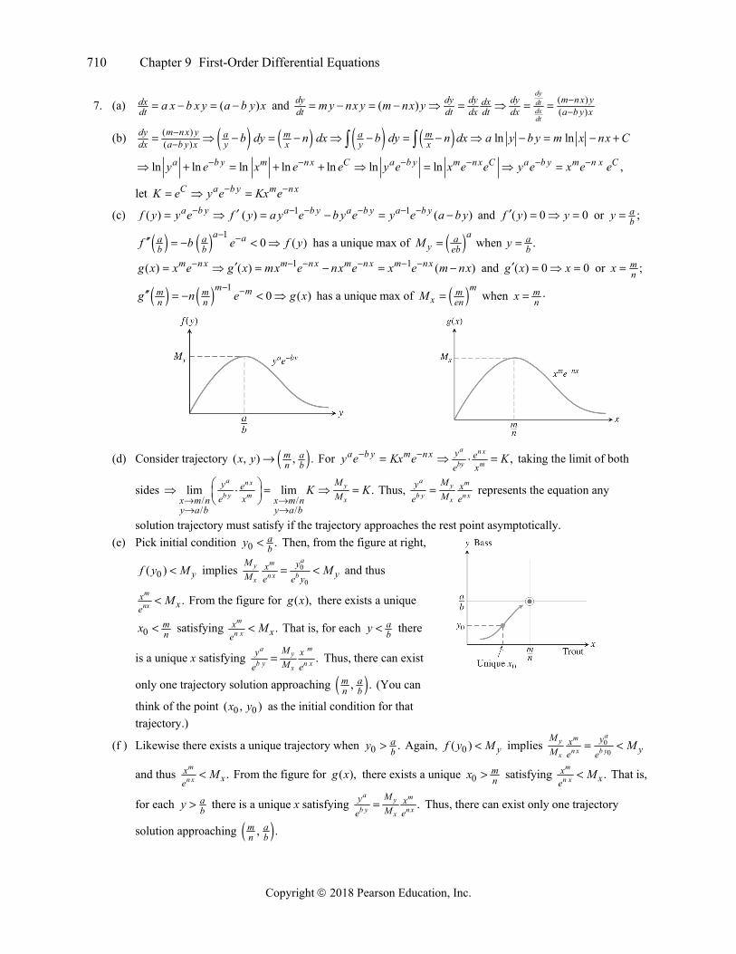
(c) 1 1( ) ( ) ( )a b y a b y a b y a b yf y y e f y a y e b y e y e a b y and ( ) 0 0f y y or ;aby

10 ( )

a aa ab bf b e f y

has a unique max of when .aa a

y eb bM y 1 1( ) ( ) ( )m nx m n x m n x m nxg x x e g x mx e nx e x e m nx and ( ) 0 0g x x or ;m

nx

10 ( )

m mm mn ng n e g x

has a unique max of mmx enM when m

nx

(d) Consider trajectory ( , ) , .m an bx y For ,

a n x

by mya b y m nx ee x

y e Kx e K taking the limit of both

sides / // /

lim lim .a n x y

b y m x

My eMe xx m n x m n

y a b y a b

K K

Thus, a my

b y n xx

My xMe e

represents the equation any

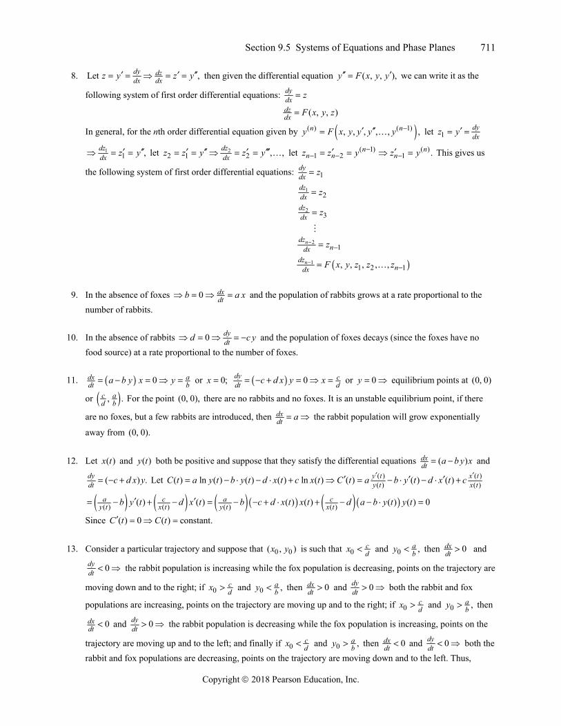
solution trajectory must satisfy if the trajectory approaches the rest point asymptotically. (e) Pick initial condition 0 .a

by Then, from the figure at right,

0( ) yf y M implies 0

0

amyn x bx

M yxyM e e y

M and thus

.m

nxx

xeM From the figure for ( ),g x there exists a unique

0mnx satisfying .

m

n xx

xeM That is, for each a

by there

is a unique x satisfying .ma

yb y n xx

M xyMe e

Thus, there can exist

only one trajectory solution approaching , .m an b (You can

think of the point 0 0( , )x y as the initial condition for that trajectory.)

(f ) Likewise there exists a unique trajectory when 0 .aby Again, 0( ) yf y M implies 0

0

amyn x b yx

M yxyM e e

M

and thus .m

n xx

xeM From the figure for ( ),g x there exists a unique 0

mnx satisfying .

m

n xx

xeM That is,

for each aby there is a unique x satisfying .

a myb y n xx

My xMe e

Thus, there can exist only one trajectory

solution approaching , .m an b



8. Let ,dy dzdx dxz y z y then given the differential equation ( , , ),y F x y y we can write it as the

following system of first order differential equations: dydx z

( , , )dzdx F x y z

In general, for the nth order differential equation given by ( ) ( 1), , , , , ,n ny F x y y y y let 1dydxz y

11 ,dz

dx z y let 22 1 2 , ,dz

dxz z y z y let ( 1) ( )1 2 1 .n n

n n nz z y z y This gives us

the following system of first order differential equations: 1dydx z

12

dzdx z

23

dzdx z

21

ndzndx z

11 2 1, , , , ,ndz

ndx F x y z z z

9. In the absence of foxes 0 dxdtb a x and the population of rabbits grows at a rate proportional to the

number of rabbits.

10. In the absence of rabbits 0 dydtd c y and the population of foxes decays (since the foxes have no

food source) at a rate proportional to the number of foxes.

11. 0dx adt ba b y x y or 0;x 0dy c

dt dc d x y x or 0y equilibrium points at (0, 0)

or , .c ad b For the point (0, 0), there are no rabbits and no foxes. It is an unstable equilibrium point, if there

are no foxes, but a few rabbits are introduced, then dxdt a the rabbit population will grow exponentially

away from (0, 0).

12. Let ( )x t and ( )y t both be positive and suppose that they satisfy the differential equations ( )dxdt a b y x and

( ) .dydt c d x y Let ( ) ( )

( ) ( )( ) ln ( ) ( ) ( ) ln ( ) ( ) ( ) ( )y t x ty t x tC t a y t b y t d x t c x t C t a b y t d x t c

( ) ( ) ( ) ( )( ) ( ) ( ) ( ) ( ) ( ) 0a c a cy t x t y t x tb y t d x t b c d x t x t d a b y t y t

Since ( ) 0 ( ) constant.C t C t

13. Consider a particular trajectory and suppose that 0 0( , )x y is such that 0cdx and 0 ,a

by then 0dxdt and

0dydt the rabbit population is increasing while the fox population is decreasing, points on the trajectory are

moving down and to the right; if 0cdx and 0 ,a

by then 0dxdt and 0dy

dt both the rabbit and fox

populations are increasing, points on the trajectory are moving up and to the right; if 0cdx and 0 ,a

by then

0dxdt and 0dy

dt the rabbit population is decreasing while the fox population is increasing, points on the

trajectory are moving up and to the left; and finally if 0cdx and 0 ,a

by then 0dxdt and 0dy

dt both the rabbit and fox populations are decreasing, points on the trajectory are moving down and to the left. Thus,



points travel around the trajectory in a counterclockwise direction. Note that we will follow the same trajectory if 0 0( , )x y starts at a different point on the trajectory.

14. There are three possible cases: If the rabbit population begins (before the wolf ) and ends (after the wolf ) at a value larger than the equilibrium level of ,c

dx then the trajectory moves closer to the equilibrium and the maximum value of the foxes is smaller. If the rabbit population begins (before the wolf ) and ends (after the wolf ) at a value smaller than the equilibrium level of ,c

dx but greater than 0, then the trajectory moves further from the equilibrium and the maximum value of the foxes is greater. If the rabbit population begins and ends very near the equilibrium value, then the trajectory will stay near the equilibrium value, since it is a stable equilibrium, and the fox population will remain roughly the same.

CHAPTER 9 PRACTICE EXERCISES

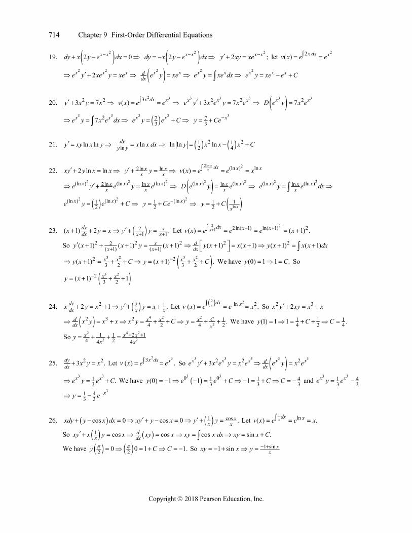
1. 3/2 3/22( 2) (3 4) 2( 2) (3 4)15 152 2 x x x xy y y yy xe x e dy x x dx e C e C

3/2 3/22( 2) (3 4) 2( 2) (3 4)15 15ln lnx x x xy C y C

2. 2 2 21

2lndyx x xyy xye e x dx y e C

3. 22

seccossec cos 0 tan cos sinx dxdy

xyx dy x y dx y x x x C

4. 22 3/2 22csc2 3 csc 0 3 2 2 2 cos 4 sinx

xx dx y x dy y dy dx y x x x x C

3/2 212 cos 2 siny x x x x C

5. ( 1) ln | |y y ye dx

xy xy ye dy y e x C

6. csc 2csc csc sin cos ( 1)x y y

yx y x xxe e e

yey xe y y y dy xe dx y y x e C

7. ( 1)( 1) 0 ( 1) ln ln( 1) ln( )dy dxy x xx x dy y dx x x dy y dx y x x C

1 1( 1) ( 1)1ln ln( 1) ln( ) ln ln ln C x C x

x xy x x C y y

8. 11

2

ln 1 12 1 21 12 1 11

1 ln ln 2ln lnyydy y ydx

x y yyy y x x C x C C x

9. /2 /212 22 .x xxy y xe y y e

12 /21

2( ) , ( ) .dx xP x v x e e

2 2/2 /2 /2 /2 /2 /2 /212 2 2 2 4 4

x x x x x x xx x d x x xdxe y e y e e e y e y C y e C

Chapter 9 Practice Exercises 713


10. 2 sin 2 2 sin .y x xy e x y y e x 2 2( ) 2, ( ) .dx xP x v x e e

2 2 2 2 22 2 sin 2 sin 2 sin sin cosx x x x x x x x xddxe y e y e e x e x e y e x e y e x x C

2sin cosx xy e x x Ce

11. 21 2 1 12 1 .x x x

xy y x y y

22 2ln ln 2( ) .dxx x xv x e e e x

2

22 2 2 1 1

2 22 1 1d x Cdx x x

x y xy x x y x x y x C y

12. 12 ln 2ln .xxy y x x y y x

ln 1( ) .dxx x

xv x e e

2 2 21 1 2 1 2 1ln ln ln lndx x x dx x x xy y x y x y x C y x x Cx

13. 1 11 0 1 .

x x

x xx x x x x x e e

e ee dy ye e dx e y e y e y y

1ln 1

( ) 1.xe dx x

xee xv x e e e

1 11 1 1 1 1

x x

x xx x x x x x xe e d

dxe ee y e y e e y e e y e C

1 1

x x

x xe C e Ce e

y

14. 4 0 4 ( ) 1,dyx x xdxe dy e y x dx y xe p x 1 2( ) 4dx dyx x x x

dxv x e e e ye x e

2 2 2 24 4 2 2x x x x x x x x x xddx y e x e y e x e dx y e xe e C y xe e Ce

15. 2 2 2 33 0 3 3ddxx y dy y dx x dy y dx y dy xy y dy xy y C

16. 2 333 cos 0 cos .xx dy y x x dx y y x x Let 3 33ln ln 3( ) .

dxx x xv y e e e x

Then 3 23 cosx y x y x and 3 cos sin .x y x dx x C So 3 siny x x C

17. 23 2 3

cossin cos sin dy

yy x y x dx 2 2sec sin (1 cos ) y dy x x dx

313tan cos cosy x x C

18. 4 ( ) 0x dy x y dx 4 ( ) x dy x y dx 3 yxy x 31 ;xy y x

1 ln( ) x dx xv x e e x 4xy y x 4( )d

dx xy x 4 515 xy x dx x C 41

5Cxy x



19. 22 0x xdy x y e dx 2

2 x xdy x y e dx 2

2 ;x xy xy xe let 22 ( ) x dx xv x e e

2 22x x xe y xe y xe 2x xd

dx e y xe 2x xe y xe dx

2x x xe y xe e C

20. 2 23 7y x y x 2 33( ) x dx xv x e e

3 3 32 23 7x x xe y x e y x e 3 327x xD e y x e

3 327x xe y x e dx 3 373

x xe y e C 37

3xy Ce

21. ln lny xy x y ln ln dyy y x x dx 2 21 1

2 4ln ln lny x x x C

22. 2 ln lnxy y x x 2ln lnx xx xy y

2ln 2 (ln ) ln( )x

x dx x xv x e e x 2 2 2(ln ) (ln ) (ln )2ln lnx x xx x

x xe y e y e 2 2(ln ) (ln )lnx xxxD e y e

2 2(ln ) (ln )lnx xxxe y e dx

2 2(ln ) (ln )12

x xe y e C 2(ln )1

2xy Ce ln

1 12 xx

y C

23. 21 1( 1) 2 .dy x

dx x xx y x y y Let

2 21 2ln( 1) ln( 1) 2( ) ( 1) .x dx x xv x e e e x

So 2 2 2 2 22( 1) ( 1)( 1) ( 1) ( 1) ( 1) ( 1) ( 1) ( 1)x dx x dxy x x y x y x x x y x x x dx

3 2 3 22 23 2 3 2( 1) ( 1) .x x x xy x C y x C We have (0) 1 1 .y C So

3 223 2( 1) 1x xy x

24. 2 2 12 1 .dydx x xx y x y y x Let 2 2ln 2( ) .x dx xv x e e x So 2 32x y xy x x

4 2 2

22 3 2 1

4 2 4 2 .d x x x Cdx x

x y x x x y C y We have 1 1 14 2 4(1) 1 1 .y C C

2 4 2

2 22 11 1

4 24 4So x x x

x xy

25. 2 23 .dydx x y x Let

2 33( ) .x dx xv x e e So 3 3 3 3 32 2 23x x x x xddxe y x e y x e e y x e

3 313 .x xe y e C We have

3 30 01 1 43 3 3(0) 1 1 1y e e C C C and

3 31 43 3

x xe y e 31 4

3 3xy e

26. cos1cos 0 cos 0 .xx xxdy y x dx xy y x y y Let

1 ln( ) .x dx xv x e e x

So 1 cos cos cos sin .dx dxxy x y x xy x xy x dx xy x C

We have 2 20 0 1 1.y C C So 1 sin1 sin xxxy x y



27. 3 22( 2) 3 3 .x xxxxy x y x e y y x e Let 2

22ln( ) .

x xx dx x x e

xv x e e

So 2 2 2 22 3 3 3 .

x x x xe e x d e ex dxx x x x

y y y y x C We have (1) 0 0 3(1) 3y C C

223 3 (3 3)

x xex

y x y x e x

28. 3 2 3 32 23 2 0 0 1 .x xydx dx x dxdy y dy y y dy y yy dx x xy dy x x

3ln 33( ) 1 ( ) 3ln ( ) y y yyP y P y dy y y v y e y e

3 3 2 3 2 23 1 2 2 2 2 2y y y y y yyy e x y e x y e y e x y e dy e y y C

22 2 23 .yy y Ce

xy

We have 12(1 2 2)

2(2) 1 1 4Cey C e and

2 12 2 2 43yy y e

xy

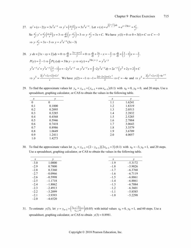
29. To find the approximate values let 1 1 1cos (0.1)n n n ny y y x with 0 00, 0,x y and 20 steps. Use a spreadsheet, graphing calculator, or CAS to obtain the values in the following table.

x y 0 0 0.1 0.1000 0.2 0.2095 0.3 0.3285 0.4 0.4568 0.5 0.5946 0.6 0.7418 0.7 0.8986 0.8 1.0649 0.9 1.2411 1.0 1.4273

x y 1.1 1.6241 1.2 1.8319 1.3 2.0513 1.4 2.2832 1.5 2.5285 1.6 2.7884 1.7 3.0643 1.8 3.3579 1.9 3.6709 2.0 4.0057

30. To find the approximate values let 1 1 12 2 3 (0.1)n n n ny y y x with 0 03, 1,x y and 20 steps. Use a spreadsheet, graphing calculator, or CAS to obtain the values in the following table.

x y –3.0 1.0000 –2.9 0.7000 –2.8 0.3360 –2.7 –0.0966 –2.6 –0.5998 –2.5 –1.1718 –2.4 –1.8062 –2.3 –2.4913 –2.2 –3.2099 –2.1 –3.9393 –2.0 –4.6520

x y –1.9 –5.3172 –1.8 –5.9026 –1.7 –6.3768 –1.6 –6.7119 –1.5 –6.8861 –1.4 –6.8861 –1.3 –6.7084 –1.2 –6.3601 –1.1 –5.8585 –1.0 –5.2298

31. To estimate (3),y let 1 1

1

21 1 (0.05)n n

n

x yn xy y

with initial values 0 00, 1,x y and 60 steps. Use a

spreadsheet, graphing calculator, or CAS to obtain (3) 0.8981.y



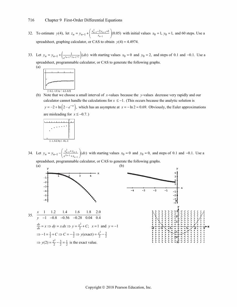
32. To estimate (4),y let 2

1 1

1

2 11 (0.05)n n

n

x yn n xz y

with initial values 0 01, 1,x y and 60 steps. Use a

spreadsheet, graphing calculator, or CAS to obtain (4) 4.4974.y

33. Let 21 11

1 ( )x yn nn n ey y dx with starting values 0 0x and 0 2,y and steps of 0.1 and 0.1. Use a

spreadsheet, programmable calculator, or CAS to generate the following graphs. (a)

(b) Note that we choose a small interval of -valuesx because the -valuesy decrease very rapidly and our

calculator cannot handle the calculations for x 1. (This occurs because the analytic solution is

2 ln 2 ,xy e which has an asymptote at ln 2 0.69.x Obviously, the Euler approximations

are misleading for 0.7.x )

34. Let 2

1 11

11 ( )n n

ynn

x yn n e x

y y dx

with starting values 0 0x and 0 0,y and steps of 0.1 and 0.1. Use a

spreadsheet, programmable calculator, or CAS to generate the following graphs. (a)

(b)

35. 1 1.2 1.4 1.6 1.8 2.01 0.8 0.56 0.28 0.04 0.4

xy

2

2 ;dy xdx x dy x dx y C 1x and 1y

23 312 2 2 21 (exact) xC C y

2 32 12 2 2(2)y is the exact value.



36. 1 1.2 1.4 1.6 1.8 2.01 0.8 0.6333 0.4904 0.3654 0.2544

xy

1 1 ln | | ;dydx x xdy dx y x C 1x and 1y

1 ln1 1 (exact) ln | | 1C C y x (2) ln 2 1 0.3069y is the exact value.

37. 1 1.2 1.4 1.6 1.8 2.01 1.2 0.488 1.9046 2.5141 3.4192

xy

2

2lndy dy xdx yxy x dx y C

2 2 22 2 21 ;

x x xC Cy e e e C e 1x and 1y 221/2 1/2 1/2

1 11 (exact)x

C e C e y e e

2 1 /2 3/2(2) 4.4817x

e y e

is the exact value.

38. 1 1.2 1.4 1.6 1.8 2.01 1.2 1.3667 1.5130 1.6452 1.7688

xy

21 ;dy ydx y yy dy dx x C 1x and 1y

21 12 21 2 1C C y x

(exact) 2 1 (2) 3 1.7321y x y is the exact value.

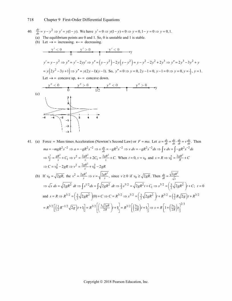
39. 2 1 ( 1)( 1).dydx y y y y We have 0 ( 1) 0, ( 1) 0 1, 1.y y y y

(a) Equilibrium points are 1 (stable) and 1 (unstable) (b) 2 21 2 2 1 2 ( 1)( 1).y y y yy y y y y y y So 0 0, 1, 1.y y y y

(c)



40. 2 (1 ).dydx y y y y y We have 0 (1 ) 0 0, 1 0 0, 1.y y y y y y

(a) The equilibrium points are 0 and 1. So, 0 is unstable and 1 is stable. (b) Let increasing. decreasing.

2 2 2 2 2 3 3 22 2 2 2 2 3y y y y y yy y y y y y y y y y y y y y y

22 3 1 (2 1)( 1).y y y y y y y So, 120 0, 2 1 0, 1 0 0, , 1.y y y y y y y

Let concave up, concave down.

(c)

41. (a) Force Mass times Acceleration (Newton’s Second Law) or .F ma Let .dv dv ds dvdt ds dt dsa v Then

2 2 2 2 2 2 2 2 2 2dvdsma mgR s a gR s v gR s v dv gR s ds v dv gR s ds

2 2 22 2 221 12 2 .gR gR gRv

s s sC v C C When 00,t v v and 222

0gRRs R v C

222 2 20 02 2gR

sC v gR v v gR

(b) If 0 2 ,v gR the 2 22 22 ,gR gR

s sv v since 0v if 0 2 .v gR Then 22gRds

dt s

2 1/2 2 3/2 2 3/2 23213 22 2 2 2 ;s ds gR dt s ds gR dt s gR t C s gR t C

0t

and 3/2 2 3/2 3/2 2 3/2 3/23 3 32 2 22 (0) 2 2s R R gR C C R s gR t R R g t R

0 02/33 2 3 33/2 1/2 3/2 3/23

2 2 2 22 1 1 1 1gR v vR R RR R g t R t R t s R t



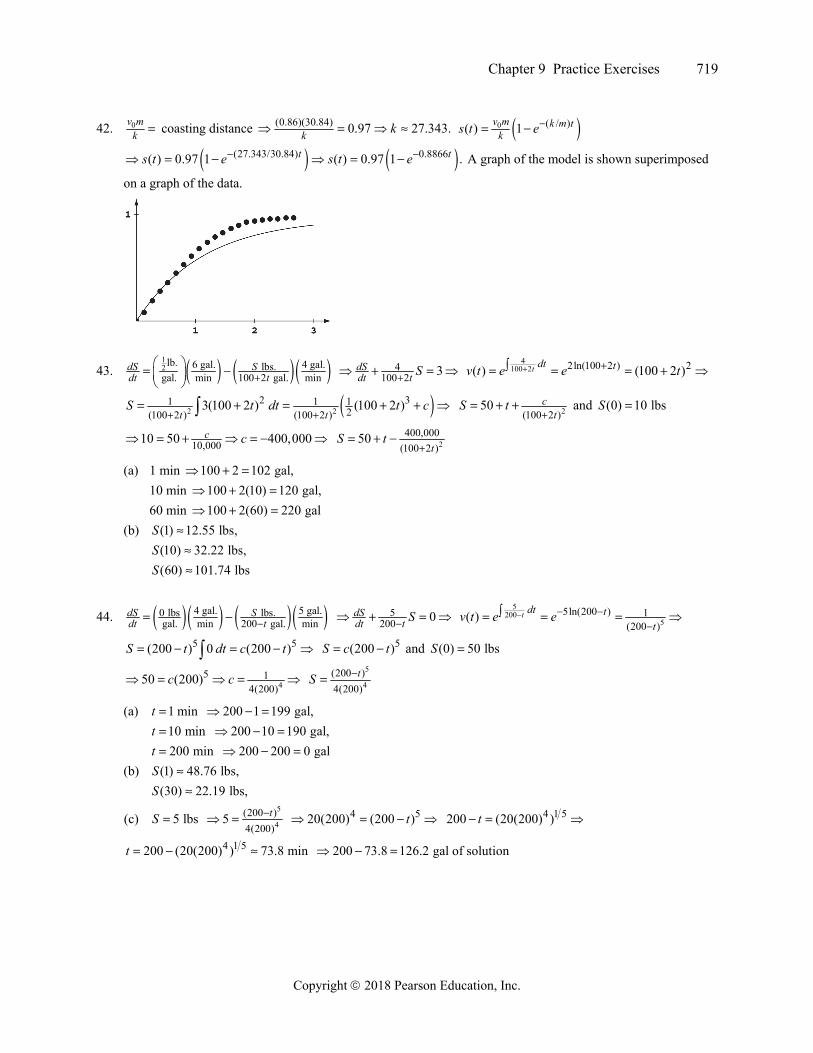
42. 0v mk coasting distance (0.86)(30.84) 0.97 27.343.k k 0 ( / )( ) 1v m k m t

ks t e

(27.343/30.84) 0.8866( ) 0.97 1 ( ) 0.97 1 .t ts t e s t e A graph of the model is shown superimposed

on a graph of the data.

43. 12 lb. 6 gal. 4 gal. lbs.gal. min 100 2 gal. min

dS Sdt t

4100 2 3dS

dt t S 4

100 2 2ln(100 2 ) 2( ) (100 2 )t dt tv t e e t

2 22 31 1 1

2(100 2 ) (100 2 )3(100 2 ) (100 2 )

t tS t dt t c

2(100 2 )

50 ct

S t

and (0) 10 lbsS

10,00010 50 400,000c c 2400,000

(100 2 )50

tS t

(a) 1 min 100 2 102 gal, 10 min 100 2(10) 120 gal, 60 min 100 2(60) 220 gal

(b) (1) 12.55 lbs,S (10) 32.22 lbs,S (60) 101.74 lbsS

44. 4 gal. 5 gal.0 lbs lbs.gal. min 200 gal. min

dS Sdt t 5

200 0dSdt t S

5200

5 5ln(200 ) 1

(200 )( ) t dt t

tv t e e

5 5(200 ) 0 (200 )S t dt c t 5(200 )S c t and (0) 50 lbsS

45 1

4(200)50 (200)c c

5

4(200 )4(200)

tS

(a) 1 mint 200 1 199 gal, 10 mint 200 10 190 gal, 200 mint 200 200 0 gal

(b) (1) 48.76 lbs,S (30) 22.19 lbs,S

(c) 5 lbsS 5

4(200 )4(200)

5 t 4 520(200) (200 )t 4 1 5200 (20(200) )t

4 1 5200 (20(200) ) 73.8 mint 200 73.8 126.2 gal of solution



CHAPTER 9 ADDITIONAL AND ADVANCED EXERCISES

1. (a) 1lndy dy dyA A A A Adt V V y c V y c V Vk c y dy k y c dt k dt k dt y c k t C

1 .AVk tCy c e e Apply the initial condition, 0 0 0(0)y y y c C C y c

0 .AVk ty c y c e

(b) Steady state solution: 0 0lim ( ) lim (0)AVk t

tty y t c y c e c y c c

2. .d mv d mvdm dm dv dm dm dm dv dmdt dt dt dt dt dt dt dt dt dtF v u F v u F m v v u F m u

.dmdt b m b t C At 00, ,t m m so 0C m and 0 .m m b t

Thus 0

000 0 1lnu b m b tdv dv

dt dt mm b tF m b t u b m b t g g v gt u C

0v at 10 0.t C So 0 0

0 0ln lnm b t m b tdy

m dt mv gt u y gt u dt and , 0u c y at

0 0

0

2120 lnm b t m b t

mbt y gt c t

3. (a) Let y be any function such that ( ) ( ) ( ) ,v x y v x Q x dx C ( )( ) .P x dxv x e Then

( ) ( ) ( ) ( ) ( ).ddx v x y v x y y v x v x Q x We have ( )( ) P x dxv x e

( )( ) ( ) ( ) ( ).P x dxv x e P x v x P x Thus ( ) ( ) ( ) ( ) ( ) ( ) ( )v x y y v x P x v x Q x y yP x Q x the given y is a solution.

(b) If v and Q are continuous on [ , ]a b and ( , ),x a b then 0

( ) ( ) ( ) ( )xd

dx xv t Q t dt v x Q x

0( ) ( ) ( ) ( ) .

xx

v t Q t dt v x Q x dx So 0 0 ( ) ( ) .C y v x v x Q x dx From part (a),

( ) ( ) ( ) .v x y v x Q x dx C Substituting for C: 0 0( ) ( ) ( ) ( ) ( ) ( )v x y v x Q x dx y v x v x Q x dx

0 0( )v x y y v x when 0.x x

4. (a) 0( ) 0, ( ) 0.y P x y y x Use ( )( ) P x dxv x e as an integrating factor. Then ( ) 0ddx v x y

( )( ) P x dxv x y C y Ce and ( )1 1 ,P x dxy C e ( )

2 2 ,P x dxy C e 1 0 2 0 0,y x y x

( ) ( )1 2 1 2 3

P x dx P x dxy y C C e C e and 1 2 0 0 0.y y So 1 2y y is a solution to

( ) 0y P x y with 0 0.y x

(b) ( ) ( )1 2 1 2 1 2 3( ) ( ) ( ) 0.P x dx P x dxd d d d

dx dx dx dxv x y x y x e e C C C C C

1 2 1 2( ) ( ) ( ) ( ) ( ) ( ) 0ddx v x y x y x dx v x y x y x dx C

(c) ( )1 1 ,P x dxy C e ( )

2 2 ,P x dxy C e 1 2.y y y So ( ) ( )0 1 20 0P x dx P x dxy x C e C e

1 2 1 2 1 20 ( ) ( )C C C C y x y x for .a x b

Chapter 9 Additional and Advanced Exercises 721


5. 2 2

2 2 1 1/ ( )0 ( ) 0

x ydy y y yx dx dvdx xy y x y x x x v x v F vx y dx x ydy F F v v

21

22142 1

0 ln ln 2 1 4ln ln 2 1v

vdv ydx dv dxx x xvv v

C x v C x C

2 2

224 2 2 2 2 2 2 2 2 2ln ln ln 2 2 2y x C

xx C x y x C x y x e x y x C

6. 2

2 2

22 2 20 ( ) 0y x ydy dy y y y dx dv

dx dx x x x xx v v vx dy y x y dx F F v v v

21 1

/ln ln lndx dv xx v y x yv

C x C x C x C

7. // /0 ( ) 0

y x

vxe ydy y yy x y x v dx dv

dx x x x x v e vxe y dx xdy e F F v e v

/ln lnvv y xdx dv

x eC x e C x e C

8.

211

1 111 11

0 ( ) 0 0yx

y vvx

x y v dvdy y v dx dv dxdx x y x v x x vv

x y dy x y dx F F v

2 2

21 2 1121 1

0 ln tan ln 1 2ln 2 tan ln 1vdv ydx dvx xv v

x v v C x v C

2 2

22 1 1 2 2ln 2 tan ln 2 tan lny y x y

x xxx C y x C

9. cos 1cos cos 1 ( ) cos 1 0y y x y y y dx dv

x x x x x x v v vy F F v v v

sec 1 0 ln ln sec 1 tan 1 ln ln sec 1 tan 1y ydxx x xv dv x v v C x C

10. sin cos

cossin cos cos 0 tan ( ) tan

y yx x

yx

x yy y y dy y y yx x x dx x x xx

x y dx x dy F F v v v

tan 0 cot 0 ln ln sin ln ln sin ydx dv dxx x xv v v

v dv x v C x C

Documents

CHAPTER 9 FIRST-ORDER DIFFERENTIAL EQUATIONS · the following system of first order differential equations: 1 dy dx z 1 2 dz dx z 2 3 dz dx z 2 1 dzn dx zn 1 ,, , , ,12 1 dzn dx Fxyz