Embed Size (px)
Citation preview
chapter five
Device characterization
Raja Balasubramanian
Xerox Solutions & Services Technology Center
Contents
5.1 Introduction 5.2 Basic concepts
5.2.1 Device calibration5.2.2 Device characterization5.2.3 Input device calibration and characterization5.2.4 Output device calibration and characterization
5.3 Characterization targets and measurement techniques 5.3.1 Color target design 5.3.2 Color measurement techniques
5.3.2.1 Visual approaches5.3.2.2 Instrument-based approaches
5.3.3 Absolute and relative colorimetry5.4 Multidimensional data fitting and interpolation
5.4.1 Linear least-squares regression5.4.2 Weighted least-squares regression 5.4.3 Polynomial regression5.4.4 Distance-weighted techniques
5.4.4.1 Shepard’s interpolation5.4.4.2 Local linear regression
5.4.5 Lattice-based interpolation5.4.6 Sequential interpolation5.4.7 Neural networks5.4.8 Spline fitting
5.5 Metrics for evaluating device characterization
-ColorBook Page 269 Wednesday, November 13, 2002 10:55 AM
© 2003 by CRC Press LLC
270 Digital Color Imaging Handbook
5.6 Scanners5.6.1 Calibration5.6.2 Model-based characterization 5.6.3 Empirical characterization
5.7 Digital still cameras5.7.1 Calibration5.7.2 Model-based characterization5.7.3 Empirical characterization5.7.4 White-point estimation and chromatic adaptation
transform 5.8 CRT displays
5.8.1 Calibration5.8.2 Characterization5.8.3 Visual techniques
5.9 Liquid crystal displays5.9.1 Calibration5.9.2 Characterization
5.10 Printers5.10.1 Calibration
5.10.1.1 Channel-independent calibration 5.10.1.2 Gray-balanced calibration
5.10.2 Model-based printer characterization5.10.2.1 Beer–Bouguer model5.10.2.2 Kubelka–Munk model5.10.2.3 Neugebauer model
5.10.3 Empirical techniques for forward characterization5.10.3.1 Lattice-based techniques 5.10.3.2 Sequential interpolation 5.10.3.3 Other empirical approaches
5.10.4 Hybrid approaches5.10.5 Deriving the inverse characterization function
5.10.5.1 CMY printers5.10.5.2 CMYK printers
5.10.6 Scanner-based printer characterization 5.10.7 Hi-fidelity color printing
5.10.7.1 Forward characterization5.10.7.2 Inverse characterization
5.10.8 Projection transparency printing5.11 Characterization for multispectral imaging5.12 Device emulation and proofing5.13 Commercial packages5.14 ConclusionsAcknowledgmentReferencesAppendix 5.AAppendix 5.B
-ColorBook Page 270 Wednesday, November 13, 2002 10:55 AM
© 2003 by CRC Press LLC
Chapter five: Device characterization 271
5.1 Introduction
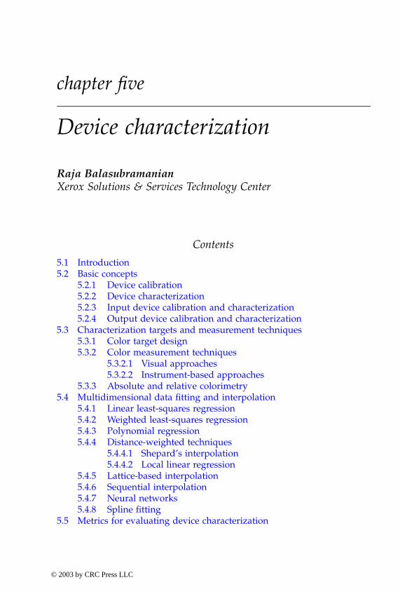
Achieving consistent and high-quality color reproduction in a color imagingsystem necessitates a comprehensive understanding of the color character-istics of the various devices in the system. This understanding is achievedthrough a process of device characterization. One approach for doing this isknown as closed-loop characterization, where a specific input device is opti-mized for rendering images to a specific output device. A common exampleof closed-loop systems is found in offset press printing, where a drum scan-ner is often tuned to output CMYK signals for optimum reproduction on aparticular offset press. The tuning is often carried out manually by skilledpress operators. Another example of a closed-loop system is traditionalphotography, where the characteristics of the photographic dyes, film, devel-opment, and printing processes are co-optimized (again, often manually) forproper reproduction. While the closed-loop paradigm works well in theaforementioned examples, it is not an efficient means of managing color inopen digital color imaging systems where color can be exchanged among alarge and variable number of color devices. For example, a system compris-ing three scanners and four printers would require closed-looptransformations. Clearly, as more devices are added to the system, it becomesdifficult to derive and maintain characterizations for all the various combi-nations of devices.
An alternative approach that is increasingly embraced by the digitalcolor imaging community is the device-independent paradigm, where trans-lations among different device color representations are accomplished viaan intermediary device-independent color representation. This approach ismore efficient and easily managed than the closed-loop model. Taking thesame example of three scanners and four printers now requires only 3 + 4= 7 transformations. The device-independent color space is usually basedon a colorimetric standard such as CIE XYZ or CIELAB. Hence, the visualsystem is explicitly introduced into the color imaging path. The closed-loopand device-independent approaches are compared in Figure 5.1.
The characterization techniques discussed in this chapter subscribe tothe device-independent paradigm and, as such, involve deriving transfor-mations between device-dependent and colorimetric representations.Indeed, a plethora of device characterization techniques have been reportedin the literature. The optimal approach depends on several factors, includingthe physical color characteristics of the device, the desired quality of thecharacterization, and the cost and effort that one is willing to bear to performthe characterization. There are, however, some fundamental concepts thatare common to all these approaches. We begin this chapter with a descriptionof these concepts and then provide a more detailed exposition of character-ization techniques for commonly encountered input and output devices. Tokeep the chapter to a manageable size, an exhaustive treatment is given toonly a few topics. The chapter is complemented by an extensive set ofreferences for a more in-depth study of the remaining topics.
3 4× 12=
-ColorBook Page 271 Wednesday, November 13, 2002 10:55 AM
© 2003 by CRC Press LLC
272 Digital Color Imaging Handbook
5.2 Basic concepts
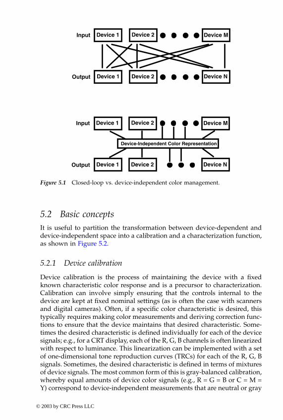
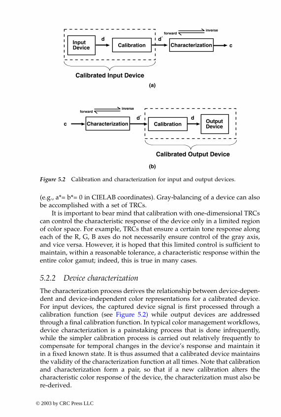
It is useful to partition the transformation between device-dependent anddevice-independent space into a calibration and a characterization function,as shown in Figure 5.2.
5.2.1 Device calibration
Device calibration is the process of maintaining the device with a fixedknown characteristic color response and is a precursor to characterization.Calibration can involve simply ensuring that the controls internal to thedevice are kept at fixed nominal settings (as is often the case with scannersand digital cameras). Often, if a specific color characteristic is desired, thistypically requires making color measurements and deriving correction func-tions to ensure that the device maintains that desired characteristic. Some-times the desired characteristic is defined individually for each of the devicesignals; e.g., for a CRT display, each of the R, G, B channels is often linearizedwith respect to luminance. This linearization can be implemented with a setof one-dimensional tone reproduction curves (TRCs) for each of the R, G, Bsignals. Sometimes, the desired characteristic is defined in terms of mixturesof device signals. The most common form of this is gray-balanced calibration,whereby equal amounts of device color signals (e.g., R = G = B or C = M =Y) correspond to device-independent measurements that are neutral or gray
Device-Independent Color Representation
Input
Output
Device 1 Device 2
Device 2Device 1
Device M
Device N
Input
Output
Device 1 Device 2
Device 2Device 1
Device M
Device N
Figure 5.1 Closed-loop vs. device-independent color management.
-ColorBook Page 272 Wednesday, November 13, 2002 10:55 AM
© 2003 by CRC Press LLC
Chapter five: Device characterization 273
(e.g., a*= b*= 0 in CIELAB coordinates). Gray-balancing of a device can alsobe accomplished with a set of TRCs.
It is important to bear mind that calibration with one-dimensional TRCscan control the characteristic response of the device only in a limited regionof color space. For example, TRCs that ensure a certain tone response alongeach of the R, G, B axes do not necessarily ensure control of the gray axis,and vice versa. However, it is hoped that this limited control is sufficient tomaintain, within a reasonable tolerance, a characteristic response within theentire color gamut; indeed, this is true in many cases.
5.2.2 Device characterization
The characterization process derives the relationship between device-depen-dent and device-independent color representations for a calibrated device.For input devices, the captured device signal is first processed through acalibration function (see
Figure 5.2) while output devices are addressedthrough a final calibration function. In typical color management workflows,device characterization is a painstaking process that is done infrequently,while the simpler calibration process is carried out relatively frequently tocompensate for temporal changes in the device’s response and maintain itin a fixed known state. It is thus assumed that a calibrated device maintainsthe validity of the characterization function at all times. Note that calibrationand characterization form a pair, so that if a new calibration alters thecharacteristic color response of the device, the characterization must also bere-derived.
InputDevice Calibration Characterization
d d `c
forwardinverse
Calibrated Input Device
dd `
Calibrated Output Device
OutputDeviceCalibrationc
forwardinverse
Characterization
(a)
(b)
Figure 5.2 Calibration and characterization for input and output devices.
-ColorBook Page 273 Wednesday, November 13, 2002 10:55 AM
© 2003 by CRC Press LLC
274 Digital Color Imaging Handbook
The characterization function can be defined in two directions. The for-ward characterization transform defines the response of the device to aknown input, thus describing the color characteristics of the device. Theinverse characterization transform compensates for these characteristics anddetermines the input to the device that is required to obtain a desiredresponse. The inverse function is used in the final imaging path to performcolor correction to images.
The sense of the forward function is different for input and outputdevices. For input devices, the forward function is a mapping from a device-independent color stimulus to the resulting device signals recorded whenthe device is exposed to that stimulus. For output devices, this is a mappingfrom device-dependent colors driving the device to the resulting renderedcolor, in device-independent coordinates. In either case, the sense of theinverse function is the opposite to that of the forward function.
There are two approaches to deriving the forward characterization func-tion. One approach uses a model that describes the physical process by whichthe device captures or renders color. The parameters of the model are usuallyderived with a relatively small number of color samples. The secondapproach is empirical, using a relatively large set of color samples in con-junction with some type of mathematical fitting or interpolation techniqueto derive the characterization function. Derivation of the inverse functioncalls for an empirical or mathematical technique for inverting the forwardfunction. (Note that the inversion does not require additional color samples;it is purely a computational step.)
A primary advantage to model-based approaches is that they requirefewer measurements and are thus less laborious and time consuming thanempirical methods. To some extent, a physical model can be generalized fordifferent image capture or rendering conditions, whereas an empirical tech-nique is typically optimized for a restrictive set of conditions and must be re-derived as the conditions change. Model-based approaches generate relativelysmooth characterization functions, whereas empirical techniques are subjectto additional noise from measurements and often require additional smooth-ing on the data. However, the quality of a model-based characterization isdetermined by the extent to which the model reflects the real behavior of thedevice. Certain types of devices are not readily amenable to tractable physicalmodels; thus, one must resort to empirical approaches in these cases. Also,most model-based approaches require access to the raw device, while empir-ical techniques can often be applied in addition to simple calibration andcharacterization functions already built into the device. Finally, hybrid tech-niques can be employed that borrow strengths from both model-based andempirical approaches. Examples of these will be presented later in the chapter.
The output of the calibration and characterization process is a set ofmappings between device-independent and -dependent color descriptions;these are usually implemented as some combination of power-law mapping,3
×
3 matrix conversion, white-point normalization, and one-dimensionaland multidimensional lookup tables. This information can be stored in a
-ColorBook Page 274 Wednesday, November 13, 2002 10:55 AM
© 2003 by CRC Press LLC
Chapter five: Device characterization 275
variety of formats, of which the most widely adopted industry standard isthe International Color Consortium (ICC) profile (www.color.org). For print-ers, the Adobe Postscript language (Level 2 and higher) also contains oper-ators for storing characterization information.
1
It is important to bear in mind that device calibration and characteriza-tion, as described in this chapter, are functions that depend on color signalsalone and are not functions of time or the spatial location of the captured orrendered image. The overall accuracy of a characterization is thus limitedby the ability of the device to exhibit spatial uniformity and temporal sta-bility. Indeed, in reality, the color characteristics of any device will vary tosome degree over its spatial footprint and over time. It is generally goodpractice to gather an understanding of these variances prior to or during thecharacterization process. This may be accomplished by exercising the deviceresponse with multiple sets of stimuli in different spatial orientations andover a period of time. The variation in the device’s response to the samestimulus across time and space is then observed. A simple way to reducethe effects of nonuniformity and instability during the characterization pro-cess is to average the data at different points in space and time that corre-spond to the same input stimulus.
Another caution to keep in mind is that many devices have color-cor-rection algorithms already built into them. This is particularly true of low-cost devices targeted for consumers. These algorithms are based in part oncalibration and characterization done by the device manufacturer. In somedevices, particularly digital cameras, the algorithms use spatial context andimage-dependent information to perform the correction. As indicated in thepreceding paragraph, calibration or characterization by the user is best per-formed if these built-in algorithms can be deactivated or are known to theextent that they can be inverted. (This is especially true of the model-basedapproaches.) Reverse engineering of built-in correction functions is notalways an easy task. One can also argue that, in many instances, the built-in algorithms provide satisfactory quality for the intended market, hence notrequiring additional correction. Device calibration and characterization istherefore recommended only when it is necessary and possible to fullycontrol the color characteristics of the device.
5.2.3 Input device calibration and characterization
There are two main types of digital color input devices: scanners, whichcapture light reflected from or transmitted through a medium, and digitalcameras, which directly capture light from a scene. The captured light passesthrough a set of color filters (most commonly, red, green, blue) and is thensensed by an array of charge-coupled devices (CCDs). The basic model thatdescribes the response of an image capture device with
M
filters is given by
(5.1)Di S λ( )λεV∫ qi λ( )u λ( )∂λ ni+= ,i 1,…,M=
-ColorBook Page 275 Wednesday, November 13, 2002 10:55 AM
© 2003 by CRC Press LLC
276 Digital Color Imaging Handbook
where
D
i
= sensor response
S(
λ
)
= input spectral radiance
q
i
(
λ
)
= spectral sensitivity of the
i
th sensor
u(
λ
)
= detector sensitivity
n
i
= measurement noise in the
i
th channel
V
= spectral regime outside which the device sensitivity is negligible
Digital still cameras often include an infrared (IR) filter; this would be incor-porated into the
u(
λ
)
term. Invariably,
M
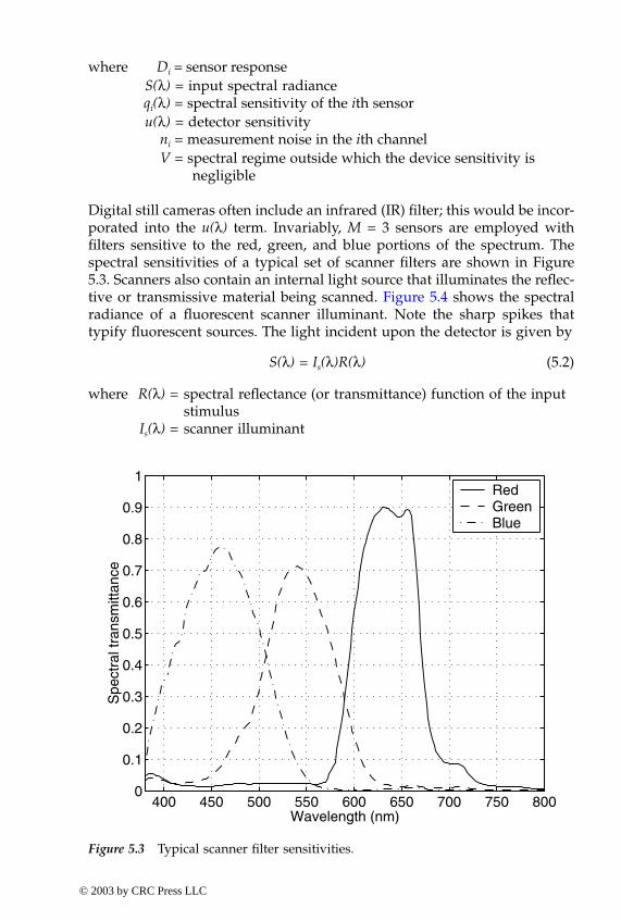
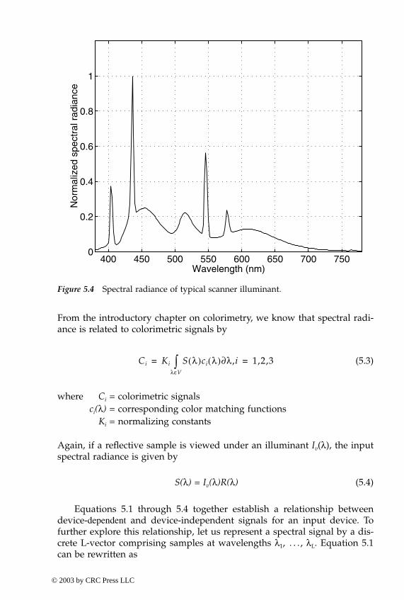
= 3 sensors are employed withfilters sensitive to the red, green, and blue portions of the spectrum. Thespectral sensitivities of a typical set of scanner filters are shown in Figure5.3. Scanners also contain an internal light source that illuminates the reflec-tive or transmissive material being scanned. Figure 5.4 shows the spectralradiance of a fluorescent scanner illuminant. Note the sharp spikes thattypify fluorescent sources. The light incident upon the detector is given by
S(
λ
) = I
s
(
λ
)R(
λ
)
(5.2)
where
R(
λ
)
= spectral reflectance (or transmittance) function of the input stimulus
I
s
(
λ
)
= scanner illuminant
400 450 500 550 600 650 700 750 8000
0.1
0.2
0.3
0.4
0.5
0.6
0.7
0.8
0.9
1
Wavelength (nm)
Spe
ctra
l tra
nsm
ittan
ce
RedGreenBlue
Figure 5.3 Typical scanner filter sensitivities.
-ColorBook Page 276 Wednesday, November 13, 2002 10:55 AM
© 2003 by CRC Press LLC
Chapter five: Device characterization 277
From the introductory chapter on colorimetry, we know that spectral radi-ance is related to colorimetric signals by
(5.3)
where
C
i
= colorimetric signals
c
i
(
λ
)
= corresponding color matching functions
K
i
= normalizing constants
Again, if a reflective sample is viewed under an illuminant
I
v
(
λ
), the inputspectral radiance is given by
S(
λ
) = I
v
(
λ
)R(
λ
)
(5.4)
Equations 5.1 through 5.4 together establish a relationship betweendevice-
dependent
and device-independent signals for an input device. Tofurther explore this relationship, let us represent a spectral signal by a dis-crete L-vector comprising samples at wavelengths
λ
1
, . . . ,
λ
L
. Equation 5.1can be rewritten as
400 450 500 550 600 650 700 7500
0.2
0.4
0.6
0.8
1
Wavelength (nm)
Nor
mal
ized
spe
ctra
l rad
ianc
e
Figure 5.4 Spectral radiance of typical scanner illuminant.
Ci Ki S λ( )ci λ( )∂λ,iλεV∫ 1,2,3= =
-ColorBook Page 277 Wednesday, November 13, 2002 10:55 AM
© 2003 by CRC Press LLC
278 Digital Color Imaging Handbook
(5.5)
where
d
= M-vector of device signals
s
=
L
-vector describing the input spectral signal
A
d
=
L
×
M
matrix whose columns are the input device sensor responses
ε
= noise term
If the input stimulus is reflective or transmissive, then the illuminant term
I
s
(
λ
)
can be combined with either the input signal vector
s
or the sensitivitymatrix
A
d
. In a similar fashion, Equation 5.3 can be rewritten as
(5.6)
where
c
= colorimetric three-vector
A
c
=
L
×
3 matrix whose columns contain the color-matching functions ci(λ)
If the stimulus being viewed is a reflection print, then the viewing illuminantIv(λ) can be incorporated into either s or Ac.
It is easily seen from Equations 5.5 and 5.6 that, in the absence of noise,a unique mapping exists between device-dependent signals d and device-independent signals c if there exists a transformation from the device sensorresponse matrix Ad to the matrix of color matching functions Ac.2 In the caseof three device channels, this translates to the condition that Ad must be alinear nonsingular transformation of Ac.3,4 Devices that fulfill this so-calledLuther–Ives condition are referred to as colorimetric devices.
Unfortunately, practical considerations make it difficult to design sensorsthat meet this condition. For one thing, the assumption of a noise-free systemis unrealistic. It has been shown that, in the presence of noise, the Luther–Ivescondition is not optimal in general, and it guarantees colorimetric captureonly under a single viewing illuminant Iv..5 Furthermore, to maximize theefficiency, or signal-to-noise ratio (SNR), most filter sets are designed to havenarrowband characteristics, as opposed to the relatively broadband colormatching functions. For scanners, the peaks of the R, G, B filter responsesare usually designed to coincide with the peaks of the spectral absorptionfunctions of the C, M, Y colorants that constitute the stimuli being scanned.Such scanners are sometimes referred to as densitometric scanners. Becausephotography is probably the most common source for scanned material,scanner manufacturers often design their filters to suit the spectral charac-teristics of photographic dyes. Similar observations hold for digital stillcameras, where filters are designed to be narrowband, equally spaced, andindependent so as to maximize efficiency and enable acceptable shutterspeeds. A potential outcome of this is scanner metamerism, where two
d Adt s ε+=
c Act s=
-ColorBook Page 278 Wednesday, November 13, 2002 10:55 AM
© 2003 by CRC Press LLC
Chapter five: Device characterization 279
stimuli that appear identical to the visual system may result in distinctscanner responses, and vice versa.
The spectral characteristics of the sensors have profound implicationson input device characterization. The narrowband sensor characteristicsresult in a relationship between XYZ and device RGB that is typically morecomplex than a 3 × 3 matrix, and furthermore changes as a function ofproperties of the input stimulus (i.e., medium, colorants, illuminant). Acolorimetric filter set, on the other hand, results in a simple linear charac-terization function that is media independent and that does not suffer frommetamerism. For these reasons, there has been considerable interest indesigning filters that approach colorimetric characteristics, subject to prac-tical constraints that motivate the densitometric characteristics.6 An alterna-tive approach is to employ more than three filters to better approximate thespectral content of the input stimulus.7 These efforts are largely in theresearch phase; most input devices in the market today still employ threenarrowband filters. Hence, the most accurate characterization is a nonlinearfunction that varies with the input medium.
Model-based characterization techniques use the basic form of Equation5.1 to predict device signals Di given the radiance S(λ) of an arbitrary inputmedium and illuminant, and the device spectral sensitivities. The latter cansometimes be directly acquired from the manufacturer. However, due totemporal changes in device characteristics and variations from device todevice, a more reliable method is to estimate the sensitivities from measure-ments of suitable targets. Model-based approaches may be used in situationswhere there is no way of determining a priori the characteristics of the specificstimulus being scanned. However, the accuracy of the characterization isdirectly related to the accuracy of the model and its estimated parameters.The result is usually an M × 3 matrix that maps M (typically three) devicesignals to three colorimetric signals such as XYZ.
Empirical techniques, on the other hand, directly correlate colorimetricmeasurements of a color target with corresponding device values that resultwhen the device is exposed to the target. Empirical techniques are suitablewhen the physical nature of the input stimulus is known beforehand, and acolor target with the same physical traits is available for characterizing theinput device. An example is the use of a photographic target to characterizea scanner that is expected to scan photographic prints. The characterizationcan be a complex nonlinear function chosen to achieve the desired level ofaccuracy, and it is obtained through an empirical data-fitting or interpolationprocedure.
Modeling techniques are often used by researchers and device manufac-turers to better understand and optimize device characteristics. In end userapplications, empirical approaches are often adopted, as these provide amore accurate characterization than model-based approaches for a specificset of image capture conditions. This is particularly true for the case ofscanners, where it is possible to classify a priori a few commonly encounteredmedia (e.g., photography, lithography, xerography, inkjet) and generate
-ColorBook Page 279 Wednesday, November 13, 2002 10:55 AM
© 2003 by CRC Press LLC
280 Digital Color Imaging Handbook
empirical characterizations for each class. In the case of digital cameras, itis not always easy to define or classify the type of stimuli to be encounteredin a real scene. In this case, it may be necessary to revert to model-basedapproaches that assume generic scene characteristics. More details will bepresented in following sections.
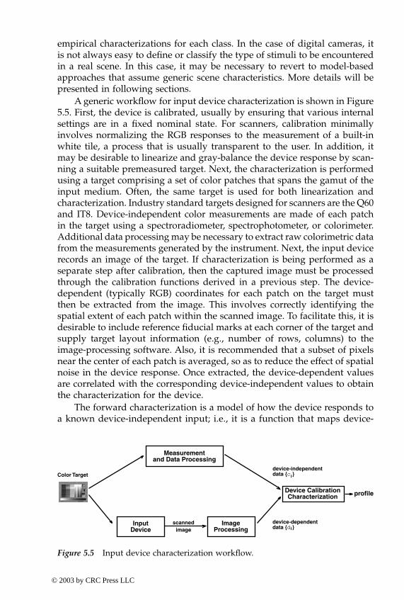
A generic workflow for input device characterization is shown in Figure5.5. First, the device is calibrated, usually by ensuring that various internalsettings are in a fixed nominal state. For scanners, calibration minimallyinvolves normalizing the RGB responses to the measurement of a built-inwhite tile, a process that is usually transparent to the user. In addition, itmay be desirable to linearize and gray-balance the device response by scan-ning a suitable premeasured target. Next, the characterization is performedusing a target comprising a set of color patches that spans the gamut of theinput medium. Often, the same target is used for both linearization andcharacterization. Industry standard targets designed for scanners are the Q60and IT8. Device-independent color measurements are made of each patchin the target using a spectroradiometer, spectrophotometer, or colorimeter.Additional data processing may be necessary to extract raw colorimetric datafrom the measurements generated by the instrument. Next, the input devicerecords an image of the target. If characterization is being performed as aseparate step after calibration, then the captured image must be processedthrough the calibration functions derived in a previous step. The device-dependent (typically RGB) coordinates for each patch on the target mustthen be extracted from the image. This involves correctly identifying thespatial extent of each patch within the scanned image. To facilitate this, it isdesirable to include reference fiducial marks at each corner of the target andsupply target layout information (e.g., number of rows, columns) to theimage-processing software. Also, it is recommended that a subset of pixelsnear the center of each patch is averaged, so as to reduce the effect of spatialnoise in the device response. Once extracted, the device-dependent valuesare correlated with the corresponding device-independent values to obtainthe characterization for the device.
The forward characterization is a model of how the device responds toa known device-independent input; i.e., it is a function that maps device-
Device CalibrationCharacterization
Color Target
InputDevice
scannedimage
ImageProcessing
device-independentdata {c }
device-dependentdata {d }
Measurementand Data Processing
i
i
profile
Figure 5.5 Input device characterization workflow.
-ColorBook Page 280 Wednesday, November 13, 2002 10:55 AM
© 2003 by CRC Press LLC
Chapter five: Device characterization 281
independent measurements to the resulting device signals. The inverse func-tion compensates for the device characteristics and maps device signals tocorresponding device-independent values. Model-based techniques esti-mate the forward function, which is then inverted using analytic or numer-ical approaches. Empirical techniques derive both the forward and inversefunctions.
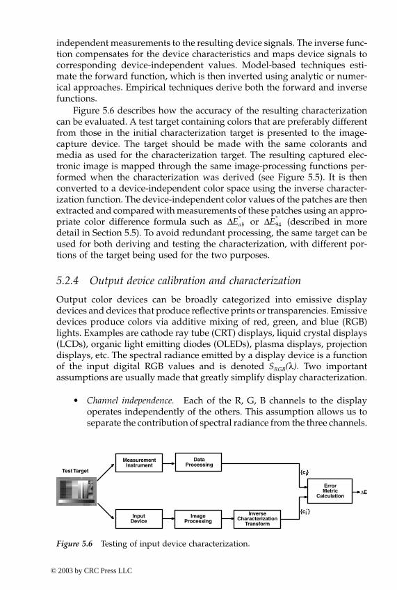
Figure 5.6 describes how the accuracy of the resulting characterizationcan be evaluated. A test target containing colors that are preferably differentfrom those in the initial characterization target is presented to the image-capture device. The target should be made with the same colorants andmedia as used for the characterization target. The resulting captured elec-tronic image is mapped through the same image-processing functions per-formed when the characterization was derived (see Figure 5.5). It is thenconverted to a device-independent color space using the inverse character-ization function. The device-independent color values of the patches are thenextracted and compared with measurements of these patches using an appro-priate color difference formula such as ∆ or ∆ (described in moredetail in Section 5.5). To avoid redundant processing, the same target can beused for both deriving and testing the characterization, with different por-tions of the target being used for the two purposes.
5.2.4 Output device calibration and characterization
Output color devices can be broadly categorized into emissive displaydevices and devices that produce reflective prints or transparencies. Emissivedevices produce colors via additive mixing of red, green, and blue (RGB)lights. Examples are cathode ray tube (CRT) displays, liquid crystal displays(LCDs), organic light emitting diodes (OLEDs), plasma displays, projectiondisplays, etc. The spectral radiance emitted by a display device is a functionof the input digital RGB values and is denoted SRGB(λ). Two importantassumptions are usually made that greatly simplify display characterization.
• Channel independence. Each of the R, G, B channels to the displayoperates independently of the others. This assumption allows us toseparate the contribution of spectral radiance from the three channels.
Test Target
MeasurementInstrument
InputDevice
ErrorMetric
Calculation∆E
{c }
{c }
i
i
DataProcessing
ImageProcessing
InverseCharacterization
Transform
Figure 5.6 Testing of input device characterization.
Eab* E94
*
-ColorBook Page 281 Wednesday, November 13, 2002 10:55 AM
© 2003 by CRC Press LLC
282 Digital Color Imaging Handbook
SRGB(λ) = SR(λ) + SG(λ) + SB(λ) (5.7)
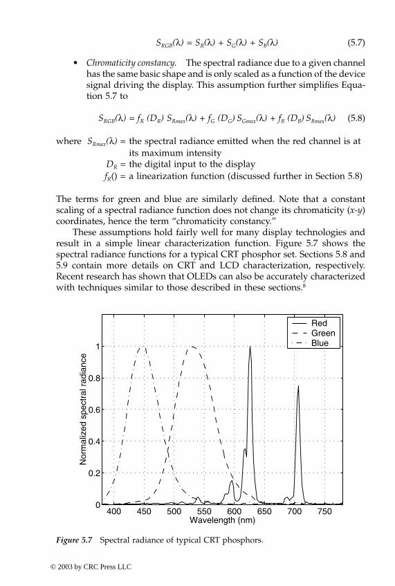
• Chromaticity constancy. The spectral radiance due to a given channelhas the same basic shape and is only scaled as a function of the devicesignal driving the display. This assumption further simplifies Equa-tion 5.7 to
SRGB(λ) = fR (DR) SRmax(λ) + fG (DG) SGmax(λ) + fB (DB) SBmax(λ) (5.8)
where SRmax(λ) = the spectral radiance emitted when the red channel is at its maximum intensity
DR = the digital input to the displayfR() = a linearization function (discussed further in Section 5.8)
The terms for green and blue are similarly defined. Note that a constantscaling of a spectral radiance function does not change its chromaticity (x-y)coordinates, hence the term “chromaticity constancy.”
These assumptions hold fairly well for many display technologies andresult in a simple linear characterization function. Figure 5.7 shows thespectral radiance functions for a typical CRT phosphor set. Sections 5.8 and5.9 contain more details on CRT and LCD characterization, respectively.Recent research has shown that OLEDs can also be accurately characterizedwith techniques similar to those described in these sections.8
400 450 500 550 600 650 700 7500
0.2
0.4
0.6
0.8
1
Wavelength (nm)
Nor
mal
ized
spe
ctra
l rad
ianc
e
RedGreenBlue
Figure 5.7 Spectral radiance of typical CRT phosphors.
-ColorBook Page 282 Wednesday, November 13, 2002 10:55 AM
© 2003 by CRC Press LLC
Chapter five: Device characterization 283
Printing devices produce color via subtractive color mixing in which abase medium for the colorants (usually paper or transparency) reflects ortransmits most of the light at all visible wavelengths, and different spectraldistributions are produced by combining cyan, magenta, and yellow (CMY)colorants to selectively remove energy from the red, green, and blue portionsof the electromagnetic spectrum of a light source. Often, a black colorant (K)is used both to increase the capability to produce dark colors and to reducethe use of expensive color inks. Photographic prints and transparencies andoffset, laser, and inkjet printing use subtractive color.
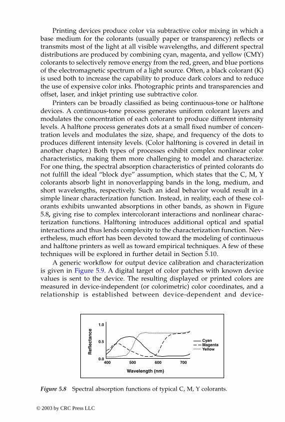
Printers can be broadly classified as being continuous-tone or halftonedevices. A continuous-tone process generates uniform colorant layers andmodulates the concentration of each colorant to produce different intensitylevels. A halftone process generates dots at a small fixed number of concen-tration levels and modulates the size, shape, and frequency of the dots toproduces different intensity levels. (Color halftoning is covered in detail inanother chapter.) Both types of processes exhibit complex nonlinear colorcharacteristics, making them more challenging to model and characterize.For one thing, the spectral absorption characteristics of printed colorants donot fulfill the ideal “block dye” assumption, which states that the C, M, Ycolorants absorb light in nonoverlapping bands in the long, medium, andshort wavelengths, respectively. Such an ideal behavior would result in asimple linear characterization function. Instead, in reality, each of these col-orants exhibits unwanted absorptions in other bands, as shown in Figure5.8, giving rise to complex intercolorant interactions and nonlinear charac-terization functions. Halftoning introduces additional optical and spatialinteractions and thus lends complexity to the characterization function. Nev-ertheless, much effort has been devoted toward the modeling of continuousand halftone printers as well as toward empirical techniques. A few of thesetechniques will be explored in further detail in Section 5.10.
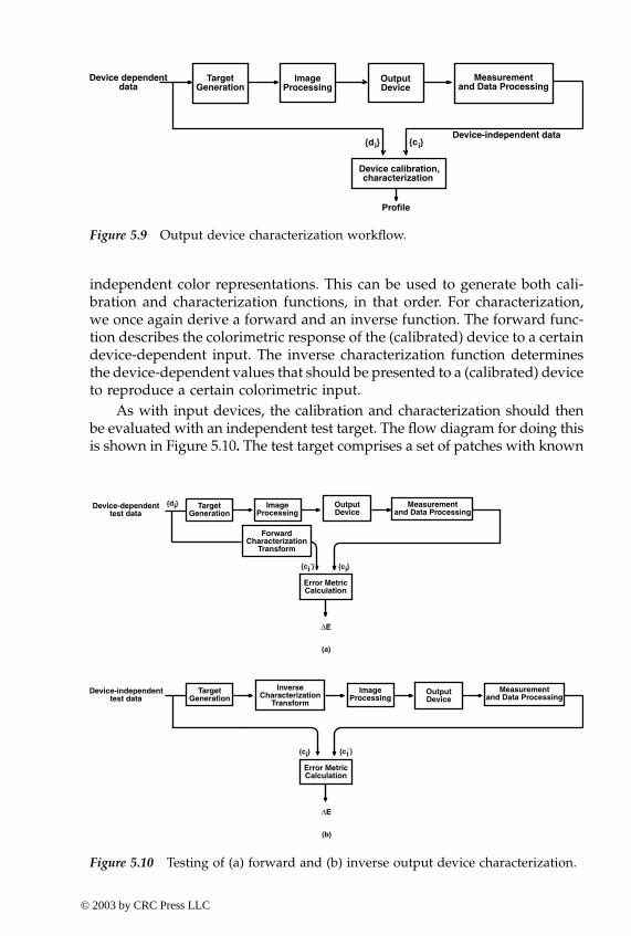
A generic workflow for output device calibration and characterizationis given in Figure 5.9. A digital target of color patches with known devicevalues is sent to the device. The resulting displayed or printed colors aremeasured in device-independent (or colorimetric) color coordinates, and arelationship is established between device-dependent and device-
400 500 600 7000.0
0.5
1.0
Wavelength (nm)
Ref
lect
ance
CyanMagentaYellow
Figure 5.8 Spectral absorption functions of typical C, M, Y colorants.
-ColorBook Page 283 Wednesday, November 13, 2002 10:55 AM
© 2003 by CRC Press LLC
284 Digital Color Imaging Handbook
independent color representations. This can be used to generate both cali-bration and characterization functions, in that order. For characterization,we once again derive a forward and an inverse function. The forward func-tion describes the colorimetric response of the (calibrated) device to a certaindevice-dependent input. The inverse characterization function determinesthe device-dependent values that should be presented to a (calibrated) deviceto reproduce a certain colorimetric input.
As with input devices, the calibration and characterization should thenbe evaluated with an independent test target. The flow diagram for doing thisis shown in Figure 5.10. The test target comprises a set of patches with known
Device-independent data
Device dependentdata
TargetGeneration
OutputDevice
Measurementand Data Processing
ImageProcessing
Device calibration,characterization
{d }i {c }i
Profile
Figure 5.9 Output device characterization workflow.
Device-dependenttest data
TargetGeneration
ImageProcessing
OutputDevice
ForwardCharacterization
Transform
Error MetricCalculation
∆E
(a)
{d }
{c }{c }
Device-independenttest data
TargetGeneration
Error MetricCalculation
∆E
(b)
{c }
InverseCharacterization
Transform
{c }
i
i i
i i
Measurementand Data Processing
ImageProcessing
OutputDevice
Measurementand Data Processing
Figure 5.10 Testing of (a) forward and (b) inverse output device characterization.
-ColorBook Page 284 Wednesday, November 13, 2002 10:55 AM
© 2003 by CRC Press LLC
Chapter five: Device characterization 285
device-independent coordinates. If calibration is being tested, this target isprocessed through the calibration functions and rendered to the device. Ifcharacterization is being evaluated, the target is processed through both thecharacterization and calibration function and rendered to the device. Theresulting output is measured in device-independent coordinates and com-pared with the original target values. Once again, the comparison is to becarried out with an appropriate color difference formula such as ∆ or ∆ .
An important component of the color characteristics of an output deviceis its color gamut, namely the volume of colors in three-dimensional colori-metric space that is physically achievable by the device. Of particular impor-tance is the gamut surface, as this is used in gamut mapping algorithms.This information can easily be derived from the characterization process.Details of gamut surface calculation are provided in the chapter on gamutmapping.
5.3 Characterization targets and measurement techniques The generation and measurement of color targets is an important componentof device characterization. Hence, a separate section is devoted to this topic.
5.3.1 Color target design
The design of a color target involves several factors. First is the set of colo-rants and underlying medium of the target. In the case of input devices, thecharacterization target is created offline (i.e., it is not part of the character-ization process) with colorants and media that are representative of whatthe device is likely to capture. For example, for scanner characterization,photographic and offset lithographic processes are commonly used to createtargets on reflective or transmissive media. In the case of output devices,target generation is part of the characterization process and should be carriedout using the same colorants and media that will be used for final colorrendition.
The second factor is the choice of color patches. Typically, the patchesare chosen to span the desired range of the colors to be captured (in thecase of input devices) or rendered (in the case of output devices). Often,critical memory colors are included, such as flesh tones and neutrals. Theoptimal choice of patches is logically a function of the particular algorithmor model that will be used to generate the calibration or characterizationfunction. Nevertheless, a few targets have been adopted as industry stan-dards, and they accommodate a variety of characterization techniques. Forinput device characterization, these include the CGATS/ANSI IT8.7/1 andIT8.7/2 targets for transmission and reflection media respectively(http://webstore.ansi.org/ansidocstore); the Kodak photographic Q60 tar-get, which is based on the IT8 standards and is made with Ektachrome dyeson Ektacolor paper (www.kodak.com); the GretagMacbeth ColorCheckerchart (www.munsell.com); and ColorChecker DC version for digital cam-
Eab* E94
*
-ColorBook Page 285 Wednesday, November 13, 2002 10:55 AM
© 2003 by CRC Press LLC
286 Digital Color Imaging Handbook
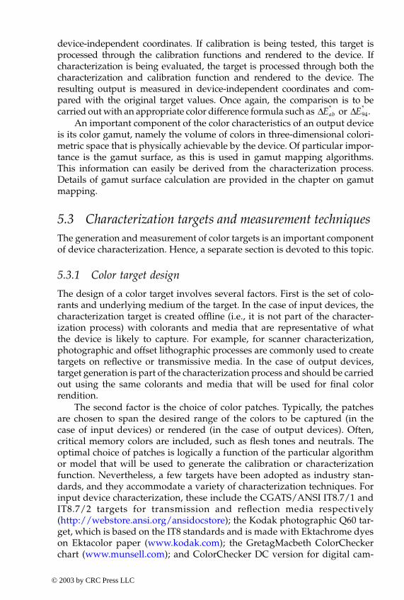
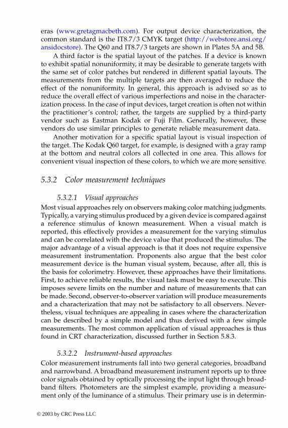
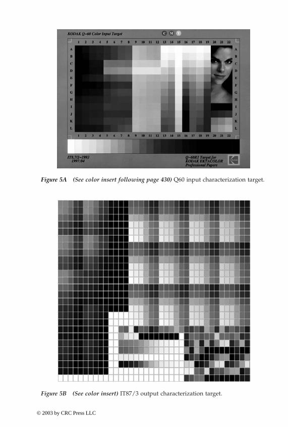
eras (www.gretagmacbeth.com). For output device characterization, thecommon standard is the IT8.7/3 CMYK target (http://webstore.ansi.org/ansidocstore). The Q60 and IT8.7/3 targets are shown in Plates 5A and 5B.
A third factor is the spatial layout of the patches. If a device is knownto exhibit spatial nonuniformity, it may be desirable to generate targets withthe same set of color patches but rendered in different spatial layouts. Themeasurements from the multiple targets are then averaged to reduce theeffect of the nonuniformity. In general, this approach is advised so as toreduce the overall effect of various imperfections and noise in the character-ization process. In the case of input devices, target creation is often not withinthe practitioner’s control; rather, the targets are supplied by a third-partyvendor such as Eastman Kodak or Fuji Film. Generally, however, thesevendors do use similar principles to generate reliable measurement data.
Another motivation for a specific spatial layout is visual inspection ofthe target. The Kodak Q60 target, for example, is designed with a gray rampat the bottom and neutral colors all collected in one area. This allows forconvenient visual inspection of these colors, to which we are more sensitive.
5.3.2 Color measurement techniques
5.3.2.1 Visual approachesMost visual approaches rely on observers making color matching judgments.Typically, a varying stimulus produced by a given device is compared againsta reference stimulus of known measurement. When a visual match isreported, this effectively provides a measurement for the varying stimulusand can be correlated with the device value that produced the stimulus. Themajor advantage of a visual approach is that it does not require expensivemeasurement instrumentation. Proponents also argue that the best colormeasurement device is the human visual system, because, after all, this isthe basis for colorimetry. However, these approaches have their limitations.First, to achieve reliable results, the visual task must be easy to execute. Thisimposes severe limits on the number and nature of measurements that canbe made. Second, observer-to-observer variation will produce measurementsand a characterization that may not be satisfactory to all observers. Never-theless, visual techniques are appealing in cases where the characterizationcan be described by a simple model and thus derived with a few simplemeasurements. The most common application of visual approaches is thusfound in CRT characterization, discussed further in Section 5.8.3.
5.3.2.2 Instrument-based approachesColor measurement instruments fall into two general categories, broadbandand narrowband. A broadband measurement instrument reports up to threecolor signals obtained by optically processing the input light through broad-band filters. Photometers are the simplest example, providing a measure-ment only of the luminance of a stimulus. Their primary use is in determin-
-ColorBook Page 286 Wednesday, November 13, 2002 10:55 AM
© 2003 by CRC Press LLC
Chapter five: Device characterization 287
Figure 5A (See color insert following page 430) Q60 input characterization target.
Figure 5B (See color insert) IT87/3 output characterization target.
05 Page 287 Tuesday, November 19, 2002 2:14 PM
© 2003 by CRC Press LLC
288 Digital Color Imaging Handbook
ing the nonlinear calibration function of displays (discussed in Section 5.8).Densitometers are an example of broadband instruments that measure opti-cal density of light filtered through red, green, and blue filters. Colorimetersare another example of broadband instruments that directly report tristim-ulus (XYZ) values and their derivatives such as CIELAB. In the narrowbandcategory fall instruments that report spectral data of dimensionality signif-icantly larger than three. Spectrophotometers and spectroradiometers areexamples of narrowband instruments. These instruments typically recordspectral reflectance and radiance, respectively, within the visible spectrumin increments ranging from 1 to 10 nm, resulting in 30 to 300 channels. Theyalso have the ability to internally calculate and report tristimulus coordinatesfrom the narrowband spectral data. Spectroradiometers can measure bothemissive and reflective stimuli, while spectrophotometers can measure onlyreflective stimuli.
The main advantages of broadband instruments such as densitometersand colorimeters are that they are inexpensive and can read out data at veryhigh rates. However, the resulting measurement is only an approximationof the true tristimulus signal, and the quality of this approximation varieswidely, depending on the nature of the stimulus being measured. Accuratecolorimetric measurement of arbitrary stimuli under arbitrary illuminationand viewing conditions requires spectral measurements afforded by themore expensive narrowband instruments. Traditionally, the printing indus-try has satisfactorily relied on densitometers to make color measurementsof prints made by offset ink. However, given the larger variety of colorants,printing technologies, and viewing conditions likely to be encountered intoday’s digital color imaging business, the use of spectral measurementinstruments is strongly recommended for device characterization. Fortu-nately, the steadily declining cost of spectral instrumentation makes this arealistic prospect.
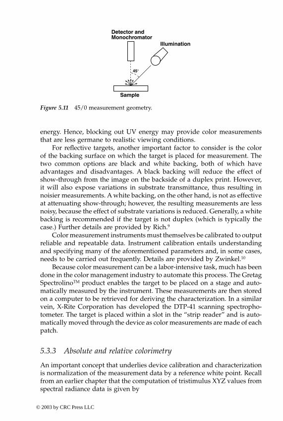
Instruments measuring reflective or transmissive samples possess aninternal light source that illuminates the sample. Common choices forsources are tungsten-halogen bulbs as well as xenon and pulsed-xenonsources. An important consideration in reflective color measurement is theoptical geometry used to illuminate the sample and capture the reflectedlight. A common choice is the 45/0 geometry, shown in Figure 5.11. (Thetwo numbers are the angles with respect to the surface normal of the incidentillumination and detector respectively.) This geometry is intended to mini-mize the effect of specular reflection and is also fairly representative of theconditions under which reflection prints are viewed. Another considerationis the measurement aperture, typically set between 3 and 5 mm. Anotherfeature, usually offered at extra cost with the spectrophotometer, is a filterthat blocks out ultraviolet (UV) light emanated by the internal source. Thefilter serves to reduce the amount of fluorescence in the prints that is causedby the UV light. Before using such a filter, however, it must be rememberedthat common viewing environments are illuminated by light sources (e.g.,sunlight, fluorescent lamps) that also exhibit a significant amount of UV
-ColorBook Page 288 Wednesday, November 13, 2002 10:55 AM
© 2003 by CRC Press LLC
Chapter five: Device characterization 289
energy. Hence, blocking out UV energy may provide color measurementsthat are less germane to realistic viewing conditions.
For reflective targets, another important factor to consider is the colorof the backing surface on which the target is placed for measurement. Thetwo common options are black and white backing, both of which haveadvantages and disadvantages. A black backing will reduce the effect ofshow-through from the image on the backside of a duplex print. However,it will also expose variations in substrate transmittance, thus resulting innoisier measurements. A white backing, on the other hand, is not as effectiveat attenuating show-through; however, the resulting measurements are lessnoisy, because the effect of substrate variations is reduced. Generally, a whitebacking is recommended if the target is not duplex (which is typically thecase.) Further details are provided by Rich.9
Color measurement instruments must themselves be calibrated to outputreliable and repeatable data. Instrument calibration entails understandingand specifying many of the aforementioned parameters and, in some cases,needs to be carried out frequently. Details are provided by Zwinkel.10
Because color measurement can be a labor-intensive task, much has beendone in the color management industry to automate this process. The GretagSpectrolinoTM product enables the target to be placed on a stage and auto-matically measured by the instrument. These measurements are then storedon a computer to be retrieved for deriving the characterization. In a similarvein, X-Rite Corporation has developed the DTP-41 scanning spectropho-tometer. The target is placed within a slot in the “strip reader” and is auto-matically moved through the device as color measurements are made of eachpatch.
5.3.3 Absolute and relative colorimetry
An important concept that underlies device calibration and characterizationis normalization of the measurement data by a reference white point. Recallfrom an earlier chapter that the computation of tristimulus XYZ values fromspectral radiance data is given by
Sample
Illumination
Detector andMonochromator
45°
Figure 5.11 45/0 measurement geometry.
-ColorBook Page 289 Wednesday, November 13, 2002 10:55 AM
© 2003 by CRC Press LLC
290 Digital Color Imaging Handbook
(5.9)
where = color matching functionsV = set of visible wavelengthsK = a normalization constant
In absolute colorimetry, K is a constant, expressed in terms of the maximumefficacy of radiant power, equal to 683 lumens/W. In relative colorimetry, Kis chosen such that Y = 100 for a chosen reference white point.
(5.10)
where Sw(λ) = the spectral radiance of the reference white stimulus.For reflective stimuli, radiance Sw(λ) is a product of incident illumination
I(λ) and spectral reflectance Rw(λ) of a white sample. The latter is usuallychosen to be a perfect diffuse reflector (i.e., Rw(λ) = 1) so that Sw(λ) = I(λ) inEquation 5.10.
There is an additional white-point normalization to be considered. Theconversion from tristimulus values to appearance coordinates such asCIELAB or CIELUV requires the measurement of a reference white stimulusand an appropriate scaling of all tristimulus values by this white point. Inthe case of emissive display devices, the white point is the measurement ofthe light emanated by the display device when the driving RGB signals areat their maximal values (e.g., DR = DG = DB = 255 for 8-bit input). In the caseof reflective samples, the white point is obtained by measuring the lightemanating from a reference white sample illuminated by a specified lightsource. If an ideal diffuse reflector is used as the white sample, we refer tothe measurements as being in media absolute colorimetric coordinates. If a par-ticular medium (e.g., paper) is used as the stimulus, we refer to the mea-surements as being in media relative colorimetric coordinates. Conversionsbetween media absolute and relative colorimetry are achieved with a white-point normalization model such as the von Kries formula.
To get an intuitive understanding of the effect of media absolute vs.relative colorimetry, consider an example of scan-to-print reproduction of acolor image. Suppose the image being scanned is a photograph whosemedium typically exhibits a yellowish cast. This image is to be printed ona xerographic printer, which typically uses a paper with fluorescent whit-eners and is thus lighter and bluer than the photographic medium. Theimage is scanned, processed through both scanner and printer characteriza-tion functions, and printed. If the characterizations are built using mediaabsolute colorimetry, the yellowish cast of the photographic medium is
X K S λ( )x λ( )∂λ, YλεV∫ K S λ( )y∂λ, Z
λεV∫ K S λ( )z λ( )∂λ
λεV∫= = =
x λ( ), y λ( ), z λ( )
K 100
Sw λ( )λεV∫ y λ( )∂λ
-----------------------------------------=
-ColorBook Page 290 Wednesday, November 13, 2002 10:55 AM
© 2003 by CRC Press LLC
Chapter five: Device characterization 291
preserved in the xerographic reproduction. On the other hand, with mediarelative colorimetry, the “yellowish white” of the photographic mediummaps directly to the “bluish white” of the xerographic medium under thepremise that the human visual system adapts and perceives each mediumas “white” when viewed in isolation. Arguments can be made for bothmodes, depending on the application. Side-by-side comparisons of originaland reproduction may call for media absolute characterization. If the repro-duction is to be viewed in isolation, it is probably preferable to exploit visualwhite-point adaptation and employ relative colorimetry. To this end, theICC specification supports both media absolute and media relative modesin its characterization tables.
Finally, we remark that, while a wide variety of standard illuminantscan be selected for deriving the device characterization function, the mostcommon choices are CIE daylight illuminants D5000 (typically used forreflection prints) and D6500 (typically used for the white point of displays).
5.4 Multidimensional data fitting and interpolationAnother critical component underlying device characterization is multidi-mensional data fitting and interpolation. This topic is treated in generalmathematical terms in this section. Application to specific devices will bediscussed in ensuing sections.
Generally, the data samples generated by the characterization process inboth device-dependent and device-independent spaces will constitute onlya small subset of all possible digital values that could be encountered ineither space. One reason for this is that the total number of possible samplesin a color space is usually prohibitively large for direct measurement of thecharacterization function. As an example, for R, G, B signals representedwith 8-bit precision, the total number of possible colors is 224 = 16,777,216;clearly an unreasonable amount of data to be acquired manually. However,because the final characterization function will be used for transformingarbitrary image data, it needs to be defined for all possible inputs withinsome expected domain. To accomplish this, some form of data fitting orinterpolation must be performed on the characterization samples. In model-based characterization, the underlying physical model serves to perform thefitting or interpolation for the forward characterization function. With empir-ical approaches, mathematical techniques may be used to perform datafitting or interpolation. Some of the common mathematical approaches arediscussed in this section.
The fitting or interpolation concept can be formalized as follows. Definea set of T m-dimensional device-dependent color samples {di} ∈ Rm, i = 1,. . . , T generated by the characterization process. Define the correspondingset of n-dimensional device-independent samples {ci} ∈ Rn, i = 1, . . . , T. Forthe majority of characterization functions, n = 3, and m = 3 or 4. We willoften refer to the pair ({di}, {ci}) as the set of training samples. From this set,we wish to evaluate one or both of the following functions:
-ColorBook Page 291 Wednesday, November 13, 2002 10:55 AM
© 2003 by CRC Press LLC
292 Digital Color Imaging Handbook
• f: F ∈ Rm → Rn, mapping device-dependent data within a domain Fto device-independent color space
• g: G ∈ Rn → Rm, mapping device-independent data within a domainG to device-dependent color space
In interpolation schemes, the error of the functional approximation isidentically zero at all the training samples, i.e., f(di) = ci, and g(ci) = di, i =1, . . . , T.
In fitting schemes, this condition need not hold. Rather, the fitting func-tion is designed to minimize an error criterion between the training samplesand the functional approximations at these samples. Formally,
(5.11)
where E1 and E2 are suitably chosen error criteria.A common approach is to pick a parametric form for f (or g) and mini-
mize the mean squared error metric, given by
(5.12)
An analogous expression holds for E2. The minimization is performed withrespect to the parameters of the function f or g.
Unfortunately, most of the data fitting and interpolation approaches tobe discussed shortly are too computationally expensive for the processing oflarge amounts of image pixel data in real time. The most common way toaddress this problem is to first evaluate the complex fitting or interpolationfunctions at a regular lattice of points in the input space and build a multi-dimensional lookup table (LUT). A fast interpolation technique such as tri-linear or tetrahedral interpolation is then used to transform image data usingthis LUT. The subject of fast LUT interpolation on regular lattices is treatedin a later chapter. Here, we will focus on the fitting and interpolation methodsused to initially approximate the characterization function and build the LUT.
Often, it is necessary to evaluate the functions f and g within domains Fand G that are outside of the volumes spanned by the training data {di} and{ci}. An example is shown in Figure 5.12 for printer characterization mappingCIELAB to CMY. A two-dimensional projection of CIELAB space is shown,with a set of training samples {ci} indicated by “x.” Device-dependent CMYvalues {di} are known at each of these points. The shaded area enclosed bythese samples is the range of colors achievable by the printer, namely its colorgamut. From these data, the inverse printer characterization function fromCIELAB to CMY is to be evaluated at each of the lattice points lying on thethree-dimensional lookup table grid (projected as a two-dimensional grid in
ff opt minE1arg ci, f di( )(= i 1,… ,T= ); gopt minE2arg di,g ci( )(= i 1,… ,T= )
g
E11T---
i 1=
T
∑ ci f di( )– || ||2
=
-ColorBook Page 292 Wednesday, November 13, 2002 10:55 AM
© 2003 by CRC Press LLC
Chapter five: Device characterization 293
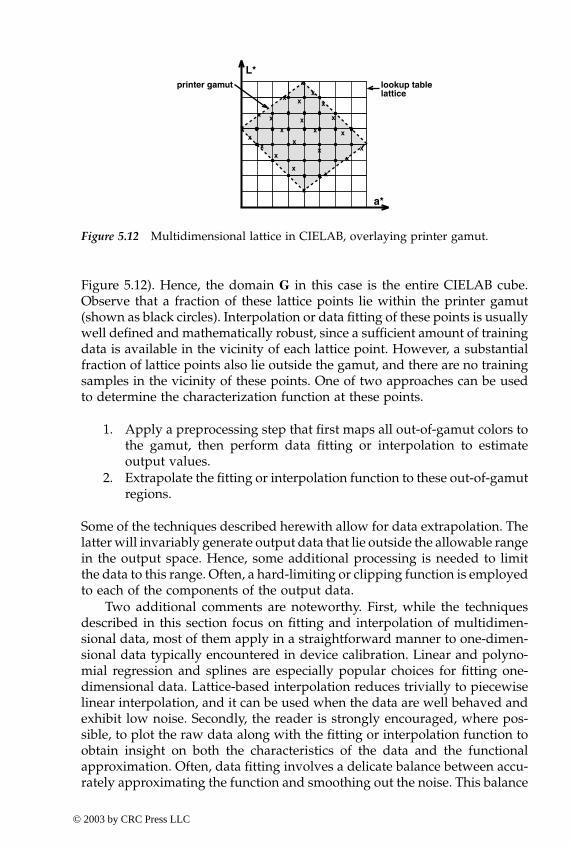
Figure 5.12). Hence, the domain G in this case is the entire CIELAB cube.Observe that a fraction of these lattice points lie within the printer gamut(shown as black circles). Interpolation or data fitting of these points is usuallywell defined and mathematically robust, since a sufficient amount of trainingdata is available in the vicinity of each lattice point. However, a substantialfraction of lattice points also lie outside the gamut, and there are no trainingsamples in the vicinity of these points. One of two approaches can be usedto determine the characterization function at these points.
1. Apply a preprocessing step that first maps all out-of-gamut colors tothe gamut, then perform data fitting or interpolation to estimateoutput values.
2. Extrapolate the fitting or interpolation function to these out-of-gamutregions.
Some of the techniques described herewith allow for data extrapolation. Thelatter will invariably generate output data that lie outside the allowable rangein the output space. Hence, some additional processing is needed to limitthe data to this range. Often, a hard-limiting or clipping function is employedto each of the components of the output data.
Two additional comments are noteworthy. First, while the techniquesdescribed in this section focus on fitting and interpolation of multidimen-sional data, most of them apply in a straightforward manner to one-dimen-sional data typically encountered in device calibration. Linear and polyno-mial regression and splines are especially popular choices for fitting one-dimensional data. Lattice-based interpolation reduces trivially to piecewiselinear interpolation, and it can be used when the data are well behaved andexhibit low noise. Secondly, the reader is strongly encouraged, where pos-sible, to plot the raw data along with the fitting or interpolation function toobtain insight on both the characteristics of the data and the functionalapproximation. Often, data fitting involves a delicate balance between accu-rately approximating the function and smoothing out the noise. This balance
a*
L*lookup tablelattice
xx
x
x
x
x
x
x
x
x
x
x
xx
x
xx
x
x
x
x
x
printer gamut
x
Figure 5.12 Multidimensional lattice in CIELAB, overlaying printer gamut.
-ColorBook Page 293 Wednesday, November 13, 2002 10:55 AM
© 2003 by CRC Press LLC
294 Digital Color Imaging Handbook
is difficult to achieve by examining only a single numerical error metric andis significantly aided by visualizing the entire dataset in combination withthe fitting functions.
5.4.1 Linear least-squares regression
This very common data fitting approach is used widely in color imaging,particularly in device characterization and modeling. The problem is formu-lated as follows. Denote
d
and
c
to be the input and output color vectors,respectively, for a characterization function. Specifically,
d
is a 1
¥
m
vector,and
c
is a 1
¥
n
vector. We wish to approximate the characterization functionby the linear relationship
c
=
d
·
A
.The matrix
A
is of dimension
m
¥
n
and is derived by minimizing themean squared error of the linear fit to a set of training samples, {
d
i
,
c
i
},
i
=1, . . . ,
T
. Mathematically, the optimal
A
is given by
(5.13)
To continue the formulation, it is convenient to collect the samples {
c
i
} intoa
T
¥
n
matrix
C =
[
c
1
, . . . ,
c
T
], and {
d
i
} into a
T
¥
m
matrix
D
= [
d
1
,
. . .
,
d
T
].The linear relationship is given by
C
=
D
·
A
. The optimal
A
is given by
A
=
D
†
C
, where
D
† is the generalized inverse (sometimes known as theMoore–Penrose pseudo-inverse) of
D
. In the case where
D
t
D
is invertible,the optimum
A
is given by
A
= (
D
t
D
)
–
1
D
t
C
(5.14)
See Appendix 5.A for the derivation and numerical computation of thisleast-squares solution. It is important to understand the conditions for whichthe solution to Equation 5.14 exists. If
T
<
m,
we have an underdeterminedsystem of equations with no unique solution. The mathematical consequenceof this is that the matrix
D
t
D
is of insufficient rank and is thus not invertible.Thus, we need at least as many samples as the dimensionality of the inputdata. If
T
=
m,
we have an exact solution for
A
that results in the squarederror metric being identically zero. If
T
>
m
(the preferred case), Equation5.14 provides a least-squares solution to an overdetermined system of equa-tions. Note that linear regression affords a natural means of extrapolationfor input data
d
lying outside the domain of the training samples. As men-tioned earlier, some form of clipping will be needed to limit such extrapo-lated outputs to their allowable range.
5.4.2 Weighted least-squares regression
The standard least-squares regression can be extended to minimize aweighted error criterion,
AAopt minarg 1
T---
i 1=
T
 ci di� A || ||2
Ó þÌ ýÏ ¸
=
05 Page 294 Monday, November 18, 2002 8:22 AM
© 2003 by CRC Press LLC
Chapter five: Device characterization 295
(5.15)
where wi = positive-valued weights that indicate the relative importance of the ith data point, {di, ci}.
Adopting the notation in Section 5.4.1, a straightforward extension of Appen-dix 5.A results in the following optimum solution:
A = (DtWD)–1 Dt WC (5.16)
where W is a T × T diagonal matrix with diagonal entries wi.The resulting fit will be biased toward achieving greater accuracy at the
more heavily weighted samples. This can be a useful feature in device char-acterization when, for example, we wish to assign greater importance tocolors in certain regions of color space (e.g., neutrals, fleshtones, etc.). Asanother example, in spectral regression, it may be desirable to assign greaterimportance to certain wavelengths than others.
5.4.3 Polynomial regression
This is a special form of least-squares fitting wherein the characterizationfunction is approximated by a polynomial. We will describe the formulationusing, as an example, a scanner characterization mapping device RGB spaceto XYZ tristimulus space. The formulation is conceptually identical for inputand output devices and for the forward and inverse functions.
The third-order polynomial approximation for a transformation fromRGB to XYZ space is given by
(5.17)
where wX,l, etc. = polynomial weightsl = a unique index for each combination of i, j, k
In practice, several of the terms in Equation 5.17 are eliminated (i.e., the weightsw are set to zero) so as to control the number of degrees of freedom in thepolynomial. Two common examples, a linear and third-order approximation,
Aopt minarg 1T--- wi ci diA– 2
i 1=
T
∑
=
X wX ,lRiGjBk;
k 0=
3
∑j 0=
3
∑i 0=
3
∑ Y wY l,k 0=
3
∑j 0=
3
∑i 0=
3
∑ RiGjBk;= =
Z wZ l, k 0=
3
∑ RiGjBk
j 0=
3
∑i 0=
3
∑=
-ColorBook Page 295 Wednesday, November 13, 2002 10:55 AM
© 2003 by CRC Press LLC
296 Digital Color Imaging Handbook
are given below. For brevity, only the X term is defined; analogous definitionshold for Y and Z.
X = wX,0R + wX,1G + wX,2B (5.18a)
X = wX,0 + wX,1R + wX,2G + wX,3B + wX,4RG + wX,5GB + wX,6RB + wX,7R2 + wX,8G2 + wX,9B2 + wX,10RGB (5.18b)
In matrix-vector notation, Equation 5.17 can be written as
(5.19)
or more compactly,
c = p · A (5.20)
where c = output XYZ vector p = 1 × Q vector of Q polynomial terms derived from the input RGB
vector dA = Q × 3 matrix of polynomial weights to be optimized
In the complete form, Q = 64. However, with the more common simplifiedapproximations in Equation 5.18, this number is significantly smaller; i.e., Q= 3 and Q = 11, respectively.
Note from Equation 5.20 that the polynomial regression problem hasbeen cast into a linear least-squares problem with suitable preprocessing ofthe input data d into the polynomial vector p. The optimal A is now given by
(5.21)
Collecting the samples {ci} into a T × 3 matrix C = [c1, . . . , cT], and {pi} intoa T × Q matrix P = [p1, . . . , pT], we have the relationship C = P · A. Followingthe formulation in Section 5.4.1, the optimal solution for A is given by
A = (PtP)–1 PtC (5.22)
For the Q × Q matrix (PtP) to be invertible, we now require that T ≥ Q.
X Y Z 1 R G … R3 G3 B3
wX ,0 wY ,0 wZ ,0
wX ,1 wY ,1 wz ,3
…wX ,63 wY ,63 wZ ,63
=
Aopt minarg 1T--- ci piA– 2
i 1=
T
∑
=A
-ColorBook Page 296 Wednesday, November 13, 2002 10:55 AM
© 2003 by CRC Press LLC
Chapter five: Device characterization 297
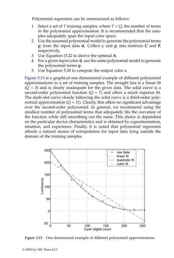
Polynomial regression can be summarized as follows:
1. Select a set of T training samples, where T > Q, the number of termsin the polynomial approximation. It is recommended that the sam-ples adequately span the input color space.
2. Use the assumed polynomial model to generate the polynomial termspi from the input data di. Collect ci and pi into matrices C and P,respectively.
3. Use Equation (5.22 to derive the optimal A.4. For a given input color d, use the same polynomial model to generate
the polynomial terms p.5. Use Equation 5.20 to compute the output color c.
Figure 5.13 is a graphical one-dimensional example of different polynomialapproximations to a set of training samples. The straight line is a linear fit(Q = 3) and is clearly inadequate for the given data. The solid curve is asecond-order polynomial function (Q = 7) and offers a much superior fit.The dash–dot curve closely following the solid curve is a third-order poly-nomial approximation (Q = 11). Clearly, this offers no significant advantageover the second-order polynomial. In general, we recommend using thesmallest number of polynomial terms that adequately fits the curvature ofthe function while still smoothing out the noise. This choice is dependenton the particular device characteristics and is obtained by experimentation,intuition, and experience. Finally, it is noted that polynomial regressionaffords a natural means of extrapolation for input data lying outside thedomain of the training samples.
0 50 100 150 200 25050
0
50
100
150
200
250
Cyan digital count
Lum
inan
ce
raw datalinear fitquadratic fitcubic fit
Figure 5.13 One-dimensional example of different polynomial approximations.
-ColorBook Page 297 Wednesday, November 13, 2002 10:55 AM
© 2003 by CRC Press LLC
298 Digital Color Imaging Handbook
5.4.4 Distance-weighted techniques
The previous section described the use of a global polynomial function thatresults in the best overall fit to the training samples. In this section, wedescribe a class of techniques that also employ simple parametric functions;however, the parameters vary across color space to best fit the local charac-teristics of the training samples.
5.4.4.1 Shepard’s interpolationThis is a technique that can be applied to cases in which the input and outputspaces of the characterization function are of the same dimensionality. First,a crude approximation of the characterization function is defined: =fapprox(d). The main purpose of fapprox() is to bring the input data into theorientation of the output color space. (By “orientation,” it is meant that allRGB spaces are of the same orientation, as are all luminance–chrominancespaces, etc.) If both color spaces are already of the same orientation, e.g.,printer RGB and sRGB, we can simply let fapprox() be an identity function sothat = d. If, for example, the input and output spaces are scanner RGBand CIELAB, an analytic transformation from any colorimetric RGB (e.g.,sRGB) to CIELAB could serve as the crude approximation.
Next, given the training samples {di} and {ci} in the input and outputspace, respectively, we define error vectors between the crude approximationand true output values of these samples: . Shepard’sinterpolation for an arbitrary input color vector d is then given by11
(5.23)
where w() = weightsKw = a normalizing factor that ensures that these weights sum to
unity as follows:
(5.24)
The second term in Equation 5.23 is a correction for the residual errorbetween c and , and it is given by a weighted average of the error vectorsei at the training samples. The weighting function w() is chosen to beinversely proportional to the Euclidean distance between d and di so thattraining samples that are nearer the input point exhibit a stronger influencethan those that are further away. There are numerous candidates for w().One form that has been successfully used for printer and scanner character-ization is given by12
c
c
ei ci ci ,– 1, …,T= =
c c= Kw w d di–( )i 1=
T
∑ ei+
Kw1
w d di–( )i 1=
T
∑--------------------------------=
c
-ColorBook Page 298 Wednesday, November 13, 2002 10:55 AM
© 2003 by CRC Press LLC
Chapter five: Device characterization 299
(5.25)
where denotes Euclidean distance between vectors d and di, and ρand ε are parameters that dictate the relative influence of the training samplesas a function of their distance from the input point. As ρ increases, theinfluence of a training sample decays more rapidly as a function of itsdistance from the input point. As ε increases, the weights become less sen-sitive to distance, and the approach migrates from a local to a global approx-imation.
Note that, in the special case where ε = 0, the function in Equation 5.25has a singularity at d = di. This can be accommodated by adding a specialcondition to Equation 5.23.
(5.26)
where w() = given by Equation 5.25 with ε = 0t = a suitably chosen distance threshold that avoids the singularity
at d = di
Other choices of w() include the Gaussian and exponential functions.11 Notethat, depending on how the weights are chosen, Shepard’s algorithm can beused for both data fitting (i.e., Equation 5.23 and Equation 5.25 with ε > 0),and data interpolation, wherein the characterization function coincidesexactly at the training samples (i.e., Equation 5.26). Note also that this tech-nique allows for data extrapolation. As one moves farther away from thevolume spanned by the training samples, the distances and hencethe weights w() approach a constant. In the limit, the overall error correctionin Equation 5.23 is an unweighted average of the error vectors ei.
5.4.4.2 Local linear regressionIn this approach, the form of the characterization function that maps inputcolors d to output colors c is given by
c = d · Ad (5.27)
This looks very similar to the standard linear transformation, the importantdifference being that the matrix Ad now varies as a function of the inputcolor d (hence the term local linear regression). The optimal Ad is obtained bya distance-weighted least-squares regression,
w d di–( ) 1d di– p ε+
------------------------------=
d di–
c c Kw w d di–( )ei
i 1=
T
∑+ if d di– t≥( )
ci if d di– t<
=
d di–
-ColorBook Page 299 Wednesday, November 13, 2002 10:55 AM
© 2003 by CRC Press LLC
300 Digital Color Imaging Handbook
(5.28)
As with Shepard’s interpolation, the weighting function w() is inverselyproportional to the Euclidean distance , so training samples di thatare farther away from the input point d are assigned a smaller weight thannearby points. A form such as Equation 5.25 may be used.12 The solution isgiven by Equation 5.16 in Section 4.2, where the weights w(d – di) constitutethe diagonal terms of W. Note that because w() is a function of the inputvector d, Equation 5.16 must be recalculated for every input vector d. Hence,this is a computationally intensive algorithm. Fortunately, as noted earlier,this type of data fitting is not applied to image pixels in real time. Instead,it is used offline to create a multidimensional lookup table.
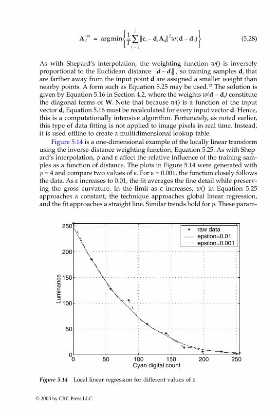
Figure 5.14 is a one-dimensional example of the locally linear transformusing the inverse-distance weighting function, Equation 5.25. As with Shep-ard’s interpolation, ρ and ε affect the relative influence of the training sam-ples as a function of distance. The plots in Figure 5.14 were generated withρ = 4 and compare two values of ε. For ε = 0.001, the function closely followsthe data. As ε increases to 0.01, the fit averages the fine detail while preserv-ing the gross curvature. In the limit as ε increases, w() in Equation 5.25approaches a constant, the technique approaches global linear regression,and the fit approaches a straight line. Similar trends hold for ρ. These param-
Adopt minarg 1
T--- ci di– Ad
2w d di–( )i 1=
T
∑
=
d di–
0 50 100 150 200 2500
50
100
150
200
250
Cyan digital count
Lum
inan
ce
raw dataepsilon=0.01epsilon=0.001
___
Figure 5.14 Local linear regression for different values of ε.
-ColorBook Page 300 Wednesday, November 13, 2002 10:55 AM
© 2003 by CRC Press LLC
Chapter five: Device characterization 301
eters thus offer direct control on the amount of curvature and smoothingthat occurs in the data fitting process and should be chosen based on a prioriknowledge about the device and noise characteristics.
As with Shepard’s algorithm, this approach also allows for data extrap-olation. As the input point moves farther away from the volume spannedby the training samples, the weights w() approach a constant, and we areagain in the regime of global linear extrapolation.
5.4.5 Lattice-based interpolation
In this class of techniques, the training samples are assumed to lie on aregular lattice in either the input or output space of the characterizationfunction. Define li to be a set of real-valued levels along the ith color dimen-sion. A regular lattice Lm in m-dimensional color space is defined as the setof all points x = [x1, …, xm]t whose ith component xi belongs to the set li.Mathematically, the lattice can be expressed as
(5.29)
where the second expression is a Cartesian product. If si is the number oflevels in li, the size of the lattice is the product s1 × s2 × … × sm. Commonly,all the li are identical sets of size s, resulting in a lattice of size sm.
In one dimension, a lattice is simply a set of levels {xj} in the input space.Associated with these levels are values {yj} in the output space. Evaluation ofthe one-dimensional function for an intermediate value of x is then performedby finding the interval [xj, xj+1] that encloses x and performing piecewiseinterpolation using either linear or nonlinear functions. If sufficient samplesexist and exhibit low noise, linear interpolation can be used as follows:
(5.30)
If only a sparse sampling is available, nonlinear functions such as splinesmay be a better choice (see Section 5.4.8).
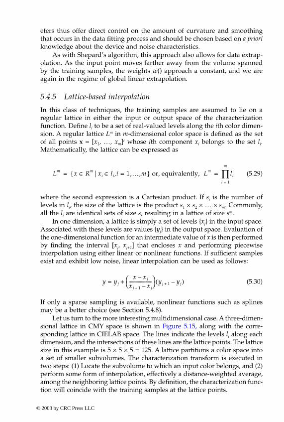
Let us turn to the more interesting multidimensional case. A three-dimen-sional lattice in CMY space is shown in Figure 5.15, along with the corre-sponding lattice in CIELAB space. The lines indicate the levels li along eachdimension, and the intersections of these lines are the lattice points. The latticesize in this example is 5 × 5 × 5 = 125. A lattice partitions a color space intoa set of smaller subvolumes. The characterization transform is executed intwo steps: (1) Locate the subvolume to which an input color belongs, and (2)perform some form of interpolation, effectively a distance-weighted average,among the neighboring lattice points. By definition, the characterization func-tion will coincide with the training samples at the lattice points.
Lm x Rm∈ |xi li,i∈ 1,…,m={ } or, equivalently, Lm li
i 1=
m
∏= =
y yj=x xj–
xj 1+ xj–--------------------
yj 1+ yj–( )+
-ColorBook Page 301 Wednesday, November 13, 2002 10:55 AM
© 2003 by CRC Press LLC
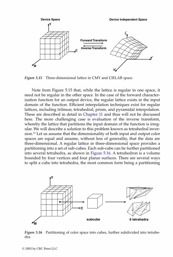
302 Digital Color Imaging Handbook
Note from Figure 5.15 that, while the lattice is regular in one space, itneed not be regular in the other space. In the case of the forward character-ization function for an output device, the regular lattice exists in the inputdomain of the function. Efficient interpolation techniques exist for regularlattices, including trilinear, tetrahedral, prism, and pyramidal interpolation.These are described in detail in Chapter 11 and thus will not be discussedhere. The more challenging case is evaluation of the inverse transform,whereby the lattice that partitions the input domain of the function is irreg-ular. We will describe a solution to this problem known as tetrahedral inver-sion.13 Let us assume that the dimensionality of both input and output colorspaces are equal and assume, without less of generality, that the data arethree-dimensional. A regular lattice in three-dimensional space provides apartitioning into a set of sub-cubes. Each sub-cube can be further partitionedinto several tetrahedra, as shown in Figure 5.16. A tetrahedron is a volumebounded by four vertices and four planar surfaces. There are several waysto split a cube into tetrahedra, the most common form being a partitioning
L
a
b
*
*
*
Device Independent Space
Forward Transform
Inverse Transform
Device Space
Y
C
M
Figure 5.15 Three-dimensional lattice in CMY and CIELAB space.
subcube 6 tetrahedra
Y
C
M
Figure 5.16 Partitioning of color space into cubes, further subdivided into tetrahe-dra.
-ColorBook Page 302 Wednesday, November 13, 2002 10:55 AM
© 2003 by CRC Press LLC
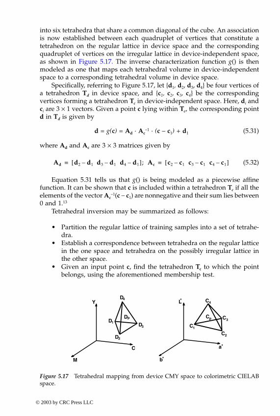
Chapter five: Device characterization 303
into six tetrahedra that share a common diagonal of the cube. An associationis now established between each quadruplet of vertices that constitute atetrahedron on the regular lattice in device space and the correspondingquadruplet of vertices on the irregular lattice in device-independent space,as shown in Figure 5.17. The inverse characterization function g() is thenmodeled as one that maps each tetrahedral volume in device-independentspace to a corresponding tetrahedral volume in device space.
Specifically, referring to Figure 5.17, let {d1, d2, d3, d4} be four vertices ofa tetrahedron Td in device space, and {c1, c2, c3, c4} be the correspondingvertices forming a tetrahedron Tc in device-independent space. Here, di andci are 3 × 1 vectors. Given a point c lying within Tc, the corresponding pointd in Td is given by
d = g(c) = Ad · Ac–1 · (c – c1) + d1 (5.31)
where Ad and Ac are 3 × 3 matrices given by
(5.32)
Equation 5.31 tells us that g() is being modeled as a piecewise affinefunction. It can be shown that c is included within a tetrahedron Tc if all theelements of the vector Ac
–1(c – c1) are nonnegative and their sum lies between0 and 1.13
Tetrahedral inversion may be summarized as follows:
• Partition the regular lattice of training samples into a set of tetrahe-dra.
• Establish a correspondence between tetrahedra on the regular latticein the one space and tetrahedra on the possibly irregular lattice inthe other space.
• Given an input point c, find the tetrahedron Tc to which the pointbelongs, using the aforementioned membership test.
Y
C
M
D1
D2
D4
D3
Dp
L
a
b
*
*
*
C1
C4
Cp C3
C2
Figure 5.17 Tetrahedral mapping from device CMY space to colorimetric CIELABspace.
Ad d2 d1– d3 d1– d4 d1–[ ]; Ac c2 c1– c3 c1– c4 c1–[ ]= =
-ColorBook Page 303 Wednesday, November 13, 2002 10:55 AM
© 2003 by CRC Press LLC
304 Digital Color Imaging Handbook
• Use Equations 5.31 and 5.32 to evaluate the characterization functiond = g(c).
Because tetrahedral inversion requires membership in a tetrahedron, it doesnot allow extrapolation to points c that lie outside the lattice defined by thetraining samples. Hence, such points must first be mapped to the latticevolume before carrying out the inversion algorithm. Also, it is worth notingthat tetrahedral interpolation on a regular lattice can be implemented witha highly simplified form of Equation 5.31. These equations will be includedin the chapter on efficient color transformations.
In the context of deriving a characterization function, regular lattices oftraining data can occur only for the case of output devices, as the patchesin the color target can be designed to lie on a regular lattice in device space.With input device characterization, neither the captured device values northe measured device-independent values of the color target can be guaran-teed to lie on a regular lattice.
5.4.6 Sequential interpolation
A primary advantage of a regular lattice is that it facilitates simple interpo-lation techniques. However, it limits the freedom in the placement of controlpoints in multidimensional color space. Referring to Figure 5.12, one wouldexpect considerable curvature of the characterization function in certainregions within the device gamut, while large regions outside the gamutwould never be used for interpolation calculations. It would be desirable,therefore, to finely sample regions within the gamut, and coarsely sampleregions far away from the gamut. As shown in the figure, the regular latticedoes not permit this. A simple extension of regular lattice interpolation,which we term sequential interpolation (SI), brings additional flexibility at amodest increase in computational cost.
In general terms, SI can be thought of as a two-stage interpolation pro-cess. Consider a decomposition of the space Rm into two subspaces of dimen-sions p and q, i.e., Rm = Rp × Rq, m = p + q. The m-dimensional lattice Lm canalso be decomposed into two sub-lattices Lp and Lq. Let s be the size of Lq.We can think of Lm as being a family of s p-dimensional lattices. In a conven-tional regular lattice each p-dimensional lattice is identical, and we have Lm
= Lp × Lq. In sequential interpolation, we let the p-dimensional lattice structurevary as a function of the remaining q dimensions.
To crystallize this concept, consider the three-dimensional lattice in Figure5.18 used to implement a characterization function from device RGB toCIELAB. This lattice can be conceived as a family of two-dimensional RGlattices, corresponding to different levels of the third-dimension B. In Figure5.18a, the RG lattices are identical as a function of B, which corresponds to aregular lattice in RGB space. In this case, interpolation of an input RGB pointis accomplished by selecting a subset of the eight vertices V1, . . ., V8 thatenclose the point and performing a weighted average of the output values at
-ColorBook Page 304 Wednesday, November 13, 2002 10:55 AM
© 2003 by CRC Press LLC
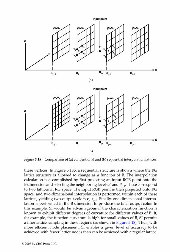
Chapter five: Device characterization 305
these vertices. In Figure 5.18b, a sequential structure is shown where the RGlattice structure is allowed to change as a function of B. The interpolationcalculation is accomplished by first projecting an input RGB point onto theB dimension and selecting the neighboring levels Bj and Bj+1. These correspondto two lattices in RG space. The input RGB point is then projected onto RGspace, and two-dimensional interpolation is performed within each of theselattices, yielding two output colors cj, cj+1. Finally, one-dimensional interpo-lation is performed in the B dimension to produce the final output color. Inthis example, SI would be advantageous if the characterization function isknown to exhibit different degrees of curvature for different values of B. If,for example, the function curvature is high for small values of B, SI permitsa finer lattice sampling in these regions (as shown in Figure 5.18). Thus, withmore efficient node placement, SI enables a given level of accuracy to beachieved with fewer lattice nodes than can be achieved with a regular lattice.
input point
R
G
B
(5x5)(5x5) (5x5) (5x5)
V
V
V
VV
V
V
V1
2
34
5
6
7
8
B B B B Bjj-1 j+1 j+2in
input point
R
G
B
(5x5)(7x7) (4x4) (3x3)
V
V
V
VV
V
V
V1
2
34
5
6
7
8
B B B B Bjj-1 j+1 j+2in
Figure 5.18 Comparison of (a) conventional and (b) sequential interpolation lattices.
(a)
(b)
-ColorBook Page 305 Wednesday, November 13, 2002 10:55 AM
© 2003 by CRC Press LLC
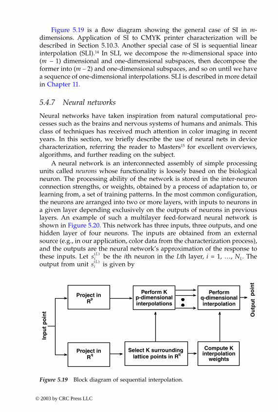
306 Digital Color Imaging Handbook
Figure 5.19 is a flow diagram showing the general case of SI in m-dimensions. Application of SI to CMYK printer characterization will bedescribed in Section 5.10.3. Another special case of SI is sequential linearinterpolation (SLI).14 In SLI, we decompose the m-dimensional space into(m – 1) dimensional and one-dimensional subspaces, then decompose theformer into (m – 2) and one-dimensional subspaces, and so on until we havea sequence of one-dimensional interpolations. SLI is described in more detailin Chapter 11.
5.4.7 Neural networks
Neural networks have taken inspiration from natural computational pro-cesses such as the brains and nervous systems of humans and animals. Thisclass of techniques has received much attention in color imaging in recentyears. In this section, we briefly describe the use of neural nets in devicecharacterization, referring the reader to Masters15 for excellent overviews,algorithms, and further reading on the subject.
A neural network is an interconnected assembly of simple processingunits called neurons whose functionality is loosely based on the biologicalneuron. The processing ability of the network is stored in the inter-neuronconnection strengths, or weights, obtained by a process of adaptation to, orlearning from, a set of training patterns. In the most common configuration,the neurons are arranged into two or more layers, with inputs to neurons ina given layer depending exclusively on the outputs of neurons in previouslayers. An example of such a multilayer feed-forward neural network isshown in Figure 5.20. This network has three inputs, three outputs, and onehidden layer of four neurons. The inputs are obtained from an externalsource (e.g., in our application, color data from the characterization process),and the outputs are the neural network’s approximation of the response tothese inputs. Let be the ith neuron in the Lth layer, i = 1, …, NL. Theoutput from unit is given by
Inp
ut
po
int
Project inRp
Perform Kp-dimensionalinterpolations
Performq-dimensionalinterpolation
Ou
tpu
t p
oin
t
Select K surroundinglattice points in Rq
Compute Kinterpolation
weights
Project inRq
Figure 5.19 Block diagram of sequential interpolation.
siL( )
siL( )
-ColorBook Page 306 Wednesday, November 13, 2002 10:55 AM
© 2003 by CRC Press LLC
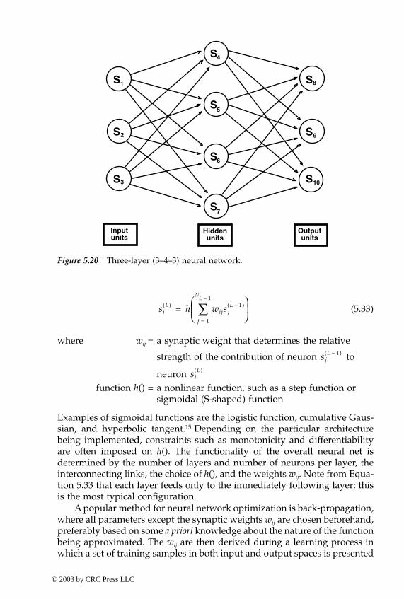
Chapter five: Device characterization 307
(5.33)
where wij = a synaptic weight that determines the relative
strength of the contribution of neuron to
neuron function h() = a nonlinear function, such as a step function or
sigmoidal (S-shaped) function
Examples of sigmoidal functions are the logistic function, cumulative Gaus-sian, and hyperbolic tangent.15 Depending on the particular architecturebeing implemented, constraints such as monotonicity and differentiabilityare often imposed on h(). The functionality of the overall neural net isdetermined by the number of layers and number of neurons per layer, theinterconnecting links, the choice of h(), and the weights wij. Note from Equa-tion 5.33 that each layer feeds only to the immediately following layer; thisis the most typical configuration.
A popular method for neural network optimization is back-propagation,where all parameters except the synaptic weights wij are chosen beforehand,preferably based on some a priori knowledge about the nature of the functionbeing approximated. The wij are then derived during a learning process inwhich a set of training samples in both input and output spaces is presented
S
S
S
S
S
S
S
S
S
S
Inputunits
Hiddenunits
Outputunits
1
2
3
4
5
6
7
8
9
10
Figure 5.20 Three-layer (3–4–3) neural network.
siL( ) h wijs j
L 1–( )
j 1=
L 1–N
∑
=
sjL 1–( )
siL( )
-ColorBook Page 307 Wednesday, November 13, 2002 10:55 AM
© 2003 by CRC Press LLC
308 Digital Color Imaging Handbook
to the network. An error metric such as the mean squared error in Equation5.12 is minimized at the training samples with respect to wij. Because theoverall neural network is a complex nonlinear function of wij, iterative errorminimization approaches are called for. An example is the gradient descentalgorithm, where a weight at iteration k is given by
(5.34)
Here, E is the error metric being minimized, and R is a parameter known asthe learning rate. The iteration continues until some convergence criterionis met with respect to the magnitude or the rate of change of E. The parameterR dictates the speed and stability of convergence. A major shortcoming ofthe gradient descent algorithm is that convergence is often unacceptablyslow. An alternative search technique favored for significantly faster conver-gence is the conjugate gradient algorithm. As with all iterative algorithms,rate of convergence also depends on the choice of initial estimates, i.e., .Linear regression can be used to generate good initial estimates. Details aregiven in the book by Masters.15
The application to color characterization should be evident. A neuralnetwork can be used to approximate either the forward or inverse charac-terization functions. The training samples are the device-dependent anddevice-independent colors {ci, di} obtained in the characterization process.After the neural net is trained, arbitrary color inputs can now be processedthrough the network. The architecture of the network is chosen based on theexpected complexity of the characterization function. As with polynomials,increased complexity can result in a better fit up to a certain point, beyondwhich the network will begin to track the noise in the data.
Typically, the iterative training can be a highly computationally intensiveprocess. Fortunately, this is not a major concern, as this step is carried outoffline. Neural networks are also usually too computationally intensive forreal-time processing of image pixels. They can, however, be approximatedby multidimensional LUTs, which are more computationally efficient.
5.4.8 Spline fitting
Spline interpolation constitutes a rich and flexible framework for approxi-mating free-form shapes. One-dimensional splines can be used very effec-tively for the calibration step, whereas the multidimensional versions areapplicable for characterization. The most common spline functions comprisea set of piecewise polynomial functions defined over a partition of segmentsin the input space, as shown for the one-dimensional case in Figure 5.21.The behavior of the spline is dictated by control points, known as knots, atthe segment boundaries. The parameters of the polynomials are determinedso that the function passes through all the knots while maintaining certaindegrees of continuity across the segment boundaries.
wijk( )
wijk( ) wij
k 1–( ) R δEδwij----------
–=
wij0( )
-ColorBook Page 308 Wednesday, November 13, 2002 10:55 AM
© 2003 by CRC Press LLC
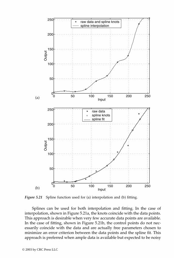
Chapter five: Device characterization 309
Splines can be used for both interpolation and fitting. In the case ofinterpolation, shown in Figure 5.21a, the knots coincide with the data points.This approach is desirable when very few accurate data points are available.In the case of fitting, shown in Figure 5.21b, the control points do not nec-essarily coincide with the data and are actually free parameters chosen tominimize an error criterion between the data points and the spline fit. Thisapproach is preferred when ample data is available but expected to be noisy
0 50 100 150 200 2500
50
100
150
200
250
Input
Out
put
raw data and spline knotsspline interpolation___
0 50 100 150 200 2500
50
100
150
200
250
Input
Out
put
raw dataspline knotsspline fit___°
Figure 5.21 Spline function used for (a) interpolation and (b) fitting.
(a)
(b)
-ColorBook Page 309 Wednesday, November 13, 2002 10:55 AM
© 2003 by CRC Press LLC
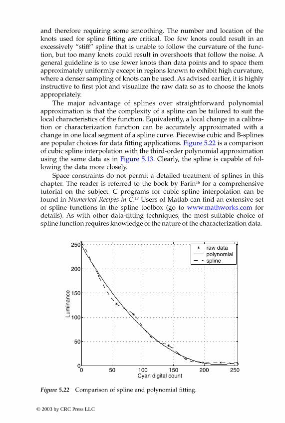
310 Digital Color Imaging Handbook
and therefore requiring some smoothing. The number and location of theknots used for spline fitting are critical. Too few knots could result in anexcessively “stiff” spline that is unable to follow the curvature of the func-tion, but too many knots could result in overshoots that follow the noise. Ageneral guideline is to use fewer knots than data points and to space themapproximately uniformly except in regions known to exhibit high curvature,where a denser sampling of knots can be used. As advised earlier, it is highlyinstructive to first plot and visualize the raw data so as to choose the knotsappropriately.
The major advantage of splines over straightforward polynomialapproximation is that the complexity of a spline can be tailored to suit thelocal characteristics of the function. Equivalently, a local change in a calibra-tion or characterization function can be accurately approximated with achange in one local segment of a spline curve. Piecewise cubic and B-splinesare popular choices for data fitting applications. Figure 5.22 is a comparisonof cubic spline interpolation with the third-order polynomial approximationusing the same data as in Figure 5.13. Clearly, the spline is capable of fol-lowing the data more closely.
Space constraints do not permit a detailed treatment of splines in thischapter. The reader is referred to the book by Farin16 for a comprehensivetutorial on the subject. C programs for cubic spline interpolation can befound in Numerical Recipes in C.17 Users of Matlab can find an extensive setof spline functions in the spline toolbox (go to www.mathworks.com fordetails). As with other data-fitting techniques, the most suitable choice ofspline function requires knowledge of the nature of the characterization data.
0 50 100 150 200 2500
50
100
150
200
250
Cyan digital count
Lum
inan
ce
raw datapolynomialspline
Figure 5.22 Comparison of spline and polynomial fitting.
-ColorBook Page 310 Wednesday, November 13, 2002 10:55 AM
© 2003 by CRC Press LLC
Chapter five: Device characterization 311
5.5 Metrics for evaluating device characterizationMany of the mathematical techniques described in the previous sectionminimize quantitative error metrics. The resulting error from the fitting orinterpolation is one indicator of the overall accuracy of characterization.However, this information is not sufficient, for several reasons:
1. The error is available only for the training samples. 2. The error is not always calculated in a visually meaningful color
space.3. Noise and other imperfections that can occur with multiple uses of
the device are implicitly ignored.
To address the first concern, the notion of evaluating the characterizationwith independent test targets was introduced in Section 5.2. To address thesecond issue, evaluation of errors with visually relevant metrics is stronglyrecommended. While color difference formulae are described in detail in anearlier chapter, two of them, ∆ and ∆ are restated here, as they areused extensively in this chapter. Given two CIELAB colors, and their com-ponent-wise differences, ∆L*, ∆a*, ∆b* (equivalently, ∆L*, ∆C*, ∆H*), the ∆color difference formula is simply the Euclidean distance between the twopoints in CIELAB space,
(5.35)
It is important to bear in mind that ∆H* is not a component-wise hue differ-ence but rather is given by
(5.36)
The ∆ formula is an extension of ∆ that applies different weights tothe various components as follows:
(5.37)
where SL = 1SC = 1 + 0.045 C*SH = 1 + 0.015 C*
The parameters kL, kC, and kH account for the effect of viewing conditions.Under a set of nominal viewing conditions, these parameters are set to 1,
Eab* E94
*
Eab*
∆Eab* ∆L*( )2 ∆a*( )2 ∆b*( )2
+ + ∆L*( )2 ∆C*( )2 ∆H*( )2+ += =
∆H* ∆Eab*( )
2∆L*( )2 ∆C*( )2––=
E94* Eab
*
∆E*94
∆L*
kLSL-----------
2 ∆C*
kCSC-----------
2 ∆H*
kHSH------------
2
+ +=
-ColorBook Page 311 Wednesday, November 13, 2002 10:55 AM
© 2003 by CRC Press LLC
312 Digital Color Imaging Handbook
and the overall effect is dictated solely by SC and SH, which reduce theperceived color difference as chroma increases.
Another metric used widely in the textile industry is the CMC colordifference formula. This formula is similar in form to the ∆ equation andhas parameters tailored for perceptibility vs. acceptability of color differ-ences. Finally, an extension of the ∆ formula has been recently developed,known as the CIEDE2000 metric.18 This metric accounts for interactionsbetween the C* and H* terms and is expected to be adopted as an industrystandard until further developments arise. The reader is referred to Chapter 1for details.
The next question to consider is what error statistics to report. Commonaggregate statistics cited in the literature are the mean, standard deviation,minimum, and maximum of the ∆Es for a set of test samples. Often, acumulative statistic such as the 95th percentile of ∆E values (i.e., the valuebelow which 95% of the ∆E values in the test data lie) is calculated. For acomplete statistical description, histograms of ∆E can also be reported.
Having chosen an error metric, how does one determine that the char-acterization error is satisfactorily small? First, recall that characterizationaccuracy is limited by the inherent stability and uniformity of a given device.If the errors are close to this lower bound, we know that we cannot do muchbetter for the given device. In the following sections, we will provide thereader with some idea of the characterization accuracy achievable by state-of-the-art techniques. It must be kept in mind, however, that “satisfactoryaccuracy” depends strongly on the application and the needs and expecta-tions of a user. A graphic arts color proofing application will likely placestringent demands on color accuracy, while inexpensive consumer productswill typically play in a market with wider color tolerances.
Another aspect that further confounds evaluation of color accuracy isthat the end user ultimately views not test targets with color patches butimages with complex color and spatial characteristics. Unfortunately, quan-titative analysis of patches is not always a reliable indicator of perceivedcolor quality in complex images. (The latter is a subject of active research.19)The reader is thus advised to exercise appropriate caution when interpretingindividual results or those cited in the literature, and to always augmentquantitative evaluation of color accuracy with a qualitative evaluationinvolving images and individuals that represent the intended market andapplication.
A special class of error metrics for input devices evaluates how accu-rately the information recorded by the input device can be transformed intothe signals sensed by the human visual system for input stimuli with givenspectral statistics. Such error metrics do not directly evaluate the accuracyof a characterization but rather the ability of the device to act as a visualcolorimeter. Hence, these metrics are relevant for filter design optimizationand can also suggest the most appropriate characterization technique for agiven input device. The reader is referred to papers by Sharma et al.20 andQuan et al.21 for further details.
E94*
E94*
-ColorBook Page 312 Wednesday, November 13, 2002 10:55 AM
© 2003 by CRC Press LLC
Chapter five: Device characterization 313
5.6 ScannersAll scanners employ one of two primary types of sensing technology. Drumscanners use photomultiplier tubes (PMTs), whereas the less expensive flat-bed scanners employ charge-coupled devices (CCDs). Both of these technol-ogies sense and convert light input into analog voltage. Drum scannersconsist of a removable transparent cylinder on which a print, which is reflec-tive, transparent, or a photographic negative, can be mounted. A light sourceilluminates the image in a single pass as the drum spins at a high speed.The light reflected off or transmitted through the print is passed throughred, green, and blue filters then sent through the PMTs, which relay voltagesproportional to the input light intensity. The PMT is extremely sensitive, thusproviding drum scanners a large dynamic range. The drum scanners usedin offset printing applications contain built-in computers that are capable ofdirect conversion of the RGB scan to CMYK output and are used to generatecolor separations at very high spatial resolution. A limitation of this scanningtechnology is that the original must be flexible so that it can physically bemounted on the drum.
All flatbed scanners utilize CCD technology, which is simpler, morestable, and less costly than PMT technology. These scanners have widelyvarying sensitivity and resolution and, at the highest end, approach theperformance of drum scanners. Transparent or reflective prints are placedon a glass platen and evenly illuminated from above the glass for transpar-encies, and from beneath for reflective. As the light source moves across theimage, individual lines of the image are sensed by a CCD array, which relaysvoltages that are proportional to the input light intensity. An integratingcavity is usually employed to focus light from the scanner illuminant ontothe print. An undesirable outcome of this is that light reflected from a givenspatial location on the print can be captured by the cavity and returned tothe print at neighboring locations. Hence, the scanner measurement at a pixeldepends not only on the reflectance at that pixel but also on the reflectancesof neighboring pixels. A model and correction algorithm for this so-calledintegrating cavity effect is given by Knox.22
Following the sensing step, an analog-to-digital (A/D) converter is usedto quantize the analog voltage signal to a digital signal represented bybetween 8 and 16 bits per each of R, G, B channels. These raw digital valuesare usually linear with respect to the luminance of the stimulus beingscanned. Additional image acquisition software often allows the raw datato be processed through tone reproduction curves so that a power-law (orgamma) relationship exists between digital value and luminance. This oper-ation is carried out before the A/D conversion. One reason for doing this isthat quantization of nonlinear gamma-corrected signals is less visually dis-turbing than quantization of data that is linear in luminance. (This is dis-cussed in more detail in the section on display characterization.) A secondreason is to prepare the scanned data for direct display on a CRT, whichexhibits approximately a square law (gamma = 2) relationship.
-ColorBook Page 313 Wednesday, November 13, 2002 10:55 AM
© 2003 by CRC Press LLC
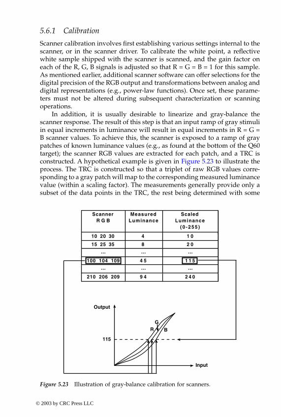
314 Digital Color Imaging Handbook
5.6.1 Calibration
Scanner calibration involves first establishing various settings internal to thescanner, or in the scanner driver. To calibrate the white point, a reflectivewhite sample shipped with the scanner is scanned, and the gain factor oneach of the R, G, B signals is adjusted so that R = G = B = 1 for this sample.As mentioned earlier, additional scanner software can offer selections for thedigital precision of the RGB output and transformations between analog anddigital representations (e.g., power-law functions). Once set, these parame-ters must not be altered during subsequent characterization or scanningoperations.
In addition, it is usually desirable to linearize and gray-balance thescanner response. The result of this step is that an input ramp of gray stimuliin equal increments in luminance will result in equal increments in R = G =B scanner values. To achieve this, the scanner is exposed to a ramp of graypatches of known luminance values (e.g., as found at the bottom of the Q60target); the scanner RGB values are extracted for each patch, and a TRC isconstructed. A hypothetical example is given in Figure 5.23 to illustrate theprocess. The TRC is constructed so that a triplet of raw RGB values corre-sponding to a gray patch will map to the corresponding measured luminancevalue (within a scaling factor). The measurements generally provide only asubset of the data points in the TRC, the rest being determined with some
ScannerR G B
MeasuredLuminance
ScaledLuminance
( 0 - 2 5 5 )
10 20 30 4 1 0
15 25 35 8 2 0… … …
100 104 109 4 5 1 1 5… … …
210 206 209 9 4 2 4 0
Input
Output
115
RG
B
Figure 5.23 Illustration of gray-balance calibration for scanners.
-ColorBook Page 314 Wednesday, November 13, 2002 10:55 AM
© 2003 by CRC Press LLC
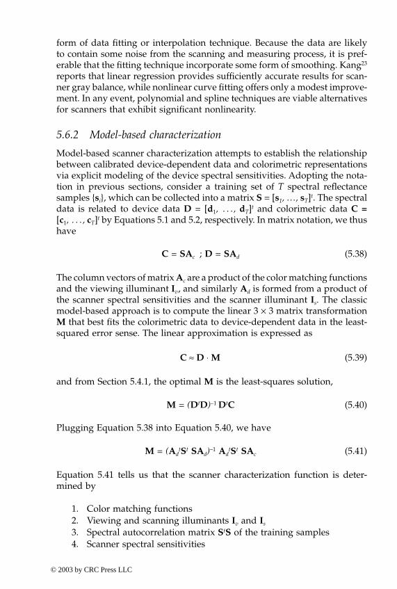
Chapter five: Device characterization 315
form of data fitting or interpolation technique. Because the data are likelyto contain some noise from the scanning and measuring process, it is pref-erable that the fitting technique incorporate some form of smoothing. Kang23
reports that linear regression provides sufficiently accurate results for scan-ner gray balance, while nonlinear curve fitting offers only a modest improve-ment. In any event, polynomial and spline techniques are viable alternativesfor scanners that exhibit significant nonlinearity.
5.6.2 Model-based characterization
Model-based scanner characterization attempts to establish the relationshipbetween calibrated device-dependent data and colorimetric representationsvia explicit modeling of the device spectral sensitivities. Adopting the nota-tion in previous sections, consider a training set of T spectral reflectancesamples {si}, which can be collected into a matrix S = [s1, …, sT]t. The spectraldata is related to device data D = [d1, . . . , dT]t and colorimetric data C =[c1, . . . , cT]t by Equations 5.1 and 5.2, respectively. In matrix notation, we thushave
C = SAc ; D = SAd (5.38)
The column vectors of matrix Ac are a product of the color matching functionsand the viewing illuminant Iv, and similarly Ad is formed from a product ofthe scanner spectral sensitivities and the scanner illuminant Is. The classicmodel-based approach is to compute the linear 3 × 3 matrix transformationM that best fits the colorimetric data to device-dependent data in the least-squared error sense. The linear approximation is expressed as
(5.39)
and from Section 5.4.1, the optimal M is the least-squares solution,
M = (DtD)–1 DtC (5.40)
Plugging Equation 5.38 into Equation 5.40, we have
M = (AdtSt SAd)–1 Ad
tSt SAc (5.41)
Equation 5.41 tells us that the scanner characterization function is deter-mined by
1. Color matching functions2. Viewing and scanning illuminants Iv and Is
3. Spectral autocorrelation matrix StS of the training samples4. Scanner spectral sensitivities
C D M⋅≈
-ColorBook Page 315 Wednesday, November 13, 2002 10:55 AM
© 2003 by CRC Press LLC
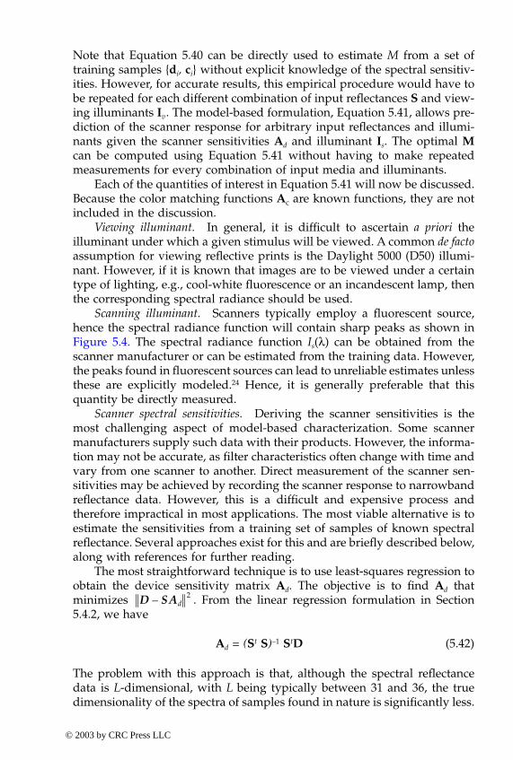
316 Digital Color Imaging Handbook
Note that Equation 5.40 can be directly used to estimate M from a set oftraining samples {di, ci} without explicit knowledge of the spectral sensitiv-ities. However, for accurate results, this empirical procedure would have tobe repeated for each different combination of input reflectances S and view-ing illuminants Iv. The model-based formulation, Equation 5.41, allows pre-diction of the scanner response for arbitrary input reflectances and illumi-nants given the scanner sensitivities Ad and illuminant Is. The optimal Mcan be computed using Equation 5.41 without having to make repeatedmeasurements for every combination of input media and illuminants.
Each of the quantities of interest in Equation 5.41 will now be discussed.Because the color matching functions Ac are known functions, they are notincluded in the discussion.
Viewing illuminant. In general, it is difficult to ascertain a priori theilluminant under which a given stimulus will be viewed. A common de factoassumption for viewing reflective prints is the Daylight 5000 (D50) illumi-nant. However, if it is known that images are to be viewed under a certaintype of lighting, e.g., cool-white fluorescence or an incandescent lamp, thenthe corresponding spectral radiance should be used.
Scanning illuminant. Scanners typically employ a fluorescent source,hence the spectral radiance function will contain sharp peaks as shown inFigure 5.4. The spectral radiance function Is(λ) can be obtained from thescanner manufacturer or can be estimated from the training data. However,the peaks found in fluorescent sources can lead to unreliable estimates unlessthese are explicitly modeled.24 Hence, it is generally preferable that thisquantity be directly measured.
Scanner spectral sensitivities. Deriving the scanner sensitivities is themost challenging aspect of model-based characterization. Some scannermanufacturers supply such data with their products. However, the informa-tion may not be accurate, as filter characteristics often change with time andvary from one scanner to another. Direct measurement of the scanner sen-sitivities may be achieved by recording the scanner response to narrowbandreflectance data. However, this is a difficult and expensive process andtherefore impractical in most applications. The most viable alternative is toestimate the sensitivities from a training set of samples of known spectralreflectance. Several approaches exist for this and are briefly described below,along with references for further reading.
The most straightforward technique is to use least-squares regression toobtain the device sensitivity matrix Ad. The objective is to find Ad thatminimizes . From the linear regression formulation in Section5.4.2, we have
Ad = (St S)–1 StD (5.42)
The problem with this approach is that, although the spectral reflectancedata is L-dimensional, with L being typically between 31 and 36, the truedimensionality of the spectra of samples found in nature is significantly less.
D SAd– 2
-ColorBook Page 316 Wednesday, November 13, 2002 10:55 AM
© 2003 by CRC Press LLC
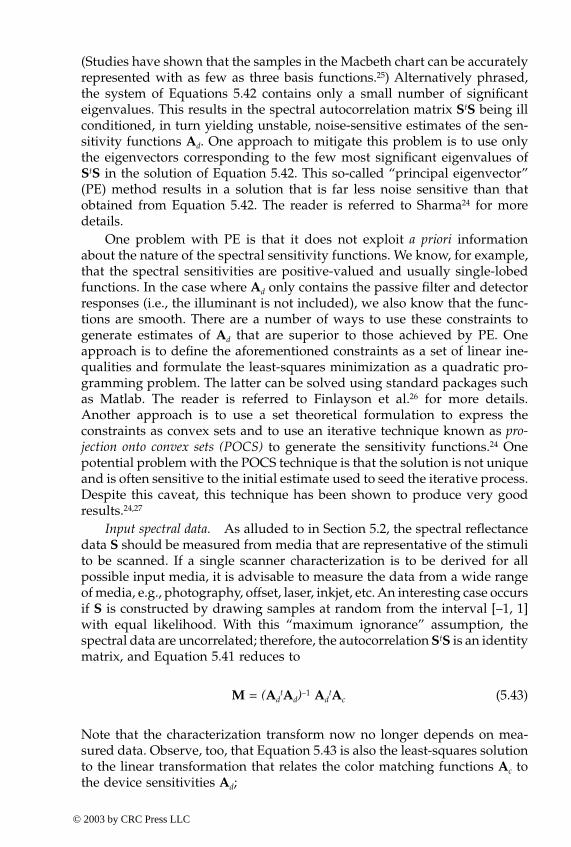
Chapter five: Device characterization 317
(Studies have shown that the samples in the Macbeth chart can be accuratelyrepresented with as few as three basis functions.25) Alternatively phrased,the system of Equations 5.42 contains only a small number of significanteigenvalues. This results in the spectral autocorrelation matrix StS being illconditioned, in turn yielding unstable, noise-sensitive estimates of the sen-sitivity functions Ad. One approach to mitigate this problem is to use onlythe eigenvectors corresponding to the few most significant eigenvalues ofStS in the solution of Equation 5.42. This so-called “principal eigenvector”(PE) method results in a solution that is far less noise sensitive than thatobtained from Equation 5.42. The reader is referred to Sharma24 for moredetails.
One problem with PE is that it does not exploit a priori informationabout the nature of the spectral sensitivity functions. We know, for example,that the spectral sensitivities are positive-valued and usually single-lobedfunctions. In the case where Ad only contains the passive filter and detectorresponses (i.e., the illuminant is not included), we also know that the func-tions are smooth. There are a number of ways to use these constraints togenerate estimates of Ad that are superior to those achieved by PE. Oneapproach is to define the aforementioned constraints as a set of linear ine-qualities and formulate the least-squares minimization as a quadratic pro-gramming problem. The latter can be solved using standard packages suchas Matlab. The reader is referred to Finlayson et al.26 for more details.Another approach is to use a set theoretical formulation to express theconstraints as convex sets and to use an iterative technique known as pro-jection onto convex sets (POCS) to generate the sensitivity functions.24 Onepotential problem with the POCS technique is that the solution is not uniqueand is often sensitive to the initial estimate used to seed the iterative process.Despite this caveat, this technique has been shown to produce very goodresults.24,27
Input spectral data. As alluded to in Section 5.2, the spectral reflectancedata S should be measured from media that are representative of the stimulito be scanned. If a single scanner characterization is to be derived for allpossible input media, it is advisable to measure the data from a wide rangeof media, e.g., photography, offset, laser, inkjet, etc. An interesting case occursif S is constructed by drawing samples at random from the interval [–1, 1]with equal likelihood. With this “maximum ignorance” assumption, thespectral data are uncorrelated; therefore, the autocorrelation StS is an identitymatrix, and Equation 5.41 reduces to
M = (AdtAd)–1 Ad
tAc (5.43)
Note that the characterization transform now no longer depends on mea-sured data. Observe, too, that Equation 5.43 is also the least-squares solutionto the linear transformation that relates the color matching functions Ac tothe device sensitivities Ad;
-ColorBook Page 317 Wednesday, November 13, 2002 10:55 AM
© 2003 by CRC Press LLC
318 Digital Color Imaging Handbook
Ac ≈ AdM (5.44)
Comparing Equations 5.39 and 5.44, we see that the optimal linear trans-form that maps the color matching functions to the scanner sensitivities isthe same as the transform that optimally maps scanner RGB to XYZ underthe maximum ignorance assumption. As a corollary, if the scanner is perfectlycolorimetric, then Equations 5.39 and 5.44 become equalities, and the matrixthat relates the color matching functions to scanner sensitivities is preciselythe matrix that maps scanner RGB to XYZ for all media and illuminants.
One problem with the maximum ignorance assumption is that it includesnegative values, which can never occur with physical spectra. Finlayson etal.28 show that a positivity constraint on the preceding formulation resultsin the correlation StS being a constant (but not identity) matrix, which resultsin a more accurate estimate of M.
Another class of model-based techniques, somewhat distinct from thepreceding framework, derives scanner characterization for a specificmedium by first characterizing the medium itself and using models for boththe medium and scanner to generate the characterization. The additionalstep of modeling the medium imposes physically based constraints on thepossible spectra S and can lend further insight into the interaction betweenthe medium and the scanner. Furthermore, a priori modeling of the inputmedium may simplify the in situ color measurement process. Berns andShyu29 postulate that scanner filters are designed to align closely with thepeaks of the spectral absorptivity functions of typical photographic dyes.The relationship between scanner RGB and C, M, Y dye concentrations isthus modeled by simple polynomial functions. The Beer–Bouguer andKubelka–Munk theories (discussed in Section 5.10.2) are then used to relatedye concentrations to reflectance spectra for photographic media. Sharma30
models the color formation process on photographic media using theBeer–Bouguer model. From this model, and using a small number of mea-surements on the actual sample being scanned, the set Smedium of all reflectancespectra reproducible by the given medium is estimated. For a given scannerRGB triplet, the set Sscanner of all reflectance spectra that can generate thistriplet is derived with knowledge of the scanner spectral sensitivities, Ad.The actual input reflectance spectrum lies in the intersection and is derived using POCS. Note that both these approaches generate spec-tral characterizations, i.e., mappings from scanner RGB to spectral reflec-tance. From this, colorimetric characterizations can readily be generated forarbitrary viewing illuminants.
5.6.3 Empirical characterization
Empirical approaches derive the characterization function by correlatingmeasured CIE data from a target such as the Q60 to scanned RGB datafrom the target. Most of the data-fitting techniques described in Section 5.4can be used (with the exception of lattice-based approaches, as scanner
Smedium Sscanner∩
-ColorBook Page 318 Wednesday, November 13, 2002 10:55 AM
© 2003 by CRC Press LLC
Chapter five: Device characterization 319
characterization data cannot be designed to lie on a regular grid). Kang23
describes the use of polynomial regression to fit gray-balanced RGB data toCIEXYZ measurements. He compares 3 × 3, 3 × 6, 3 × 9, 3 × 11, and 3 × 14polynomial matrices derived using least-squares regression as described inSection 5.4.3. Several targets, including the MacBeth ColorChecker andKodak Q60, are used. The paper concludes that a 3 × 6 polynomial offersacceptable accuracy and that increasing the order of the polynomial mayimprove the fit to training data but may worsen the performance on inde-pendent test data. This is because, as noted in Section 5.4, higher-orderapproximations begin to track the noise in the data. The paper also exploresmedia dependence and concludes that the optimal 3 × 3 matrix does notvary considerably across media, whereas the optimal polynomial transformis indeed media dependent and will generally offer greater accuracy for anygiven medium.
Kang and Anderson31 describe the use of neural networks for scannercharacterization. They use a 3–4–3 network, trained by cascaded feed-for-ward correlation. A cumulative Gaussian function is used for the nonlinear-ity at each unit in the network (see Section 5.4.7). In comparison with poly-nomial regression, the neural network reports superior fits to training databut inferior performance for independent test data. Furthermore, the neuralnetwork is reported as being fairly sensitive to the choice of training data.Hence, while neural networks offer powerful capabilities for data fitting,much care must be exercised in their design and optimization to suit thenature of the particular device characteristics.
5.7 Digital still camerasDigital still cameras (DSCs) are becoming a common source for digital imag-ery. Their characterization is complicated by two factors.
1. The conditions under which images are captured are often uncon-trolled and can vary widely.
2. To compensate for this, DSC manufacturers build automatic image-processing algorithms into the devices to control and correct for flare,exposure, color balance, etc.
DSC characterization is probably unnecessary in most consumer applicationsand is called for only in specialized cases that require controlled, high-qualitycolor capture. In such cases, it is imperative that the automatic processingbe disabled or known to the extent that the raw DSC signals can be recoveredfrom the processed data.
A few precautions are in order for proper digital capture of calibrationand characterization targets. First, it must be ensured that the illuminationon the target is uniform. A viewing/illuminating geometry of 0/45 is rec-ommended so as to be consistent with the geometry of measurement devicesand typical visual viewing of hardcopy prints. Next, the lenses in most digital
-ColorBook Page 319 Wednesday, November 13, 2002 10:55 AM
© 2003 by CRC Press LLC
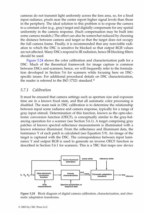
320 Digital Color Imaging Handbook
cameras do not transmit light uniformly across the lens area, so, for a fixedinput radiance, pixels near the center report higher signal levels than thosein the periphery. The ideal solution to this problem is to expose the camerato a constant color (e.g., gray) target and digitally compensate for any spatialuniformity in the camera response. (Such compensation may be built intosome camera models.) The effect can also be somewhat reduced by choosingthe distance between camera and target so that the target does not occupythe full camera frame. Finally, it is recommended that any nonvisible radi-ation to which the DSC is sensitive be blocked so that output RGB valuesare not affected. Many DSCs respond to IR radiation, hence IR blocking filtersshould be used.
Figure 5.24 shows the color calibration and characterization path for aDSC. Much of the theoretical framework for image capture is commonbetween DSCs and scanners; hence, we will frequently refer to the formula-tion developed in Section 5.6 for scanners while focusing here on DSC-specific issues. For additional procedural details on DSC characterization,the reader is referred to the ISO 17321 standard.32
5.7.1 Calibration
It must be ensured that camera settings such as aperture size and exposuretime are in a known fixed state, and that all automatic color processing isdisabled. The main task in DSC calibration is to determine the relationshipbetween input scene radiance and camera response, typically for a range ofgray input stimuli. Determination of this function, known as the opto-elec-tronic conversion function (OECF), is conceptually similar to the gray-bal-ancing operation for a scanner (see Section 5.6.1). A target comprising graypatches of known spectral reflectance measurements is illuminated with aknown reference illuminant. From the reflectance and illuminant data, theluminance Y of each patch is calculated (see Equation 5.9). An image of thetarget is captured with the DSC. The correspondence between input lumi-nance Y and output RGB is used to generate an inverse OECF function asdescribed in Section 5.6.1 for scanners. This is a TRC that maps raw device
Opto-electronicconversion
function
Scene illuminantestimation
scene white reference white
Graymeasurements
Spectral sensitivities orempirical data
Chromatic adaptationtransform
Inversecharacterization
XYZscene
XYZreference
Db
DgDr
Figure 5.24 Block diagram of digital camera calibration, characterization, and chro-matic adaptation transforms.
-ColorBook Page 320 Wednesday, November 13, 2002 10:55 AM
© 2003 by CRC Press LLC
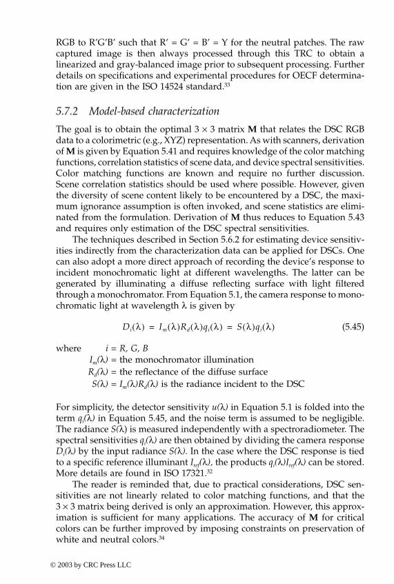
Chapter five: Device characterization 321
RGB to R’G’B’ such that R’ = G’ = B’ = Y for the neutral patches. The rawcaptured image is then always processed through this TRC to obtain alinearized and gray-balanced image prior to subsequent processing. Furtherdetails on specifications and experimental procedures for OECF determina-tion are given in the ISO 14524 standard.33
5.7.2 Model-based characterization
The goal is to obtain the optimal 3 × 3 matrix M that relates the DSC RGBdata to a colorimetric (e.g., XYZ) representation. As with scanners, derivationof M is given by Equation 5.41 and requires knowledge of the color matchingfunctions, correlation statistics of scene data, and device spectral sensitivities.Color matching functions are known and require no further discussion.Scene correlation statistics should be used where possible. However, giventhe diversity of scene content likely to be encountered by a DSC, the maxi-mum ignorance assumption is often invoked, and scene statistics are elimi-nated from the formulation. Derivation of M thus reduces to Equation 5.43and requires only estimation of the DSC spectral sensitivities.
The techniques described in Section 5.6.2 for estimating device sensitiv-ities indirectly from the characterization data can be applied for DSCs. Onecan also adopt a more direct approach of recording the device’s response toincident monochromatic light at different wavelengths. The latter can begenerated by illuminating a diffuse reflecting surface with light filteredthrough a monochromator. From Equation 5.1, the camera response to mono-chromatic light at wavelength λ is given by
(5.45)
where i = R, G, BIm(λ) = the monochromator illuminationRd(λ) = the reflectance of the diffuse surfaceS(λ) = Im(λ)Rd(λ) is the radiance incident to the DSC
For simplicity, the detector sensitivity u(λ) in Equation 5.1 is folded into theterm qi(λ) in Equation 5.45, and the noise term is assumed to be negligible.The radiance S(λ) is measured independently with a spectroradiometer. Thespectral sensitivities qi(λ) are then obtained by dividing the camera responseDi(λ) by the input radiance S(λ). In the case where the DSC response is tiedto a specific reference illuminant Iref(λ), the products qi(λ)Iref(λ) can be stored.More details are found in ISO 17321.32
The reader is reminded that, due to practical considerations, DSC sen-sitivities are not linearly related to color matching functions, and that the3 × 3 matrix being derived is only an approximation. However, this approx-imation is sufficient for many applications. The accuracy of M for criticalcolors can be further improved by imposing constraints on preservation ofwhite and neutral colors.34
Di λ( ) Im λ( )Rd λ( )qi λ( ) S λ( )qi λ( )= =
-ColorBook Page 321 Wednesday, November 13, 2002 10:55 AM
© 2003 by CRC Press LLC
322 Digital Color Imaging Handbook
5.7.3 Empirical characterization
As with scanners, empirical DSC characterization is accomplished by directlyrelating measured colorimetric data from a target and corresponding DSCRGB data obtained from a photographed image of the target. This approachis recommended in the case where the DSC spectral sensitivities areunknown, or when the target and illumination conditions used for charac-terization are expected to closely match those encountered during actualimage capture.
Hubel et al.35 compare several techniques for computing the optimal3 × 3 matrix M. One of these is a model-based approach that uses a whitepoint preserving maximum ignorance assumption, while the remaining tech-niques are empirical, using linear regression on training samples. They reportan extensive set of results for different illumination conditions. Average∆ECMC values range from approximately 2.5 to 6.5, depending on the tech-nique and illumination used. The model-based technique was often outper-formed by an empirical technique for a given medium and illuminant. How-ever, the model-based strategy, being oblivious to scene statistics, wasgenerally robust across different illumination conditions.
An empirically derived characterization need not be restricted to a lineartransformation. Hong et al.36 explore a polynomial technique to characterizea low-performance Canon PowerShot Pro70 camera for photographic input.A second-order polynomial was employed with 11 terms given by [Dr, Dg,Db, DrDg, DrDb, DgDb, Dr
2 , Dg2 , Db
2 , DrDgDb, 1]. The average characterizationerror for 264 training samples from an IT8.7/2 target was ∆ECMC(1:1) = 2.2. Asimilar technique37 was used to characterize a high-performance Agfa digitalStudioCam resulting in an average ∆ECMC(1:1) = 1.07. Note that these errorsare significantly lower than those reported by Hubel et al. This is not sur-prising, because polynomials can be expected to outperform linear approx-imations under a given set of controlled characterization conditions. Theother findings from these two studies are as follows:
• Correction for the OECF significantly improves overall characteriza-tion accuracy.
• For polynomial fitting, 40 to 60 training samples seem adequate;beyond this, there is little to be gained in characterization accuracy.
• The polynomial correction is highly dependent on the medium/col-orant combination.
• For a single medium/colorant combination, increasing the order ofthe polynomial up to 11 improves the characterization accuracy, withsome terms (notably DrDgDb and the constant term) being more im-portant than others. With the high-performance camera, a 3 × 11polynomial results in an average error of approximately 1 ∆ECMC(1:1).The low-performance camera results in ∆ECMC(1:1) = 2.2.
• For cross-media reproduction, increasing the order of the polyno-mials is not of significant benefit. Typical accuracy with a 3 × 11
-ColorBook Page 322 Wednesday, November 13, 2002 10:55 AM
© 2003 by CRC Press LLC
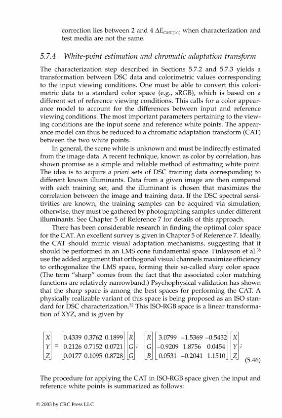
Chapter five: Device characterization 323
correction lies between 2 and 4 ∆ECMC(1:1) when characterization andtest media are not the same.
5.7.4 White-point estimation and chromatic adaptation transform
The characterization step described in Sections 5.7.2 and 5.7.3 yields atransformation between DSC data and colorimetric values correspondingto the input viewing conditions. One must be able to convert this colori-metric data to a standard color space (e.g., sRGB), which is based on adifferent set of reference viewing conditions. This calls for a color appear-ance model to account for the differences between input and referenceviewing conditions. The most important parameters pertaining to the view-ing conditions are the input scene and reference white points. The appear-ance model can thus be reduced to a chromatic adaptation transform (CAT)between the two white points.
In general, the scene white is unknown and must be indirectly estimatedfrom the image data. A recent technique, known as color by correlation, hasshown promise as a simple and reliable method of estimating white point.The idea is to acquire a priori sets of DSC training data corresponding todifferent known illuminants. Data from a given image are then comparedwith each training set, and the illuminant is chosen that maximizes thecorrelation between the image and training data. If the DSC spectral sensi-tivities are known, the training samples can be acquired via simulation;otherwise, they must be gathered by photographing samples under differentilluminants. See Chapter 5 of Reference 7 for details of this approach.
There has been considerable research in finding the optimal color spacefor the CAT. An excellent survey is given in Chapter 5 of Reference 7. Ideally,the CAT should mimic visual adaptation mechanisms, suggesting that itshould be performed in an LMS cone fundamental space. Finlayson et al.38
use the added argument that orthogonal visual channels maximize efficiencyto orthogonalize the LMS space, forming their so-called sharp color space.(The term “sharp” comes from the fact that the associated color matchingfunctions are relatively narrowband.) Psychophysical validation has shownthat the sharp space is among the best spaces for performing the CAT. Aphysically realizable variant of this space is being proposed as an ISO stan-dard for DSC characterization.32 This ISO-RGB space is a linear transforma-tion of XYZ, and is given by
(5.46)
The procedure for applying the CAT in ISO-RGB space given the input andreference white points is summarized as follows:
XYZ
0.4339 0.3762 0.18990.2126 0.7152 0.07210.0177 0.1095 0.8728
RGG
= ;RGB
3.0799 1.5369– 0.5432–
0.9209– 1.8756 0.04540.0531 0.2041– 1.1510
XYZ
;
-ColorBook Page 323 Wednesday, November 13, 2002 10:55 AM
© 2003 by CRC Press LLC
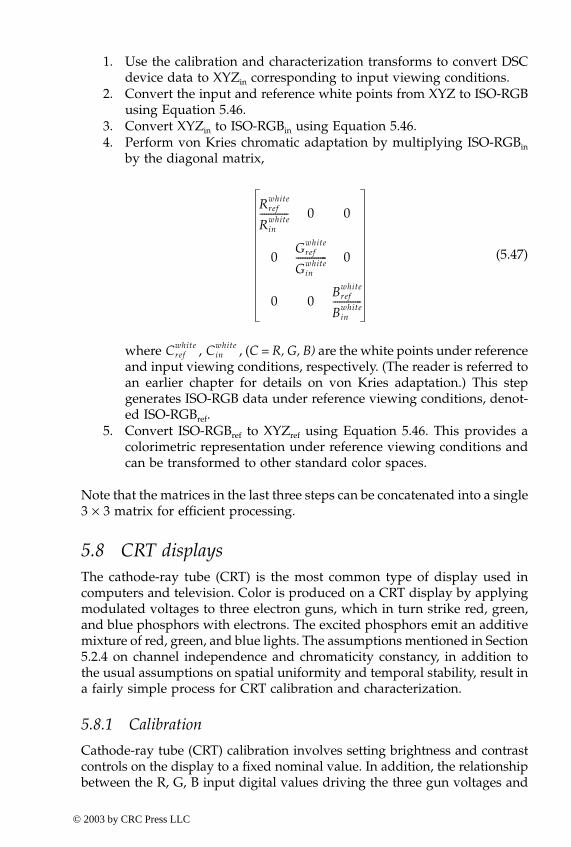
324 Digital Color Imaging Handbook
1. Use the calibration and characterization transforms to convert DSCdevice data to XYZin corresponding to input viewing conditions.
2. Convert the input and reference white points from XYZ to ISO-RGBusing Equation 5.46.
3. Convert XYZin to ISO-RGBin using Equation 5.46.4. Perform von Kries chromatic adaptation by multiplying ISO-RGBin
by the diagonal matrix,
(5.47)
where , , (C = R, G, B) are the white points under referenceand input viewing conditions, respectively. (The reader is referred toan earlier chapter for details on von Kries adaptation.) This stepgenerates ISO-RGB data under reference viewing conditions, denot-ed ISO-RGBref.
5. Convert ISO-RGBref to XYZref using Equation 5.46. This provides acolorimetric representation under reference viewing conditions andcan be transformed to other standard color spaces.
Note that the matrices in the last three steps can be concatenated into a single3 × 3 matrix for efficient processing.
5.8 CRT displaysThe cathode-ray tube (CRT) is the most common type of display used incomputers and television. Color is produced on a CRT display by applyingmodulated voltages to three electron guns, which in turn strike red, green,and blue phosphors with electrons. The excited phosphors emit an additivemixture of red, green, and blue lights. The assumptions mentioned in Section5.2.4 on channel independence and chromaticity constancy, in addition tothe usual assumptions on spatial uniformity and temporal stability, result ina fairly simple process for CRT calibration and characterization.
5.8.1 Calibration
Cathode-ray tube (CRT) calibration involves setting brightness and contrastcontrols on the display to a fixed nominal value. In addition, the relationshipbetween the R, G, B input digital values driving the three gun voltages and
Rrefwhite
Rinwhite
------------- 0 0
0Gref
white
Ginwhite
-------------- 0
0 0Bref
white
Binwhite
-------------
Crefwhite Cin
white
-ColorBook Page 324 Wednesday, November 13, 2002 10:55 AM
© 2003 by CRC Press LLC
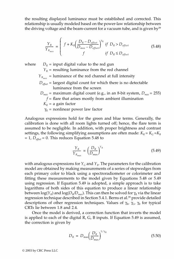
Chapter five: Device characterization 325
the resulting displayed luminance must be established and corrected. Thisrelationship is usually modeled based on the power-law relationship betweenthe driving voltage and the beam-current for a vacuum tube, and is given by39
(5.48)
where DR = input digital value to the red gun YR = resulting luminance from the red channel
= luminance of the red channel at full intensity
Doffset = largest digital count for which there is no detectable luminance from the screen
Dmax = maximum digital count (e.g., in an 8-bit system, Dmax = 255)f = flare that arises mostly from ambient illumination
KR = a gain factorγR = nonlinear power law factor
Analogous expressions hold for the green and blue terms. Generally, thecalibration is done with all room lights turned off; hence, the flare term isassumed to be negligible. In addition, with proper brightness and contrastsettings, the following simplifying assumptions are often made: KR = KG =KB
= 1, Doffset = 0. This reduces Equation 5.48 to
(5.49)
with analogous expressions for YG and YB. The parameters for the calibrationmodel are obtained by making measurements of a series of stepwedges fromeach primary color to black using a spectroradiometer or colorimeter andfitting these measurements to the model given by Equations 5.48 or 5.49using regression. If Equation 5.49 is adopted, a simple approach is to takelogarithms of both sides of this equation to produce a linear relationshipbetween log(YR) and log(DR/Dmax). This can then be solved for γR via the linearregression technique described in Section 5.4.1. Berns et al.39 provide detaileddescriptions of other regression techniques. Values of γR, γG, γB for typicalCRTs lie between 1.8 and 2.4.
Once the model is derived, a correction function that inverts the modelis applied to each of the digital R, G, B inputs. If Equation 5.49 is assumed,the correction is given by
(5.50)
YR
YRmax
------------ f KR+DR Doffset–
Dmax Doffset–--------------------------------
γR
if DR Doffset>
f if DR Doffset≤
=
YRmax
YR
YRmax
------------DR
Dmax------------
YR
=
DR DmaxDR
,
Dmax------------
1/γR
=
-ColorBook Page 325 Wednesday, November 13, 2002 10:55 AM
© 2003 by CRC Press LLC
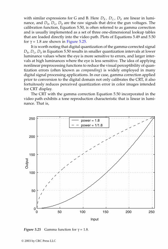
326 Digital Color Imaging Handbook
with similar expressions for G and B. Here , , are linear in lumi-nance, and DR, DG, DB are the raw signals that drive the gun voltages. Thecalibration function, Equation 5.50, is often referred to as gamma correctionand is usually implemented as a set of three one-dimensional lookup tablesthat are loaded directly into the video path. Plots of Equations 5.49 and 5.50for γ = 1.8 are shown in Figure 5.25.
It is worth noting that digital quantization of the gamma-corrected signalDR, DG, DB in Equation 5.50 results in smaller quantization intervals at lowerluminance values where the eye is more sensitive to errors, and larger inter-vals at high luminances where the eye is less sensitive. The idea of applyingnonlinear preprocessing functions to reduce the visual perceptibility of quan-tization errors (often known as companding) is widely employed in manydigital signal processing applications. In our case, gamma correction appliedprior to conversion to the digital domain not only calibrates the CRT, it alsofortuitously reduces perceived quantization error in color images intendedfor CRT display.
The CRT with the gamma correction Equation 5.50 incorporated in thevideo path exhibits a tone reproduction characteristic that is linear in lumi-nance. That is,
DR, DG
, DB,
0 50 100 150 200 2500
50
100
150
200
250
Input
Out
put
power = 1.8power = 1/1.8
Figure 5.25 Gamma function for γ = 1.8.
-ColorBook Page 326 Wednesday, November 13, 2002 10:55 AM
© 2003 by CRC Press LLC
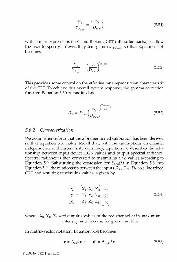
Chapter five: Device characterization 327
(5.51)
with similar expressions for G and B. Some CRT calibration packages allowthe user to specify an overall system gamma, γsystem, so that Equation 5.51becomes
(5.52)
This provides some control on the effective tone reproduction characteristicof the CRT. To achieve this overall system response, the gamma correctionfunction Equation 5.50 is modified as
(5.53)
5.8.2 Characterization
We assume henceforth that the aforementioned calibration has been derivedso that Equation 5.51 holds. Recall that, with the assumptions on channelindependence and chromaticity constancy, Equation 5.8 describes the rela-tionship between input device RGB values and output spectral radiance.Spectral radiance is then converted to tristimulus XYZ values according toEquation 5.9. Substituting the expression for SRGB(λ) in Equation 5.8 intoEquation 5.9., the relationship between the inputs , , to a linearizedCRT and resulting tristimulus values is given by
(5.54)
where XR, YR, ZR = tristimulus values of the red channel at its maximum intensity, and likewise for green and blue
In matrix-vector notation, Equation 5.54 becomes
c = ACRT d’; d’ = ACRT–1
c (5.55)
YR
YRMax
------------DR
,
Dmax------------
=
YR
YRmax
------------DR
,
Dmax-----------
γ system
=
DR DmaxDR
,
Dmax-----------
γ systemγR
------------------
=
DR, DG
, DB,
XYZ
XR XG XB
YR YG YB
ZR ZG ZB
=
DR,
DG,
DB,
-ColorBook Page 327 Wednesday, November 13, 2002 10:55 AM
© 2003 by CRC Press LLC
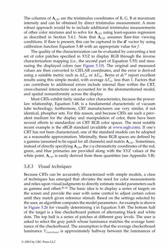
328 Digital Color Imaging Handbook
The columns of ACRT are the tristimulus coordinates of R, G, B at maximumintensity and can be obtained by direct tristimulus measurement. A morerobust approach would be to include additional tristimulus measurementsof other color mixtures and to solve for ACRT using least-squares regressionas described in Section 5.4.1. Note that ACRT assumes flare-free viewingconditions. If flare is present, this can be captured in the d’ vector by usingcalibration function Equation 5.48 with an appropriate value for f.
The quality of the characterization can be evaluated by converting a testset of color patches specified in XYZ to display RGB through the inversecharacterization mapping (i.e., the second part of Equation 5.55) and mea-suring the displayed colors (see Figure 5.10). The original and measuredvalues are then converted to CIELAB coordinates, and the error is derivedusing a suitable metric such as ∆ or ∆ . Berns et al.39 report excellentresults using this simple model, with average ∆ less than 1. Factors thatcan contribute to additional errors include internal flare within the CRT,cross-channel interactions not accounted for in the aforementioned model,and spatial nonuniformity across the display.
Most CRTs exhibit fairly similar color characteristics, because the power-law relationship, Equation 5.48, is a fundamental characteristic of vacuumtube technology; furthermore, CRT manufacturers use very similar, if notidentical, phosphor sets. For this reason, and because CRTs are such a prev-alent medium for the display and manipulation of color, there have beenseveral efforts to standardize on CRT RGB color spaces. The most notablerecent example is the sRGB standard (available at www.srgb.com). If one’sCRT has not been characterized, one of the standard models can be adoptedas a reasonable approximation. Minimally, these RGB spaces are defined bya gamma (assumed to be equal for all channels) and matrix ACRT . Sometimes,instead of directly specifying ACRT, the x-y chromaticity coordinates of the red,green, and blue primaries are provided along with the XYZ values of thewhite point. ACRT is easily derived from these quantities (see Appendix 5.B).
5.8.3 Visual techniques
Because CRTs can be accurately characterized with simple models, a classof techniques has emerged that obviates the need for color measurementsand relies upon visual judgments to directly estimate model parameters suchas gamma and offset.40–42 The basic idea is to display a series of targets onthe screen and provide the user with some control to adjust certain colorsuntil they match given reference stimuli. Based on the settings selected bythe user, an algorithm computes the model parameters. An example is shownin Figure 5.26 for visually determining γ in Equation 5.49. The bottom halfof the target is a fine checkerboard pattern of alternating black and whitedots. The top half is a series of patches at different gray levels. The user isasked to select the gray patch whose luminance matches the average lumi-nance of the checkerboard. The assumption is that the average checkerboardluminance Ycheckerboard is approximately halfway between the luminances of
Eab* E94
*
Eab*
-ColorBook Page 328 Wednesday, November 13, 2002 10:55 AM
© 2003 by CRC Press LLC
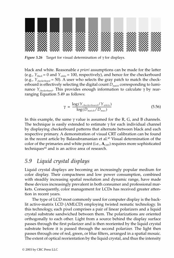
Chapter five: Device characterization 329
black and white. Reasonable a priori assumptions can be made for the latter(e.g., Yblack = 0 and Ywhite = 100, respectively), and hence for the checkerboard(e.g., Ycheckerboard = 50). A user who selects the gray patch to match the check-erboard is effectively selecting the digital count Dmatch corresponding to lumi-nance Ycheckerboard. This provides enough information to calculate γ by rear-ranging Equation 5.49 as follows:
(5.56)
In this example, the same γ value is assumed for the R, G, and B channels.The technique is easily extended to estimate γ for each individual channelby displaying checkerboard patterns that alternate between black and eachrespective primary. A demonstration of visual CRT calibration can be foundin the recent article by Balasubramanian et al.43 Visual determination of thecolor of the primaries and white point (i.e., ACRT) requires more sophisticatedtechniques44 and is an active area of research.
5.9 Liquid crystal displaysLiquid crystal displays are becoming an increasingly popular medium forcolor display. Their compactness and low power consumption, combinedwith steadily increasing spatial resolution and dynamic range, have madethese devices increasingly prevalent in both consumer and professional mar-kets. Consequently, color management for LCDs has received greater atten-tion in recent years.
The type of LCD most commonly used for computer display is the back-lit active-matrix LCD (AMLCD) employing twisted nematic technology. Inthis technology, each pixel comprises a pair of linear polarizers and a liquidcrystal substrate sandwiched between them. The polarizations are orientedorthogonally to each other. Light from a source behind the display surfacepasses through the first polarizer and is then reoriented by the liquid crystalsubstrate before it is passed through the second polarizer. The light thenpasses through one of red, green, or blue filters, arranged in a spatial mosaic.The extent of optical reorientation by the liquid crystal, and thus the intensity
Figure 5.26 Target for visual determination of γ for displays.
γYcheckerboard/Ywhite( )log
Dmatch/Dmax( )log----------------------------------------------------------=
-ColorBook Page 329 Wednesday, November 13, 2002 10:55 AM
© 2003 by CRC Press LLC
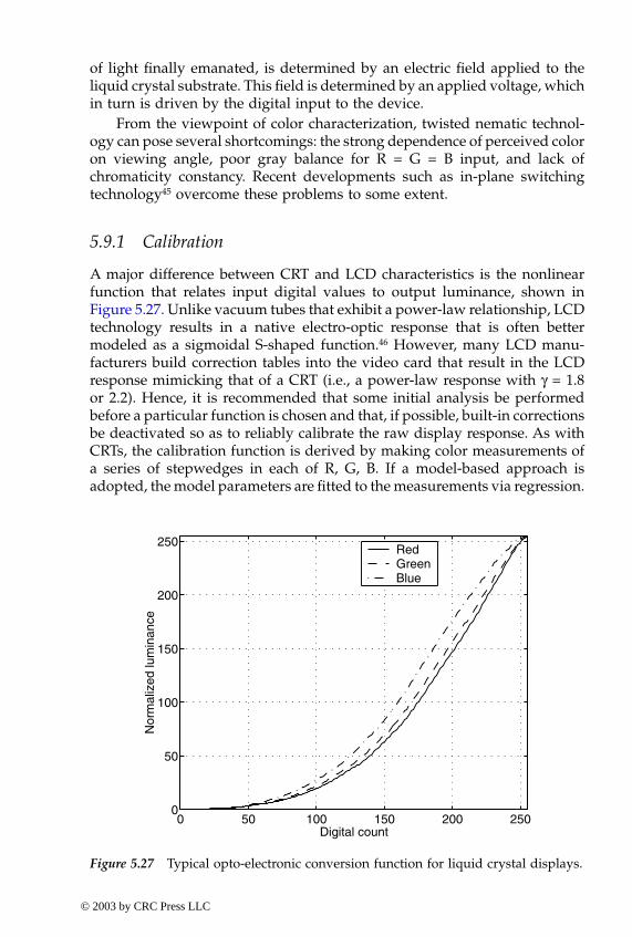
330 Digital Color Imaging Handbook
of light finally emanated, is determined by an electric field applied to theliquid crystal substrate. This field is determined by an applied voltage, whichin turn is driven by the digital input to the device.
From the viewpoint of color characterization, twisted nematic technol-ogy can pose several shortcomings: the strong dependence of perceived coloron viewing angle, poor gray balance for R = G = B input, and lack ofchromaticity constancy. Recent developments such as in-plane switchingtechnology45 overcome these problems to some extent.
5.9.1 Calibration
A major difference between CRT and LCD characteristics is the nonlinearfunction that relates input digital values to output luminance, shown inFigure 5.27. Unlike vacuum tubes that exhibit a power-law relationship, LCDtechnology results in a native electro-optic response that is often bettermodeled as a sigmoidal S-shaped function.46 However, many LCD manu-facturers build correction tables into the video card that result in the LCDresponse mimicking that of a CRT (i.e., a power-law response with γ = 1.8or 2.2). Hence, it is recommended that some initial analysis be performedbefore a particular function is chosen and that, if possible, built-in correctionsbe deactivated so as to reliably calibrate the raw display response. As withCRTs, the calibration function is derived by making color measurements ofa series of stepwedges in each of R, G, B. If a model-based approach isadopted, the model parameters are fitted to the measurements via regression.
0 50 100 150 200 2500
50
100
150
200
250
Digital count
Nor
mal
ized
lum
inan
ce
RedGreenBlue
Figure 5.27 Typical opto-electronic conversion function for liquid crystal displays.
-ColorBook Page 330 Wednesday, November 13, 2002 10:55 AM
© 2003 by CRC Press LLC
Chapter five: Device characterization 331
Alternatively, if the LCD response does not appear to subscribe to a simpleparametric model, an empirical approach may be adopted wherein the mea-sured data are directly interpolated or fitted using, for example, piecewiselinear, polynomial, or spline functions.
As mentioned earlier, some LCDs do not adhere to the chromaticityconstancy assumption. This is largely due to the non-smooth spectral char-acteristics of the backlight and its interaction with the color filters.45 Kwaket al.47 compensate for the lack of chromaticity constancy by introducingcross terms in the nonlinear calibration functions to capture interactionsamong R, G, and B. They claim a significant improvement in overall accuracyas a result of this extension.
5.9.2 Characterization
Most of the assumptions made with CRTs (i.e., uniformity, stability, pixelindependence, and channel independence) hold to a reasonable degree withAMLCDs as well. Hence, the characterization function can be modeled witha 3 × 3 matrix as in Equation 5.54, and the procedure described in Section5.8 for deriving CRT characterization can be used for AMLCDs in the samemanner. As mentioned earlier, an important caution for AMLCDs is that theradiance of the emanated light can be a strong function of the viewing angle.The only practical recommendation to mitigate this problem is that themeasurements should be taken of light emanating perpendicular to the planeof the screen. The same geometry should be used for viewing images. Forfurther details on LCD characterization, the reader is referred to the worksby Marcu,45 Sharma,46 and Kwak.47
5.10 Printers
Printer characterization continues to be a challenging problem due to thecomplex nonlinear color characteristics of these devices. Space consider-ations do not permit a description of the physics of the numerous digitalprinting technologies. Instead, we will offer general techniques that applyto broad categories of devices (e.g., halftone vs. continuous tone; CMY vs.CMYK, etc.).
Recall the basic calibration and characterization workflow in Figure 5.9.The techniques for target generation and calibration and characterizationvary widely, offering a range of trade-offs between cost and accuracy. Aselection of common techniques will be presented in this section.
5.10.1 Calibration
Two common approaches are channel-independent and gray-balancedcalibration.
-ColorBook Page 331 Wednesday, November 13, 2002 10:55 AM
© 2003 by CRC Press LLC
332 Digital Color Imaging Handbook
5.10.1.1 Channel-independent calibrationIn this type of calibration, each channel i (i = cyan, magenta, yellow, etc.) isindependently linearized to a defined metric Mi. An example of such a metricis the ∆ color difference between the ith channel and medium white,defined as
(5.57)
where d = input digital levelcmedium = CIELAB measurement of the medium
ci(d) = CIELAB measurement of the ith colorant generated at digital level d
Note that, by definition, . Linearizing with respect to this metricwill result in an approximately visually linear printer response along eachof its primary channels.
The calibration is accomplished with the following steps:
• Generate stepwedges of pure C, M, Y patches at a few selected digitallevels dj. The number and spacing of levels required depend on thecharacteristics of the printer. As a general guideline, between 15 and20 patches per channel is sufficient for most printers, and a finersampling is recommended in the region of small d values to accu-rately capture the printer response at the highlights. Also ensure thatthe solid patch (i.e., d = dmax) is included.
• Make CIELAB measurements of the stepwedges and of the baremedium. Media relative colorimetry is recommended for the CIELABcalculations.
• Evaluate Mi(dj) at the measured digital levels dj using Equation 5.57.• Scale the data by a multiplicative factor so that Mi(dmax) = dmax. This
is accomplished by multiplying the function Mi(d) by the constant[dmax/Mi(dmax)].
• Invert the scaled functions Mi(d) to obtain Mi–1 by interchanging the
dependent and independent variables. Use some form of fitting orinterpolation to evaluate Mi
–1 for the entire domain [0, dmax]. If theprinter response is smooth, linear interpolation suffices; otherwise,more sophisticated fitting techniques such as polynomials or splinesare called for (see Section 5.4.). The result is the calibration function,which can be implemented as a set of one-dimensional TRCs forefficient processing of images.
• Test the calibration by running a stepwedge of uniformly spaceddigital values of a single colorant through the TRC, printing andmeasuring the resulting patches, and computing Mi. A linear rela-tionship should be achieved between the digital input to the TRCand the resulting Mi. Repeat this step for each colorant.
Eab*
Mi d( ) cmedium ci– d( ) 2, i C,M,Y,0 d dmax≤ ≤= =
Mi 0( ) 0≡
-ColorBook Page 332 Wednesday, November 13, 2002 10:55 AM
© 2003 by CRC Press LLC
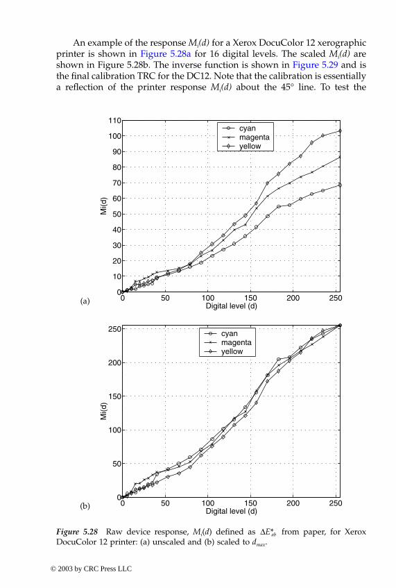
Chapter five: Device characterization 333
An example of the response Mi(d) for a Xerox DocuColor 12 xerographicprinter is shown in Figure 5.28a for 16 digital levels. The scaled Mi(d) areshown in Figure 5.28b. The inverse function is shown in Figure 5.29 and isthe final calibration TRC for the DC12. Note that the calibration is essentiallya reflection of the printer response Mi(d) about the 45° line. To test the
0 50 100 150 200 2500
10
20
30
40
50
60
70
80
90
100
110
Digital level (d)
Mi(d
)
cyanmagentayellow
0 50 100 150 200 2500
50
100
150
200
250
Digital level (d)
Mi(d
)
cyanmagentayellow
Figure 5.28 Raw device response, Mi(d) defined as ∆E*ab from paper, for XeroxDocuColor 12 printer: (a) unscaled and (b) scaled to dmax.
(a)
(b)
-ColorBook Page 333 Wednesday, November 13, 2002 10:55 AM
© 2003 by CRC Press LLC
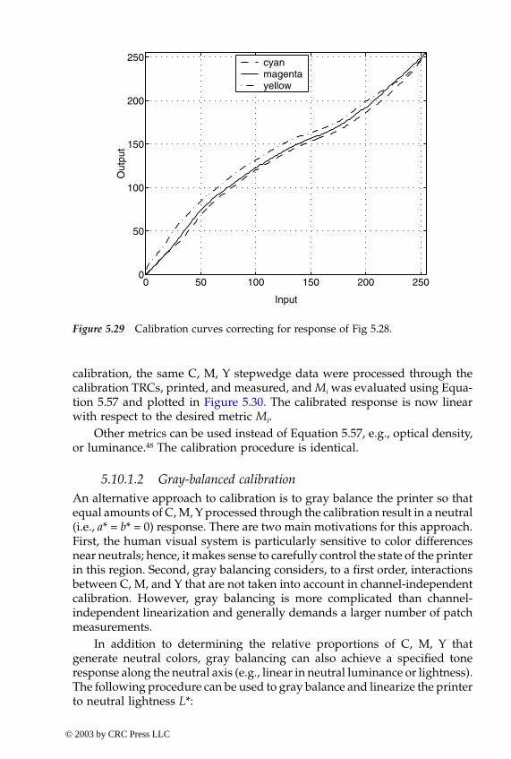
334 Digital Color Imaging Handbook
calibration, the same C, M, Y stepwedge data were processed through thecalibration TRCs, printed, and measured, and Mi was evaluated using Equa-tion 5.57 and plotted in Figure 5.30. The calibrated response is now linearwith respect to the desired metric Mi.
Other metrics can be used instead of Equation 5.57, e.g., optical density,or luminance.48 The calibration procedure is identical.
5.10.1.2 Gray-balanced calibrationAn alternative approach to calibration is to gray balance the printer so thatequal amounts of C, M, Y processed through the calibration result in a neutral(i.e., a* = b* = 0) response. There are two main motivations for this approach.First, the human visual system is particularly sensitive to color differencesnear neutrals; hence, it makes sense to carefully control the state of the printerin this region. Second, gray balancing considers, to a first order, interactionsbetween C, M, and Y that are not taken into account in channel-independentcalibration. However, gray balancing is more complicated than channel-independent linearization and generally demands a larger number of patchmeasurements.
In addition to determining the relative proportions of C, M, Y thatgenerate neutral colors, gray balancing can also achieve a specified toneresponse along the neutral axis (e.g., linear in neutral luminance or lightness).The following procedure can be used to gray balance and linearize the printerto neutral lightness L*:
0 50 100 150 200 2500
50
100
150
200
250
Input
Out
put
cyanmagentayellow
Figure 5.29 Calibration curves correcting for response of Fig 5.28.
-ColorBook Page 334 Wednesday, November 13, 2002 10:55 AM
© 2003 by CRC Press LLC
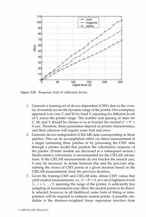
Chapter five: Device characterization 335
1. Generate a training set of device-dependent (CMY) data in the vicin-ity of neutrals across the dynamic range of the printer. One exemplaryapproach is to vary C and M for fixed Y, repeating for different levelsof Y across the printer range. The number and spacing of steps forC, M, and Y should be chosen so as to bracket the neutral a* = b* =0 axis. Therefore, these parameters depend on printer characteristics,and their selection will require some trial and error.
2. Generate device-independent (CIELAB) data corresponding to thesepatches. This can be accomplished either via direct measurement ofa target containing these patches or by processing the CMY datathrough a printer model that predicts the colorimetric response ofthe printer. (Printer models are discussed in a subsequent section.)Media-relative colorimetry is recommended for the CIELAB calcula-tions. If the CIELAB measurements do not bracket the neutral axis,it may be necessary to iterate between this and the previous step,refining the choice of CMY points at a given iteration based on theCIELAB measurements from the previous iteration.
3. Given the training CMY and CIELAB data, obtain CMY values thatyield neutral measurements, i.e., a* = b* = 0, at a set of lightness levels
, i = 1, …, T, spanning the range of the printer. A sufficiently finesampling of measurements may allow the neutral points to be direct-ly selected; however, in all likelihood, some form of fitting or inter-polation will be required to estimate neutral points. A possible can-didate is the distance-weighted linear regression function from
0 50 100 150 200 2500
10
20
30
40
50
60
70
80
90
100
110
Digital level (d)
Mi(d
)
cyanmagentayellow
Figure 5.30 Response Mi(d) of calibrated device.
Li*
-ColorBook Page 335 Wednesday, November 13, 2002 10:55 AM
© 2003 by CRC Press LLC
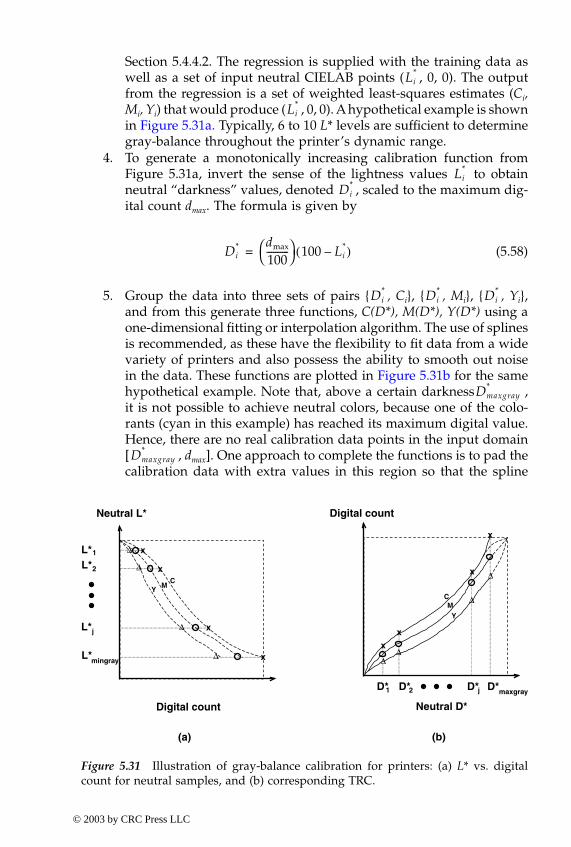
336 Digital Color Imaging Handbook
Section 5.4.4.2. The regression is supplied with the training data aswell as a set of input neutral CIELAB points ( , 0, 0). The outputfrom the regression is a set of weighted least-squares estimates (Ci,Mi, Yi) that would produce ( , 0, 0). A hypothetical example is shownin Figure 5.31a. Typically, 6 to 10 L* levels are sufficient to determinegray-balance throughout the printer’s dynamic range.
4. To generate a monotonically increasing calibration function fromFigure 5.31a, invert the sense of the lightness values to obtainneutral “darkness” values, denoted , scaled to the maximum dig-ital count dmax. The formula is given by
(5.58)
5. Group the data into three sets of pairs { , Ci}, { , Mi}, { , Yi},and from this generate three functions, C(D*), M(D*), Y(D*) using aone-dimensional fitting or interpolation algorithm. The use of splinesis recommended, as these have the flexibility to fit data from a widevariety of printers and also possess the ability to smooth out noisein the data. These functions are plotted in Figure 5.31b for the samehypothetical example. Note that, above a certain darkness ,it is not possible to achieve neutral colors, because one of the colo-rants (cyan in this example) has reached its maximum digital value.Hence, there are no real calibration data points in the input domain[ , dmax]. One approach to complete the functions is to pad thecalibration data with extra values in this region so that the spline
Li*
Li*
x
∆
x
x
x
∆
∆
∆
Neutral L*
Digital count
L*mingray
L*1
L*2
L*j
Digital count
Neutral D*
D*1 D*2 D*maxgray
xx
x
∆
∆
x
∆∆
(a) (b)
D*j
CM
YCM
Y
Figure 5.31 Illustration of gray-balance calibration for printers: (a) L* vs. digitalcount for neutral samples, and (b) corresponding TRC.
Li*
Di*
Di* dmax
100----------
100 Li*–( )=
Di* Di
* Di*
Dmaxgray*
Dmaxgray*
-ColorBook Page 336 Wednesday, November 13, 2002 10:55 AM
© 2003 by CRC Press LLC
Chapter five: Device characterization 337
fitting will smoothly extrapolate to the endpoint, dmax. Figure 5.31bshows schematically the extrapolation with dashed lines. To achievesmooth calibration functions, it may be necessary to sacrifice graybalance for some darkness values less than . In the case ofCMYK printers, the trade-off can be somewhat mitigated by usingthe K channel in combination with C, M, Y to achieve gray balance.Trade-offs between smoothness and colorimetric accuracy are fre-quently encountered in printer calibration and characterization. Un-fortunately, there is no universal solution to such issues; instead,knowledge of the particular printer and user requirements is used toheuristically guide the trade-offs.
6. Test the calibration by processing a stepwedge of samples C = M =Y = d through the TRCs, and printing and measuring CIELAB values.As before, it is convenient to assess the outcome by plotting L*, a*,b* as a function of the input digital count d. For most of the range
, the calibration should yield a linear response with respectto L*, and . If the deviation from this ideal aim is withinthe inherent variability of the system (e.g., the stability and unifor-mity of the printer), the calibration is of satisfactory accuracy. Recallthat, for gray levels darker than , a linear gray-balanced re-sponse is no longer achievable; instead, the printer response shouldsmoothly approach the color of the CMY solid overprint.
7. An additional test, highly recommended for gray-balance calibration,is to generate a target of continuous ramps of C = M = Y, processthrough the calibration, print, and visually inspect the output to en-sure a smooth neutral response. The prints must be viewed under thesame illuminant used for the CIELAB calculations in the calibration.
A recent study by the author has shown that visual tolerance for gray inreflection prints is not symmetric about the a* = b* = 0 point.49 In fact, people’smemory of and preference for gray occurs in the quadrant corresponding toa* < 0, b* < 0. In regions corresponding to positive a* or b*, a dominant hueis more readily perceived; hence, tolerances for gray reproduction in theseregions are small. Colloquially phrased, people prefer “cooler” (blu-ish/greenish) grays to “warmer” (reddish/yellowish) grays. This observa-tion can exploited to improve the robustness of gray balancing for printers.The device could be balanced toward preferred gray (a*, b* < 0) rather thancolorimetric gray (a* = b* = 0) with the same procedure described above.The expected advantage is that, by setting the calibration aim-point in aregion with large visual tolerance, the errors inevitably introduced by thecalibration are less likely to be visually objectionable.
5.10.2 Model-based printer characterization
Several physics-based models have been developed to predict the colorimet-ric response of a printer. Some of the common models will be described in
Dmaxgray*
0 d D*≤ ≤a*, b* 0≈
Dmax*
-ColorBook Page 337 Wednesday, November 13, 2002 10:55 AM
© 2003 by CRC Press LLC
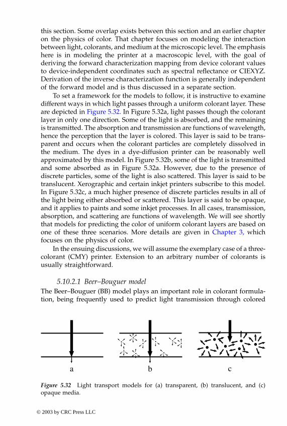
338 Digital Color Imaging Handbook
this section. Some overlap exists between this section and an earlier chapteron the physics of color. That chapter focuses on modeling the interactionbetween light, colorants, and medium at the microscopic level. The emphasishere is in modeling the printer at a macroscopic level, with the goal ofderiving the forward characterization mapping from device colorant valuesto device-independent coordinates such as spectral reflectance or CIEXYZ.Derivation of the inverse characterization function is generally independentof the forward model and is thus discussed in a separate section.
To set a framework for the models to follow, it is instructive to examinedifferent ways in which light passes through a uniform colorant layer. Theseare depicted in Figure 5.32. In Figure 5.32a, light passes though the colorantlayer in only one direction. Some of the light is absorbed, and the remainingis transmitted. The absorption and transmission are functions of wavelength,hence the perception that the layer is colored. This layer is said to be trans-parent and occurs when the colorant particles are completely dissolved inthe medium. The dyes in a dye-diffusion printer can be reasonably wellapproximated by this model. In Figure 5.32b, some of the light is transmittedand some absorbed as in Figure 5.32a. However, due to the presence ofdiscrete particles, some of the light is also scattered. This layer is said to betranslucent. Xerographic and certain inkjet printers subscribe to this model.In Figure 5.32c, a much higher presence of discrete particles results in all ofthe light being either absorbed or scattered. This layer is said to be opaque,and it applies to paints and some inkjet processes. In all cases, transmission,absorption, and scattering are functions of wavelength. We will see shortlythat models for predicting the color of uniform colorant layers are based onone of these three scenarios. More details are given in Chapter 3, whichfocuses on the physics of color.
In the ensuing discussions, we will assume the exemplary case of a three-colorant (CMY) printer. Extension to an arbitrary number of colorants isusually straightforward.
5.10.2.1 Beer–Bouguer modelThe Beer–Bouguer (BB) model plays an important role in colorant formula-tion, being frequently used to predict light transmission through colored
a b c
. . .. ..... . .... .
Figure 5.32 Light transport models for (a) transparent, (b) translucent, and (c)opaque media.
-ColorBook Page 338 Wednesday, November 13, 2002 10:55 AM
© 2003 by CRC Press LLC
Chapter five: Device characterization 339
materials in liquid solutions. In digital color imaging, it is most applicablefor continuous-tone printing with transparent colorants and media (i.e., Fig-ure 5.32a). The underlying assumption is that the spatial rate of change oflight radiance as it passes through an absorbing colorant layer is proportionalto the radiance itself. Mathematically, this is given by
(5.59)
where Ix(λ) = radiance at position x within the colorant layerA(λ) = a proportionality factor given by
A(λ) = ξ w k(λ) (5.60)
where ξ = concentration of the colorantw = thickness of the colorant layer
k(λ) = spectral absorption coefficient of the colorant
Substituting Equation 5.60 into Equation 5.59 and integrating with respectto x over the thickness of the colorant, we obtain the following expressionfor the radiance I(λ) emerging from the colorant:
(5.61)
where I0(λ) is the radiance of light that would be transmitted in the absenceof the colorant, which can be expressed as the product of the incident lightIi(λ) and the bare transparency Tt(λ). Equation 5.61 essentially states that theamount of light absorption depends directly on the amount of absorbingmaterial within the colorant, which in turn is proportional to both the con-centration and thickness of the colorant layer. Often, the colorant thicknessw is assumed to be spatially constant and is folded into the absorptioncoefficient k(λ). To this end, we no longer explicitly include w in the analysis.
It is useful to introduce spectral transmittance T(λ) and optical densityD(λ) of a colorant layer.
(5.62)
For color mixtures, the additivity rule can be invoked, which states thatthe density of a colorant mixture is equal to the sum of the densities of theindividual colorants.50 For a CMY printer, we thus have
DCMY(λ) = Dt(λ) + 0.4343(ξC kC(λ) + ξM kM(λ) + ξY kY(λ)) (5.63)
dIx λ( )dx
---------------- A λ( )– Ix λ( )=
I λ( ) I0 λ( ) ξwk λ( )–( )exp Ii λ( )Tt λ( ) ξwk λ( )–( )exp= =
T λ( ) I λ( )Ii λ( )----------- Tt λ( ) ξk λ( )–( )exp ;= =
D λ( ) log10 T λ( )( )=Dt λ( ) 0.4343 ξ k λ( )+–=
-ColorBook Page 339 Wednesday, November 13, 2002 10:55 AM
© 2003 by CRC Press LLC
340 Digital Color Imaging Handbook
which can be written in terms of transmittance,
TCMY(λ) = Tt(λ) exp[–(ξC kC(λ) + ξM kM(λ) + ξY kY(λ))] (5.64)
The model can be extended to reflective prints under the assumption thatthere is no scattering of light within the paper. This yields
(5.65)
where RCMY(λ) and Rp(λ) are the spectral reflectances of the colorant mixtureand paper, respectively. Note that, in reality, most reflective media do exhibitscattering, hence reducing the accuracy of Equation 5.65.
For a given printer, the parameters of Equations 5.64 and 5.65 are esti-mated from measurements of selected patches. The procedure for a CMYreflection printer is as follows:
• Measure the spectral reflectance of the paper, Rp(λ), and solid C, M,Y patches, RC(λ), RM(λ), RY(λ).
• Estimate the spectral absorption coefficient kC(λ) for the cyan colo-rant. This is done by setting ξC = 1, ξM = ξY = 0 in Equation 5.65 to yield
(5.66)
Use analogous expressions to derive kM(λ) and kY(λ).
• Derive the relationship between input digital level dj and cyan con-centration ξCj by printing a stepwedge of pure cyan patches at dif-ferent digital levels dj, and measure spectral reflectances RCj(λ). FromEquation 5.65, we know that
(5.67)
The quantity on the left is the absorption corresponding to concen-tration at level dj; hence, we denote this as kCj(λ). A least-squaresestimate for ξCj can be computed by minimizing the error.
(5.68)
where the summation is overall measured wavelengths within thevisible spectrum. Using the least-squares analysis in Appendix 5.A,the optimal ξCj is given by
RCMY λ( ) Rp λ( ) ξ( CkC λ( ) ξMkM λ( ) ξYkY λ( ) )+ +–[ ]exp=
kC λ( )RC λ( )Rp λ( )---------------
log–=
RCj λ( )Rp λ( )----------------
log– ξCjkC λ( )=
kCj λ( ) ξCjkC λ( )– 2
λ∑
-ColorBook Page 340 Wednesday, November 13, 2002 10:55 AM
© 2003 by CRC Press LLC
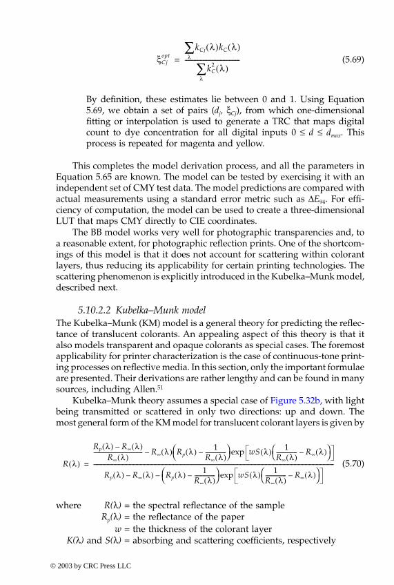
Chapter five: Device characterization 341
(5.69)
By definition, these estimates lie between 0 and 1. Using Equation5.69, we obtain a set of pairs (dj, ξCj), from which one-dimensionalfitting or interpolation is used to generate a TRC that maps digitalcount to dye concentration for all digital inputs 0 ≤ d ≤ dmax. Thisprocess is repeated for magenta and yellow.
This completes the model derivation process, and all the parameters inEquation 5.65 are known. The model can be tested by exercising it with anindependent set of CMY test data. The model predictions are compared withactual measurements using a standard error metric such as ∆E94. For effi-ciency of computation, the model can be used to create a three-dimensionalLUT that maps CMY directly to CIE coordinates.
The BB model works very well for photographic transparencies and, toa reasonable extent, for photographic reflection prints. One of the shortcom-ings of this model is that it does not account for scattering within colorantlayers, thus reducing its applicability for certain printing technologies. Thescattering phenomenon is explicitly introduced in the Kubelka–Munk model,described next.
5.10.2.2 Kubelka–Munk modelThe Kubelka–Munk (KM) model is a general theory for predicting the reflec-tance of translucent colorants. An appealing aspect of this theory is that italso models transparent and opaque colorants as special cases. The foremostapplicability for printer characterization is the case of continuous-tone print-ing processes on reflective media. In this section, only the important formulaeare presented. Their derivations are rather lengthy and can be found in manysources, including Allen.51
Kubelka–Munk theory assumes a special case of Figure 5.32b, with lightbeing transmitted or scattered in only two directions: up and down. Themost general form of the KM model for translucent colorant layers is given by
(5.70)
where R(λ) = the spectral reflectance of the sampleRp(λ) = the reflectance of the paper
w = the thickness of the colorant layerK(λ) and S(λ) = absorbing and scattering coefficients, respectively
ξCjopt
kCj λ( )λ∑ kC λ( )
kC2 λ( )
λ∑
------------------------------------=
R λ( )
Rp λ( ) R∞ λ( )–R∞ λ( )
------------------------------------ R∞ λ( )– Rp λ( ) 1R∞ λ( )---------------–
wS λ( ) 1R∞ λ( )--------------- R∞ λ( )–
exp
Rp λ( ) R∞ λ( )– Rp λ( ) 1R∞ λ( )---------------–
wS λ( ) 1R∞ λ( )--------------- R∞ λ( )–
exp–-------------------------------------------------------------------------------------------------------------------------------------------------------------------------------=
-ColorBook Page 341 Wednesday, November 13, 2002 10:55 AM
© 2003 by CRC Press LLC
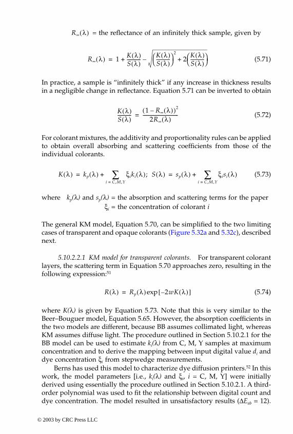
342 Digital Color Imaging Handbook
= the reflectance of an infinitely thick sample, given by
(5.71)
In practice, a sample is “infinitely thick” if any increase in thickness resultsin a negligible change in reflectance. Equation 5.71 can be inverted to obtain
(5.72)
For colorant mixtures, the additivity and proportionality rules can be appliedto obtain overall absorbing and scattering coefficients from those of theindividual colorants.
(5.73)
where kp(λ) and sp(λ) = the absorption and scattering terms for the paperξi = the concentration of colorant i
The general KM model, Equation 5.70, can be simplified to the two limitingcases of transparent and opaque colorants (Figure 5.32a and 5.32c), describednext.
5.10.2.2.1 KM model for transparent colorants. For transparent colorantlayers, the scattering term in Equation 5.70 approaches zero, resulting in thefollowing expression:51
(5.74)
where K(λ) is given by Equation 5.73. Note that this is very similar to theBeer–Bouguer model, Equation 5.65. However, the absorption coefficients inthe two models are different, because BB assumes collimated light, whereasKM assumes diffuse light. The procedure outlined in Section 5.10.2.1 for theBB model can be used to estimate ki(λ) from C, M, Y samples at maximumconcentration and to derive the mapping between input digital value di anddye concentration ξi from stepwedge measurements.
Berns has used this model to characterize dye diffusion printers.52 In thiswork, the model parameters [i.e., ki(λ) and ξi, i = C, M, Y] were initiallyderived using essentially the procedure outlined in Section 5.10.2.1. A third-order polynomial was used to fit the relationship between digital count anddye concentration. The model resulted in unsatisfactory results (∆Eab = 12).
R∞ λ( )
R∞ λ( ) 1 K λ( )S λ( )------------
K λ( )S λ( )------------
2
2 K λ( )S λ( )------------
+–+=
K λ( )S λ( )------------
1 R∞ λ( )–( )2
2R∞ λ( )-------------------------------=
K λ( ) kp λ( ) ξiki λ( )i C ,M ,Y=
∑ ; S λ( )+ sp λ( ) ξisi λ( )i C ,M ,Y=
∑+= =
R λ( ) Rp λ( ) 2wK λ( )–[ ]exp=
-ColorBook Page 342 Wednesday, November 13, 2002 10:55 AM
© 2003 by CRC Press LLC
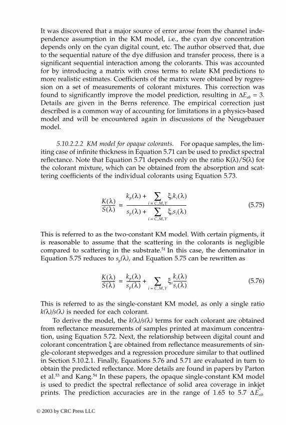
Chapter five: Device characterization 343
It was discovered that a major source of error arose from the channel inde-pendence assumption in the KM model, i.e., the cyan dye concentrationdepends only on the cyan digital count, etc. The author observed that, dueto the sequential nature of the dye diffusion and transfer process, there is asignificant sequential interaction among the colorants. This was accountedfor by introducing a matrix with cross terms to relate KM predictions tomore realistic estimates. Coefficients of the matrix were obtained by regres-sion on a set of measurements of colorant mixtures. This correction wasfound to significantly improve the model prediction, resulting in ∆Eab = 3.Details are given in the Berns reference. The empirical correction justdescribed is a common way of accounting for limitations in a physics-basedmodel and will be encountered again in discussions of the Neugebauermodel.
5.10.2.2.2 KM model for opaque colorants. For opaque samples, the lim-iting case of infinite thickness in Equation 5.71 can be used to predict spectralreflectance. Note that Equation 5.71 depends only on the ratio K(λ)/S(λ) forthe colorant mixture, which can be obtained from the absorption and scat-tering coefficients of the individual colorants using Equation 5.73.
(5.75)
This is referred to as the two-constant KM model. With certain pigments, itis reasonable to assume that the scattering in the colorants is negligiblecompared to scattering in the substrate.51 In this case, the denominator inEquation 5.75 reduces to sp(λ), and Equation 5.75 can be rewritten as
(5.76)
This is referred to as the single-constant KM model, as only a single ratiok(λ)/s(λ) is needed for each colorant.
To derive the model, the k(λ)/s(λ) terms for each colorant are obtainedfrom reflectance measurements of samples printed at maximum concentra-tion, using Equation 5.72. Next, the relationship between digital count andcolorant concentration ξ are obtained from reflectance measurements of sin-gle-colorant stepwedges and a regression procedure similar to that outlinedin Section 5.10.2.1. Finally, Equations 5.76 and 5.71 are evaluated in turn toobtain the predicted reflectance. More details are found in papers by Partonet al.53 and Kang.54 In these papers, the opaque single-constant KM modelis used to predict the spectral reflectance of solid area coverage in inkjetprints. The prediction accuracies are in the range of 1.65 to 5.7 ∆
K λ( )S λ( )------------
kp λ( ) ξiki λ( )i C ,M ,Y=
∑+
sp λ( ) ξisi λ( )i C ,M ,Y=
∑+------------------------------------------------------=
K λ( )S λ( )------------
kp λ( )sp λ( )------------- ξi
ki λ( )si λ( )------------
i C ,M ,Y=∑+=
Eab*
-ColorBook Page 343 Wednesday, November 13, 2002 10:55 AM
© 2003 by CRC Press LLC
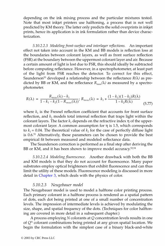
344 Digital Color Imaging Handbook
depending on the ink mixing process and the particular mixtures tested.Note that most inkjet printers use halftoning, a process that is not wellpredicted by KM theory. The latter only predicts the solid overprints in inkjetprints, hence its application is in ink formulation rather than device charac-terization.
5.10.2.2.3 Modeling front-surface and interlayer reflections. An importanteffect not taken into account in the KM and BB models is reflection loss atthe boundaries between colorant layers, as well as front surface reflection(FSR) at the boundary between the uppermost colorant layer and air. Becausea certain amount of light is lost due to FSR, this should ideally be subtractedbefore computing reflectance. However, in a spectrophotometer, at least partof the light from FSR reaches the detector. To correct for this effect,Saunderson55 developed a relationship between the reflectance R(λ) as pre-dicted by BB or KM, and the reflectance Rmeas(λ) as measured by a spectro-photometer.
(5.77)
where k1 is the Fresnel reflection coefficient that accounts for front surfacereflection, and k2 models total internal reflection that traps light within thecolorant layers. The factor k1 depends on the refractive index η of the upper-most colorant layer. A common assumption for η is 1.5, which correspondsto k1 = 0.04. The theoretical value of k2 for the case of perfectly diffuse lightis 0.6.51 Alternatively, these parameters can be chosen to provide the bestempirical fit between measured and modeled reflectance data.
The Saunderson correction is performed as a final step after deriving theBB or KM, and it has been shown to improve model accuracy.52,54
5.10.2.2.4 Modeling fluorescence. Another drawback with both the BBand KM models is that they do not account for fluorescence. Many papersubstrates employ optical brighteners that exhibit fluorescence and can thuslimit the utility of these models. Fluorescence modeling is discussed in moredetail in Chapter 3, which deals with the physics of color.
5.10.2.3 Neugebauer modelThe Neugebauer model is used to model a halftone color printing process.Each primary colorant in a halftone process is rendered as a spatial patternof dots, each dot being printed at one of a small number of concentrationlevels. The impression of intermediate levels is achieved by modulating thesize, shape, and spatial frequency of the dots. (Techniques for color halfton-ing are covered in more detail in a subsequent chapter.)
A process employing N colorants at Q concentration levels results in oneof QN colorant combinations being printed at any given spatial location. Webegin the formulation with the simplest case of a binary black-and-white
R λ( )Rmeas λ( ) k1–
1 k1 k2 1 Rmeas λ( )–( )––----------------------------------------------------------- ;= Rmeas λ( ) k1
1 k1–( ) 1 k2–( )R λ( )1 k2R λ( )–
--------------------------------------------------+=
-ColorBook Page 344 Wednesday, November 13, 2002 10:55 AM
© 2003 by CRC Press LLC
Chapter five: Device characterization 345
printer. This corresponds to N = 1 and Q = 2 (zero or maximum) concentra-tion levels; thus, at any given spatial location, we have two possible colorantcombinations, black or white. The reflectance of a halftone pattern is pre-dicted by the Murray–Davies equation,50
R = (1 – k)Pp + kPk (5.78)
where k = fractional area covered by the black dotsPp, Pk = reflectances of paper and black colorant, respectively
The Neugebauer model is a straightforward extension of the Murray–Daviesequation to color halftone mixtures.56 Binary printers employing C, M, Ycolorants render one of 23 = 8 colorant combinations at a given spatiallocation. The set of colorant combinations is S = {P, C, M, Y, CM, MY, CY,CMY}, where P denotes paper white, C denotes solid cyan, CM denotes thecyan–magenta overprint, etc. The Neugebauer model predicts the reflectanceof a color halftone as a weighted average of the reflectances of the eightcolorant combinations.
(5.79)
where S = the aforementioned set of colorant combinationsPi = spectral reflectance of the ith colorant combination,
henceforth referred to as the ith Neugebauer primaryweight wi = the relative area coverage of the ith colorant combination,
which is dictated by the halftoning method used
In the original Neugebauer equations, the predicted color is specified bythree broadband reflectances representing the short, medium, and longwavelength portions of the electromagnetic spectrum. In this work, spec-trally narrowband reflectances are used instead of their broadband counter-parts, as the former generally yield greater accuracy.57 The spectral Neuge-bauer equations are
(5.80)
Because Pi(λ) are colors of solid overprints, they can be predicted from single-colorant measurements using the BB or KM theories described in the previ-ous sections. However, for any given set of colorants, there are only a smallnumber of such overprints; hence, they are usually measured directly.
5.10.2.3.1 Effect of halftone dot placement. A common assumption isthat the dot placements of the colorants are statistically independent; i.e.,
R wiPii S=∑=
R λ( ) wiPi λ( )i S∈∑=
-ColorBook Page 345 Wednesday, November 13, 2002 10:55 AM
© 2003 by CRC Press LLC
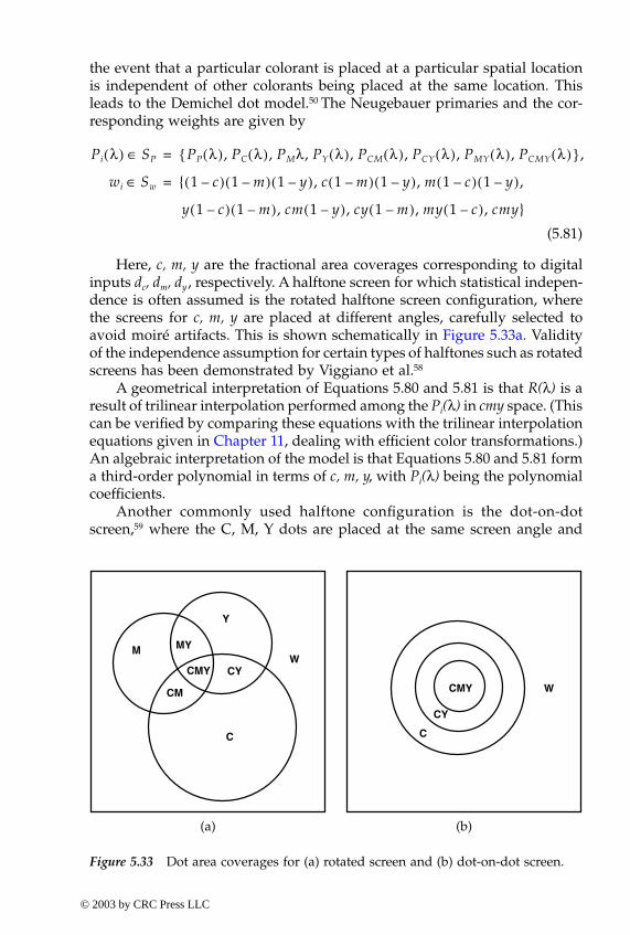
346 Digital Color Imaging Handbook
the event that a particular colorant is placed at a particular spatial locationis independent of other colorants being placed at the same location. Thisleads to the Demichel dot model.50 The Neugebauer primaries and the cor-responding weights are given by
(5.81)
Here, c, m, y are the fractional area coverages corresponding to digitalinputs dc, dm, dy , respectively. A halftone screen for which statistical indepen-dence is often assumed is the rotated halftone screen configuration, wherethe screens for c, m, y are placed at different angles, carefully selected toavoid moiré artifacts. This is shown schematically in Figure 5.33a. Validityof the independence assumption for certain types of halftones such as rotatedscreens has been demonstrated by Viggiano et al.58
A geometrical interpretation of Equations 5.80 and 5.81 is that R(λ) is aresult of trilinear interpolation performed among the Pi(λ) in cmy space. (Thiscan be verified by comparing these equations with the trilinear interpolationequations given in Chapter 11, dealing with efficient color transformations.)An algebraic interpretation of the model is that Equations 5.80 and 5.81 forma third-order polynomial in terms of c, m, y, with Pi(λ) being the polynomialcoefficients.
Another commonly used halftone configuration is the dot-on-dotscreen,59 where the C, M, Y dots are placed at the same screen angle and
Pi λ( ) SP∈ PP λ( ), PC λ( ), PMλ, PY λ( ), PCM λ( ), PCY λ( ), PMY λ( ), PCMY λ( ){ },=
wi Sw∈ { 1 c–( ) 1 m–( ) 1 y–( ), c 1 m–( ) 1 y–( ), m 1 c–( ) 1 y–( ),=
y 1 c–( ) 1 m–( ), cm 1 y–( ), cy 1 m–( ), my 1 c–( ), cmy}
MY
CMYW
M
CM
CY
Y
C
CMY W
CY
C
Figure 5.33 Dot area coverages for (a) rotated screen and (b) dot-on-dot screen.
(a) (b)
-ColorBook Page 346 Wednesday, November 13, 2002 10:55 AM
© 2003 by CRC Press LLC
Chapter five: Device characterization 347
phase as shown in Figure 5.33b. While the basic form of the mixing equationsis similar to Equation 5.80, the weights
w
i
are different from those of ran-domly positioned dots. Let X
i be the colorant with the
i th smallest areacoverage
a
i
. For example, if [c, m, y] = [0.8, 0.5, 0.2], then X
1 = Y, X
2
= M, X
3
= C; a
1
= 0.2, a
2
= 0.5, a
3 = 0.8. The set of Neugebauer primaries and corre-sponding weights are now given by
(5.82)
The final output reflectance in Equation 5.80 is now a summation of, at most,four terms.
Geometrically, Equation 5.82 represents tetrahedral interpolation amongthe
P
i
(
l
)
at four of the eight vertices of the
cmy cube. (This can be verifiedby comparing Equation 5.82 with the equations for tetrahedral interpolationgiven in the Chapter 11.) Different Neugebauer primaries are selected forthe calculation depending on the relative sizes of the area coverages
c, m, y
(equivalently, the tetrahedron to which the input
cmy
coordinate belongs).However, the weights
w
i
, and hence the resulting interpolated output
R(
l
),
are continuous as the input
cmy
coordinate moves from one tetrahedron toanother in
cmy
space. Algebraically, it is easily seen from Equations 5.80 and5.82 that, for fixed
l
,
R(
l
)
is a linear function of
c, m, y
, with the
P
i
(
l
)
beingthe weighting coefficients.
The aforementioned dot-on-dot mixing model assumes an ideal dotpattern with no noise, a perfectly rectangular dot density profile, and nomisregistration effects. In practice, these assumptions may be violated. It hasbeen shown
59
that a weighted mixture of the dot-on-dot and Demichel mix-ing models can effectively capture some of these effects. The new predictedreflectance is given by
R’(
l
) =
(1 –
a
)
R
dod
(
l
) +
a
R
dem
(
l
)
(5.83)
where
R
dod
(
l
)
= reflectance predicted by the dot-on-dot model
R
dem
(
l
)
= reflectance predicted by the Demichel model
a
= a weighting parameter that determines the relative proportions of the two mixing models; this factor can be chosen to fit the model to a set of measured data
As alluded to earlier, all these versions of the Neugebauer model easilygeneralize for an arbitrary number of colorants. For
N
colorants, theDemichel model for independent dot placement will result in the summationin Equation 5.80 containing 2
N
terms, while the dot-on-dot model contains
N
+ 1 terms.
Pi l( ) SP� PX1X2X3l( ), PX2X3
l( ), PX3l( ), Pw l( ){ }= ,
wi Sw� a1,a2 a1� ,a3 a2� ,1 a3�{ }=
05 Page 347 Monday, November 18, 2002 8:23 AM
© 2003 by CRC Press LLC
348 Digital Color Imaging Handbook
5.10.2.3.2 Effect of halftone screen frequency. The ideal Neugebauermodel assumes a perfect rectangular dot profile as a function of spatiallocation. In reality, dots have soft transitions from regions with full colorantto regions with no colorant. If the halftone screen frequency is relatively low,or a clustered dot is used, the relative area of the paper covered by thetransition regions is small, and the Neugebauer model would be expectedto be relatively accurate. On the other hand, if the screen frequency is high,or a dispersed dot is used, a relatively large fraction of the paper is coveredby transition regions, and the model breaks down. While some of the cor-rections discussed in following sections partially account for soft transitions,the reliability of the model has been seen to be greatest with clustered dotscreens with frequency less than 100 halftone dots per inch.
5.10.2.3.3 Effect of light scattering in the paper. An important pheno-menon not modeled by the basic Neugebauer equations is the scattering oflight within the paper. To understand this phenomenon, consider the inter-action of light with a black halftone print. The light that reaches the paperis given by
Ip = Iin(1 – k + kTk) (5.84)
where Iin = incident light intensityIp = light reaching the paperk = fractional black area coverage
Tk = transmittance of the black colorant
Figure 5. 34a shows the case where there is no optical scattering within thepaper. In this case, light incident on the print at a location containing colorantwill also exit through the colorant; likewise, light reaching the substrate willexit from the same location. The reflected light is thus given by
Irefl = Iin{(1 – k) Pp + k Tk2 Pp} (5.85)
where Pp is reflectance of the paper.Define the reflectance of the solid black colorant as Pk = Tk
2Pp. The overallreflectance is then given by the original Murray–Davies Equation 5.78.
Consider now the case where there is scattering within the paper, asshown in Figure 5.34b. In this case, light that enters the paper through anarea with no colorant may leave the paper through an area that is coveredwith colorant, and vice versa. To account for this, Yule and Nielsen60 proposeda simple correction to the Murray–Davies model for a black printer. Assumingthat light reaching the paper is given by Ip in Equation 5.84, the light emergingfrom the substrate is IpRp. If complete diffuse scattering is assumed, the lightis equally likely to re-emerge from the paper in all directions. In this case,
-ColorBook Page 348 Wednesday, November 13, 2002 10:55 AM
© 2003 by CRC Press LLC
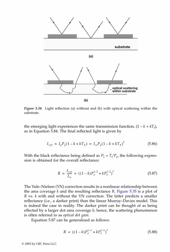
Chapter five: Device characterization 349
the emerging light experiences the same transmission function, (1 – k + kTk),as in Equation 5.84. The final reflected light is given by
(5.86)
With the black reflectance being defined as Pk = Tk2Pp, the following expres-
sion is obtained for the overall reflectance:
(5.87)
The Yule–Nielsen (YN) correction results in a nonlinear relationship betweenthe area coverage k and the resulting reflectance R. Figure 5.35 is a plot ofR vs. k with and without the YN correction. The latter predicts a smallerreflectance (i.e., a darker print) than the linear Murray–Davies model. Thisis indeed the case in reality. The darker print can be thought of as beingeffected by a larger dot area coverage k; hence, the scattering phenomenonis often referred to as optical dot gain.
Equation 5.87 can be generalized as follows:
(5.88)
Figure 5.34 Light reflection (a) without and (b) with optical scattering within thesubstrate.
Ireft IpPp 1 k– kTK+( ) IinPp 1 k– kTK+( )2= =
RIreft
Iin-------- 1 k–( )Pp
1 2⁄ kPk1 2⁄+( )2
= =
R 1 k–( )Pp1 n⁄ kPk
1 n⁄+( )n=
-ColorBook Page 349 Wednesday, November 13, 2002 10:55 AM
© 2003 by CRC Press LLC
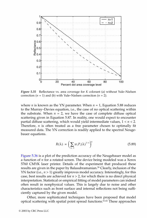
350 Digital Color Imaging Handbook
where n is known as the YN parameter. When n = 1, Equation 5.88 reducesto the Murray–Davies equation, i.e., the case of no optical scattering withinthe substrate. When n = 2, we have the case of complete diffuse opticalscattering given in Equation 5.87. In reality, one would expect to encounterpartial diffuse scattering, which would yield intermediate values, 1 < n < 2.Therefore, n is often treated as a free parameter chosen to optimally fitmeasured data. The YN correction is readily applied to the spectral Neuge-bauer equations.
(5.89)
Figure 5.36 is a plot of the prediction accuracy of the Neugebauer model asa function of n for a rotated screen. The device being modeled was a Xerox5760 CMYK laser printer. Details of the experiment that produced theseresults are given in the paper by Balasubramanian.59 Clearly, inclusion of theYN factor (i.e., n > 1) greatly improves model accuracy. Interestingly, for thiscase, best results are achieved for n > 2, for which there is no direct physicalinterpretation. Statistical or empirical fitting of model parameters can indeedoften result in nonphysical values. This is largely due to noise and othercharacteristics such as front surface and internal reflections not being suffi-ciently captured by the given model.
Other, more sophisticated techniques have been proposed that modeloptical scattering with spatial point spread functions.61,62 These approaches
0 20 40 60 80 1000
0.1
0.2
0.3
0.4
0.5
0.6
0.7
0.8
0.9
1
Percent dot area coverage level
Ref
lect
ance
n=1n=2
Figure 5.35 Reflectance vs. area coverage for K colorant (a) without Yule–Nielsencorrection (n = 1) and (b) with Yule–Nielsen correction (n = 2).
R λ( ) wiPi λ( )1 n⁄
i S∈∑
n=
-ColorBook Page 350 Wednesday, November 13, 2002 10:55 AM
© 2003 by CRC Press LLC
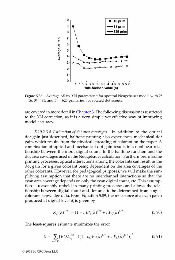
Chapter five: Device characterization 351
are covered in more detail in Chapter 3. The following discussion is restrictedto the YN correction, as it is a very simple yet effective way of improvingmodel accuracy.
5.10.2.3.4 Estimation of dot area coverages. In addition to the opticaldot gain just described, halftone printing also experiences mechanical dotgain, which results from the physical spreading of colorant on the paper. Acombination of optical and mechanical dot gain results in a nonlinear rela-tionship between the input digital counts to the halftone function and thedot area coverages used in the Neugebauer calculation. Furthermore, in someprinting processes, optical interactions among the colorants can result in thedot gain for a given colorant being dependent on the area coverages of theother colorants. However, for pedagogical purposes, we will make the sim-plifying assumption that there are no interchannel interactions so that thecyan area coverage depends on only the cyan digital count, etc. This assump-tion is reasonably upheld in many printing processes and allows the rela-tionship between digital count and dot area to be determined from single-colorant stepwedge data. From Equation 5.89, the reflectance of a cyan patchproduced at digital level dj is given by
(5.90)
The least-squares estimate minimizes the error
(5.91)
Yule-Nielsen value (n)
Ave
rag
e ∆E
*ab
0
1
2
3
4
5
6
7
8
9
10
1 1.5 2 2.5 3 3.5 4 4.5 5 5.5 6
16 prim
81 prim
625 prim
Figure 5.36 Average ∆E vs. YN parameter n for spectral Neugebauer model with 24
= 16, 34 = 81, and 54 = 625 primaries, for rotated dot screen.
RCiλ( )1 n⁄ 1 cj–( )Pp λ( )1 n⁄ cjPC λ( )1 n⁄+=
E R λ( )Cj
1 n⁄ 1 cj–( )PP λ( )1 n⁄ cjPC λ( )1 n⁄+( )–[ ]2
λ V∈∑=
-ColorBook Page 351 Wednesday, November 13, 2002 10:55 AM
© 2003 by CRC Press LLC
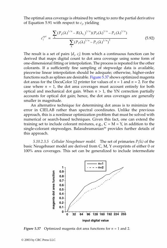
352 Digital Color Imaging Handbook
The optimal area coverage is obtained by setting to zero the partial derivativeof Equation 5.91 with respect to cj, yielding
(5.92)
The result is a set of pairs {dj, cj} from which a continuous function can bederived that maps digital count to dot area coverage using some form ofone-dimensional fitting or interpolation. The process is repeated for the othercolorants. If a sufficiently fine sampling of stepwedge data is available,piecewise linear interpolation should be adequate; otherwise, higher-orderfunctions such as splines are desirable. Figure 5.37 shows optimized magentadot areas for the DocuColor 12 printer for values of n = 1 and n = 2. For thecase where n = 1, the dot area coverages must account entirely for bothoptical and mechanical dot gain. When n > 1, the YN correction partiallyaccounts for optical dot gain; hence, the dot area coverages are generallysmaller in magnitude.
An alternative technique for determining dot areas is to minimize theerror in CIELAB rather than spectral coordinates. Unlike the previousapproach, this is a nonlinear optimization problem that must be solved withnumerical or search-based techniques. Given this fact, one can extend thetraining set to include colorant mixtures, e.g., C = M = Y, in addition to thesingle-colorant stepwedges. Balasubramanian59 provides further details ofthis approach.
5.10.2.3.5 Cellular Neugebauer model. The set of primaries Pi(λ) of thebasic Neugebauer model are derived from C, M, Y overprints of either 0 or100% area coverages. This set can be generalized to include intermediate
cjopt
Pp λ( )1 n⁄ R λc j( )1 n⁄–( ) PP λ( )1 n⁄ PC λ( )1 n⁄–( )
λ∑
PP λ( )1 n⁄ PC λ( )1 n⁄–( )2
λ∑
-------------------------------------------------------------------------------------------------------------------=
input digital value
10.9
0.80.70.60.50.40.3
0.20.1
00 32 64 96 128 160 224 255192
mag
enta
do
t ar
ea f
un
ctio
n
n=1n=2
Figure 5.37 Optimized magenta dot area functions for n = 1 and 2.
-ColorBook Page 352 Wednesday, November 13, 2002 10:55 AM
© 2003 by CRC Press LLC
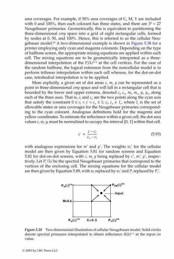
Chapter five: Device characterization 353
area coverages. For example, if 50% area coverages of C, M, Y are includedwith 0 and 100%, then each colorant has three states, and there are 33 = 27Neugebauer primaries. Geometrically, this is equivalent to partitioning thethree-dimensional cmy space into a grid of eight rectangular cells, formedby nodes at 0, 50, and 100%. Hence, this is referred to as the cellular Neu-gebauer model.63 A two-dimensional example is shown in Figure 5.38 for aprinter employing only cyan and magenta colorants. Depending on the typeof halftone screen, the appropriate mixing equations are applied within eachcell. The mixing equations are to be geometrically interpreted as a three-dimensional interpolation of the Pi(λ)1/n at the cell vertices. For the case ofthe random halftone, the logical extension from the noncellular model is toperform trilinear interpolation within each cell whereas, for the dot-on-dotcase, tetrahedral interpolation is to be applied.
More explicitly, a given set of dot areas c, m, y can be represented as apoint in three-dimensional cmy space and will fall in a rectangular cell that isbounded by the lower and upper extrema, denoted cl, cu, ml, mu, yl, yu, alongeach of the three axes. That is, cl and cu are the two points along the cyan axisthat satisfy the constraint 0 ≤ cl < c < cu ≤ 1; cl, cu ∈ Ic, where Ic is the set ofallowable states or area coverages for the Neugebauer primaries correspond-ing to the cyan colorant. Analogous definitions hold for the magenta andyellow coordinates. To estimate the reflectance within a given cell, the dot areavalues c, m, y, must be normalized to occupy the interval [0, 1] within that cell.
(5.93)
with analogous expressions for m’ and y’. The weights wi’ for the cellularmodel are then given by Equation 5.81 for random screens and Equation5.82 for dot-on-dot screens, with c, m, y being replaced by c’, m’, y’, respec-tively. Let Pi’(λ) be the spectral Neugebauer primaries that correspond to thevertices of the enclosing cell. The mixing equations for the cellular modelare then given by Equation 5.89, with wi replaced by wi’ and Pi replaced by Pi’.
Input
Pw(λ)1/n P C(λ)1/n
PM(λ)1/n PCM(λ)1/n
C=0.5
M=0.5
Figure 5.38 Two-dimensional illustration of cellular Neugebauer model. Solid circlesdenote spectral primaries interpolated to obtain reflectance R(λ)1/n at the input cmvalue.
c, c cl–cu cl–--------------=
-ColorBook Page 353 Wednesday, November 13, 2002 10:55 AM
© 2003 by CRC Press LLC
354 Digital Color Imaging Handbook
Note that the cellular equations physically model a halftoning processwherein each colorant can produce M > 2 concentration levels. For binaryprinters, the justification for using a cellular model is empirical rather thanphysical; the finer cellular subdivision of cmy space affords finer interpola-tion of measured data, hence yielding greater accuracy.
Figure 5.36 compares the accuracy of the noncellular model for a CMYKprinter with cellular versions employing 34 = 81 and 54 = 625 primaries. Asthe number of cells increases, the model accuracy improves significantly. Atthe same time, the dependence on the YN factor decreases. This is to beexpected, as the cellular model marks a transition from a model-based to anempirical approach and hence would be less sensitive to model parameters.
5.10.2.3.6 Spectral regression of the Neugebauer primaries. Thus far, theprimaries Pi(λ) in Equation 5.89 are considered as fixed parameters that aredirectly measured. An alternative is to treat these quantities as free variablesthat can be optimized via regression on a training set of spectral reflectancedata. This technique will be described next for the case of a noncellular CMYmodel employing rotated screens. (Extension to the cellular case, N colorants,or dot-on-dot screen is straightforward). It is assumed that the optimal nfactor and dot area coverages have been derived using the aforementionedtechniques. To formulate the regression problem, it is convenient to expressthe Neugebauer equations in matrix-vector form. Consider each spectralmeasurement as an L-vector. Collect the YN modified spectral reflectancesR(λ)1/n of T training samples into a T × L matrix R. Similarly, collect the YNmodified Neugebauer primaries Pi(λ)1/n into an 8 × L matrix P. Finally, gen-erate a T × 8 weight matrix W whose element wij is the area coverage of thejth Neugebauer primary for the ith training sample. Equation 5.89 can thenbe rewritten as
R = W · P (5.94)
From Appendix 5.A, the least squares solution for P is given by
Popt = (WtW–1)WtR (5.95)
The terms in P are raised to the power n to obtain optimized primary reflec-tances. It must be emphasized that the choice of CMY samples in the trainingset T is crucial in determining the condition or rank of matrix W. Namely, toensure sufficient rank, the samples should be chosen so that there are no nullcolumns in W. A simple way to assure this is to pick a regular three-dimen-sional grid of training samples. Also, note that the foregoing analysis is basedon a particular choice of n and the dot area coverage functions. The processcan be iteratively repeated by rederiving n and the dot areas correspondingto the newly optimized primaries, and then repeating the regression step.Experiments by the author have shown that more than two iterations do notgenerally yield significant improvements in model accuracy.59
-ColorBook Page 354 Wednesday, November 13, 2002 10:55 AM
© 2003 by CRC Press LLC
Chapter five: Device characterization 355
5.10.2.3.7 Overall model optimization. The following procedure maybe used to optimize the various parameters of the Neugebauer model for aCMY printer:
• Select the resolution of the cellular Neugebauer model. In the au-thor’s experience, three levels (i.e., two cells) per colorant offers anacceptable trade-off between accuracy and number of samples re-quired. Generate CMY combinations corresponding to the cell nodes(i.e., the Neugebauer primaries).
• Select the resolution of C, M, Y stepwedges to generate dot areafunctions. In the author’s experience, a minimum of 16 samples percolorant is usually adequate.
• Select an additional set of CMY mixtures to test and refine the model.One possibility is to use an N × N × N grid of CMY combinationsthat does not coincide with the Neugebauer primaries.
• Combine the above CMY samples into a characterization target. (Asan alternative to designing a custom target, the standard IT8.7/3printer characterization target described in Section 5.3 can be used,as it contains the patches necessary to derive and test the Neugebauermodel.) Print the target and obtain spectral measurements.
• For a fixed value of n (e.g., n = 1), use Equation 5.92 to generateestimates of dot area coverages for the stepwedge samples. Interpo-late or fit the data to create functions that map digital count to dotarea coverages. With 16 or more samples per stepwedge, piecewiselinear interpolation should produce adequate accuracy.
• Evaluate the accuracy of the model in predicting the stepwedge data.This is accomplished by computing a ∆E metric between model pre-dictions with actual measurements.
• Optimize the model with respect to n by repeating the previous twosteps for several n values in some nominal range (e.g., 1 < n < 7) andselecting the n that produces the minimum ∆E.
• Select a mixing model depending on the type of halftone screen (e.g.,Demichel vs. dot-on-dot).
• If the dot-on-dot model is chosen, find the optimal blending param-eter α in Equation 5.83 by iterating through different values of α,computing ∆E for the model’s prediction of mixed color samples fromthe test set, and selecting α that minimizes the ∆E.
• If spectral regression of the primaries is desired, select a set of mixedcolor samples from the test set, and use Equation 5.95 to computeoptimal primaries Pi(λ).
Figure 5.39 summarizes the steps in the application of the Neugebauermodel. Accuracy of the model must be evaluated on an independent setof CMY samples. If the prediction error is within the variability of theprinter, the model is considered to be a satisfactory representation of thereal printer.
-ColorBook Page 355 Wednesday, November 13, 2002 10:55 AM
© 2003 by CRC Press LLC
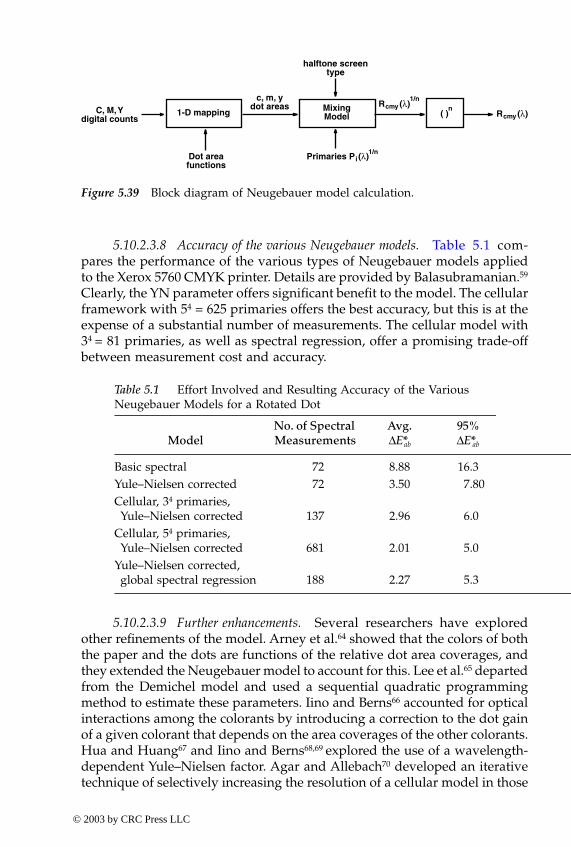
356 Digital Color Imaging Handbook
5.10.2.3.8 Accuracy of the various Neugebauer models. Table 5.1 com-pares the performance of the various types of Neugebauer models appliedto the Xerox 5760 CMYK printer. Details are provided by Balasubramanian.59
Clearly, the YN parameter offers significant benefit to the model. The cellularframework with 54 = 625 primaries offers the best accuracy, but this is at theexpense of a substantial number of measurements. The cellular model with34 = 81 primaries, as well as spectral regression, offer a promising trade-offbetween measurement cost and accuracy.
5.10.2.3.9 Further enhancements. Several researchers have exploredother refinements of the model. Arney et al.64 showed that the colors of boththe paper and the dots are functions of the relative dot area coverages, andthey extended the Neugebauer model to account for this. Lee et al.65 departedfrom the Demichel model and used a sequential quadratic programmingmethod to estimate these parameters. Iino and Berns66 accounted for opticalinteractions among the colorants by introducing a correction to the dot gainof a given colorant that depends on the area coverages of the other colorants.Hua and Huang67 and Iino and Berns68,69 explored the use of a wavelength-dependent Yule–Nielsen factor. Agar and Allebach70 developed an iterativetechnique of selectively increasing the resolution of a cellular model in those
Table 5.1 Effort Involved and Resulting Accuracy of the Various Neugebauer Models for a Rotated Dot
ModelNo. of Spectral Measurements
Avg.∆E*ab
95% ∆E*ab
Basic spectral 72 8.88 16.3Yule–Nielsen corrected 72 3.50 7.80Cellular, 34 primaries,
Yule–Nielsen corrected 137 2.96 6.0Cellular, 54 primaries,
Yule–Nielsen corrected 681 2.01 5.0Yule–Nielsen corrected, global spectral regression 188 2.27 5.3
C, M, Ydigital counts
Dot areafunctions
halftone screentype
c, m, ydot areas
1-D mapping MixingModel
Primaries P (λ)i1/n
cmyR (λ)1/n
( )n
cmyR (λ)
Figure 5.39 Block diagram of Neugebauer model calculation.
-ColorBook Page 356 Wednesday, November 13, 2002 10:55 AM
© 2003 by CRC Press LLC
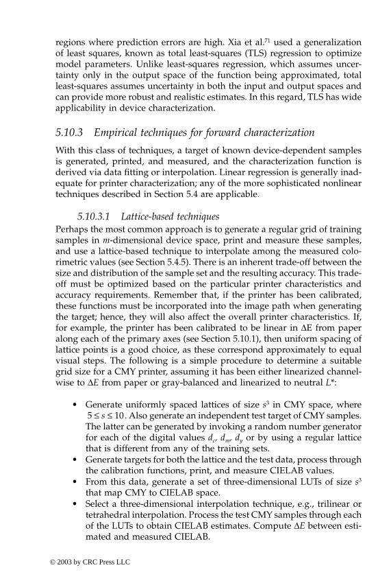
Chapter five: Device characterization 357
regions where prediction errors are high. Xia et al.71 used a generalizationof least squares, known as total least-squares (TLS) regression to optimizemodel parameters. Unlike least-squares regression, which assumes uncer-tainty only in the output space of the function being approximated, totalleast-squares assumes uncertainty in both the input and output spaces andcan provide more robust and realistic estimates. In this regard, TLS has wideapplicability in device characterization.
5.10.3 Empirical techniques for forward characterization
With this class of techniques, a target of known device-dependent samplesis generated, printed, and measured, and the characterization function isderived via data fitting or interpolation. Linear regression is generally inad-equate for printer characterization; any of the more sophisticated nonlineartechniques described in Section 5.4 are applicable.
5.10.3.1 Lattice-based techniquesPerhaps the most common approach is to generate a regular grid of trainingsamples in m-dimensional device space, print and measure these samples,and use a lattice-based technique to interpolate among the measured colo-rimetric values (see Section 5.4.5). There is an inherent trade-off between thesize and distribution of the sample set and the resulting accuracy. This trade-off must be optimized based on the particular printer characteristics andaccuracy requirements. Remember that, if the printer has been calibrated,these functions must be incorporated into the image path when generatingthe target; hence, they will also affect the overall printer characteristics. If,for example, the printer has been calibrated to be linear in ∆E from paperalong each of the primary axes (see Section 5.10.1), then uniform spacing oflattice points is a good choice, as these correspond approximately to equalvisual steps. The following is a simple procedure to determine a suitablegrid size for a CMY printer, assuming it has been either linearized channel-wise to ∆E from paper or gray-balanced and linearized to neutral L*:
• Generate uniformly spaced lattices of size s3 in CMY space, where. Also generate an independent test target of CMY samples.
The latter can be generated by invoking a random number generatorfor each of the digital values dc, dm, dy or by using a regular latticethat is different from any of the training sets.
• Generate targets for both the lattice and the test data, process throughthe calibration functions, print, and measure CIELAB values.
• From this data, generate a set of three-dimensional LUTs of size s3
that map CMY to CIELAB space.• Select a three-dimensional interpolation technique, e.g., trilinear or
tetrahedral interpolation. Process the test CMY samples through eachof the LUTs to obtain CIELAB estimates. Compute ∆E between esti-mated and measured CIELAB.
5 s 10≤ ≤
-ColorBook Page 357 Wednesday, November 13, 2002 10:55 AM
© 2003 by CRC Press LLC
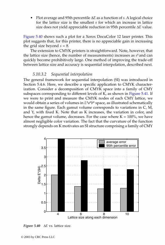
358 Digital Color Imaging Handbook
• Plot average and 95th percentile ∆E as a function of s. A logical choicefor the lattice size is the smallest s for which an increase in latticesize does not yield appreciable reduction in 95th percentile ∆E value.
Figure 5.40 shows such a plot for a Xerox DocuColor 12 laser printer. Thisplot suggests that, for this printer, there is no appreciable gain in increasingthe grid size beyond s = 8.
The extension to CMYK printers is straightforward. Note, however, thatthe lattice size (hence, the number of measurements) increases as s4 and canquickly become prohibitively large. One method of improving the trade-offbetween lattice size and accuracy is sequential interpolation, described next.
5.10.3.2 Sequential interpolationThe general framework for sequential interpolation (SI) was introduced inSection 5.4.6. Here, we describe a specific application to CMYK character-ization. Consider a decomposition of CMYK space into a family of CMYsubspaces corresponding to different levels of K, as shown in Figure 5.41. Ifwe were to print and measure the CMYK nodes of each CMY lattice, wewould obtain a series of volumes in L*a*b* space, as illustrated schematicallyin the same figure. Each gamut volume corresponds to variations in C, M,and Y, with fixed K. Note that as K increases, the variation in color, andhence the gamut volume, decreases. For the case where K = 100%, we havealmost negligible color variation. The fact that the curvature of the functionstrongly depends on K motivates an SI structure comprising a family of CMY
4 6 8 100
0.5
1
1.5
2
2.5
3
3.5
4
Lattice size along each dimension
Del
ta E
*(94
)
average error95th percentile error
Figure 5.40 ∆E vs. lattice size.
-ColorBook Page 358 Wednesday, November 13, 2002 10:55 AM
© 2003 by CRC Press LLC
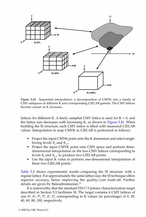
Chapter five: Device characterization 359
lattices for different K. A finely sampled CMY lattice is used for K = 0, andthe lattice size decreases with increasing K, as shown in Figure 5.41. Whenbuilding the SI structure, each CMY lattice is filled with measured CIELABvalues. Interpolation to map CMYK to CIELAB is performed as follows:
• Project the input CMYK point onto the K dimension and select neigh-boring levels Kj and Kj+1.
• Project the input CMYK point onto CMY space and perform three-dimensional interpolation on the two CMY lattices corresponding tolevels Kj and Kj+1 to produce two CIELAB points.
• Use the input K value to perform one-dimensional interpolation ofthese two CIELAB points.
Table 5.2 shows experimental results comparing the SI structure with aregular lattice. For approximately the same lattice size, the SI technique offerssuperior accuracy, hence improving the quality/cost trade-off. Furtherdetails are given by Balasubramanian.72
It is noteworthy that the standard IT8.7/3 printer characterization targetdescribed in Section 5.3 facilitates SI. The target contains 6 CMY lattices ofsize 63, 63, 53, 53, 43, 23, corresponding to K values (in percentage) of 0, 20,40, 60, 80, 100, respectively.
C*
L*
Y
M
C K=100%
Y
M
C K=50%
M
Y
C K=0%
Figure 5.41 Sequential interpolation: a decomposition of CMYK into a family ofCMY subspaces at different K and corresponding CIELAB gamuts. The CMY latticesbecome coarser as K increases.
-ColorBook Page 359 Wednesday, November 13, 2002 10:55 AM
© 2003 by CRC Press LLC
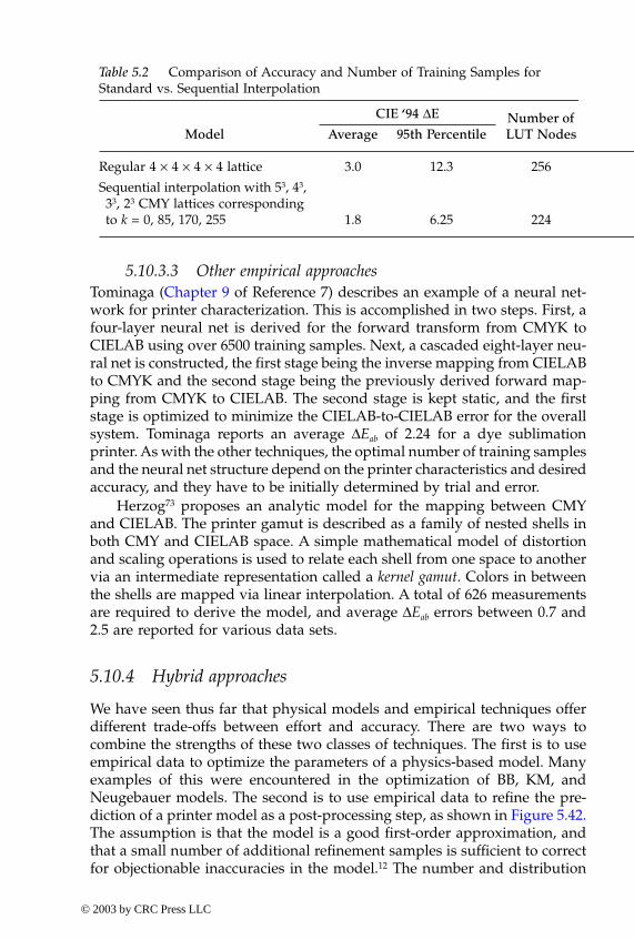
360 Digital Color Imaging Handbook
5.10.3.3 Other empirical approachesTominaga (Chapter 9 of Reference 7) describes an example of a neural net-work for printer characterization. This is accomplished in two steps. First, afour-layer neural net is derived for the forward transform from CMYK toCIELAB using over 6500 training samples. Next, a cascaded eight-layer neu-ral net is constructed, the first stage being the inverse mapping from CIELABto CMYK and the second stage being the previously derived forward map-ping from CMYK to CIELAB. The second stage is kept static, and the firststage is optimized to minimize the CIELAB-to-CIELAB error for the overallsystem. Tominaga reports an average ∆Eab of 2.24 for a dye sublimationprinter. As with the other techniques, the optimal number of training samplesand the neural net structure depend on the printer characteristics and desiredaccuracy, and they have to be initially determined by trial and error.
Herzog73 proposes an analytic model for the mapping between CMYand CIELAB. The printer gamut is described as a family of nested shells inboth CMY and CIELAB space. A simple mathematical model of distortionand scaling operations is used to relate each shell from one space to anothervia an intermediate representation called a kernel gamut. Colors in betweenthe shells are mapped via linear interpolation. A total of 626 measurementsare required to derive the model, and average ∆Eab errors between 0.7 and2.5 are reported for various data sets.
5.10.4 Hybrid approaches
We have seen thus far that physical models and empirical techniques offerdifferent trade-offs between effort and accuracy. There are two ways tocombine the strengths of these two classes of techniques. The first is to useempirical data to optimize the parameters of a physics-based model. Manyexamples of this were encountered in the optimization of BB, KM, andNeugebauer models. The second is to use empirical data to refine the pre-diction of a printer model as a post-processing step, as shown in Figure 5.42.The assumption is that the model is a good first-order approximation, andthat a small number of additional refinement samples is sufficient to correctfor objectionable inaccuracies in the model.12 The number and distribution
Table 5.2 Comparison of Accuracy and Number of Training Samples for Standard vs. Sequential Interpolation
Model
CIE ‘94 ∆E Number of LUT NodesAverage 95th Percentile
Regular 4 × 4 × 4 × 4 lattice 3.0 12.3 256
Sequential interpolation with 53, 43, 33, 23 CMY lattices corresponding to k = 0, 85, 170, 255 1.8 6.25 224
-ColorBook Page 360 Wednesday, November 13, 2002 10:55 AM
© 2003 by CRC Press LLC
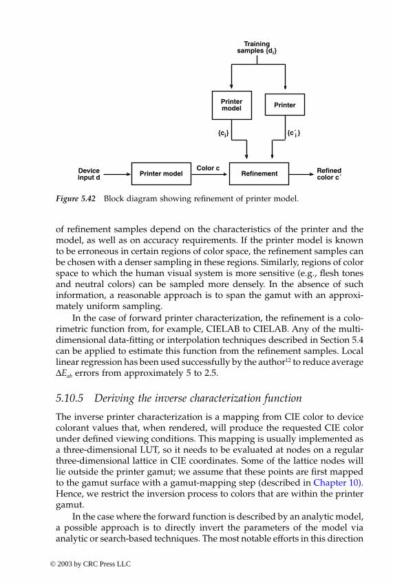
Chapter five: Device characterization 361
of refinement samples depend on the characteristics of the printer and themodel, as well as on accuracy requirements. If the printer model is knownto be erroneous in certain regions of color space, the refinement samples canbe chosen with a denser sampling in these regions. Similarly, regions of colorspace to which the human visual system is more sensitive (e.g., flesh tonesand neutral colors) can be sampled more densely. In the absence of suchinformation, a reasonable approach is to span the gamut with an approxi-mately uniform sampling.
In the case of forward printer characterization, the refinement is a colo-rimetric function from, for example, CIELAB to CIELAB. Any of the multi-dimensional data-fitting or interpolation techniques described in Section 5.4can be applied to estimate this function from the refinement samples. Locallinear regression has been used successfully by the author12 to reduce average∆Eab errors from approximately 5 to 2.5.
5.10.5 Deriving the inverse characterization function
The inverse printer characterization is a mapping from CIE color to devicecolorant values that, when rendered, will produce the requested CIE colorunder defined viewing conditions. This mapping is usually implemented asa three-dimensional LUT, so it needs to be evaluated at nodes on a regularthree-dimensional lattice in CIE coordinates. Some of the lattice nodes willlie outside the printer gamut; we assume that these points are first mappedto the gamut surface with a gamut-mapping step (described in Chapter 10).Hence, we restrict the inversion process to colors that are within the printergamut.
In the case where the forward function is described by an analytic model,a possible approach is to directly invert the parameters of the model viaanalytic or search-based techniques. The most notable efforts in this direction
Deviceinput d Refinement Refined
color c´Printer modelColor c
Printermodel Printer
Trainingsamples {d }i
{c }i {c´ }i
Figure 5.42 Block diagram showing refinement of printer model.
-ColorBook Page 361 Wednesday, November 13, 2002 10:55 AM
© 2003 by CRC Press LLC
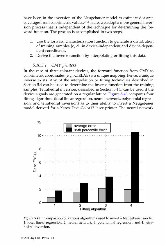
362 Digital Color Imaging Handbook
have been in the inversion of the Neugebauer model to estimate dot areacoverages from colorimetric values.74,75 Here, we adopt a more general inver-sion process that is independent of the technique for determining the for-ward function. The process is accomplished in two steps.
1. Use the forward characterization function to generate a distributionof training samples {ci, di} in device-independent and device-depen-dent coordinates.
2. Derive the inverse function by interpolating or fitting this data.
5.10.5.1 CMY printersIn the case of three-colorant devices, the forward function from CMY tocolorimetric coordinates (e.g., CIELAB) is a unique mapping; hence, a uniqueinverse exists. Any of the interpolation or fitting techniques described inSection 5.4 can be used to determine the inverse function from the trainingsamples. Tetrahedral inversion, described in Section 5.4.5, can be used if thedevice signals are generated on a regular lattice. Figure 5.43 compares fourfitting algorithms (local linear regression, neural network, polynomial regres-sion, and tetrahedral inversion) as to their ability to invert a Neugebauermodel derived for a Xerox DocuColor12 laser printer. The neural network
1 2 3 40
2
4
6
8
10
12
Fitting algorithm
Del
ta E
*(94
)
average error95th percentile error
Figure 5.43 Comparison of various algorithms used to invert a Neugebauer model:1. local linear regression, 2. neural network, 3. polynomial regression, and 4. tetra-hedral inversion.
-ColorBook Page 362 Wednesday, November 13, 2002 10:55 AM
© 2003 by CRC Press LLC
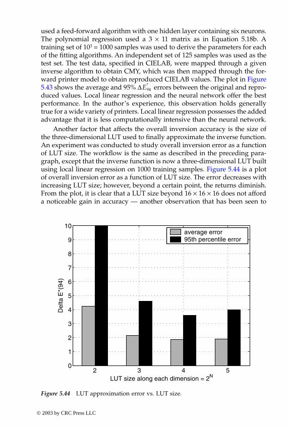
Chapter five: Device characterization 363
used a feed-forward algorithm with one hidden layer containing six neurons.The polynomial regression used a 3 × 11 matrix as in Equation 5.18b. Atraining set of 103 = 1000 samples was used to derive the parameters for eachof the fitting algorithms. An independent set of 125 samples was used as thetest set. The test data, specified in CIELAB, were mapped through a giveninverse algorithm to obtain CMY, which was then mapped through the for-ward printer model to obtain reproduced CIELAB values. The plot in Figure5.43 shows the average and 95% ∆ errors between the original and repro-duced values. Local linear regression and the neural network offer the bestperformance. In the author’s experience, this observation holds generallytrue for a wide variety of printers. Local linear regression possesses the addedadvantage that it is less computationally intensive than the neural network.
Another factor that affects the overall inversion accuracy is the size ofthe three-dimensional LUT used to finally approximate the inverse function.An experiment was conducted to study overall inversion error as a functionof LUT size. The workflow is the same as described in the preceding para-graph, except that the inverse function is now a three-dimensional LUT builtusing local linear regression on 1000 training samples. Figure 5.44 is a plotof overall inversion error as a function of LUT size. The error decreases withincreasing LUT size; however, beyond a certain point, the returns diminish.From the plot, it is clear that a LUT size beyond 16 × 16 × 16 does not afforda noticeable gain in accuracy — another observation that has been seen to
E94*
2 3 4 50
1
2
3
4
5
6
7
8
9
10
LUT size along each dimension = 2N
Del
ta E
*(94
)
average error95th percentile error
Figure 5.44 LUT approximation error vs. LUT size.
-ColorBook Page 363 Wednesday, November 13, 2002 10:55 AM
© 2003 by CRC Press LLC
364 Digital Color Imaging Handbook
hold true for a wide variety of printers. Note that the relative spacing ofnodes along each dimension can also affect LUT accuracy. In this experiment,the nodes were spaced uniformly, because the input space, CIELAB, in whichthe LUT was built, is approximately visually uniform.
5.10.5.2 CMYK printers
Although, in principle, the three C, M, and Y colorants suffice to produceall perceivable hues, very often, a fourth black (K) colorant is used for severalreasons. First, the K colorant is usually considerably less expensive than C,M, and Y, and it can thus be used in lieu of CMY mixtures to render darkneutrals and shadows. Second, the addition of K can result in an increase ingamut in the dark regions of color space in comparison to what is achievableusing only CMY mixtures. Third, the use of K can help reduce the totalamount of colorant required to produce a given color, a feature that is criticalin certain technologies such as inkjet printing.
In the context of device characterization, the K colorant introducesredundancy into the forward transform, as a large (in principle, infinite)number of CMYK combinations can result in the same colorimetric measure-ment. This results in the inverse function being ill posed, and additionalconstraints are required to generate a unique CMYK combination for eachinput CIE color. Some common methods of deriving the constrained inverseare presented next.
5.10.5.2.1 Inversion based on K addition, undercolor removal, and graycomponent replacement. The processes of black (K) addition, undercolorremoval (UCR), and gray component replacement (GCR) trace their originsto the graphic arts printing industry.50 Together, they define a unique trans-form from a set of canonical CMY primaries to the CMYK signals for thegiven printer. Geometrically, the transform generates a three-dimensionalmanifold within the four-dimensional CMYK space, with the property thatevery CMYK combination within the manifold results in a unique colori-metric response. Once this transform is established, the inversion can becarried out on the canonical CMY device as described in Section 5.10.5.1.Figure 5.45 shows the derivation and application of the inverse functionfor a CMYK printer. The two functions in Figure 5.45b are usually concat-enated into a composite inverse transform from CIE to CMYK signals.Recall that the printer is assumed to have been calibrated, so the CMYKsignals resulting form the inversion process are finally processed throughthe calibration functions prior to printing. In some implementations, thecalibration is concatenated with the characterization or stored in the sameprofile.
There are numerous methods for designing K addition, UCR, and GCRfunctions. They are usually chosen for an optimal trade-off among factorssuch as gamut volume, colorant area coverage, and smoothness of transitionsfrom neutral to non-neutral colors. The trade-off is usually carried out
-ColorBook Page 364 Wednesday, November 13, 2002 10:55 AM
© 2003 by CRC Press LLC
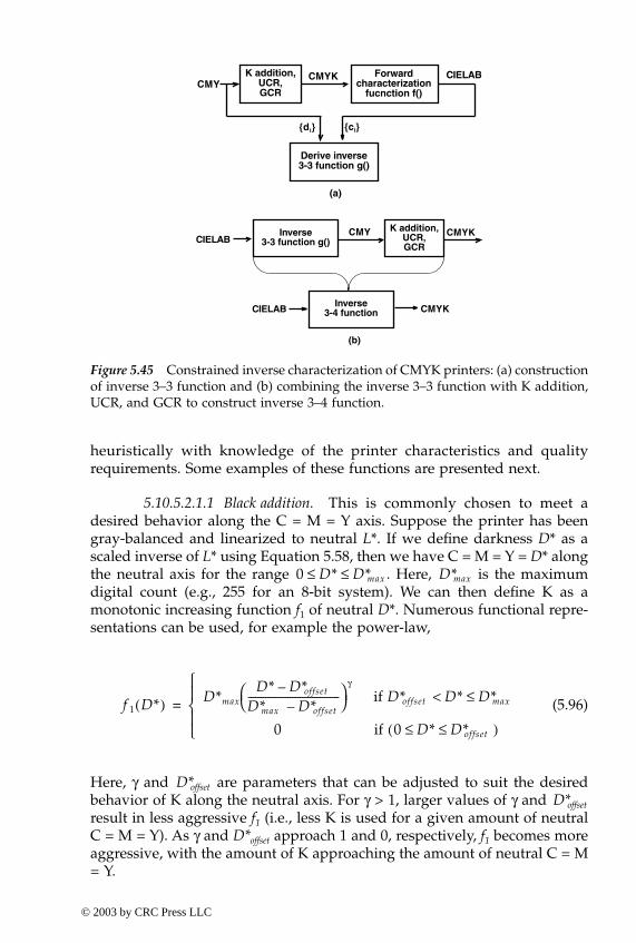
Chapter five: Device characterization 365
heuristically with knowledge of the printer characteristics and qualityrequirements. Some examples of these functions are presented next.
5.10.5.2.1.1 Black addition. This is commonly chosen to meet adesired behavior along the C = M = Y axis. Suppose the printer has beengray-balanced and linearized to neutral L*. If we define darkness D* as ascaled inverse of L* using Equation 5.58, then we have C = M = Y = D* alongthe neutral axis for the range . Here, is the maximumdigital count (e.g., 255 for an 8-bit system). We can then define K as amonotonic increasing function f1 of neutral D*. Numerous functional repre-sentations can be used, for example the power-law,
(5.96)
Here, γ and D*offset are parameters that can be adjusted to suit the desiredbehavior of K along the neutral axis. For γ > 1, larger values of γ and D*offset
result in less aggressive f1 (i.e., less K is used for a given amount of neutralC = M = Y). As γ and D*offset approach 1 and 0, respectively, f1 becomes moreaggressive, with the amount of K approaching the amount of neutral C = M= Y.
{di} {ci}
CIELABCMY
CMYK Forwardcharacterization
fucnction f()
K addition,UCR,GCR
Derive inverse3-3 function g()
(a)
CIELAB CMY CMYKK addition,
UCR,GCR
(b)
Inverse3-3 function g()
Inverse3-4 functionCIELAB CMYK
Figure 5.45 Constrained inverse characterization of CMYK printers: (a) constructionof inverse 3–3 function and (b) combining the inverse 3–3 function with K addition,UCR, and GCR to construct inverse 3–4 function.
0 D* D*max≤ ≤ D*max
f 1 D*( ) D*maxD* D*offset–
D*max D*offset–-------------------------------------
γ
if D*offset D* D*max≤<
0 if 0 D* D*offset≤ ≤( )
=
-ColorBook Page 365 Wednesday, November 13, 2002 10:55 AM
© 2003 by CRC Press LLC
366 Digital Color Imaging Handbook
5.10.5.2.1.2 Undercolor removal.
This function describes theamount of reduction in CMY primaries to compensate for the K addition. Itis also derived with attention to the neutral axis. A simple form of CMYreduction is given by
C’ = C –
f
2
(
D*
) (5.97)
with analogous expressions for M and Y. Again, we are abounded withnumerous strategies for
f
2
(D*).
One approach is based on the rationale thatthe CMY reduction should be proportional to the amount of K addition,
(5.98)
The case where
a
= 1 (i.e., CMY subtraction equals K addition) is oftenreferred to as 100% UCR.
A more sophisticated approach is to derive
f
2
to colorimetrically com-pensate for the K addition. This can be performed as follows. For a givenneutral input C = M = Y sample, the resulting
L
* and hence
D
* that wouldbe produced by printing this sample can be predicted via the forward char-acterization function. The amount of K associated with this input C = M =Y is given by
f
1
()
.
We can now derive the new smaller amounts, C’ = M’ =Y’, which produce the same
D
* when combined with the given K. This stepis achieved by combining different C = M = Y levels with the given K, runningthrough the forward transform, and picking the combination that producesthe desired
D
*. Finally,
f
2
is the difference between the original C = M = Yand final C’= M’= Y’.
A key factor to be considered in choosing black addition and UCRparameters is the total area coverage (TAC) that is permissible for the givendevice, especially in the dark portions of the gamut. For many CMYK print-ers, TACs near 400% will result in defects (e.g., ink bleeding in inkjet printersor improper toner fusing and flaking in xerographic printers). Hence, anappropriate limit must be placed on TAC, and this in turn affects the Kaddition and UCR parameters. If the colorimetric approach described in thepreceding paragraph is adopted, accuracy will likely be sacrificed towardthe dark end of the gamut due to TAC limits.
5.10.5.2.1.3 Gray component replacement.
Thus far, K addition andUCR have been defined for neutral samples C = M = Y. GCR is a generali-zation of these functions for the entire gamut of CMY combinations. Afundamental assumption is that the gray component of an arbitrary CMYcombination is given by the minimum of C, M, Y. This gray component canthen be used as input to the K addition and UCR functions.
X = min(C,M,Y)
K =
f
1
(X)
f 2 D*( ) af 1 D*( )= , 0 a 1£ £
05 Page 366 Monday, November 18, 2002 8:25 AM
© 2003 by CRC Press LLC
Chapter five: Device characterization 367
C’ = C – f2(X)
M’ = M – f2(X)
Y’ = Y – f2(X) (5.99)
Clearly, one can conceive numerous enhancements to this simple model. TheCMY subtraction can be performed in other spaces such as optical density.This can be accomplished in the current framework by applying a transformto the chosen space before CMY subtraction and applying the inverse trans-form after subtraction. Second, functions f1 and f2 can be multidimensionalfunctions that depend on more than just the minimum of C, M, Y. This maybe desirable if, for example, the optimal balance between K and CMY alongthe neutral axis is different from that along the edges of the gamut. Finally,CMY reduction can be accomplished by methods other than simple subtrac-tion. For another perspective on UCR and GCR techniques, refer to Holubet al.76
5.10.5.2.2 Direct constraint-based CMYK inversion. The previous ap-proach used a CMY-to-CMYK transform to arrive at a constrained inverse.A more general and direct method is to obtain the set of all CMYK combi-nations that result in the given input CIE color and select a combination thatsatisfies certain constraints. Examples of such constraints include:
1. Total colorant area coverage (i.e., C + M + Y + K) is less than athreshold.
2. The amount of K with respect to the minimum and maximum K thatcan produce the given color is constrained.
3. Stability is maximized (i.e., change in colorant values results in min-imum change in CIE color).
4. Smoothness is maintained with respect to neighboring colors in CIEspace.
5. Gamut volume is maximized.6. Spatial artifacts such as misregistration and moiré are minimized or
constrained.
Constraint 5 implies that, if a color is achievable with only one CMYK com-bination, this should be used, even if some of the other constraints are notmet. Space considerations do not permit us to elaborate on the other con-straints. We refer the reader to Mahy77 for detailed discussions of constraints1 through 4), and Balasubramanian et al.78 for a description of how UCR andGCR are optimized to minimize moiré. Cholewo79 describes another con-strained inversion technique that takes gamut mapping into account.
Note that the aforementioned two approaches can be combined. Forexample, the UCR/GCR approach can be used to generate an initial CMYKcombination, which can then be refined iteratively to meet one or more ofconstraints 1 through 6.
-ColorBook Page 367 Wednesday, November 13, 2002 10:55 AM
© 2003 by CRC Press LLC
368 Digital Color Imaging Handbook
5.10.6 Scanner-based printer characterization
All the foregoing discussion implicitly assumes the use of a colorimeter orspectrophotometer for color measurement. Another approach is to use acolor scanner as the measurement device in printer characterization. Themain advantage of this approach is that scanning a color target is less laborintensive than spectrophotometric measurement; furthermore, the measure-ment time does not depend on the number of patches on the target. Becausea scanner is generally not colorimetric, it must first be characterized. Fortu-nately, the characterization needs to be derived only for the colorant-mediumcombination used by the given printer, hence empirical techniques can beused with very accurate results (see Section 5.6.3). The scanner characteriza-tion produces a transform from scanner RGB to colorimetric or spectralcoordinates, thus turning the scanner into a colorimetric device for the givencolorants and medium. Printer characterization can then be carried out asdescribed in the foregoing sections, with the target measurement step beingreplaced by scanning of the target followed by the necessary image process-ing (i.e., mapping the scanned image through the scanner characterizationand extracting colorimetric values of each patch). Note that this approachintimately links the scanner and printer into a characterized pair.
5.10.7 Hi-fidelity color printing
The term high-fidelity (hi-fi) color refers to the use of extra colorants in additionto the standard C, M, Y, K. Two strategies can be adopted for hi-fi colorprinting. In one approach, the additional colorants are of the same hues asthe standard colorants but of different concentrations. Usually, C and M arechosen for this. The use of multiple concentrations allows for superior ren-dering of detail in the highlights and shadows as well as smoother transitionsfrom highlights to mid-tones to shadows. In the second strategy, the extracolorants are of hues that are different from C, M, Y. One purpose of this isto extend the color gamut. Due to unwanted absorptions, printer gamuts areoften deficient in saturation and lightness in the secondary overprints, i.e.,R, G, B. Hence, hi-fi colorants are chosen to extend the gamut in these regionsof color space, as shown in the schematic in Figure 5.46. Another purposeis to reduce metamerism and enable spectral reproduction by using colorantswith relatively narrowband spectral characteristics (see Section 5.11).
5.10.7.1 Forward characterizationFor forward characterization, the BB, KM, and Neugebauer models all extendin a straightforward manner to an arbitrary number of colorants. In the caseof BB and KM, the number of measurements increases linearly with the num-ber of colorants while, for the Neugebauer model, the number of measure-ments increases exponentially due to the need for including solid overprints.In the latter case, the number of overprints can become prohibitively large;hence, a two-stage model can be employed. The BB or KM is used to predict
-ColorBook Page 368 Wednesday, November 13, 2002 10:55 AM
© 2003 by CRC Press LLC
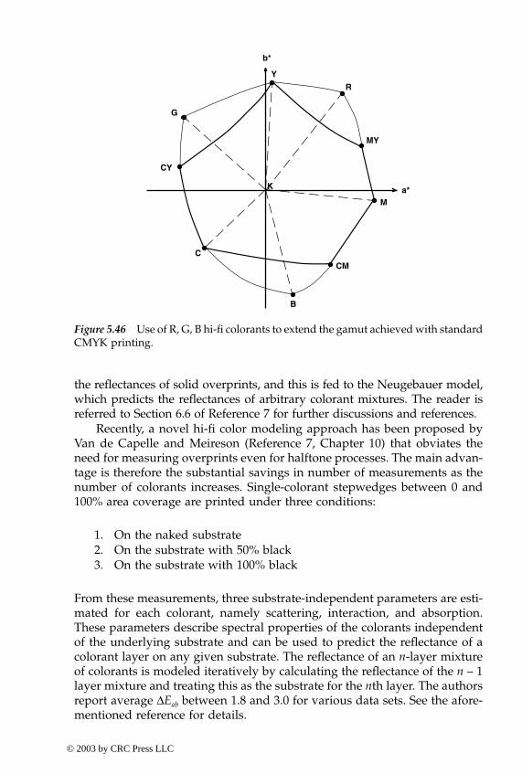
Chapter five: Device characterization 369
the reflectances of solid overprints, and this is fed to the Neugebauer model,which predicts the reflectances of arbitrary colorant mixtures. The reader isreferred to Section 6.6 of Reference 7 for further discussions and references.
Recently, a novel hi-fi color modeling approach has been proposed byVan de Capelle and Meireson (Reference 7, Chapter 10) that obviates theneed for measuring overprints even for halftone processes. The main advan-tage is therefore the substantial savings in number of measurements as thenumber of colorants increases. Single-colorant stepwedges between 0 and100% area coverage are printed under three conditions:
1. On the naked substrate2. On the substrate with 50% black 3. On the substrate with 100% black
From these measurements, three substrate-independent parameters are esti-mated for each colorant, namely scattering, interaction, and absorption.These parameters describe spectral properties of the colorants independentof the underlying substrate and can be used to predict the reflectance of acolorant layer on any given substrate. The reflectance of an n-layer mixtureof colorants is modeled iteratively by calculating the reflectance of the n – 1layer mixture and treating this as the substrate for the nth layer. The authorsreport average ∆Eab between 1.8 and 3.0 for various data sets. See the afore-mentioned reference for details.
b*
a*
R
Y
MY
M
CM
B
C
CY
G
K
Figure 5.46 Use of R, G, B hi-fi colorants to extend the gamut achieved with standardCMYK printing.
-ColorBook Page 369 Wednesday, November 13, 2002 10:55 AM
© 2003 by CRC Press LLC
370 Digital Color Imaging Handbook
5.10.7.2 Inverse characterizationAs with CMYK printing, hi-fi color introduces redundancy into the colorreproduction process in that many colorant combinations can result in thesame perceived (CIE) color. The inversion process must select a uniquecolorant combination for each input CIE color. Additional considerationsinclude minimization of colorant area coverage, minimization of moiré inthe case of rotated halftone screening, and a smooth characterization functionfrom CIE to device signals.
A common strategy is to partition the color gamut into subgamutsformed from combinations of three or four colorants. Referring to Figure5.46, one approach is to partition the gamut into six subgamuts formed fromthe following colorant combinations: CGK, GYK, YRK, RMK, MBK, andBCK. Here, R, G, and B represent hi-fi colorants chosen in the red, green,and blue hues.80,81 (Often, orange is used instead of red; the idea still holds.)Because C + Y combinations are spectrally redundant with G, the former aredisallowed, and only C + G and G + Y combinations are entertained. Thisrule guarantees uniqueness, and is applied likewise for the other combina-tions. Also, because only three screens angles are being used to render anygiven input color, moiré can be handled using the same rules applied forconventional printing. Another variant82 represents the gamut as overlap-ping subgamuts formed by GYRK, YRMK, RMBK, MBCK, BCGK, andCGYK. Several criteria, including minimization of colorant area coverageand smoothness of transitions across subgamuts, are used to select uniquecolorant combinations for a given input color. A third variant83 employs anapproach directly akin to UCR and GCR for CMYK printing. The gamut ispartitioned into the subgamuts formed by YRMK, MBCK, and CGYK. In theYRMK subgamut, the M and Y signals are fed to an R addition function andMY subtraction function. Analogous operations are applied in the othersubgamuts. The functions are chosen to produce a unique colorant combi-nation for each input color while maximizing the volume of each subgamut.As with conventional UCR/GCR, the latter can be aided by applying anonlinearity to the input signal and inverting this after the addition andsubtraction operations have been performed. Note that, with all theseapproaches, hi-fi colorants are used to render colors that can also be achievedwith standard CMYK colorants. In a fourth variant, only CMYK colorantsare used to achieve colors within the standard CMYK gamut, and hi-ficolorants are introduced only in those regions of color space that cannot bereproduced with CMYK mixtures. This approach offers better compatibilitywith standard CMYK devices. Details of these techniques are deferred to thestated references.
5.10.8 Projection transparency printing
Overhead transparency projection continues to be a common medium forcommunication of color information. Characterization for this application iscomplicated by several factors. First, the final viewing conditions and
-ColorBook Page 370 Wednesday, November 13, 2002 10:55 AM
© 2003 by CRC Press LLC
Chapter five: Device characterization 371
projector characteristics are difficult to predict a priori and may be verydifferent from those used for characterization. Second, it is difficult to achievestrict spatial uniformity, especially when the image is projected into a largescreen. Fortunately, color accuracy requirements for projected transparencyare usually not so stringent as to require careful characterization. But, ifaccuracy is important, care must be taken to control the aforementionedconditions as well as possible.
The characterization procedure is conceptually the same as for conven-tional printers. A test target is printed on a transparency and projected underrepresentative viewing conditions. The main factor that affects the latter isambient lighting. The projected image is measured with a spectroradiometer.To minimize light scattering, the transparency can be masked to present onlyone patch at a time to the spectroradiometer. The measured CIELAB valuesand original printer coordinates are then used to build the characterizationtransform. For all the reasons stated above, a simple transparency modelsuch as the Beer–Bouguer formula in Equation 5.64 may not suffice to predictthe characterization; rather, empirical approaches and three-dimensionalLUTs may be necessary to capture the various complex effects. The techniquesdescribed in Section 5.4 and Section 5.10.3 can be used for this purpose. Forfurther reading, see Chapter 10 of Kang48 and the work by Cui et al.84
5.11 Characterization for multispectral imaging The discussion in this chapter is primarily based on colorimetric reproduc-tion wherein the device-independent representation of Figure 5.1 comprisesthree color channels. An emerging area of research that is gaining increasingattention is multispectral imaging, whereby the goal is to capture, store, andreproduce narrowband spectral information rather than three-dimensionalcolorimetric data. A primary motivation for preserving spectral informationis that it mitigates the metamerism problems encountered in conventionalcolorimetric reproduction. A related advantage is that colorimetric charac-terizations can be computed dynamically for different viewing illuminantsfrom one set of spectral data. A schematic of a spectral imaging system isshown in Figure 5.47. The input device records color in N channels, whereN is greater than three. This is usually accomplished by using N narrowbandfilters in the image acquisition device. Spectral information is reconstructedfrom the data via spectral characterization of the input device.
A major concern in spectral imaging is the substantial increase in theamount of data to be handled (i.e., from 3 to 30 or more channels). Thisnecessitates an efficient encoding scheme for spectral data. Most encodingtechniques are based on the well-known fact that spectra found in natureare generally smooth and can be well approximated by a small number (i.e.,between five and eight) of basis functions.85 The latter can be derived viaprincipal-component analysis (PCA) described in an Chapter 1. PCA yieldsa compact encoding for spectral data and can serve as the device-indepen-dent color space in a multispectral imaging framework. An important con-
-ColorBook Page 371 Wednesday, November 13, 2002 10:55 AM
© 2003 by CRC Press LLC
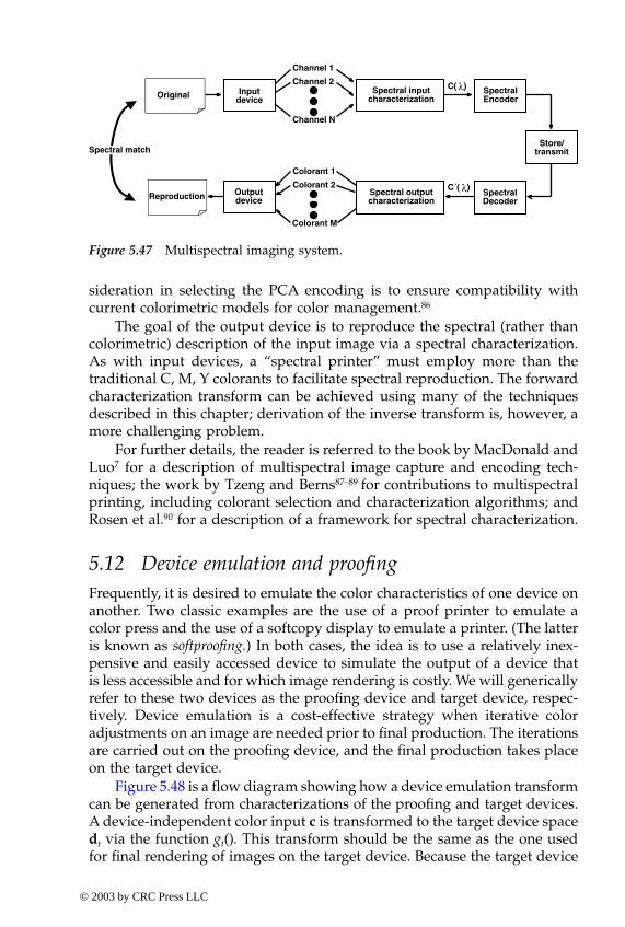
372 Digital Color Imaging Handbook
sideration in selecting the PCA encoding is to ensure compatibility withcurrent colorimetric models for color management.86
The goal of the output device is to reproduce the spectral (rather thancolorimetric) description of the input image via a spectral characterization.As with input devices, a “spectral printer” must employ more than thetraditional C, M, Y colorants to facilitate spectral reproduction. The forwardcharacterization transform can be achieved using many of the techniquesdescribed in this chapter; derivation of the inverse transform is, however, amore challenging problem.
For further details, the reader is referred to the book by MacDonald andLuo7 for a description of multispectral image capture and encoding tech-niques; the work by Tzeng and Berns87–89 for contributions to multispectralprinting, including colorant selection and characterization algorithms; andRosen et al.90 for a description of a framework for spectral characterization.
5.12 Device emulation and proofingFrequently, it is desired to emulate the color characteristics of one device onanother. Two classic examples are the use of a proof printer to emulate acolor press and the use of a softcopy display to emulate a printer. (The latteris known as softproofing.) In both cases, the idea is to use a relatively inex-pensive and easily accessed device to simulate the output of a device thatis less accessible and for which image rendering is costly. We will genericallyrefer to these two devices as the proofing device and target device, respec-tively. Device emulation is a cost-effective strategy when iterative coloradjustments on an image are needed prior to final production. The iterationsare carried out on the proofing device, and the final production takes placeon the target device.
Figure 5.48 is a flow diagram showing how a device emulation transformcan be generated from characterizations of the proofing and target devices.A device-independent color input c is transformed to the target device spacedt via the function gt(). This transform should be the same as the one usedfor final rendering of images on the target device. Because the target device
Original
Reproduction
Channel 1
Channel 2
Channel N
Spectral match
Inputdevice
SpectralEncoder
C( λ)Spectral inputcharacterization
Outputdevice
Colorant 1
Colorant 2
Colorant M
Spectral outputcharacterization
C´( λ)SpectralDecoder
Store/transmit
Figure 5.47 Multispectral imaging system.
-ColorBook Page 372 Wednesday, November 13, 2002 10:55 AM
© 2003 by CRC Press LLC
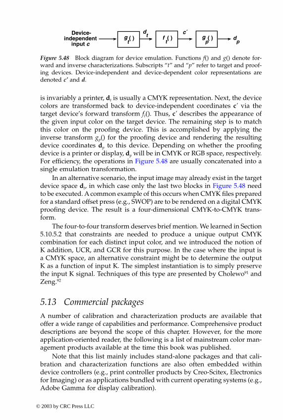
Chapter five: Device characterization 373
is invariably a printer, dt is usually a CMYK representation. Next, the devicecolors are transformed back to device-independent coordinates c’ via thetarget device’s forward transform ft(). Thus, c’ describes the appearance ofthe given input color on the target device. The remaining step is to matchthis color on the proofing device. This is accomplished by applying theinverse transform gp() for the proofing device and rendering the resultingdevice coordinates dp to this device. Depending on whether the proofingdevice is a printer or display, dp will be in CMYK or RGB space, respectively.For efficiency, the operations in Figure 5.48 are usually concatenated into asingle emulation transformation.
In an alternative scenario, the input image may already exist in the targetdevice space dt, in which case only the last two blocks in Figure 5.48 needto be executed. A common example of this occurs when CMYK files preparedfor a standard offset press (e.g., SWOP) are to be rendered on a digital CMYKproofing device. The result is a four-dimensional CMYK-to-CMYK trans-form.
The four-to-four transform deserves brief mention. We learned in Section5.10.5.2 that constraints are needed to produce a unique output CMYKcombination for each distinct input color, and we introduced the notion ofK addition, UCR, and GCR for this purpose. In the case where the input isa CMYK space, an alternative constraint might be to determine the outputK as a function of input K. The simplest instantiation is to simply preservethe input K signal. Techniques of this type are presented by Cholewo91 andZeng.92
5.13 Commercial packagesA number of calibration and characterization products are available thatoffer a wide range of capabilities and performance. Comprehensive productdescriptions are beyond the scope of this chapter. However, for the moreapplication-oriented reader, the following is a list of mainstream color man-agement products available at the time this book was published.
Note that this list mainly includes stand-alone packages and that cali-bration and characterization functions are also often embedded withindevice controllers (e.g., print controller products by Creo-Scitex, Electronicsfor Imaging) or as applications bundled with current operating systems (e.g.,Adobe Gamma for display calibration).
gt( )
c´Device-independent
input cf
t( ) g
p( )
dt d
p
Figure 5.48 Block diagram for device emulation. Functions f() and g() denote for-ward and inverse characterizations. Subscripts “t” and “p” refer to target and proof-ing devices. Device-independent and device-dependent color representations aredenoted c’ and d.
-ColorBook Page 373 Wednesday, November 13, 2002 10:55 AM
© 2003 by CRC Press LLC
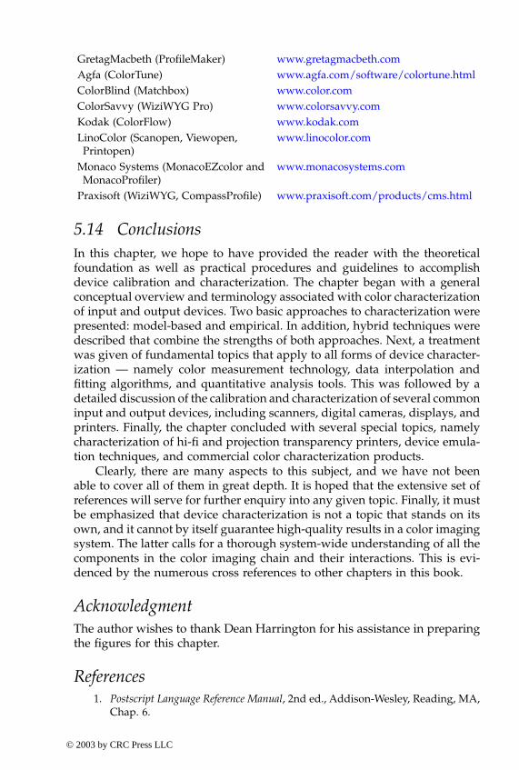
374 Digital Color Imaging Handbook
5.14 ConclusionsIn this chapter, we hope to have provided the reader with the theoreticalfoundation as well as practical procedures and guidelines to accomplishdevice calibration and characterization. The chapter began with a generalconceptual overview and terminology associated with color characterizationof input and output devices. Two basic approaches to characterization werepresented: model-based and empirical. In addition, hybrid techniques weredescribed that combine the strengths of both approaches. Next, a treatmentwas given of fundamental topics that apply to all forms of device character-ization — namely color measurement technology, data interpolation andfitting algorithms, and quantitative analysis tools. This was followed by adetailed discussion of the calibration and characterization of several commoninput and output devices, including scanners, digital cameras, displays, andprinters. Finally, the chapter concluded with several special topics, namelycharacterization of hi-fi and projection transparency printers, device emula-tion techniques, and commercial color characterization products.
Clearly, there are many aspects to this subject, and we have not beenable to cover all of them in great depth. It is hoped that the extensive set ofreferences will serve for further enquiry into any given topic. Finally, it mustbe emphasized that device characterization is not a topic that stands on itsown, and it cannot by itself guarantee high-quality results in a color imagingsystem. The latter calls for a thorough system-wide understanding of all thecomponents in the color imaging chain and their interactions. This is evi-denced by the numerous cross references to other chapters in this book.
AcknowledgmentThe author wishes to thank Dean Harrington for his assistance in preparingthe figures for this chapter.
References1. Postscript Language Reference Manual, 2nd ed., Addison-Wesley, Reading, MA,
Chap. 6.
GretagMacbeth (ProfileMaker) www.gretagmacbeth.comAgfa (ColorTune) www.agfa.com/software/colortune.htmlColorBlind (Matchbox) www.color.comColorSavvy (WiziWYG Pro) www.colorsavvy.comKodak (ColorFlow) www.kodak.comLinoColor (Scanopen, Viewopen, Printopen)
www.linocolor.com
Monaco Systems (MonacoEZcolor and MonacoProfiler)
www.monacosystems.com
Praxisoft (WiziWYG, CompassProfile) www.praxisoft.com/products/cms.html
-ColorBook Page 374 Wednesday, November 13, 2002 10:55 AM
© 2003 by CRC Press LLC
Chapter five: Device characterization 375
2. Trussell, H. J., DSP solutions run the gamut for color systems, IEEE SignalProcessing, 10, 8–23, 1993.
3. Luther, R., Aus Dem Gebiet der Farbreizmetrik, Z. Tech. Phys., 8, 540–558, 1927.4. Ives, H. E., The transformation of color-mixture equations from one system
to another, J. Franklin Inst., 16, 673–701, 1915.5. Sharma, G. and Trussell, H. J., Color scanner performance trade-offs, in Proc.
SPIE, Color Imaging: Device-Independent Color, Color Hardcopy, and Graphic Arts,J. Bares, Ed., Vol. 2658, 1996, 270–278.
6. Sharma, G. Trussell, G, H. J, and Vrhel, M. J., Optimal non-negative colorscanning filters, IEEE Trans. Image Proc., 7(1), 129–133, 1998.
7. MacDonald, L. W. and Luo, M. R., Eds., Colour Imaging — Vision and Technol-ogy, Wiley, Chichester, U.K., 1999.
8. Alessi, P. J. and Cottone, P. L., Color reproduction scheme for Kodak OrganicLight Emitting Diode (OLED) technology, AIC Color 01, Rochester, NY, June24–29, 2001.
9. Rich, D., Critical parameters in the measurement of the color of nonimpactprinting, J. Electronic Imaging, 2(3), 1993, 23–236, 1993.
10. Zwinkels, J. C., Colour-measuring instruments and their calibration, Displays,16(4), 163–171, 1996.
11. Rolleston, R., Using Shepard’s interpolation to build color transformationtables, in Proc. IS&T/SID’s 2nd Color Imaging Conference, November 1994,74–77.
12. R. Balasubramanian, Refinement of printer transformations using weightedregression, in Proc. SPIE, Color Imaging: Device-Independent Color, Color Hard-copy, and Graphic Arts, J. Bares, Ed., Vol. 2658, 1996, 334–340.
13. Hung, P-C., Colorimetric calibration in electronic imaging devices using alook-up table model and interpolations, J. Electronic Imaging, 2(1), 53–61, 1993.
14. Chang, J. Z., Allebach, J. P., and Bouman, C. A., Sequential linear interpolationof multidimensional functions, IEEE Trans. on Image Processing, Vol. IP-6,September 1997, 1231–1245.
15. T. Masters, Practical Neural Network Recipes in C++, Academic Press, San Diego,CA, 1993.
16. Farin, G., Curves and Surfaces for Computer Aided Geometric Design — A PracticalGuide, Academic Press, San Diego, CA, 1988.
17. Press, H., Flannery, B. P., and Vetterling, W. T., Numerical Recipes in C, Cam-bridge University Press, Cambridge, U.K., 1988.
18. Luo, M. R., Cui, G. and Rigg, B., The development of the CIEDE2000 colour-difference formula, Color Res. Appl., 25, 340–350, 2001.
19. Engeldrum, P. G., Psychometric Scaling, Imcotek Press, Winchester, MA, 2000.20. Sharma, G. and Trussell, H. J., Figures of merit for color scanners, IEEE Trans.
Image Proc., 6(7), 990–1001, 1997.21. Quan, S. and Ohta, N., Optimization of camera spectral sensitivities, in Proc.
IS&T/SID’s 8th Color Imaging Conference, November 2000, 273–278.22. Knox, K. T., Integrating cavity effect in scanners, in Proc. IS&T/OSA Optics &
Imaging in the Information Age, Rochester NY, 1996, 156–158.23. Kang, H. R., Color scanner calibration, J. Imaging Sci. Technol., 36(2), 162–170,
1992.24. Sharma, G. and Trussell, H. J., Set theoretic estimation in color scanner char-
acterization, J. Electronic Imaging, 5(4), 479–489, 1996.25. Wandell, B. A., Foundations of Vision, Sinauer Associates, Sunderland, MA, 1995.
-ColorBook Page 375 Wednesday, November 13, 2002 10:55 AM
© 2003 by CRC Press LLC
376 Digital Color Imaging Handbook
26. Finlayson, G. D., Hordley, S., and Hubel, P. M., Recovering device sensitivitieswith quadratic programming, in Proc. IS&T/SID’s 6th Color Imaging Conference,November 1998, 90–95.
27. Hubel, P. M., Sherman, D., and Farrell, J. E., A comparison of methods ofsensor spectral sensitivity estimation, in Proc. IS&T/SID’s 2nd Color ImagingConference, November 1994, 45–48.
28. Finlayson, G. D. and Drew, M. S., The maximum ignorance assumption withpositivity, in Proc. IS&T/SID’s 4th Color Imaging Conference, November 1996,202–205.
29. Berns, R. and Shyu, M. J., Colorimetric characterization of a desktop drumscanner using a spectral model, J. Electronic Imaging, 4(4), 360–372, 1995.
30. Sharma, G., Target-less scanner color calibration, J. Imaging Sci. Technol., 44(4),301–307, 2000.
31. Kang, H. R. and Anderson, P. G., Neural network applications to the colorscanner and printer calibrations, J. Electronic Imaging, 1(2), 125–135, 1992.
32. ISO 17321 (WD4), Graphic Technology and Photography — Colour Characterisationof Digital Still Cameras (DSCs) Using Colour Targets and Spectral Illumination.
33. ISO 14525 (FDIS), Photography — Electronic Still Picture Cameras — Methods ofMeasuring Opto-Electronic Conversion Functions (OECFs).
34. Finlayson, G. D. and Drew, M. S., White point preserving color correction, inProc. IS&T/SID’s 5th Color Imaging Conference, November 1997, 258–61.
35. Hubel, P. M. et al., Matrix calculations for digital photography, in Proc.IS&T/SID’s 5th Color Imaging Conference, November 1997, 105–111.
36. Hong, G., Han, B., and Luo, M. R., Colorimetric characterisation for low-enddigital camera, in Proc. 4th International Conference on Imaging Science andHardcopy, 2001, 21–24.
37. Hong, G., Luo, M. R., and Rhodes, P. A., A study of digital camera colorimetriccharacterisation based on polynomial modelling, Color Res. Appl., 26(1), 76–84,2001.
38. Finlayson, G. D., Drew, M. S., and Funt, B. V., Spectral sharpening: Sensortransformations for improved colour constancy, J. Opt. Soc. Am., 5, 1553–1563,1994.
39. Berns, R., S. Motta, R. J., and Gorzynski, M. E., CRT Colorimetry, Part 1:Theory and practice, Color Res. Appli., 18(5), 299–314, 1993.
40. Edgar, A. D. and Kasson, J. M., Display Calibration, U.S. Patent No. 5,298,993,issued March 29, 1994.
41. Engeldrum, P. and Hilliard, W., Interactive Method and System for ColorCharacterization and Calibration of Display Device, U.S. Patent No. 5,638,117,issued June 10, 1997.
42. Ohara, K. et al., Apparatus for Determining a Black Point on a Display Unitand Method of Performing the Same, U.S. Patent No. 6,084,564, issued July4, 2000.
43. Balasubramanian, R., Braun, K., Buckley, R., and Rolleston, R., Color docu-ments in the Internet era, The Industrial Physicist, 16–20, 2001.
44. Gentile, R. S. and Danciu, I. M., Method to estimate the white point on adisplay device, U.S. Patent No. 6,023,264, issued February 8, 2000.
45. Marcu, G. et al., Color characterization issues for TFTLCD displays, in Proc.SPIE, Color Imaging: Device-Independent Color, Color Hardcopy, and ApplicationsVII, Eschbach, R. and Marcu, G., Eds., Vol. 4663, 2002, 187–198.
-ColorBook Page 376 Wednesday, November 13, 2002 10:55 AM
© 2003 by CRC Press LLC
Chapter five: Device characterization 377
46. Sharma, G., Comparative evaluation of color characterization and gamut ofLCDs versus CRTs, in Proc. SPIE, Color Imaging: Device-Independent Color, ColorHardcopy, and Applications VII, Eschbach, R. and Marcu, G., Eds., Vol. 4663,2002, 177–186.
47. Kwak, Y. and MacDonald, L. Accurate prediction of colours on liquid crystaldisplays, in Proc. IS&T/SID’s 9th Color Imaging Conference, November 2001,355–359.
48. H. R. Kang, Color Technology for Electronic Imaging Devices, SPIE, Bellingham,WA, 1997.
49. Bala, R., What is the chrominance of gray? Proc. IS&T and SID’s 9th ColorImaging Conference, November 2001, 102–107.
50. Yule, J. A. C., Principles of Color Reproduction: Applied to Photomechanical Repro-duction, Color Photography, and the Ink, Paper, and Other Related Industries, JohnWiley & Sons, New York, 1967.
51. Allen, E., Optical Radiation Measurements, Vol. 2., Color Formulation and Shading,Academic Press, San Diego, CA, 1980, Chap. 7.
52. Berns, R. S., Spectral modeling of a dye diffusion thermal transfer printer, J.Electronic Imaging, 2(4), 359–370, 1993.
53. Parton, K. H. and Berns, R. S., Color modeling ink-jet ink on paper usingKubelka–Munk theory, in Proc. 7th Int. Congress on Advances in Non-ImpactPrinting Technologies, 1992, 271–280.
54. Kang, H. R., Kubelka–Munk modeling of ink jet ink mixing, J. Imaging Technol.,17, 76–83, 1991.
55. Saunderson, J. L., Calculation of the color of pigmented plastics, J. OpticalSoc. Am., 32, 727–736, 1942.
56. Neugebauer, H. E. J., Die Theoretischen Grandlagen des Mehrfarben-edruck-es, Zeitschrift Wissenschaften Photography, 73–89, 1937.
57. Rolleston, R. and Balasubramanian, R., Accuracy of various types of Neuge-bauer models, in Proc. IS&T and SID‘s 1st Color Imaging Conference: Transformsand Transportability of Color, November 1993, 32–37.
58. Viggiano, J. A. S., Modeling the color of multi-colored halftones, in Proc.TAGA, 44–62, 1990.
59. Balasubramanian, R., Optimization of the spectral Neugebauer model forprinter characterization, J. Electronic Imaging, 8(2), 156–166, 1999.
60. Yule, J. A. C. and Nielsen, W. J., The penetration of light into paper and itseffect on halftone reproduction, in Proc. TAGA, 65–76, 1951.
61. Maltz, M., Light scattering in xerographic images, J. Appl. Photogr. Eng., 9(3),83–89, 1983.
62. Gustavson, S. and Kruse, B., 3D modelling of light diffusion in paper, in Proc.TAGA, 2, 848–855, 1995.
63. Heuberger, K. J., Jing, Z. M., and Persiev, S., Color transformations and lookuptables, in Proc. TAGA/ISCC, 2, 863–881, 1992.
64. Arney, J. S., Engeldrum, P. G., and Zeng, H., An expanded Murray–Daviesmodel of tone reproduction in halftone imaging, J. Imaging Sci. Technol., 39(6),502–508, 1995.
65. Lee, B. et al., Estimation of the Neugebauer model of a halftone printer andits application, in Proc. IS&T/OSA Annu. Conf., Optics & Imaging in the Infor-mation Age, 1997, 610–613.
-ColorBook Page 377 Wednesday, November 13, 2002 10:55 AM
© 2003 by CRC Press LLC
378 Digital Color Imaging Handbook
66. Iino, K. and Berns, R. S., A spectral based model of color printing that com-pensates for optical interactions of multiple inks, AIC Color 97, in Proc. 8thCongress International Colour Association, 1997, 610–613.
67. Hau, C. and Huang, K., Advanced cellular YNSN printer model, in Proc.IS&T/SID’s 5th Color Imaging Conf., November 1997, 231–234.
68. Iino, K. and Berns, R. S., Building color management modules using linearoptimization, I. Desktop color system, J. Imaging Sci. Tech. 42(1), 79–94, 1998.
69. Iino, K. and Berns, R. S., Building color management modules using linearoptimization, II. Prepress system for offset printing, J. Imaging Sci. Technol.,42(2), 99–114, 1998.
70. Agar, A. U. and Allebach, J. P., An iterative cellular YNSN method for colorprinter characterization, in Proc. IS&T/SID’s 6th Color Imaging Conference, No-vember 1998, 197–200.
71. Xia, M. et al., End-to-end color printer calibration by total least squaresregression, IEEE Trans. Image Proc., 8(5), 700–716, 1999.
72. Balasubramanian, R., Reducing the cost of lookup table based color transfor-mations, J. Imaging Sci. Technol., 44(4), 321–327, 2000.
73. Herzog, P., A new approach to printer calibration based on nested gamutshells, in Proc. IS&T/SID’s 5th Color Imaging Conference, November 1997,245–249.
74. Pobboravsky, I. and Pearson, M., Computation of dot areas required to matcha colorimetrically specified color using the modified Neugebauer equations,in Proc. TAGA, 65–77, 1972.
75. Mahy, M. and Delabastita, P., Inversion of the Neugebauer equations, ColorRes. Appl., 21(6), 404–411, 1996.
76. Holub, R., Pearson, C., and Kearsley, W., The black printer, J. Imaging Technol.,15(4), 149–158, 1989.
77. Mahy, M., Color Separation Method and Apparatus for Same, U.S. Patent No.5,878,195, issued March 2, 1999.
78. Balasubramanian, R. and Eschbach, R., Reducing multi-separation color moi-re via a variable undercolor removal and gray-component replacement strat-egy, J. Imaging Sci. Technol., 45(2), 152–160, 2001.
79. Cholewo, T. J., Printer model inversion by constrained optimization, in Proc.SPIE, Color Imaging: Device-Independent Color, Color Hardcopy, and Graphic ArtsV, R. Eschbach and G. Marcu, Eds., Vol. 3963, San Jose, CA, 2000, 349–357.
80. Kueppers, H., Printing Process where Each Incremental Area is Divided intoa Chromatic Area and an Achromatic Area and Wherein the Achromatic AreasAre Printed in Black and White and the Chromatic Areas are Printed in ColorSub-sections, U.S. Patent No. 4,812,899, issued March 14, 1989.
81. Ostromoukhov V., Chromaticity gamut enhancement by heptatone multi-color printing, in Proc. SPIE, Device Independent Color Imaging and ImagingSystems Integration, Motta R. J. and Berberian, H. A., Eds., Vol. 1909, 1993,139–151.
82. Boll, H., A color to colorant transformation for a seven ink process, in Proc.SPIE, Device Independent Color Imaging, Walowit E., Ed., Vol. 2170, 1994,108–118.
83. Balasubramanian, R., System for Printing Color Images with Extra Colorantsin Addition to Primary Colorants, U.S. Patent No. 5,870,530, issued Feb. 9,1999.
-ColorBook Page 378 Wednesday, November 13, 2002 10:55 AM
© 2003 by CRC Press LLC
Chapter five: Device characterization 379
84. Cui, C. and Weed, S., Measurement problems for overhead projection trans-parency printing color calibration, in Proc. IS&T/SID’s 9th Color Imaging Con-ference, November 2001, 303–309.
85. Vrhel, M. J., Gershon, R., and Iwan, L. S., Measurement and analysis of objectreflectance spectra, Color Res. Appl., 19(1), 4–9, 1991.
86. Keusen, T., Multispectral color system with an encoding format compatiblewith the conventional tristimulus model, J. Imaging Sci. Technol., 40(6),510–515, 1996.
87. Tzeng, D. Y. and Berns, R. S., Spectral-based six-color separation minimizingmetamerism, in Proc. IS&T/SID’s 8th Color Imaging Conference, November 2000,342–347.
88. Tzeng, D. Y. and Berns, R. S., Spectral-based ink selection for multiple-inkprinting I. Colorants estimation of original objects, in Proc. IS&T/SID’s 6thColor Imaging Conference, November 1998, 106–111.
89. Tzeng, D. Y. and Berns, R. S., Spectral-based ink selection for multiple-inkprinting II. Optimal ink selection, in Proc. IS&T/SID’s 7th Color Imaging Con-ference, November 1999, 182–187.
90. Rosen, M. R. et al., Color management within a spectral image visualizationtool, in Proc. IS&T/SID’s 8th Color Imaging Conference, November 2000, 75–80.
91. Cholewo, T. J., Conversion between CMYK spaces preserving black separa-tion, in Proc. IS&T/SID’s 8th Color Imaging Conference, November 2000,257–261.
92. Zeng, H., CMYK transformation with black preservation in color manage-ment system, in Proc. SPIE, Color Imaging: Device-Independent Color, Color Hard-copy, and Applications VII, Eschbach, R. and Marcu, G., Eds., Vol. 4663, 2002,143–149.
93. Noble, B. and Daniel, J. W., Applied Linear Algebra, 2nd ed., Chapter 9, Prentice-Hall, Englewood Cliffs, NJ, 1977, 323–330.
-ColorBook Page 379 Wednesday, November 13, 2002 10:55 AM
© 2003 by CRC Press LLC
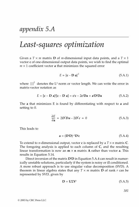
3810-8493-0900-X/03/$0.00+$1.50© 2003 by CRC Press LLC
appendix 5.A
Least-squares optimization
Given a T × m matrix D of m-dimensional input data points, and a T × 1vector c of one-dimensional output data points, we wish to find the optimalm × 1 coefficient vector a that minimizes the squared error
(5.A.1)
where denotes the L2 norm or vector length. We can write the error inmatrix-vector notation as
E = [c – D a]t[c – D a] = ctc – 2ctDa + atDtDa (5.A.2)
The a that minimizes E is found by differentiating with respect to a andsetting to 0.
(5.A.3)
This leads to
a = (DtD)–1Dtc (5.A.4)
To extend to n-dimensional output, vector c is replaced by a T × n matrix C.The foregoing analysis is applied to each column of C, and the resultinglinear transformation is now an m × n matrix A rather than vector a. Thisresults in Equation 5.14.
Direct inversion of the matrix DtD in Equation 5.A.4 can result in numer-ically unstable solutions, particularly if the system is noisy or ill conditioned.A more robust approach is to use singular value decomposition (SVD). Atheorem in linear algebra states that any T × m matrix D of rank r can berepresented by SVD, given by
D = UΣVt (5.A.5)
E c D a–= 2
2
∂E∂a------ 2DtDa 2Dtc– 0= =
-ColorBook Page 381 Wednesday, November 13, 2002 10:55 AM
© 2003 by CRC Press LLC
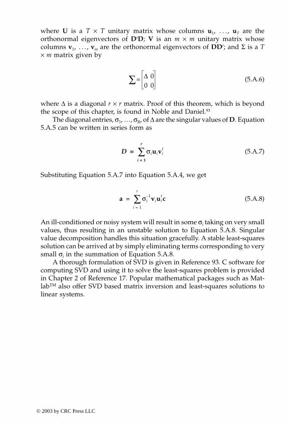
382 Digital Color Imaging Handbook
where U is a T × T unitary matrix whose columns u1, . . . , uT are theorthonormal eigenvectors of DtD; V is an m × m unitary matrix whosecolumns v1, . . . , vm are the orthonormal eigenvectors of DDt; and Σ is a T× m matrix given by
(5.A.6)
where ∆ is a diagonal r × r matrix. Proof of this theorem, which is beyondthe scope of this chapter, is found in Noble and Daniel.93
The diagonal entries, σ1, …, σR, of ∆ are the singular values of D. Equation5.A.5 can be written in series form as
(5.A.7)
Substituting Equation 5.A.7 into Equation 5.A.4, we get
(5.A.8)
An ill-conditioned or noisy system will result in some σi taking on very smallvalues, thus resulting in an unstable solution to Equation 5.A.8. Singularvalue decomposition handles this situation gracefully. A stable least-squaressolution can be arrived at by simply eliminating terms corresponding to verysmall σi in the summation of Equation 5.A.8.
A thorough formulation of SVD is given in Reference 93. C software forcomputing SVD and using it to solve the least-squares problem is providedin Chapter 2 of Reference 17. Popular mathematical packages such as Mat-labTM also offer SVD based matrix inversion and least-squares solutions tolinear systems.
=∑ ∆ 00 0
D σiuivit
i 1=
r
∑=
a σi1– viui
tci 1=
r
∑=
-ColorBook Page 382 Wednesday, November 13, 2002 10:55 AM
© 2003 by CRC Press LLC
383
0-8493-0900-X/03/$0.00+$1.50© 2003 by CRC Press LLC
appendix 5.B
Derivation of 3
¥
3 matrix from display RGB to XYZ given white point and chromaticities of the primaries
Given chromaticity coordinates of the three primaries, [x
R
, y
R
], [x
G
, y
G
], [x
B
,y
B
], and the tristimulus values of the white point, [X
w
, Y
w
, Z
w
], the goal is toderive the 3
¥
3 matrix
A
CRT
that maps display RGB to XYZ as in Equation 5.55.Assign an arbitrary value
Y
R
=
Y
G
=
Y
B
= 1 for the luminance of the threeprimaries. This provides three-dimensional xyY descriptors for the prima-ries.
Convert the xyY coordinates of each primary to XYZ space as follows:
(5.B.1)
Analogous expressions apply for the green and blue primaries. This definesa matrix
A
’ given by
(5.B.2)
We now have to scale the column vectors of
A
’ so that an input of RGB =[1, 1, 1] results in the desired white point [X
w
, Y
w
, Z
w
]. This is done by thefollowing operation:
XR, xR
yR-----= , YR
, 1= , ZR, 1 xR yR��
yR--------------------------Ë ¯
Ê � zR
yR-----= =
A,XR
, XG, XB
,
YR, YG
, YB,
ZR, ZG
, ZB,
xR yR§ xG yG§ xB yB§1 1 1
zR yR§ zG yG§ zB yB§
= =
05 Page 383 Monday, November 18, 2002 8:26 AM
© 2003 by CRC Press LLC

384 Digital Color Imaging Handbook
(5.B.3)
where W is the white vector.
ACRT A, * diag A, 1– * W( )=
-ColorBook Page 384 Wednesday, November 13, 2002 10:55 AM
© 2003 by CRC Press LLC