Embed Size (px)
Citation preview
Characterisation and Optimisation
of the Herschel-SPIRE Imaging
Photometer Through Simulations
by
Bruce Sibthorpe
A thesis submitted to
Cardiff University
for the degree of
Doctor of Philosophy
2007


DECLARATION
This work has not previously been accepted in substance for any degree andis not concurrently submitted in candidature for any degree.
Signed ........................................... Date ..............................................
STATEMENT 1
This thesis is being submitted in partial fulfillment of the requirements forthe degree of PhD
Signed ........................................... Date ..............................................
STATEMENT 2
This thesis is the result of my own independent work/investigation, exceptwhere otherwise stated. Other sources are acknowledged by explicit refer-ences.
Signed ........................................... Date ..............................................
STATEMENT 3
I hereby give consent for my thesis, if accepted, to be available for photo-copying and for inter-library loans after expiry of a bar on access approvedby the Graduate Development Committee.
Signed ........................................... Date ..............................................

Acknowledgments
Foremost I would like to thank my supervisor Matt Griffin for his supportthroughout this project, and particularly for his help in drafting this the-sis. I also thank Phil Mauskopf, Tim Waskett, and Pete Hargrave for theirsignificant contributions to this work, and for their advice.
Furthermore I would like to thank Emma for the love and encouragementshe has given me over the course of this work.
I must also acknowledge the entire BLAST consortium for their help andfriendship. I would specifically like to recognise Edward Chapin and Guil-laume Patanchon for their contributions to the BLAST work presented inthis thesis.
In addition to those directly involved with my work I would also like to thankDerek Ward-Thompson, Dave Nutter, Jason Kirk, Haley Gomez and LloydWatkin, all of whom have provided useful guidance throughout this project.
I’d like to thank my housemates Robbie Auld, Gustav Teleberg and MikeZemcov, as well as all of my friends for their help, support, and friendship.They have made my time on this project a fun and happy one.
Finally I thank my parents for their continued support and encouragementin this and future work.

Abstract
The Spectral and Photometric Imaging Receiver (SPIRE) is one of the threeinstruments on-board the European Space Agency’s Herschel Space Obser-vatory, due for launch in 2008. SPIRE is a dual instrument comprising aphotometer, and imaging Fourier transform spectrometer.
This thesis deals with the design and operation of a software simulator forthe SPIRE photometer. The simulator architecture and modelling methodsare described, and the fidelity of its output verified.
This simulation software is then used to optimise and characterise data fromthe SPIRE photometer. The optimum observing parameters are derived, inorder to maximise observing efficiency, and data quality. The impact of un-correlated 1/f noise on the extraction of sources of arbitrary scale is assessed,and quantified. This work is also extended to include the impact of uncorre-lated 1/f noise on observations of sources in a confused environment. Theseresults provide important information regarding the quality of SPIRE pho-tometer data for the planning of large survey observations. The simulator isalso an active tool within the SPIRE Instrument Control Centre team, andits use in the selection of the SPIRE map making algorithm is described.
This thesis also contains an analysis of observations of the Cassiopeia Asupernova remnant made with the Balloon-borne Large Aperture submil-limetre Telescope (BLAST), an instrument based on the SPIRE photometerdesign. This analysis assesses the hypothesis that supernovae might be asignificant dust formation mechanism in the universe, as proposed in recentliterature. Results from this study suggest that this hypothesis may be cor-rect, but that evidence from previous observations might in fact be upperlimits to the total mass of dust, rather than an absolute measurement.

Contents
1 Introduction 1
1.1 FIR and Submillimetre Astronomy . . . . . . . . . . . . . . . . 1
1.1.1 Observing in the FIR and Submillimetre . . . . . . . . 6
1.2 Herschel . . . . . . . . . . . . . . . . . . . . . . . . . . . . . . . 9
1.2.1 Herschel Science . . . . . . . . . . . . . . . . . . . . . . 11
1.2.2 The Herschel Spacecraft . . . . . . . . . . . . . . . . . . 12
1.2.3 Instruments . . . . . . . . . . . . . . . . . . . . . . . . . 13
1.3 BLAST . . . . . . . . . . . . . . . . . . . . . . . . . . . . . . . . 16
1.4 Bolometers . . . . . . . . . . . . . . . . . . . . . . . . . . . . . . 18
1.5 Chapter Summary . . . . . . . . . . . . . . . . . . . . . . . . . . 23
1.6 Outline of this Thesis . . . . . . . . . . . . . . . . . . . . . . . . 24
2 Dust in the Interstellar Medium 27
2.1 The Interstellar Medium . . . . . . . . . . . . . . . . . . . . . . 27
2.1.1 The Dust Cycle . . . . . . . . . . . . . . . . . . . . . . . 28
2.2 The Origin of Dust in the ISM . . . . . . . . . . . . . . . . . . . 29
2.2.1 The Classical Theory of Dust Formation . . . . . . . . . 30
i
ii CONTENTS
2.2.2 The Dust Debt . . . . . . . . . . . . . . . . . . . . . . . . 32
2.2.3 An Alternative Source of Dust . . . . . . . . . . . . . . . 33
2.3 Star Formation . . . . . . . . . . . . . . . . . . . . . . . . . . . 34
2.3.1 Core Structure and Support . . . . . . . . . . . . . . . . 35
2.3.2 Core Collapse . . . . . . . . . . . . . . . . . . . . . . . . 35
2.3.3 Collapse Solutions . . . . . . . . . . . . . . . . . . . . . . 38
2.4 Observational Properties of Dust . . . . . . . . . . . . . . . . . 39
2.4.1 The Interaction of Dust with Radiation . . . . . . . . . 39
2.4.2 Estimating Dust Masses . . . . . . . . . . . . . . . . . . 40
2.4.3 Cirrus Confusion Noise . . . . . . . . . . . . . . . . . . . 42
2.5 Chapter Summary . . . . . . . . . . . . . . . . . . . . . . . . . . 44
3 SPIRE 47
3.1 Instrument Overview . . . . . . . . . . . . . . . . . . . . . . . . 48
3.1.1 Photometer . . . . . . . . . . . . . . . . . . . . . . . . . . 48
3.1.2 Spectrometer . . . . . . . . . . . . . . . . . . . . . . . . . 51
3.1.3 Optics . . . . . . . . . . . . . . . . . . . . . . . . . . . . . 53
3.1.4 Detector Assemblies . . . . . . . . . . . . . . . . . . . . 54
3.1.5 Thermal System . . . . . . . . . . . . . . . . . . . . . . . 54
3.1.6 Detector Read-Out . . . . . . . . . . . . . . . . . . . . . 56
3.2 Photometer Observatory Functions . . . . . . . . . . . . . . . . 56
3.2.1 Point Source Photometry . . . . . . . . . . . . . . . . . . 56
3.2.2 Field Jiggle Mapping . . . . . . . . . . . . . . . . . . . . 58
CONTENTS iii
3.2.3 Scan Mapping . . . . . . . . . . . . . . . . . . . . . . . . 59
3.3 SPIRE Scientific Programme . . . . . . . . . . . . . . . . . . . 59
3.4 Chapter Summary . . . . . . . . . . . . . . . . . . . . . . . . . . 65
4 The SPIRE Photometer Simulator 67
4.1 Introduction . . . . . . . . . . . . . . . . . . . . . . . . . . . . . 67
4.2 Simulator Development Plan . . . . . . . . . . . . . . . . . . . 70
4.3 Simulator Architecture . . . . . . . . . . . . . . . . . . . . . . . 70
4.3.1 Module Summary . . . . . . . . . . . . . . . . . . . . . . 71
4.4 SPS Operation . . . . . . . . . . . . . . . . . . . . . . . . . . . . 73
4.4.1 SPS Control . . . . . . . . . . . . . . . . . . . . . . . . . 73
4.4.2 Master Clock . . . . . . . . . . . . . . . . . . . . . . . . . 75
4.4.3 Parameters . . . . . . . . . . . . . . . . . . . . . . . . . . 75
4.4.4 Data Volume . . . . . . . . . . . . . . . . . . . . . . . . . 77
4.5 Coordinate Systems . . . . . . . . . . . . . . . . . . . . . . . . . 77
4.6 Module Operations . . . . . . . . . . . . . . . . . . . . . . . . . 78
4.6.1 Sky Simulator (Sky) . . . . . . . . . . . . . . . . . . . . 78
4.6.2 Observatory Function (Obsfun) . . . . . . . . . . . . . . 79
4.6.3 Optics Module (Optics) . . . . . . . . . . . . . . . . . . . 85
4.6.4 Thermal System (Thermal) . . . . . . . . . . . . . . . . 89
4.6.5 Beam Steering Mirror (BSM) . . . . . . . . . . . . . . . 91
4.6.6 Background Power Timeline Generator (Background) . 94
4.6.7 Astronomical Power Timeline Generator (Astropower) 95
iv CONTENTS
4.6.8 Detector Voltage Timeline Generator (Detectors) . . . . 96
4.6.9 Sampling System (Sampling) . . . . . . . . . . . . . . . 98
4.6.10 Simulator Operation . . . . . . . . . . . . . . . . . . . . 98
4.7 Chapter Summary . . . . . . . . . . . . . . . . . . . . . . . . . . 99
5 Data Reduction and Simulator Verification 101
5.1 Data Cleaning . . . . . . . . . . . . . . . . . . . . . . . . . . . . 102
5.2 Calibration . . . . . . . . . . . . . . . . . . . . . . . . . . . . . . 105
5.3 Map-Making . . . . . . . . . . . . . . . . . . . . . . . . . . . . . 105
5.4 Simulator Performance Verification . . . . . . . . . . . . . . . . 108
5.4.1 Point Source SNR Measurement . . . . . . . . . . . . . 108
5.4.2 Measuring the SNR of a Point Noise in a SimulatedOutput Map . . . . . . . . . . . . . . . . . . . . . . . . . 113
5.4.3 Simulator Verification . . . . . . . . . . . . . . . . . . . 116
5.5 The SPIRE Map-Making Algorithm . . . . . . . . . . . . . . . 118
5.6 Chapter Summary . . . . . . . . . . . . . . . . . . . . . . . . . . 120
6 Observing Mode Optimisation 129
6.1 Point Source Photometry . . . . . . . . . . . . . . . . . . . . . . 129
6.2 Field Mapping . . . . . . . . . . . . . . . . . . . . . . . . . . . . 131
6.3 Scan Mapping . . . . . . . . . . . . . . . . . . . . . . . . . . . . 134
6.4 Observing Mode Selection . . . . . . . . . . . . . . . . . . . . . 141
6.5 Chapter Summary . . . . . . . . . . . . . . . . . . . . . . . . . . 144
7 BLAST Observations of the Cassiopeia A 147
CONTENTS v
7.1 Introduction . . . . . . . . . . . . . . . . . . . . . . . . . . . . . 147
7.2 The Cassiopeia A Supernova Remnant . . . . . . . . . . . . . . 147
7.3 Dust Creation in SNe . . . . . . . . . . . . . . . . . . . . . . . . 149
7.4 Observations of Cas A with BLAST . . . . . . . . . . . . . . . . 153
7.4.1 The Data . . . . . . . . . . . . . . . . . . . . . . . . . . . 153
7.5 Data Reduction . . . . . . . . . . . . . . . . . . . . . . . . . . . 156
7.6 Data Analysis and Results . . . . . . . . . . . . . . . . . . . . . 156
7.6.1 Maps . . . . . . . . . . . . . . . . . . . . . . . . . . . . . 157
7.6.2 Photometry . . . . . . . . . . . . . . . . . . . . . . . . . . 160
7.6.3 SED Determination . . . . . . . . . . . . . . . . . . . . . 161
7.6.4 Mass Estimation . . . . . . . . . . . . . . . . . . . . . . 164
7.7 Discussion . . . . . . . . . . . . . . . . . . . . . . . . . . . . . . 166
7.8 Chapter Summary . . . . . . . . . . . . . . . . . . . . . . . . . . 169
8 Galactic Field Simulations 171
8.1 SPIRE Galactic Mapping Programmes . . . . . . . . . . . . . . 174
8.2 Simulations . . . . . . . . . . . . . . . . . . . . . . . . . . . . . 176
8.2.1 1D Simulations . . . . . . . . . . . . . . . . . . . . . . . 178
8.2.2 2D Simulations . . . . . . . . . . . . . . . . . . . . . . . 178
8.2.3 Noise Map Simulations . . . . . . . . . . . . . . . . . . . 179
8.2.4 Radial Profile Simulations . . . . . . . . . . . . . . . . . 179
8.3 Results . . . . . . . . . . . . . . . . . . . . . . . . . . . . . . . . 181
8.3.1 1D Simulations . . . . . . . . . . . . . . . . . . . . . . . 181
vi CONTENTS
8.3.2 2D Simulations . . . . . . . . . . . . . . . . . . . . . . . 181
8.3.3 Noise Map Simulations . . . . . . . . . . . . . . . . . . . 184
8.3.4 Radial Profile Simulations . . . . . . . . . . . . . . . . . 184
8.4 Discussion . . . . . . . . . . . . . . . . . . . . . . . . . . . . . . 187
8.4.1 Large Scale Structure . . . . . . . . . . . . . . . . . . . 187
8.4.2 Limiting Source Flux in a Confused Environment . . . 190
8.4.3 Radial Profile Fitting . . . . . . . . . . . . . . . . . . . . 197
8.5 Chapter Summary . . . . . . . . . . . . . . . . . . . . . . . . . . 198
9 Conclusions and Future Work 201
9.1 Future Work . . . . . . . . . . . . . . . . . . . . . . . . . . . . . 206
9.2 Closing Remarks . . . . . . . . . . . . . . . . . . . . . . . . . . 207
A The SPIRE Photometer Simulator V1.01 209
List of Figures
1.1 Specific brightness of the cosmic background . . . . . . . . . . 2
1.2 Flux from redshifted galaxy in SPIRE in the submm/FIR . . . 4
1.3 Sample spectrum in the FIR/submm band taken at the CSO. . 5
1.4 Atmospheric transmission at FIR/submm wavelengths . . . . 7
1.5 Diagrammatic representation of a chopped observation . . . . 8
1.6 Schematic 1/f noise power spectrum . . . . . . . . . . . . . . . 9
1.7 Computer generated image of the Herschel Observatory . . . 10
1.8 Diagram marking the 5 Lagrangian points . . . . . . . . . . . 12
1.9 Herschel in orbit pointing limitations . . . . . . . . . . . . . . 14
1.10 Computer generated image of the PACS focal plane . . . . . . 15
1.11 Computer generated image of the HIFI focal plane unit . . . . 16
1.12 Computer generated image of the BLAST gondola . . . . . . . 17
1.13 Schematic diagram of a bolometer detector . . . . . . . . . . . 19
1.14 Schematic diagram of a bolometer readout circuit . . . . . . . 20
1.15 Sample bolometer load curves . . . . . . . . . . . . . . . . . . . 20
1.16 Sample bolometer load curves in the high and low signal regime 22
vii
viii LIST OF FIGURES
2.1 The cosmic dust cycle . . . . . . . . . . . . . . . . . . . . . . . . 30
2.2 Schematic showing the evolution of low mass protostars . . . 37
2.3 Cirrus structure measurement configuration . . . . . . . . . . 43
3.1 Schematic layout of the SPIRE photometer, and ray diagram . 49
3.2 SPIRE FTS schematic layout and ray diagram . . . . . . . . . 50
3.3 Schematic layout of the SPIRE photometer, and array geometry 52
3.4 Layout of the two spectrometer arrays . . . . . . . . . . . . . . 53
3.5 Images of the SPIRE bolometer arrays, feedhorns, and detec-tor assembly . . . . . . . . . . . . . . . . . . . . . . . . . . . . . 55
3.6 Seven-point hexagonal jiggle pattern . . . . . . . . . . . . . . . 57
3.7 Photometer field of view when performing the maximum 4′ chopthrow used in POFs 3 and 4 . . . . . . . . . . . . . . . . . . . . 58
3.8 POF 5 ‘Boustrophedon’ scan pattern. . . . . . . . . . . . . . . . 60
4.1 SPS operational flow chart . . . . . . . . . . . . . . . . . . . . . 74
4.2 Space craft coordinate system, and the projection of this sys-tem on to the SPIRE photometer detector arrays. . . . . . . . . 78
4.3 Coordinates system as seen on input sky grid . . . . . . . . . . 79
4.4 Telescope nod position as a function of time. . . . . . . . . . . . 81
4.5 Schematic defining the SPS input scanning parameters. . . . 84
4.6 Diagram showing the indexing system used to specify individ-ual detector pixels within the SPS. . . . . . . . . . . . . . . . . 86
4.7 Sample modelled SPIRE PSW band beam profile as seen by aSPIRE photometer detector . . . . . . . . . . . . . . . . . . . . 87
4.8 Sample detector output resulting from thermal drift. . . . . . 91
LIST OF FIGURES ix
4.9 Map of blank sky. Includes both correlated and uncorrelated1/f noise. . . . . . . . . . . . . . . . . . . . . . . . . . . . . . . . 92
4.10 BSM chop position as a function of time . . . . . . . . . . . . . 92
4.11 BSM jiggle position as a function of time . . . . . . . . . . . . . 93
5.1 1 dimensional Gaussian source with noise . . . . . . . . . . . . 109
5.2 Signal / beam model for Gaussian 1D source . . . . . . . . . . 110
5.3 Sample integration time map for a single scan. . . . . . . . . . 114
5.4 Schematic representation of the area of sky covered by a singlepixel during a scan map observation. . . . . . . . . . . . . . . . 115
5.5 Sample simulated observation of a point source, observed inscan map mode. . . . . . . . . . . . . . . . . . . . . . . . . . . . 116
5.6 Naıve map reconstructions derived from a simulated observa-tions of source with an exponential radial profile . . . . . . . . 121
5.7 Fourier filtered map reconstructions derived from a simulatedobservations of a source with an exponential radial profile . . 122
5.8 MOPEX map reconstructions derived from a simulated obser-vations of a source with an exponential radial profile . . . . . 123
5.9 BOLOCAM method map reconstructions derived from a simu-lated observations of a source with an exponential radial profile 124
5.10 CM map reconstructions derived from a simulated observa-tions of a source with an exponential radial profile . . . . . . . 125
5.11 MADmap map reconstructions derived from a simulated ob-servations of a source with an exponential radial profile . . . . 126
6.1 Sets of detectors for which there is simultaneous overlap in allthree bands . . . . . . . . . . . . . . . . . . . . . . . . . . . . . . 130
6.2 POF 2 point source recovery error as a function of ∆θ7 . . . . . 132
6.3 Schematic showing a 64 point jiggle map pattern . . . . . . . . 133
x LIST OF FIGURES
6.4 Sample coverage maps for a 2 × 2 point raster map . . . . . . 134
6.5 Illustration of the photometer detector array symmetry, andpossible scan map scanning angles . . . . . . . . . . . . . . . . 136
6.6 Illustration of optimum scan line separation . . . . . . . . . . 139
6.7 SNR loss factor as a function (a) of beam crossing time, and (b)scan rate . . . . . . . . . . . . . . . . . . . . . . . . . . . . . . . 142
7.1 Composite image of supernova remnant Cassiopeia A. . . . . . 148
7.2 (a) Optical image of the northern part of the Cas A SN rem-nant; (b) Mid-infrared spectrum of the region outlined in part(a). . . . . . . . . . . . . . . . . . . . . . . . . . . . . . . . . . . . 150
7.3 SED of Cas A from Dunne et al. (2003a) . . . . . . . . . . . . . 152
7.4 Schematic diagram of a typical BLAST ‘cap’ scanning pattern 154
7.5 Modelled BLAST beam patterns . . . . . . . . . . . . . . . . . 155
7.6 Compilation of MSX and IRAS images of the Cas A SN remnant.158
7.7 Compilation of IRAS, BLAST, and SCUBA images of the CasA SN remnant. . . . . . . . . . . . . . . . . . . . . . . . . . . . . 159
7.8 Derived synchrotron subtracted SED and associated greybodyfits for the Cas A SN remnant and foreground cloud. . . . . . . 165
7.9 Combined synchrotron subtracted SEDs and greybody fits forthe Cas A SN remnant and foreground cloud . . . . . . . . . . 167
8.1 Sample noisey and noiseless simulated galactic field observa-tions . . . . . . . . . . . . . . . . . . . . . . . . . . . . . . . . . . 173
8.2 (a) SNR loss factor as a function of fk (Hz) – 1D case; (b) SNRloss factor as a function of the ψ parameter – 1D case . . . . . 182
8.3 (a) SNR loss factor as a function of fk for a variety of sourcesize scales, with a fixed scan rate of 30′′/s; (b) SNR loss factoras a function of ψ . . . . . . . . . . . . . . . . . . . . . . . . . . 183
LIST OF FIGURES xi
8.4 SNR loss factor as a function of ψ, as derived using noise mapscontaining various levels of 1/f noise and map pixelisation.Also shown for comparison is the equivalent curve for the 2DGaussian fitting case . . . . . . . . . . . . . . . . . . . . . . . . 185
8.5 χ2 gain factor as a function of ψ, for radial profile fitting to aprestellar core . . . . . . . . . . . . . . . . . . . . . . . . . . . . 186
8.6 SNRlf as a function of fk for a range of values of λ, as calcu-lated using two different SNR methods . . . . . . . . . . . . . 188
8.7 Sample simulations of a single Gaussian source, observed withfk = 0.0− 0.1 . . . . . . . . . . . . . . . . . . . . . . . . . . . . . 191
8.8 Sample simulations of a single Gaussian source, observed withfk = 0.2− 1.0 . . . . . . . . . . . . . . . . . . . . . . . . . . . . . 192
8.9 Sample simulations of a single Gaussian source, observed withfk = 0.0− 0.1 . . . . . . . . . . . . . . . . . . . . . . . . . . . . . 193
8.10 Sample simulations of a single Gaussian source, observed withfk = 0.2− 1.0 . . . . . . . . . . . . . . . . . . . . . . . . . . . . . 194
8.11 SNR loss factor as a function of ψ for 1D and 2D naıve, Fourierfiltered, and maximum likelihood maps . . . . . . . . . . . . . 195
8.12 SNR loss factor as a function of the confusion noise (σconf ), nor-malised to the instrumental white noise (σinst), for a range ofvalues of ψ . . . . . . . . . . . . . . . . . . . . . . . . . . . . . . 196

xii LIST OF FIGURES
List of Tables
2.1 Integrated mass-loss rates for sources of cosmic dust . . . . . 32
3.1 Summary of SPIRE photometer observing modes Swinyard andGriffin (2002) . . . . . . . . . . . . . . . . . . . . . . . . . . . . . 57
4.1 Summary of the Herschel pointing stability requirements . . 83
5.1 Summary of measured and theoretical simulator sensitivityresults for scan-map mode. . . . . . . . . . . . . . . . . . . . . . 117
5.2 Comparison of NEFD values from both the simulator and SPIREsensitivity model. . . . . . . . . . . . . . . . . . . . . . . . . . . 118
6.1 Comparison of scan-map and raster-map efficiencies for smallmaps. . . . . . . . . . . . . . . . . . . . . . . . . . . . . . . . . . 143
6.2 Summary of optimised POF parameters. POF 5 parametersrefer to scanning in the long, diagonal, and short directionsrespectively where appropriate. . . . . . . . . . . . . . . . . . . 146
7.1 Flux density emission components from the Cas A SN remnant. 162
7.2 Flux density measurements of cloud in the foreground of theCas A SN remnant. . . . . . . . . . . . . . . . . . . . . . . . . . 162
7.3 One and two temperature component greybody fit parametersfor the foreground cloud and Cas A respectively. . . . . . . . . 164
7.4 Dust masses for Cas A, and a region of foreground cloud. . . . 166
xiii

xiv LIST OF TABLES
Chapter 1
Introduction
1.1 FIR and Submillimetre Astronomy
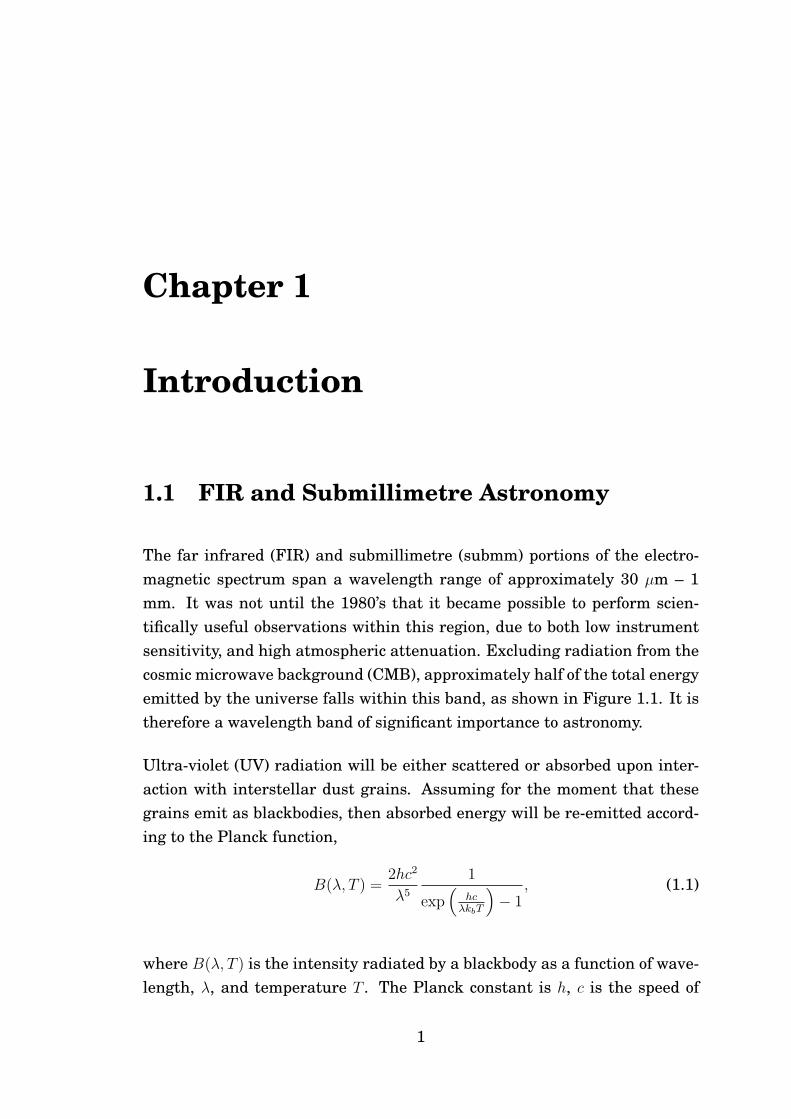
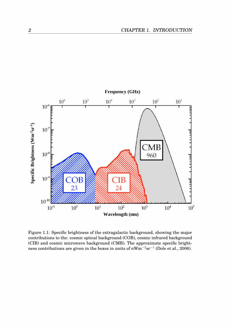
The far infrared (FIR) and submillimetre (submm) portions of the electro-magnetic spectrum span a wavelength range of approximately 30 µm – 1mm. It was not until the 1980’s that it became possible to perform scien-tifically useful observations within this region, due to both low instrumentsensitivity, and high atmospheric attenuation. Excluding radiation from thecosmic microwave background (CMB), approximately half of the total energyemitted by the universe falls within this band, as shown in Figure 1.1. It istherefore a wavelength band of significant importance to astronomy.
Ultra-violet (UV) radiation will be either scattered or absorbed upon inter-action with interstellar dust grains. Assuming for the moment that thesegrains emit as blackbodies, then absorbed energy will be re-emitted accord-ing to the Planck function,
B(λ, T ) =2hc2
λ5
1
exp(
hcλkbT
)− 1
, (1.1)
where B(λ, T ) is the intensity radiated by a blackbody as a function of wave-length, λ, and temperature T . The Planck constant is h, c is the speed of
1
2 CHAPTER 1. INTRODUCTION
Wavelength (µm)
Spec
ific
Bri
ghtn
ess
(Wm
-2sr
-1)
Frequency (GHz)
Figure 1.1: Specific brightness of the extragalactic background, showing the majorcontributions to the: cosmic optical background (COB), cosmic infrared background(CIB) and cosmic microwave background (CMB). The approximate specific bright-ness contributions are given in the boxes in units of nWm−2sr−1 (Dole et al., 2006).
1.1. FIR AND SUBMILLIMETRE ASTRONOMY 3
light, and kb is Boltzmann’s constant.
The Planck function peaks in the FIR/submm for sources with a temperatureof∼10–50 K. Cold cosmic dust is within this temperature range, making thiswaveband ideal for dust observations.
For optically thin dust sources, the observed flux density depends on bothdust temperature and density. This makes the determination of the sourcephysical parameters difficult, as the same observed brightness could be dueto a number of different combinations of parameters. In order to breakthis temperature/density degeneracy, a range of multi-wavelength measure-ments, which span the peak of the spectral energy distribution (SED), isrequired. If a good estimate of the peak cannot be made, then it is not possi-ble to determine with any accuracy the temperature of the source, and hencephysical conditions of the cloud.
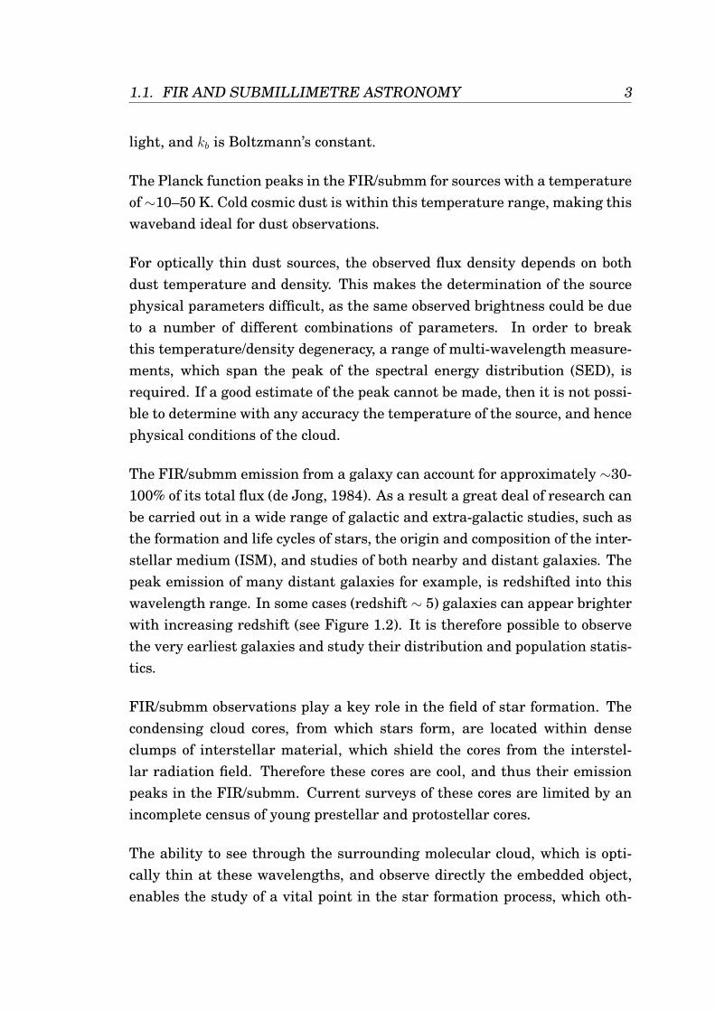
The FIR/submm emission from a galaxy can account for approximately ∼30-100% of its total flux (de Jong, 1984). As a result a great deal of research canbe carried out in a wide range of galactic and extra-galactic studies, such asthe formation and life cycles of stars, the origin and composition of the inter-stellar medium (ISM), and studies of both nearby and distant galaxies. Thepeak emission of many distant galaxies for example, is redshifted into thiswavelength range. In some cases (redshift ∼ 5) galaxies can appear brighterwith increasing redshift (see Figure 1.2). It is therefore possible to observethe very earliest galaxies and study their distribution and population statis-tics.
FIR/submm observations play a key role in the field of star formation. Thecondensing cloud cores, from which stars form, are located within denseclumps of interstellar material, which shield the cores from the interstel-lar radiation field. Therefore these cores are cool, and thus their emissionpeaks in the FIR/submm. Current surveys of these cores are limited by anincomplete census of young prestellar and protostellar cores.
The ability to see through the surrounding molecular cloud, which is opti-cally thin at these wavelengths, and observe directly the embedded object,enables the study of a vital point in the star formation process, which oth-
4 CHAPTER 1. INTRODUCTION
Figure 1.2: Galaxy spectrum in the submm/FIR region for a galaxy with luminosityof 1012L at redshifts of z = 0.1, 0.5, 1, 3, 5 from top to bottom respectively (Guider-doni et al., 1998).
1.1. FIR AND SUBMILLIMETRE ASTRONOMY 5
erwise could only be studied theoretically. Multi-wavelength observationsprovide the data required to determine the temperature and density of thesenewly forming stars, and thus derive their mass (see Section 2.4.2), as wellas information relating to the initial conditions of star formation.
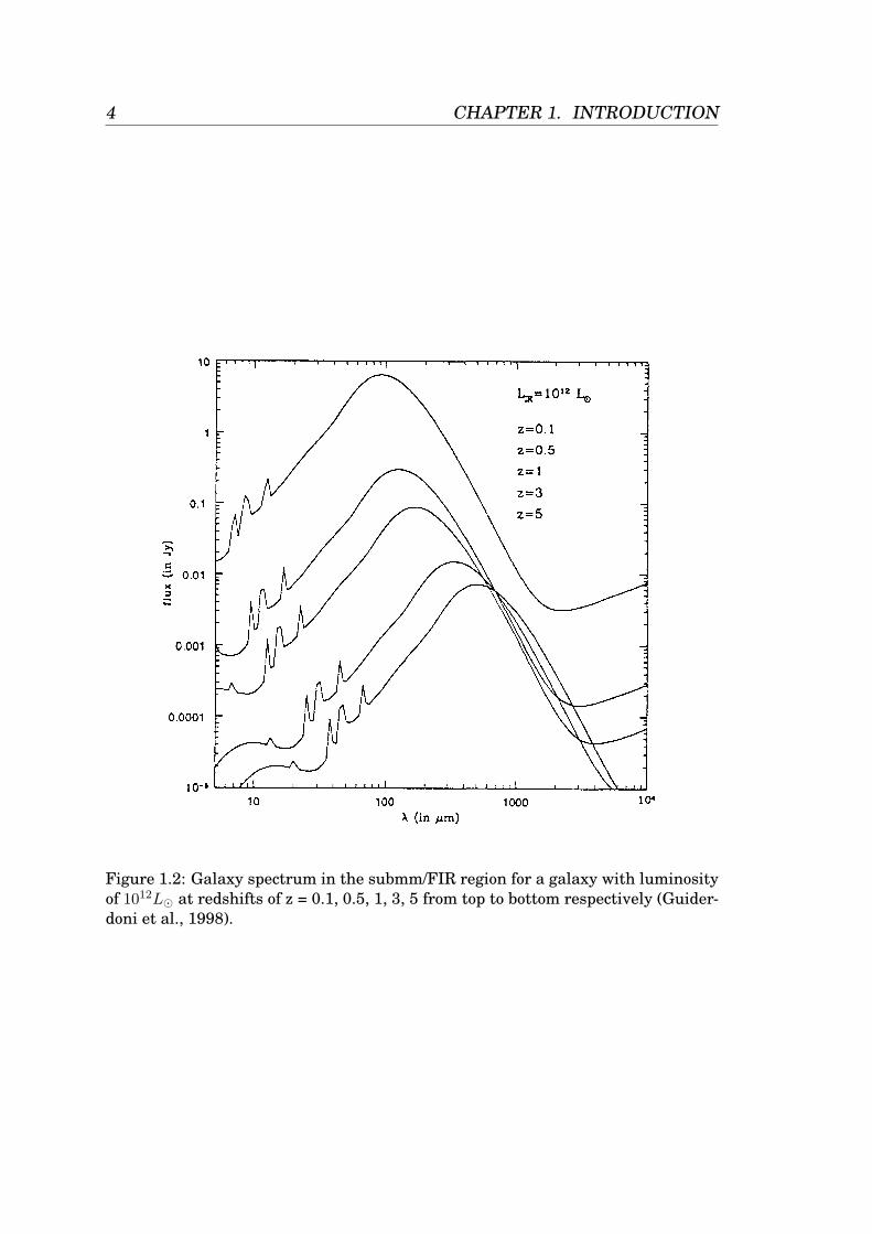
The FIR/submm waveband also contains a wide range of atomic, molecular,and fine structure line features. A sample spectrum from a ground basedsurvey is given in Figure 1.3. The emission and absorption features due tothe atmosphere are shown by the top line in the figure, and the astronomi-cal features are shown below. A high density of features can be clearly seen.This spectrum was obtained at the ground based Caltech Submillimetre Ob-servatory (CSO) in Hawaii.
Rest Frequency (GHz)700650
Ant
enna
Tem
pera
ture
(K)
0
-50
50
100
Figure 1.3: Sample spectrum in the FIR/submm band taken at the CSO. The topline is atmospheric emission/absorption, and the bottom line is the astronomicalspectrum (de Graauw et al., 2005).
Measurement of the gas emission provides physical information about theregion, such as gas abundances, density, temperature and kinematics. De-tection of various types of gas also help to characterise regions. The brightCO emission line for example, seen in Figure 1.3, is typically a tracer ofmolecular hydrogen, and thus molecular clouds.
6 CHAPTER 1. INTRODUCTION
1.1.1 Observing in the FIR and Submillimetre
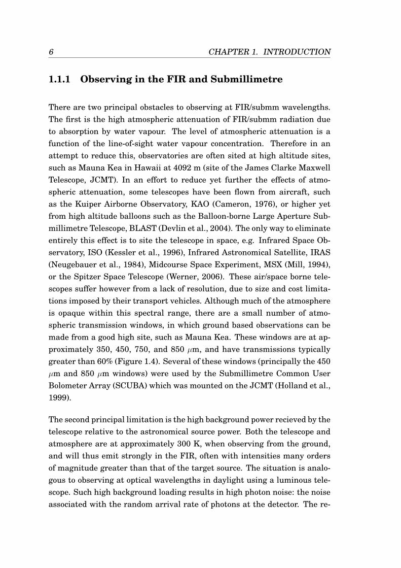
There are two principal obstacles to observing at FIR/submm wavelengths.The first is the high atmospheric attenuation of FIR/submm radiation dueto absorption by water vapour. The level of atmospheric attenuation is afunction of the line-of-sight water vapour concentration. Therefore in anattempt to reduce this, observatories are often sited at high altitude sites,such as Mauna Kea in Hawaii at 4092 m (site of the James Clarke MaxwellTelescope, JCMT). In an effort to reduce yet further the effects of atmo-spheric attenuation, some telescopes have been flown from aircraft, suchas the Kuiper Airborne Observatory, KAO (Cameron, 1976), or higher yetfrom high altitude balloons such as the Balloon-borne Large Aperture Sub-millimetre Telescope, BLAST (Devlin et al., 2004). The only way to eliminateentirely this effect is to site the telescope in space, e.g. Infrared Space Ob-servatory, ISO (Kessler et al., 1996), Infrared Astronomical Satellite, IRAS(Neugebauer et al., 1984), Midcourse Space Experiment, MSX (Mill, 1994),or the Spitzer Space Telescope (Werner, 2006). These air/space borne tele-scopes suffer however from a lack of resolution, due to size and cost limita-tions imposed by their transport vehicles. Although much of the atmosphereis opaque within this spectral range, there are a small number of atmo-spheric transmission windows, in which ground based observations can bemade from a good high site, such as Mauna Kea. These windows are at ap-proximately 350, 450, 750, and 850 µm, and have transmissions typicallygreater than 60% (Figure 1.4). Several of these windows (principally the 450µm and 850 µm windows) were used by the Submillimetre Common UserBolometer Array (SCUBA) which was mounted on the JCMT (Holland et al.,1999).
The second principal limitation is the high background power recieved by thetelescope relative to the astronomical source power. Both the telescope andatmosphere are at approximately 300 K, when observing from the ground,and will thus emit strongly in the FIR, often with intensities many ordersof magnitude greater than that of the target source. The situation is analo-gous to observing at optical wavelengths in daylight using a luminous tele-scope. Such high background loading results in high photon noise: the noiseassociated with the random arrival rate of photons at the detector. The re-
1.1. FIR AND SUBMILLIMETRE ASTRONOMY 7
Figure 1.4: Modelled atmospheric transmission at FIR wavelengths for a precip-itable water vapour level of 225 µm (Hayton, 2004).
sult is a degraded instrument sensitivity. The primary contribution to thishigh background comes from atmospheric emission, and is thus impossibleto overcome. Whilst clever data reduction methods do allow for the subtrac-tion of some sky effects, the only way to avoid the problem is again to sitethe telescope in space. Even so the sensitivity of a space telescope may stillbe limited by the background loading from emission by the telescope or op-tics. This can be minimised by cooling the optics to cryogenic temperatures,as was done for ISO and Spitzer, though this may not be practical or costeffective when dealing with telescopes with large apertures.
Observations in the submm/FIR are often made by ‘chopping’ (Figure 1.5).Here the telescope beam is moved alternatively between two positions onthe sky, commonly by the use of a moving secondary mirror. The telescopeobserves first an image of the sky plus source, and then just the sky. The skybackground image can then be subtracted from the source plus sky imageleaving solely source information. In addition to chopping an observation, atelescope is often “nodded”. When nodding, a telescope switches the on andoff source chop positions. Therefore, if there is any systematic differencebetween the two chop positions, such as a variation in the background fromthe telescope, then this contaminating signal can be removed.

8 CHAPTER 1. INTRODUCTION
Figure 1.5: Schematic showing beam positions within a chopped observation in bothnod positions (Harwit, 2001).
Confusion noise may also affect the sensitivity of an observation. This noiseis due to contaminating sources within the telescope beam, due to emissionfrom either galactic cirrus, or background galaxies. This can be reduced byincreasing the angular resolution of the telescope, thus reducing the beamsize. The origin of confusion noise means than it cannot be integrated downthrough longer observing times. It therefore determines the ultimate limitto the sensitivity of a telescope of given size.
Recently a number of instruments designed to carry out large area imag-ing surveys at submm/FIR wavelengths without chopping have been devel-oped. These include BOLOCAM (Mauskopf et al., 2000), BLAST (Devlinet al., 2004), SCUBA-2 (Audley et al., 2003), LABOCA (Kreysa et al., 2003),Planck-HFI (Lamarre et al., 2003), and the PACS (Poglitsch et al., 2005) andSPIRE (Griffin et al., 2006) instruments on board the ESA Herschel spaceobservatory (Pilbratt, 2005). Such ‘scanning’ instruments are no longer lim-ited in observable source size scale by their chop throw. These systems alsoobserve the source for the entire observation time, thus increasing the ob-serving efficiency by a factor of 2, and the sensitivity by a factor of
√2. Such
instruments are however more sensitive to 1/f noise fluctuations, arisingfrom atmospheric variations, or from within the detection system.
1.2. HERSCHEL 9
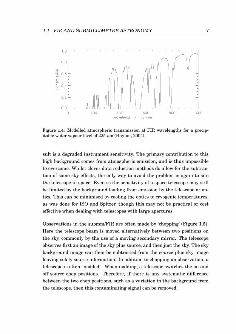
The definition of 1/f noise is a noise whose power spectrum decreases as oneover the frequency until it meets the white noise floor, en (Figure 1.6). Ittherefore contains greater power at low frequencies, resulting in long timescale noise drifts. Longer integration time (t) of 1/f noise will not provide theexpected
√t improvement in signal to noise ratio, and will result in a higher
than expected timeline variance, as compared to white noise. 1/f noise canbe characterised by a knee frequency, fk. This is defined as the frequency atwhich the noise voltage spectral density is a factor of
√2 times greater than
that of the white noise voltage spectral density.
noise power
fk
en
√2en
frequency
Figure 1.6: Schematic 1/f noise power spectrum illustrating the definition of fk.
1.2 Herschel
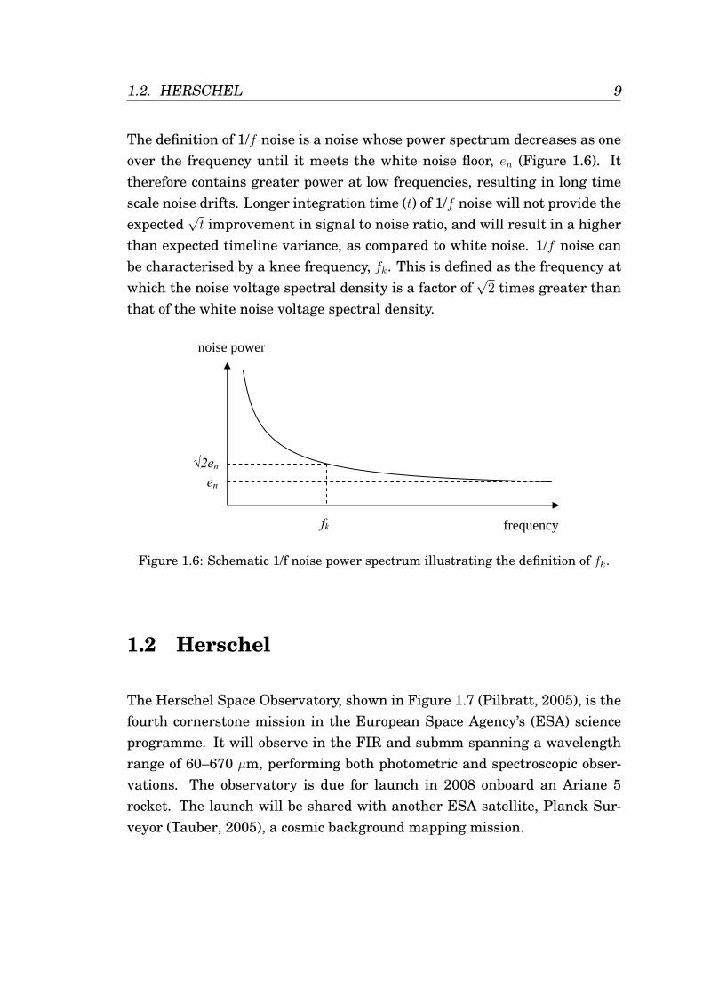
The Herschel Space Observatory, shown in Figure 1.7 (Pilbratt, 2005), is thefourth cornerstone mission in the European Space Agency’s (ESA) scienceprogramme. It will observe in the FIR and submm spanning a wavelengthrange of 60–670 µm, performing both photometric and spectroscopic obser-vations. The observatory is due for launch in 2008 onboard an Ariane 5rocket. The launch will be shared with another ESA satellite, Planck Sur-veyor (Tauber, 2005), a cosmic background mapping mission.
10 CHAPTER 1. INTRODUCTION
Figure 1.7: Computer generated image of the Herschel Observatory (Pilbratt, 2005).
1.2. HERSCHEL 11
1.2.1 Herschel Science
Herschel will be the first facility to observe in the FIR and submm wave-bands from space, providing high sensitivity observations at relatively highspatial resolution, compared to previous space-borne observatories in thiswavelength region. Herschel effectively targets the cold universe, with awavelength range encompassing both the brightest atomic and molecularemission lines for sources at temperatures from 10 to a few hundred K,and the peak emission from black-body sources at temperatures of 10–50K. High redshift galaxies will also have their peak emission redshifted intothe ‘prime’ Herschel band, providing the ability to study some of the earli-est proto-galaxies. Some prime science goals for Herschel include (Pilbratt,2005):
• detailed investigations of the formation and evolution of galaxy bulgesand elliptical galaxies in the first third of the present age of the Uni-verse;
• detailed studies of the physics and chemistry of the interstellar mediumin galaxies, both locally in our own Galaxy as well as in external galax-ies;
• the physical and chemical processes involved in star formation andearly stellar evolution in our own Galaxy;
• high resolution spectroscopy of a number of comets and the atmospheresof the cool outer planets and their satellites.
Observations made by Herschel will complement those of other forthcomingfacilities, such as SCUBA-2 and ALMA, by providing high sensitivity lownoise measurements in a similar wavelength range. They will also comple-ment current Spitzer studies.
12 CHAPTER 1. INTRODUCTION
1.2.2 The Herschel Spacecraft
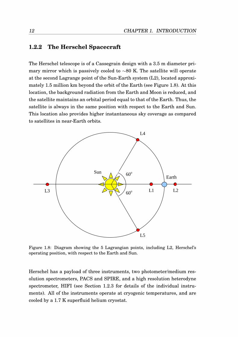
The Herschel telescope is of a Cassegrain design with a 3.5 m diameter pri-mary mirror which is passively cooled to ∼80 K. The satellite will operateat the second Lagrange point of the Sun-Earth system (L2), located approxi-mately 1.5 million km beyond the orbit of the Earth (see Figure 1.8). At thislocation, the background radiation from the Earth and Moon is reduced, andthe satellite maintains an orbital period equal to that of the Earth. Thus, thesatellite is always in the same position with respect to the Earth and Sun.This location also provides higher instantaneous sky coverage as comparedto satellites in near-Earth orbits.
Sun Earth
L1 L2
L5
L4
L3
60o
60o
Figure 1.8: Diagram showing the 5 Lagrangian points, including L2, Herschel’soperating position, with respect to the Earth and Sun.
Herschel has a payload of three instruments, two photometer/medium res-olution spectrometers, PACS and SPIRE, and a high resolution heterodynespectrometer, HIFI (see Section 1.2.3 for details of the individual instru-ments). All of the instruments operate at cryogenic temperatures, and arecooled by a 1.7 K superfluid helium cryostat.
1.2. HERSCHEL 13
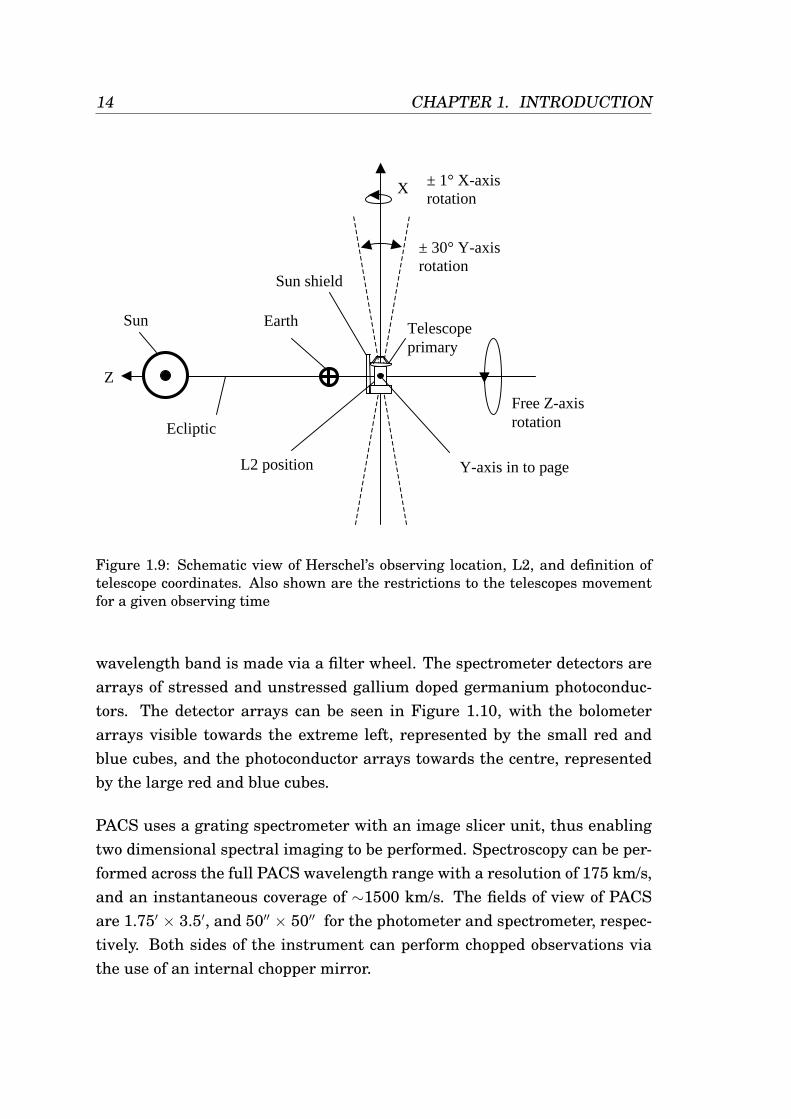
The spacecraft is protected from the heat of the Sun by a Sun shield. Thisshield must be kept facing the Sun at all times to avoid excess boil-off ofthe on-board cryogens, prevent stray light from entering the system, andmaintain thermal stability. This limits the range of satellite movement, andconsequently the observable area of sky at a given point in time. With refer-ence to the telescope coordinates shown in Figure 1.9, the satellite is free torotate about the Z axis, and has ±30 movement about the Y axis, dictatedby the constraint that the Sun must not shine on the telescope or spacecraftbus. The telescope also has a roll angle constraint of ±1. This movementis generally considered to be negligible and does not appear in optimisationstudies of the observing modes.
These operational restrictions mean that at any one time the telescope canpoint to a position within a 60 wide strip of the sky. The observable stripvaries throughout the year as the Earth and telescope orbit the Sun. Theobserving strip will pass over all parts of the sky once during a 6 monthhalf-orbit.
The mission is scheduled to last a minimum of 3 years, and have a total costof ∼e1 billion, resulting in an observing time cost of ∼e1 million per day.This cost includes both the spacecraft and instruments. Approximately 2/3of the observing time will be available to the general community, with theother third being allocated as guaranteed time to the instrument buildersand the Herschel Science Centre (HSC) team.
1.2.3 Instruments
PACS
PACS, the Photodetector Array Camera and Spectrometer (Poglitsch et al.,2005), contains both a three colour photometer and a low–medium resolu-tion imaging spectrometer, observing over a wavelength range of ∼60–210µm. The photometer uses two filled silicon bolometer arrays containing 16 ×32 and 32 × 64 pixels. Simultaneous operation of both arrays is possible, ob-serving in the 60–90 or 90–130, and 130–210 µm bands. The change in short
14 CHAPTER 1. INTRODUCTION
Telescope primary
L2 position
Ecliptic
Earth Sun
Z
X
Sun shield
± 30° Y-axis rotation
Free Z-axis rotation
± 1° X-axis rotation
Y-axis in to page
Figure 1.9: Schematic view of Herschel’s observing location, L2, and definition oftelescope coordinates. Also shown are the restrictions to the telescopes movementfor a given observing time
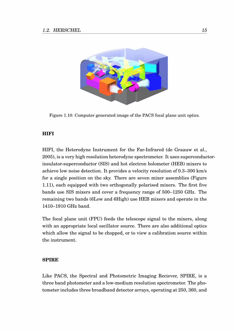
wavelength band is made via a filter wheel. The spectrometer detectors arearrays of stressed and unstressed gallium doped germanium photoconduc-tors. The detector arrays can be seen in Figure 1.10, with the bolometerarrays visible towards the extreme left, represented by the small red andblue cubes, and the photoconductor arrays towards the centre, representedby the large red and blue cubes.
PACS uses a grating spectrometer with an image slicer unit, thus enablingtwo dimensional spectral imaging to be performed. Spectroscopy can be per-formed across the full PACS wavelength range with a resolution of 175 km/s,and an instantaneous coverage of ∼1500 km/s. The fields of view of PACSare 1.75′ × 3.5′, and 50′′ × 50′′ for the photometer and spectrometer, respec-tively. Both sides of the instrument can perform chopped observations viathe use of an internal chopper mirror.
1.2. HERSCHEL 1516 Goran L. Pilbratt
Figure 3. Computer rendering of the PACS focal plane unit op-tics. The bolometer arrays are visible towards the extreme left,the photoconductor arrays are the large red and blue ‘cubes’respectively.
PACS has three photometric bands with R∼ 2. Theshort wavelength ‘blue’ array covers the 60−90 and 90−130µm bands, while the ‘red’ array covers the 130−210 µmband. In photometric mode one of the ‘blue’ bands and the‘red’ band are observed simultaneously. The two bolome-ter arrays both fully sample the same 1.′75×3.′5 field ofview on the sky, and provide a predicted point source de-tection limit of ∼ 3 mJy (5σ, 1 hr) in all three bands.An internal 3He sorption cooler will provide the 300mKenvironment needed by the bolometers.
For spectroscopy PACS covers 57−210 µm in threecontiguous bands, providing a velocity resolution in therange 150−200 km−1 and an instantaneous coverage of∼ 1500 km−1. The two Ge:Ga arrays are appropriatelystressed and operated at slightly different temperatures –cooled by being ‘strapped’ to the liquid helium – in or-der to optimise sensitivity for their respective wavelengthcoverage. The predicted point source detection limit is∼ 3×10⁻¹⁸Wm−2 (5σ, 1 hr) over most of the band, risingto ∼ 8×10⁻¹⁸Wm−2 for the shortest wavelengths.
3.2.2. SPIRE - a camera and spectrometer
SPIRE (for a full description see Griffin et al. 2001 =this volume) is a camera and low to medium resolutionspectrometer for wavelengths above ∼ 200 µm (Fig. 4). Itcomprises an imaging photometer and a Fourier Trans-form Spectrometer (FTS), both of which use bolometerdetector arrays. There are a total of five arrays, three ded-icated for photometry and two for spectroscopy. All em-ploy ‘spider-web’ bolometers with NTD Ge temperaturesensors, with each pixel being fed by a single-mode 2Fλfeedhorn, and JFET readout electronics. The bolometersare cooled to 300mK by an internal 3He sorption cooler.
SPIRE has been designed to maximise mapping speed.In its broadband (R∼ 3) photometry mode it simultane-ously images a 4′×8′ field on the sky in three colours cen-tred on 250, 350, and 500 µm. Since the telescope beam
Figure 4. The SPIRE photometer layout. The internal 3Hesorption cooler provides the 300 mK operating temperature.
is not instantaneously fully sampled, it will be requiredeither to scan along a preferred angle, or to ‘fill in’ by ‘jig-gling’ with the internal beam steering mirror. The SPIREpoint source sensitivity for mapping is predicted to be inthe range 7−9 mJy (5σ, 1 hr). Since the confusion limitfor extragalactic surveys is estimated to lie in the range10−20 mJy, SPIRE will be able to map ∼ 0.5 square de-gree on the sky per day to its confusion limit.
The SPIRE spectrometer is based on a Mach-Zenderconfiguration with novel broad-band beam dividers. Bothinput ports are used at all times, the signal port acceptsthe beam from the telescope while the second port acceptsa signal from a calibration source, the level of which ischosen to balance the power from the telescope in thesignal beam. The two output ports have detector arraysdedicated for 200−300 and 300−600 µm respectively. Themaximum resolution will be in the range 100−1000 at awavelength of 250 µm, and the field of view ∼ 2.6′.
3.2.3. HIFI - a very high resolution spectrometer
HIFI (for a full description see de Graauw & Helmich2001 = this volume) is a very high resolution heterodynespectrometer. It offers velocity resolution in the range0.3−300 kms−1, combined with low noise detection usingsuperconductor-insulator-superconductor (SIS) and hot elec-tron bolometer (HEB) mixers. HIFI is not an imaging in-strument, it provides a single pixel on the sky.
The focal plane unit (FPU, Fig. 5), houses seven mixerassemblies, each one equipped with two orthogonally po-larised mixers. Bands 1−5 utilise SIS mixers that togethercover approximately 500−1250 GHz without any gaps inthe frequency coverage. Bands 6Low and 6High utiliseHEB mixers, and together target the 1410−1910 band.The FPU also houses the optics that feeds the mixers the
Figure 1.10: Computer generated image of the PACS focal plane unit optics.
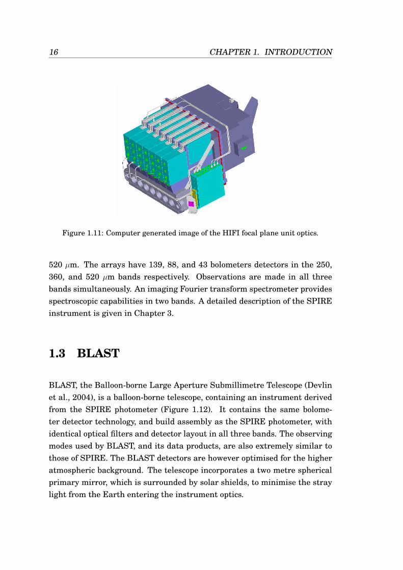
HIFI
HIFI, the Heterodyne Instrument for the Far-Infrared (de Graauw et al.,2005), is a very high resolution heterodyne spectrometer. It uses superconductor-insulator-superconductor (SIS) and hot electron bolometer (HEB) mixers toachieve low noise detection. It provides a velocity resolution of 0.3–300 km/sfor a single position on the sky. There are seven mixer assemblies (Figure1.11), each equipped with two orthogonally polarised mixers. The first fivebands use SIS mixers and cover a frequency range of 500–1250 GHz. Theremaining two bands (6Low and 6High) use HEB mixers and operate in the1410–1910 GHz band.
The focal plane unit (FPU) feeds the telescope signal to the mixers, alongwith an appropriate local oscillator source. There are also additional opticswhich allow the signal to be chopped, or to view a calibration source withinthe instrument.
SPIRE
Like PACS, the Spectral and Photometric Imaging Reciever, SPIRE, is athree band photometer and a low-medium resolution spectrometer. The pho-tometer includes three broadband detector arrays, operating at 250, 360, and
16 CHAPTER 1. INTRODUCTIONThe Herschel Mission, Scientific Objectives, and this Meeting 17
Figure 5. The HIFI focal plane unit with the seven mixer as-semblies in the foreground.
signal from the telescope and combines it with the ap-propriate local oscillator (LO) signal, as well as providesa chopper and the capability to view internal calibrationloads.
The LO signal is generated by a source unit locatedin the spacecraft service module (SVM, see Section 4). Bymeans of waveguides it is fed to the LO unit, located on theoutside of the cryostat vessel, where it is amplified, mul-tiplied and subsequently quasioptically fed to the FPU.The SVM also houses the complement of autocorrelatorand acousto-optical backend spectrometers.
4. Spacecraft and orbit
The Herschel configuration shown in Fig. 1 envisages apayload module based on the now well proven ISO cryo-stat technology. This configuration has been used to es-tablish payload interfaces and study mission design. Itis modular, consisting of a payload module (PLM, Col-laudin et al. 2000) comprising the superfluid helium cryo-stat – housing the optical bench with the instrument FPUs(Fig. 6) – which supports the telescope, star trackers, andsome payload associated equipment; and the service mod-ule (SVM), which provides the ‘infrastructure’ and housesthe ‘warm’ payload electronics.
This Herschel concept measures 9.3m in height, 4.5min width, and has an approximate launch mass of 3000kg.The 3.5 m diameter Herschel telescope is protected by thesunshade, and will cool passively to around 80K. The Her-schel science payload focal plane units are housed insidethe cryostat, which contains superfluid helium at below1.7K. Fixed solar panels on the sunshade deliver in excessof 1 kW power. Three startrackers in a skewed configu-ration and the local oscillator unit for the heterodyne in-strument are visible on the outside of the cryostat vacuumvessel.
Figure 6. Exploded view of the upper part of the Herschel pay-load module, showing the three instrument focal plane units onthe optical bench on top of the superfluid helium tank insidethe cryostat vacuum vessel. (Courtesy Astrium.)
An Ariane 5 launcher (Fig. 7 left), shared by the ESAcosmic microwave background mapping mission Planckand Herschel, will inject both satellites into a transfertrajectory towards the second Lagrangian point (L2) inthe Sun-Earth system. They will then separate from thelauncher, and subsequently operate independently fromorbits of different amplitude around L2.
Figure 7. Left: A single Ariane 5 launcher will place both Her-schel and Planck in transfer trajectories towards L2. Right: L2is situated 0.01 AU from the Earth in the anti-sunward direc-tion, providing a thermally stable favourable vantage point forperforming observations.
The L2 point is situated 1.5 million km away from theEarth in the anti-sunward direction (Fig. 7 right). It of-fers a stable thermal environment with good sky visibility.Since Herschel will be in a large orbit around L2, whichhas the advantage of not costing any ‘orbit injection’ ∆v,its distance to the Earth will vary between 1.2 and 1.8million km. The transfer to the operational orbit will lastapproximately 4 months. After cooldown and outgassinghave taken place, it is planned to use this time for commis-
Figure 1.11: Computer generated image of the HIFI focal plane unit optics.
520 µm. The arrays have 139, 88, and 43 bolometers detectors in the 250,360, and 520 µm bands respectively. Observations are made in all threebands simultaneously. An imaging Fourier transform spectrometer providesspectroscopic capabilities in two bands. A detailed description of the SPIREinstrument is given in Chapter 3.
1.3 BLAST
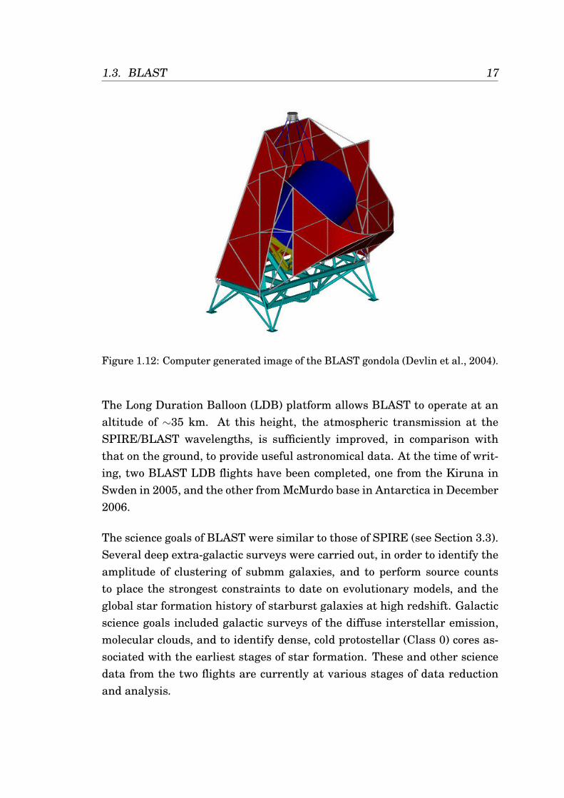
BLAST, the Balloon-borne Large Aperture Submillimetre Telescope (Devlinet al., 2004), is a balloon-borne telescope, containing an instrument derivedfrom the SPIRE photometer (Figure 1.12). It contains the same bolome-ter detector technology, and build assembly as the SPIRE photometer, withidentical optical filters and detector layout in all three bands. The observingmodes used by BLAST, and its data products, are also extremely similar tothose of SPIRE. The BLAST detectors are however optimised for the higheratmospheric background. The telescope incorporates a two metre sphericalprimary mirror, which is surrounded by solar shields, to minimise the straylight from the Earth entering the instrument optics.
1.3. BLAST 17
Figure 1.12: Computer generated image of the BLAST gondola (Devlin et al., 2004).
The Long Duration Balloon (LDB) platform allows BLAST to operate at analtitude of ∼35 km. At this height, the atmospheric transmission at theSPIRE/BLAST wavelengths, is sufficiently improved, in comparison withthat on the ground, to provide useful astronomical data. At the time of writ-ing, two BLAST LDB flights have been completed, one from the Kiruna inSwden in 2005, and the other from McMurdo base in Antarctica in December2006.
The science goals of BLAST were similar to those of SPIRE (see Section 3.3).Several deep extra-galactic surveys were carried out, in order to identify theamplitude of clustering of submm galaxies, and to perform source countsto place the strongest constraints to date on evolutionary models, and theglobal star formation history of starburst galaxies at high redshift. Galacticscience goals included galactic surveys of the diffuse interstellar emission,molecular clouds, and to identify dense, cold protostellar (Class 0) cores as-sociated with the earliest stages of star formation. These and other sciencedata from the two flights are currently at various stages of data reductionand analysis.
18 CHAPTER 1. INTRODUCTION
1.4 Bolometers
Bolometers are cryogenic detectors often used to detect submm/FIR radia-tion (see Richards, 1994 for a review). They are used in this wavelengthrange as other continuum detectors, such as photoconductors, are unable towork at wavelengths greater than ∼ 200µm. Heterodyne mixers are not usedas they unable to provide the bandwidth required to perform broad-bandphotometry, and have a lower sensitivity at FIR/submm wavelengths. It isalso relatively easy now to build large arrays of bolometers, thus improvingobserving efficiency. This section summarises some of the key points fromthe papers by Mather (1982), Richards (1994), and Sudiwala et al. (1992).
A bolometer works by absorbing incoming electromagnetic power, causing arise in temperature of the detector. This temperature change results in achange of resistance of the detector material, which is then read out as avariation in detector voltage. The amplitude of this voltage change is pro-portional to the power absorbed by the detector.
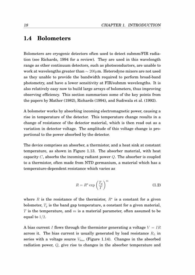
The device comprises an absorber, a thermistor, and a heat sink at constanttemperature, as shown in Figure 1.13. The absorber material, with heatcapacity C, absorbs the incoming radiant power Q. The absorber is coupledto a thermistor, often made from NTD germanium, a material which has atemperature-dependent resistance which varies as
R = R? exp
(TgT
)m
(1.2)
where R is the resistance of the thermistor, R? is a constant for a givenbolometer, Tg is the band gap temperature, a constant for a given material,T is the temperature, and m is a material parameter, often assumed to beequal to 1/2.
A bias current I flows through the thermistor generating a voltage V = IR
across it. The bias current is usually generated by load resistance RL inseries with a voltage source Vbias (Figure 1.14). Changes in the absorbedradiation power, Q, give rise to changes in the absorber temperature and
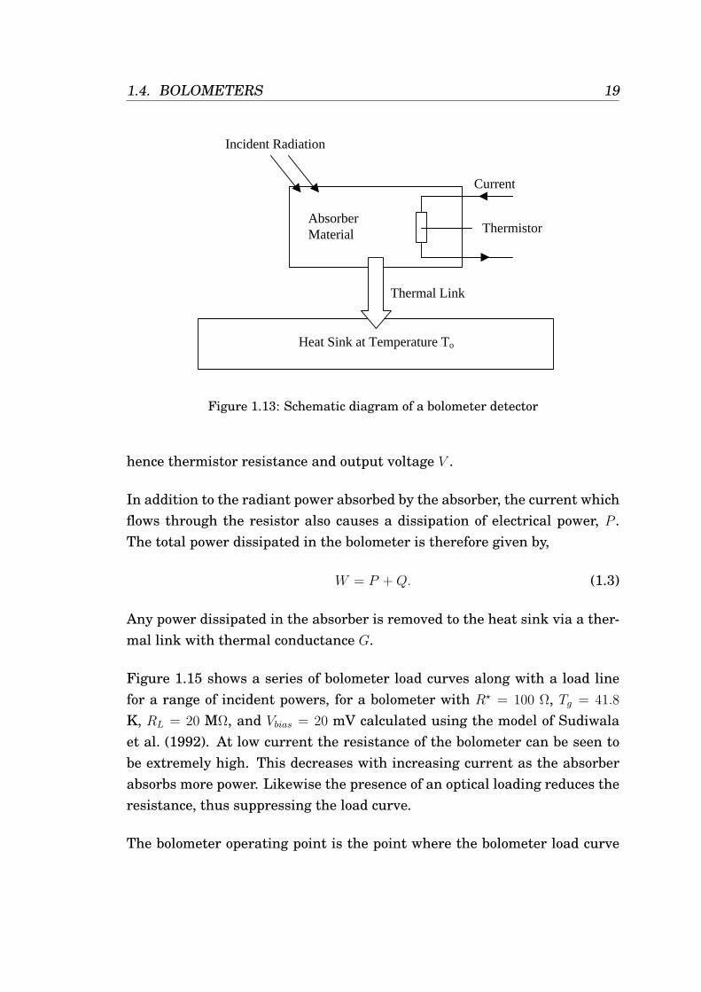
1.4. BOLOMETERS 19
Heat Sink at Temperature To
Absorber Material
Incident Radiation
Thermal Link
Current
Thermistor
Figure 1.13: Schematic diagram of a bolometer detector
hence thermistor resistance and output voltage V .
In addition to the radiant power absorbed by the absorber, the current whichflows through the resistor also causes a dissipation of electrical power, P .The total power dissipated in the bolometer is therefore given by,
W = P +Q. (1.3)
Any power dissipated in the absorber is removed to the heat sink via a ther-mal link with thermal conductance G.
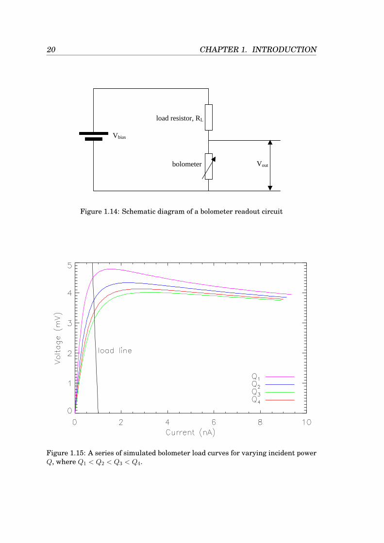
Figure 1.15 shows a series of bolometer load curves along with a load linefor a range of incident powers, for a bolometer with R? = 100 Ω, Tg = 41.8
K, RL = 20 MΩ, and Vbias = 20 mV calculated using the model of Sudiwalaet al. (1992). At low current the resistance of the bolometer can be seen tobe extremely high. This decreases with increasing current as the absorberabsorbs more power. Likewise the presence of an optical loading reduces theresistance, thus suppressing the load curve.
The bolometer operating point is the point where the bolometer load curve
20 CHAPTER 1. INTRODUCTION
Vout bolometer
load resistor, RL
Vbias
Figure 1.14: Schematic diagram of a bolometer readout circuit
Figure 1.15: A series of simulated bolometer load curves for varying incident powerQ, where Q1 < Q2 < Q3 < Q4.
1.4. BOLOMETERS 21
(V I curve) crosses the load line, given by Equation 1.4.
V = Vbias − IRL (1.4)
In most cases the optical loading on a bolometer is dominated by the back-ground radiation. Therefore when a signal power background power ispresent, the departure of the load curve from its normal shape can be re-garded as negligible. In this instance the bolometer responds in a linearfashion, as defined by its responsivity S,
S =∆V
∆Q. (1.5)
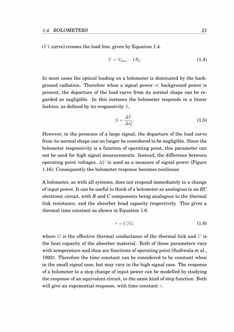
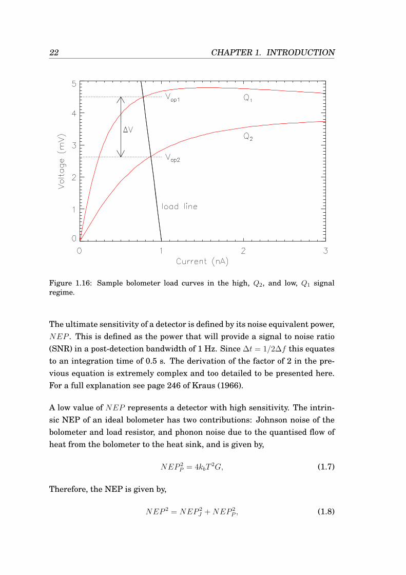
However, in the presence of a large signal, the departure of the load curvefrom its normal shape can no longer be considered to be negligible. Since thebolometer responsivity is a function of operating point, this parameter cannot be used for high signal measurements. Instead, the difference betweenoperating point voltages, ∆V is used as a measure of signal power (Figure1.16). Consequently the bolometer response becomes nonlinear.
A bolometer, as with all systems, does not respond immediately to a changeof input power. It can be useful to think of a bolometer as analogous to an RCelectronic circuit, with R and C components being analogous to the thermallink resistance, and the absorber head capacity respectively. This gives athermal time constant as shown in Equation 1.6.
τ = C/G, (1.6)
where G is the effective thermal conductance of the thermal link and C isthe heat capacity of the absorber material. Both of these parameters varywith temperature and thus are functions of operating point (Sudiwala et al.,1992). Therefore the time constant can be considered to be constant whenin the small signal case, but may vary in the high signal case. The responseof a bolometer to a step change of input power can be modelled by studyingthe response of an equivalent circuit, to the same kind of step function. Bothwill give an exponential response, with time constant τ .
22 CHAPTER 1. INTRODUCTION
Figure 1.16: Sample bolometer load curves in the high, Q2, and low, Q1 signalregime.
The ultimate sensitivity of a detector is defined by its noise equivalent power,NEP . This is defined as the power that will provide a signal to noise ratio(SNR) in a post-detection bandwidth of 1 Hz. Since ∆t = 1/2∆f this equatesto an integration time of 0.5 s. The derivation of the factor of 2 in the pre-vious equation is extremely complex and too detailed to be presented here.For a full explanation see page 246 of Kraus (1966).
A low value of NEP represents a detector with high sensitivity. The intrin-sic NEP of an ideal bolometer has two contributions: Johnson noise of thebolometer and load resistor, and phonon noise due to the quantised flow ofheat from the bolometer to the heat sink, and is given by,
NEP 2P = 4kbT
2G, (1.7)
Therefore, the NEP is given by,
NEP 2 = NEP 2J +NEP 2
P , (1.8)
1.5. CHAPTER SUMMARY 23
where NEPJ is the Johnson noise component and NEPP is the phonon noisecomponent. Since the two sources of noise are uncorrelated they are summedin quadrature. The specific form of NEPJ is derived in Mather (1982).
In addition to the phonon and Johnson noise, a bolometer is also affected byother forms of noise. The most significant is photon noise, which arises fromthe quantum nature of the incident radiation. Readout electronics are alsoa source of noise in any working system.
Another significant source of noise when operating a bolometer device canbe thermal fluctuations. The temperature dependent nature of a bolometermeans that a stable heat sink is essential. The parameters derived in thethermal modelling of a bolometer (Sudiwala et al., 1992) are almost all tem-perature dependant, and are often specific to a single detector. As a resultthe scale of error arising from a temperature fluctuation may be differentacross a bolometer array. The NEP contribution due to thermal variations isgiven by,
NEP 2T =
G2STη2
, (1.9)
where ST is the spectral intensity of fluctuation in the temperature of theheat sink, and η is the bolometer absorptivity (Richards, 1994).
Both thermal variations in the heat sink and electronic noise are expectedto have a 1/f noise power spectrum.
1.5 Chapter Summary
This chapter has introduced and summarised FIR/submm astronomy, andthe techniques by which it is performed. An overview of the Herschel andBLAST projects has also been given, including details of the PACS and HIFIinstruments on board Herschel. Finally, a brief review of bolometer opera-tion has been presented.
24 CHAPTER 1. INTRODUCTION
1.6 Outline of this Thesis
In this thesis I describe the results of an investigation of various systematicaspects of the Herschel/SPIRE photometer system, and their impact on dataquality and observing efficiency. These include the observing modes usedto collect the data, as well as sources of noise. This has been achieved bydeveloping and using a new, highly detailed and realistic, software simulatorof the SPIRE photometer.
The investigations of the instrument systematics have been used to opti-mise the nominal instrument observing parameters. This work was thenextended to investigate the effect on planned observations of targets withinour galaxy, including the extraction of large diffuse structure in the presenceof 1/f noise, and the study of radial profiles of prestellar cores.
In addition I present the analysis of some data from the BLAST experiment.Specifically, I report the first observations of the Cassiopeia A supernovaremnant made at 250, 360, and 520 µm. I discuss their relevance and contri-bution to the on-going debate about the dominant source of dust productionin the galaxy.
The specific goals of this work were to:
• develop and test a highly realistic software instrument simulator forthe Herschel/SPIRE photometer;
• investigate and optimise the SPIRE photometer observing modes;
• study the systematics which will affect Herschel observations of astro-nomical sources within our galaxy.
• determine, using BLAST data, the quantity of dust contained in theCassiopeia A supernova remnant;
Chapter 2 contains an introduction to the physical properties of dust, witha specific focus on their relevance, and consequences, in terms of FIR andsubmm astronomy. The next chapter covers the SPIRE instrument in more
1.6. OUTLINE OF THIS THESIS 25
detail. The system hardware and observing modes are described. Chapter4 describes the architecture and operation of the SPIRE photometer simu-lator, including information on the modelling of hardware, and sources oferror. Following this, Chapter 5 deals with the verification of the simula-tor output, and considers the data reduction processes required to turn thesimulator output timelines into a useful format for data analysis. Chapter6 outlines the optimisation of the SPIRE observing modes through use ofthe simulator, and defines the recommended nominal observing parameters.The next chapter contains the data analysis, and conclusions, of the Cas-siopeia A BLAST observations. Chapter 8 describes an investigation of theimpact of SPIRE instrument systematics on observations of galactic sources.This deals with the recovery of sources of arbitrary scale, and structure, bothin a confused and unconfused environment. Finally, Chapter 9 summarisesthe conclusions of the work in this thesis, and discusses future work andextensions to the current simulator.

26 CHAPTER 1. INTRODUCTION
Chapter 2
Dust in the Interstellar Medium
Dust may constitute only ∼1% of the interstellar medium (ISM), but it playsan extremely important role in its astrophysics. It is crucial in the chemistry,opacity, and thermal balance of the ISM, and governs the processes by whichstars form.
In this chapter, I introduce the ISM, and the cycle by which dust is injectedand removed from it. I look at some of the main processes involved, includingdust grain creation, and star formation. The observational properties of dustare also reviewed, with particular attention paid to the FIR and submm, andto topics that are relevant to the work contained in subsequent chapters ofthis thesis.
2.1 The Interstellar Medium
The ISM is made up of many components, at different temperatures and indifferent phases (atomic, molecular, and ionized). Components include dust,high energy particles, and magnetic fields. The most abundant componenthowever is gas, mostly neutral atomic hydrogen (HI), with an average num-ber density of nH ∼ 105 H atoms m−3, and temperature of ∼100 K (Evans,1994). The density and temperature are by no means uniform however.
27
28 CHAPTER 2. DUST IN THE INTERSTELLAR MEDIUM
Regions of higher density exist, made up largely of molecular hydrogen (H2).These are known as molecular clouds, and can have number densities of H2
of up to 1010 molecules m−3 (Evans, 1994).
The number density of interstellar dust grains is also higher in molecularclouds than in the surrounding ISM. Interstellar dust grains are tiny par-ticles composed of heavy elements, mainly carbon and oxygen, which areinjected into the ISM by stars in the late stages of their evolution. It is thisdust that enables a great deal of the interstellar chemistry to occur: it ab-sorbs the high energy UV radiation which might otherwise cause moleculardissociation, and it also acts as a substrate for the formation of H2 molecules.In dense clouds, grains can also acquire a mantle, formed from material con-densed out of the gas phase. Hence, a lower hydrogen molecular numberdensity is observed for a given cloud mass (Whittet, 2003).
Dust absorption also shields the inner parts of the molecular clouds, allowingthem to cool and fragment, finally forming stars. The absorption efficiency ofthe dust allows gas clouds to cool and fragment into stars. The dust opacityis also thought to be responsible for stopping the collapse of the core duringstar formation. A supercritical core will collapse isothermally until suchtime that the density is sufficiently high that it becomes optically thick. Atthis point the core will collapse adiabatically, until the internal pressure ofthe core becomes sufficient to support it against further collapse (Ferrara,2003). The point at which the material becomes optically thick is a functionof the dust opacity.
Cosmic dust plays a vital role in the thermodynamics, chemistry, and phys-ical processes which occur in the ISM. It is observed around active galacticnuclei, the early and late stages of stellar evolution, as well as being funda-mental for planet formation (Whittet, 2003).
2.1.1 The Dust Cycle
The elemental composition of the primordial universe (∼13.7 Gyr ago) wasdominated by hydrogen. In addition, significant amounts of helium, and
2.2. THE ORIGIN OF DUST IN THE ISM 29
trace amounts of lithium were also formed. The fractional compositions bymass of hydrogen, helium, and the sum of all other heavier elements, arecommonly denoted as X, Y, and Z respectively. The fractions in the primor-dial universe are estimated to be Xp ' 0.76, Yp ' 0.24, Zp ' 0.00 (Whittet,2003). Zp is not identically zero, but is too small to be accounted for in thesefigures.
This material eventually formed galaxies and the first generation of stars,within which nuclear processing lead to the synthesis of heavier elements.These stars subsequently injected these newly formed elements into theISM, via stellar winds or through supernovae (SNe). Successive generationsof stars continued this enrichment of the ISM, leading to the current fractionof heavy elements seen today, Z' 0.02 (Whittet, 2003).
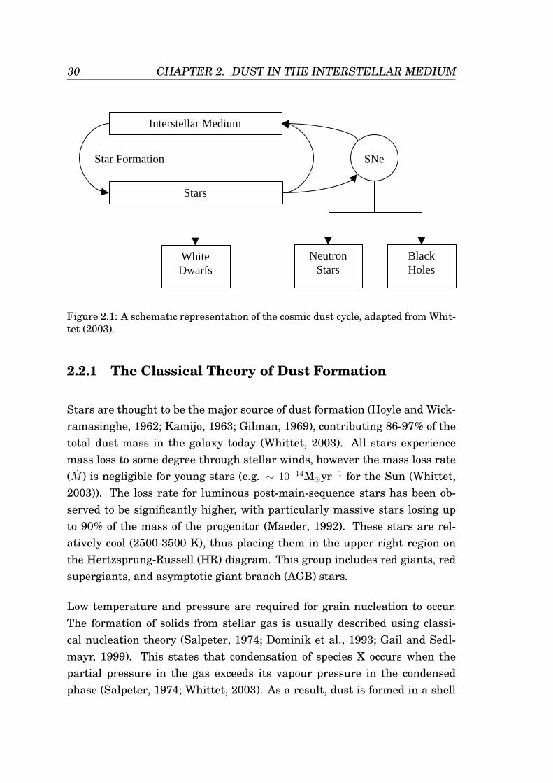
Figure 2.1 is a schematic representation of the cycle through which this ma-terial is processed. Material is thought to be lost from the ISM if it becomescontained within white dwarfs, neutron stars, or black holes, all of whichhave life times greater than the current age of the universe.
The dust cycle is relatively inefficient, with a great deal of material beingtrapped in collapsed stellar remnants. In addition, a great deal of the mate-rial ejected from stars remains hydrogen rich.
2.2 The Origin of Dust in the ISM
Most of the dust in the ISM is thought to be formed in the atmospheres ofstars in the latter stages of their evolution. However, recently it has beenproposed that SNe may also be a significant source of dust creation. In thissection we briefly review these two formation mechanisms, and outline thereason why a significant new dust source, in addition to that from stars, isneeded.
30 CHAPTER 2. DUST IN THE INTERSTELLAR MEDIUM
Interstellar Medium
Stars
White Dwarfs
Neutron Stars
Black Holes
SNeStar Formation
Figure 2.1: A schematic representation of the cosmic dust cycle, adapted from Whit-tet (2003).
2.2.1 The Classical Theory of Dust Formation
Stars are thought to be the major source of dust formation (Hoyle and Wick-ramasinghe, 1962; Kamijo, 1963; Gilman, 1969), contributing 86-97% of thetotal dust mass in the galaxy today (Whittet, 2003). All stars experiencemass loss to some degree through stellar winds, however the mass loss rate(M ) is negligible for young stars (e.g. ∼ 10−14Myr−1 for the Sun (Whittet,2003)). The loss rate for luminous post-main-sequence stars has been ob-served to be significantly higher, with particularly massive stars losing upto 90% of the mass of the progenitor (Maeder, 1992). These stars are rel-atively cool (2500-3500 K), thus placing them in the upper right region onthe Hertzsprung-Russell (HR) diagram. This group includes red giants, redsupergiants, and asymptotic giant branch (AGB) stars.
Low temperature and pressure are required for grain nucleation to occur.The formation of solids from stellar gas is usually described using classi-cal nucleation theory (Salpeter, 1974; Dominik et al., 1993; Gail and Sedl-mayr, 1999). This states that condensation of species X occurs when thepartial pressure in the gas exceeds its vapour pressure in the condensedphase (Salpeter, 1974; Whittet, 2003). As a result, dust is formed in a shell
2.2. THE ORIGIN OF DUST IN THE ISM 31
surrounding a star, rather than in the chromosphere. The inner radius, r1,of this shell is defined by the point at which the temperature falls below thecondensation temperature, Tc, for a particular grain. For a star of radius R?,forming grains with Tc = 1000 K, Bode (1988) estimates r1 ≈ 10R?. The phys-ical conditions (temperature and number density of gas particles, n ∼ 1019
m−3) are optimal at r1, meaning that grain formation occurs quickest at thisradius. The density of material decreases with increased radius, until theedge of the shell is reached, r2, defined as the point at which the tempera-ture and density of the circumstellar material become comparable to that ofthe general ISM (Whittet, 2003).
Data for the mean integrated mass loss rates (Mtot, both gas and dust) in thegalaxy, for various types of star, are contained in Table 2.1. These estimateswere compiled from the literature by Whittet (2003), and derived using,
Mtot = AM?N?, (2.1)
where M? is the mean mass loss rate in Myr−1 for stars of surface numberdensity N?, and A ≈ 1000 kpc2 is the cross-sectional area of the galaxy, in theplane of the disc (Whittet, 2003).
In the case of a low to intermediate mass star (1–8 M), mass loss occursmainly on the asymptotic giant branch, and culminates in the formation ofa planetary nebula (Whittet, 2003). The rates quoted in Table 2.1 for AGBstars are dominated by a small number of stars with particularly high lossrates (Thronson et al., 1987). These stars are inherently more difficult toobserve, as they are embedded in thick circumstellar dust shells, resultingin possible completeness errors. As a result, the estimates quoted here canbe considered lower limits. Taking the figures quoted here, the mass injectedinto the ISM due to all AGB stars is of 1 Myr−1, with an additional 0.3Myr−1 arising from the formation of planetary nebulae (Maciel, 1981). Thisgives a final value of 1.3 Myr−1.
While high mass stars have individually greater mass loss rates, and can beexpected to lose mass throughout their entire lives, their integrated masscontribution to the ISM is small in comparison to that of low to intermediatemass stars (Jura and Kleinmann, 1990). This is because high mass stars
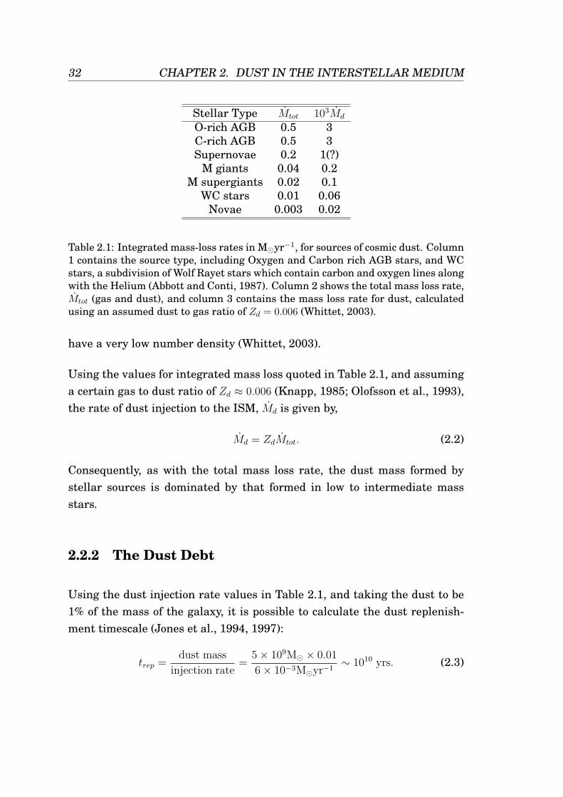
32 CHAPTER 2. DUST IN THE INTERSTELLAR MEDIUM
Stellar Type Mtot 103Md
O-rich AGB 0.5 3C-rich AGB 0.5 3Supernovae 0.2 1(?)
M giants 0.04 0.2M supergiants 0.02 0.1
WC stars 0.01 0.06Novae 0.003 0.02
Table 2.1: Integrated mass-loss rates in Myr−1, for sources of cosmic dust. Column1 contains the source type, including Oxygen and Carbon rich AGB stars, and WCstars, a subdivision of Wolf Rayet stars which contain carbon and oxygen lines alongwith the Helium (Abbott and Conti, 1987). Column 2 shows the total mass loss rate,Mtot (gas and dust), and column 3 contains the mass loss rate for dust, calculatedusing an assumed dust to gas ratio of Zd = 0.006 (Whittet, 2003).
have a very low number density (Whittet, 2003).
Using the values for integrated mass loss quoted in Table 2.1, and assuminga certain gas to dust ratio of Zd ≈ 0.006 (Knapp, 1985; Olofsson et al., 1993),the rate of dust injection to the ISM, Md is given by,
Md = ZdMtot. (2.2)
Consequently, as with the total mass loss rate, the dust mass formed bystellar sources is dominated by that formed in low to intermediate massstars.
2.2.2 The Dust Debt
Using the dust injection rate values in Table 2.1, and taking the dust to be1% of the mass of the galaxy, it is possible to calculate the dust replenish-ment timescale (Jones et al., 1994, 1997):
trep =dust mass
injection rate=
5× 109M × 0.01
6× 10⁻³Myr−1∼ 1010 yrs. (2.3)
2.2. THE ORIGIN OF DUST IN THE ISM 33
The equivalent timescale for dust destruction has been found by Jones et al.(1997), to be tdes ∼ 4− 6× 10⁸ yrs.
These values imply that the dust injection rate is lower than the dust de-struction rate. This would suggest that we should see no significant levelsof dust in the galaxy, which is clearly not the case. Therefore, one of thesevalues must be incorrect. It is unlikely that the dust injection rates for AGBstars has been underestimated by the required factor to account for thisdeficit. It is possible that there is an error in the dust destruction rate, butagain, it is unlikely to be of the magnitude required to explain this differ-ence.
Observations also provide another obstacle to our current theories of dustformation. Recent observations of galaxies (Dunne et al., 2003b; Hugheset al., 1998; Smail et al., 1997) and quasars (Bertoldi et al., 2003; Archibaldet al., 2001) at high redshift have found large amounts of dust (> 108 M), ata point when the universe was only one tenth of its present age (∼1.3 Gyrsold).
It is difficult for this dust to have originated in the stellar winds of evolvedstars, such as those on the AGB. The cycle to produce dust first requiresenrichment of the ISM by rapidly evolving SNe, followed by star formationand evolution. There is insufficient time for such stellar evolution to occurand produce the quantities of dust seen. Therefore, irrespective of any errorsin our estimates of dust formation rate in AGB stars, another significantsource of cosmic dust is needed to explain the observations of dust in theearly universe (Morgan, 2004).
2.2.3 An Alternative Source of Dust
One proposed solution to the dust debt is that the injection rate from pri-mordial SNe is in fact far higher than that stated in Table 2.1. Modelsthat predict significant dust formation (0.2–4 M) in SNe explosions havebeen around for some time (Todini and Ferrara, 2001; Clayton et al., 1999;Woosley and Weaver, 1995; Kozasa et al., 1991); however, it is only recently
34 CHAPTER 2. DUST IN THE INTERSTELLAR MEDIUM
that supporting observational evidence has been available (Dunne et al.,2003a; Morgan et al., 2003).
Infrared data from IRAS and ISO find only very low dust masses, of the order10−4 M, associated with SNe ejecta (Douvion et al., 2001a,b). However, theelemental depletion suggests that the dust mass could be a lot higher (Dweket al., 1992). These values were used to derive the dust injection rates forSNe in Table 2.1. The discrepancy between the predicted dust masses, andthose observed, could be explained if there were a colder (∼15 K) populationof dust particles (Lucy et al., 1991).
Infrared data are biased towards detection of warm dust (∼30 K); far in-frared and submm observations are needed to measure cold dust. Weakobservational evidence for the existence of cold dust in the Cassiopeia Aand Kepler’s supernova remnants (SN remnants), has been found by Dunneet al. (2003a) and Morgan et al. (2003), respectively. These observations wereobtained using the SCUBA instrument on the JCMT. Dunne et al. (2003a)found a dust mass for Cas A of 2–4 M. These results have been contestedhowever by Krause et al. (2004) (see Chapter 7 for further discussion). Ifthese results can be confirmed, then it would mean that SNe would be thedominant known source of dust in the galaxy. The rapid timescales on whichhigh mass stars form, evolve, and ultimately die, means that these sourcesare also capable of explaining the high levels of dust seen in the early uni-verse.
2.3 Star Formation
The mechanisms by which stars form are inextricably linked to the physics ofdust. The properties of dust are fundamental to the collapse processes whichconvert dense cores in molecular clouds to stars, and the stars themselvesgo on to produce more dust. The whole field of star formation research is ex-tremely complex, and will not be dealt with in detail here. Instead I will givea brief overview of the conditions which might lead to core collapse withina molecular cloud, and look at the theoretical collapse solutions, specifically
2.3. STAR FORMATION 35
the Bonnor-Ebert sphere model.
2.3.1 Core Structure and Support
Stars typically form in dense molecular clouds. These clouds can be bestthought of as having a nested hierarchical structure. Within the cloud mediumexists a series of clumps of higher density. These in turn contain a further,more dense, and distinct set of cores (Kirk, 2002). These cores are shieldedby the surrounding medium, allowing them to cool to temperatures of ∼10K (Goldsmith and Langer, 1978).
2.3.2 Core Collapse
The star formation rate in the galaxy is approximately 1 Myr−1 (Knapp,1985). If stars formed via free-fall collapse, then this rate would be anorder of magnitude larger. Instead, cores are supported against collapseby thermal, turbulent and magnetic pressures (Mouschovias, 1976; Mesteland Spitzer, 1956; Curry and Stahler, 2000; Vazquez-Semadeni et al., 2000).These define a critical mass, Mc, that can be supported against gravitationalcollapse.
The maximum critical mass of a magnetised non-rotating pressure-confinedisothermal molecular core, that can be supported against gravitational col-lapse, is approximately the sum of the masses that can be separately sup-ported by the kinetic and magnetic energy of the gas (McKee, 1989; Mouschovias,1976):
Mc = MJ +MΦ. (2.4)
Here, MJ is the Jeans mass, the maximum mass of gas that can be supportedagainst collapse by the kinetic energy of the gas (Jeans, 1920), and MΦ, is itsmagnetic analogue (Mestel and Spitzer, 1956).
A core with M > Mc is termed, supercritical, and is unstable against col-lapse. Conversely a core with M < Mc is termed subcritical, and is stable
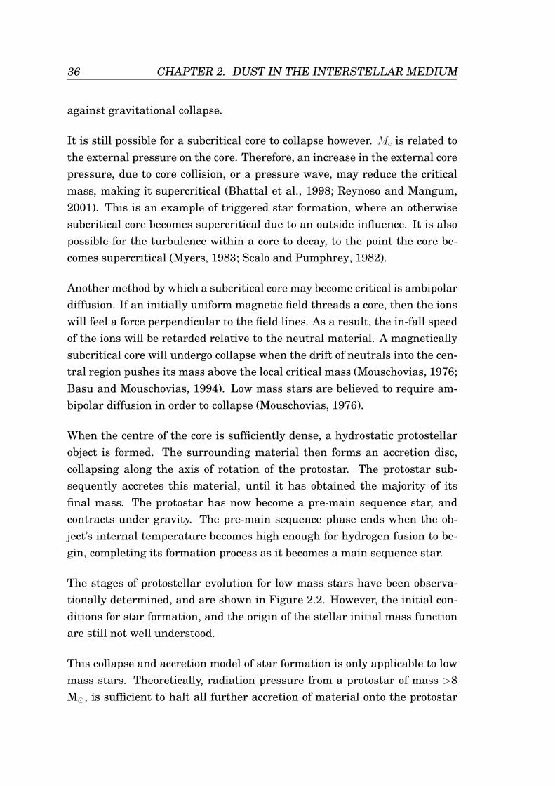
36 CHAPTER 2. DUST IN THE INTERSTELLAR MEDIUM
against gravitational collapse.
It is still possible for a subcritical core to collapse however. Mc is related tothe external pressure on the core. Therefore, an increase in the external corepressure, due to core collision, or a pressure wave, may reduce the criticalmass, making it supercritical (Bhattal et al., 1998; Reynoso and Mangum,2001). This is an example of triggered star formation, where an otherwisesubcritical core becomes supercritical due to an outside influence. It is alsopossible for the turbulence within a core to decay, to the point the core be-comes supercritical (Myers, 1983; Scalo and Pumphrey, 1982).
Another method by which a subcritical core may become critical is ambipolardiffusion. If an initially uniform magnetic field threads a core, then the ionswill feel a force perpendicular to the field lines. As a result, the in-fall speedof the ions will be retarded relative to the neutral material. A magneticallysubcritical core will undergo collapse when the drift of neutrals into the cen-tral region pushes its mass above the local critical mass (Mouschovias, 1976;Basu and Mouschovias, 1994). Low mass stars are believed to require am-bipolar diffusion in order to collapse (Mouschovias, 1976).
When the centre of the core is sufficiently dense, a hydrostatic protostellarobject is formed. The surrounding material then forms an accretion disc,collapsing along the axis of rotation of the protostar. The protostar sub-sequently accretes this material, until it has obtained the majority of itsfinal mass. The protostar has now become a pre-main sequence star, andcontracts under gravity. The pre-main sequence phase ends when the ob-ject’s internal temperature becomes high enough for hydrogen fusion to be-gin, completing its formation process as it becomes a main sequence star.
The stages of protostellar evolution for low mass stars have been observa-tionally determined, and are shown in Figure 2.2. However, the initial con-ditions for star formation, and the origin of the stellar initial mass functionare still not well understood.
This collapse and accretion model of star formation is only applicable to lowmass stars. Theoretically, radiation pressure from a protostar of mass >8M, is sufficient to halt all further accretion of material onto the protostar
2.3. STAR FORMATION 37
Age = 104 yr
Menv > MstarFIR → Submm
Age ~ 105-106 yr
THICK ENVELOPE
IR → Submm
Age ~ 106 - 107 yr
THICK DISKMdisk ~ 0.01M8
V → FIR
Age ~ 107 - 108
yr
THIN DISK?Mdisk ~ 0.003M8
V → IR
Figure 2.2: Schematic showing the evolution of low mass protostars (Andre, 1993).
38 CHAPTER 2. DUST IN THE INTERSTELLAR MEDIUM
(Stahler et al., 2000). This prevents the formation of stars of mass greaterthan this from being formed in this way.
High mass stars appear to form in the centers of dense clusters, leading tothe theory that they might form by the coalescence of several smaller proto-stars (Stahler et al., 2000). Another possible solution has been to vary thestandard model in a qualitative way, such as adjusting the dust properties(Wolfire and Cassinelli, 1987).
High-mass stars are observed to have a very short evolutionary time-scale,or are born almost directly onto the main sequence (Stahler et al., 2000),meaning that observational data regarding their early stages of formation israre. Also, far fewer high mass stars are formed, relative to low mass star,making them even more difficult to find. As a result there is no analogue toFigure 2.2 for high mass star formation.
2.3.3 Collapse Solutions
In the absence of support, a prestellar core will collapse to form a protostar.The form of collapse, for a spherically symmetric core, will be governed bythe variation of density, ρ, with radius, r (Kirk, 2002). A sphere of uniformdensity will undergo free-fall collapse, and every shell of the sphere willreach the centre simultaneously.
The solution for a pressure confined isothermal sphere, in hydrostatic equi-librium, was derived analytically by Chandrasekhar (1939). He found thatfor a sphere of radius Redge, the solution at small radii (r < Rflat) was flat.At larger radii (Rflat < r < Redge) the solution becomes ρ ∝ r−2. The ra-tio of the two radii, ξmax = Rflat/Redge, determines the stability of the coreand the critical value for ξmax, ξcrit, above which a sphere is unstable againstcollapse, is 6.5 (Bonnor, 1956; Ebert, 1955). Spheres parameterised in thisway are termed Bonnor-Ebert spheres (BES). The equation for a BES usesdimentionless forms for density and radius, ξ and ψ, given by
ψ = −ln
(ρ
ρc
), (2.5)
2.4. OBSERVATIONAL PROPERTIES OF DUST 39
ξ =r
as
√4πGρc, (2.6)
where ρ is the local volume density of the gas, ρc is the central density, r isthe radius of a point within the sphere, as is the sound speed, and G is thegravitational constant. These parameters are used to give us the final formof the BES (Bonnor, 1956; Ebert, 1955),
1
ξ2
d
dξ
(ξ2dψ
sξ
)− e−ψ = 0. (2.7)
The limiting case of a sphere of this type, is called a singular isothermalsphere (SIS), and has parameters Rflat = 0, and Redge = ∞ (Shu, 1977). Asphere of this type is fundamentally unstable (Whitworth et al., 1996) andwill will collapse from the inside out, by an expansion wave travelling at thesound speed away from the centre. The analytic simplicity of the SIS modelis attractive; however it suffers from several fundamental flaws: it requiresan infinite central density and an infinite outer radius, and it only allowsfor constant accretion rates. It is not clear that such a sphere could actuallyform (Whitworth et al., 1996).
Conversely, non-uniform accretion rates will occur in a BES of finite and non-zero Rflat and Redge (Foster and Chevalier, 1993). Within Rflat, the constantdensity will result in accretion at almost free-fall speeds. At greater radii,the rate of in-fall decreases to a constant rate, as the outer envelope collapsesinwards. The potential energy released during in-fall must be radiated away,in order keep the sphere isothermal.
2.4 Observational Properties of Dust
2.4.1 The Interaction of Dust with Radiation
A dust grain may interact with radiation by absorption or scattering. Ab-sorption results in the removal of the radiation, and its energy being trans-
40 CHAPTER 2. DUST IN THE INTERSTELLAR MEDIUM
ferred to the absorbing grain, resulting in an increase in dust temperature.The absorbed energy is then re-radiated at a longer wavelength, correspond-ing to the dust grain’s cool temperature. Scattering changes the direction ofpropagation of the radiation, without altering the wavelength. To a distantobserver, it would not be possible to determine which process had occurred.Instead, they would simply see a reduction in the intensity of the source.This removal of radiation from the observers line of sight, due to the sumthe absorption and scattering processes, is known as extinction.
Interstellar and circumstellar dust grains are typically characterised as spher-ical in geometry, with a diameter of ∼ 1 µm. The way in which they coupleto radiation is not however a function of the grain geometry alone. Ratherthan the cross-section for interaction being πa2, as you might expect, wherea is the radius of the grain, theory predicts and experiments have shown,that for small particles it is given by Qπa2. Here, Q is a value which dependson grain properties, such as refractive index and size, and the wavelength ofthe radiation involved (Evans, 1994). In simple terms it can be regarded asan efficiency factor, and is referred to as the Q-factor.
The absorption and scattering efficiencies for a grain with the same incidentradiation can be different, resulting in independent Q-factors for both pro-cesses (Qabs, and Qsca respectively). The Q-factor for extinction is then givenby Qext = Qabs +Qsca.
If a grain is in thermal equilibrium, then the efficiency of emission, Qem
(equivalent to the grain emissivity), is equal to its Qabs. It therefore alsovaries as a function of grain size, and thus wavelength, following the ap-proximate form Qem ∝ λ−β (∝ νβ) (Hildebrand, 1983). The β term can varyfor different grain types, for example, β ≈ 2 for crystalline grains, whereasβ < 2 for more amorphous grains (Draine and Lee, 1984; Whittet, 2003).
2.4.2 Estimating Dust Masses
It is possible to quantify the mass of dust from FIR and submm observations(Hildebrand, 1983). Assuming that the dust grains are spherical, with ra-
2.4. OBSERVATIONAL PROPERTIES OF DUST 41
dius a, volume 4/3πa3, and density ρ, the mass of a cloud of N dust grains, isgiven by
Md =4
3πa3Nρ. (2.8)
The flux density from a cloud of dust grains in thermal equilibrium is givenby Sν = IνΩ, where Iν is the emitted intensity, and Ω is the solid angle. Ifthe background radiation is negligible, then Iν = B(ν, T )(1 − e−τν ), whereτ is the optical depth. In the optically thin limit (τ 1), this reduces toIν = B(ν, T )τν , where τν = πa2NQem. Therefore, the total flux from the cloudat distance D, and temperature T , is
Sν = Nπa2
D2QνB(ν, T ). (2.9)
Rearranging Equations 2.8 and 2.9, in terms of N , the mass of dust becomes
Md =4aρD2Sν
3QemB(ν, T ). (2.10)
The grain dependant parameters are often grouped into a new parameter,known as the dust mass absorption coefficient, κν ,
κν =3Qem
4aρ, (2.11)
giving the final dust mass as,
Md =SνD
2
κνB(ν, T ). (2.12)
Using this it should be possible to make a good estimate of the dust massfor an observation. However, this relies on an accurate value of κ for thedust being known. A wide range of values of κ have been measured andpredicted, from 0.04–0.8 m2 kg−1 at 850 µm (Rowan-Robinson et al., 1986;Sopka et al., 1985; Boulanger et al., 1996; Sodroski et al., 1997; Bianchiet al., 1998; Amure, 2002), depending on the level of processing the dust hasundergone, its environment, and structural type (crystalline or amorphous).Pristine dust can have values of κ an order of magnitude greater than fornormal interstellar dust.
The dust mass absorption coefficient is also proportional to the dust emis-
42 CHAPTER 2. DUST IN THE INTERSTELLAR MEDIUM
sivity index, β, and is a function of Qem. For normal interstellar dust, Jameset al. (2002) derived a value of κ at λ0 = 850 µm of 0.07 m2 kg−1. Using thisas a reference, the value of κ at a given wavelength is given by,
κ = 0.07
(λ0
λ
)β
. (2.13)
The uncertainty in κ is the major source of error in our ability to estimatedust masses from observations.
2.4.3 Cirrus Confusion Noise
The spatial variation in sky background can act as a source of noise, prevent-ing an accurate source flux from being determined. This noise is referred toas confusion noise, and cannot be reduced by performing longer observa-tions. As a result, it represents the fundamental noise limit for an obser-vation. An observation is said to be ‘confusion limited’ if the instrumentalnoise level is less than, or equal to, the confusion noise level.
There are two main contributions to confusion noise at FIR wavelengths.The main component is due to dust emission from irregularly shaped in-terstellar clouds in our own galaxy, the ‘galactic cirrus’ (Low et al., 1984).The second component is from the Extragalactic Background, built up fromthe accumulated light of faint unresolved galaxies along the line of sight(Guiderdoni et al., 1997).
The confusion noise due to cirrus was first characterised by Helou and Beich-man (1990) and Gautier et al. (1992) using IRAS 100 µm data. The secondorder structure function, S(θ), was used,
S(θ) =⟨|B(x− θ)−B(x)|2
⟩x, (2.14)
where B is the sky brightness, x is the location of the source, and θ is theseparation between the source, and the reference sky position. The standardreference configuration used by Gautier et al. (1992) bracketed the sourcemeasurement, by two reference measurements, with a Nyquist separation,
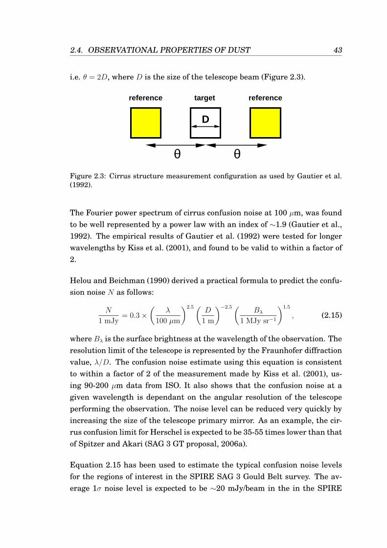
2.4. OBSERVATIONAL PROPERTIES OF DUST 43
i.e. θ = 2D, where D is the size of the telescope beam (Figure 2.3).1162 Cs. Kiss et al.: Sky confusion noise in the far-infrared
reference
θ θ
reference
D
target
Fig. 1. Measurement configuration to compute the structurenoise. Gautier et al. (1992) and Helou & Beichman (1990)derived their results for the resolution limit θmin = 2D. InSect. 3.3 we also consider the cases of θ = k·D, k = 2... 7.
or fractal structure), the only important factor is the θ/Dratio. For their study of the IRAS 100 µm maps Gautieret al. (1992) defined a standard measurement configura-tion where the on-source position is bracketed by two off-source positions separated by ±θ (Fig. 1) and the ratio isfixed to the resolution (Nyquist) limit θ = θmin = 2D.
Gautier et al. (1992) pointed out that the Fourierpower spectra of the IRAS 100 µm scans were generallywell represented by a power law, and that the structurenoise can be linked to the parameters of the power spectraby the following relation:
N ∝(d
d0
)1−α2× P
12
0 (3)
where d−1 is the spatial frequency, d−10 is a reference spa-
tial frequency, P0 is the Fourier power at d−10 , and α is the
spectral index of the Fourier power spectrum. It was alsofound that most scans can be described by the empiricalrelationships α ≈ 3 and P0 ∝ 〈B〉3.
Based on the IRAS results Helou & Beichman (1990)(H&B) proposed a practical formula to predict the cirrusconfusion noise, assuming that the empirical relationshipsof Gautier et al. (1992) are valid at other wavelengths, too.They also took into account that at the resolution limitof the telescope d/d0 can be expressed by the resolutionparameter of Fraunhofer diffraction, λ/Dt, where λ is thewavelength of the measurement and Dt is the diameterof the telescope primary mirror. Under these terms theyexpressed the cirrus confusion noise as:
N H&B
1 mJy= 0.3×
(λ
100 µm
)2.5(Dt
1 m
)−2.5( 〈Bλ〉1 MJy sr−1
)1.5· (4)
Here Bλ is the surface brightness at the wavelength of theobservation. The formula shows that the confusion noisedepends on the wavelength in two separate ways: (1) viathe variation of the surface brightness (spectral energydistribution of the emitting medium) and (2) via the de-pendence of the resolution parameter on λ. This relationwhich is valid for the standard measurement configura-tion as defined in Fig. 1 has been widely used for prepar-ing far-infrared space telescope observations, and appliedeven for other configurations. The first noise analysisof four ISOPHOT maps was performed by Herbstmeieret al. (1998), carrying out the first high spatial resolutionstudy of the galactic cirrus at λ > 100 µm. They proved
that the ISOPHOT sensitivity at far-infrared wavelengthsis limited by sky confusion noise rather than by instru-mental uncertainties.
The confusion noise caused by the CFIRB has dif-ferent properties from the cirrus confusion noise. It canbe represented by a Poissonian spatial distribution, there-fore the confusion noise value is independent of the sep-aration between the target and the reference positions.Ackermann et al. (1992) investigated the sensitivity lim-its, including the effect of the CFIRB, for ISOPHOT andpredicted that the long wavelength observations would belimited by galaxy confusion in the regions of faintest cir-rus. Recently Lagache & Puget (2000), Matsuhara et al.(2000) and Juvela et al. (for an overview see Lemke et al.2000) analysed ISOPHOT maps and separated the cirrusand extragalactic components. They announced the detec-tion of the CFIRB with a fluctuation power in the rangeof 5−12 × 103 Jy2 sr−1 at 170 and 180 µm, close to thepredictions of Guiderdoni et al. (1997). This leads to agalaxy confusion noise limit of 13–22 mJy for ISOPHOTat this wavelength.
For this paper we analysed 175 suitable far-infraredmaps from the ISO Archive. Our goals were (1) to testthe applicability of the Helou & Beichman (1990) formula,especially at λ > 100 µm; (2) to determine the relativecontributions of the galactic cirrus and the extragalac-tic components in the faintest regions of the sky; (3) toderive an easy-to-use formalism for predicting the totalsky confusion noise for instruments on ISO, SIRTF andHERSCHEL and for various measurement configurations,and (4) to determine the Cosmic Far-Infared BackgroundRadiation via its fluctuations.
2. Observations and data analysis
2.1. Selection of ISOPHOT maps
We selected 175 maps from the ISO Archive (Kessler et al.2000), observed in the 90 to 200 µm wavelength range, cov-ering 40 different sky regions. All maps were obtained withthe ISOPHOT instrument (Lemke et al. 1996) on-boardthe ISO satellite (Kessler et al. 1996), in the PHT22 rasterobserving mode (Laureijs et al. 2000). Our selection crite-ria were that the maps should be larger than 5 × 5 rasterpoints, corresponding to ∼8′×8′ for the C100 (3×3 pixelarray, 46′′ pixel size) and C200 (2×2 pixel array, 92′′ pixelsize) detectors. Some maps were observed with full over-sampling, i.e. the field was redundantly covered withoutgaps between detector pixels. The final map images are acomposite of the individual array images on the differentraster positions. The size of the image pixels is always adetector pixel.
We excluded maps with obvious individual structures(resolved stars, galaxies, planetary nebulae, etc.). Thenumber of selected maps is 94, 4, 65 and 12 using theC1 90, C1 100, C2 170 and C2 200 filters, respectively,and they cover a wide range of surface brightnesses(∼1–100 MJy sr−1). A more detailed description of the
Figure 2.3: Cirrus structure measurement configuration as used by Gautier et al.(1992).
The Fourier power spectrum of cirrus confusion noise at 100 µm, was foundto be well represented by a power law with an index of ∼1.9 (Gautier et al.,1992). The empirical results of Gautier et al. (1992) were tested for longerwavelengths by Kiss et al. (2001), and found to be valid to within a factor of2.
Helou and Beichman (1990) derived a practical formula to predict the confu-sion noise N as follows:
N
1 mJy= 0.3×
(λ
100 µm
)2.5 (D
1 m
)−2.5 (Bλ
1 MJy sr−1
)1.5
, (2.15)
where Bλ is the surface brightness at the wavelength of the observation. Theresolution limit of the telescope is represented by the Fraunhofer diffractionvalue, λ/D. The confusion noise estimate using this equation is consistentto within a factor of 2 of the measurement made by Kiss et al. (2001), us-ing 90-200 µm data from ISO. It also shows that the confusion noise at agiven wavelength is dependant on the angular resolution of the telescopeperforming the observation. The noise level can be reduced very quickly byincreasing the size of the telescope primary mirror. As an example, the cir-rus confusion limit for Herschel is expected to be 35-55 times lower than thatof Spitzer and Akari (SAG 3 GT proposal, 2006a).
Equation 2.15 has been used to estimate the typical confusion noise levelsfor the regions of interest in the SPIRE SAG 3 Gould Belt survey. The av-erage 1σ noise level is expected to be ∼20 mJy/beam in the in the SPIRE
44 CHAPTER 2. DUST IN THE INTERSTELLAR MEDIUM
PSW band. This is representative of a region such as Orion (SAG 3 GT pro-posal, 2006a). The confusion noise will be the limiting source of noise forthis survey.
Cirrus confusion noise should not be confused with extragalactic confusionnoise. Extragalactic confusion is defined in a different way, and is not due toemission from dust in the ISM. See Vaisanen et al. (2001) for more informa-tion on extragalactic confusion.
For more information and a good review of cirrus confusion noise at FIRwavelengths, see Kiss et al. (2001, 2005). These articles are particularlyapplicable to space based observatories, such as Spitzer and Herschel.
2.5 Chapter Summary
This chapter has introduced, and reviewed, a range of processes in whichdust plays a major role in the ISM. It has highlighted the important roleplayed by cosmic dust, from chemical processing, to the formation of stars,as well as the cycle through which dust passes, from birth to destruction.
I have reviewed the classical formation mechanism of dust in the atmo-spheres of evolved (AGB) stars, and compared the overall injection rateswith those required to generate the dust fraction seen in the galaxy today.There is a debt in the overall production rate of dust from stars, meaningthat another source of dust must be found to explain the observed levels.The need for a new mechanism of dust formation is further supported by thedetection of dusty galaxies in the early universe. This dust could not havebeen formed by AGB stars, as they would not have had time to reach thenecessary evolutionary stage. The current evidence for supernovae as themissing source is thus introduced.
The process of star formation, collapse and accretion, was then reviewed.The BES core collapse solution was introduced, and the parameterisationcompared to the SIS solution.

2.5. CHAPTER SUMMARY 45
Finally, the interaction of dust with radiation, the method by which dustmasses are estimated, and the concept of confusion noise are introduced.
Further discussion and new results pertaining to the question of dust forma-tion in supernovae will be presented in Chapter 7, and the effect of confusionnoise on SPIRE observations will be addressed in Chapter 8.

46 CHAPTER 2. DUST IN THE INTERSTELLAR MEDIUM
Chapter 3
SPIRE
SPIRE (the Spectral and Photometric Imaging Receiver) is a dual instru-ment comprising a three-band imaging photometer (Figure 3.1(a)) and animaging Fourier transform spectrometer (FTS, Figure 3.2(a)), spanning awavelength range of ∼200–700 µm. The main scientific objectives for SPIREare deep extragalactic and galactic imaging surveys, and spectroscopy ofstar-forming regions in our own, and nearby galaxies.
SPIRE was first proposed in 1998 as an instrument for the Far Infraredand Sub-millimetre Telescope (FIRST), the original name of Herschel. Theconsortium has members from many institutes in seven countries. At thetime of writing, the instrument is undergoing final instrument level testsbefore being delivered to ESA.
In this chapter the basic features of the SPIRE instrument are described,with emphasis on the photometer. This is to set the scene for the descriptionof the SPIRE photometer simulator in Chapter 4. The photometer observingmodes are also reviewed ahead of the optimisation studies in Chapter 6.Finally the SPIRE guaranteed time programmes, currently being plannedby the consortium, are presented.
47
48 CHAPTER 3. SPIRE
3.1 Instrument Overview
SPIRE comprises a cold focal plane unit (FPU), mounted on the Herscheloptical bench (HOB). Modules containing junction field effect transistors(JFETs) and detector pre-amplifier, used for detector read-out, are locatednext to the FPU. The warm electronics are located on the Herschel servicemodule (SVM), and are connected to the FPU by a cold harness.
To review the SPIRE system it is convenient to regard the instrument as aseries of subsystems. In this section an overview of the photometer and FTSwill be presented, followed by a more detailed description of the subsystemscommon to both halves of the instrument.
3.1.1 Photometer
Inside the FPU, the photometer and FTS are arranged back-to-back on eitherside of a central SPIRE optical bench. The photometer side of the FPU isshown in Figure 3.1. It is a three colour instrument with bands centred at250, 360, and 520 µm, with band widths of λ/∆λ ' 3. When the telescopebeam enters the instrument it passes through an optical filter (common filter1, CFIL1, Figure 3.1(b)) into the Level-1 temperature stage (5-K). The beamis then reflected by mirror CM3 before encountering CM4, the beam steeringmirror (BSM). The BSM can be used for spatial modulation of the telescopebeam, allowing the beam to be chopped and jiggled within SPIRE, withoutimpacting on the operation of the Herschel satellite. This unit also containsa photometer calibration source (PCal), located in a cavity behind the centreof the mirror. This acts as a repeatable calibration signal with which to trackdrifts in detector responsivity.
Following this the beam continues to CM5, which produces an intermediatefocal plane at M6, which has two separate elements, the photometer mir-ror 6, PM6, and spectrometer mirror 6, M6. Here the spectrometer field ofview is separated and sent through a hole in the SPIRE optical bench to theFTS side of the instrument by SM6. The photometer beam continues via the
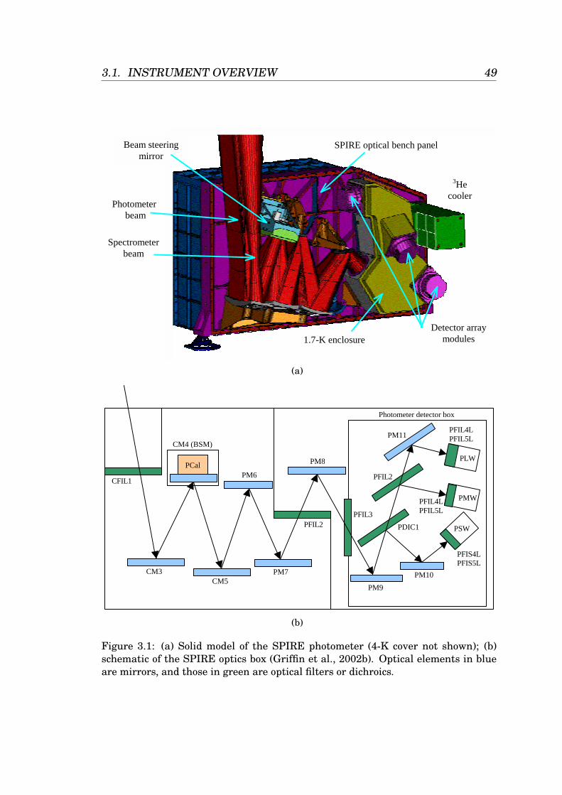
3.1. INSTRUMENT OVERVIEW 49
the 10-K optical bench close to the 4.5-K enclosure, with the JFETs heated internally to their optimum operatingtemperature of ~ 120 K.
The SPIRE warm electronics consist of three units: the Detector Control Unit (DCU), provides bias and signalconditioning for the arrays and cold readout electronics, and reads out the detector signals; the FPU Control Unit(FPU) controls the FPU mechanisms and the 3He cooler, and reads out all FPU thermometers; and the DigitalProcessing Unit (DPU) acts as the interface to the spacecraft for instrument commanding, and telemetry to Earth.
3 IMAGING PHOTOMETER
3.1 OPTICS AND FPU DESIGN
Optics: Figure 1 shows the photometer layout. The 4.5-K optics are mounted directly from the optical bench panel.The 1.7-K enclosure is supported from the panel by stainless steel supports, and contains the detector arrays, thedichroics and fold mirrors. The three array modules are bolted to the outside wall of the 1.7-K box. Within eachbolometer array module, the detector arrays, feedhorns and the final filter are thermally isolated from the 1.7-Kstructure by tensioned Kevlar threads, and are cooled by a thermal strap to the 3He refrigerator (see Section 5). Thephotometer input optics are shared with the spectrometer. The separate spectrometer field of view is directed to theother side of the optical bench panel by a pick-off mirror.
The photometer optical design is illustrated in Fig. 2, and is described in more detail by Dohlen et al.4 It is an all-reflective system except for two dichroics used to direct the three wavelength bands onto different bolometer arrays,and various filters used to define the pass-band and reject out-of-band radiation. The design achieves close todiffraction-limited imaging across the whole 4 x 8 arcminute field of view, which is offset by 11 arcminutes from thecentre of the Herschel telescope's highly curved focal surface. Mirror M3 lies below the focus, and receives the f/8.68Herschel telescope beam and forms an image of the telescope secondary at the flat beam steering mirror, M4. MirrorM5 converts the focal ratio to f/5 and provides an intermediate focus at M6, which re-images the pupil at M4 to a coldstop. M7, M8 and M9 constitute a one-to-one optical relay to bring the M6 focus to the three detector arrays. The
Figure 1: Computer-generated image of the SPIRE photometer layout.
SPIRE optical bench panelBeam steeringmirror
3Hecooler
Detector arraymodules
Photometerbeam
Spectrometerbeam
1.7-K enclosure
(a)
PCal
CM4 (BSM)
CM3 CM5
PM7
PM6
PM8
PM9
PM10
PM11
CFIL1
PFIL2 PFIL3
PDIC1
PFIL2
PFIL4L PFIL5L
PFIL4L PFIL5L
PFIS4L PFIS5L
PSW
PMW
PLW
Photometer detector box
(b)
Figure 3.1: (a) Solid model of the SPIRE photometer (4-K cover not shown); (b)schematic of the SPIRE optics box (Griffin et al., 2002b). Optical elements in blueare mirrors, and those in green are optical filters or dichroics.
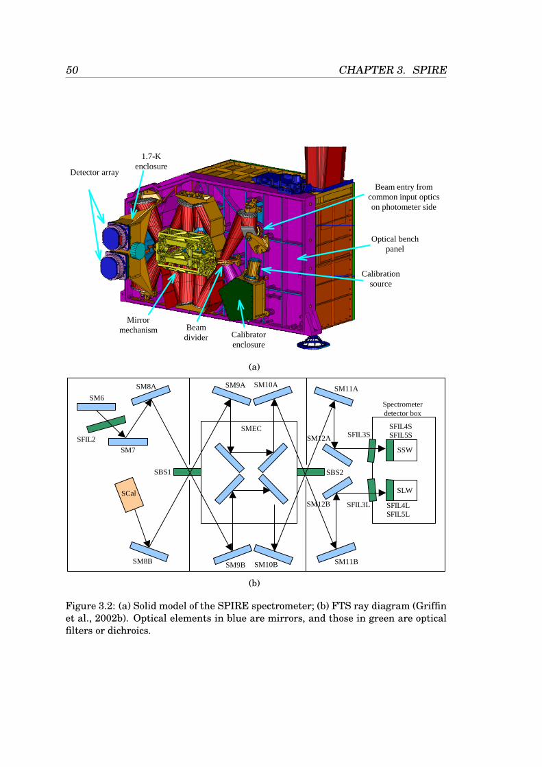
50 CHAPTER 3. SPIRE
4 IMAGING FOURIER TRANSFORM SPECTROMETER
4.1 OPTICS AND FPU DESIGN
The FTS9 uses two broadband, high-efficiency, intensity beam splitters in a Mach-Zehnder configuration rather thanthe traditional polarising beam dividers. This configuration has the advantage that all four ports are separatelyaccessible, as in the classical Martin Puplett (M-P) polarising FTS. But the throughput is a factor of two higher than forthe M-P as none of the incoming radiation is rejected, and there is no sensitivity to the polarisation of the incidentbeam. The performance of the beam dividers and of a bench-top implementation of this design has beendemonstrated10. A thermal source is located at a pupil image in the second input port of the FTS, and provides athermal spectrum that mimics the dilute 80-K black body emission spectrum of the telescope. This allows the largetelescope background to be nulled, thereby reducing the dynamic range requirements for the detector sampling whenthe spectrometer is operated in continuous scan mode. The two FTS detector arrays are placed in the two output ports,with bands of 200-325 µm and 315-670 µm defined by a combination of filters and feedhorn waveguide cutoff. Asingle back-to-back moving roof-top mechanism serves both arms of the interferometer, with a frictionless carriagemechanism using double parallelogram linkage and flex pivots. The scan mirror position readout uses a HeidenhainMoiré fringe sensing system.
Optics: The focal plane layout of the FTS is shown in Fig. 6 and the optical design is illustrated in Fig. 7.
The pick-off mirror (located at the intermediate field image on the photometer side of the optical bench panel) sendsthe spectrometer field of view through a hole in the panel into the FTS side of the instrument. A pupil stop is locatedbetween the pick-off mirror and the input fold mirror. The input relay mirror focuses the beam to an intermediateimage plane located just after the first beam divider, after which the beam is collimated sent to the moving roof-topassembly. The roof-top mirror shifts the beam and sends it towards the camera mirror, which produces an image planejust before the output beam divider. A pupil image is located near the final fold mirror, making this a convenientlocation for the entrance aperture to the 1.7-K enclosure. This pupil moves when the optical path difference changes,
Figure 6: Computer-generated image of the SPIRE FTS layout. The FTS mechanism and the majority of its opticsare mounted on the 4.5-K optical bench panel.
Detector array
1.7-Kenclosure
Optical benchpanel
Beam entry fromcommon input opticson photometer side
Mirrormechanism Beam
divider Calibratorenclosure
Calibrationsource
(a)
SM6
SM7
SM8A SM9A SM10A SM11A
SM12A
SM8B SM9B SM10B SM11B
SM12B
SFIL2
SBS1 SBS2
SFIL3L
SFIL3S SFIL4S SFIL5S
SFIL4L SFIL5L
SSW
SLW
Spectrometer detector box
SMEC
SCal
(b)
Figure 3.2: (a) Solid model of the SPIRE spectrometer; (b) FTS ray diagram (Griffinet al., 2002b). Optical elements in blue are mirrors, and those in green are opticalfilters or dichroics.
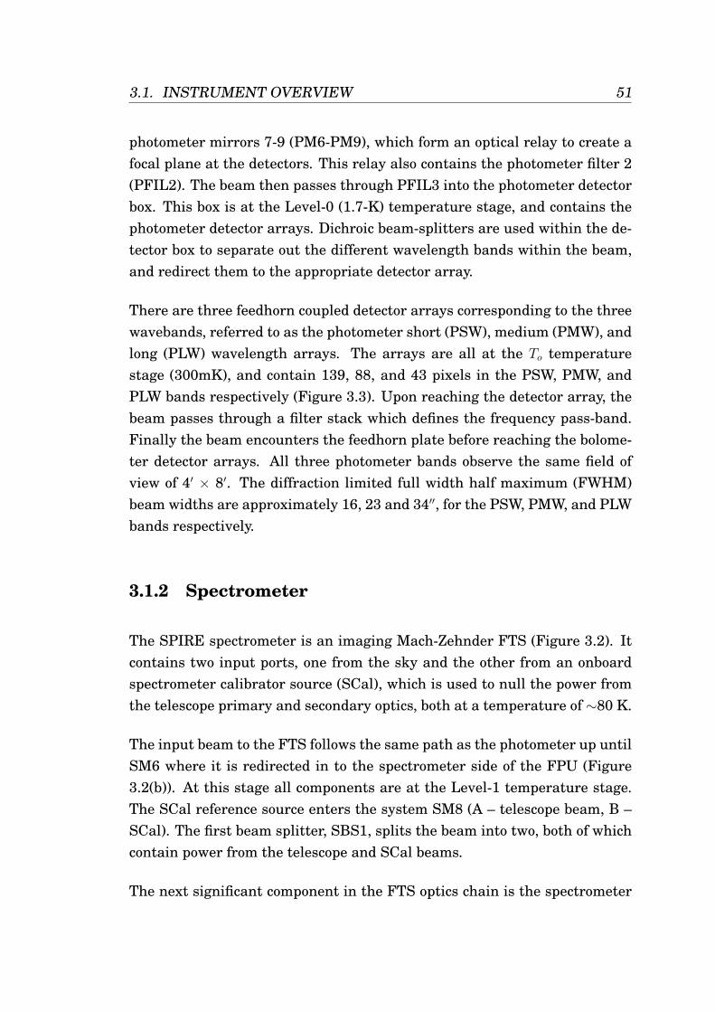
3.1. INSTRUMENT OVERVIEW 51
photometer mirrors 7-9 (PM6-PM9), which form an optical relay to create afocal plane at the detectors. This relay also contains the photometer filter 2(PFIL2). The beam then passes through PFIL3 into the photometer detectorbox. This box is at the Level-0 (1.7-K) temperature stage, and contains thephotometer detector arrays. Dichroic beam-splitters are used within the de-tector box to separate out the different wavelength bands within the beam,and redirect them to the appropriate detector array.
There are three feedhorn coupled detector arrays corresponding to the threewavebands, referred to as the photometer short (PSW), medium (PMW), andlong (PLW) wavelength arrays. The arrays are all at the To temperaturestage (300mK), and contain 139, 88, and 43 pixels in the PSW, PMW, andPLW bands respectively (Figure 3.3). Upon reaching the detector array, thebeam passes through a filter stack which defines the frequency pass-band.Finally the beam encounters the feedhorn plate before reaching the bolome-ter detector arrays. All three photometer bands observe the same field ofview of 4′ × 8′. The diffraction limited full width half maximum (FWHM)beam widths are approximately 16, 23 and 34′′, for the PSW, PMW, and PLWbands respectively.
3.1.2 Spectrometer
The SPIRE spectrometer is an imaging Mach-Zehnder FTS (Figure 3.2). Itcontains two input ports, one from the sky and the other from an onboardspectrometer calibrator source (SCal), which is used to null the power fromthe telescope primary and secondary optics, both at a temperature of ∼80 K.
The input beam to the FTS follows the same path as the photometer up untilSM6 where it is redirected in to the spectrometer side of the FPU (Figure3.2(b)). At this stage all components are at the Level-1 temperature stage.The SCal reference source enters the system SM8 (A – telescope beam, B –SCal). The first beam splitter, SBS1, splits the beam into two, both of whichcontain power from the telescope and SCal beams.
The next significant component in the FTS optics chain is the spectrometer
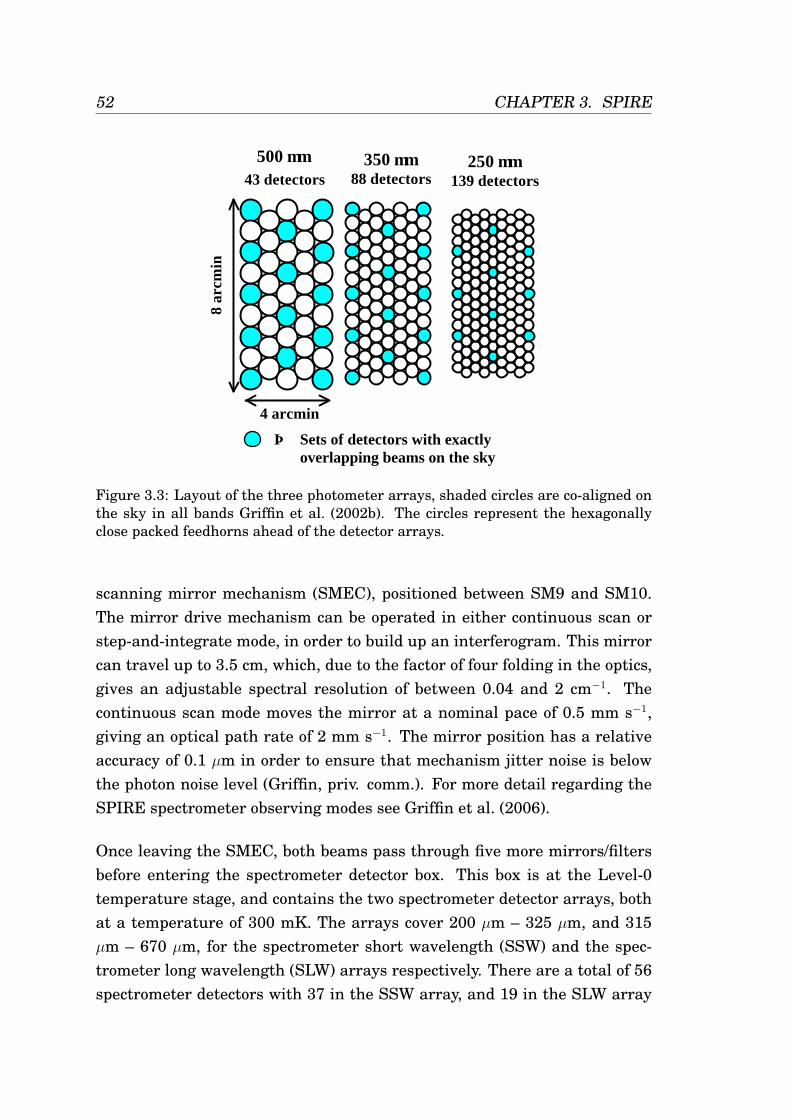
52 CHAPTER 3. SPIRE
8 ar
cmin
500 µm43 detectors
350 µm88 detectors
4 arcmin
⇒ Sets of detectors with exactly overlapping beams on the sky
250 µm139 detectors
Figure 3.3: Layout of the three photometer arrays, shaded circles are co-aligned onthe sky in all bands Griffin et al. (2002b). The circles represent the hexagonallyclose packed feedhorns ahead of the detector arrays.
scanning mirror mechanism (SMEC), positioned between SM9 and SM10.The mirror drive mechanism can be operated in either continuous scan orstep-and-integrate mode, in order to build up an interferogram. This mirrorcan travel up to 3.5 cm, which, due to the factor of four folding in the optics,gives an adjustable spectral resolution of between 0.04 and 2 cm−1. Thecontinuous scan mode moves the mirror at a nominal pace of 0.5 mm s−1,giving an optical path rate of 2 mm s−1. The mirror position has a relativeaccuracy of 0.1 µm in order to ensure that mechanism jitter noise is belowthe photon noise level (Griffin, priv. comm.). For more detail regarding theSPIRE spectrometer observing modes see Griffin et al. (2006).
Once leaving the SMEC, both beams pass through five more mirrors/filtersbefore entering the spectrometer detector box. This box is at the Level-0temperature stage, and contains the two spectrometer detector arrays, bothat a temperature of 300 mK. The arrays cover 200 µm – 325 µm, and 315µm – 670 µm, for the spectrometer short wavelength (SSW) and the spec-trometer long wavelength (SLW) arrays respectively. There are a total of 56spectrometer detectors with 37 in the SSW array, and 19 in the SLW array
3.1. INSTRUMENT OVERVIEW 53
(Figure 3.4). The arrays are operated simultaneously and have a field of viewof 2.6′. These arrays are, like those of the photometer, feedhorn coupled, andcontain band-pass filters mounted directly ahead of the feedhorn plate.
Continuous scan: In this mode the beam steering mechanism is not operating and the scan mirror is moved at constantspeed (nominally 0.5 mm s-1) to modulate the signal. The scan mirror control system uses a digital feedback loop toprovide a constant speed over the scan length, with an accuracy requirement of 1% (goal 0.5%). The radiationfrequencies to be detected are encoded as audio frequencies in the range 3-10 Hz at the detector output. The detectorsare read out asynchronously with the samples time-stamped to match them to the corresponding mirror locations. Themaximum scan length is 3.5 cm, giving an optical path difference of 14 cm taking into account the factor of fourfolding in the FTS optics). To ensure that mechanism jitter noise is well below the photon noise level, a relativeaccuracy of 0.1 µm is required for the mirror position. In order to null the strong telescope background, the FTScalibration source will be on continuously.The mechanism is scanned over the required range with the velocitycontrolled by the drive electronics and the scan is repeated until the desired total integration time has been reached.
Step-and-integrate: In this mode, the scan mirror is placed sequentially at a range of positions to compete a scan. Astep size of 20 µm or less is needed to ensure good over-sampling of the interferogram (corresponding to < 5 µmphysical travel). The scan is repeated until the desired total integration time has been reached. The reference sourcedoes not need to operate because the telescope background is chopped out by the beam steering mechanism.
In principle, Step-and-Integrate provides higher S/N as the calibrator does not need to be operating, reducing photonnoise by a factor of √2. However, Continuous Scan is usually the chosen mode for an FTS as it minimises the effects of1/f noise and reduces the time overhead associated with moving the mirror between positions. It also has the advantagethat the source measurement is referenced against the known internal calibrator rather than an adjacent region of thesky. Step-and-Integrate may be more suited for low resolution observations if the mechanism velocity control does notmeet its stringent stability requirement (dictated by the spectrophotometry mode, in which the spectral information isencoded in the sharp central maximum of the interferogram). Which mode is better in practice will depend on theoverall performance and noise characteristics of the system and the type of observation. Step-and-Integrate may be theoptimum mode for low resolution spectrophotometry and Continuous Scan for higher resolution line spectroscopy.
No on-board processing needs to be done on the FTS data in either mode - all raw interferograms can be telemeteredto the ground within the available 130 kbs data rate.
5 3He COOLER AND 0.3-K THERMAL STRAPS
The same 3He cooler design12 will be used for both the SPIRE and PACS instruments. It uses porous material to adsorbor release a gas when cooled or heated. This type of refrigerator is well-suited to space operation. Gas gap heatswitches are used the control the cooler and there are no moving parts. It can be recycled indefinitely with over 95%duty cycle efficiency and the lifetime is only limited by that of the cold stage from which it is run (in this case, theHerschel cryostat). The evaporation of 3He naturally provides a very stable operating temperature under constant heatload over the entire cycle. The cooler needs no mechanical or vacuum connections and only low-current electricalleads for its operation, making the mechanical and electrical interfaces very simple. For zero-g operation two aspects
Figure 8: Spectrometer detector arrays. The shaded detectors are co-aligned on the sky in the two bands.
SLW array19 detectors
SSW array37 detectors
Figure 3.4: Layout of the two spectrometer arrays, shaded circles are co-aligned onthe sky in both bands, detectors within the black circles signify unvignetted pixels(Griffin et al., 2002b). The circles represent the hexagonally close packed feedhornsahead of the detector arrays.
3.1.3 Optics
The SPIRE optical components include mirrors, dichroic beam-splitters, op-tical filters, and feedhorns, as described above. Due to manufacturing con-straints the hole in Herschel’s 3.5 m diameter primary mirror is slightlylarger than that corresponding to the secondary mirror obscuration. Thisresults in a slightly larger beam sidelobe than would be predicted from thesecondary mirror alone.
All SPIRE detectors are coupled to an array of feedhorns with an aperturesize of 2Fλ, where F is the focal ratio at the detector array, and λ is the cen-tral band wavelength. The photometer feedhorns are single moded, whilethose used in the spectrometer are multi-moded, so that they can accepta wider frequency range. The resulting separation of beams on the skyis 2λ/D, where D is the diameter of the telescope primary mirror. Conse-quently an observation is not fully sampled within the field of view by asingle pointing. Full (Nyquist) sampling can be achieved in any single bandby performing a 16-point jiggle map or by scanning the detector array at an
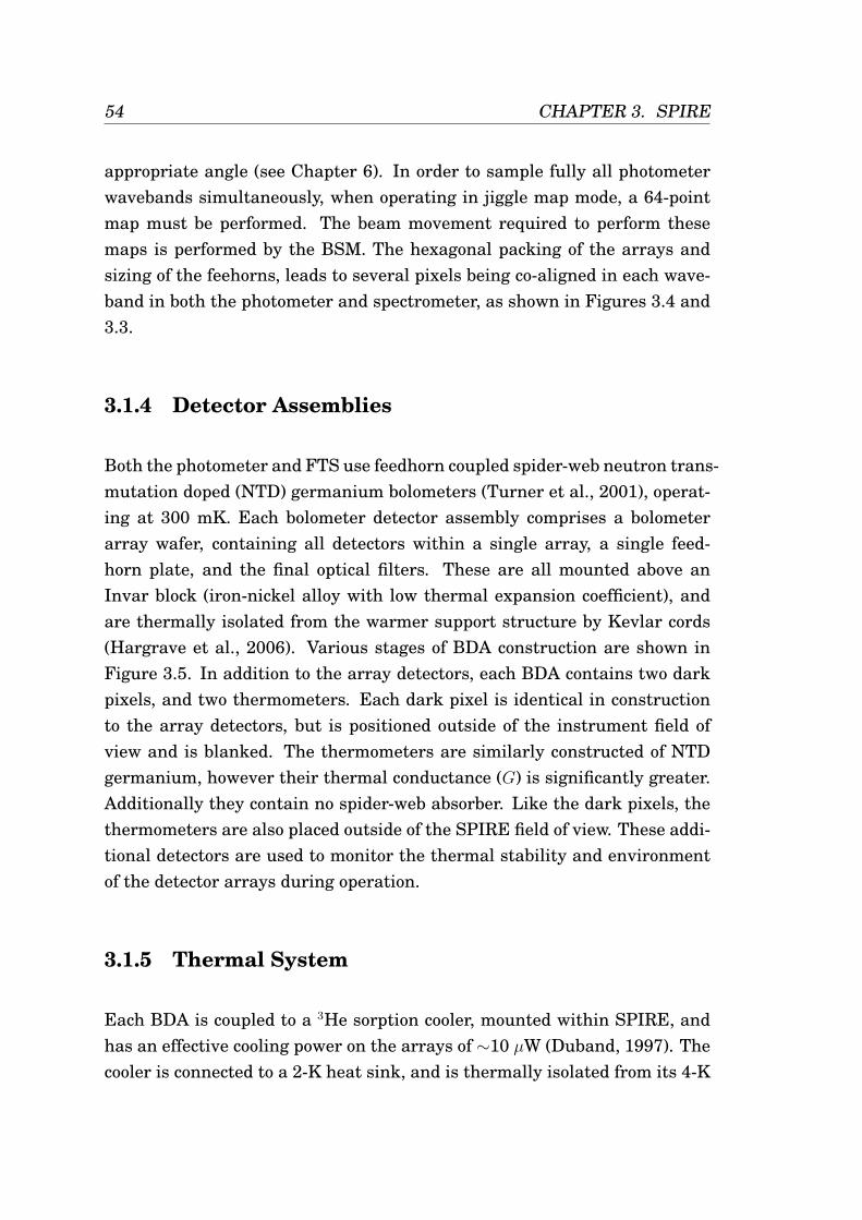
54 CHAPTER 3. SPIRE
appropriate angle (see Chapter 6). In order to sample fully all photometerwavebands simultaneously, when operating in jiggle map mode, a 64-pointmap must be performed. The beam movement required to perform thesemaps is performed by the BSM. The hexagonal packing of the arrays andsizing of the feehorns, leads to several pixels being co-aligned in each wave-band in both the photometer and spectrometer, as shown in Figures 3.4 and3.3.
3.1.4 Detector Assemblies
Both the photometer and FTS use feedhorn coupled spider-web neutron trans-mutation doped (NTD) germanium bolometers (Turner et al., 2001), operat-ing at 300 mK. Each bolometer detector assembly comprises a bolometerarray wafer, containing all detectors within a single array, a single feed-horn plate, and the final optical filters. These are all mounted above anInvar block (iron-nickel alloy with low thermal expansion coefficient), andare thermally isolated from the warmer support structure by Kevlar cords(Hargrave et al., 2006). Various stages of BDA construction are shown inFigure 3.5. In addition to the array detectors, each BDA contains two darkpixels, and two thermometers. Each dark pixel is identical in constructionto the array detectors, but is positioned outside of the instrument field ofview and is blanked. The thermometers are similarly constructed of NTDgermanium, however their thermal conductance (G) is significantly greater.Additionally they contain no spider-web absorber. Like the dark pixels, thethermometers are also placed outside of the SPIRE field of view. These addi-tional detectors are used to monitor the thermal stability and environmentof the detector arrays during operation.
3.1.5 Thermal System
Each BDA is coupled to a 3He sorption cooler, mounted within SPIRE, andhas an effective cooling power on the arrays of ∼10 µW (Duband, 1997). Thecooler is connected to a 2-K heat sink, and is thermally isolated from its 4-K
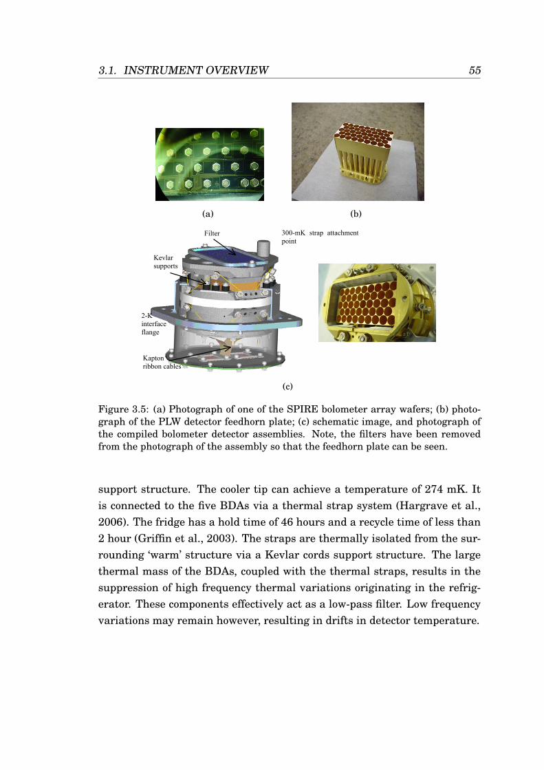
3.1. INSTRUMENT OVERVIEW 55
SPIRE Design Description Document - 2.0
82
this is enormously larger than in the case of optical observations. The accurate subtraction of this thermal background is essential if the much fainter astronomical signals are to be measurable. Furthermore, statistical fluctuation in the arrival rate of these background photons creates a fluctuating noise power which represents a fundamental thermodynamic limitation to the sensitivity. For SPIRE, the associated photon-noise limited NEP, NEPph, is a few x 10-17 W Hz-1/2. In order to achieve photon noise-limited performance, the inherent NEP of the detector system must be comparable to or lower than this. The noise of the bolometer itself is a combination of Johnson noise and phonon noise (due to the quantised flow of thermal energy from the bolometer to the heat sink). The instrument performance models described in §6 contain detailed calculations of the background power levels and sensitivity for SPIRE. In addition, the operating modes require time constants of around 30 ms for the photometer detectors and 16 and 8 ms for the two FTS arrays. With current bolometer technology, these sensitivity and time constant requirements can be met by detectors operating at a temperature of around 0.3 K, cooled by a 3He refrigerator.
4.3.3 SPIRE bolometer design and specifications SPIRE will use arrays of semiconductor bolometers developed at Caltech/JPL. Figure 4-17 illustrates the basic detector design. The absorber is a "spider-web" of metallised silicon nitride. This appears as a filled planar absorber to the submillimetre radiation which has a wavelength much longer than the grid spacing. The spider-web structure has high mechanical strength and a low filling, factor providing low heat capacity and immunity to glitches that can be caused by ionising radiation. The diameter of the spider-web is typically a few times the wavelength to be detected. The thermometer is a small (20 x 100 x 300 µm) crystal of Neutron Transmutation Doped (NTD) germanium. This material is highly suited for use in low temperature bolometers as its thermal behaviour closely approaches that of an ideal thermal device, the material displays very low 1/f noise, and the manufacturing processes are highly repeatable and reliable. A wide range of NTD materials are available to tailor the impedance of the device to the desired range for the chosen operating temperature. Large arrays of bolometers can now be made, as illustrated by the array wafer shown in Figure 4-17.
Figure 4-17 - Left: Photograph of part of a SPIRE P/LW (520-µm) array wafer, showing individual spider-web bolometers and lithographed electrical connections. Right: close-up of an individual bolometer. The dark rectangle is
the TBDxTBD NTD thermometer.
(a)
SPIRE Design Description Document - 2.0
84
Siliconsubstrate
at 300
Conicalfeedhorn
Circularwaveguide
λ/4
2Fλ
Metalisedsilicon
nitride web
NTD Gethermometer
mK Figure 4-19 - Left: feedhorn eedhorn and cavity design. Right: photograph of SPIRE P/LW (500-µm) feedhorn array.
Maximum feedhorn aperture efficiency of 70-80% is achieved for a horn diameter close to 2Fλ (e.g., Griffin, Bock and Gear, 2002), corresponding to a beam spacing on the sky ~ 2λ/D, where D is the telescope diameter. The horn restricts the detector field of view, giving a tapered (near Gaussian) illumination of the telescope primary mirror (with an edge taper of approximately 8 dB in the case of SPIRE). Whilst the horns are close-packed in the focal plane, their beams on the sky do not fully sample the image unless the horn diameter is = 0.5Fλ. Several separate telescope pointings are therefore needed to create a fully-sampled image. For the 2Fλ horns 16 pointings are required in principle, as illustrated in Figure 4-20. In the case of SPIRE, the step size is dictated by the shortest wavelength channel (P/SW - 250 µm) and the number of steps is dictated by the longest wavelength channel (P-LW - 520 µm) so that a 64 point jiggle map is needed to achieve simultaneous full spatial sampling in all photometer bands.
Beam FWHM = λ/D
Beam separation on the sky = 2λ/D
Feedhorns adjacent in the focal plane
Figure 4-20 A 16-point “jiggle pattern” is needed to achieve a fully sampled map with 2Fλ feedhorns (for hexagonal
packing the jiggle pattern is slightly different but 16 steps are still required).
The main advantages of feedhorn arrays are:
(i) maximum efficiency for detection of a point source with known position; (ii) well understood horn properties, allowing good control of the beam and reliable design; (iii) good stray light rejection - the bolometer field of view is restricted to the telescope; (iv) good rejection of EM interference - the horn plus integrating cavity act as a Faraday
enclosure; (v) minimum number of detectors for a given total field size.
(b)
SPIRE Design Description Document - 2.0
85
The main disadvantages are that the observing modes are complicated (jiggling or scanning) and that the efficiency for mapping is a less than the ideal (Griffin, 2000). This means that the full collecting area of the telescope is not used with maximum efficiency. In order to collect the radiation from a point source with good efficiency, the detector through put must be of the order of λ2. The diffraction-limited beamsize of a telescope of diameter D is approximately θ ≈ 1.2λ/D. The corresponding solid angle on the sky is Ωsky = π(θ/2)2. The throughput (the product of area and solid angle, which is conserved in an ideal optical system) is therefore
AtelΩsky ≈ [πD2/4][π(1.2λ/2D)2] ≈ λ2. The SPIRE photometer uses smooth wall, single-mode feedhorns - the circular waveguide section allows propagation of only one mode (TE11). The corresponding throughput (defined as the area-solid angle product) is exactly λ2. The spectrometer uses multi-mode feedhorns that pass both TE and TM modes.
4.3.6 Bolometer array thermal-mechanical design The design of the SPIRE array units (called Bolometer Detector Arrays, BDA's) is illustrated Figure 4-21. Each BDA unit is split into a 2-K and a 300-mK section. The 300-mK section contains the feedhorns, waveguides, bolometer array wafer and the supporting structure. The 2-K detector structure forms the mechanical interface between the 300-mK structure and the photometer or spectrometer 2-K enclosures. The enclosures are connected via thermal straps to the 1.7-K stage of the Herschel cryostat. The heat load from the 2-K structure to the 300-mK structure of the BDA is minimised by suspending the 300-mK section from the 2-K structure with two pre-tensioned 3000-denier Kevlar cords. Kevlar has high mechanical strength in tension and a very low thermal conductivity at this temperature, and forms gives good thermal isolation between the assemblies. The estimated heat load is less than 1.6 µW per array. The high mechanical rigidity of the Kevlar cord yields a high resonant frequency (> 200Hz).
Figure 4-21 - Left: Bolometer Detector Array module design (not incorporating some superficial modifications to the
design that have been recently been introduced). Right: photograph of a prototype P/LW BDA (without the array filter).
Table 4-3 lists the some of the main design and performance parameters for the SPIRE detectors. .
Filter 300-mK strap attachmentpoint
Kevlar supports
2-K interface flange
Kapton ribbon cables
(c)
Figure 3.5: (a) Photograph of one of the SPIRE bolometer array wafers; (b) photo-graph of the PLW detector feedhorn plate; (c) schematic image, and photograph ofthe compiled bolometer detector assemblies. Note, the filters have been removedfrom the photograph of the assembly so that the feedhorn plate can be seen.
support structure. The cooler tip can achieve a temperature of 274 mK. Itis connected to the five BDAs via a thermal strap system (Hargrave et al.,2006). The fridge has a hold time of 46 hours and a recycle time of less than2 hour (Griffin et al., 2003). The straps are thermally isolated from the sur-rounding ‘warm’ structure via a Kevlar cords support structure. The largethermal mass of the BDAs, coupled with the thermal straps, results in thesuppression of high frequency thermal variations originating in the refrig-erator. These components effectively act as a low-pass filter. Low frequencyvariations may remain however, resulting in drifts in detector temperature.
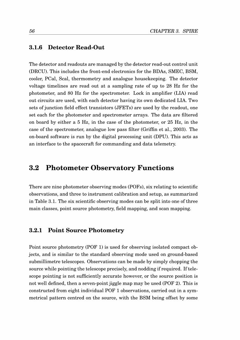
56 CHAPTER 3. SPIRE
3.1.6 Detector Read-Out
The detector and readouts are managed by the detector read-out control unit(DRCU). This includes the front-end electronics for the BDAs, SMEC, BSM,cooler, PCal, Scal, thermometry and analogue housekeeping. The detectorvoltage timelines are read out at a sampling rate of up to 28 Hz for thephotometer, and 80 Hz for the spectrometer. Lock in amplifier (LIA) readout circuits are used, with each detector having its own dedicated LIA. Twosets of junction field effect transistors (JFETs) are used by the readout, oneset each for the photometer and spectrometer arrays. The data are filteredon board by either a 5 Hz, in the case of the photometer, or 25 Hz, in thecase of the spectrometer, analogue low pass filter (Griffin et al., 2003). Theon-board software is run by the digital processing unit (DPU). This acts asan interface to the spacecraft for commanding and data telemetry.
3.2 Photometer Observatory Functions
There are nine photometer observing modes (POFs), six relating to scientificobservations, and three to instrument calibration and setup, as summarizedin Table 3.1. The six scientific observing modes can be split into one of threemain classes, point source photometry, field mapping, and scan mapping.
3.2.1 Point Source Photometry
Point source photometry (POF 1) is used for observing isolated compact ob-jects, and is similar to the standard observing mode used on ground-basedsubmillimetre telescopes. Observations can be made by simply chopping thesource while pointing the telescope precisely, and nodding if required. If tele-scope pointing is not sufficiently accurate however, or the source position isnot well defined, then a seven-point jiggle map may be used (POF 2). This isconstructed from eight individual POF 1 observations, carried out in a sym-metrical pattern centred on the source, with the BSM being offset by some
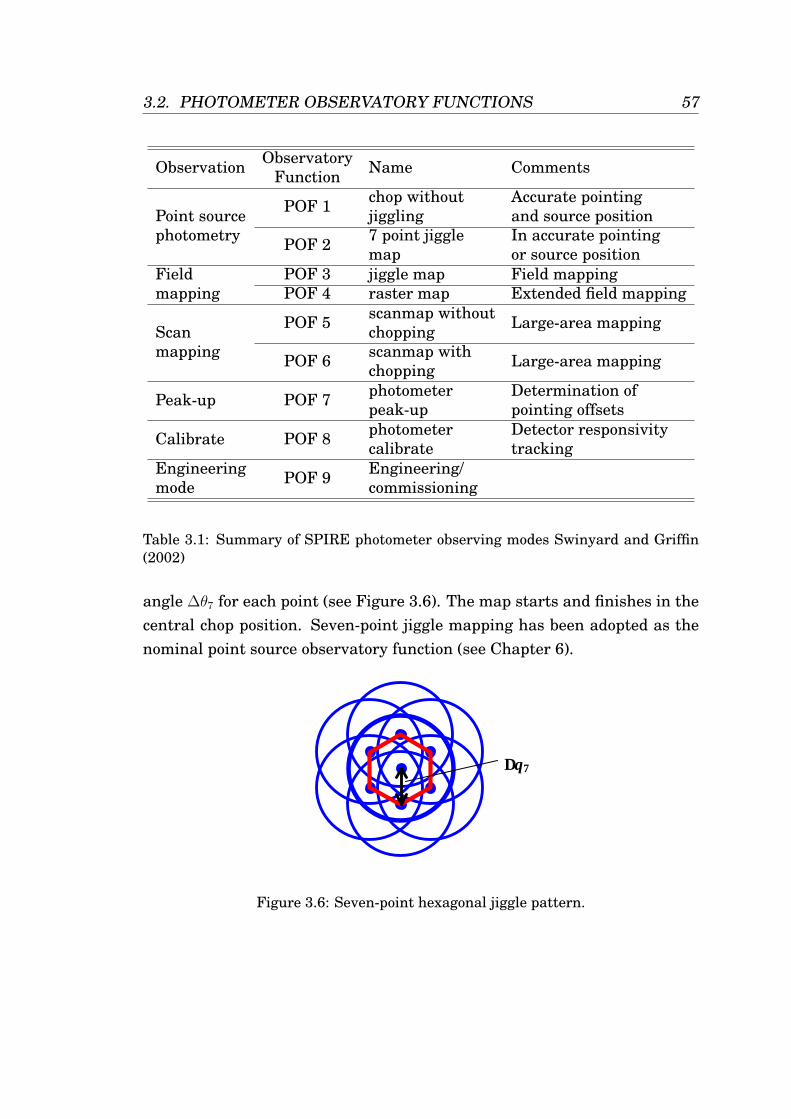
3.2. PHOTOMETER OBSERVATORY FUNCTIONS 57
Observation Observatory Name CommentsFunction
POF 1 chop without Accurate pointingPoint source jiggling and source positionphotometry POF 2 7 point jiggle In accurate pointing
map or source positionField POF 3 jiggle map Field mappingmapping POF 4 raster map Extended field mapping
POF 5 scanmap without Large-area mappingScan choppingmapping POF 6 scanmap with Large-area mappingchopping
Peak-up POF 7 photometer Determination ofpeak-up pointing offsets
Calibrate POF 8 photometer Detector responsivitycalibrate tracking
Engineering POF 9 Engineering/mode commissioning
Table 3.1: Summary of SPIRE photometer observing modes Swinyard and Griffin(2002)
angle ∆θ7 for each point (see Figure 3.6). The map starts and finishes in thecentral chop position. Seven-point jiggle mapping has been adopted as thenominal point source observatory function (see Chapter 6).
Ref: SPIRE-RAL-DOC-000320
Issue: 3.3 Date: June 24 2005 Page: 24 of 24
Project Document
SPIRE Operating Modes for the SPIRE Instrument
Figure 3.3: Seven-point hexagonal jiggle pattern. The order in which the seven points are visited is TBD. The central position is re-visited at the end to make for eight positions altogether.
3. From such a 7-point map, the total flux of the source can be computed (see RD3)
4. At each position in the seven-point, the equivalent of a POF 1 observation (without nodding) is made.
5. Nodding is optional, with the baseline assumption that it will be necessary.
6. If nodding is being implemented, a complete 7-point is carried out in each nod position before the telescope is nodded to the other position.
7. As for POF 1. Although only the primary sets of detectors are essential for this mode, the other detectors in the arrays will also be sampled, providing a sparsely sample map of the region around the source.
On-board processing and data rate: As POF 1.
Instrument and Spacecraft Functions used and their parameters: See Table 3.5.
Instrument Function: Photometer Chop No. Parameter Range of values Nominal value Comments
1 Chop frequency ( fchop) As for POF 1 As for POF 1 2 Chop direction As for POF 1 As for POF 1 3 Chop throw (∆θchop) As for POF 1 As for POF 1 4 Number of chop cycles per
nod position (Nchop) N/A N/A Not specified in this mode
Instrument Function: Photometer Jiggle 1 Jiggle pattern offset of each of
the six neighbour positions from the centre (∆θ7)
3 – 10 arcsec.
6 arcsec. Eight positions are observed: centre + hexagon + centre again.
2 Number of chop cycles/ jiggle position (Nchop)
Min = 2 Max = TBD
16 Nominal time spent in executing jiggle = 8 x 8 = 64 sec.
3 Number of jiggle patterns /nod position (Njigpat)
1 – TBD 1
Spacecraft Function: Nod 1 Nodding As for POF 1 As for POF 1 2 Dwell time on each nod
position (tdwell) Nominally As for POF 1, but BSM overheads may be slightly different
Nominally As for POF 1, but BSM overheads may be slightly different
3 Nod direction As for POF 1 As for POF 1 4 Nod throw (∆θchop) As for POF 1 As for POF 1 5 Total no. of nod cycles (Nnod) As for POF 1 As for POF 1
Table 3.5: Spacecraft and Instrument Functions for POF 2
∆θ7
Figure 3.6: Seven-point hexagonal jiggle pattern.
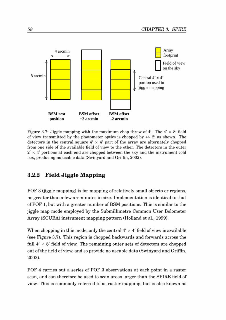
58 CHAPTER 3. SPIRE
BSM rest position
BSM offset +2 arcmin
BSM offset -2 arcmin
Central 4’ x 4’ portion used in jiggle mapping
4 arcmin
8 arcmin
Array footprint
Field of view on the sky
Figure 3.7: Jiggle mapping with the maximum chop throw of 4′. The 4′ × 8′ fieldof view transmitted by the photometer optics is chopped by +/- 2′ as shown. Thedetectors in the central square 4′ × 4′ part of the array are alternately choppedfrom one side of the available field of view to the other. The detectors in the outer2′ × 4′ portions at each end are chopped between the sky and the instrument coldbox, producing no usable data (Swinyard and Griffin, 2002).
3.2.2 Field Jiggle Mapping
POF 3 (jiggle mapping) is for mapping of relatively small objects or regions,no greater than a few arcminutes in size. Implementation is identical to thatof POF 1, but with a greater number of BSM positions. This is similar to thejiggle map mode employed by the Submillimetre Common User BolometerArray (SCUBA) instrument mapping pattern (Holland et al., 1999).
When chopping in this mode, only the central 4′ × 4′ field of view is available(see Figure 3.7). This region is chopped backwards and forwards across thefull 4′ × 8′ field of view. The remaining outer sets of detectors are choppedout of the field of view, and so provide no useable data (Swinyard and Griffin,2002).
POF 4 carries out a series of POF 3 observations at each point in a rasterscan, and can therefore be used to scan areas larger than the SPIRE field ofview. This is commonly referred to as raster mapping, but is also known as
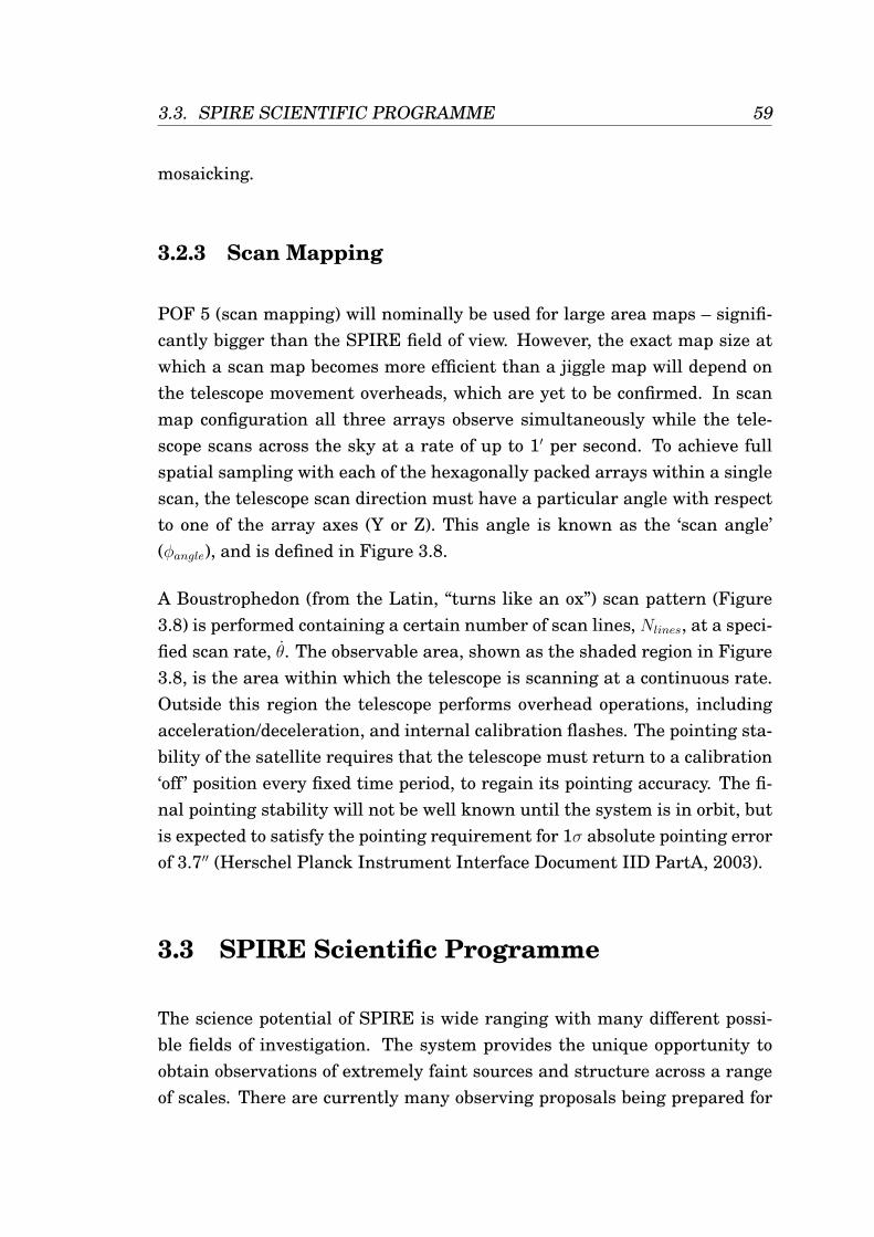
3.3. SPIRE SCIENTIFIC PROGRAMME 59
mosaicking.
3.2.3 Scan Mapping
POF 5 (scan mapping) will nominally be used for large area maps – signifi-cantly bigger than the SPIRE field of view. However, the exact map size atwhich a scan map becomes more efficient than a jiggle map will depend onthe telescope movement overheads, which are yet to be confirmed. In scanmap configuration all three arrays observe simultaneously while the tele-scope scans across the sky at a rate of up to 1′ per second. To achieve fullspatial sampling with each of the hexagonally packed arrays within a singlescan, the telescope scan direction must have a particular angle with respectto one of the array axes (Y or Z). This angle is known as the ‘scan angle’(φangle), and is defined in Figure 3.8.
A Boustrophedon (from the Latin, “turns like an ox”) scan pattern (Figure3.8) is performed containing a certain number of scan lines, Nlines, at a speci-fied scan rate, θ. The observable area, shown as the shaded region in Figure3.8, is the area within which the telescope is scanning at a continuous rate.Outside this region the telescope performs overhead operations, includingacceleration/deceleration, and internal calibration flashes. The pointing sta-bility of the satellite requires that the telescope must return to a calibration‘off ’ position every fixed time period, to regain its pointing accuracy. The fi-nal pointing stability will not be well known until the system is in orbit, butis expected to satisfy the pointing requirement for 1σ absolute pointing errorof 3.7′′ (Herschel Planck Instrument Interface Document IID PartA, 2003).
3.3 SPIRE Scientific Programme
The science potential of SPIRE is wide ranging with many different possi-ble fields of investigation. The system provides the unique opportunity toobtain observations of extremely faint sources and structure across a rangeof scales. There are currently many observing proposals being prepared for
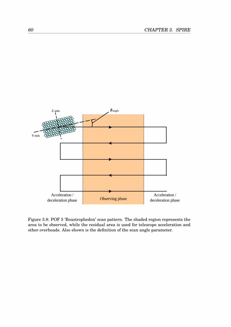
60 CHAPTER 3. SPIRE
Observing phase Acceleration /
deceleration phase Acceleration /
deceleration phase
φangle Z-axis
Y-axis
Figure 3.8: POF 5 ‘Boustrophedon’ scan pattern. The shaded region represents thearea to be observed, while the residual area is used for telescope acceleration andother overheads. Also shown is the definition of the scan angle parameter.
3.3. SPIRE SCIENTIFIC PROGRAMME 61
SPIRE, including those of the SPIRE consortium. The SPIRE consortium ismade up of many instrument scientists and astronomers. In return for thetime spent in development of the system, the consortium receive a guaran-teed 10% of the Herschel mission observing time. This time has been dividedbetween six specialist astronomy groups (SAGs), each focusing on a differentarea of scientific investigation.
The focus of SAG 1 is the observation of high redshift galaxies. This pro-gramme is split into two main sections, the ‘Clusters’ survey, and the ‘Wed-ding Cake’ survey. The first aims to image 15 rich clusters of galaxies, fromz = 0.2 to > 1, to probe the ultimate depth of SPIRE surveys, exploit gravita-tional lensing to detect galaxies below the confusion limit, study the evolvingmember galaxies, and detect the Sunyav ZelDovich (SZ) effect as an incre-ment to the cosmic microwave background signal, and reduce systematiceffects from SZ foregrounds (SAG 1 GT proposal, 2004).
The much larger ‘Wedding Cake’ survey aims to perform a set of blank fieldextra-galactic surveys with SPIRE and PACS. The goals for this programmeinclude (a) to measure the bolometric luminosity density of the Universe athigh redshift (z ≥ 1) - via number count and luminosity function analysis (b)relate the star formation activity at high redshifts to the masses of halos inwhich it is occurring - via clustering (c) to provide the best constraints on thestatistics of the high redshift galaxies comprising the peak of the FIR/submmbackground. The survey will also provide a wide variety of other possiblescience topics which can be addressed since they will provide good samplesof rare (luminous or very high redshift) galaxies (SAG 1 GT proposal, 2005).
The second SAG will concentrate on observations of local galaxies. Thesewill be used to bridge the gap between the local universe and primordialgalaxies. The proposals put forward by SAG 2 aim to investigate the forma-tion of galaxies, the rapid increase in the dust opacity and luminosity of highredshift luminous galaxies, and their subsequent evolution. Observations ofdistant galaxies in the FIR/submm will rely on the spectral energy distribu-tion (SED) to draw conclusions on the processes at work in the distant targetobjects. This SED is almost entirely due to dust emission, and its shape canbe altered by a variety of processes. SAG 2 plans to study two of these ef-
62 CHAPTER 3. SPIRE
fects: (1) the star formation activity of the galaxy, which affects the balancebetween warm and cold dust components, with high star formation activityshifting the SED peak toward shorter wavelengths, and possibly modifyingand destroying the dust, and (2) the metallicity, that drives both the totalabundance of dust in the interstellar medium, and the dust composition, im-pacting in turn the heating and cooling properties. Observations of dwarfgalaxies will be made as their typical star formation activity ranges over 2orders of magnitude, with many of them containing super star clusters. Alsotheir metallicity properties span a large range in the local universe, froma nearly solar value to the lowest levels known in galaxies such as IZw18(1/50 solar metallicity) (SAG 2 GT proposal, 2005b). Both photometric andspectroscopic follow up observations are planned.
Using Herschel’s sensitivity to dust in galaxies, SAG 2 also plan to perform asurvey of 320 nearby galaxies. Goals for this survey include establishing theimportance of dust in galaxies as a source of obscuration in the distant uni-verse, and to study the relationships between star formation and all othercomponents of the interstellar medium, and how they vary with star forma-tion rate. The intergalactic dust cycle will be investigated using observationsof dusty halos, dusty superwinds, and tidally stripped dust around galaxies.The local luminosity and dust mass functions will also be measured, alongwith a further range of objectives (SAG 2 GT proposal, 2005a).
SAGs 3–6 all focus on targets within our own galaxy. The first of the two SAG3 proposals is a survey of the Gould Belt, a ring of nearby star formation re-gions tilted with respect to the galactic plane. It is an extensive imagingsurvey of the densest portion of these star forming complexes with SPIRE at250-500 µm and PACS 110-170 µm, down to a 5σ column-density sensitivityof NH2 = 1021 cm−2 (visual extinction of AV ∼ 1). The nominal sensitivity ofthe survey is well matched to the expected cirrus confusion limit and is suchthat it should be possible to detect dust emission/structure throughout themaps. The target clouds span a range of physical and environmental condi-tions from ‘active’, cluster-forming complexes, to ‘quiescent’ regions with lit-tle or no star formation activity. With ∼20 prestellar condensations expectedper 0.15 dex mass bin between 0.01M and 5M, the predicted numbersof objects are both adequate and necessary to derive an accurate prestel-
3.3. SPIRE SCIENTIFIC PROGRAMME 63
lar core mass function (CMF) from the substellar to the intermediate-massregime. The determination of the CMF is one of the main goals of this sur-vey. The large spatial dynamic range of the proposed SPIRE/PACS surveywill provide a unique view of the formation of dense cores and protoclus-ters within molecular cloud complexes, by probing the link between densecirrus-like structures and compact self-gravitating condensations. The mainscience goal is to elucidate the initial conditions and physical mechanismsresponsible for the formation of prestellar condensations out of the diffuseinterstellar medium (SAG 3 GT proposal, 2006a).
SAG 3 also plans to perform a second survey covering a 20 deg2 area whichwill encompass all of the high-mass star forming regions at less than 3 kpcfrom the Sun. This survey will use accurate and high resolution PACS andSPIRE observations to separate individual high-mass protostars from theirsurroundings and thus determine the fundamental properties of the precur-sors of OB stars for the first time. The data will also provide an unbiasedcensus of both massive pre-stellar cores and massive Class 0 like protostars,and will trace the large-scale emission of the surrounding clouds. This sur-vey will also yield, for the first time, accurate FIR photometry, and thus goodluminosity/mass estimates for a comprehensive and homogeneous sample ofOB-type young stellar objects at all evolutionary stages (SAG 3 GT proposal,2006b).
The scientific motivation of SAG 4 is to trace the evolution of dust grainsin relation to changes of the physical, dynamical and chemical properties ofthe interstellar medium (ISM). This program will provide an unprecedentedview of the structure of the ISM at FIR/submm wavelengths and will enableinvestigation of the impact of dust grains on the ISM physical and chemi-cal state. SPIRE and PACS photometric and spectroscopic observations willprovide the low brightness sensitivity, and spectral information, necessaryto derive the physical properties of the dust and gas, and so completely char-acterize dust evolution. The sensitivity of SPIRE to large spatial scales isparticularly important for this survey (SAG 4 GT proposal, 2006).
SAG 5 will perform spectroscopic observations of objects in the solar sys-tem using all three Herschel spectrometers. HIFI observations of the gas
64 CHAPTER 3. SPIRE
giant planets, Jupiter, Saturn, Uranus, and Neptune, will dominate the pro-gramme. Of special interest is the measurement of water in these planetsatmospheres, the origin of which is still largely unknown. Measurementsof water and other trace elements on Mars may also provide information onphotochemistry of the atmosphere. Many elements predicted to exist canonly be detected with a very sensitive high resolution instrument such asHIFI. Observations tracing the evolution of water and other molecules fromcomets as they become active when approaching the Sun are also planned.Low resolution spectral maps of comets will also be performed using theSPIRE FTS (SAG 5 GT proposal, 2004).
Finally, SAG 6 will study circumstellar disc evolution and the contributionsof evolved stars and supernovae to the dust content of our Galaxy. Deepimaging of five well known discs (rings) that Herschel can resolve, exploit-ing the excellent surface brightness sensitivity of the instrument and allow-ing us to trace spatial variations of the dust properties, will be performed.This programme also builds on a Spitzer legacy survey currently underwaywhich identifies IR-excess stars from a large sample of stars with close tosolar masses and spanning the whole range of ages. Spitzer provides formost of the IR-excess stars only one photometric point (at 70 µm) of the dustemission. PACS and SPIRE will together provide six photometric points atwavelengths that cover the peak of the dust emission, and will thereforeallow a much better definition physical properties of the discs (SAG 6 GTproposal, 2006a).
The second SAG 6 programme will use Herschel’s unique spectral bandsand spectroscopic capabilities to identify and characterise the extended dif-fuse dust emission from sources such as supernova remnants, asymptotic gi-ant branch (AGB) and post-AGB stars. Both photometric and spectroscopicimaging will be employed using SPIRE and PACS. The planned observationswill search for shells and multiple shells around AGB stars, post-AGB andplanetary nebulae, in order to quantify how much mass is lost at variousstages of their evolution, and to attempt to solve the missing mass problemfor such objects (see Section 2.2).
SAG 6 also plans to acquire observations of selected evolved stars with spe-
3.4. CHAPTER SUMMARY 65
cific dust chemistries, in order to characterise fully for the first time dustemission properties in this spectral region. Lastly the group will acquiremulti-wavelength imaging photometry of several young supernova remnants,in order to measure the masses of recently formed cold dust present withinthem and to address the question: are supernovae a major source of dust ingalaxies such as our own (SAG 6 GT proposal, 2006b)?
Many of the surveys outlined above will, in addition to achieving the specificgoals of the various science teams, provide a wide range of valuable dataover a variety of scientific targets. These data will all be public within oneyear of their observation.
3.4 Chapter Summary
In this chapter I have reviewed the SPIRE instrument hardware, observingmodes, illustrated its scientific capabilities by describing some of the SPIREconsortium’s proposed science programmes.

66 CHAPTER 3. SPIRE
Chapter 4
The SPIRE PhotometerSimulator
This chapter describes the design and operation of the SPIRE PhotometerSimulator (SPS), and outlines the motivation behind its development. Afully detailed description can be found in Appendix A.
4.1 Introduction
Software simulators are becoming a common analysis and diagnostic tool forthe development and performance estimation of many complex physical sys-tems, including astronomical instruments. Depending on the sophisticationand timing of development, a simulator can be used to assess the impactof various design solutions available during instrument development. Thisis particularly useful in instances where it is impossible to test the systemprior to use in its final operating environment, such as in space.
The consequence of various systematic effects, and noise sources which can-not be easily calculated by theory, can also be studied using a simulator. Thiscan allow investigation of the operational system performance over a widerange of parameter space.
67
68 CHAPTER 4. THE SPIRE PHOTOMETER SIMULATOR
For example, the effect of some change in an instrumental noise parameter,such as the 1/f noise knee frequency, can be studied, without the need forfurther hardware testing. The appropriate changes to observing parameters,such as scanning rate, can then be implemented, thus helping to achieveefficient operation of the facility. This is particularly important in the caseof a space mission, as any additional commissioning tests would use valuablein-flight observing time.
Finally, a simulator can provide highly realistic data products, allowing ef-ficient development and evaluation of software tools, capable of storing andprocessing the data in an optimal manner.
At its most basic a simulator requires three things: an accurate input fromwhich to work, a model of the system, and an output of a form equivalentto that of the real system. In the case of the SPIRE photometer simulator,the input takes the form of a model of the astronomical sky. The complexityof this model can vary and depends on the study being carried out. Thesystem model is a representation of the physical system, and can again varysignificantly in complexity, with increased sophistication providing a morefaithful output. The simplest form of SPIRE system model would implementan observing pattern for a single detector, and return a sky value for eachtelescope pointing. Such a model is needed so that the final basic elementcan be derived; an output with a form equivalent to that of the true system,in this case, astronomical power and telescope pointing time-lines.
In the past some software packages referred to as ‘instrument simulators’,have in fact been data simulators (e.g. Oliver and Todd, 2000). The outputfrom these systems would often be a beam convolved input sky with someadditional noise imposed in the map, thus representing what an astronomermight ultimately want. This does not therefore constitute an instrumentsimulator as defined above. Results from this type of simulator can, however,be useful to investigate some basic aspects of system performance, such asthe effect of the beam size, and white noise level, on the output data quality.
The SPS is a more advanced instrument simulator, composed of a set of de-tailed subsystem models. It is a modular system coded in Interactive DataLanguage (IDL), with each module representing a particular subsystem. It
4.1. INTRODUCTION 69
allows investigation of a realistic system which incorporates all of the keysystematics and noise contributions expected in the final instrument, in-cluding the impact of certain observing strategies and methods. It does nothowever produce data which are identical in all respects to that of the realsystem. The SPS is highly representative, but could never incorporate theinevitable, and as yet unknown, noise and error contributions that mightarise in operation. It does however allow us to quantify and characterisethe known or anticipated noise and errors which will ideally dominate thesystem performance.
In summary, the purpose of the SPS is to produce simulated SPIRE photome-ter data (both science and housekeeping) timelines, derived from a realisticphysical model of the instrument which “observes” a simulated astronom-ical sky using any of the allowed photometer observing functions (POFs).The sensitivity results should be compatible with the photometer sensitivitymodel, implemented in MATHCAD (Griffin, 2004), but the instrument simu-lator constitutes a much more sophisticated and versatile tool for evaluatingthe photometer performance. The system will be upgraded and extendedto incorporate improvements made in successive versions of the sensitivitymodel, and the results from instrument level tests. The simulated data canbe analysed using a range of data reduction software and the results com-pared with the input sky.
The primary use of data derived from the SPS are:
i. to characterise the systematic effects of the SPIRE photometer, andtheir impact on data quality;
ii. to optimise the observing modes and derive the nominal parameters;
iii. to aid in the development of data pipeline and analysis software;
iv. to help in the planning and optimisation of SPIRE key observations.
70 CHAPTER 4. THE SPIRE PHOTOMETER SIMULATOR
4.2 Simulator Development Plan
A final version of the SPS will take a long time to produce, and will not becomplete until after launch. I have produced the first version by devising amodular architecture and implementing a form of each module. The mod-ular architecture will allow the simulator to be progressively updated andenhanced in a controlled way. The process of enhancing the simulator willcontinue as new and more detailed system models are devised, and will in-corporate work done by a range of specialists within the consortium. Thisdevelopment is expected to take place throughout instrument building andtesting, and also after launch, to ensure that the simulator can representthe real instrument as faithfully as possible.
A similar code has been developed for the FTS Lindner et al. (2004). Whilethis is beyond the scope of this thesis, it should be stated that a similar mod-ular structure has been implemented in this case, meaning that a number ofthe modules can be shared or straightforwardly adapted as necessary.
4.3 Simulator Architecture
The simulator is made up of modules representing instrument systems orsubsystems, called as required to generate time-line data for key instrumentand system parameters.
A key feature, necessary to enable organised updates, is that the modulesare defined with specific inputs and outputs in such a way that the mannerin which the module operates internally (e.g., in physically representing thesystem or subsystem) can be modified without affecting other modules. Inaddition to the detector science data timelines, the timelines (actual andsampled) for various other parameters can be accessed (e.g., detector arraytemperatures, BSM position, etc.)
Time-line generators are based on a single master clock. All samples andthe start of all mechanism movements are at clock ticks. This clock always
4.3. SIMULATOR ARCHITECTURE 71
runs at a frequency greater than, or equal to, the SPIRE photometer sam-pling frequency. This allows processes acting on time scales shorter than thesampling time scale to be included within the system.
4.3.1 Module Summary
A module represents each operational process or system within the Her-schel/SPIRE observing system. There are currently 13 modules within thesimulator architecture, 10 of which are operational in the current version.The modules are outlined below.
Core: The core module manages and runs all operations specific to operatingthe simulation software, such as calling other modules in the correct order,performing the required number of simulations, and setting the simulationoutput file names. It does not represent any physical part of the Herschel-SPIRE system.
Sky: This module produces a simulation of the area of sky to be observed,with a resolution finer than the SPIRE beam. In most cases the sky is loadedfrom a file; however, for debugging test simulations, a default blank can becreated by this module. One sky must be set for each waveband.
Input: The input module specifies the observation in “astronomer’s terms”,i.e. right ascension and declination. This module is not yet operational inthe current version of the simulator.
Optics: This module represents the main optical properties and parametersof the telescope and the SPIRE photometer (including the filters), and thepositional mapping of the detectors on the sky. If required, the convolutionof the sky with the telescope beam is also performed within this module.
BSM: The BSM module simulates the BSM pointing time-line, i.e. chop andjiggle movements.
Obsfun: The observatory function module specifies the photometer observ-ing mode to be simulated in terms of the appropriate observatory function
72 CHAPTER 4. THE SPIRE PHOTOMETER SIMULATOR
and its parameters. The input parameters are as defined in the observingmodes document (Swinyard and Griffin, 2002). The commanded and actual(i.e. with pointing error) telescope pointing time-lines are also simulatedhere.
Thermal: This module simulates all information on the temperatures of theinstrument and the telescope, and their temporal fluctuations.
Astropower: This module generates a time-line for the power on each de-tector from the astronomical sky, for each observatory mode pointing (tele-scope + BSM).
Background: The background power module generates a time-line for thebackground power incident on each detector, due to all of the contributionsfrom thermal fluctuations.
Detectors: This module produces an output voltage time-line for each detec-tor channel based on inputs from the Astropower and Background modules.A thermal model of the detector is used to generate the correct voltage out-put, and estimate the detector noise. A voltage time-line with the correctnoise properties is also output by this module.
Sampling: The sampling module produces a data time-line filtered by theon-board 5-Hz low pass filter and sampled at the appropriate sampling rate.
HK: The house keeping module outputs time-lines for all instrument tem-peratures. This module is not yet implemented in the current version of thesimulator.
PCal: Finally, the photometer calibrator module produces a timeline of thepower incident on each detector from PCal. This module is not yet opera-tional in the current version of the simulator.
4.4. SPS OPERATION 73
4.4 SPS Operation
The SPS runs via a four-phase process. These processes are as follows:
1. Input – parameter input phase, set up of module structures with inputparameters;
2. Initialisation – module initialisation and run of non-time step (static)operation modules;
3. Time step – time stepped operation phase, each module is called onceeach time step;
4. After run – finalisation and post processing of time step time lines, e.g.sampling.
There is the opportunity for each module to run at each stage dependingon its functionality and operating processes. In most cases a module willperform its primary task in only one operation phase.
Each phase is initiated via the central SPS core program file, SPS.pro.
4.4.1 SPS Control
The core control program progresses through each operation phase in turn,as shown in Figure 4.1. Correspondingly there are four calling sequences foreach module, one for each phase. These sequences call a routine specific tothe current phase of operation for a specific module and pass the requiredparameters. The parameters within the structures are then converted, asrequired, into a usable form, before being passed to the central module code.This code contains the modelled subsystem which, once complete, outputsits required data back to the module phase routine. These data are thenappended to the module’s own parameter structure, and the associated mod-ule label parameters updated, before returning to the control program. Themodule phase routines (file names) contain the suffix input, init, step, orafterrun, depending on the specific phase of operation they refer to.
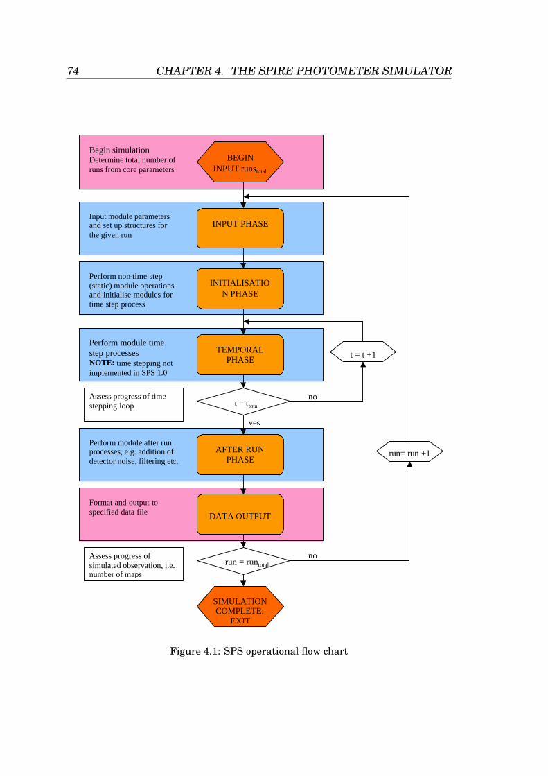
74 CHAPTER 4. THE SPIRE PHOTOMETER SIMULATOR
run= run +1
BEGIN INPUT runstotal
INPUT PHASE
INITIALISATION PHASE
TEMPORAL PHASE
t = ttotal
no
AFTER RUN PHASE
yes
DATA OUTPUT
run = runtotal
no
SIMULATION COMPLETE:
EXIT
Begin simulation Determine total number of runs from core parameters
Input module parameters and set up structures for the given run
Perform non-time step (static) module operations and initialise modules for time step process
Perform module time step processes NOTE: time stepping not implemented in SPS 1.0
Assess progress of time stepping loop
Perform module after run processes, e.g. addition of detector noise, filtering etc.
Format and output to specified data file
Assess progress of simulated observation, i.e. number of maps
t = t +1
Figure 4.1: SPS operational flow chart
4.4. SPS OPERATION 75
4.4.2 Master Clock
All timeline parameters must be simulated with a time step sufficientlysmall compared to the data sampling time. The nominal simulator time-step for the photometer detectors is one-third the instrument-sampling rate.Time line output parameters created by modules in the initialisation phasemust be created with a sampling time step equivalent to that performed inthe time step phase.
The maximum telescope scan rate is 60′′/s, so the time to cross 1/10th of abeam at 250 µm (approx 2′′, the nominal input map resolution) is 1/30 s. Toensure that all quantities are sufficiently finely sampled, a master clock stepof no more than ∼30 ms is therefore required. A nominal step size of 12 msis preferred for a system sampling rate of 28 Hz. The total number of masterclock ticks in an observation timeline is given by
nticks =ttot
∆tclk(4.1)
4.4.3 Parameters
There exists an independent ‘structure’ each module. All input and out-put variable parameters within the simulator are stored within one of thesestructures, determined by their ‘parent’ module (module with which the pa-rameter is associated). In addition to these module structures there is alsoa module ‘label’ parameter. This parameter is a string array containing ashort piece of information describing the parameters, in order, within eachstructure. Each time a new parameter is added to a module structure, themodule label is also updated. All new parameters and labels are appendedto the end of the current structure/label list.
Modules incorporate both input and output parameters, which are subdi-vided in to the categories as set out below.
1. Input parameters: these are parameters to be supplied to a module inorder for it to operate. The inputs required at each phase of operation
76 CHAPTER 4. THE SPIRE PHOTOMETER SIMULATOR
may be different depending on the module functionality and purpose:
(a) User inputs – input parameters supplied by the user via the pa-rameter files;
(b) Module inputs – input parameters derived from hard coded datawithin the simulator;
(c) System inputs – input parameters to one module, created by aprevious module operation, within the same simulation.
2. Output parameters: these are parameters generated by module pro-cesses. Each module may output different parameters at each phaseof operation. Subsequent modules may use these outputs as input pa-rameters:
(a) System outputs – output parameters which describe fixed (non-time varying) parameters within the observing system, e.g. opticaltransmission;
(b) Timeline outputs – derived system parameter time lines, e.g. as-tronomical power time line;
(c) Map outputs – output maps representing the sky as seen by theobserving system, e.g. convolved sky maps.
Timeline output parameters can be of three kinds:
1. Command timelines: these are time-lines of commanded parameters,such as telescope or BSM position, which are available without errorfor the data analysis;
2. Hidden timelines: these are time-lines which are produced by the mod-ule corresponding to quantities which cannot in reality be directly avail-able to the instrument user - an example is the actual telescope point-ing timeline as opposed to the commanded timeline: the former isequivalent to the latter but with added noise, the details of which willnever be available from the data stream;
3. Measured timelines: these are timelines of measured (sampled) scienceor housekeeping data.
4.5. COORDINATE SYSTEMS 77
These subcategories of timeline parameters are not explicitly separated withinthe simulator operation. These are important only to those users who wishto use only those parameters available from the physical system. The classof each time line is specified in the accompanying module documentation.
4.4.4 Data Volume
Each time line is a vector of i = 1 - nticks parameter values, corresponding totimes from 0 to ttot in steps of ∆tclk (the clock interval). There are approxi-mately 300 detectors in total, each with four output timelines: astronomicalpower, noiseless detector voltage, noisy detector voltage, and sampled de-tector voltage. Therefore the total number of output timelines is ∼1200,meaning that the total number of data points needed for a full one-hour sim-ulation is in the order of 3× 10⁸, based on the baseline master clock intervalbeing 12 ms, producing 300,000 points per timeline for a 1-hr observation. Inaddition to these there will also be other memory requirements from otherlarge arrays, e.g. input sky maps.
4.5 Coordinate Systems
The spacecraft and array coordinate system is as shown in Figure 4.2. Thetelescope boresight is the X direction, with the nominal Sun direction alongthe Z axis. The detector arrays are in the Y-Z plane. The three arrays overlapon the sky, ideally with no misalignment. In practice there will be somemisalignment: the centre of the PSW array is defined to be the (0,0) position.
The chopping/nodding direction is along the Y-axis. For scanning observa-tions, the telescope scan direction is defined with respect to the Z axis asshown.
Coordinates in the Y-Z plane can be expressed in arcseconds on the sky ormm in the focal plane with angle on the sky related to distance in the focalplane related by the plate scale equation. The telescope boresight position
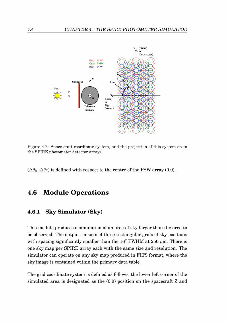
78 CHAPTER 4. THE SPIRE PHOTOMETER SIMULATOR
Y
Z
X
Sun
Sunshield
Telescope primary
y (mm) or ∆θy (arcsec)
φ can
Red: PLW Green: PMW Blue: PSW
Z
z (mm) or ∆θy (arcsec)
Y
Z
Figure 4.2: Space craft coordinate system, and the projection of this system on tothe SPIRE photometer detector arrays.
(∆θy, ∆θz) is defined with respect to the centre of the PSW array (0,0).
4.6 Module Operations
4.6.1 Sky Simulator (Sky)
This module produces a simulation of an area of sky larger than the area tobe observed. The output consists of three rectangular grids of sky positionswith spacing significantly smaller than the 16′′ FWHM at 250 µm. There isone sky map per SPIRE array each with the same size and resolution. Thesimulator can operate on any sky map produced in FITS format, where thesky image is contained within the primary data table.
The grid coordinate system is defined as follows, the lower left corner of thesimulated area is designated as the (0,0) position on the spacecraft Z and
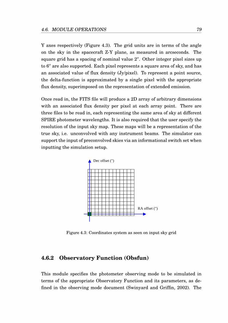
4.6. MODULE OPERATIONS 79
Y axes respectively (Figure 4.3). The grid units are in terms of the angleon the sky in the spacecraft Z-Y plane, as measured in arcseconds. Thesquare grid has a spacing of nominal value 2′′. Other integer pixel sizes upto 6′′ are also supported. Each pixel represents a square area of sky, and hasan associated value of flux density (Jy/pixel). To represent a point source,the delta-function is approximated by a single pixel with the appropriateflux density, superimposed on the representation of extended emission.
Once read in, the FITS file will produce a 2D array of arbitrary dimensionswith an associated flux density per pixel at each array point. There arethree files to be read in, each representing the same area of sky at differentSPIRE photometer wavelengths. It is also required that the user specify theresolution of the input sky map. These maps will be a representation of thetrue sky, i.e. unconvolved with any instrument beams. The simulator cansupport the input of preconvolved skies via an informational switch set wheninputting the simulation setup.
RA offset (")
Dec offset (")
Figure 4.3: Coordinates system as seen on input sky grid
4.6.2 Observatory Function (Obsfun)
This module specifies the photometer observing mode to be simulated interms of the appropriate Observatory Function and its parameters, as de-fined in the observing mode document (Swinyard and Griffin, 2002). The
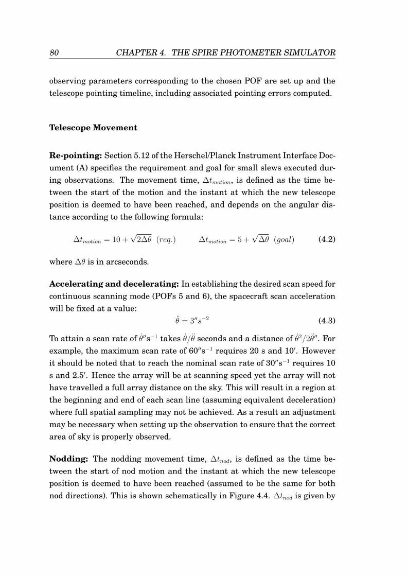
80 CHAPTER 4. THE SPIRE PHOTOMETER SIMULATOR
observing parameters corresponding to the chosen POF are set up and thetelescope pointing timeline, including associated pointing errors computed.
Telescope Movement
Re-pointing: Section 5.12 of the Herschel/Planck Instrument Interface Doc-ument (A) specifies the requirement and goal for small slews executed dur-ing observations. The movement time, ∆tmotion, is defined as the time be-tween the start of the motion and the instant at which the new telescopeposition is deemed to have been reached, and depends on the angular dis-tance according to the following formula:
∆tmotion = 10 +√
2∆θ (req.) ∆tmotion = 5 +√
∆θ (goal) (4.2)
where ∆θ is in arcseconds.
Accelerating and decelerating: In establishing the desired scan speed forcontinuous scanning mode (POFs 5 and 6), the spacecraft scan accelerationwill be fixed at a value:
θ = 3′′s−2 (4.3)
To attain a scan rate of θ′′s−1 takes θ/θ seconds and a distance of θ2/2θ′′. Forexample, the maximum scan rate of 60′′s−1 requires 20 s and 10′. Howeverit should be noted that to reach the nominal scan rate of 30′′s−1 requires 10s and 2.5′. Hence the array will be at scanning speed yet the array will nothave travelled a full array distance on the sky. This will result in a region atthe beginning and end of each scan line (assuming equivalent deceleration)where full spatial sampling may not be achieved. As a result an adjustmentmay be necessary when setting up the observation to ensure that the correctarea of sky is properly observed.
Nodding: The nodding movement time, ∆tnod, is defined as the time be-tween the start of nod motion and the instant at which the new telescopeposition is deemed to have been reached (assumed to be the same for bothnod directions). This is shown schematically in Figure 4.4. ∆tnod is given by
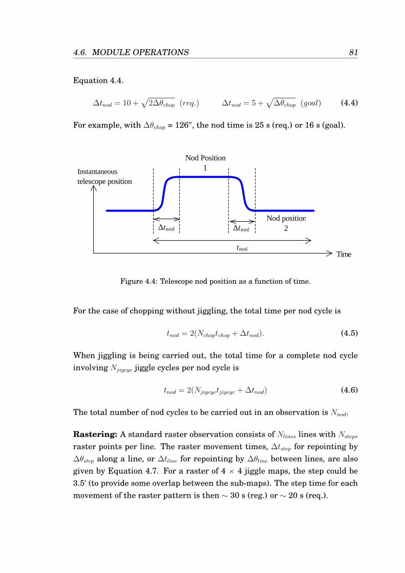
4.6. MODULE OPERATIONS 81
Equation 4.4.
∆tnod = 10 +√
2∆θchop (req.) ∆tnod = 5 +√
∆θchop (goal) (4.4)
For example, with ∆θchop = 126′′, the nod time is 25 s (req.) or 16 s (goal).
Instantaneous telescope position
Time
Nod Position 1
Nod position 2 ∆tnod ∆tnod
tnod
Figure 4.4: Telescope nod position as a function of time.
For the case of chopping without jiggling, the total time per nod cycle is
tnod = 2(Nchoptchop + ∆tnod). (4.5)
When jiggling is being carried out, the total time for a complete nod cycleinvolving Njigcyc jiggle cycles per nod cycle is
tnod = 2(Njigcyctjigcyc + ∆tnod) (4.6)
The total number of nod cycles to be carried out in an observation is Nnod.
Rastering: A standard raster observation consists of Nlines lines with Nsteps
raster points per line. The raster movement times, ∆tstep for repointing by∆θstep along a line, or ∆tline for repointing by ∆θline between lines, are alsogiven by Equation 4.7. For a raster of 4 × 4 jiggle maps, the step could be3.5′ (to provide some overlap between the sub-maps). The step time for eachmovement of the raster pattern is then ∼ 30 s (reg.) or ∼ 20 s (req.).
82 CHAPTER 4. THE SPIRE PHOTOMETER SIMULATOR
The total time spent in moving the telescope between raster positions is
∆trast = (Nstep − 1)∆tstep + (Nlines − 1)∆tline. (4.7)
Scanning: A standard scanning observation consists of Nlines scans, each oflength ∆θscan with spacing ∆θline. A line scan is not deemed to have starteduntil the telescope has attained the required scan speed, θ. The telescopeturn around time at the end of each line is ∆tturn, defined as the time betweenthe end of one line scan and the start of the next. The simulator assumesthat
i. the times needed to accelerate and decelerate the telescope are equal;
ii. the acceleration/deceleration is instantaneous and constant upon be-ginning and ending a scan line;
iii. the telescope turns around using a square pattern, coming to rest ateach corner.
The total turn-around time is then
∆tturn =2θ
θ(4.8)
The total time for an observation is
ttot = Nlines(θ∆θscan + ∆tturn), (4.9)
where we also assume a time ∆tturn/2 is needed both for the first accelerationat the start, and the last deceleration at the end of the observation.
Pointing Error
The pointing errors are defined in the Herschel Planck Instrument InterfaceDocument IID PartA (2003) and shown in Table 4.1
Absolute pointing error: The absolute pointing error (APE) is imple-mented as a random positional offset in both the Z and Y direction upon the
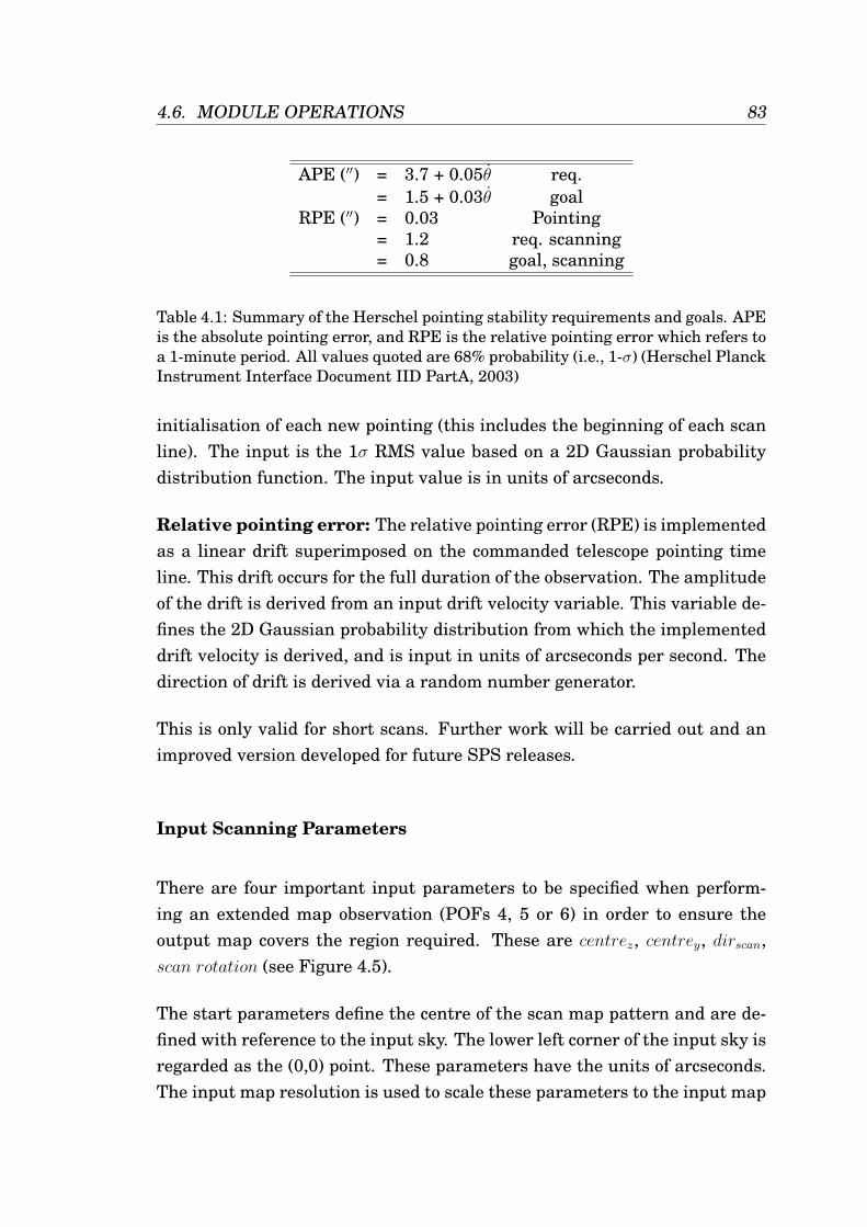
4.6. MODULE OPERATIONS 83
APE (′′) = 3.7 + 0.05θ req.= 1.5 + 0.03θ goal
RPE (′′) = 0.03 Pointing= 1.2 req. scanning= 0.8 goal, scanning
Table 4.1: Summary of the Herschel pointing stability requirements and goals. APEis the absolute pointing error, and RPE is the relative pointing error which refers toa 1-minute period. All values quoted are 68% probability (i.e., 1-σ) (Herschel PlanckInstrument Interface Document IID PartA, 2003)
initialisation of each new pointing (this includes the beginning of each scanline). The input is the 1σ RMS value based on a 2D Gaussian probabilitydistribution function. The input value is in units of arcseconds.
Relative pointing error: The relative pointing error (RPE) is implementedas a linear drift superimposed on the commanded telescope pointing timeline. This drift occurs for the full duration of the observation. The amplitudeof the drift is derived from an input drift velocity variable. This variable de-fines the 2D Gaussian probability distribution from which the implementeddrift velocity is derived, and is input in units of arcseconds per second. Thedirection of drift is derived via a random number generator.
This is only valid for short scans. Further work will be carried out and animproved version developed for future SPS releases.
Input Scanning Parameters
There are four important input parameters to be specified when perform-ing an extended map observation (POFs 4, 5 or 6) in order to ensure theoutput map covers the region required. These are centrez, centrey, dirscan,scan rotation (see Figure 4.5).
The start parameters define the centre of the scan map pattern and are de-fined with reference to the input sky. The lower left corner of the input sky isregarded as the (0,0) point. These parameters have the units of arcseconds.The input map resolution is used to scale these parameters to the input map
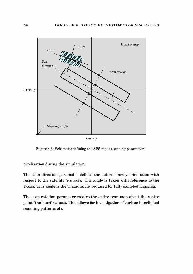
84 CHAPTER 4. THE SPIRE PHOTOMETER SIMULATOR
Map origin (0,0)
centre_z
centre_y
Scan direction
Input sky map
Scan rotation
z axis y axis
Figure 4.5: Schematic defining the SPS input scanning parameters.
pixelisation during the simulation.
The scan direction parameter defines the detector array orientation withrespect to the satellite Y-Z axes. The angle is taken with reference to theY-axis. This angle is the ‘magic angle’ required for fully sampled mapping.
The scan rotation parameter rotates the entire scan map about the centrepoint (the ‘start’ values). This allows for investigation of various interlinkedscanning patterns etc.
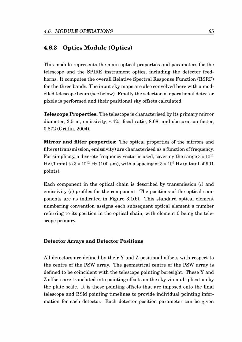
4.6. MODULE OPERATIONS 85
4.6.3 Optics Module (Optics)
This module represents the main optical properties and parameters for thetelescope and the SPIRE instrument optics, including the detector feed-horns. It computes the overall Relative Spectral Response Function (RSRF)for the three bands. The input sky maps are also convolved here with a mod-elled telescope beam (see below). Finally the selection of operational detectorpixels is performed and their positional sky offsets calculated.
Telescope Properties: The telescope is characterised by its primary mirrordiameter, 3.5 m, emissivity, ∼4%, focal ratio, 8.68, and obscuration factor,0.872 (Griffin, 2004).
Mirror and filter properties: The optical properties of the mirrors andfilters (transmission, emissivity) are characterised as a function of frequency.For simplicity, a discrete frequency vector is used, covering the range 3×10¹¹
Hz (1 mm) to 3×10¹² Hz (100 µm), with a spacing of 3×10⁹ Hz (a total of 901points).
Each component in the optical chain is described by transmission (t) andemissivity (e) profiles for the component. The positions of the optical com-ponents are as indicated in Figure 3.1(b). This standard optical elementnumbering convention assigns each subsequent optical element a numberreferring to its position in the optical chain, with element 0 being the tele-scope primary.
Detector Arrays and Detector Positions
All detectors are defined by their Y and Z positional offsets with respect tothe centre of the PSW array. The geometrical centre of the PSW array isdefined to be coincident with the telescope pointing boresight. These Y andZ offsets are translated into pointing offsets on the sky via multiplication bythe plate scale. It is these pointing offsets that are imposed onto the finaltelescope and BSM pointing timelines to provide individual pointing infor-mation for each detector. Each detector position parameter can be given
86 CHAPTER 4. THE SPIRE PHOTOMETER SIMULATOR
a slight random scatter if manufacturing errors are required to be repre-sented.
Each detector is assigned a number defined by its position within the arrayand shown in Figure 4.6. Numbers start at 0 and run to 138 in the caseof the PSW array. Numbering begins at the bottom left of the array andincreases as shown. Additional pixels such as dark pixels and thermometersare appended to the end of this number sequence.
Z
8
7
6
5
4
3
2
1
0
16
15
14
13
12
11
10
9
25
24
23
22
21
20
19
18
17
33
32
31
30
29
28
27
26
42
41
40
39
38
37
36
35
34
Figure 4.6: Diagram showing the indexing system used to specify individual detec-tor pixels within the SPS.
Beam profiles: Each detector has a beam profile on the sky, representedby a modelled telescope beam, computed using a Hankel transformation.An example of the modelled beam used in the SPS is shown in Figure 4.7.In the current version, all detectors in a given array have the same beamprofile. The module architecture allows the beam profiles to be specifiedindependently for different detectors.
Feedhorn throughput: Since each feedhorn is single moded, the opticalthroughput (AΩ) is nominally equal to λ2 (Griffin et al., 2002a).
Spillover efficiency: This is the fraction, ηs, of the throughput from a de-tector that illuminates the telescope. A fraction 1-ηs is assumed to terminateon the walls of the level-1 enclosure. The value of ηs is assumed to be thesame for all detectors in a given array.
Feedhorn/cavity efficiency: Each detector has an optical efficiency, ηfeed,
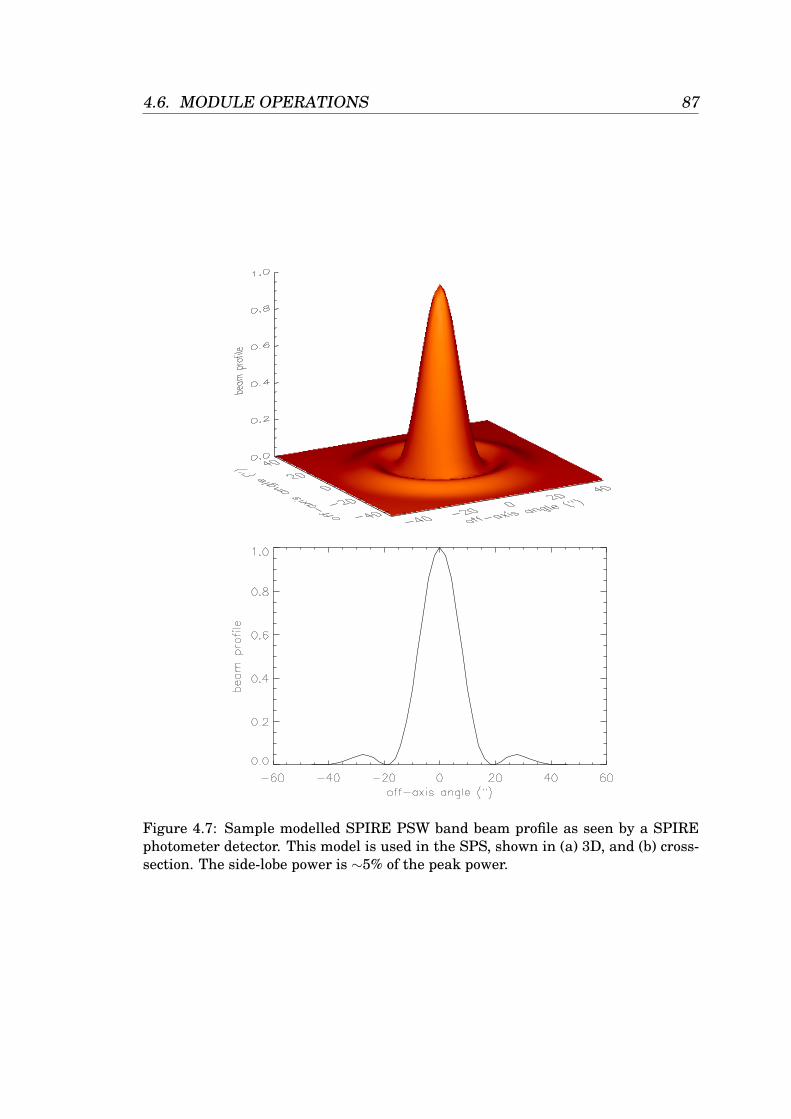
4.6. MODULE OPERATIONS 87
Figure 4.7: Sample modelled SPIRE PSW band beam profile as seen by a SPIREphotometer detector. This model is used in the SPS, shown in (a) 3D, and (b) cross-section. The side-lobe power is ∼5% of the peak power.
88 CHAPTER 4. THE SPIRE PHOTOMETER SIMULATOR
equal to the fraction of the horn throughput (AΩ) which is absorbed by thebolometer.
Cutoff wavelength: Each detector feedhorn has an output waveguide withdiameter dwav, which determines the cutoff wavelength.
Module operation: This module operates in a non-time-stepping mode. Alloptical element transmission and emissivity profiles are contained in inputfiles. The path and name of these files is stored within an input file specifiedby the user. The order of the input files represents the order of the opticalchain, beginning with the primary mirror and increasing towards the detec-tor array.
Transmission matrices are initialised for each waveband based on the inputdata (e.g. the number of optical elements in the system, and their order inthe optics chain) and associated pointers are assigned. The transmissioncalculator function, set within the optics code is then stepped through oncefor each waveband, producing the output transmission array. This array canbe used to find the overall transmission between any two points in the opticschain.
Convolved input sky maps are produced using a pre-modelled telescope beampattern kernel. A beam model equivalent in resolution to that of the inputmap is used. Pre-modelled beams exist for input map resolutions from 1 to6′′/pixel in integer steps (input maps must match this resolution, i.e. be ininteger arcsec steps).
Finally the chosen detector array pixels are identified from the user inputand their sky positional offsets calculated. Selection is carried out via agraphical user interface (array-gui.pro), which allows selection of individualdetectors, or a choice of either full arrays or all co-aligned pixels. Opting touse less detector pixels results in a faster run time, however a minimum ofone pixel must be selected in each array.
4.6. MODULE OPERATIONS 89
4.6.4 Thermal System (Thermal)
This module characterises the temperatures of all relevant elements andtheir time variations. A vector of temperature differences verses time de-scribes thermal drifts of elements within the system for the timeline dura-tion. The thermal noise originates from 3He stage fluctuations. This time-line is used as an input to the detector model (To parameter).
Module operation
Origin of thermal fluctuations: Thermal fluctuations are expected to be asource of correlated noise within the SPIRE instrument. Correlated noise inthis case refers to noise common to all detectors and experienced simultane-ously, or near simultaneously. This does not however mean that the responseof each detector to this noise is equal (see the detectors module documenta-tion within Sibthorpe and Griffin (2006)). There are many sources that con-tribute to the overall thermal fluctuations within the system, however theirresultant impact can be modelled as a single thermal noise timeline. This isreasonable for the case of the SPS, as it is the effect on the detector outputthat is of interest.
Modelling method: We have chosen to take the 3He cooler as the primarysource of thermal fluctuations. A 1/f noise timeline is simulated with a giventhermal noise spectral density, with units of KHz−1/2, and 1/f noise kneefrequency, fk, with units of Hz.
The bolometer detector arrays (BDA) within SPIRE are connected to thecooler via a series of cold straps. In addition to this the detector arraysthemselves are directly coupled to a large thermal mass of the invar mount.As a consequence of this, any thermal fluctuations arising in the cooler arelow-pass filtered by the time they reach the bolometers. This is modelledhere using a first order low pass filter profile, with a different time constant,in seconds, for each array. The different time constants represent the differ-ent ways in which the thermal noise could manifest itself in each array. Theinput thermal noise timeline remains fixed for each array, but the filteringchanges the thermal noise timeline seen by the three detector arrays.
90 CHAPTER 4. THE SPIRE PHOTOMETER SIMULATOR
Given the difficultly in accurately predicting the operational thermal envi-ronment of SPIRE, the nominal values to be used within the SPS are chosenso as to present a challenging task for data analysis systems. This will as-sist in the development of robust data analysis tools. Values for the thermalnoise spectral density, 1/f noise knee frequency, and three time constantsare required. The noise spectral density is be given a value higher than thatexpected from most 3He fridges. This value should also be set so as to pro-duce a noise timeline with large-scale deviations several times those arisingfrom independent detector 1/f noise sources alone. It was found that a valueof 50 µKHz−1/2 works well.
To produce significant variation within a single scan line, a 1/f noise kneefrequency of approximately 30 mHz is currently used. This allows for ap-proximately four 1/f noise timescales to pass during a 1 degree scan line,scanning at the nominal rate of 30′′s−1. It also sets the thermal 1/f noiseknee close to the detector 1/f noise knee, making the identification of onefrom the other a more challenging task.
Thermal time constants have been estimated from instrument test results.Values range from 70 - 130 s, with a nominal value of 100 s. From thisthe chosen nominal SPS values are currently 70, 100, and 130 s, for thephotometer short, medium, and long wavelength arrays respectively.
Implementation: The initial 1/f noise time line is produced using the stan-dard SPS 1/f noise timeline generator (see Sibthorpe and Griffin (2006) forinformation). The Fourier transform of this timeline is then performed, andthe resultant frequency spectrum multiplied by the appropriate first orderfilter profile. The inverse transform is then performed to return the finalthermal noise timeline.
This noise timeline is input to the bolometer model as an addition to thedetector array base temperature, To.
Sample data: Figure 4.8 shows a sample detector output voltage timeline.This timeline shows the result of an input thermal drift, generated as out-lined above (red line), with input parameters of 50 µKHz−1/2 thermal stabil-ity, fk = 30 mHz, and t = 70 s, for a single PSW detector. Significant thermal
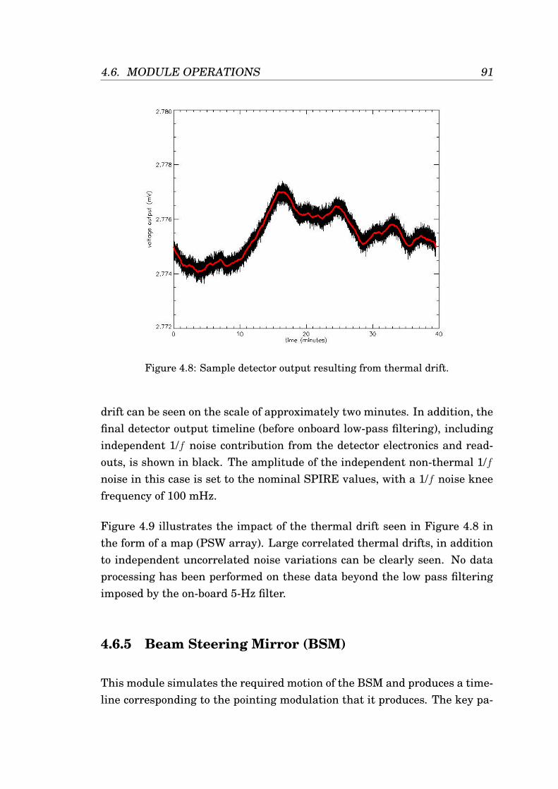
4.6. MODULE OPERATIONS 91
Figure 4.8: Sample detector output resulting from thermal drift.
drift can be seen on the scale of approximately two minutes. In addition, thefinal detector output timeline (before onboard low-pass filtering), includingindependent 1/f noise contribution from the detector electronics and read-outs, is shown in black. The amplitude of the independent non-thermal 1/fnoise in this case is set to the nominal SPIRE values, with a 1/f noise kneefrequency of 100 mHz.
Figure 4.9 illustrates the impact of the thermal drift seen in Figure 4.8 inthe form of a map (PSW array). Large correlated thermal drifts, in additionto independent uncorrelated noise variations can be clearly seen. No dataprocessing has been performed on these data beyond the low pass filteringimposed by the on-board 5-Hz filter.
4.6.5 Beam Steering Mirror (BSM)
This module simulates the required motion of the BSM and produces a time-line corresponding to the pointing modulation that it produces. The key pa-
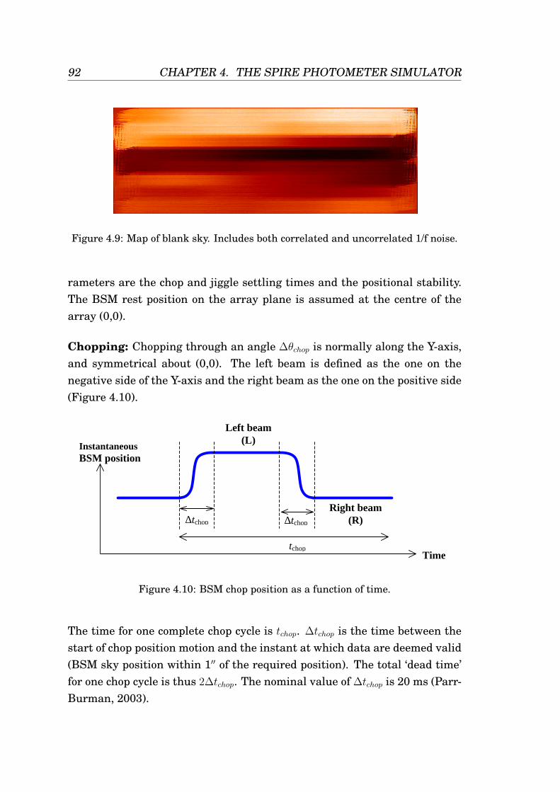
92 CHAPTER 4. THE SPIRE PHOTOMETER SIMULATOR
Figure 4.9: Map of blank sky. Includes both correlated and uncorrelated 1/f noise.
rameters are the chop and jiggle settling times and the positional stability.The BSM rest position on the array plane is assumed at the centre of thearray (0,0).
Chopping: Chopping through an angle ∆θchop is normally along the Y-axis,and symmetrical about (0,0). The left beam is defined as the one on thenegative side of the Y-axis and the right beam as the one on the positive side(Figure 4.10).
Instantaneous BSM position
Time
Left beam (L)
Right beam (R) ∆tchop ∆tchop
tchop
Figure 4.10: BSM chop position as a function of time.
The time for one complete chop cycle is tchop. ∆tchop is the time between thestart of chop position motion and the instant at which data are deemed valid(BSM sky position within 1′′ of the required position). The total ‘dead time’for one chop cycle is thus 2∆tchop. The nominal value of ∆tchop is 20 ms (Parr-Burman, 2003).
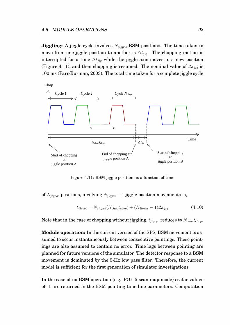
4.6. MODULE OPERATIONS 93
Jiggling: A jiggle cycle involves Njigpos BSM positions. The time taken tomove from one jiggle position to another is ∆tjig. The chopping motion isinterrupted for a time ∆tjig while the jiggle axis moves to a new position(Figure 4.11), and then chopping is resumed. The nominal value of ∆tjig is100 ms (Parr-Burman, 2003). The total time taken for a complete jiggle cycle
Start of chopping at
jiggle position A
End of chopping at jiggle position A
Start of chopping at
jiggle position B
Cycle 1 Cycle 2 Cycle Nchop
∆tjig Nchoptchop Time
Chop position
Figure 4.11: BSM jiggle position as a function of time
of Njigpos positions, involving Njigpos − 1 jiggle position movements is,
tjigcyc = Njigpos(Nchoptchop) + (Njigpos − 1)∆tjig (4.10)
Note that in the case of chopping without jiggling, tjigcyc reduces to Nchoptchop.
Module operation: In the current version of the SPS, BSM movement is as-sumed to occur instantaneously between consecutive pointings. These point-ings are also assumed to contain no error. Time lags between pointing areplanned for future versions of the simulator. The detector response to a BSMmovement is dominated by the 5-Hz low pass filter. Therefore, the currentmodel is sufficient for the first generation of simulator investigations.
In the case of no BSM operation (e.g. POF 5 scan map mode) scalar valuesof -1 are returned in the BSM pointing time line parameters. Computation
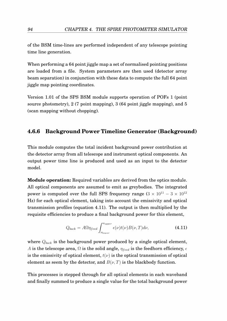
94 CHAPTER 4. THE SPIRE PHOTOMETER SIMULATOR
of the BSM time-lines are performed independent of any telescope pointingtime line generation.
When performing a 64 point jiggle map a set of normalised pointing positionsare loaded from a file. System parameters are then used (detector arraybeam separation) in conjunction with these data to compute the full 64 pointjiggle map pointing coordinates.
Version 1.01 of the SPS BSM module supports operation of POFs 1 (pointsource photometry), 2 (7 point mapping), 3 (64 point jiggle mapping), and 5(scan mapping without chopping).
4.6.6 Background Power Timeline Generator (Background)
This module computes the total incident background power contribution atthe detector array from all telescope and instrument optical components. Anoutput power time line is produced and used as an input to the detectormodel.
Module operation: Required variables are derived from the optics module.All optical components are assumed to emit as greybodies. The integratedpower is computed over the full SPS frequency range (3 × 10¹¹ − 3 × 10¹²
Hz) for each optical element, taking into account the emissivity and opticaltransmission profiles (equation 4.11). The output is then multiplied by therequisite efficiencies to produce a final background power for this element,
Qback = AΩηfeed
∫ νupper
νlower
ε(ν)t(ν)B(ν, T )dν, (4.11)
where Qback is the background power produced by a single optical element,A is the telescope area, Ω is the solid angle, ηfeed is the feedhorn efficiency, εis the emissivity of optical element, t(ν) is the optical transmission of opticalelement as seem by the detector, and B(ν, T ) is the blackbody function.
This processes is stepped through for all optical elements in each wavebandand finally summed to produce a single value for the total background power
4.6. MODULE OPERATIONS 95
in each waveband. It is assumed that the incident background power is thesame for each detector within an array is equal.
4.6.7 Astronomical Power Timeline Generator (Astropower)
This module calculates the timelines for the absorbed astronomical signalpower for each detector.
Module operation: Following the initialisation of the required variables, aconvolved sky map is formed, either by convolution of the given sky map witha simulated telescope beam, or by direct loading into memory a convolvedsky map data file (this can be done if the sky map being used has previouslybeen convolved and stored).
The power measured at the detector for each scanning point is then found bytaking a 2D linear interpolation of the convolved sky map for each observa-tion scan position. This is then multiplied by the appropriate transmissionprofile to give the power at the detector. These values are then integratedover the frequency range using Simpson’s rule and multiplied by the nec-essary efficiency factors and constants resulting in an astronomical powervalue. The output is an array, for each waveband, of the total astronomicalpower at the detector for each scan point observed.
The total astronomical signal power falling on a detector in a single timestep is given by,
Qsig = AΩηfeedηtelSν10−26
∫ νupper
νlower
t(ν)dν, (4.12)
where Qsig is the astronomical power in W from a source, and Sν is the fluxreceived from the source in Jy.
96 CHAPTER 4. THE SPIRE PHOTOMETER SIMULATOR
4.6.8 Detector Voltage Timeline Generator (Detectors)
This module models the detector response to an input background and as-tronomical power via a full physical model of the system. The model usedis based on the work of Sudiwala et al. (1992), and is implemented in orderto generate realistic bolometer responses for the flight detector arrays. Thisincludes the ability to generate a non-linear output in response to a suffi-ciently high power input. In addition, measured flight detector parameterscan be input, thereby generating a unique response to any system variation,such as fluctuation in thermal environment, for each bolometer.
Bolometer response: The detector module requires initialisation before itcan be used to begin an observation. This is due to the fact that in orderto perform an observation, operating points on the bolometer load curvesmust first be defined and set into the common blocks used to store detectormodule parameters. Subsequent time steps compare new inputs with thosefrom a previous time step in order to determine the level of change within thesystem, and hence the bolometer response, before computing a new output.
In cases where key parameters change, such as the detector array base platetemperature or background power, a recalculation of each bolometer operat-ing point is required. The operating point is found using a Newton Raphsonmethod to compute the correct bias parameter. A bias parameter is set andthe associated bias voltage for that parameter found. This is then comparedto the actual bias voltage set within the system. Once the bias voltage asso-ciated with the bias parameter is within some tolerance, the operating pointis obtained. Each time a new operating point is calculated, new values forresponsivity and detector time constant are derived, and used in the compu-tation of the detector response.
In cases of high astronomical signal the detector response will become non-linear. A threshold is set for this condition, the value being set from tests oras a compromise for computational power. Up until this threshold is reachedthe previous operating point and associated parameters are assumed to beconstant, and a linear response computed. In cases where the astronomi-cal signal becomes greater than a small fraction of the nominal background
4.6. MODULE OPERATIONS 97
power (∼ 5%), the detector’s operating point and parameters are recalcu-lated, and the new operating point is compared to the previous voltage andtaken as the new voltage change (dV ). The time constant is taken to be themean of the time constant at each operating point.
Noise: Noise spectral density estimates are made for each detector indepen-dently via a series of equations as formulated by Sudiwala et al. (1992). Thenoise estimate is made based on the initial bolometer parameters. Only onevalue of noise spectral density is computed for any individual detector. Thenoise estimates include contributions from photon noise arising from the pri-mary and secondary mirrors (background power dominated), phonon noise,load resistor noise, Johnson, and amplifier noise. These replicate the noisesources specified in the SPIRE sensitivity document (Griffin, 2004).
These noise estimates are used as inputs to a noise time line generator. Thenoise generator uses this noise estimate along with a 1/f noise knee fre-quency to output a unique 1/f noise time line for each detector. The 1/fpower spectrum is imposed in Fourier space via multiplication with a whitenoise time line. The white noise has a Gaussian probability distribution withthe RMS value set to en
√∆f , where en is the overall noise spectral density,
and ∆f is the frequency bandwidth corresponding to the specified simulatortime step.
Bolometer parameters: There are two options when selecting the bolome-ter parameters to be used within the detector model. The first assumes thateach detector is identical, giving every bolometer the same nominal bolome-ter parameters for a given array. The second option is to use the individualmeasured bolometer parameters. These are read in from a parameters file.The choice is made by selecting either to have the ‘real bolometer parame-ters’ on or off (1/0) in the detectors parameters file (params-detectors.txt).
Operating with the real bolometer parameters also provides the measuredvalues of 1/f noise knee frequency for each detector. These values are usedas a series of offset values from the SPIRE nominal detector knee frequency(0.1 Hz). For example, when the nominal knee frequency is set to 0.1 Hz, therealistic values are set. In the case where the knee frequency is set to 1 Hz,the same scatter will be seen but with 1 Hz added to each value.

98 CHAPTER 4. THE SPIRE PHOTOMETER SIMULATOR
4.6.9 Sampling System (Sampling)
This module low-pass filters and samples the output detector data time line.The data are sampled at the rate specified by the user. This system repli-cates the SPIRE on-board 5-Hz analogue filter within the physical system.
Module operation: Each detector voltage time line is filtered by multipli-cation in Fourier space with the 5-Hz filter profile.
The data are then sampled at a given frequency, where the sampling fre-quency is lower than the simulator step frequency. A linear interpolationis performed when a sampling point does not match an integer number ofsimulator time steps.
4.6.10 Simulator Operation
There are currently two modes of SPS operation, standard, and repeat. Stan-dard is classed as operating mode 0. This setting will perform n number ofsimulations in full. Repeat mode (1) performs one full simulation. Oncecomplete, new detector noise realisations and filtering is performed and im-posed on the detector model output of the initial simulation. This is intendedfor fast generation of data sets in cases such as high redshift extra-galacticstudies, where many maps of the same region will be required. The out-put from these simulations can not therefore include variations in systempointing or detector temperature. As a result these data have a lower orderrepresentation of the SPIRE system.
The current version runs a full simulation in mode 0 in approximately halfthe time of the real life observation, on a typical desktop computer (CPUspeed ∼P4 2.7 GHz). The output file size varies depending on the output op-tions selected, but a one square degree scan map simulation with two typesof output time-line (e.g. sampled and noiseless data) will be ∼ 400 MB.
4.7. CHAPTER SUMMARY 99
4.7 Chapter Summary
In this chapter, I have introduced the SPIRE photometer software simulator,and outlined its primary goals and operation. The SPS is a highly realisticsoftware model of the SPIRE photometer, which in the current version, con-tains all of the primary photometer subsystems. It is capable of simulatingthe photometer system operation, and data characteristics. A brief descrip-tion of the methods used to model each instrument subsystem, implementedin the form of a module, has also been presented. The limitations of the sim-ulations have been noted, specifically, that results from simulation can onlybe representative, and not identical to, the final system output. This makesthe simulator useful in understanding the impact of the known systematicson the data quality, but it cannot predict the final instrument performanceuntil the system is in orbit.

100 CHAPTER 4. THE SPIRE PHOTOMETER SIMULATOR
Chapter 5
SPIRE Data Reduction and SPSPerformance Verification
The SPIRE photometer simulator produces as its primary output three kindsof time ordered data (TOD) time-lines, the telescope pointing time-line, BSMposition time-line, and detector voltage time-line. In order for the simulatorto be useful, it is crucial that the system operation be verified. Correct op-eration can be assessed by comparing the output signal and noise levels forsample cases with the theoretical values. This in turn requires the reduc-tion of the TOD to some useful form, such as a map. The data should also becleaned of instrumental and astronomical characteristics which might intro-duce error which cannot be easily accounted for theoretically. This cleaningwill represent the kind of processes performed in a pre-map-making datapipeline.
In this chapter an overview of the data cleaning methods, through whichSPIRE data must be processed, are presented. A brief introduction to naıveand maximum likelihood map-making methods is also given. Following this,a robust method for the determination of the SNR of a point source, in a mapcontaining uniform noise, is presented. This method is then used to derivethe SNR of a source within a SPS output map. The SNR obtained is thenused to validate the SPS operation, by comparison with the theoreticallyexpected value, and by comparison with the SPIRE sensitivity model (Grif-
101
102CHAPTER 5. DATA REDUCTION AND SIMULATOR VERIFICATION
fin, 2004). Finally, an aside on the SPIRE map-making selection exercise ispresented.
5.1 Data Cleaning
Raw detector TOD contain a range of different artefacts which require clean-ing before any data analysis can be performed. Cosmic rays hitting the de-tector array for example will cause a large signal spike, or ‘glitch’, in thesignal timeline. It may take several time constants for the detector to re-turn to a normal operating level following such a hit. Often these artefactsare dealt with by identifying the cosmic ray hit and flagging this section ofdata as ‘bad’ for a certain number of time constant after its detection. Inmany cases these missing data are then filled using some interpolation ofthe surrounding data, with the correct characteristic noise being input. Thismakes it possible to perform other data analysis processes, such as Fouriertransforms, without the missing data resulting in new artifacts.
A clean telescope pointing solution must also be obtained from the raw TOD.Herschel has an absolute pointing error requirement of 3.7′′. An additionaldrift on this initial error will occur throughout an observation and is a func-tion of time. It is expected that a pointing calibration will be performed atthe beginning of each observation, and possibly during long observations,with the time period depending on the final telescope pointing stability. Thecalibration will be performed by the system using two star tracker camerasfacing backwards on the Herschel service module. These cameras will alsotrack the telescope throughout the observation, and their data telemeteredto the ground. These data can be used for a posteriori pointing reconstruc-tion. These data do not however, feedback to the telescope systems to correctany pointing drifts which might occur during an observation.
Common mode noise, i.e. correlated 1/f noise, will also be removed at atthe data cleaning stage by the data reduction pipeline. The major source ofcommon mode noise is expected to be long time scale thermal drifts, origi-nating in the 3He cooler, especially immediately after fridge recycle. These
5.1. DATA CLEANING 103
are passed on to the BDAs resulting in a corresponding drift detector outputvoltage (see Section 1.4). Due to the individual bolometer parameters asso-ciated with each detector, the resultant change in operation will vary fromdetector to detector. Data from the two thermometers located within eachBDA can be used to monitor the thermal drifts, and used as an input to thebolometer thermal model of (Sudiwala et al., 1992). By working this modelbackwards, and applying the previously measured parameters for each de-tector, it is possible to remove the effects of the thermal drifts for each detec-tor, to the accuracy of the thermometer measurement. In practice many ofthe common mode noise signals may contain a partial correlation across thedetector array, caused by a temperature gradient. Therefore some phase lagmay need to be introduced in the application of the thermometry data.
In addition to thermal drifts within the BDA, there may be drifts in the tem-perature, and therefore emission, of some cold optical components, therebycausing a variation in optical loading on the detectors. This will act as an-other source of common mode noise. It is drifts in the components in theLevel-1 temperature stage (5-K) that will cause the significant error, espe-cially to PLW observations, due to their high temperature.
Other optical components will also experience temperature fluctuations andthus will give rise to similar correlated noise. The scale of the variations willhowever again be small, and on long time scales. A particularly significantsource of correlated noise from the optics system would be from variations inthe telescope primary and secondary mirrors, were it not for the long ther-mal time constant of these components, expected to be significantly longerthan the observing time of a typical observation.
Finally the data will require flat-fielding. The responsivity of each detectorwill be different, even when operating in a stable environment. As a result adifferent signal level will be measured by each detector when observing thesame source. These differences must be calibrated out in order to co-add allof the detector timelines within an array, and produce an accurate flux cali-bration. This is done by multiplying each detector timeline by a gain factor,or flat-field. The flat-field is often derived from observations of a blank partof the sky, or the inside of a telescope dome. In the case of Herschel-SPIRE,
104CHAPTER 5. DATA REDUCTION AND SIMULATOR VERIFICATION
the flat-field can be derived initially from measurements of the detector re-sponsivity, and use of the bolometer thermal model and measured bolometerparameters, but will be verified and enhanced by observations of astronomi-cal sources.
For SPIRE, it is not critical to deal with the removal of the detector responsefunction. While the output data timeline will be a convolution of the as-tronomical sky signal with the detector (R-C style) response function, this isonly a minor issue. The detector time constants are sufficiently fast, that thedominating factor in the response of a detector to a step change in signal, isthe 5-Hz low pass filter.
Observations that involve chopping or nodding require a further stage ofpreprocessing, before a map can be made. Both the chop and nod cycles mustbe demodulated. In the simplest case, this can be done by integrating thetotal signal in one chop half, and subtracting it from the subsequent chophalf. This gives the total change in signal between the on, and off sourcepositions, i.e. the astronomical signal. The signal is then averaged overchop cycles. The error in this measurement can be taken as the standarddeviation of the signal values. Telescope nodding can also be demodulatedin a similar way.
Each one of these data processing techniques is likely to result in some lossof information, as no routine will be perfect. Also, it is highly likely thatdata from the in-flight system will contain various other, as yet unknown,systematic artefacts. These will also need to be dealt with at this stage ofdata processing.
There is a huge range of data analysis techniques which can be appliedto perform these tasks, and many more being continually developed. TheSPIRE data reduction pipeline is currently being designed to carry out thesecorrections. The SPS will be used to evaluate the efficiency and accuracy ofthis software. To date, however, simulations have been carried out assum-ing that such systematic effects can be successfully eliminated, in order toevaluate the basic observing modes, the effects of known noise contributionsthat will not be dealt with by the pipeline, and map making routines.
5.2. CALIBRATION 105
5.2 Calibration
In general, calibration of the data can be performed at any stage of dataprocessing. If the detector system used has a linear response, a calibrationconstant, with units of Jy/V, can be derived, simply by observing a sourceof known flux. This constant can then be applied to the entire data set,converting the data from V to Jy. As well as the responsivity of the detector,this constant takes into account all gain factors between the detector andthe output.
In the case of a bolometer, the responsivity is a function of detector operatingtemperature, bias, and radiant background, and therefore the calibrationconstant will only be correct for given conditions. If the temperature of thedetectors is known, then it is possible to use a thermal model (Sudiwalaet al., 1992) to calculate the corresponding responsivity.
In addition to these dependences, bolometers also have a non-linear response.At low signal levels the deviation from linearity is small and can be ignored;however at high signals it can become an issue. Given the appropriate pa-rameters, this non-linear response can again be modelled, and an appropri-ate calibration applied (see Section 1.4).
Studies performed thus far with SPS data have not implemented thermaldrifts. Therefore it has been possible to derive a calibration constant for thenominal detector operating conditions. In cases where a simulation containsa very bright source, a separate calibration curve has been used to calibratethe data. This calibration curve was produced using the simulator’s responseto a series of sources of known flux. The chosen fluxes ranged from the linearto the highly non-linear regime.
5.3 Map-Making
Once cleaned the data must be converted from TOD to a map. There is arange of map-making methods, the more complex of which are summarised
106CHAPTER 5. DATA REDUCTION AND SIMULATOR VERIFICATION
in Tegmark (1997), that can be applied depending on the noise character-istics. The simplest form of map making can be achieved by binning thedata into a grid, and assigning to each pixel a value equal to the mean ofthe samples falling within it. This is referred to as a ‘naıve map’. In thepresence of 1/f noise however, striping may be seen along the scan direction.Other map-making methods attempt, through a variety of techniques, todeal with this 1/f noise during the map-making process. In many cases thetechnique implemented is science case dependent, and thus requires thatsome assumption is made regarding the information contained within thedata. In the case of point source studies, it is generally sufficient to high-pass filter the TOD to remove the 1/f noise drifts, as the majority of theinformation relating to this source type is contained at high frequencies.
In this section we will outline a commonly used maximum likelihood method,also referred to as the ‘COBE’ method, which attempts to deal with 1/f noisewithout the requirement to make assumptions about the underlaying data.This case is in essence a χ2 minimisation given by:
χ2 =∑i,i′
(di −∑p
Ai,pmp)N−1i,i′ (di′ −
∑p′
Ai′,p′mp′), (5.1)
where di is the ith data sample and mp is value of the map pixel p. Notethat m is being treated as a 1D vector. Ni,i′ is the time-time noise covariancematrix, given by Ni,i′ = 〈(di−µi)(di′ −µi′)〉, where µ is the mean. This matrixeffectively measures the noise correlation between sample i, and sample i′.Ai,p is the pointing matrix and has dimensions of nsamples × npixels. This is asparse matrix, containing a value of 1 where there is a sample, and zero inall other locations. This matrix can be used to turn a map in to a timelineand vice-versa.
The minimisation of this expression can be represented as:
0 =∂χ2
∂mp
=∑i,i′
(−Ai,p)N−1i,i′ (di′ −
∑p′
Ai′,p′mp)
5.3. MAP-MAKING 107
+∑i,i′
(di −∑p
Ai,pmp)N−1i,i′ (−Ai′,p)
= −2∑i,i′
Ai,pN−1i,i′ (xi′ −
∑p′
Ai′,p′mp′), (5.2)
which when converted to matrix notation becomes:
ATN−1Am = ATN−1d
⇒ m = (ATN−1A)−1ATN−1d. (5.3)
Solving this generalised least squares equation for m will produce the max-imum likelihood map. However, this is not easy in practice. Even for mapsof modest size, the memory and computational power required to store andinvert the matrices involved is beyond that currently available. In order togenerate a one square degree SPIRE scan map using this direct method, amatrix containing approximately three billion points would have to be storedand inverted. This matrix would be ∼46 GB, and the inversion would not bepossible. This problem has been tackled in a variety of ways. It is often as-sumed that the noise properties are stationary, i.e. that the noise level, and1/f knee frequency is constant over some period of time. This, along withvarious other assumptions regarding the covariance matrix, such as the ma-trix being Toeplitz, can be used, simplifying the matrix inversion method.Almost all methods use some form of iterative scheme, generating at first anaıve map. This map is used to refine the covariance matrix, and a moreaccurate map is produced. This continues until either a fixed number of iter-ations has been performed, or some convergence criterion has been met. SeeChristopher (2002), and Crill and Netterfield (in prep.), for good reviews ofimplementation methods.
It should be noted that multiple observations of the same region of sky, withthe region being revisited on a variety of time scales, is required to derive amaximum likelihood map in this way. This type of observation is known ascross-linking, and provides redundancy in the data. Random cross-linking
108CHAPTER 5. DATA REDUCTION AND SIMULATOR VERIFICATION
provides the best results (Tegmark, 1997).
5.4 Simulator Performance Verification
Individual SPS modules and subsystems were independently verified duringdevelopment. In addition, it was important to confirm that the entire sys-tem worked as predicted by theory. The modelled voltage response from theSPS bolometer module was compared to the SPIRE sensitivity model (Grif-fin, 2004) and found to agree well for a given source flux. Since the signaland noise time-lines are generated independently, the measurement of theSNR of a point source provides a robust test of the entire system. The noiseequivalent flux density (NEFD) can be used to predict the SNR of a sourceof flux density Sν , when observed for time tint. The NEFD is defined as thesource flux density that will provide a SNR of 1 in an integration time of 1/2s, and for SPIRE is given by Equation 5.4.
NEFD =NEP
ηηfiltAtel∆ν, (5.4)
where NEP is the detector noise equivalent power, Atel is the area of thetelescope, η is the product of the system efficiency factors, e.g. feedhornthroughput, spill over efficiency, telescope obscuration factor etc., ∆ν is thefilter band width, and ηfilt(ν) is transmission efficiency of the system opticalcomponents.
The test results from the simulator were compared to the standard SPIREperformance model (Griffin, 2004). The appropriate 5σ-1 hour sensitivityvalues when observing in scan map mode were used for comparison.
5.4.1 Point Source SNR Measurement
Consider here a telescope whose beam profile (response to a scan of a pointsource) is a Gaussian. The resultant map from such an observation wouldbe a Gaussian embedded in a noisy map with a signal, in each pixel i, of Si,
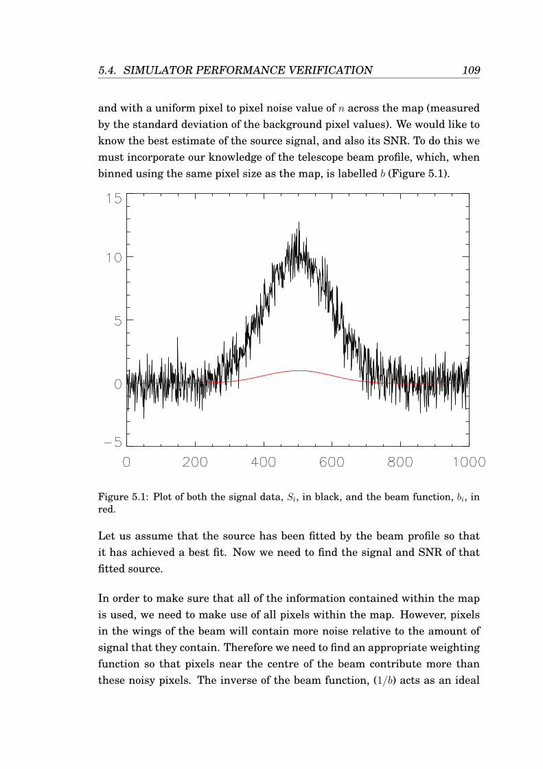
5.4. SIMULATOR PERFORMANCE VERIFICATION 109
and with a uniform pixel to pixel noise value of n across the map (measuredby the standard deviation of the background pixel values). We would like toknow the best estimate of the source signal, and also its SNR. To do this wemust incorporate our knowledge of the telescope beam profile, which, whenbinned using the same pixel size as the map, is labelled b (Figure 5.1).
Figure 5.1: Plot of both the signal data, Si, in black, and the beam function, bi, inred.
Let us assume that the source has been fitted by the beam profile so thatit has achieved a best fit. Now we need to find the signal and SNR of thatfitted source.
In order to make sure that all of the information contained within the mapis used, we need to make use of all pixels within the map. However, pixelsin the wings of the beam will contain more noise relative to the amount ofsignal that they contain. Therefore we need to find an appropriate weightingfunction so that pixels near the centre of the beam contribute more thanthese noisy pixels. The inverse of the beam function, (1/b) acts as an ideal
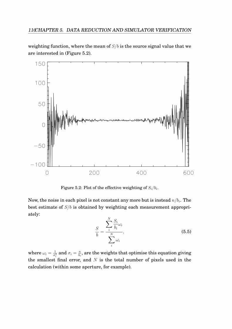
110CHAPTER 5. DATA REDUCTION AND SIMULATOR VERIFICATION
weighting function, where the mean of S/b is the source signal value that weare interested in (Figure 5.2).
Figure 5.2: Plot of the effective weighting of Si/bi.
Now, the noise in each pixel is not constant any more but is instead n/bi. Thebest estimate of S/b is obtained by weighting each measurement appropri-ately:
S
b=
N∑i
Sibiωi
N∑i
ωi
, (5.5)
where ωi = 1σ2
iand σi = n
bi, are the weights that optimise this equation giving
the smallest final error, and N is the total number of pixels used in thecalculation (within some aperture, for example).
5.4. SIMULATOR PERFORMANCE VERIFICATION 111
Equation 5.5 leads to:
S
b=
N∑i
Sibi
b2in2
N∑i
b2in2
. (5.6)
The final error in this measurement is then defined as
1
σ2best
=2∑i
1
σ2i
=N∑i
ωi
(5.7)
⇒ σbest =1√√√√ N∑i
ωi
=1√√√√ 1
n2
N∑i
b2i
=n√√√√ N∑i
b2i
. (5.8)
Thus the SNR is simply
SNR =
N∑i
Sibi
N∑i
b2i
·
√√√√ N∑i
b2i
n=
N∑i
Sibi
n
√√√√ N∑i
b2i
. (5.9)
This has two main advantages over other methods for calculating signal tonoise. The first is that it produces an estimate that is independent of boththe size of the pixel used in the map, and the size of the aperture placedaround the source. The first point can be demonstrated by seeing how eachterm in the above expression varies with the pixel size.
If L is the pixel size then:
N∑i
Sibi ∝ 1
L2,
N∑i
b2i ∝ 1
L2,
n ∝ 1
L. (5.10)
112CHAPTER 5. DATA REDUCTION AND SIMULATOR VERIFICATION
Therefore:
SNR ∝
1
L2
1
L· 1
L
= constant. (5.11)
The second point can be seen by considering an annulus that is increasedin size, beyond the extent of the beam profile. As the annulus increases insize the new pixels that are encompassed contain only noise and no signal.Therefore these pixels are weighted such that they contribute nothing to thefinal measurement, and so have no effect on the derived signal to noise ratio.The best signal to noise is then obtained by selecting an annulus that is bigenough to contain all of the significant beam profile.
Additionally the beam profile does not need to be normalised so that it matchesthe amplitude of the signal. So long as it is centred on the position of thesource, the final signal to noise ratio will be independent of the beam nor-malisation. To obtain the final source signal, the measurement in Equation5.6 must be multiplied by the peak value of b.
These equations are only applicable when the noise in the map can be takenas uniform. In the case of non-uniform noise, such as 1/f noise, these expres-sions are only approximate. In this case we need to replace n with ni in allthe calculations. This results in an expression for the signal of:
S
b=
N∑i
Sibin2i
N∑i
b2in2i
, (5.12)
and for the error in this measurement of
σ =1√√√√ N∑i
b2in2i
. (5.13)
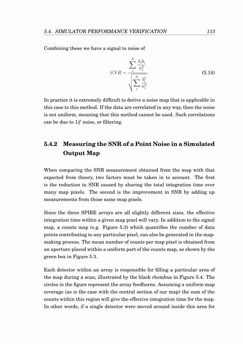
5.4. SIMULATOR PERFORMANCE VERIFICATION 113
Combining these we have a signal to noise of
SNR =
N∑i
Sibin2i√√√√ N∑
i
b2in2i
. (5.14)
In practice it is extremely difficult to derive a noise map that is applicable inthis case to this method. If the data are correlated in any way, then the noiseis not uniform, meaning that this method cannot be used. Such correlationscan be due to 1/f noise, or filtering.
5.4.2 Measuring the SNR of a Point Noise in a SimulatedOutput Map
When comparing the SNR measurement obtained from the map with thatexpected from theory, two factors must be taken in to account. The firstis the reduction in SNR caused by sharing the total integration time overmany map pixels. The second is the improvement in SNR by adding upmeasurements from those same map pixels.
Since the three SPIRE arrays are all slightly different sizes, the effectiveintegration time within a given map pixel will vary. In addition to the signalmap, a counts map (e.g. Figure 5.3) which quantifies the number of datapoints contributing to any particular pixel, can also be generated in the map-making process. The mean number of counts per map pixel is obtained froman aperture placed within a uniform part of the counts map, as shown by thegreen box in Figure 5.3.
Each detector within an array is responsible for filling a particular area ofthe map during a scan, illustrated by the black rhombus in Figure 5.4. Thecircles in the figure represent the array feedhorns. Assuming a uniform mapcoverage (as is the case with the central section of our map) the sum of thecounts within this region will give the effective integration time for the map.In other words, if a single detector were moved around inside this area for
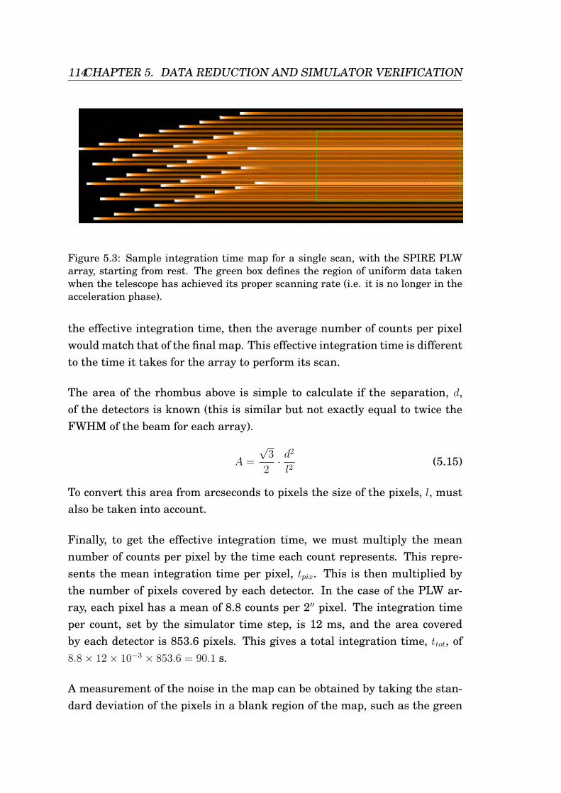
114CHAPTER 5. DATA REDUCTION AND SIMULATOR VERIFICATION
Figure 5.3: Sample integration time map for a single scan, with the SPIRE PLWarray, starting from rest. The green box defines the region of uniform data takenwhen the telescope has achieved its proper scanning rate (i.e. it is no longer in theacceleration phase).
the effective integration time, then the average number of counts per pixelwould match that of the final map. This effective integration time is differentto the time it takes for the array to perform its scan.
The area of the rhombus above is simple to calculate if the separation, d,of the detectors is known (this is similar but not exactly equal to twice theFWHM of the beam for each array).
A =
√3
2· d
2
l2(5.15)
To convert this area from arcseconds to pixels the size of the pixels, l, mustalso be taken into account.
Finally, to get the effective integration time, we must multiply the meannumber of counts per pixel by the time each count represents. This repre-sents the mean integration time per pixel, tpix. This is then multiplied bythe number of pixels covered by each detector. In the case of the PLW ar-ray, each pixel has a mean of 8.8 counts per 2′′ pixel. The integration timeper count, set by the simulator time step, is 12 ms, and the area coveredby each detector is 853.6 pixels. This gives a total integration time, ttot, of8.8× 12× 10−3 × 853.6 = 90.1 s.
A measurement of the noise in the map can be obtained by taking the stan-dard deviation of the pixels in a blank region of the map, such as the green
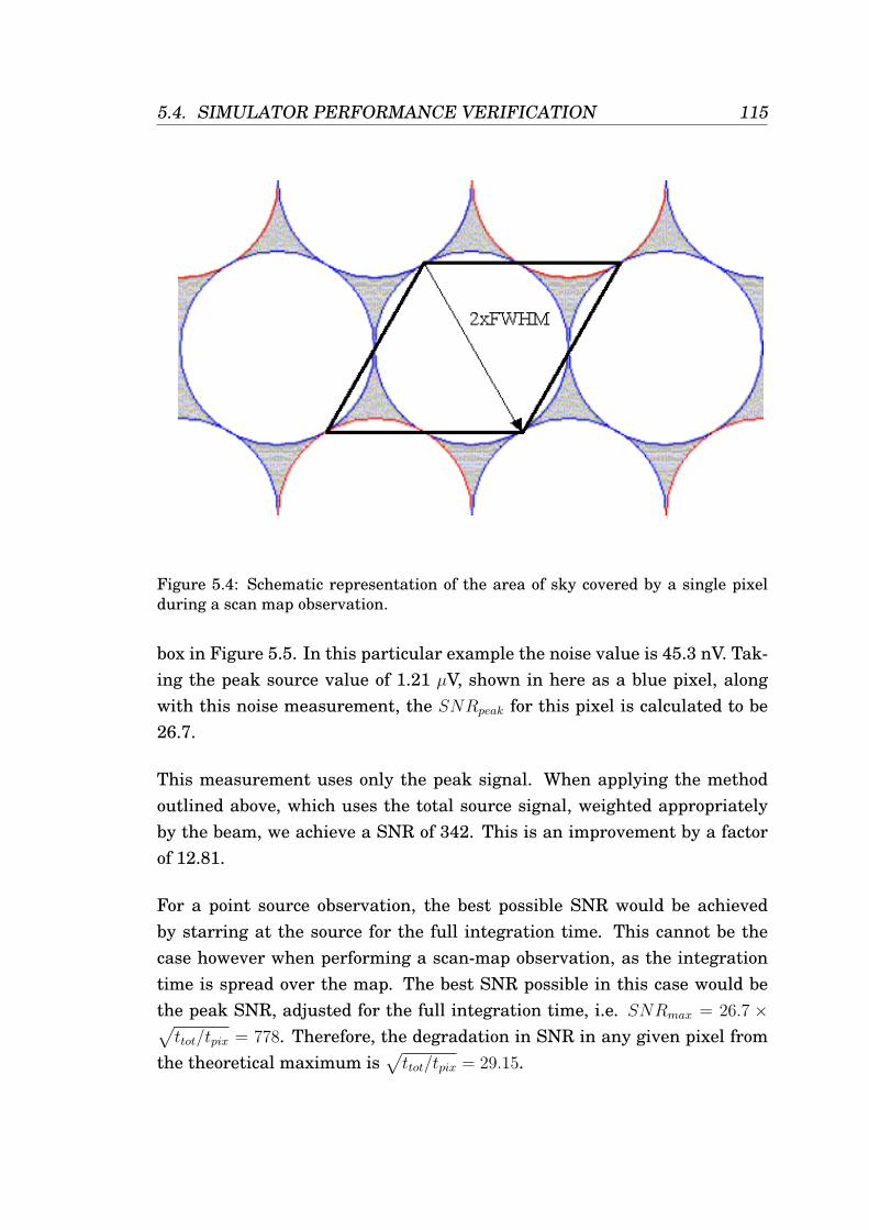
5.4. SIMULATOR PERFORMANCE VERIFICATION 115
Figure 5.4: Schematic representation of the area of sky covered by a single pixelduring a scan map observation.
box in Figure 5.5. In this particular example the noise value is 45.3 nV. Tak-ing the peak source value of 1.21 µV, shown in here as a blue pixel, alongwith this noise measurement, the SNRpeak for this pixel is calculated to be26.7.
This measurement uses only the peak signal. When applying the methodoutlined above, which uses the total source signal, weighted appropriatelyby the beam, we achieve a SNR of 342. This is an improvement by a factorof 12.81.
For a point source observation, the best possible SNR would be achievedby starring at the source for the full integration time. This cannot be thecase however when performing a scan-map observation, as the integrationtime is spread over the map. The best SNR possible in this case would bethe peak SNR, adjusted for the full integration time, i.e. SNRmax = 26.7 ×√ttot/tpix = 778. Therefore, the degradation in SNR in any given pixel from
the theoretical maximum is√ttot/tpix = 29.15.
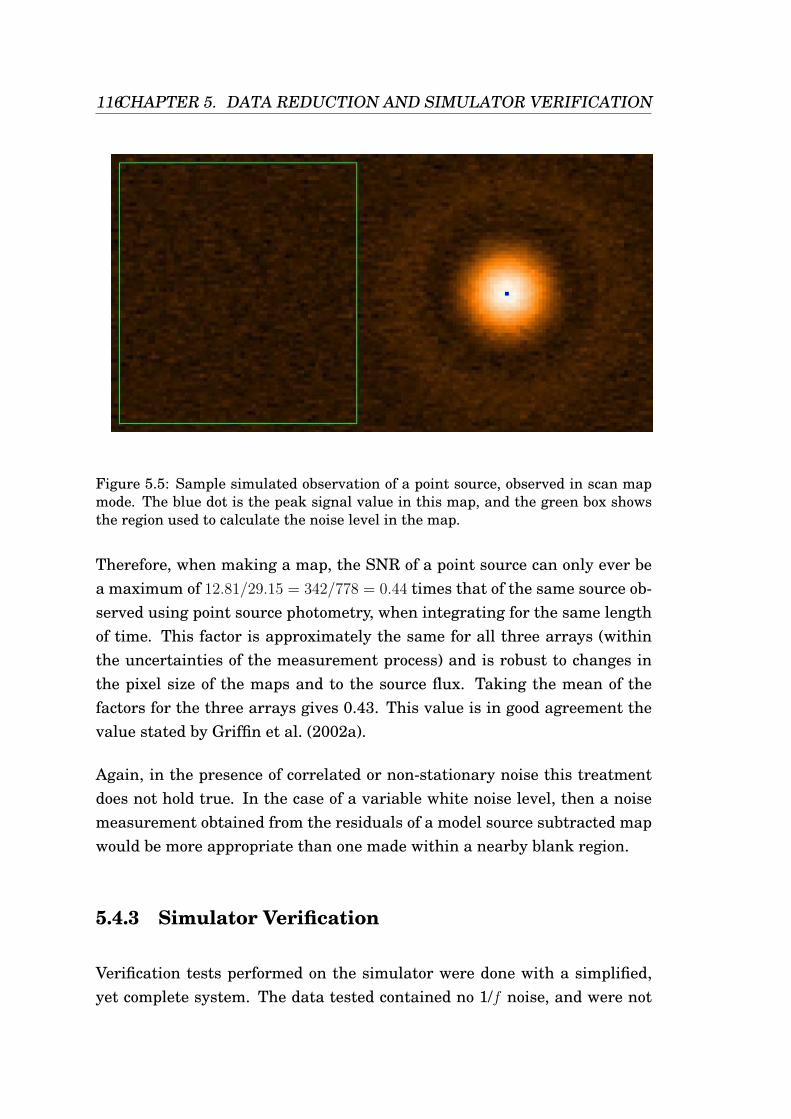
116CHAPTER 5. DATA REDUCTION AND SIMULATOR VERIFICATION
Figure 5.5: Sample simulated observation of a point source, observed in scan mapmode. The blue dot is the peak signal value in this map, and the green box showsthe region used to calculate the noise level in the map.
Therefore, when making a map, the SNR of a point source can only ever bea maximum of 12.81/29.15 = 342/778 = 0.44 times that of the same source ob-served using point source photometry, when integrating for the same lengthof time. This factor is approximately the same for all three arrays (withinthe uncertainties of the measurement process) and is robust to changes inthe pixel size of the maps and to the source flux. Taking the mean of thefactors for the three arrays gives 0.43. This value is in good agreement thevalue stated by Griffin et al. (2002a).
Again, in the presence of correlated or non-stationary noise this treatmentdoes not hold true. In the case of a variable white noise level, then a noisemeasurement obtained from the residuals of a model source subtracted mapwould be more appropriate than one made within a nearby blank region.
5.4.3 Simulator Verification
Verification tests performed on the simulator were done with a simplified,yet complete system. The data tested contained no 1/f noise, and were not
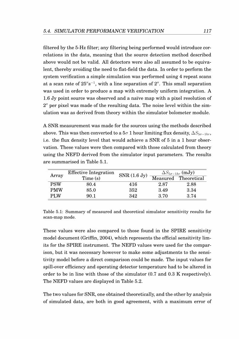
5.4. SIMULATOR PERFORMANCE VERIFICATION 117
filtered by the 5-Hz filter; any filtering being performed would introduce cor-relations in the data, meaning that the source detection method describedabove would not be valid. All detectors were also all assumed to be equiva-lent, thereby avoiding the need to flat-field the data. In order to perform thesystem verification a simple simulation was performed using 4 repeat scansat a scan rate of 25′′s−1, with a line separation of 2′′. This small separationwas used in order to produce a map with extremely uniform integration. A1.6 Jy point source was observed and a naıve map with a pixel resolution of2′′ per pixel was made of the resulting data. The noise level within the sim-ulation was as derived from theory within the simulator bolometer module.
A SNR measurement was made for the sources using the methods describedabove. This was then converted to a 5σ 1 hour limiting flux density, ∆S5σ−1hr,i.e. the flux density level that would achieve a SNR of 5 in a 1 hour obser-vation. These values were then compared with those calculated from theoryusing the NEFD derived from the simulator input parameters. The resultsare summarised in Table 5.1.
Array Effective Integration SNR (1.6 Jy) ∆S5σ−1hr (mJy)Time (s) Measured Theoretical
PSW 80.4 416 2.87 2.88PMW 85.0 352 3.49 3.34PLW 90.1 342 3.70 3.74
Table 5.1: Summary of measured and theoretical simulator sensitivity results forscan-map mode.
These values were also compared to those found in the SPIRE sensitivitymodel document (Griffin, 2004), which represents the official sensitivity lim-its for the SPIRE instrument. The NEFD values were used for the compar-ison, but it was necessary however to make some adjustments to the sensi-tivity model before a direct comparison could be made. The input values forspill-over efficiency and operating detector temperature had to be altered inorder to be in line with those of the simulator (0.7 and 0.3 K respectively).The NEFD values are displayed in Table 5.2.
The two values for SNR, one obtained theoretically, and the other by analysisof simulated data, are both in good agreement, with a maximum error of
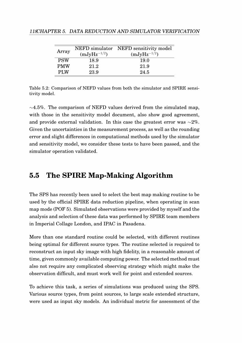
118CHAPTER 5. DATA REDUCTION AND SIMULATOR VERIFICATION
Array NEFD simulator NEFD sensitivity model(mJyHz−1/2) (mJyHz−1/2)
PSW 18.9 19.0PMW 21.2 21.9PLW 23.9 24.5
Table 5.2: Comparison of NEFD values from both the simulator and SPIRE sensi-tivity model.
∼4.5%. The comparison of NEFD values derived from the simulated map,with those in the sensitivity model document, also show good agreement,and provide external validation. In this case the greatest error was ∼2%.Given the uncertainties in the measurement process, as well as the roundingerror and slight differences in computational methods used by the simulatorand sensitivity model, we consider these tests to have been passed, and thesimulator operation validated.
5.5 The SPIRE Map-Making Algorithm
The SPS has recently been used to select the best map making routine to beused by the official SPIRE data reduction pipeline, when operating in scanmap mode (POF 5). Simulated observations were provided by myself and theanalysis and selection of these data was performed by SPIRE team membersin Imperial Collage London, and IPAC in Pasadena.
More than one standard routine could be selected, with different routinesbeing optimal for different source types. The routine selected is required toreconstruct an input sky image with high fidelity, in a reasonable amount oftime, given commonly available computing power. The selected method mustalso not require any complicated observing strategy which might make theobservation difficult, and must work well for point and extended sources.
To achieve this task, a series of simulations was produced using the SPS.Various source types, from point sources, to large scale extended structure,were used as input sky models. An individual metric for assessment of the
5.5. THE SPIRE MAP-MAKING ALGORITHM 119
performance of each science case was defined.
Two simulations of each input sky were performed using the nominal scanmap parameters (see Chapter 6). The two simulations were performed atdifferent scan angles to provide cross-linking. At the map-making stage itis assumed that the data have been cleaned, and contain no glitches, cor-related noise, or differences in detector response. Therefore the key issueto be tackled by these routines is uncorrelated 1/f noise individual to eachdetector.
Six map-making routines were compared. The first was a naıve mappingmethod, which was used as a reference. The second method again useda naıve mapping routine, but pre-filtered the data using Fourier methods.An adapted version of the Spitzer MOsaicking and Point source EXtraction(MOPEX) mapping routine was also used (Makovoz and Khan, 2005). Thisfiltered the data and constructed the map in a similar way to the previousmethod. The map making routine used for the BOLOCAM instrument onthe Caltech Submillimetre Observatory was used (Haig et al., 2004), whichworks by performing an iterative principle component analysis (PCA). Thefinal two methods attempt to produce a maximum likelihood map by solvingEquation 5.3. The first method, called Constrained Mapmaker (CM), uses aniterative approach (Crill and Netterfield, in prep.), while the second method,MADmap, solves the equation by making several assumptions about the sta-tionarity of the noise, i.e. the stability of the noise properties, and invertingthe covariance matrix directly (Christopher, 2002).
Different input maps were used to test each map-making algorithgm’s abil-ity to deal with various science cases. Figures 5.6–5.11 contain examples ofone particular input map case for each of the six mapping methods used. Thespecific example is the observation of a simple simulated input source withan exponential radial flux density profile. The exponential source is trun-cated at a particular radius resulting in the step seen in the figures. Some ofthe methods requiring filtering (Figures 5.8 and 5.9) show clear dark lobeseither side of the source in the scan direction, characteristic of this type ofmethod. A distortion in the source shape can also be seen with the MOPEXmethod (Figure 5.8). Clear striping can be seen in the naıve, filtered and
120CHAPTER 5. DATA REDUCTION AND SIMULATOR VERIFICATION
BOLOCAM methods (Figures 5.6, 5.7, and 5.9). Both of the maximum like-lihood map-making routines (Figures 5.10 and 5.11) perform well, with min-imal striping visible when cross-linking (cross scanning), required for thesemethods to operate optimally, is performed. When cross-linking is not per-formed, these methods are essentially reduced to a naıve map makers.
The finding of the selection board was that CM and MADmap were the twostrongest mapping routines in terms of data quality. The two forms of naıvemapping produce an intermediate result, and so were discounted. Whilethe BOLOCAM code does well with point sources, it is optimised for groundbased observations and does not do well at recovering extended emission.
MADmap was finally chosen over CM for the following reasons:
• it performs better than CM on extended sources;
• it is more robust (CM is still in the development stages);
• it is competitive with just a single iteration;
• it is relatively simple to incorporate into the current pipeline;
• as a maximum likelihood method, it has the scope for improved perfor-mance with increased cross-linking.
The full results of this investigation can be found in the official report byClements et al. (2006). It is intended that this work be published in the nearfuture.
5.6 Chapter Summary
This Chapter has outlined some of the major data processing tasks requiredto convert raw instrument timeline data into a useable format for astronomy,in this case a map. It highlights various data cleaning process, includingremoval of cosmic ray detections, correlated noise, and flat-fielding. Where
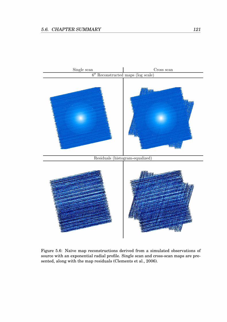
5.6. CHAPTER SUMMARY 121
Table 7: Large Exponential Disk – Direct (Naive) MappingSingle scan Cross scan
6′′ Reconstructed maps (log scale)
Residuals (histogram-equalized)
σ [mJy/pixel] 1.7027 1.3082Total flux ratio 1.0155 1.0097Mean profile ratio 1.0134 1.0082Std. Dev. profile ratio 0.0339 0.0204Execution time 33.1s 56.6s
39
Figure 5.6: Naıve map reconstructions derived from a simulated observations ofsource with an exponential radial profile. Single scan and cross-scan maps are pre-sented, along with the map residuals (Clements et al., 2006).
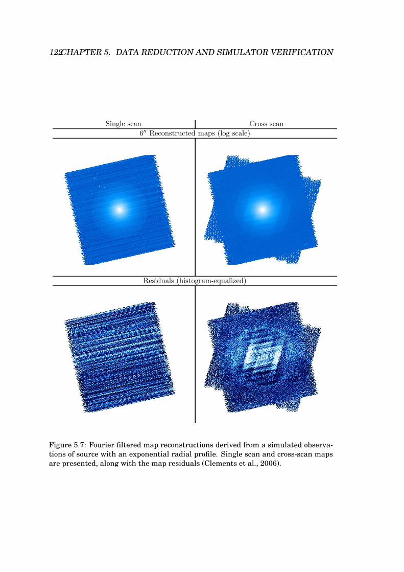
122CHAPTER 5. DATA REDUCTION AND SIMULATOR VERIFICATION
Table 31: Large Exponential Disk – Filtered MappingSingle scan Cross scan
6′′ Reconstructed maps (log scale)
Residuals (histogram-equalized)
σ [mJy/pixel] 1.7027 1.1988Total flux ratio 1.0155 1.0194Mean profile ratio 1.0134 0.9891Std. Dev. profile ratio 0.0339 0.0876Execution time 4m15s 4m56s
63
Figure 5.7: Fourier filtered map reconstructions derived from a simulated observa-tions of source with an exponential radial profile. Single scan and cross-scan mapsare presented, along with the map residuals (Clements et al., 2006).
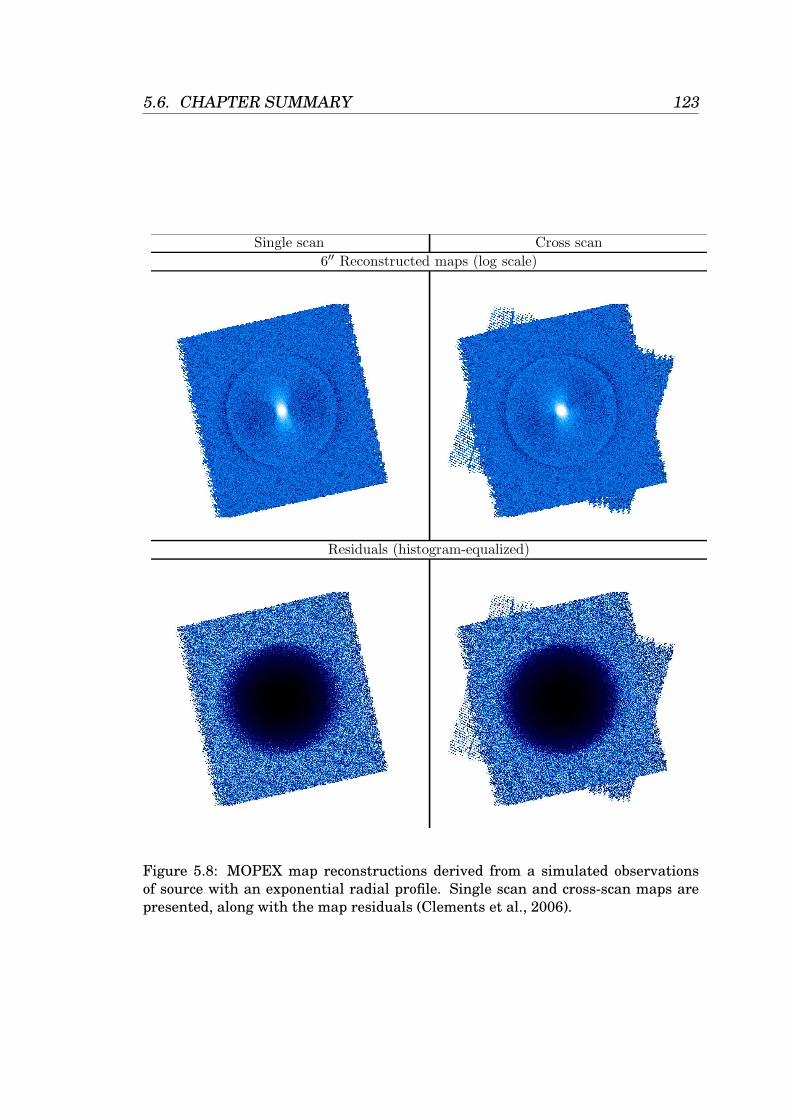
5.6. CHAPTER SUMMARY 123
Table 47: Large Exponential Disk – MOPEX with High Pass FilterSingle scan Cross scan
6′′ Reconstructed maps (log scale)
Residuals (histogram-equalized)
σ [mJy/pixel] 8.5428 8.5051Total flux ratio 0.0754 0.0736Mean profile ratio 0.1070 0.1067Std. Dev. profile ratio 0.1180 0.1147Execution time 3h39m29s 12h03m15s
79
Figure 5.8: MOPEX map reconstructions derived from a simulated observationsof source with an exponential radial profile. Single scan and cross-scan maps arepresented, along with the map residuals (Clements et al., 2006).
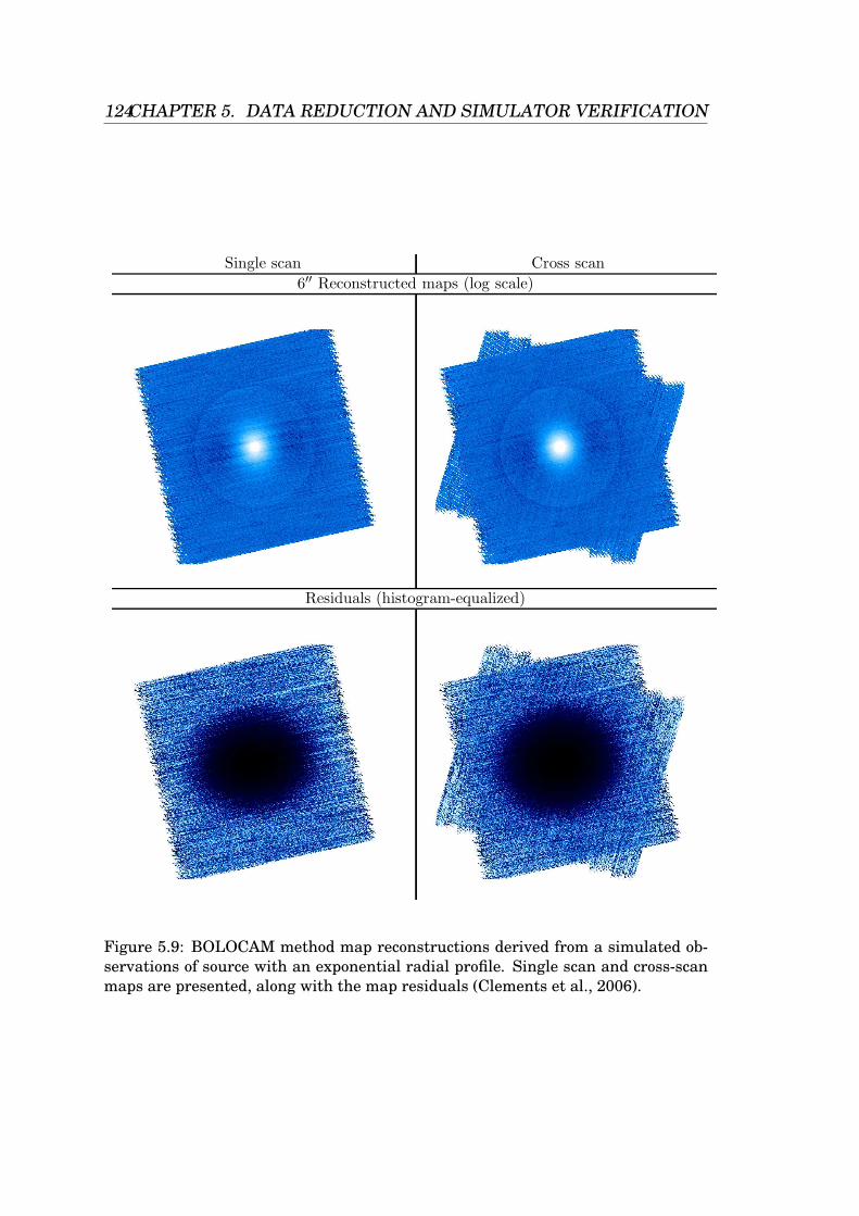
124CHAPTER 5. DATA REDUCTION AND SIMULATOR VERIFICATION
Table 55: Large Exponential Disk – BolocamSingle scan Cross scan
6′′ Reconstructed maps (log scale)
Residuals (histogram-equalized)
σ [mJy/pixel] 4.8942 5.2480Total flux ratio 0.3255 0.2745Mean profile ratio 0.3210 0.2793Std. Dev. profile ratio 0.1969 0.1990Execution time 7m40s 10m44s
87
Figure 5.9: BOLOCAM method map reconstructions derived from a simulated ob-servations of source with an exponential radial profile. Single scan and cross-scanmaps are presented, along with the map residuals (Clements et al., 2006).
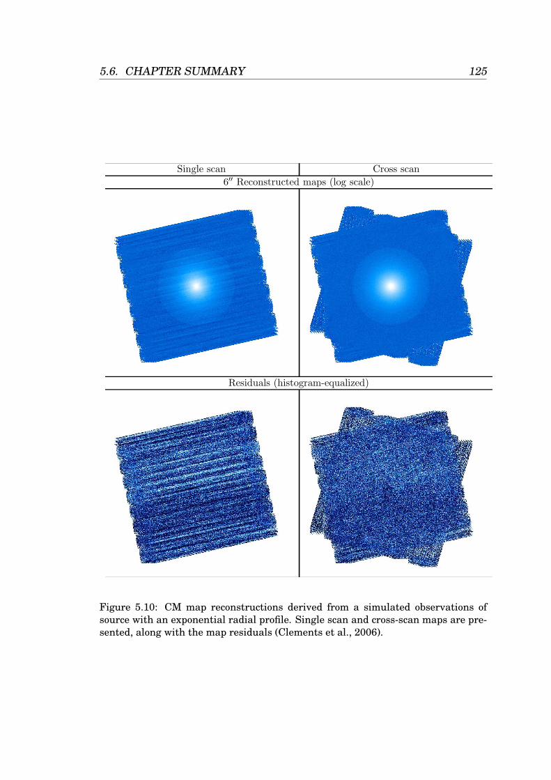
5.6. CHAPTER SUMMARY 125
Table 15: Large Exponential Disk – CMSingle scan Cross scan
6′′ Reconstructed maps (log scale)
Residuals (histogram-equalized)
σ [mJy/pixel] 1.8160 1.2887Total flux ratio 1.0074 1.0019Mean profile ratio 1.0099 1.0037Std. Dev. profile ratio 0.0337 0.0158Execution time 1m54s 2m48s
47
Figure 5.10: CM map reconstructions derived from a simulated observations ofsource with an exponential radial profile. Single scan and cross-scan maps are pre-sented, along with the map residuals (Clements et al., 2006).
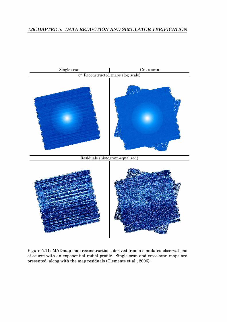
126CHAPTER 5. DATA REDUCTION AND SIMULATOR VERIFICATION
Table 23: Large Exponential Disk – MADmap (Ncorr=200)Single scan Cross scan
6′′ Reconstructed maps (log scale)
Residuals (histogram-equalized)
σ [mJy/pixel] 1.2005 0.7526Total flux ratio 1.0141 1.0072Mean profile ratio 1.0120 1.0090Std. Dev. profile ratio 0.0341 0.0145Execution time 42.6s 1m02s
55
Figure 5.11: MADmap map reconstructions derived from a simulated observationsof source with an exponential radial profile. Single scan and cross-scan maps arepresented, along with the map residuals (Clements et al., 2006).
5.6. CHAPTER SUMMARY 127
necessary, an explanation of these methods, as applied to SPS data, was alsogiven.
The issues involved with making maps from the processed data were dis-cussed, including an explanation of naıve map making, and an overview ofthe maximum likelihood map-making method. This method deals with theremoval of uncorrelated 1/f noise, and is used widely in studies of the CMB.
An account of the validation of the SPS signal and noise output was thenpresented. This validation was performed by comparing the SNR of a pointsource, observed in scan-map mode, with the theoretical SNR expected. Thisused data in the form of a naıve map, generated by unfiltered detector data.The NEFD obtained in this verification exercise was compared to the officialSPIRE sensitivity model (Griffin, 2004), and found to agree to within ∼ 2%.
Finally, an overview of the SPIRE map-making routine selection process waspresented, and the reasons for selecting MADmap as the best routine ex-plained.

128CHAPTER 5. DATA REDUCTION AND SIMULATOR VERIFICATION
Chapter 6
Observing Mode Optimisation
With the overall cost of Herschel being approximately e1 million per day,the efficient use of observing time is essential. Therefore, the optimisationof the photometer observing modes, outlined in Section 3.2, is an essentialpart of the SPIRE pre-flight planning. Not only must the modes be efficient,they must also return a high quality of data. Since a significant fractionof the SPIRE observing time will be in the form of large scale photometricsurvey programmes, it is particularly important that the scan-map mode becarefully optimised in terms of efficiency and data quality.
This chapter describes the use of the simulator in the optimisation of theSPIRE photometer observatory functions. The key parameters for each ob-serving mode are described, and the use of the SPS in the determinationtheir optimal value is presented.
6.1 Point Source Photometry
The parameters available for optimisation within the point source photom-etry observing modes are chop frequency, fchop, chop throw, ∆chop, chop di-rection, nod frequency, fnod, and nod throw. Most of these parameters areactually fixed or constrained by the design of the instrument. For example
129
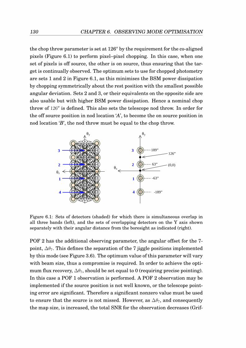
130 CHAPTER 6. OBSERVING MODE OPTIMISATION
the chop throw parameter is set at 126′′ by the requirement for the co-alignedpixels (Figure 6.1) to perform pixel–pixel chopping. In this case, when oneset of pixels is off source, the other is on source, thus ensuring that the tar-get is continually observed. The optimum sets to use for chopped photometryare sets 1 and 2 in Figure 6.1, as this minimises the BSM power dissipationby chopping symmetrically about the rest position with the smallest possibleangular deviation. Sets 2 and 3, or their equivalents on the opposite side arealso usable but with higher BSM power dissipation. Hence a nominal chopthrow of 126′′ is defined. This also sets the telescope nod throw. In order forthe off source position in nod location ‘A’, to become the on source position innod location ‘B’, the nod throw must be equal to the chop throw.
Ref: SPIRE-RAL-DOC-000320
Issue: 3.3 Date: June 24 2005 Page: 19 of 19
Project Document
SPIRE Operating Modes for the SPIRE Instrument
3.1.1 POF 1: Chop Without Jiggling
Purpose: This is similar to what is often done on ground-based submillimetre telescopes. It is designed to make observations of a point or compact source of accurately known position. In the case of SPIRE, chopping between pairs of pixels gives maximum sensitivity because in that case the source is being observed all the time. There is simultaneous overlap at all three wavelengths for several sets of detectors on the SPIRE arrays. The optimum sets to use for chopped photometry are sets 1 and 2 in Figure 3.1 as this minimises the BSM power dissipation by chopping symmetrically about the rest position with the smallest possible angular deviation. Sets 2 and 3, or their equivalents on the opposite side are also usable but with higher BSM dissipation.
Figure 3.1: Left: sets of detectors (shaded) for which there is simultaneous overlap in all three bands for the feedhorn array option. Right: the sets of overlapping detectors on the Y axis shown separately with their angular distance from the boresight as indicated.
Description: 1. This Observatory Function is composed of the following instrument and Spacecraft Functions:
Instrument Function: Photometer Chop Spacecraft Function: Nod
2. Chop distance on the array: This is determined by the horn centre-centre spacing, and is equal to twice the 5-mm outside diameter of the PLW horn. The chop angle on the sky is equal to the distance moved in the focal plane multiplied by the plate scale (12.6 “/mm): Chop distance in the array focal plane: ∆ychop = 2 x 5 mm = 10 mm Chop angle on the sky: ∆θchop = (10 mm)(12.6 "/mm) = 126 arcsec. This mode requires pointing accuracy sufficiently good that the loss of signal due to the pointing error is acceptable. The signal loss factors for the photometer beams are shown in Figure 3.2 The required APE (3.7") corresponds to (11%, 6%, 3%) signal loss in the PLW, PMW and PSW bands mm respectively. The goal (1.5") corresponds to (2%, 1%, 0.5%) signal loss. For most observations, 11% is not acceptable, but 2% is. Therefore, the required APE is not good enough to allow accurate photometry at 250 mm without peaking up, but the goal is sufficient to allow this. In the event that the
3
1
θy
θz
2
4
3
1
θy
2
4
189”
-189”
-63”
63” θz
(0,0)
126”
Figure 6.1: Sets of detectors (shaded) for which there is simultaneous overlap inall three bands (left), and the sets of overlapping detectors on the Y axis shownseparately with their angular distance from the boresight as indicated (right).
POF 2 has the additional observing parameter, the angular offset for the 7-point, ∆θ7. This defines the separation of the 7 jiggle positions implementedby this mode (see Figure 3.6). The optimum value of this parameter will varywith beam size, thus a compromise is required. In order to achieve the opti-mum flux recovery, ∆θ7, should be set equal to 0 (requiring precise pointing).In this case a POF 1 observation is performed. A POF 2 observation may beimplemented if the source position is not well known, or the telescope point-ing error are significant. Therefore a significant nonzero value must be usedto ensure that the source is not missed. However, as ∆θ7, and consequentlythe map size, is increased, the total SNR for the observation decreases (Grif-

6.2. FIELD MAPPING 131
fin et al., 2002a), decreasing the accuracy of the measurement. Converselyas the map size increases, the contrast between the map positions increases,thereby allowing a more accurate measurement of the source position. Thisoccurs up until a point, beyond which the decrease in overall SNR outweighsthis improvement.
A series of simulations was performed to evaluate the recovery of the peakflux and position of a point source, as a function of ∆θ7. A symmetric Gaus-sian telescope beam was assumed in this case. The error on the measure-ment of these data was assessed as a function of ∆θ7 and pointing error, ∆.Simulations were performed for sources with a worst case SNR = 3, and anideal case SNR = 10 (Figure 6.2).
An optimum value for ∆θ7 of 0.3 beam FWHM was derived (Sibthorpe et al.,2005), corresponding to ∼5, 7, and 10′′ for the PSW, PMW, and PLW bandsrespectively. The PSW value works well for all bands, despite the variationin beams, as a high pointing error is still relatively small as a fraction of thelarger beam sizes. This also allows the longer wavelength bands to benefitfrom the advantages seen when using a smaller map, i.e. better peak fluxrecovery. For a modest SNR of ∼10, and pointing error of ∼0.2-0.3 PSWbeam FWHM, a typical peak flux error of ∼7 %, and positional error of ∼7 %
of the beam FWHM can be expected.
Herschel has an absolute pointing error requirement of 3.7′′(although a valueof 2′′ is expected to be achieved). The SPIRE team has decided that 7-pointphotometry (POF 2) will be adopted as the standard observing mode for pointsources, with a nominal separation of 6′′. This will ensure a good fit to bothsource position and flux.
6.2 Field Mapping
A POF 3 (jiggle map) observation is constructed from a series of independentPOF 1 (point source photometry) observations. As a result, many of therelevant optimum parameter values are as for POF 1. In this case however,
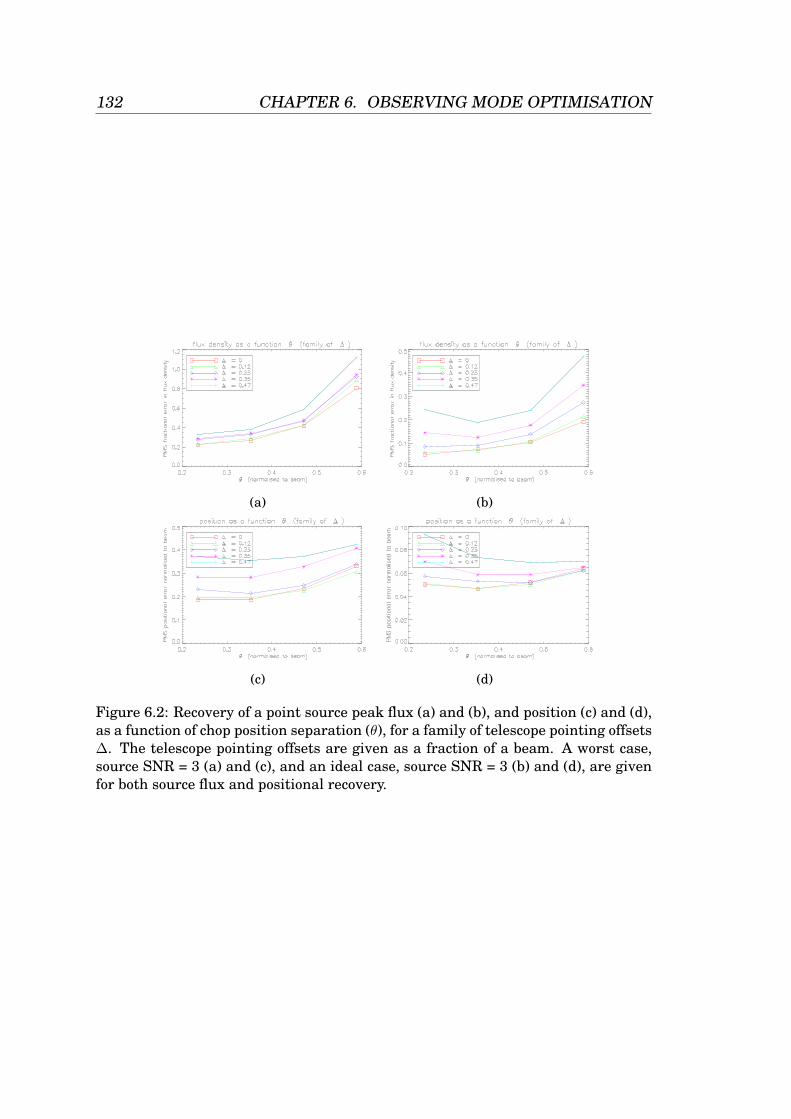
132 CHAPTER 6. OBSERVING MODE OPTIMISATION
(a) (b)
(c) (d)
Figure 6.2: Recovery of a point source peak flux (a) and (b), and position (c) and (d),as a function of chop position separation (θ), for a family of telescope pointing offsets∆. The telescope pointing offsets are given as a fraction of a beam. A worst case,source SNR = 3 (a) and (c), and an ideal case, source SNR = 3 (b) and (d), are givenfor both source flux and positional recovery.
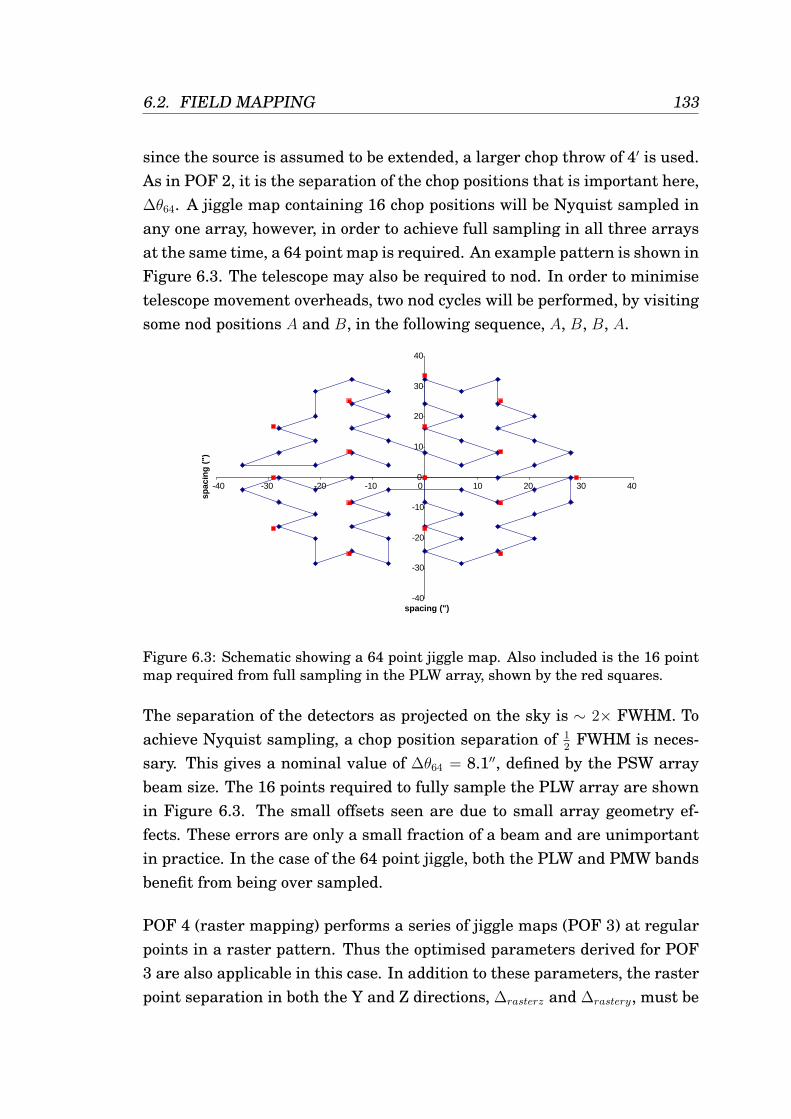
6.2. FIELD MAPPING 133
since the source is assumed to be extended, a larger chop throw of 4′ is used.As in POF 2, it is the separation of the chop positions that is important here,∆θ64. A jiggle map containing 16 chop positions will be Nyquist sampled inany one array, however, in order to achieve full sampling in all three arraysat the same time, a 64 point map is required. An example pattern is shown inFigure 6.3. The telescope may also be required to nod. In order to minimisetelescope movement overheads, two nod cycles will be performed, by visitingsome nod positions A and B, in the following sequence, A, B, B, A.
-40
-30
-20
-10
0
10
20
30
40
-40 -30 -20 -10 0 10 20 30 40
spacing (")
spac
ing
(")
Figure 6.3: Schematic showing a 64 point jiggle map. Also included is the 16 pointmap required from full sampling in the PLW array, shown by the red squares.
The separation of the detectors as projected on the sky is ∼ 2× FWHM. Toachieve Nyquist sampling, a chop position separation of 1
2FWHM is neces-
sary. This gives a nominal value of ∆θ64 = 8.1′′, defined by the PSW arraybeam size. The 16 points required to fully sample the PLW array are shownin Figure 6.3. The small offsets seen are due to small array geometry ef-fects. These errors are only a small fraction of a beam and are unimportantin practice. In the case of the 64 point jiggle, both the PLW and PMW bandsbenefit from being over sampled.
POF 4 (raster mapping) performs a series of jiggle maps (POF 3) at regularpoints in a raster pattern. Thus the optimised parameters derived for POF3 are also applicable in this case. In addition to these parameters, the rasterpoint separation in both the Y and Z directions, ∆rasterz and ∆rastery, must be
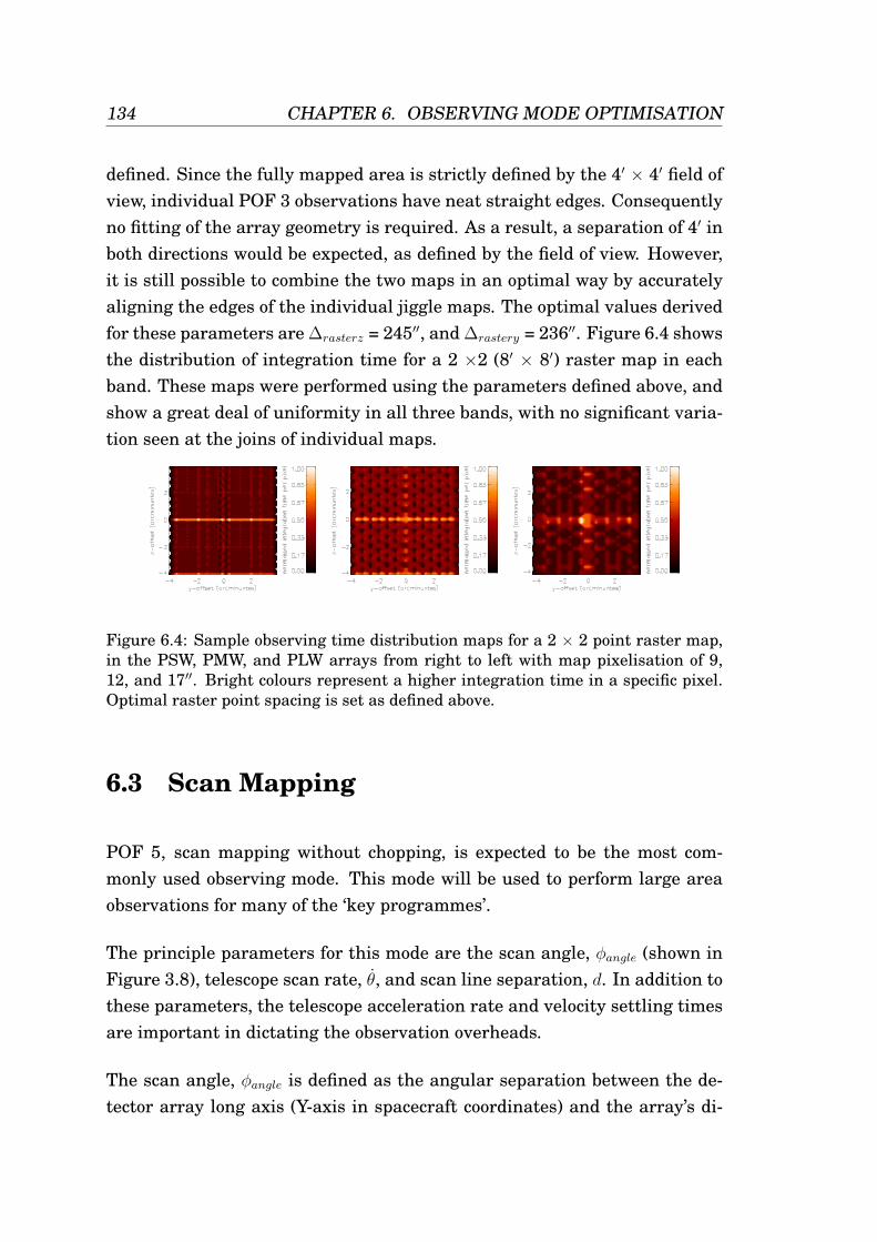
134 CHAPTER 6. OBSERVING MODE OPTIMISATION
defined. Since the fully mapped area is strictly defined by the 4′ × 4′ field ofview, individual POF 3 observations have neat straight edges. Consequentlyno fitting of the array geometry is required. As a result, a separation of 4′ inboth directions would be expected, as defined by the field of view. However,it is still possible to combine the two maps in an optimal way by accuratelyaligning the edges of the individual jiggle maps. The optimal values derivedfor these parameters are ∆rasterz = 245′′, and ∆rastery = 236′′. Figure 6.4 showsthe distribution of integration time for a 2 ×2 (8′ × 8′) raster map in eachband. These maps were performed using the parameters defined above, andshow a great deal of uniformity in all three bands, with no significant varia-tion seen at the joins of individual maps.
Figure 6.4: Sample observing time distribution maps for a 2 × 2 point raster map,in the PSW, PMW, and PLW arrays from right to left with map pixelisation of 9,12, and 17′′. Bright colours represent a higher integration time in a specific pixel.Optimal raster point spacing is set as defined above.
6.3 Scan Mapping
POF 5, scan mapping without chopping, is expected to be the most com-monly used observing mode. This mode will be used to perform large areaobservations for many of the ‘key programmes’.
The principle parameters for this mode are the scan angle, φangle (shown inFigure 3.8), telescope scan rate, θ, and scan line separation, d. In addition tothese parameters, the telescope acceleration rate and velocity settling timesare important in dictating the observation overheads.
The scan angle, φangle is defined as the angular separation between the de-tector array long axis (Y-axis in spacecraft coordinates) and the array’s di-
6.3. SCAN MAPPING 135
rection of motion (Figure 3.8). Since the array is hexagonal packed it hassix-fold symmetry. Therefore, for every scan angle there are 2 other an-gles which can produce the same result, with each angle having an oppositecounterpart. These angles are illustrated in Figure 6.5. The three differentoptions are referred to as scanning in the long, short, and diagonal direc-tions, where ‘long’ refers to scanning along the long axis of the array, ‘short’refers to scanning along the short axis of the array, and ‘diagonal’ refers toscanning angle the intermediate angle of the array.
Traditionally instruments containing a hexagonally packed geometry detec-tor array would scan at the Nyquist angle (13.9) (Holland et al., 1999). Thisprovides Nyquist sampling but does not represent the highest spatial sam-pling achievable with the SPIRE arrays. Due to the relatively high numberof detectors within the SPIRE arrays it is possible to rely on trailing de-tectors to follow up on earlier detectors. In order to achieve higher spatialsampling, an angle was taken which ensures that a detector, as far as ispossible, does not pass directly over another detector’s central, or half widthhalf maximum position, until a substantial fraction of an array distance hasbeen travelled.
An optimum angle of 12.4 has been found which provides scan data suffi-cient to produce maps with 1
4FWHM sized map pixels (i.e. double Nyquist
sampling) in all three bands when scanning in the long direction. This pixelsize chosen is independent of beam size, but the choice of a pixel size greaterthan 1
2a beam would result in a degradation of spatial information within
the data. The high spatial sampling at 12.4 results in a high degree of uni-formity in the map’s signal to noise coverage (Figure 6.6(a)). Such uniformitywill be particularly important for the large-scale deep survey programs. Thisincreased uniformity is gained at the expense of some redundancy. However,redundancy is present in each scan with several strips of sky being visitedby more than one detector (albeit fewer strips than when scanning at theNyquist angle).
Gaps (map pixels containing no data) do appear in the PLW maps for scansin the diagonal and short directions, and also for the PMW array when scan-ning close to the short axis, as there are insufficient detectors in this di-
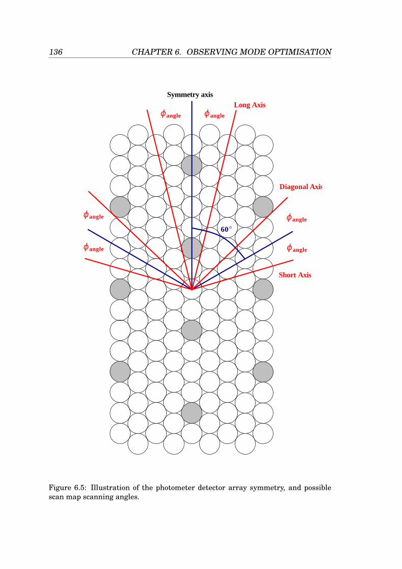
136 CHAPTER 6. OBSERVING MODE OPTIMISATION
φangle
Symmetry axis Long Axis
60°
φangle
φangle
φangle
φangle
φangle
Diagonal Axis
Short Axis
Figure 6.5: Illustration of the photometer detector array symmetry, and possiblescan map scanning angles.
6.3. SCAN MAPPING 137
rection to perform a fully sampled observation. In these cases, the doubleNyquist sampling (1/4 beam spacing) cannot be maintained. Using largerpixels alleviates this problem, and the sampling is still at least as good asin the Nyquist sampled case and are often better, i.e. pixel sizes remain ≤ 1
2
FWHM. Full sampling, meaning that there are no gaps in the maps for achosen pixel size, for the PLW array is achieved with pixel size of 14′′ fordiagonal and short scanning; full sampling for the PMW array is achievedwith a pixel size of 9′′ for short axis scanning. The main disadvantage of thisstrategy is lower redundancy – that is, fewer points of the sky are visited bymore than one pixel in a single scan leg.
In this analysis we have assumed 100% detector yield. While at present thenumber of dead detectors is very low (∼5%); this may not be the case once inflight. Dead detectors could lead to gaps in the maps, but scanning close tothe long axis will reduce this problem since there are more trailing detectorsto fill in the gaps. Therefore, it is recommended that the nominal scanningdirection be along the long axis. A disadvantage to this strategy however ishigher overhead time required during telescope turnaround, because the ar-ray has to travel further before the entire array has passed over the requiredmap area. For large maps this will be a minor fraction, but for smaller mapsit may be better to scan close to the short axis. Dithering of repeated mapscan then be used to fill in any holes within the map if necessary.
Since the PSW array is always fully sampled, with 14
beam FWHM pixels,when scanning at 12.4, even for diagonal and short axis scanning, the needfor larger than 1
4FWHM pixels in the other two arrays can in some cases
be offset. For example, source extraction can still be performed on the PSWarray using the smaller pixels with the associated higher spatial sampling.This will support the source extraction in the other two bands by giving animproved source position. If it is necessary to scan along either the diagonalor short axes (due to scheduling constraints or cross-linking requirements)then this angle still provides a good compromise between uniformity andredundancy. In any case, Nyquist scanning requires larger map pixels thandouble Nyquist scanning in all situations. Therefore, a scanning angle of12.4 is recommended, regardless of which axis the scanning direction isclosest to.
138 CHAPTER 6. OBSERVING MODE OPTIMISATION
For large square maps it is generally recommended that scans be made inthe diagonal direction. Using the two counterpart diagonal options, it is pos-sible to perform two almost orthogonal (∼95.2) scans maps. This providesa great deal of cross-linking in the data, providing redundancy and moreimportantly, the ability to implement the maximum likelihood map-makingroutines outlined in Section 5.3. The choice of these angles means that anequal amount of integration time is spent on each map section within a sin-gle scan. Scanning along the short, and then long axis, would produce a mapwith greater integration in time, per map area, being performed in short axisscan, than the long axis scan. The same integration time could be achievedin two scans along the long axis, but this would require scheduling the ob-servations months apart in order for the telescope orbit to rotate the arrayand make the observations possible. This is not necessary for the diagonalscan option.
Small (> 10′), or irregularly shaped maps, e.g. scans of long thin structures,will not benefit much from scanning with these two angles. This is becausethe overheads required to repoint the telescope may be greater than the timeto perform a single scan map. Here, the cross scan may not be more efficientthan simply performing another scan in the same direction. In this case, theobservation would scan along the long axis, thus recovering the 1
4FWHM
pixel size performance in all bands. The use of the cross scan is also notbeneficial for long thin maps, as they would only cross at one small point.Again, repeat maps in the same direction would be more efficient.
The optimum angular line separation, d, is the distance between successivescan lines that ensures the map is uniform in terms of distribution of inte-gration time, both along, and perpendicular to, the scan line direction. Inorder to achieve this, it is necessary to derive a separation which will alloweach scan line to fit perfectly into place with the previous line’s observation,thereby creating a scan equivalent to one made with a single array with aneffective size of n scan lines (Figure 6.6(b)).
This optimum scan separation depends on the particular array geometry,and hence is slightly different for each array. The optimum value of d for a
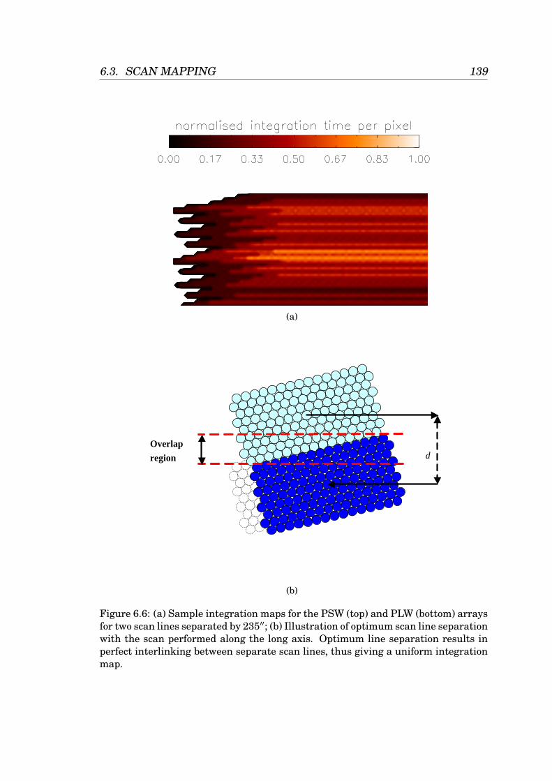
6.3. SCAN MAPPING 139
(a)
d Overlap region
(b)
Figure 6.6: (a) Sample integration maps for the PSW (top) and PLW (bottom) arraysfor two scan lines separated by 235′′; (b) Illustration of optimum scan line separationwith the scan performed along the long axis. Optimum line separation results inperfect interlinking between separate scan lines, thus giving a uniform integrationmap.
140 CHAPTER 6. OBSERVING MODE OPTIMISATION
given scan angle, scanning along the short axis, is given by Equation 6.1,
d =S
2(N√
3 cos(φscan)− sin(φscan)), (6.1)
where S is the bolometer separation on the sky in arcseconds (SPSW = 31.4,SPMW = 41.8, SPLW = 62.8), N is the number of bolometer rows making upeach array (NPSW = 9, NPMW = 7, NPLW = 5), and φscan is the scan angle. Fora scan angle of 12.4 the resultant values of d are 235, 243, and 258′′ for thePSW, PMW, and PLW bands respectively. In order to ensure fully sampledmaps in all bands an optimum separation of 235′′, corresponding to the PSWoptimum, has been chosen. This does result in some loss in uniformity in thePMW and PLW, where the integration time is slightly higher in the overlapregion, however this is more favorable than having unobserved regions inthe PSW maps. The equivalent optimum scan line separations when scan-ning in the diagonal and short directions are 348′′ and 455′′ respectively.
In addition to the slightly sub-optimal spacing in the PMW and PLW, therealso exists a small non-uniformity due to the variation in the make up ofthe different arrays. The pixels found at the corners of the PMW and PLWarrays do not have counterparts in the PSW. Consequently there is a slightincrease in integration time near the overlap, where there is an increase inthe total number of detectors observing a single line. This can be seen inFigure 6.6(a).
Optimisation of the scan rate parameter depends on two instrument system-atics: 1/f noise, defined by the knee frequency, and the on-board low-passfilter. The losses resulting from these systematics vary contrary to one an-other. As a result there is an optimum scan rate such that the net losses areminimised. A high scan rate reduces the effect of 1/f noise, and a slow ratereduces the losses and beam smearing due to the filter.
A series of simulations was performed in order to assess the impact of 1/f
noise on our ability to recover a point source during a single scan observa-tion. This impact was quantified by comparison of the output SNR with anidentical observation, performed with only white noise (Equation 6.2). This
6.4. OBSERVING MODE SELECTION 141
is referred to as the SNR loss factor, SNRloss.
SNRloss =SNRobs
SNRwhite
, (6.2)
where SNRobs is the output observation SNR, and SNRwhite is the SNR forthe same observation with white noise only. No attempts to remove the 1/f
noise were performed. A SNRloss value of unity would be the ideal case, i.e.no loss due to 1/f noise.
Since the optimum scan rate will vary with convolved source size scale, amore general parameter to use is the beam crossing time τ . This parametervaries as a function of the convolved source size scale and the scan rate. Theresults from the simulations performed are thus plotted as a function of τ(Figure 6.7), with the nominal SPIRE 1/f noise knee frequency of 100 mHz.The maximum value of the SNRloss, shown as the solid line in Figure 6.7(a),give the beam crossing time for which the systematic losses are minimised.Using this value Figure 6.7(b) was derived, giving the systematic losses as afunction of scan rate for each band. The optimum scan rate, chosen such thetotal losses across all three bands are minimised (i.e. the maximum valueof SNR loss factor), was found to be ∼30′′s−1. This value has been adoptedas the baseline value for SPIRE scan-map observations. Note however thatthe maximum scan rate of 60′′s−1 is useable with very little degradation inperformance, but will result in greater telescope overheads.
POF 6, scanning with chopping, is an auxiliary mode. If the 1/f noise inorbit is significantly greater than the nominal value, then this mode may beimplemented.
This parameterisation of 1/f noise loss is extended and used in further in-vestigations in Chapter 8.
6.4 Observing Mode Selection
A comparison of the efficiency of the raster and scan map modes was carriedout. The basic jiggle map figure of merit, against which scan map observa-
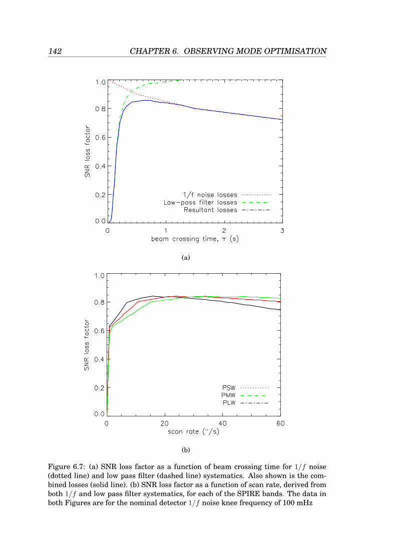
142 CHAPTER 6. OBSERVING MODE OPTIMISATION
(a)
(b)
Figure 6.7: (a) SNR loss factor as a function of beam crossing time for 1/f noise(dotted line) and low pass filter (dashed line) systematics. Also shown is the com-bined losses (solid line). (b) SNR loss factor as a function of scan rate, derived fromboth 1/f and low pass filter systematics, for each of the SPIRE bands. The data inboth Figures are for the nominal detector 1/f noise knee frequency of 100 mHz
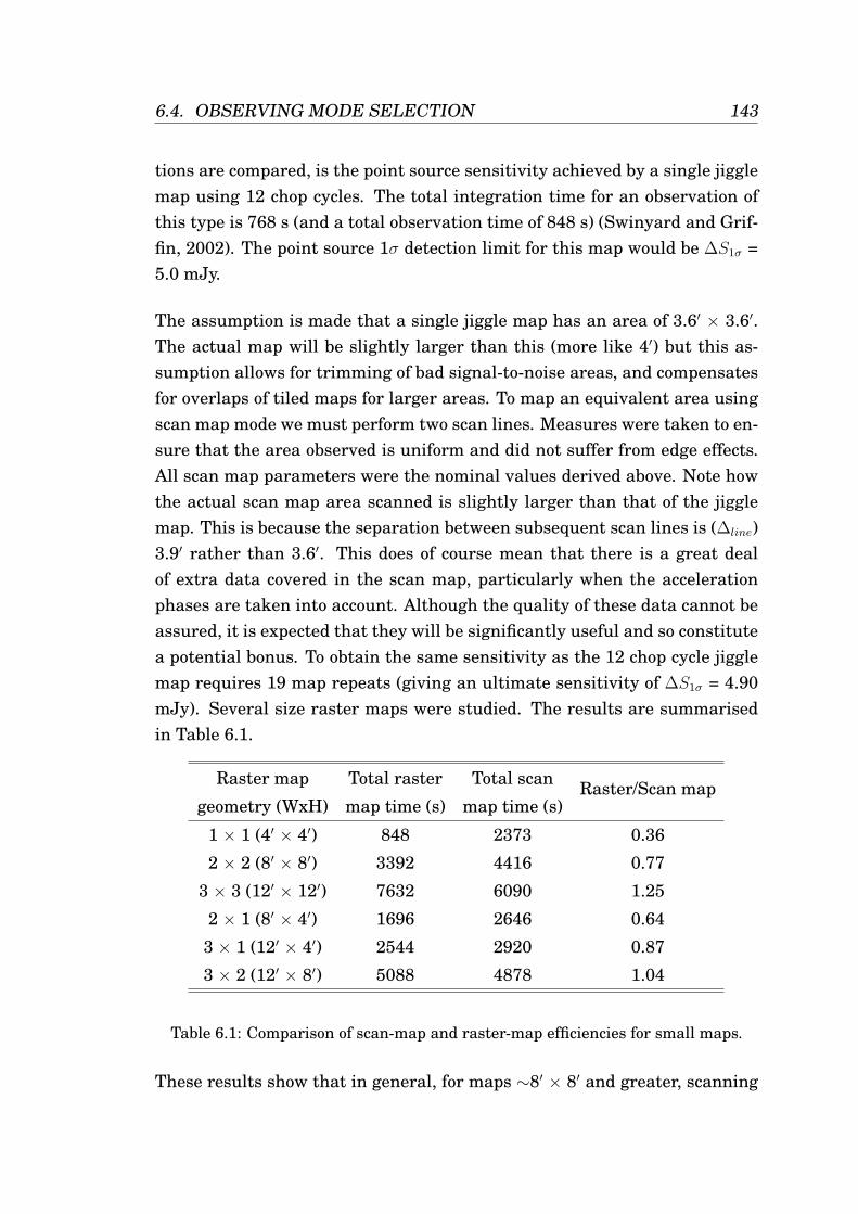
6.4. OBSERVING MODE SELECTION 143
tions are compared, is the point source sensitivity achieved by a single jigglemap using 12 chop cycles. The total integration time for an observation ofthis type is 768 s (and a total observation time of 848 s) (Swinyard and Grif-fin, 2002). The point source 1σ detection limit for this map would be ∆S1σ =5.0 mJy.
The assumption is made that a single jiggle map has an area of 3.6′ × 3.6′.The actual map will be slightly larger than this (more like 4′) but this as-sumption allows for trimming of bad signal-to-noise areas, and compensatesfor overlaps of tiled maps for larger areas. To map an equivalent area usingscan map mode we must perform two scan lines. Measures were taken to en-sure that the area observed is uniform and did not suffer from edge effects.All scan map parameters were the nominal values derived above. Note howthe actual scan map area scanned is slightly larger than that of the jigglemap. This is because the separation between subsequent scan lines is (∆line)3.9′ rather than 3.6′. This does of course mean that there is a great dealof extra data covered in the scan map, particularly when the accelerationphases are taken into account. Although the quality of these data cannot beassured, it is expected that they will be significantly useful and so constitutea potential bonus. To obtain the same sensitivity as the 12 chop cycle jigglemap requires 19 map repeats (giving an ultimate sensitivity of ∆S1σ = 4.90mJy). Several size raster maps were studied. The results are summarisedin Table 6.1.
Raster map Total raster Total scan Raster/Scan mapgeometry (WxH) map time (s) map time (s)
1 × 1 (4′ × 4′) 848 2373 0.36
2 × 2 (8′ × 8′) 3392 4416 0.77
3 × 3 (12′ × 12′) 7632 6090 1.25
2 × 1 (8′ × 4′) 1696 2646 0.64
3 × 1 (12′ × 4′) 2544 2920 0.87
3 × 2 (12′ × 8′) 5088 4878 1.04
Table 6.1: Comparison of scan-map and raster-map efficiencies for small maps.
These results show that in general, for maps ∼8′ × 8′ and greater, scanning
144 CHAPTER 6. OBSERVING MODE OPTIMISATION
is more efficient then jiggling. For this reason scan map mode is preferredfor all maps except a single 4′× 4′ field. This is because the majority of thescan map overheads are composed of the acceleration and deceleration at thebeginning and end of each scan line. The scan map efficiency is in generalhigher as it has a field of view twice that of the raster map. These overheadsare dependant on scan rate and not map size. Thus for large maps, scan mapwill always be more efficient.
Several other factors need to be taken into consideration if simple observingefficiency is not the primary concern. Because it involves chopping, rastermapping is immune to 1/f noise so this may be attractive in some cases.However, it also removes large scale structure, in which case scanning maybe preferable. The additional data around the edges of a small scan mapmay be useful albeit of lower quality than the main map area.
Since this analysis was carried out, the telescope movement overheads havebeen increased. The impact of this change on the results of the jiggle mapverses scan map study is currently under investigation. The situation re-garding the final telescope overheads is currently being assessed by theSPIRE and Herschel science centre (HSC) teams.
6.5 Chapter Summary
In this chapter the main observing modes for SPIRE have been assessed, andthe baseline optimum parameters derived. POF 2, 7 point mapping, will beused as the nominal point source photometry mode, with a jiggle positionspacing, ∆θ7, of 6′′. This mode is chosen over a single pointing observation(POF 1) as it guarantees source flux and position recovery, within the Her-schel pointing accuracy and reasonable source position errors, with only asmall reduction in SNR.
The optimum spacing required within the jiggle map pattern (Figure 6.3),in order to fully sample all arrays, is 8.1′′. The spacing between consecutivejiggle maps when raster mapping, was found to be 245, and 236′′ in the Z
6.5. CHAPTER SUMMARY 145
and Y telescope coordinates respectively. This ensures that the observationremains fully sampled at the join between jiggle maps, and that the distri-bution of integration time remains even.
The optimum scan map mode parameters were found to be a scan rate of30′′s−1, and scan angle of 12.4. Perpendicular scans in the diagonal direc-tions are optimal for large maps, as they provide cross-linked data, suitablefor use with a maximum likelihood map-maker. Small and irregular mapshowever are more efficiently performed by scanning along the long axis. Theoptimum scan line separation for the diagonal and long axis scan directionsare 235 and 348′′ respectively. These parameters minimise the losses dueto 1/f noise and low pass filter systematics, provide full sampling down to14
FWHM, and provide a uniform distribution of integration time across themap.
Scan map mode was found to be more efficient than raster mapping for mapsgreater than 4′ × 4′. In addition to the shorter total observation time, it pro-vides a more uniform integration time map, as well as significant bonus datain the surrounding map regions. As a result this will be the nominal modefor all but single field jiggle maps (4′ × 4′). This result is currently being re-assessed due to new information regarding telescope movement overheads.
The optimum observing parameters for each of the SPIRE observing modesare summarised in Table 6.2. These parameters are adopted as the nominaloperational values. Specific science cases may require a variation on someparameters, however these nominal values will be used for the majority ofobservations.
Many of the conclusions derived here are applicable to other observing sys-tems, particularly those with a hexagonally packed detector array.
For further reading and a more detailed description of the optimisation ofthe SPIRE photometer observatory functions see Sibthorpe et al. (2005),Sibthorpe et al. (2006), and Sibthorpe and Waskett (2006).
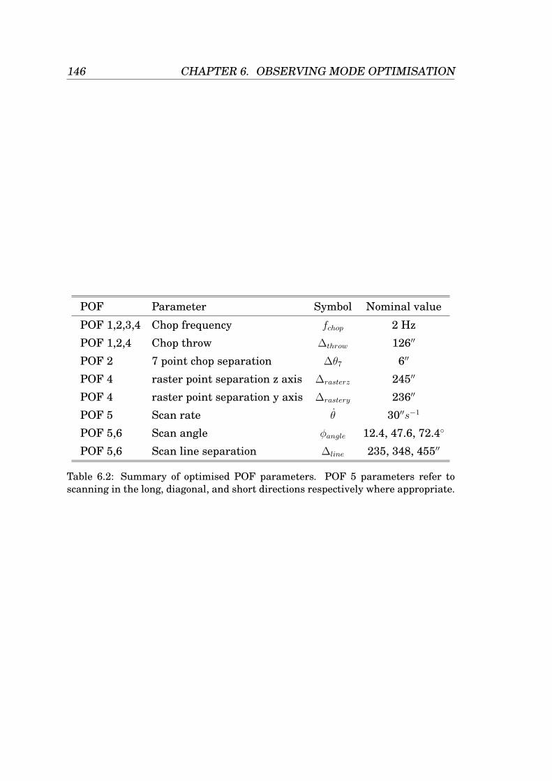
146 CHAPTER 6. OBSERVING MODE OPTIMISATION
POF Parameter Symbol Nominal value
POF 1,2,3,4 Chop frequency fchop 2 Hz
POF 1,2,4 Chop throw ∆throw 126′′
POF 2 7 point chop separation ∆θ7 6′′
POF 4 raster point separation z axis ∆rasterz 245′′
POF 4 raster point separation y axis ∆rastery 236′′
POF 5 Scan rate θ 30′′s−1
POF 5,6 Scan angle φangle 12.4, 47.6, 72.4
POF 5,6 Scan line separation ∆line 235, 348, 455′′
Table 6.2: Summary of optimised POF parameters. POF 5 parameters refer toscanning in the long, diagonal, and short directions respectively where appropriate.
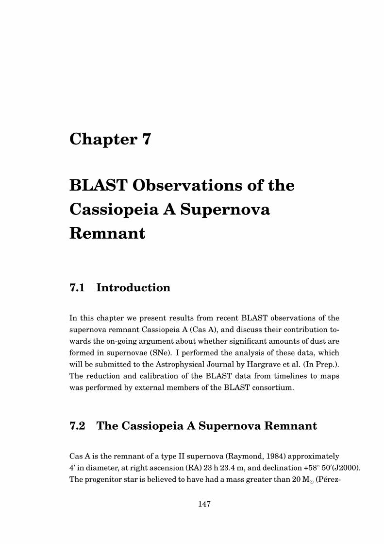
Chapter 7
BLAST Observations of theCassiopeia A SupernovaRemnant
7.1 Introduction
In this chapter we present results from recent BLAST observations of thesupernova remnant Cassiopeia A (Cas A), and discuss their contribution to-wards the on-going argument about whether significant amounts of dust areformed in supernovae (SNe). I performed the analysis of these data, whichwill be submitted to the Astrophysical Journal by Hargrave et al. (In Prep.).The reduction and calibration of the BLAST data from timelines to mapswas performed by external members of the BLAST consortium.
7.2 The Cassiopeia A Supernova Remnant
Cas A is the remnant of a type II supernova (Raymond, 1984) approximately4′ in diameter, at right ascension (RA) 23 h 23.4 m, and declination +58 50′(J2000).The progenitor star is believed to have had a mass greater than 20 M (Perez-
147
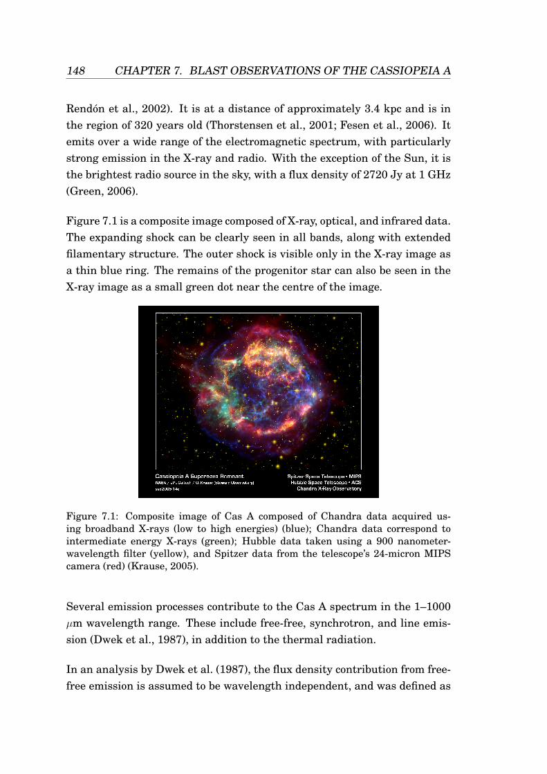
148 CHAPTER 7. BLAST OBSERVATIONS OF THE CASSIOPEIA A
Rendon et al., 2002). It is at a distance of approximately 3.4 kpc and is inthe region of 320 years old (Thorstensen et al., 2001; Fesen et al., 2006). Itemits over a wide range of the electromagnetic spectrum, with particularlystrong emission in the X-ray and radio. With the exception of the Sun, it isthe brightest radio source in the sky, with a flux density of 2720 Jy at 1 GHz(Green, 2006).
Figure 7.1 is a composite image composed of X-ray, optical, and infrared data.The expanding shock can be clearly seen in all bands, along with extendedfilamentary structure. The outer shock is visible only in the X-ray image asa thin blue ring. The remains of the progenitor star can also be seen in theX-ray image as a small green dot near the centre of the image.
Figure 7.1: Composite image of Cas A composed of Chandra data acquired us-ing broadband X-rays (low to high energies) (blue); Chandra data correspond tointermediate energy X-rays (green); Hubble data taken using a 900 nanometer-wavelength filter (yellow), and Spitzer data from the telescope’s 24-micron MIPScamera (red) (Krause, 2005).
Several emission processes contribute to the Cas A spectrum in the 1–1000µm wavelength range. These include free-free, synchrotron, and line emis-sion (Dwek et al., 1987), in addition to the thermal radiation.
In an analysis by Dwek et al. (1987), the flux density contribution from free-free emission is assumed to be wavelength independent, and was defined as
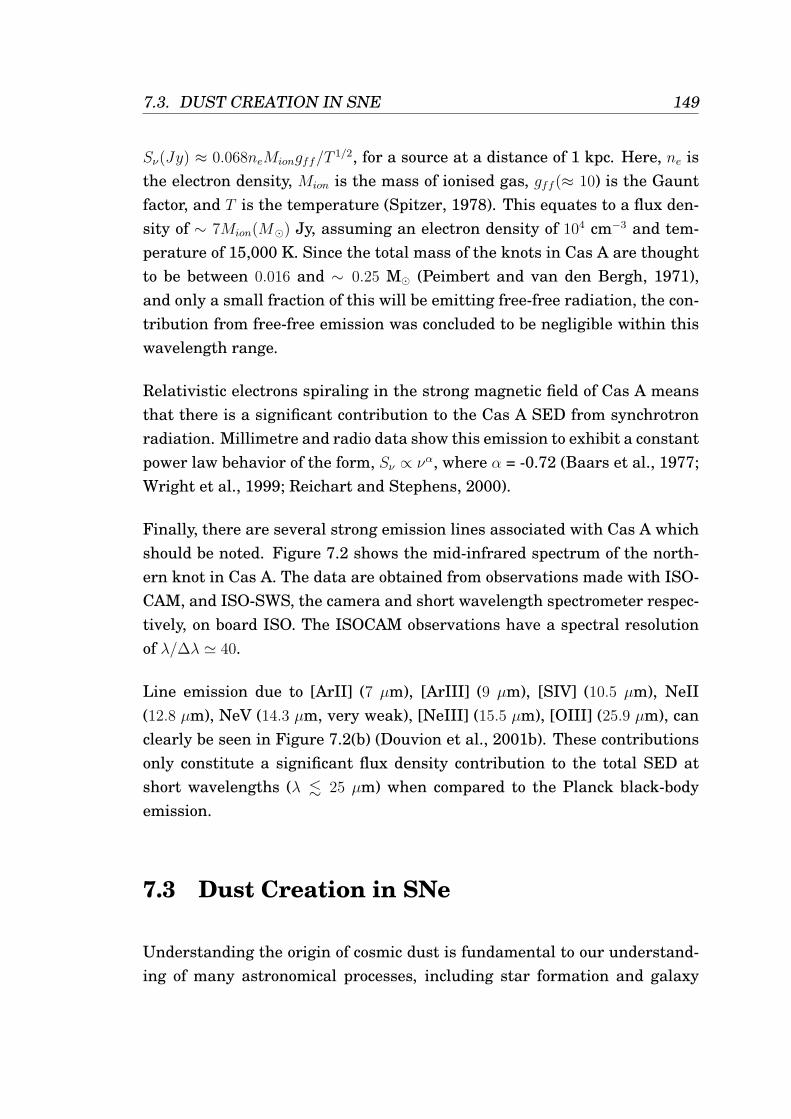
7.3. DUST CREATION IN SNE 149
Sν(Jy) ≈ 0.068neMiongff/T1/2, for a source at a distance of 1 kpc. Here, ne is
the electron density, Mion is the mass of ionised gas, gff (≈ 10) is the Gauntfactor, and T is the temperature (Spitzer, 1978). This equates to a flux den-sity of ∼ 7Mion(M) Jy, assuming an electron density of 104 cm−3 and tem-perature of 15,000 K. Since the total mass of the knots in Cas A are thoughtto be between 0.016 and ∼ 0.25 M (Peimbert and van den Bergh, 1971),and only a small fraction of this will be emitting free-free radiation, the con-tribution from free-free emission was concluded to be negligible within thiswavelength range.
Relativistic electrons spiraling in the strong magnetic field of Cas A meansthat there is a significant contribution to the Cas A SED from synchrotronradiation. Millimetre and radio data show this emission to exhibit a constantpower law behavior of the form, Sν ∝ να, where α = -0.72 (Baars et al., 1977;Wright et al., 1999; Reichart and Stephens, 2000).
Finally, there are several strong emission lines associated with Cas A whichshould be noted. Figure 7.2 shows the mid-infrared spectrum of the north-ern knot in Cas A. The data are obtained from observations made with ISO-CAM, and ISO-SWS, the camera and short wavelength spectrometer respec-tively, on board ISO. The ISOCAM observations have a spectral resolutionof λ/∆λ ' 40.
Line emission due to [ArII] (7 µm), [ArIII] (9 µm), [SIV] (10.5 µm), NeII(12.8 µm), NeV (14.3 µm, very weak), [NeIII] (15.5 µm), [OIII] (25.9 µm), canclearly be seen in Figure 7.2(b) (Douvion et al., 2001b). These contributionsonly constitute a significant flux density contribution to the total SED atshort wavelengths (λ . 25 µm) when compared to the Planck black-bodyemission.
7.3 Dust Creation in SNe
Understanding the origin of cosmic dust is fundamental to our understand-ing of many astronomical processes, including star formation and galaxy
150 CHAPTER 7. BLAST OBSERVATIONS OF THE CASSIOPEIA A
590 T. Douvion et al.: Cassiopeia A dust composition and heating
Fig. 1. Optical image of the northern part ofthe Cas A SNR in the [OIII] lines at 4959and 5007 A, obtained with the SIS instru-ment mounted on the Canada France HawaiiTelescope (CFHT) on August 25th 1998. Thewhite rectangle indicates the size and the posi-tion of the ISO-SWS slit aperture of the obser-vations discussed in this paper
6 8 20 30
10.00
1.00
0.10
0.0110
ISO-SWS
ISOCAM
Fig. 2. Full line: ISOCAM (6–16 µm) and ISO-SWS (16–29µm) fluxes obtained in the aperture plotted in Fig. 1, as afunction of the wavelength. The uncertainties are of ±6 mJy onCAM data and ±1 Jy on SWS data. In addition to the contin-uum emission that is discussed in the paper, we identify forbid-den ionic line emission from [ArII] (7.0µm), [ArIII] (9.0µm),[SIV] (10.5µm), [NeII] (12.8µm), [NeV] (14.3µm, very weak),[NeIII] (15.5µm) and [OIII] (25.9µm). The dashed line is thefit of the continuum emission with Mg-protosilicates heated at169 K, as proposed by ADM99
in ADM99. The slit positions on the sky corresponding tothe two spectra were very close, so that, given the pointinguncertainties of ISO, the main emitting area is probablycontained in both slit apertures.
2.2. ISOCAM observations
The spectrum at wavelengths shorter than 16µm wasobtained with ISOCAM, the camera on board of ISO(Cesarsky et al. 1996). The ISOCAM observations wereperformed on December 5th 1996, with a pixel field of viewof 6′′ and a corresponding total field of view of 3′×3′. Thefield was centered on the northern part of the remnant.For each pixel, we have a spectrum from 6 to 16.5 µm,obtained by rotating the Circular Variable Filter (CVF)
of ISOCAM; the spectral resolution obtained that way isλ/∆λ ' 40. The data reduction was performed with theCam Interactive Analysis2 (CIA) package. We have re-constructed the 7 to 16µm fluxes in the 14′′ by 27′′ SWSaperture, by co-adding the ISOCAM fluxes in this area.The resulting spectrum is shown in Fig. 2. Note that nore-scaling was applied to connect the SWS spectrum andthe ISOCAM spectrum.
3. Dust composition
Following ADM99, we have first tried to fit the spectrumof Fig. 2 with Mg-protosilicates at a temperature of 169 K;the optical constants of Mg-protosilicates have been takenfrom Dorschner et al. (1980). The 16–29µm part of thespectrum is well fitted, but the model predicts a 10µmfeature quite different from the observed one (see Fig. 2).Another material has to be found. The choice of materialsis large, so that we have used, as a starting point, thematerials which are predicted to form in abundance fromSN material, i.e. MgSiO3 (pyroxene) and Al2O3 (Kozasaet al. 1991; Kozasa & Hisato 1997).
We first focused on fitting the feature at 9.5µm.The use of MgSiO3 leads to a better fit of the featurethan Mg-protosilicates; however, the predicted flux is toolow in the 7.5–8.5µm range (see Fig. 3). Whatever thevarious silicates we use, (olivine or pyroxene with variousMg/Fe ratio, Dorschner et al. 1995, various protosilicates,Dorschner et al. 1980, Draine and Lee astronomicalsilicates, Draine & Lee 1984), whatever the dust tem-perature is, the problem persists. The use of Al2O3 isof no help in that region. To solve the problem, we hadto introduce another dust component made of quartz(SiO2). As can be seen in Fig. 3, a good fit of the 9.5µm
2 CIA is a joint development by the ESA astrophysics divi-sion and the ISOCAM consortium.
(a) Optical image of the northern part of the Cas A SN remnant
590 T. Douvion et al.: Cassiopeia A dust composition and heating
Fig. 1. Optical image of the northern part ofthe Cas A SNR in the [OIII] lines at 4959and 5007 A, obtained with the SIS instru-ment mounted on the Canada France HawaiiTelescope (CFHT) on August 25th 1998. Thewhite rectangle indicates the size and the posi-tion of the ISO-SWS slit aperture of the obser-vations discussed in this paper
6 8 20 30
10.00
1.00
0.10
0.0110
ISO-SWS
ISOCAM
Fig. 2. Full line: ISOCAM (6–16 µm) and ISO-SWS (16–29µm) fluxes obtained in the aperture plotted in Fig. 1, as afunction of the wavelength. The uncertainties are of ±6 mJy onCAM data and ±1 Jy on SWS data. In addition to the contin-uum emission that is discussed in the paper, we identify forbid-den ionic line emission from [ArII] (7.0µm), [ArIII] (9.0µm),[SIV] (10.5µm), [NeII] (12.8µm), [NeV] (14.3µm, very weak),[NeIII] (15.5µm) and [OIII] (25.9µm). The dashed line is thefit of the continuum emission with Mg-protosilicates heated at169 K, as proposed by ADM99
in ADM99. The slit positions on the sky corresponding tothe two spectra were very close, so that, given the pointinguncertainties of ISO, the main emitting area is probablycontained in both slit apertures.
2.2. ISOCAM observations
The spectrum at wavelengths shorter than 16µm wasobtained with ISOCAM, the camera on board of ISO(Cesarsky et al. 1996). The ISOCAM observations wereperformed on December 5th 1996, with a pixel field of viewof 6′′ and a corresponding total field of view of 3′×3′. Thefield was centered on the northern part of the remnant.For each pixel, we have a spectrum from 6 to 16.5 µm,obtained by rotating the Circular Variable Filter (CVF)
of ISOCAM; the spectral resolution obtained that way isλ/∆λ ' 40. The data reduction was performed with theCam Interactive Analysis2 (CIA) package. We have re-constructed the 7 to 16µm fluxes in the 14′′ by 27′′ SWSaperture, by co-adding the ISOCAM fluxes in this area.The resulting spectrum is shown in Fig. 2. Note that nore-scaling was applied to connect the SWS spectrum andthe ISOCAM spectrum.
3. Dust composition
Following ADM99, we have first tried to fit the spectrumof Fig. 2 with Mg-protosilicates at a temperature of 169 K;the optical constants of Mg-protosilicates have been takenfrom Dorschner et al. (1980). The 16–29µm part of thespectrum is well fitted, but the model predicts a 10µmfeature quite different from the observed one (see Fig. 2).Another material has to be found. The choice of materialsis large, so that we have used, as a starting point, thematerials which are predicted to form in abundance fromSN material, i.e. MgSiO3 (pyroxene) and Al2O3 (Kozasaet al. 1991; Kozasa & Hisato 1997).
We first focused on fitting the feature at 9.5µm.The use of MgSiO3 leads to a better fit of the featurethan Mg-protosilicates; however, the predicted flux is toolow in the 7.5–8.5µm range (see Fig. 3). Whatever thevarious silicates we use, (olivine or pyroxene with variousMg/Fe ratio, Dorschner et al. 1995, various protosilicates,Dorschner et al. 1980, Draine and Lee astronomicalsilicates, Draine & Lee 1984), whatever the dust tem-perature is, the problem persists. The use of Al2O3 isof no help in that region. To solve the problem, we hadto introduce another dust component made of quartz(SiO2). As can be seen in Fig. 3, a good fit of the 9.5µm
2 CIA is a joint development by the ESA astrophysics divi-sion and the ISOCAM consortium.
(b) Mid-infrared spectrum of the Cas A SN remnant
Figure 7.2: (a) Optical image of the northern part of the Cas A SN remnant in the[OIII] lines at 4959 and 5007 A; (b) Mid-infrared spectrum of the region outlined inpart (a), taken with ISOCAM (6–16µm) and ISO- SWS (16–29µm) (Douvion et al.,2001b).
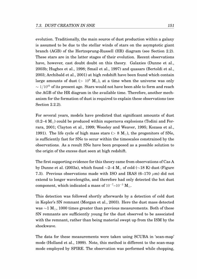
7.3. DUST CREATION IN SNE 151
evolution. Traditionally, the main source of dust production within a galaxyis assumed to be due to the stellar winds of stars on the asymptotic giantbranch (AGB) of the Hertzsprung-Russell (HR) diagram (see Section 2.2).These stars are in the latter stages of their evolution. Recent observationshave, however, cast doubt doubt on this theory. Galaxies (Dunne et al.,2003b; Hughes et al., 1998; Smail et al., 1997) and quasars (Bertoldi et al.,2003; Archibald et al., 2001) at high redshift have been found which containlarge amounts of dust (> 108 M), at a time when the universe was only∼ 1/10th of its present age. Stars would not have been able to form and reachthe AGB of the HR diagram in the available time. Therefore, another mech-anism for the formation of dust is required to explain these observations (seeSection 2.2.2).
For several years, models have predicted that significant amounts of dust(0.2–4 M) could be produced within supernova explosions (Todini and Fer-rara, 2001; Clayton et al., 1999; Woosley and Weaver, 1995; Kozasa et al.,1991). The life cycle of high mass stars (> 8 M), the progenitors of SNe,is sufficiently fast for SNe to occur within the timescales constrained by theobservations. As a result SNe have been proposed as a possible solution tothe origin of the excess dust seen at high redshift.
The first supporting evidence for this theory came from observations of Cas Aby Dunne et al. (2003a), which found ∼2–4 M of cold (∼18 K) dust (Figure7.3). Previous observations made with ISO and IRAS (6–170 µm) did notextend to longer wavelengths, and therefore had only detected the hot dustcomponent, which indicated a mass of 10−7–10−3 M.
This detection was followed shortly afterwards by a detection of cold dustin Kepler’s SN remnant (Morgan et al., 2003). Here the dust mass detectedwas ∼1 M, 1000 times greater than previous measurements. Both of theseSN remnants are sufficiently young for the dust observed to be associatedwith the remnant, rather than being material swept up from the ISM by theshockwave.
The data for these measurements were taken using SCUBA in ‘scan-map’mode (Holland et al., 1999). Note, this method is different to the scan-mapmode employed by SPIRE. The observation was performed while chopping,
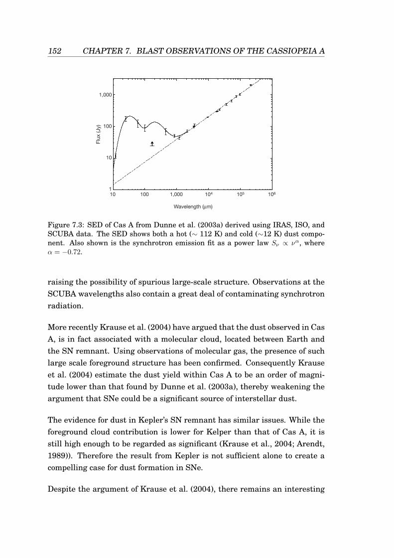
152 CHAPTER 7. BLAST OBSERVATIONS OF THE CASSIOPEIA A
..............................................................
Type II supernovae as a significantsource of interstellar dustLoretta Dunne*, Stephen Eales*, Rob Ivison†, Haley Morgan*& Mike Edmunds*
* Department of Physics and Astronomy, Cardiff University, 5 The Parade,Cardiff CF24 3YB, UK† Astronomy Technology Centre, Royal Observatory, Blackford Hill, EdinburghEH9 3HJ, UK.............................................................................................................................................................................
Large amounts of dust (>108M () have recently been discoveredin high-redshift quasars1,2 and galaxies3–5 corresponding to a timewhen the Universe was less than one-tenth of its present age. Thestellar winds produced by stars in the late stages of theirevolution (on the asymptotic giant branch of the Hertzsprung–Russell diagram) are thought to be the main source of dust ingalaxies, but they cannot produce that dust on a short enoughtimescale6 (<1 Gyr) to explain the results in the high-redshiftgalaxies. Supernova explosions of massive stars (type II) are alsoa potential source, with models predicting 0.2–4M( of dust7–10.As massive stars evolve rapidly, on timescales of a few Myr, these
supernovae could be responsible for the high-redshiftdust. Observations11–13 of supernova remnants in the MilkyWay, however, have hitherto revealed only 1027–1023M( each,which is insufficient to explain the high-redshift data. Here wereport the detection of ,2–4M( of cold dust in the youngestknown Galactic supernova remnant, Cassiopeia A. This obser-vation implies that supernovae are at least as important as stellarwinds in producing dust in our Galaxy and would have been thedominant source of dust at high redshifts.
Over the past three decades, many searches for dust in supernovaremnants have been made in the mid and far-infrared (6–100 mm).Remnants must be studied when they are young, before they haveswept up large masses of interstellar material which makes itdifficult to distinguish dust formed in the ejecta from that presentin the interstellar medium (ISM) prior to the explosion. Thehandful of Galactic remnants which are both young and closeenough (Cas A, Kepler and Tycho) have been studied with theInfrared Astronomical Satellite (IRAS) and the Infrared SpaceObservatory (ISO), but although dust at 100–200 K has beendetected, the dust mass deduced is only 1027–1023M(, manyorders of magnitude lower than the solar mass quantities pre-dicted11–13. The formation of dust in the recent supernova 1987Ahas been implied indirectly from the fading of the silicate line andincrease in 10 mm emission14, although the quantity is heavilydependent on the assumptions made about the clumpiness of thedust (if the dust is uniform, the observations imply a very low
Figure 1 SCUBA 850-mm image of Cas A at a resolution of 15 arcsec. The data were
taken in scan map mode and reduced in a standard way using SURF. Scan map is
known to produce artefacts on large angular scales on the final image and these
remain the limitation on the accuracy of the absolute flux measurement and
morphology. On the 850-mm image, the linear baseline removal left an area of diffuse
emission to the west of the remnant which we believe was an artefact. After
subtraction of a surface which removed this feature the loss of flux in the remnant was
5 Jy. We confirmed the accuracy of the absolute flux level of the maps by making new
photometric measurements with SCUBA at several positions on the remnant in
December 2002. The quoted 1j uncertainty on the fluxes is a combination of
calibration errors (5–10% and 15–20% at 850 and 450 mm), plus the range of fluxes
from the maps which agreed with the photometry. The integrated fluxes were corrected
for the error lobe contribution (derived from maps of Uranus) by dividing by 1.2 at
850 mm and 2.0 at 450 mm.
Figure 2 The SED of Cas A from the mid-infrared to the radio. All fluxes are integrated.
The radio spectrum is fitted with a power-law slope with spectral index a ¼ 20.72. The
radio data19,23–28 have been scaled to the epoch of our Cas A observation (1998.4) using a
recent study23 which found that the flux decrease of Cas A was independent of frequency
at about 0.6–0.7% yr21. The IRAS points are the averages of the literature values13,29
with the error bars indicating the range of fluxes. SCUBA fluxes are 50.8 ^ 5.6 Jy at
850 mm and 69.8 ^ 16.1 Jy at 450 mm. The synchrotron contribution is 34.9 Jy at 850 mm
and 22.1 Jy at 450 mm. The fit to the far-infrared/submm points is for a two-temperature
grey body with b ¼ 0.9, Tw ¼ 112 K, Tc ¼ 18 K and for 700 times more mass in the cold
component than in the hot. We have fitted five parameters to six data points and therefore
the fit is just constrained. The uncertainties in the SED parameters are given in Table 1.
Clearly, the submm points at 450 and 850 mm lie above the extrapolation of the radio
synchrotron spectrum. The point at 1.2 mm (ref. 28) is not of sufficient accuracy to
determine an excess, but is consistent with our higher frequency measurements. Longer
wavelength ISO measurements30 of Cas A at 170 mm suggested that dust at ,30 K
may have been present (implying of order 0.15M ( of dust), however, the poor angular
resolution of ISO at these wavelengths made a separation of the remnant and background
emission impossible. The ISO flux is therefore a lower limit (R.J. Tuffs, personal
communication).
letters to nature
NATURE | VOL 424 | 17 JULY 2003 | www.nature.com/nature 285© 2003 Nature Publishing Group
Figure 7.3: SED of Cas A from Dunne et al. (2003a) derived using IRAS, ISO, andSCUBA data. The SED shows both a hot (∼ 112 K) and cold (∼12 K) dust compo-nent. Also shown is the synchrotron emission fit as a power law Sν ∝ να, whereα = −0.72.
raising the possibility of spurious large-scale structure. Observations at theSCUBA wavelengths also contain a great deal of contaminating synchrotronradiation.
More recently Krause et al. (2004) have argued that the dust observed in CasA, is in fact associated with a molecular cloud, located between Earth andthe SN remnant. Using observations of molecular gas, the presence of suchlarge scale foreground structure has been confirmed. Consequently Krauseet al. (2004) estimate the dust yield within Cas A to be an order of magni-tude lower than that found by Dunne et al. (2003a), thereby weakening theargument that SNe could be a significant source of interstellar dust.
The evidence for dust in Kepler’s SN remnant has similar issues. While theforeground cloud contribution is lower for Kelper than that of Cas A, it isstill high enough to be regarded as significant (Krause et al., 2004; Arendt,1989)). Therefore the result from Kepler is not sufficient alone to create acompelling case for dust formation in SNe.
Despite the argument of Krause et al. (2004), there remains an interesting
7.4. OBSERVATIONS OF CAS A WITH BLAST 153
relation between the structure of the Cas A SN remnant, and the emissionfrom the foreground cloud, which suggests that there could still be cold dustassociated with the remnant.
7.4 Observations of Cas A with BLAST
Neither the SCUBA nor Spitzer observations sample the cold dust compo-nent seen towards Cas A particularly well. The SCUBA 450 µm and 850 µmobservations provide measurements longward of the peak cold dust emission(Figure 7.3), while Spitzer data are only available at shorter wavelengths(3.6 – 160 µm). In addition, the Spitzer 160 µm band data are poorly sam-pled, with large holes in the map. The BLAST bands span this missing wave-length range well, providing three valuable additional measurements withinthe cold dust region of the SED. BLAST is also, like Spitzer (and SPIRE inscan-map mode), a direct measurement system, and therefore does not needto chop. As a result, these data will not be susceptible to the spurious largescale structure issues that plague the SCUBA observations. The high map-ping speed of BLAST means that in addition to Cas A, it is possible to map alarge area (30′) surrounding the SN remnant, giving data for the foregroundcloud structure.
Here I describe the BLAST observations performed, and the analysis of thesedata. I derive an SED for both the cloud, and SN remnant sources within themaps, and discuss the implications of these results in terms of the possiblecold dust associated with Cas A.
7.4.1 The Data
BLAST performed a ‘cap’ observation of Cas A during the first LDB flightin July 2005. In this observing mode the telescope slews backwards andforwards in azimuth while slowly, and at a constant rate, increasing in alti-tude. The slew is varied such that a circular region of sky is observed (seeFigure 7.4). At the start of the scan the azimuth scan is below the minimum
154 CHAPTER 7. BLAST OBSERVATIONS OF THE CASSIOPEIA A
angular scale, resulting in the flattened regions seen at the top and bottom(beginning and end) of the scan pattern shown.
A slew rate of 6′s−1 and altitude scan rate of 3.25′ per scan line (1/2 an array)were used to perform the observation. Due to flight time limitation, it wasonly possible to perform 1.25 scan maps. The maps were ∼40′ × 60′ in size.
Figure 7.4: Schematic diagram of a typical BLAST ‘cap’ scanning pattern.
Early in the flight it was found that the telescope was not correctly focused.Modelling of the distortion suggests that this could have been due to the sec-ondary mirror being several centimetres from its designed location. Whenthe telescope was recovered, part of the secondary support structure wasdamaged. This could have happened in launch or during landing. If thisfault developed during the launch, then this could explain the focusing er-ror. The result of this was a distortion of the telescope beam in the threewavelength bands, as shown in Figure 7.5.
The beam deformation resulted in a severely degraded angular resolution inall bands. Using Figure 7.5 it can be seen that the beam sizes for all threebands are ∼3-4′, rather than the nominal values of 30, 41, and 59′′ for thePSW, PMW, and PLW bands respectively. Consequently it was not possibleto resolve structure within the 4′ diameter SN remnant. I were thereforeunable to determine if there was significant cloud structure on scales smaller
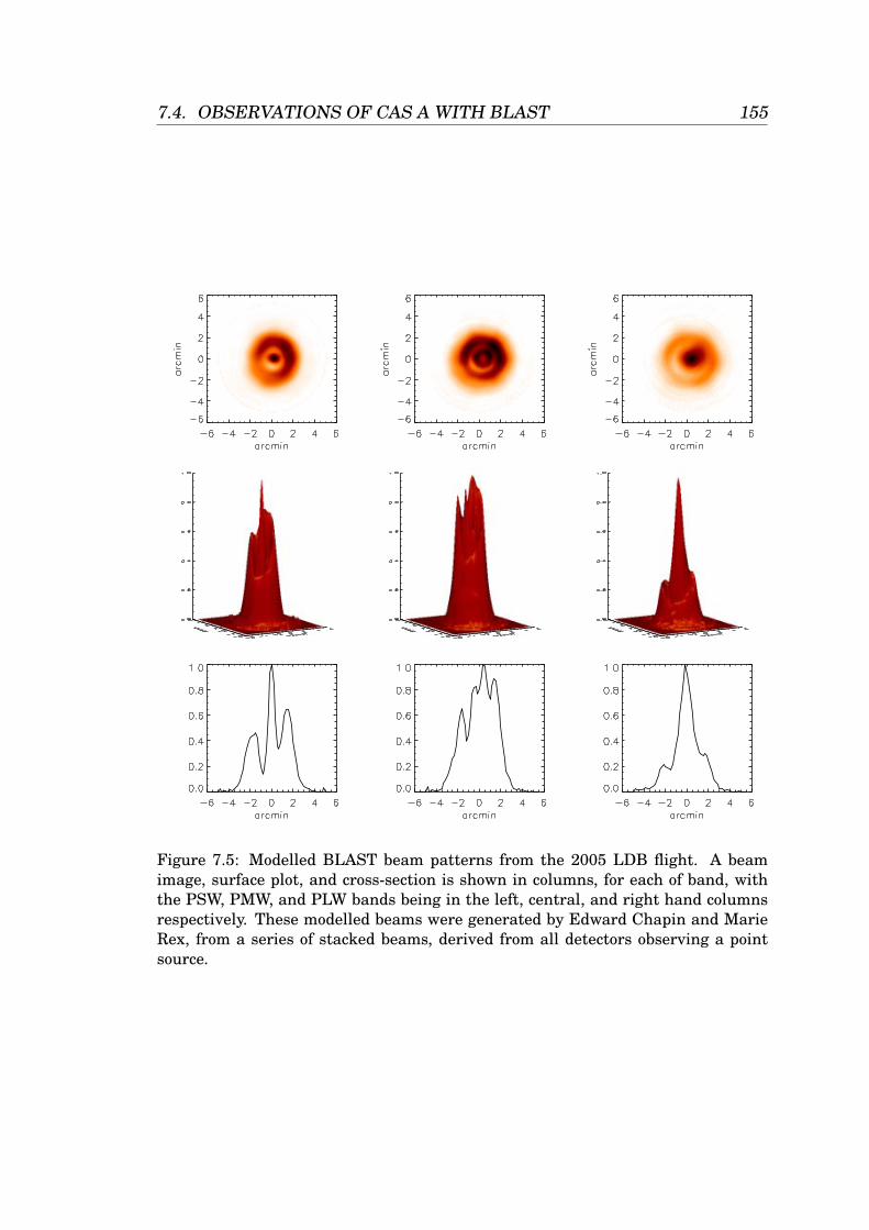
7.4. OBSERVATIONS OF CAS A WITH BLAST 155
Figure 7.5: Modelled BLAST beam patterns from the 2005 LDB flight. A beamimage, surface plot, and cross-section is shown in columns, for each of band, withthe PSW, PMW, and PLW bands being in the left, central, and right hand columnsrespectively. These modelled beams were generated by Edward Chapin and MarieRex, from a series of stacked beams, derived from all detectors observing a pointsource.
156 CHAPTER 7. BLAST OBSERVATIONS OF THE CASSIOPEIA A
than that of the SN remnant.
The BLAST data are still useful however, despite the focusing problem. Withthese data I am able to measure the flux density of both the SN remnantand the surrounding cloud in all three bands, and hence further constrainwhatever cold dust component might be present. The direct measurement(i.e. no chopping) will also provide a information on the surrounding cloudstructure.
7.5 Data Reduction
The BLAST TOD was reduced to map form by Guillaume Patanchon at theUniversity of British Columbia (UBC). This work was performed with con-tributions from the entire BLAST team. Maximum likelihood maps weregenerated using a custom routine, however, due to the low level of redun-dancy and lack of cross-linking in the Cas A observations, the output showedlittle improvement in comparison to a naıve map. As a result, the data werehigh pass filtered before the map was made to reduce the low frequencynoise. Prior to making the map, the data were also de-spiked, flat-fielded,and calibrated, and the detector response function deconvolved. The cali-bration constant for each waveband was derived from an SED of CRL 2688,constructed from UKT14 (Duncan et al., 1990), SCUBA, SHARC II (Dowellet al., 2003), and ISO data. A pointing solution was also applied.
7.6 Data Analysis and Results
The aim of our analysis was to derive two SEDs, one in the direction ofthe foreground cloud (SEDcloud), and the other in the direction of Cas A(SEDCasA). This second SED would contain contributions from both the SNremnant and the cloud combined. We would then be able to compare theSED of the cloud, with the cold component seen in the SED of Cas A. A sim-ilar SED for both the cloud and cold SN remnant component would suggest
7.6. DATA ANALYSIS AND RESULTS 157
that the measured dust was most likely associated with the cloud, and notthe SN remant.
7.6.1 Maps
In addition to BLAST data, I also obtained data from the MSX (Mill, 1994)and IRAS (Neugebauer et al., 1984) archives (Figures 7.6 and 7.7). Thisallows me to determine SEDs which span a wavelength range of 8–520 µm,thus incorporating the hot and cold peaks seen in Figure 7.3. These data areshown in Figures 7.6 and 7.7 in the form of maps, along with the SCUBA850 µm map from Dunne et al. (2003a) for comparison. All of the maps inthis figure contain the same 50′ × 50′ region of sky centred on Cas A.
Both the IRAS and BLAST maps are confusion noise limited, while the MSXmaps are instrument noise limited. The SN remnant can be clearly seenin Figures 7.6(a-f), with significant SN remnant structure being visible inthe first MSX band. Conversely, there is very little structure seen on scaleslarger than the size of the SN remnant at these wavelengths, with suchstructure only really becoming visible at wavelengths longward of 60 µm. Acommon large scale cloud structure can be seen in these longer wavelengthbands (Figures 7.7(g-k)), peaking between the IRAS 100 µm, and BLAST 250µm bands. A distinctive knot of material can clearly be seen to the upper leftof the SN remnant in each of these images. The position of Cas A and theknot of cloud material are shown on the IRAS 100 µm map by an X and a ∆
respectively.
Due to the focusing problem mentioned above, the BLAST maps have in-sufficient resolution to identify any sub-remnant scale structure in the fore-ground cloud. It is therefore difficult to assess the influence such structuremight have had on the reliability of the SCUBA measurements. However, us-ing the limited extent of the SCUBA map as a guide to the chop throw, andthe BLAST 520 µm map as representative of the surrounding cloud struc-ture, it is possible to assess the credibility of the chopped observing func-tion used by SCUBA, given the large scale cloud structure. The large varia-tion seen in cloud structure immediately adjacent to the edge of the SCUBA
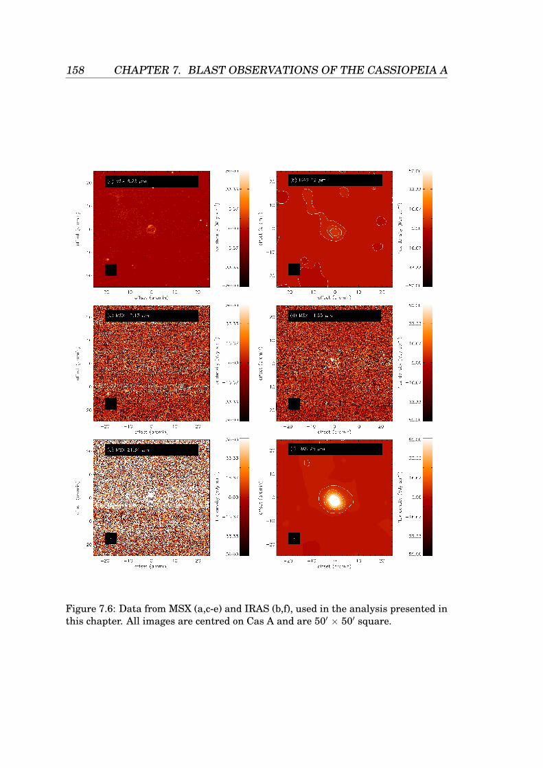
158 CHAPTER 7. BLAST OBSERVATIONS OF THE CASSIOPEIA A
Figure 7.6: Data from MSX (a,c-e) and IRAS (b,f), used in the analysis presented inthis chapter. All images are centred on Cas A and are 50′ × 50′ square.
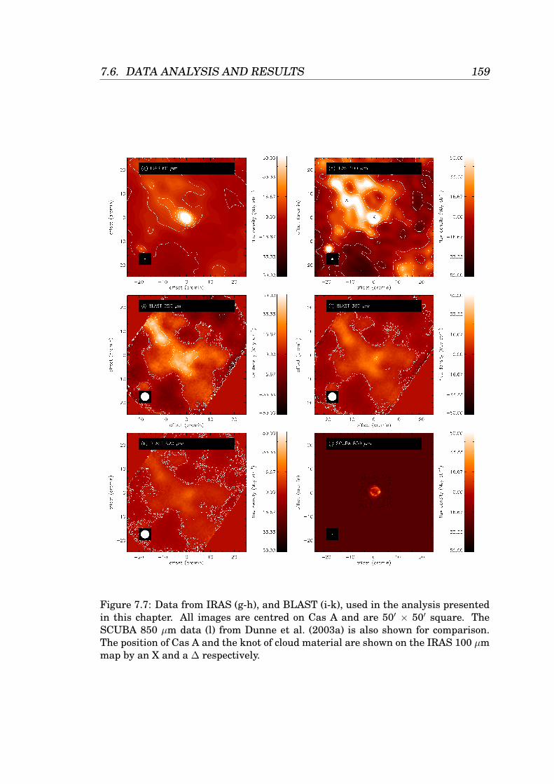
7.6. DATA ANALYSIS AND RESULTS 159
Figure 7.7: Data from IRAS (g-h), and BLAST (i-k), used in the analysis presentedin this chapter. All images are centred on Cas A and are 50′ × 50′ square. TheSCUBA 850 µm data (l) from Dunne et al. (2003a) is also shown for comparison.The position of Cas A and the knot of cloud material are shown on the IRAS 100 µmmap by an X and a ∆ respectively.
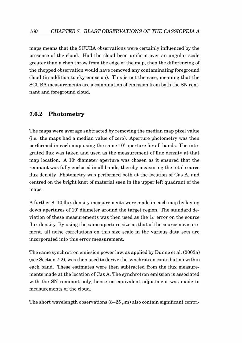
160 CHAPTER 7. BLAST OBSERVATIONS OF THE CASSIOPEIA A
maps means that the SCUBA observations were certainly influenced by thepresence of the cloud. Had the cloud been uniform over an angular scalegreater than a chop throw from the edge of the map, then the differencing ofthe chopped observation would have removed any contaminating foregroundcloud (in addition to sky emission). This is not the case, meaning that theSCUBA measurements are a combination of emission from both the SN rem-nant and foreground cloud.
7.6.2 Photometry
The maps were average subtracted by removing the median map pixel value(i.e. the maps had a median value of zero). Aperture photometry was thenperformed in each map using the same 10′ aperture for all bands. The inte-grated flux was taken and used as the measurement of flux density at thatmap location. A 10′ diameter aperture was chosen as it ensured that theremnant was fully enclosed in all bands, thereby measuring the total sourceflux density. Photometry was performed both at the location of Cas A, andcentred on the bright knot of material seen in the upper left quadrant of themaps.
A further 8–10 flux density measurements were made in each map by layingdown apertures of 10′ diameter around the target region. The standard de-viation of these measurements was then used as the 1σ error on the sourceflux density. By using the same aperture size as that of the source measure-ment, all noise correlations on this size scale in the various data sets areincorporated into this error measurement.
The same synchrotron emission power law, as applied by Dunne et al. (2003a)(see Section 7.2), was then used to derive the synchrotron contribution withineach band. These estimates were then subtracted from the flux measure-ments made at the location of Cas A. The synchrotron emission is associatedwith the SN remnant only, hence no equivalent adjustment was made tomeasurements of the cloud.
The short wavelength observations (8–25 µm) also contain significant contri-
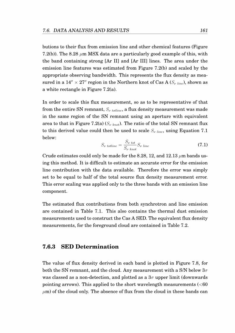
7.6. DATA ANALYSIS AND RESULTS 161
butions to their flux from emission line and other chemical features (Figure7.2(b)). The 8.28 µm MSX data are a particularly good example of this, withthe band containing strong [Ar II] and [Ar III] lines. The area under theemission line features was estimated from Figure 7.2(b) and scaled by theappropriate observing bandwidth. This represents the flux density as mea-sured in a 14′′ × 27′′ region in the Northern knot of Cas A (Sν line), shown asa white rectangle in Figure 7.2(a).
In order to scale this flux measurement, so as to be representative of thatfrom the entire SN remnant, Sν totline, a flux density measurement was madein the same region of the SN remnant using an aperture with equivalentarea to that in Figure 7.2(a) (Sν knot). The ratio of the total SN remnant fluxto this derived value could then be used to scale Sν line, using Equation 7.1below:
Sν totline =Sν totSν knot
Sν line (7.1)
Crude estimates could only be made for the 8.28, 12, and 12.13 µm bands us-ing this method. It is difficult to estimate an accurate error for the emissionline contribution with the data available. Therefore the error was simplyset to be equal to half of the total source flux density measurement error.This error scaling was applied only to the three bands with an emission linecomponent.
The estimated flux contributions from both synchrotron and line emissionare contained in Table 7.1. This also contains the thermal dust emissionmeasurements used to construct the Cas A SED. The equivalent flux densitymeasurements, for the foreground cloud are contained in Table 7.2.
7.6.3 SED Determination
The value of flux density derived in each band is plotted in Figure 7.8, forboth the SN remnant, and the cloud. Any measurement with a S/N below 3σwas classed as a non-detection, and plotted as a 3σ upper limit (downwardspointing arrows). This applied to the short wavelength measurements (<60µm) of the cloud only. The absence of flux from the cloud in these bands can
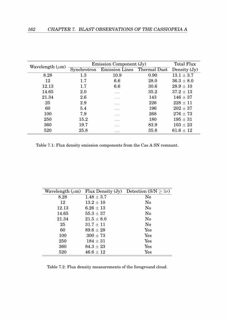
162 CHAPTER 7. BLAST OBSERVATIONS OF THE CASSIOPEIA A
Wavelength (µm) Emission Component (Jy) Total FluxSynchrotron Emission Lines Thermal Dust Density (Jy)
8.28 1.3 10.9 0.90 13.1 ± 3.712 1.7 6.6 28.0 36.3 ± 8.0
12.13 1.7 6.6 30.6 28.9 ± 1014.65 2.0 . . . 35.2 37.2 ± 1321.34 2.6 . . . 143 146 ± 37
25 2.9 . . . 226 228 ± 1160 5.4 . . . 196 202 ± 37100 7.9 . . . 268 276 ± 73250 15.2 . . . 180 195 ± 31360 19.7 . . . 83.9 103 ± 23520 25.8 . . . 35.8 61.6 ± 12
Table 7.1: Flux density emission components from the Cas A SN remnant.
Wavelength (µm) Flux Density (Jy) Detection (S/N ≥ 3σ)8.28 1.48 ± 3.7 No12 13.2 ± 10 No
12.13 6.26 ± 13 No14.65 55.3 ± 37 No21.34 21.5 ± 8.0 No
25 31.7 ± 11 No60 89.6 ± 28 Yes100 300 ± 73 Yes250 184 ± 31 Yes360 84.3 ± 23 Yes520 46.6 ± 12 Yes
Table 7.2: Flux density measurements of the foreground cloud.
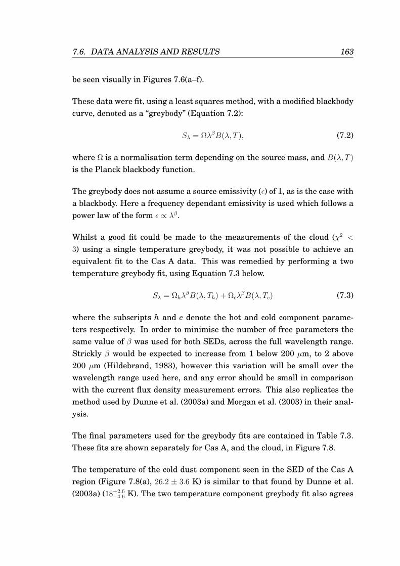
7.6. DATA ANALYSIS AND RESULTS 163
be seen visually in Figures 7.6(a–f).
These data were fit, using a least squares method, with a modified blackbodycurve, denoted as a “greybody” (Equation 7.2):
Sλ = ΩλβB(λ, T ), (7.2)
where Ω is a normalisation term depending on the source mass, and B(λ, T )
is the Planck blackbody function.
The greybody does not assume a source emissivity (ε) of 1, as is the case witha blackbody. Here a frequency dependant emissivity is used which follows apower law of the form ε ∝ λβ.
Whilst a good fit could be made to the measurements of the cloud (χ2 <
3) using a single temperature greybody, it was not possible to achieve anequivalent fit to the Cas A data. This was remedied by performing a twotemperature greybody fit, using Equation 7.3 below.
Sλ = ΩhλβB(λ, Th) + Ωcλ
βB(λ, Tc) (7.3)
where the subscripts h and c denote the hot and cold component parame-ters respectively. In order to minimise the number of free parameters thesame value of β was used for both SEDs, across the full wavelength range.Strickly β would be expected to increase from 1 below 200 µm, to 2 above200 µm (Hildebrand, 1983), however this variation will be small over thewavelength range used here, and any error should be small in comparisonwith the current flux density measurement errors. This also replicates themethod used by Dunne et al. (2003a) and Morgan et al. (2003) in their anal-ysis.
The final parameters used for the greybody fits are contained in Table 7.3.These fits are shown separately for Cas A, and the cloud, in Figure 7.8.
The temperature of the cold dust component seen in the SED of the Cas Aregion (Figure 7.8(a), 26.2 ± 3.6 K) is similar to that found by Dunne et al.(2003a) (18+2.6
−4.6 K). The two temperature component greybody fit also agrees
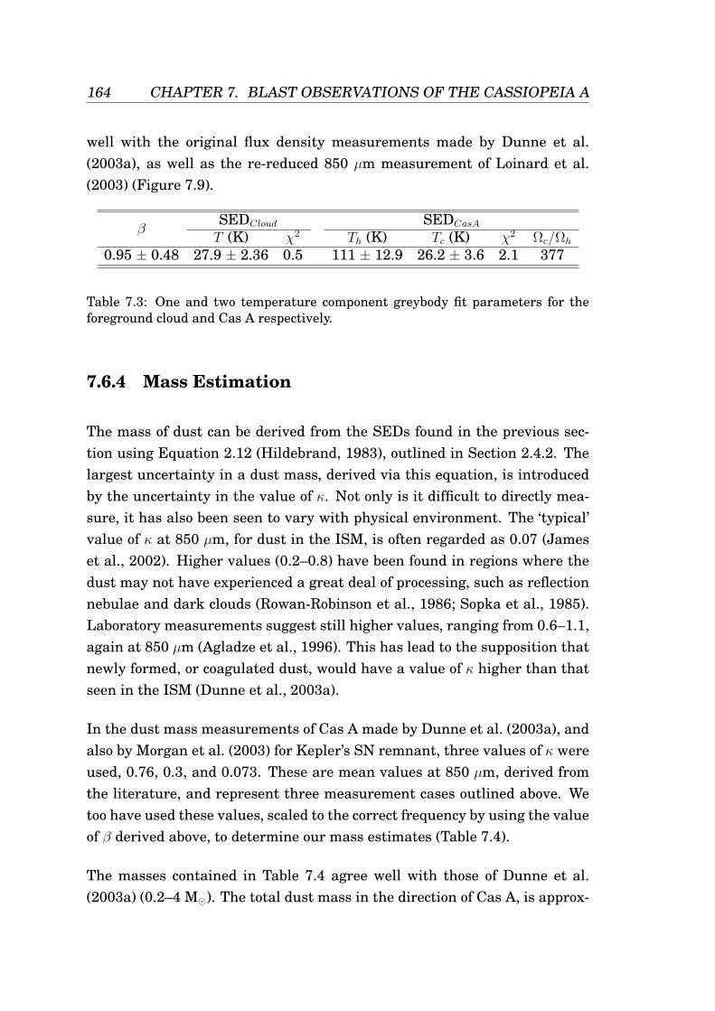
164 CHAPTER 7. BLAST OBSERVATIONS OF THE CASSIOPEIA A
well with the original flux density measurements made by Dunne et al.(2003a), as well as the re-reduced 850 µm measurement of Loinard et al.(2003) (Figure 7.9).
βSEDCloud SEDCasA
T (K) χ2 Th (K) Tc (K) χ2 Ωc/Ωh
0.95 ± 0.48 27.9 ± 2.36 0.5 111 ± 12.9 26.2 ± 3.6 2.1 377
Table 7.3: One and two temperature component greybody fit parameters for theforeground cloud and Cas A respectively.
7.6.4 Mass Estimation
The mass of dust can be derived from the SEDs found in the previous sec-tion using Equation 2.12 (Hildebrand, 1983), outlined in Section 2.4.2. Thelargest uncertainty in a dust mass, derived via this equation, is introducedby the uncertainty in the value of κ. Not only is it difficult to directly mea-sure, it has also been seen to vary with physical environment. The ‘typical’value of κ at 850 µm, for dust in the ISM, is often regarded as 0.07 (Jameset al., 2002). Higher values (0.2–0.8) have been found in regions where thedust may not have experienced a great deal of processing, such as reflectionnebulae and dark clouds (Rowan-Robinson et al., 1986; Sopka et al., 1985).Laboratory measurements suggest still higher values, ranging from 0.6–1.1,again at 850 µm (Agladze et al., 1996). This has lead to the supposition thatnewly formed, or coagulated dust, would have a value of κ higher than thatseen in the ISM (Dunne et al., 2003a).
In the dust mass measurements of Cas A made by Dunne et al. (2003a), andalso by Morgan et al. (2003) for Kepler’s SN remnant, three values of κ wereused, 0.76, 0.3, and 0.073. These are mean values at 850 µm, derived fromthe literature, and represent three measurement cases outlined above. Wetoo have used these values, scaled to the correct frequency by using the valueof β derived above, to determine our mass estimates (Table 7.4).
The masses contained in Table 7.4 agree well with those of Dunne et al.(2003a) (0.2–4 M). The total dust mass in the direction of Cas A, is approx-
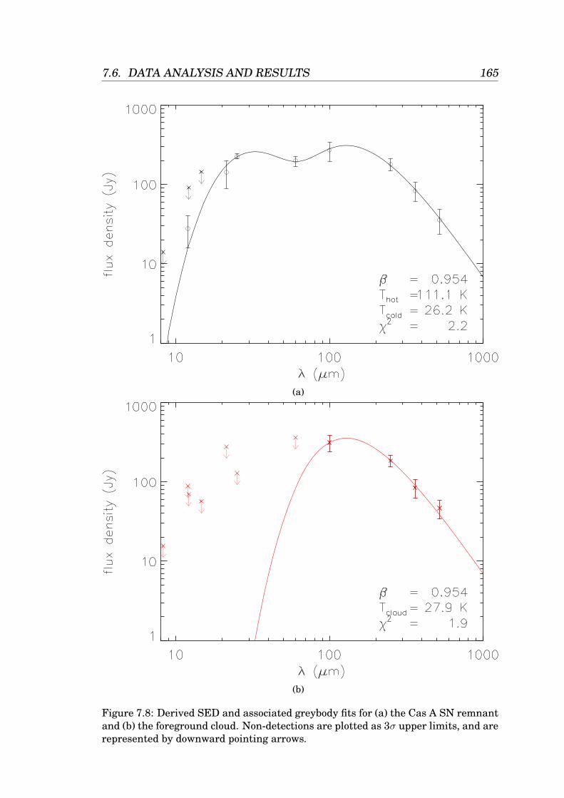
7.6. DATA ANALYSIS AND RESULTS 165
(a)
(b)
Figure 7.8: Derived SED and associated greybody fits for (a) the Cas A SN remnantand (b) the foreground cloud. Non-detections are plotted as 3σ upper limits, and arerepresented by downward pointing arrows.
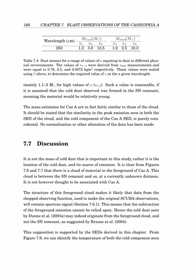
166 CHAPTER 7. BLAST OBSERVATIONS OF THE CASSIOPEIA A
Wavelength (µm) MCasA(M) Mcloud(M)κ1 κ2 κ3 κ1 κ2 κ3
250 1.2 3.0 12.5 1.0 2.5 10.3
Table 7.4: Dust masses for a range of values of κ equating to dust in different phys-ical environments. The values of κ1−3 were derived from κ850 measurements andwere equal to 0.76, 0.3, and 0.0072 kgm2 respectively. These values were scaledusing β above, to determine the required value of κ at the a given wavelength.
imately 1.1–3 M for high values of κ (κ1,2). Such a value is reasonable, ifit is assumed that the cold dust observed was formed in the SN remnant,meaning the material would be relatively young.
The mass estimates for Cas A are in fact fairly similar to those of the cloud.It should be stated that the similarity in the peak emission seen in both theSED of the cloud, and the cold component of the Cas A SED, is purely coin-cidental. No normalisation or other alteration of the data has been made.
7.7 Discussion
It is not the mass of cold dust that is important in this study, rather it is thelocation of the cold dust, and its source of emission. It is clear from Figures7.6 and 7.7 that there is a cloud of material in the foreground of Cas A. Thiscloud is between the SN remnant and us, at a currently unknown distance.It is not however thought to be associated with Cas A.
The structure of this foreground cloud makes it likely that data from thechopped observing function, used to make the original SCUBA observations,will contain spurious signal (Section 7.6.1). This means that the subtractionof the foreground emission cannot be relied upon. Hence the cold dust seenby Dunne et al. (2003a) may indeed originate from the foreground cloud, andnot the SN remnant, as suggested by Krause et al. (2004).
This supposition is supported by the SEDs derived in this chapter. FromFigure 7.9, we can identify the temperature of both the cold component seen
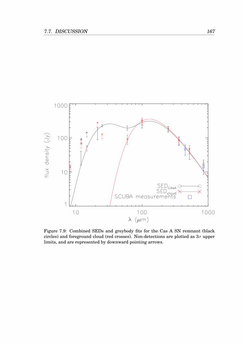
7.7. DISCUSSION 167
Figure 7.9: Combined SEDs and greybody fits for the Cas A SN remnant (blackcircles) and foreground cloud (red crosses). Non-detections are plotted as 3σ upperlimits, and are represented by downward pointing arrows.
168 CHAPTER 7. BLAST OBSERVATIONS OF THE CASSIOPEIA A
towards Cas A, 27.9±2.4 K, and that of the cloud, well away from the rem-nant, 26.2±3.6 K. The agreement of these two values strongly suggests thatthe detection of significant quantities of cold dust in Cas A was due to con-tamination by emission from the foreground cloud.
The peak of the derived Cas A SED is also greater than that seen by Dunneet al. (2003a) (Figure 7.3). This is a consequence of using a larger aperturethan Dunne et al. (2003a), when performing the photometry. The largeraperture results in more flux from the cloud being included in the measure-ment. If the cold dust were associated only with the SN remnant, thenthere should be no increase in flux for aperture sizes greater than that ofthe shock-front (diameter ∼4′).
This result does not exclude the possibility of cold dust being present in CasA; it merely means that if it is present, it must be at a temperature nearto that of the foreground cloud. This makes a conclusive detection of dustextremely difficult. However, if cold dust were present in any great quantity,it would be reasonable to expect the emission to be significantly greater inthe region of Cas A, than that of the surrounding cloud. The measurementsabove show Cas A to be only ∼ 6% brighter than the nearby knot of materialused to derive the cloud SED in the 250 µm band. In fact, Cas A registersas a ∼ 2.5σ detection in this band when measured against the overall cloudconfusion noise in the map, rather than the local confusion, used to derivethe earlier noise measurement.
The presence of a large knot of material, directly at the location of Cas A,would be required to explain these observations, assuming that there is nocold dust in Cas A. It would seem to be extremely improbable that this knotof material should contain the peak emission in the map, exactly at the po-sition of Cas A, and have no contribution from the SN remnant.
Further observations are needed of more SN remnants in order to resolvethis issue. Observations with higher angular resolution, such as those achiev-able with SPIRE and PACS on Herschel, and SCUBA 2 on the JCMT, willallow us to resolve the SN remnants and their foreground structure. Thiswill enable us to further disentangle the two emission sources. SPIRE andPACS observations of SNRs, including Cas A, are currently planned within
7.8. CHAPTER SUMMARY 169
the SPIRE SAG 6 programme. In addition to improved angular resolution,these instruments will be more sensitive to large and diffuse structure, andwill provide data across peak of the cold dust emission.
From these results alone it is difficult to draw a firm conclusion as to abso-lute mass of dust in Cas A. The main conclusion that can be made, however,is that the temperature of the cloud in the foreground of Cas A is similar tothat of any possible cold dust within the remnant. The flux density measure-ments made at the location of Cas A do provide an upper limit to the mass ofdust within Cas A, similar to the mass found by Dunne et al. (2003a). Thisupper limit is likely contain a contribution from the foreground cloud, butthe level of this contribution cannot be easily established due to the simi-larity in temperature of the two components. This result reduces the totalexpected mass of dust in Cas A, but cannot exclude the possibility of therestill being a significant amount of dust within Cas A. Thus there is still com-pelling evidence to suggest that SNe might be a significant source of dustproduction in the universe.
It should be noted that at the time of writing, this analysis was still on-going. The results presented here, however, are robust to changes in theabsolute flux density measurements in the BLAST bands. The effect of a50% calibration error has been assessed, and found not to change the overallresults presented here.
7.8 Chapter Summary
This chapter presented the analysis of observations of the Cas A SN rem-nant, and surrounding interstellar cloud structure, using all MSX, IRAS,and BLAST bands. Two SEDs were derived, one centred at the location ofCas A, and the other on a knot of material well outside the SN remnant shockfront. This knot was assumed to be representative of a molecular cloud infront of the remnant. The Cas A SED was fitted by a two temperature grey-body, and the knot SED with a single greybody. The temperature of the CasA cold component was found to be extremely close to the temperature of the

170 CHAPTER 7. BLAST OBSERVATIONS OF THE CASSIOPEIA A
knot, and thus the surrounding dust. Evidence for a substantial quantity ofcold dust being present in Cas A has been presented by Dunne et al. (2003a),with the conclusion that this might indicate SNe to be a significant sourceof cosmic dust. The results presented in this chapter imply that this dustmass measurement may be an upper limit. This is because some of the pre-viously detected material may be associated with the foreground molecularcloud, and not the SN remnant. More samples of other young SN remnantsare required to settle this question. Such observations are currently beingplanned by the SPIRE consortium.
Chapter 8
Simulations of SPIRE GalacticField Observations
A particularly difficult observational challenge for scanning instruments,such as the SPIRE photometer, is the accurate recovery of the sky bright-ness distribution on large spatial scales. This is largely due to 1/f noise,which has greater power at low frequencies, resulting in long time-scalenoise drifts, which ultimately increase the resultant noise level in an ob-servation. Instrumental noise is the limiting source of error within a SPIREobservation, with other instrumental artefacts, such as detector hysteresisand resultant beam smearing, responsivity variation from detector to de-tector, and on-board filtering being characterised and removed by the dataprocessing pipeline. This can be easily seen by performing a simulated ob-servation with, and without noise. Figure 8.1 contains output maps fromsuch simulations. The maps in the top two panels are the same, and rep-resent the input sky used for both simulations. Once the simulator outputhad been generated, it was passed through the data pipeline to remove theinstrument systematics. The data timelines were then converted to maps,which are shown in the middle two panels in Figure 8.1. The differencebetween the input and output maps, i.e. the residuals, for both cases arepresented in the bottom two panels. It is clear from these maps that theinstrumental noise dominates over any residual instrumental artefact. Thestandard deviation of the residuals in this specific case for the noisy map
171
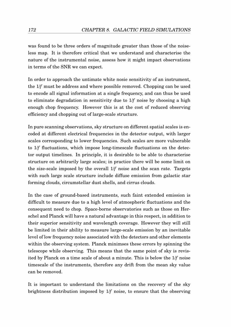
172 CHAPTER 8. GALACTIC FIELD SIMULATIONS
was found to be three orders of magnitude greater than those of the noise-less map. It is therefore critical that we understand and characterise thenature of the instrumental noise, assess how it might impact observationsin terms of the SNR we can expect.
In order to approach the untimate white nosie sensitivity of an instrument,the 1/f must be address and where possible removed. Chopping can be usedto encode all signal information at a single frequency, and can thus be usedto eliminate degradation in sensitivity due to 1/f noise by choosing a highenough chop frequency. However this is at the cost of reduced observingefficiency and chopping out of large-scale structure.
In pure scanning observations, sky structure on different spatial scales is en-coded at different electrical frequencies in the detector output, with largerscales corresponding to lower frequencies. Such scales are more vulnerableto 1/f fluctuations, which impose long-timescale fluctuations on the detec-tor output timelines. In principle, it is desirable to be able to characterisestructure on arbitrarily large scales; in practice there will be some limit onthe size-scale imposed by the overall 1/f noise and the scan rate. Targetswith such large scale structure include diffuse emission from galactic starforming clouds, circumstellar dust shells, and cirrus clouds.
In the case of ground-based instruments, such faint extended emission isdifficult to measure due to a high level of atmospheric fluctuations and theconsequent need to chop. Space-borne observatories such as those on Her-schel and Planck will have a natural advantage in this respect, in addition totheir superior sensitivity and wavelength coverage. However they will stillbe limited in their ability to measure large-scale emission by an inevitablelevel of low frequency noise associated with the detectors and other elementswithin the observing system. Planck minimses these errors by spinning thetelescope while observing. This means that the same point of sky is revis-ited by Planck on a time scale of about a minute. This is below the 1/f noisetimescale of the instruments, therefore any drift from the mean sky valuecan be removed.
It is important to understand the limitations on the recovery of the skybrightness distribution imposed by 1/f noise, to ensure that the observing
173
Noiseless simulation Noisy (1/f) simulationOriginal input map Original input map
Simulation output map Simulation output map
Map residuals (simulated− original) Map residuals (simulated− original)
1
Figure 8.1: Sample noiseless (left) and noisy (right) simulated galactic field obser-vations. Simulated output maps are shown in the middle panals, and the residualsof the input-output maps are shown in the bottom panals. Note, the cut levels infirst four panels have been set such that they show large and small scale structure.Consequently the scale shown does not represent the full range of flux density. Asa result some compact sources are saturated in this image. The brightest source inthe image is ∼10 MJy/sr.
174 CHAPTER 8. GALACTIC FIELD SIMULATIONS
modes and integration times are optimised, and that the analysis methodsto be used are well matched to the data. A thorough understanding of theexpected SNR from an observation of such a diffuse region is also importantin the planning of specific science programmes. This is particularly impor-tant for satellite instruments like SPIRE, for which observing time is costlyand the in-flight time available for performance verification and optimisa-tion is limited. In order to investigate the parameter space influenced bysuch systematics, I have carried out a series of investigations using the SPS.Although some aspects of these simulations are particular to SPIRE, themain results of this analysis will apply to any scanning photometric instru-ment which is limited by uncorrelated 1/f noise.
In this chapter I outline the general source types to be observed within thegalactic SPIRE guaranteed time programmes (SAGs 3, 4, and 6, reviewed inSection 3.3), and identify the key questions relating to instrument system-atics that need to be answered in order to plan these observations efficiently.Following this, I outline a series of simulations performed in order to answersome of these questions, and discuss the results, and their implications forboth the SPIRE programmes, and scanning instruments in general.
8.1 SPIRE Galactic Mapping Programmes
The SPIRE consortium is currently formulating a series of key programmeswhich will include various mapping observations of galactic regions (SAGs3, 4, and 6, reviewed in Section 3.3). These surveys will cover a wide range ofsource types and will be typical of many other expected ‘Open Time’ observ-ing programmes. The varied scientific goals will require accurate recoveryof point-like or compact sources, such as embedded objects and star-formingcores, more extended sources such as circumstellar dust shells and super-nova remnants, and the very extended structure in molecular clouds. Thelatter will pose the greatest challenge for the recovery of large-scale bright-ness structure.
As part of the SAG 3 investigation into the early stages of star formation,
8.1. SPIRE GALACTIC MAPPING PROGRAMMES 175
a census of prestellar condensations and young Class 0 protostars, down toa mass limit of 0.01 M will be made in nearby molecular cloud complexes(Andre and Saraceno, 2005). This information will provide a complete coremass function down to the brown dwarf regime. Accurate recovery of thesesources over the full range of flux levels is essential in order to understandthe mechanisms involved in the earliest stages of star formation, in partic-ular to understanding the origin of the stellar initial mass function (IMF).Current data for the core mass function shows it to have a similar slope tothat of the IMF (Motte et al., 2001; Nutter and Ward-Thompson, 2007), andhence is important in the determination of the early stages of cloud fragmen-tation and collapse.
In addition to the need to extract compact sources, it is also of interest to beable to recover the radial brightness profiles of prestellar cores. This can beused to obtain the density and temperature profiles within the core, provid-ing information to test current core collapse models. The limit to which aradial profile can be accurately recovered, in the presence of 1/f noise, and aconfused environment, is not yet known.
Planning is also underway to map a series of circumstellar dust shells andlarge-scale ISM structure, as well as an analysis of the extragalactic infraredbackground fluctuations. The large angular scale fluctuations associatedwith these targets makes them particularly susceptible to 1/f noise, and thispresents a tough observing challenge.
It will be important in the case of these, and similar surveys, that the goals ofboth large scale structure and compact source science cases can be achievedin a single set of observations. It is therefore essential to establish the im-pact of telescope and instrument systematics on each case and optimise thefinal observing strategy accordingly. To this end I have identified the fol-lowing set of key questions relating specifically to the observation of galactictargets:
1. What are the limitations and effects of 1/f noise on the accuracy ofrecovery of large-scale structure?
2. How does the simultaneous presence of 1/f noise and diffuse cirrus
176 CHAPTER 8. GALACTIC FIELD SIMULATIONS
limit the detection of compact sources?
3. What is the impact of 1/f noise on our ability to reconstruct the radialprofiles of compact cores?
8.2 Simulations
A series of simulations was performed in order to address the questions setout above. The initial set of simulations was aimed at answering the firstquestion: to assess, in a general way, the effect of 1/f noise on the abil-ity to recover structure of an arbitrary scale. These simulations were firstperformed in a simple one dimensional case, followed by a more realistic2D study of simple Gaussian sources. The next stage dealt with noise-onlymaps, which represent a real life observing situation with no prior source in-formation. These results were then applied to the case of compact sources inthe presence of a diffuse cirrus cloud structure, in order to address the sec-ond key question. A final set of simulated observations, was then created,and the recovery of an input radial core profile assessed. These simulationstackle the last key question.
The SPIRE scan-map mode without chopping (POF 5, see Section 3.2) wasused for all simulations. In order to establish the fundamental limits on dataquality imposed by unavoidable 1/f noise from the detectors themselves, var-ious simplifications were introduced: no common mode noise or pointing er-rors were included; the detectors in a given array were taken to be identical(perfect flat-fielding); and there were no correlated thermal drifts, cross-talkor glitches. Whilst these conditions are not fully representative of the realsystem performance, they do allow us to investigate the consequence of 1/fnoise alone. Other noise effects may also reduce the data quality, but thesewill act as a scaling upon the results presented here.
The noise timeline imposed on each detector was unique, but generated us-ing the same noise spectrum (noise voltage spectral density, en, and 1/f noiseknee frequency, fk). This represents uncorrelated noise within each detectorchannel arising from independent detectors and their readouts.
8.2. SIMULATIONS 177
The simulated time ordered data were converted to a map using a simple fluxbinning method to produce a ‘naıve’ map. This method assigns a value to amap pixel equal to the mean value of all data counts falling within that pixel(see Section 5.3). This was used to provide a baseline result, against whichthe improvement resulting from more sophisticated data analysis methodscould be compared.
To quantify the effect of 1/f noise, the achieved SNR for a source in thepresence of 1/f noise is quoted as a fraction of the SNR from an equivalentwhite noise observation. This is referred to as the SNR loss factor (SNRlf )and is given in Equation 8.1. This method of evaluation is like that used inChapter 6.
SNR loss factor =SNR1/f
SNRwhite
, (8.1)
where SNR1/f is the SNR in an observation containing 1/f noise, and SNRwhite
is the SNR of the same observation in the white noise case. This allows usto quantify the sensitivity degradation due to 1/f noise, independent of theintegration time and source flux density.
The degradation of SNR in the presence of 1/f depends on the 1/f noise kneefrequency, fk, the telescope scan rate, θ, and the beam-convolved source sizescale, λ. Together, fk and θ determine the spatial frequency scale in the mapcorresponding to the 1/f knee frequency (fs = fk/θ). The equivalent angularsize scale is λs = 1/fs. Crudely, the SNR of a source close to or greater thanthis scale, observed in the presence of 1/f noise, will be significantly reduced.
It is convenient to define a new variable, ψ, in the following way:
ψ =fk
θ
√λ. (8.2)
This combines all the information from the three related variables into asingle parameter. The impact of 1/f noise is influenced by all three param-eters and identical results can be achieved for a range of source scales andscan rates for a given 1/f noise knee frequency. A single scalable plot canbe derived which is capable of representing any combination of the depen-dent parameters. The form of Equation 8.2 is explained in Section 8.4 below,in which a general analysis is presented (applicable to any scanning instru-
178 CHAPTER 8. GALACTIC FIELD SIMULATIONS
ment which is affected by uncorrelated 1/f noise). In this analysis, the sensi-tivity is characterised as a function of the parameter ψ, and the results canbe used to determine the effective sensitivity as a function of any one of thekey parameters, keeping the other parameters constant.
8.2.1 1D Simulations
In order to characterise the influence of 1/f noise on observations of large-scale structure in the most general case, an initial simple one dimensionalstudy was performed. Here a single detector was scanned once across a1D Gaussian source characterised by its width and brightness. A 1/f noisetimeline was then added to the resulting detector voltage time series. ThreeGaussian source sizes were explored varying from a beam convolved widthequal to 1, 1.5, and 2.0 times the beam FWHM. The SPIRE 250 µm bandwith a size of 16.2′′ was used for this study, but the results can be param-eterised in a straightforward way to an arbitrary beam size (see Equation8.2).
For computational convenience, the scan rate was kept constant at 25′′s−1,and a range of 1/f knee frequencies from 0 Hz (white) to 2 Hz was explored.Five hundred simulations were performed for each value of fk, and a Gaus-sian fit made to each. For the amplitude of the Gaussian, the ideal (noise-less) result is for the fitted amplitude to be equal to the amplitude of thebeam-convolved source. The reciprocal of the standard deviation of the in-put:output amplitude ratio from unity is adopted as a measure of the SNR.
In addition to a variety of knee frequencies and source sizes, various baselinelengths were also used in the fitting of the Gaussian curve. Thus an optimumbaseline was found for a given value of fk.
8.2.2 2D Simulations
The 1-D simulations were then extended to the case of two dimensionalmaps. As with the 1-D case, the input skies used in the simulations were
8.2. SIMULATIONS 179
a set of simple 2D ‘toy’ skies containing isolated Gaussian sources of varyingfull width half maximum (FWHM) with zero background. A range of Gaus-sian sources with beam-convolved sizes up to 10 beam FWHM was used.These represent astronomical signals spanning a range of spatial scales, andallowed for a straightforward evaluation of the ability of any scanning sys-tem to extract extended source structure in the presence of 1/f noise. Thesimplicity of this input sky provides a representative general result applica-ble to all science cases.
Five hundred maps were again created for each λ and fk combination. Thedata from each detector time series were then used to produce a naıve mapas described in Chapter 5. The same assessment of the data as in the 1-Dcase was carried out, this time fitting a Gaussian surface.
8.2.3 Noise Map Simulations
Next, a series of tests was performed using a blank input sky. Noise mapswere produced with a range of pixel sizes. The reciprocal of the standarddeviation of the map pixels was then taken as the SNR for sources of thatpixel size. This was then compared with the white noise case to obtain aSNR loss factor as before.
To make this analysis equivalent to the 2D case above, the source scale,defined by the map pixel size, must be scaled by a factor of 1/
√2. This results
in a scale size which contains 1/2 of the total pixel flux, equivalent to theFWHM scaling used in the 2D case.
8.2.4 Radial Profile Simulations
Finally, the SPS was used to simulate eight observations of a synthetic sky,populated with 36 critical BESs (Section 2.3.3), with a FWHM size of 5 PSWbeams. Two scans were performed for each simulation with perpendicularscan angles, as defined in Chapter 6. Each simulation contained a differentvalue of fk, ranging from 0 (white) to 2 Hz (severe 1/f ).
180 CHAPTER 8. GALACTIC FIELD SIMULATIONS
It is likely that cores with a wide range of widths will be observed, frompoint-like to many beams in scale. The width of the spheres used in thesesimulations is representative of a realistic BES located at the distance of theOrion nebula.
The radial profile extraction routine ‘ELPROF’ by Currie and Berry (2001)was used to construct the radial profiles from the simulated output maps.The program bins the pixels in a map into a series of concentric ellipticalor circular annuli. The mean pixel value in each annulus is then returned,giving the radial profile. It was assumed that the source location was knownperfectly, and that the source was circular.
A χ2 test, used to measure how well a particular hypothesis matches thedata, in this case how well the radial profile data match the input model,was used to assess the results. The χ2 statistic with k free parameters hasthe following distribution,
χ2 =k∑i=0
(Xi − µiσi
)2
, (8.3)
where Xi are the data, µi is the mean value of Xi, and σ is the standarddeviation of the data. A certain value of the reduced χ2 relates to a specificprobability that the data match the model, given a certain number of freeparameters (measurements).
The output χ2 values were normalised with respect to the white noise case,and a χ2 gain factor, χ2
gf , was deduced for each value of fk. This is the factorby which χ2 is increased with respect to χ2 value obtained in an observationcontaining only white noise.
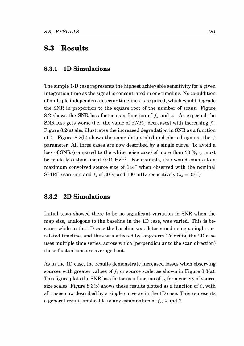
8.3. RESULTS 181
8.3 Results
8.3.1 1D Simulations
The simple 1-D case represents the highest achievable sensitivity for a givenintegration time as the signal is concentrated in one timeline. No co-additionof multiple independent detector timelines is required, which would degradethe SNR in proportion to the square root of the number of scans. Figure8.2 shows the SNR loss factor as a function of fk and ψ. As expected theSNR loss gets worse (i.e. the value of SNRlf decreases) with increasing fk.Figure 8.2(a) also illustrates the increased degradation in SNR as a functionof λ. Figure 8.2(b) shows the same data scaled and plotted against the ψ
parameter. All three cases are now described by a single curve. To avoid aloss of SNR (compared to the white noise case) of more than 30 %, ψ mustbe made less than about 0.04 Hz1/2. For example, this would equate to amaximum convolved source size of 144′′ when observed with the nominalSPIRE scan rate and fk of 30′′/s and 100 mHz respectively (λs = 300′′).
8.3.2 2D Simulations
Initial tests showed there to be no significant variation in SNR when themap size, analogous to the baseline in the 1D case, was varied. This is be-cause while in the 1D case the baseline was determined using a single cor-related timeline, and thus was affected by long-term 1/f drifts, the 2D caseuses multiple time series, across which (perpendicular to the scan direction)these fluctuations are averaged out.
As in the 1D case, the results demonstrate increased losses when observingsources with greater values of fk or source scale, as shown in Figure 8.3(a).This figure plots the SNR loss factor as a function of fk for a variety of sourcesize scales. Figure 8.3(b) shows these results plotted as a function of ψ, withall cases now described by a single curve as in the 1D case. This representsa general result, applicable to any combination of fk, λ and θ.
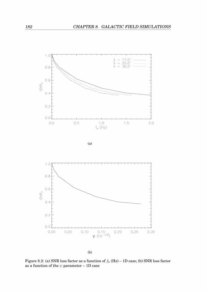
182 CHAPTER 8. GALACTIC FIELD SIMULATIONS
(a)
(b)
Figure 8.2: (a) SNR loss factor as a function of fk (Hz) – 1D case; (b) SNR loss factoras a function of the ψ parameter – 1D case
8.3. RESULTS 183
(a)
(b)
Figure 8.3: (a) SNR loss factor as a function of fk for a variety of source size scales,with a fixed scan rate of 30′′/s; (b) SNR loss factor as a function of ψ.
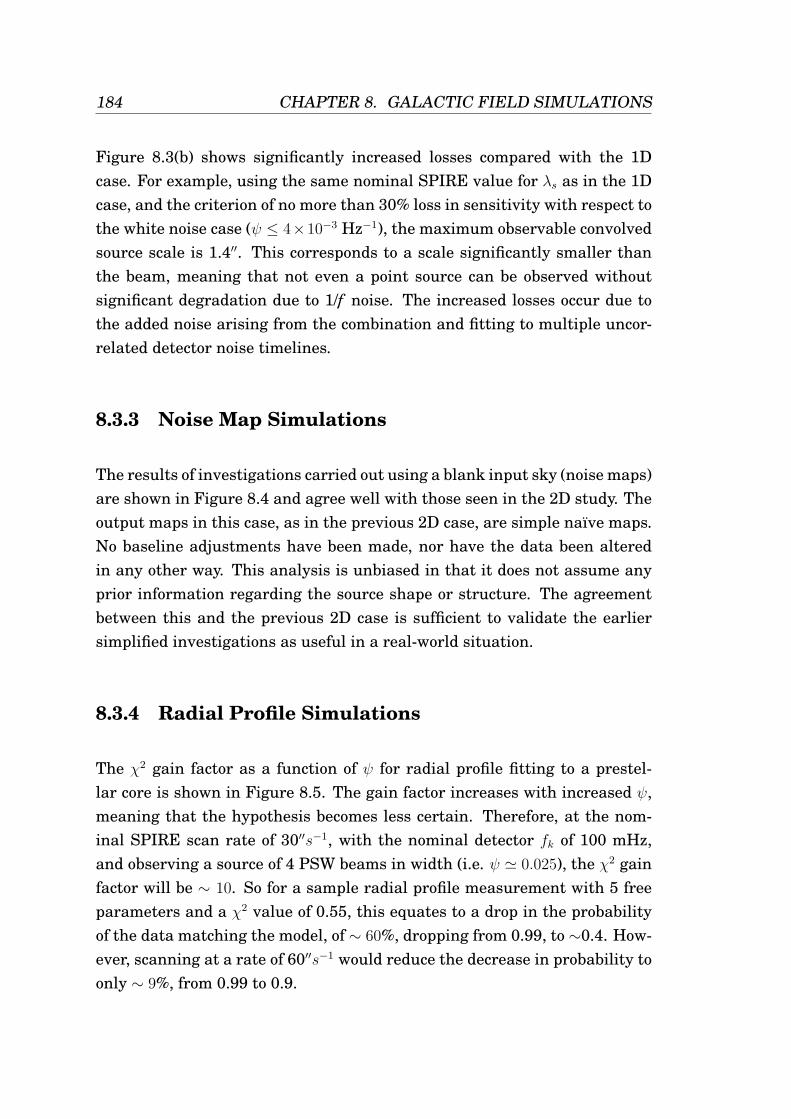
184 CHAPTER 8. GALACTIC FIELD SIMULATIONS
Figure 8.3(b) shows significantly increased losses compared with the 1Dcase. For example, using the same nominal SPIRE value for λs as in the 1Dcase, and the criterion of no more than 30% loss in sensitivity with respect tothe white noise case (ψ ≤ 4×10⁻³ Hz−1), the maximum observable convolvedsource scale is 1.4′′. This corresponds to a scale significantly smaller thanthe beam, meaning that not even a point source can be observed withoutsignificant degradation due to 1/f noise. The increased losses occur due tothe added noise arising from the combination and fitting to multiple uncor-related detector noise timelines.
8.3.3 Noise Map Simulations
The results of investigations carried out using a blank input sky (noise maps)are shown in Figure 8.4 and agree well with those seen in the 2D study. Theoutput maps in this case, as in the previous 2D case, are simple naıve maps.No baseline adjustments have been made, nor have the data been alteredin any other way. This analysis is unbiased in that it does not assume anyprior information regarding the source shape or structure. The agreementbetween this and the previous 2D case is sufficient to validate the earliersimplified investigations as useful in a real-world situation.
8.3.4 Radial Profile Simulations
The χ2 gain factor as a function of ψ for radial profile fitting to a prestel-lar core is shown in Figure 8.5. The gain factor increases with increased ψ,meaning that the hypothesis becomes less certain. Therefore, at the nom-inal SPIRE scan rate of 30′′s−1, with the nominal detector fk of 100 mHz,and observing a source of 4 PSW beams in width (i.e. ψ ' 0.025), the χ2 gainfactor will be ∼ 10. So for a sample radial profile measurement with 5 freeparameters and a χ2 value of 0.55, this equates to a drop in the probabilityof the data matching the model, of ∼ 60%, dropping from 0.99, to ∼0.4. How-ever, scanning at a rate of 60′′s−1 would reduce the decrease in probability toonly ∼ 9%, from 0.99 to 0.9.
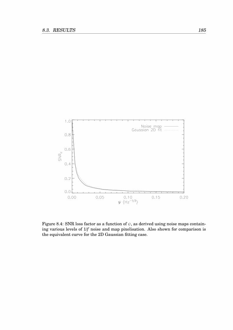
8.3. RESULTS 185
Figure 8.4: SNR loss factor as a function of ψ, as derived using noise maps contain-ing various levels of 1/f noise and map pixelisation. Also shown for comparison isthe equivalent curve for the 2D Gaussian fitting case.
186 CHAPTER 8. GALACTIC FIELD SIMULATIONS
Figure 8.5: χ2 gain factor as a function of ψ, for radial profile fitting to a prestellarcore. In this specific case the model used was a critical BES.
8.4. DISCUSSION 187
8.4 Discussion
8.4.1 Large Scale Structure
A series of many simulations was used to derive the noise level in the abovetests requiring many repeat observations of the source. This is generallynot possible in real life, and in many cases the noise is simply derived fromthe standard deviation of some empty region of the map, and assumed to beconstant throughout. However, this method is only applicable in the pres-ence of white noise. Also, in doing this it is implicitly assumed that there isno dependence of SNRlf with source scale, which is not true. Correlationswithin the 1/f noise result in the
√λ dependence seen in Equation 8.2. Any
form of correlation (including those introduced in many instruments by on-board filters) will result in a source size dependence, and will generally causean over-estimate of the SNR. An example of this can be seen in Figure 8.6,which shows SNRlf curves derived using the above Monte Carlo Gaussianfitting method, and from the matched filtering method described in Chapter5, which assumes white noise. The matched filtering method uses knowl-edge of the source shape in order to weight the data, and thus derive theoptimal SNR. These curves were generated using the data set from the 2Dstudy above. The figure contains four curves, representing different sourcescales, for each method. The overlap of the curves in the matched filteringcase demonstrates the apparent, and erroneous scale independence of thewhite noise assumption method.
The increased losses in SNR seen in the 2D cases over the 1D case are large;however it is possible to improve significantly on these losses by applyingvarious data reduction methods during the map-making stages. Adjust-ments can be made in an attempt to reduce the effects of 1/f noise drifts,such as median filtering, high-pass filtering, and baseline subtraction. Allsuch filtering methods destroy some information in their implementation,and require assumptions to be made regarding the maximum source scalepresent in the data. Consequently these methods are of limited use whenmeasuring large-scale structure, but they can be effective when the targetsource is known to be point-like or small, i.e. a source with relatively little
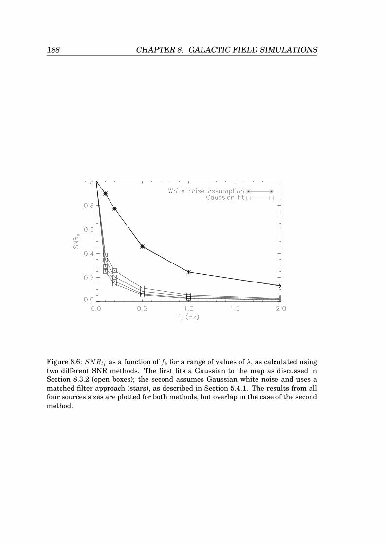
188 CHAPTER 8. GALACTIC FIELD SIMULATIONS
Figure 8.6: SNRlf as a function of fk for a range of values of λ, as calculated usingtwo different SNR methods. The first fits a Gaussian to the map as discussed inSection 8.3.2 (open boxes); the second assumes Gaussian white noise and uses amatched filter approach (stars), as described in Section 5.4.1. The results from allfour sources sizes are plotted for both methods, but overlap in the case of the secondmethod.
8.4. DISCUSSION 189
low frequency structure (Haig et al., 2004; Waskett et al., 2006). Examplesof naıve maps, and the equivalent high-pass filtered maps are shown in Fig-ures 8.7 and 8.8. The degradation in the peak signal can be seen in thefiltered maps in comparison with that of the naıve maps.
Another technique to reduce the effects of 1/f noise is based on establishingthe power spectrum of the 1/f noise within an observation. This informationis then used to estimate and remove the noise correlations in the output map(see Section 5.3). This method is widely used by cosmic microwave back-ground (CMB) experimenters (Poutanen et al., 2006; Tegmark, 1997), whoare interested in a wide range of scales on the sky. It produces a maximumlikelihood map and does not require any prior assumptions about the data.This method also does not result in the ringing artefacts, often seen whenusing the previous filtering techniques.
Both approaches are often used in data reduction. In order to assess therelative improvement presented by each method, the 2D tests were repeatedusing high-pass filtered, and maximum likelihood maps as inputs.
A high-pass filter with a four PSW beam (∼65′′) cut-off was applied to thetime ordered data, filtering the data in the scan direction. The maximumlikelihood maps were generated by directly solving the generalised leastsquares formula, Equation 5.3 (Section 5.3). In order to employ this methoda cross-linked observation is required. The performance of this method isa function of the scan pattern implemented; a greater level of cross-linkingwill improve its ability to remove 1/f drifts. In these simulations, two per-pendicular Boustrophedon scan patterns were implemented (Figure 3.8). Asmall 30 × 30 pixel map was produced using one detector for computationalefficiency. The corresponding data redundancy is representative of the typi-cal level of cross-linking available when observing with an observatory suchas Herschel, which does not have scope for complicated scanning patternsdue to telescope control limitations. As before, the noise was kept station-ary for these tests. A model noise covariance matrix was derived from themean of many independently generated matrices. An inferior noise covari-ance matrix will result in a greater rate of SNR loss with increasing ψ. Thismay occur if there are limited data from which to derive the matrix. Con-
190 CHAPTER 8. GALACTIC FIELD SIMULATIONS
versely, greater cross-linking within the observation may reduce the rate ofSNR loss with increasing ψ. The result presented by this analysis shows theimprovement in data quality achieved with this method, even in this simpleexample. Examples of the maps produced by both methods are shown, incomparison with their naıve map equivalents, containing various levels offk, in Figures 8.7, 8.8, 8.9 and 8.10.
The results from these treatments of the data, along with the naıve 2D caseare shown in a generalised plot in Figure 8.11. In addition, the 1D result isshown for comparison. The maximum likelihood results are clearly superiorto both the naıve and filtered cases.
Using again the criterion of no more than 30% loss of sensitivity with respectto the white noise case, and a λs of 300′′, the maximum convolved source sizescales for the naıve, filtered, and maximum likelihood maps are 1.4′′, 9′′, and110′′ respectively. It should be noted that any frequency dependent systemcomponent, such as a filter, must be considered in conjunction with theseresults. Some systems for example include a high-pass filter, which willsuppress both 1/f noise and large scale signals. In this case these resultswill be less applicable.
8.4.2 Limiting Source Flux in a Confused Environment
Every astronomical survey has a limiting sensitivity, below which sourcescannot be readily identified. This limiting sensitivity relates to a limitingSNR within the map. Often this level is set with respect to the confusionnoise (see Section 2.4.3) level within the region; e.g., for a survey with aminimum source detection threshold of 10σ, the limiting SNR would be 10times the confusion noise level. In practice however, it is not possible toreach this level as there will always be some residual instrumental noisein the data. The results from Section 8.4.1 have been used to investigatethe limiting SNR achievable with a survey, given a range of fk, θ, λ, andconfusion noise level (σconf ) parameters.
Initially, the limiting flux was derived for a white noise survey over a range
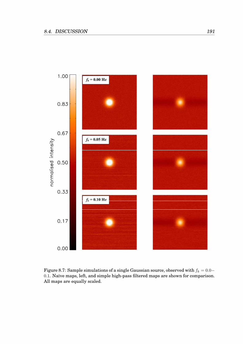
8.4. DISCUSSION 191
Figure 8.7: Sample simulations of a single Gaussian source, observed with fk = 0.0−0.1. Naıve maps, left, and simple high-pass filtered maps are shown for comparison.All maps are equally scaled.
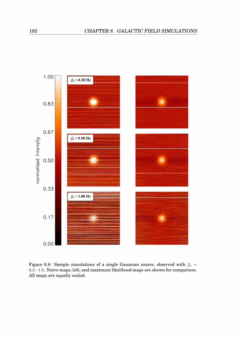
192 CHAPTER 8. GALACTIC FIELD SIMULATIONS
Figure 8.8: Sample simulations of a single Gaussian source, observed with fk =0.2−1.0. Naıve maps, left, and maximum likelihood maps are shown for comparison.All maps are equally scaled.
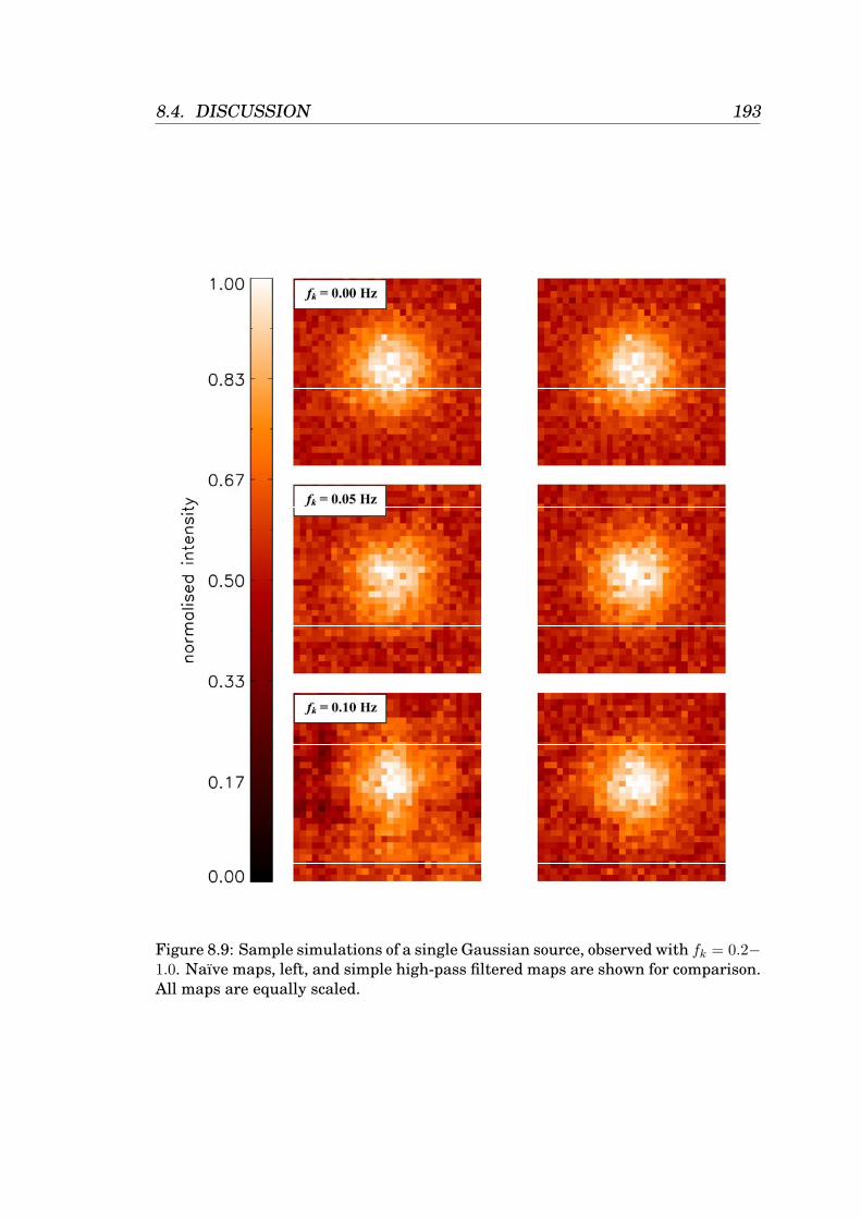
8.4. DISCUSSION 193
Figure 8.9: Sample simulations of a single Gaussian source, observed with fk = 0.2−1.0. Naıve maps, left, and simple high-pass filtered maps are shown for comparison.All maps are equally scaled.
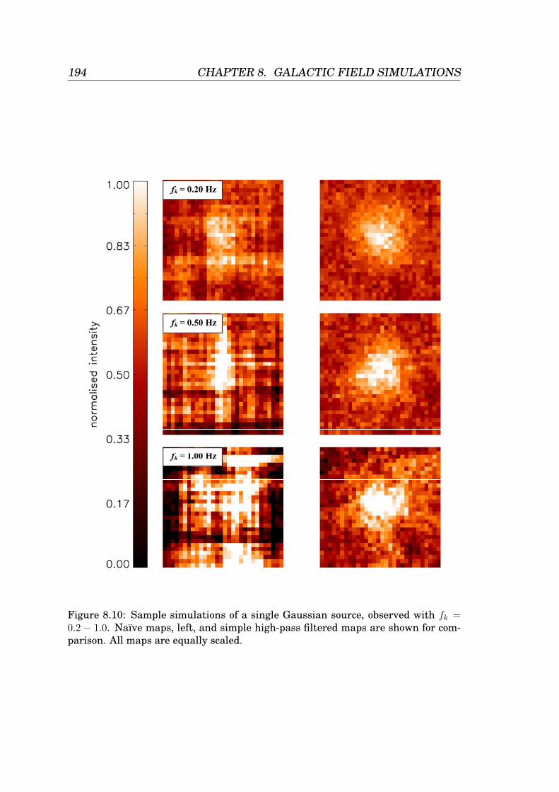
194 CHAPTER 8. GALACTIC FIELD SIMULATIONS
Figure 8.10: Sample simulations of a single Gaussian source, observed with fk =0.2 − 1.0. Naıve maps, left, and simple high-pass filtered maps are shown for com-parison. All maps are equally scaled.
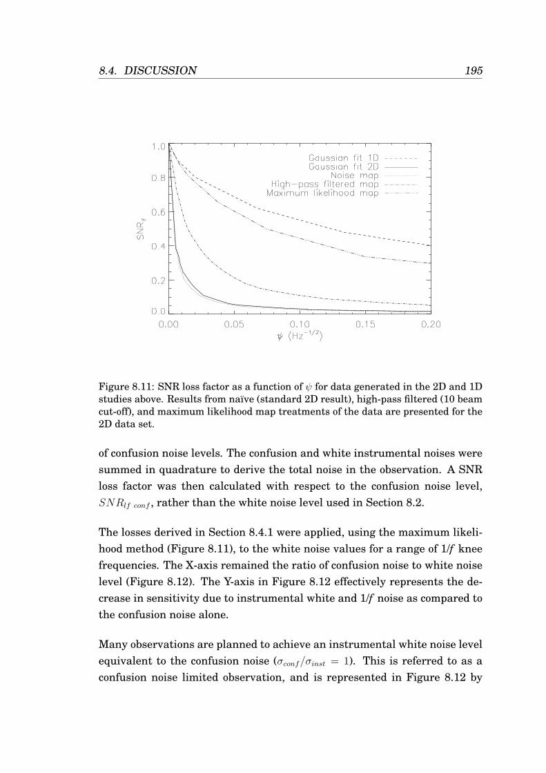
8.4. DISCUSSION 195
Figure 8.11: SNR loss factor as a function of ψ for data generated in the 2D and 1Dstudies above. Results from naıve (standard 2D result), high-pass filtered (10 beamcut-off), and maximum likelihood map treatments of the data are presented for the2D data set.
of confusion noise levels. The confusion and white instrumental noises weresummed in quadrature to derive the total noise in the observation. A SNRloss factor was then calculated with respect to the confusion noise level,SNRlf conf , rather than the white noise level used in Section 8.2.
The losses derived in Section 8.4.1 were applied, using the maximum likeli-hood method (Figure 8.11), to the white noise values for a range of 1/f kneefrequencies. The X-axis remained the ratio of confusion noise to white noiselevel (Figure 8.12). The Y-axis in Figure 8.12 effectively represents the de-crease in sensitivity due to instrumental white and 1/f noise as compared tothe confusion noise alone.
Many observations are planned to achieve an instrumental white noise levelequivalent to the confusion noise (σconf/σinst = 1). This is referred to as aconfusion noise limited observation, and is represented in Figure 8.12 by
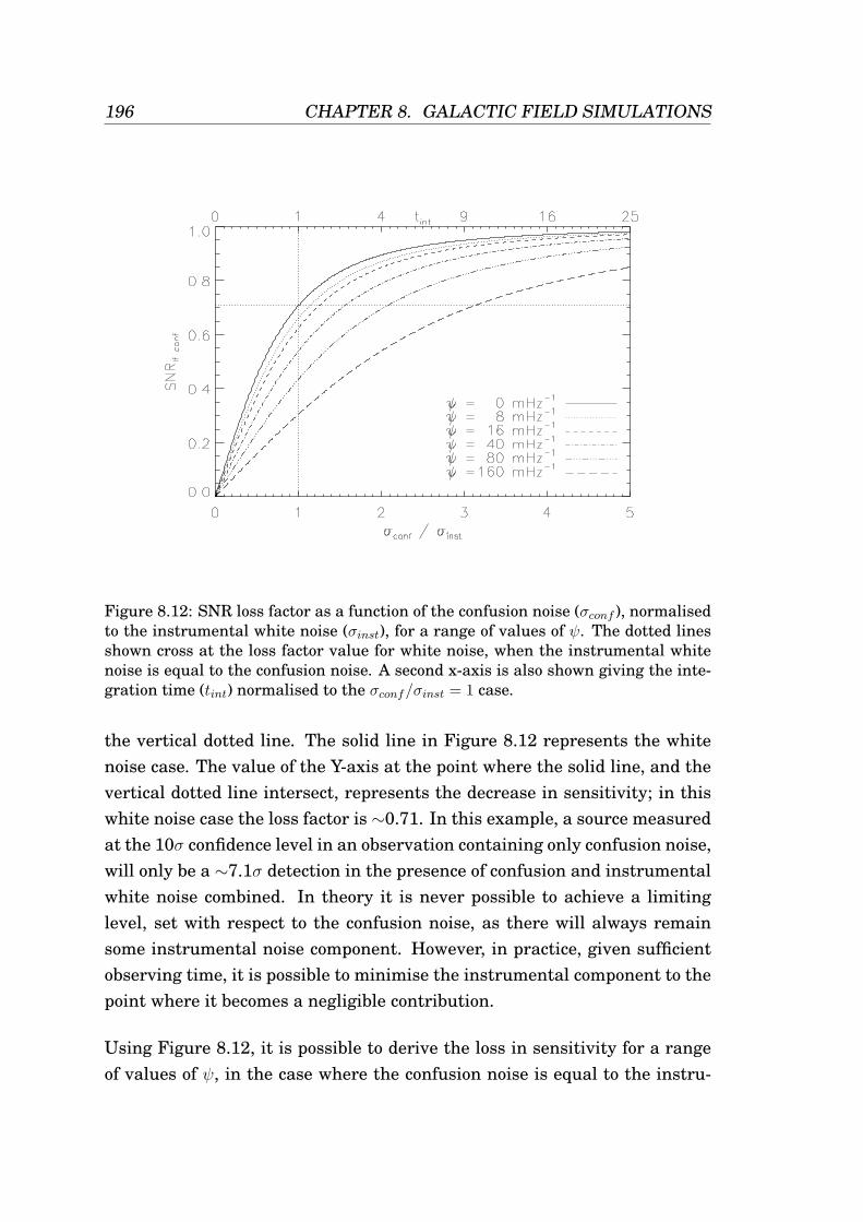
196 CHAPTER 8. GALACTIC FIELD SIMULATIONS
Figure 8.12: SNR loss factor as a function of the confusion noise (σconf ), normalisedto the instrumental white noise (σinst), for a range of values of ψ. The dotted linesshown cross at the loss factor value for white noise, when the instrumental whitenoise is equal to the confusion noise. A second x-axis is also shown giving the inte-gration time (tint) normalised to the σconf/σinst = 1 case.
the vertical dotted line. The solid line in Figure 8.12 represents the whitenoise case. The value of the Y-axis at the point where the solid line, and thevertical dotted line intersect, represents the decrease in sensitivity; in thiswhite noise case the loss factor is ∼0.71. In this example, a source measuredat the 10σ confidence level in an observation containing only confusion noise,will only be a ∼7.1σ detection in the presence of confusion and instrumentalwhite noise combined. In theory it is never possible to achieve a limitinglevel, set with respect to the confusion noise, as there will always remainsome instrumental noise component. However, in practice, given sufficientobserving time, it is possible to minimise the instrumental component to thepoint where it becomes a negligible contribution.
Using Figure 8.12, it is possible to derive the loss in sensitivity for a rangeof values of ψ, in the case where the confusion noise is equal to the instru-
8.4. DISCUSSION 197
mental white noise (σconf/σinst = 1). This is done by inspecting the value ofthe y-axis where the line associated with a particular value of ψ, intersectsthe dotted vertical line. For example, by locating where the ψ = 80 mHz−1/2
curve meets the vertical dotted line, we can obtain the sensitivity degrada-tion for that value of ψ – in this case the detection significance would fall to0.4 of that which might be achieved in a confusion noise only observation.Thus, for a 10σ limit defined with respect to the confusion noise level, thefinal detection would actually be 4σ.
In order to achieve a detection limit equivalent to that of the white noisecase, in the presence of 1/f noise, an increased integration time will be re-quired to lower the instrumental noise level. This can be quantified by lo-cating the point at which the curve of interest crosses the horizontal dottedline, and reading off the value on the upper X-axis. Taking again as an ex-ample the case of ψ = 80 mHz−1/2, to achieve a SNRlf conf equivalent to thatof the white noise case (∼ 0.71) the integration time must be increased byapproximately a factor of four.
The improvement in limiting SNR resulting from faster scanning can alsobe easily derived from this figure. Doubling the scanning rate will halvethe value of ψ for a fixed λ and fk due to the inverse relation of ψ with θ
(Equation 8.2). Consequently the loss factor would improve from 0.4 to 0.53when the confusion to instrumental white noise level ratio is equal to unity.Also, the extra integration time required to achieve the equivalent detectionlimit to that of a white noise observation would decrease from a factor of ∼4to ∼3.
8.4.3 Radial Profile Fitting
The data in Figure 8.5 demonstrate that, as is the case with the other tests,the data quality rapidly degrades with increased values of ψ. Therefore, ourability to ascertain the correct radial profile and fit it to a specific modelis affected equivalently. The rapid increase in gain factor at low values ofψ (∼0.02) means that high scanning rates are preferable, giving an overallfactorial improvement in χ2 of 2.2 when scanning at 60′′s−1 as opposed to
198 CHAPTER 8. GALACTIC FIELD SIMULATIONS
30′′s−1. Since any source for which a radial profile is being sought must begreater than the beam size, the signal response, even at a high scan rate,will not approach the low-pass filter cut off, and so will not impose a limitingfactor in the case of SPIRE. Therefore, the fastest scanning rate possibleis advised. However, this must be balanced with the increased overheadsassociated with a fast scanning rate, in order to derive the optimal observingstrategy.
The test performed here used naıve maps only. It is reasonable to expect theχ2 gain factor to be reduced by a similar factor to that seen in the large scalestructure tests. Until a maximum likelihood map-maker capable of dealingwith full scale simulations is available, however, it will not be possible to testthis supposition. For now these results can be used as a worst case scenario,i.e. an upper limit to the χ2 gain factor for a specific value of ψ.
The results of these tests focus on the extraction of prestellar cores, but arehowever applicable to observations of nearby galaxies too. Similar methodsare employed to determine the luminosity profiles of galaxies, in order todetermine their morphology.
8.5 Chapter Summary
This chapter has described a series of investigations of the impact of uncor-related 1/f noise when observing with a DC coupled scanning instrument,as a function of 1/f knee frequency, scanning rate, and convolved source sizescale. The results represent the realistic limits to the sensitivity of a scan-ning instrument when observing sources of an arbitrary scale. While thereare many other possible systematic effects, it is likely that these will actmerely as a scaling on the normalised SNR, or can be modelled indepen-dently and considered in conjunction with these results. High-pass filteredand maximum likelihood maps were generated in order to provide a realisticexample of how the data might be treated, and to assess how these methodscan reduce the degradation in sensitivity caused by 1/f noise.
8.5. CHAPTER SUMMARY 199
The losses due to 1/f noise were found to increase linearly with knee fre-quency, as the square root of convolved source size scale, and inversely withscanning rate. A parameterisation of these three variables was presented(see Equation 8.2) in order to provide a curve which is scalable to a generalsystem using any combination of these factors. Generation of a maximumlikelihood map was found to significantly reduce the impact of 1/f noise com-pared with a naıve approach or high-pass filtering.
The results from this investigation were also applied to the case of a confusedobservation in order to ascertain the impact of 1/f noise on the accuratedetermination of the detection level within a survey. It was found that anincrease in scanning rate can substantially reduce the added integrationtime required to overcome the degradation due to 1/f noise. However, theanti-aliasing filter contained within most real-life systems will degrade anysignal beyond its cut-off frequency. The improvement resulting from a highscan rate must be coupled with the losses experienced due to the filter. Inaddition, operational constraints such as telescope overheads may limit thescan rate.
The final test performed analysed how telescope scan rate, 1/f noise kneefrequency, and source size scale, affect our ability to recover, and identify,the radial profile of a prestellar core. They show that in general, the qualityof the fit degrades quickly at low values of ψ. However, a high scan ratewill result in a decreased value of ψ, which corresponds to a significant im-provement to the χ2 value, and therefore a more confident correlation with aspecific model.
The results outlined are important in the planning of large scale observingprogrammes in which both extended and compact sources are required to beobserved simultaneously. They allow for an informed selection of scanningstrategy to ensure that the source scales of interest are observed efficiently.They also provide information on the integration times required to ensurethat the desired detection limits are reached.
This study also illustrates how the often used method of determining noisein a map, by measuring the pixel-to-pixel standard deviation within a blankregion of the map, is misleading when dealing with correlated noise. The

200 CHAPTER 8. GALACTIC FIELD SIMULATIONS
invalid assumption of scale invariance will result in an incorrect determina-tion of SNR, and its dependence on size scale in the map.
Chapter 9
Conclusions and Future Work
This thesis has focused on the development of a sophisticated Herschel-SPIRE software instrument simulator, and its use in the investigation ofinstrumental effects on observational data in the FIR-submm. Of particularinterest was the optimisation of the SPIRE observing modes and observa-tions of galactic sources, specifically the recovery of structure on arbitraryscales. It has also included analysis of observations of the Cas A SNR madeusing BLAST, with the aim of determining if SNe are a significant source ofdust production in the universe.
Chapter one introduced and summarised FIR/submm astronomy, and thetechniques by which it is performed. Overviews of the Herschel and BLASTprojects were also given, including details of the PACS and HIFI instru-ments on board Herschel. Finally, a qualitative review of bolometer opera-tion was presented.
The following chapter reviewed a range of processes in which dust plays amajor role in the ISM. It highlighted the important role played by cosmicdust, from chemical processing, to the formation of stars, as well as the cyclethrough which dust passes, from birth to destruction. Particular attentionwas paid to a review of the accepted dust formation mechanism in the uni-verse – formation in the atmospheres of evolved (AGB) stars. The overallinjection rates were then compared with those required to generate the dust
201
202 CHAPTER 9. CONCLUSIONS AND FUTURE WORK
fraction seen in the galaxy today. This identified a deficit in the overall pro-duction rate of dust from stars, meaning that another source of dust must befound to explain the observed levels. The need for a new mechanism of dustformation is further supported by the detection of dusty galaxies in the earlyuniverse. This dust could not have been formed by AGB stars, as they wouldnot have had time to reach the necessary evolutionary stage. The currentevidence for SNe as the missing source was then introduced.
A summary of the SPIRE instrument was presented in chapter three. Thisincluded a review of the instrument hardware, observing modes, and sci-entific capabilities, illustrated by a description of the SPIRE consortium’sproposed guaranteed time science programmes.
Chapter four described the SPIRE photometer software simulator, and out-lined its primary goals and operation. The SPS is a highly realistic softwaremodel of the SPIRE photometer, which contains all of the primary photome-ter subsystems. It is capable of simulating the photometer system operation,and data characteristics. The system contains models of each subsystem,to varying levels of sophistication. A brief description of the methods usedto model each instrument subsystem, implemented in the form of a module,has also been presented. The limitations of the simulations have been noted,specifically, that results from simulation can only be representative, and notidentical to, the final system output. This makes the simulator useful in un-derstanding the impact of the known systematics on the data quality, but itcannot predict the final instrument performance until the system is in orbit.
The issue of processing instrument data from raw timelines, to a useable for-mat for astronomy, in this case a map, was addressed in Chapter five. Thevarious data cleaning processes, including removal of cosmic ray detections,correlated noise, and flat-fielding were discussed, and where necessary, anexplanation of these methods, as applied to SPS data, was given. The issuesinvolved with making maps from the processed data were also described,including an explanation of naıve map making, and an overview of the max-imum likelihood map-making method. This method deals with the removalof uncorrelated 1/f noise, and is used widely in studies of the CMB.
This chapter also provided an account of the validation of the SPS signal
203
and noise output. This validation was performed by comparing the SNR ofa point source, observed in scan-map mode, with the theoretical SNR ex-pected. This used data in the form of a naıve map, generated by unfiltereddetector data. The NEFD obtained in this verification exercise was com-pared to the official SPIRE sensitivity model (Griffin, 2004), and found toagree to within ∼ 2%. Finally, an overview of the SPIRE map-making rou-tine selection process was presented, and the reasons for selecting MADmapas the best routine explained.
In Chapter six, the main observing modes for the SPIRE photometer wereassessed, and the baseline optimum parameters derived. POF 2 (7-pointmapping) will be used as the nominal point source photometry mode, with ajiggle position spacing, ∆θ7, of 6′′. This mode is chosen over a single point-ing observation (POF 1) as it guarantees source flux and position recovery,within the Herschel pointing accuracy and reasonable source position errors,with only a small reduction in SNR.
The optimum spacing required within the jiggle map pattern, in order tofully sample all arrays, is 8.1′′. The best spacings between consecutive jig-gle maps when raster mapping, was found to be 245, and 236′′ in the Z andY telescope coordinates respectively. This ensures that the observation re-mains fully sampled at the join between jiggle maps, and that the distribu-tion of integration time remains even.
The optimum scan map mode parameters were found to be a scan rate of30′′s−1, and scan angle of 12.4. Perpendicular scans in the diagonal direc-tions are optimal for large maps, as provide cross-linked data, suitable foruse with a maximum likelihood map-maker. Small and irregular maps how-ever are more efficiently performed by scanning along the long axis. Theoptimum scan line separation for the diagonal and long axis scan directionsare 235 and 348′′ respectively. These parameters minimise the losses dueto 1/f noise and low pass filter systematics, provide full sampling down to14
FWHM, and provide a uniform distribution of integration time across themap.
Scan map mode was found to be more efficient than raster mapping for mapsgreater than 4′ × 4′. In addition to the shorter total observation time, it
204 CHAPTER 9. CONCLUSIONS AND FUTURE WORK
provides a more uniform integration time map, as well as significant bonusdata in the surrounding map regions. As a result this is currently the nomi-nal mode for all but single field jiggle maps (4′ × 4′). Note that this result isnow being reassessed due to new information regarding telescope movementoverheads.
The optimum observing parameters for each of the SPIRE observing modesare summarised in Table 6.2. Specific science cases may require a varia-tion on some parameters, however these nominal values will be used for themajority of observations.
Many of the conclusions derived in this chapter are applicable to other ob-serving systems, particularly those with a hexagonally packed detector ar-ray.
Chapter seven presented the analysis of observations of the Cas A SN rem-nant, and surrounding interstellar cloud structure, using all MSX, IRAS,and BLAST bands. Two SEDs were derived, one centred at the location ofCas A, and the other on a knot of material well outside the SN remnant shockfront. This knot was assumed to be representative of a molecular cloud infront of the remnant. The Cas A SED was fitted by a two temperature grey-body, and the knot SED with a single greybody. The temperature of the CasA cold component was found to be extremely close to the temperature of theknot, and thus the surrounding dust. Evidence for a substantial quantity ofcold dust being present in Cas A has been presented by Dunne et al. (2003a),with the conclusion that this might indicate SNe to be a significant source ofcosmic dust. The results presented in this chapter imply that this dust massmeasurement may be an upper limit. This is because some of the previouslydetected material may be associated with the foreground molecular cloud,and not the SN remnant. More samples of other young SN remnants arerequired to settle this question.
Finally, Chapter eight reports a series of investigations performed on the im-pact of uncorrelated 1/f noise when observing with a DC coupled scanninginstrument, as a function of 1/f knee frequency, scanning rate, and convolvedsource size scale. The results represent the realistic limits to the sensitiv-ity of a scanning instrument when observing sources of an arbitrary scale.
205
While there are many other possible systematic effects, it is likely that thesewill act merely as a scaling on the normalised SNR, or can be modelled in-dependently and considered in conjunction with these results. High-passfiltered and maximum likelihood maps were generated in order to provide arealistic example of how the data might be treated, and to assess how thesemethods can reduce the degradation in sensitivity caused by 1/f noise.
The losses due to 1/f noise were found to increase linearly with knee fre-quency, as the square root of convolved source size scale, and inversely withscanning rate. A parameterisation of these three variables was performed(see Equation 8.2) in order to provide a curve which is scalable to a generalsystem using any combination of these factors. Generation of a maximumlikelihood map was found to reduce significantly the impact of 1/f noise com-pared with a naıve approach or high-pass filtering.
The results from this investigation were also applied to the case of a confusedobservation in order to ascertain the impact of 1/f noise on the accuratedetermination of the detection level within a survey. It was found that anincrease in scanning rate can substantially reduce the added integrationtime required to overcome the degradation due to 1/f noise. However, theanti-aliasing filter contained within most real-life systems will degrade anysignal beyond its cut off frequency. The improvement resulting from a highscan rate must be coupled with the losses experienced due to the filter.
The final test performed analysed how telescope scan rate, 1/f noise kneefrequency, and source size scale, effect our ability to recover, and identify,the radial profile of a prestellar core. They show that in general, the qualityof the fit degrades quickly at low values of ψ. However, a high scan ratecan provide a significant improvement to the χ2 value, and therefore a moreconfident correlation with a specific model.
The results outlined are important in the planning of large scale observingprogrammes in which both extended and compact sources are required to beobserved simultaneously. They allow for an informed selection of scanningspeed to ensure that the source scales of interest are observed efficiently.They also provide information on the integration times required to ensurethat the desired detection limits are reached.
206 CHAPTER 9. CONCLUSIONS AND FUTURE WORK
This study also illustrates how the often used method of determining noisein a map, by measuring the pixel-to-pixel standard deviation within a blankregion of the map, is misleading when dealing with correlated noise. Theinvalid assumption of scale invariance will result in an incorrect determina-tion of SNR, and its dependence on size scale in the map.
9.1 Future Work
The SPIRE photometer simulator has many uses beyond the tasks outlinedin this thesis, and is already a working tool within the Instrument ControlCentre team. I intend to upgrade and enhance the simulator compared tothe current version, for further use. Detailed modelling of the on-board elec-tronics and sampling system is planned within this upgrade. This will allowme to study the way in which the system deals with an observation witha high dynamic range, such as a scan across the galactic plane. This typeof observation may saturate the electronic readout unless special steps aretaken, such as changing the detector bias. Simulation of this effect will al-low me to assess and investigate various methods to overcome this problem.Other minor updates and corrections, such as inclusion of measured beamprofiles will also be included.
An interface is also planned which will allow the SPIRE pipeline to use sim-ulator data as an input. This will allow the simulator to be used in testingthe SPIRE data reduction pipeline modules as they are developed. A mea-sure of the ability of the data processing pipeline to remove instrument arte-facts will allow us to assess more accurately the instrument performanceand quality of SPIRE photometer data.
In addition to the upgrades outlined above, there are still various studiesthat need to be carried out using the simulator. The effects of pointing jitterand correlated noise are still to be investigated. Also, I need to study theeffect of modelling each bolometer individually, using the bolometer param-eters measured during instrument level testing. More detailed simulationsof the large guaranteed time survey programmes will also be performed us-
9.2. CLOSING REMARKS 207
ing the final observing strategies, in order to assess their performance, andto measure in a more realistic way their data quality.
I plan to compare results from the simulations described in this thesis withdata from the recent Antarctic BLAST LBD flight (December 2006). TheseBLAST data can be used to further validate accuracy of the SPS, and asan input for preparation for the SPIRE guaranteed time programmes. Anassessment of the cirrus confusion can be made at the SPIRE wavelengthfor example, helping in the planning of the SAG 3 Gould Belt survey.
Finally, I intend to exploit data from the Antarctic BLAST flight, includingnew observations of SNe. I will use these data to investigate further thepossibility of SNe as a significant source of dust in the universe.
In addition to these tasks, I expect the simulator to play a large role in thepreparation and planning of other key programmes, both in guaranteed andopen time, which require the use of the SPIRE photometer.
9.2 Closing Remarks
I have developed and tested a detailed SPIRE photometer software simula-tor. This software is sufficiently flexible in its architecture for it to be easilyadapted to simulate any astronomical photometer system. I have optimisedthe SPIRE photometer observing modes, and found a highly efficient modeof performing scan map observations.
The work contained in this thesis also provides, for the first time, the abilityto quantify in a general way, the sensitivity of a DC coupled scanning instru-ment to source of arbitrary scale, in the presence of uncorrelated 1/f noise.This general result can be extended and applied to a variety of cases, includ-ing observations performed in a confused environment, as demonstrated inChapter 8.
Finally, I have analysed new data from BLAST, and investigated the quan-tity of dust in the Cas A SNR. In addition to generating an SED at the

208 CHAPTER 9. CONCLUSIONS AND FUTURE WORK
position of the SNR, I also measured the SNR of the cloud structure in theforeground of the SNR for the first time. This study concludes that there isno significant quantity of cold dust in Cas A, contributing to the search for anew significant source of dust in the universe.
Bibliography
Abbott, D. C. and Conti, P. S.: 1987, ARA&A 25, 113
Agladze, N. I., Sievers, A. J., Jones, S. A., Burlitch, J. M., and Beckwith,S. W.: 1996, 462, 1026
Amure, M.: 2002, Ph.D. thesis, Cardiff University
Andre, P.: 1993, in T. Montmorle, C. J. Lada, I. F. Mirabel, and J. TranThanh Van (eds.), The cold universe
Andre, P. and Saraceno, P.: 2005, in A. Wilson (ed.), The Dusty and MolecularUniverse: A Prelude to Herschel and ALMA, pp 179–184
Archibald, E. N., Dunlop, J. S., Hughes, D. H., Rawlings, S., Eales, S. A., andIvison, R. J.: 2001, MNRAS 323, 417
Arendt, R. G.: 1989, ApJS 70, 181
Audley, M. D., Holland, W. S., Atkinson, D., Cliffe, M., Ellis, M., Gao, X.,Gostick, D. C., Hodson, T., Kelly, D., Macintosh, M. J., McGregor, H., Rob-son, I., Smith, I., Irwin, K. D., Duncan, W. D., Doriese, W. B., Hilton, G. C.,Reintsema, C. D., and Bastien, P.: 2003, in Bulletin of the American As-tronomical Society, p. 1267
Baars, J. W. M., Genzel, R., Pauliny-Toth, I. I. K., and Witzel, A.: 1977, A&A61, 99
Basu, S. and Mouschovias, T. C.: 1994, ApJ 432, 720
Bertoldi, F., Carilli, C. L., Cox, P., Fan, X., Strauss, M. A., Beelen, A., Omont,A., and Zylka, R.: 2003, A&A 406, L55
209
210 BIBLIOGRAPHY
Bhattal, A. S., Francis, N., Watkins, S. J., and Whitworth, A. P.: 1998, MN-RAS 297, 435
Bianchi, S., Alton, P. B., Davies, J. I., and Trewhella, M.: 1998, MNRAS 298,L49
Bode, M. F.: 1988, in M. E. Bailey and D. A. Williams (eds.), Dust in theUniverse, pp 73–102
Bonnor, W. B.: 1956, MNRAS 116, 351
Boulanger, F., Abergel, A., Bernard, J.-P., Burton, W. B., Desert, F.-X., Hart-mann, D., Lagache, G., and Puget, J.-L.: 1996, A&A 312, 256
Cameron, R. M.: 1976, S&T 52, 327
Chandrasekhar, S.: 1939, Ciel et Terre 55, 412
Christopher, C.: 2002, MADmap: A Fast Parallel Maximum Likelihood CMBMap Making Code, http://crd.lbl.gov/˜cmc/MADmap/doc
Clayton, D. D., Liu, W., and Dalgarno, A.: 1999, Science 283, 1290
Clements, D., Bendo, G., Chanial, P., Laurent, G., Schulz, B., Sibthorpe, B.,Waskett, T., and Xu, K.: 2006, Internal SPIRE review document
Currie, M. and Berry, D.: 2001, Kappa - kernel application userss manual -starlink user note 95.19
Curry, C. L. and Stahler, S. W.: 2000, in F. Favata, A. Kaas, and A. Wilson(eds.), ESA SP-445: Star Formation from the Small to the Large Scale, p.351
de Graauw, T., Caux, E., Guesten, R., Helmich, F., Pearson, J., Phillips, T. G.,Schieder, R., Tielens, X., Saraceno, P., Stutzki, J., Wafelbakker, C. K., andWhyborn, N. D.: 2005, in Bulletin of the American Astronomical Society,p. 1219
de Jong, T.: 1984, The Messenger 37, 26
Devlin, M. J., Ade, P. A. R., Aretxaga, I., Bock, J. J., Chung, J., Chapin,E., Dicker, S. R., Griffin, M., Gundersen, J., Halpern, M., Hargrave, P.,
BIBLIOGRAPHY 211
Hughes, D., Klein, J., Marsden, G., Martin, P., Mauskopf, P. D., Netter-field, B., Olmi, L., Pascale, E., Rex, M., Scott, D., Semisch, C., Truch, M.,Tucker, C., Tucker, G., Turner, A. D., and Weibe, D.: 2004, in AstronomicalStructures and Mechanisms Technology. Edited by Antebi, Joseph; Lemke,Dietrich. Proceedings of the SPIE, Volume 5498, pp. 42-54 (2004)., pp 42–54
Dole, H., Lagache, G., Puget, J.-L., Caputi, K. I., Fernandez-Conde, N., LeFloc’h, E., Papovich, C., Perez-Gonzalez, P. G., Rieke, G. H., and Blaylock,M.: 2006, A&A 451, 417
Dominik, C., Sedlmayr, E., and Gail, H.-P.: 1993, A&A 277, 578
Douvion, T., Lagage, P. O., Cesarsky, C. J., and Dwek, E.: 2001a, A&A 373,281
Douvion, T., Lagage, P. O., and Pantin, E.: 2001b, A&A 369, 589
Dowell, C. D., Allen, C. A., Babu, R. S., Freund, M. M., Gardner, M., Groseth,J., Jhabvala, M. D., Kovacs, A., Lis, D. C., Moseley, Jr., S. H., Phillips, T. G.,Silverberg, R. F., Voellmer, G. M., and Yoshida, H.: 2003, in T. G. Phillipsand J. Zmuidzinas (eds.), Millimeter and Submillimeter Detectors for As-tronomy. Edited by Phillips, Thomas G.; Zmuidzinas, Jonas. Proceedingsof the SPIE, Volume 4855, pp. 73-87 (2003)., pp 73–87
Draine, B. T. and Lee, H. M.: 1984, ApJ 285, 89
Duband, J.: 1997, Proc. of ESA symposium on The Far Infrared and Submil-limetre Universe 401
Duncan, W. D., Sandell, G., Robson, E. I., Ade, P. A. R., and Griffin, M. J.:1990, MNRAS 243, 126
Dunne, L., Eales, S., Ivison, R., Morgan, H., and Edmunds, M.: 2003a, Na-ture 424, 285
Dunne, L., Eales, S. A., and Edmunds, M. G.: 2003b, MNRAS 341, 589
Dwek, E., Hauser, M. G., Dinerstein, H. L., Gillett, F. C., and Rice, W. L.:1987, ApJ 315, 571
212 BIBLIOGRAPHY
Dwek, E., Moseley, S. H., Glaccum, W., Graham, J. R., Loewenstein, R. F.,Silverberg, R. F., and Smith, R. K.: 1992, ApJ 389, L21
Ebert, R.: 1955, Zeitschrift fur Astrophysik 37, 217
Evans, A.: 1994, The Dusty Universe, Ellis Horwood
Ferrara, A.: 2003, in A. N. Whittet, G. C. Clayton, and B. T. Draine (eds.),Astrophysics of Dust, Vol. 209, pp 355–372
Fesen, R. A., Hammell, M. C., Morse, J., Chevalier, R. A., Borkowski, K. J.,Dopita, M. A., Gerardy, C. L., Lawrence, S. S., Raymond, J. C., and vanden Bergh, S.: 2006, ApJ 645, 283
Foster, P. N. and Chevalier, R. A.: 1993, ApJ 416, 303
Gail, H.-P. and Sedlmayr, E.: 1999, A&A 347, 594
Gautier, T. N., Boulanger, F., Perault, M., and Puget, J. L.: 1992, aj 103,1313
Gilman, R. C.: 1969, ApJ 155, L185+
Goldsmith, P. F. and Langer, W. D.: 1978, ApJ 222, 881
Green, D. A.: 2006, A Catalogue of Galactic Supernova Rem-nants (2006 April version), Astrophysics Group, CavendishLaboratory, Cambridge, United Kingdom (available athttp://www.mrao.cam.ac.uk/surveys/snrs/)
Griffin, D., Griffin, M. J., and Swinyard, B. M.: 2003, SPIRE-RAL-PRJ-000620
Griffin, M., Abergel, A., Ade, P., and Wright, G.: 2006, Proc. SPIE 6265,Florida
Griffin, M. J., priv. comm.
Griffin, M. J.: 2004, SPIRE-QMW-NOT-000642
Griffin, M. J., Bock, J. J., and Gear, W. K.: 2002a, Applied Optics 41, 6543
Griffin, M. J., Swinyard, B. M., and Vigroux, L.: 2002b, Proc Symposium‘The Promise of the Herschel Space Observatory
BIBLIOGRAPHY 213
Guiderdoni, B., Bouchet, F. R., Puget, J.-L., Lagache, G., and Hivon, E.:1997, Nature 390, 257
Guiderdoni, B., Hivon, E., Bouchet, F. R., and Maffei, B.: 1998, MNRAS 295,877
Haig, D. J., Ade, P. A. R., Aguirre, J. E., Bock, J. J., Edgington, S. F., Enoch,M. L., Glenn, J., Goldin, A., Golwala, S., Heng, K., Laurent, G., Maloney,P. R., Mauskopf, P. D., Rossinot, P., Sayers, J., Stover, P., and Tucker, C.:2004, SPIE 4598, 78
Hargrave, P. C., Bock, J., Brockley-Blatt, C., Coker, J., Duband, L., Goizel,A., Griffin, D., Swinyard, B., and B., W.: 2006, pp 17–22
Hargrave, P. C., Sibthorpe, B., Mauskopf, P. M., and the BLAST consortium:In Prep., ApJ
Harwit, M.: 2001, Kluwer Academic Publishers pp 301–330
Hayton, D.: 2004, http://cfa-www.harvard.edu/HITRAN/
Helou, G. and Beichman, C. A.: 1990, in B. Kaldeich (ed.), Liege Interna-tional Astrophysical Colloquia, pp 117–123
Herschel Planck Instrument Interface Document IID PartA: 2003, SCI-PT-IIDA-04624
Hildebrand, R. H.: 1983, QJRAS 24, 267
Holland, W. S., Robson, E. I., Gear, W. K., Cunningham, C. R., Lightfoot,J. F., Jenness, T., Ivison, R. J., Stevens, J. A., Ade, P. A. R., Griffin, M. J.,Duncan, W. D., Murphy, J. A., and Naylor, D. A.: 1999, MNRAS 303, 659
Hoyle, F. and Wickramasinghe, N. C.: 1962, MNRAS 124, 417
Hughes, D. H., Serjeant, S., Dunlop, J., Rowan-Robinson, M., Blain, A.,Mann, R. G., Ivison, R., Peacock, J., Efstathiou, A., Gear, W., Oliver, S.,Lawrence, A., Longair, M., Goldschmidt, P., and Jenness, T.: 1998, Nature394, 241
James, A., Dunne, L., Eales, S., and Edmunds, M. G.: 2002, MNRAS 335,753
214 BIBLIOGRAPHY
Jeans, J. H.: 1920, The Observatory 43, 389
Jones, A. P., Tielens, A. G. G. M., Hollenbach, D. J., and McKee, C. F.: 1994,ApJ 433, 797
Jones, A. P., Tielens, A. G. G. M., Hollenbach, D. J., and McKee, C. F.: 1997,in T. J. Bernatowicz and E. Zinner (eds.), American Institute of PhysicsConference Series, p. 595
Jura, M. and Kleinmann, S. G.: 1990, ApJS 73, 769
Kamijo, F.: 1963, PASJ 15, 440
Kessler, M. F., Steinz, J. A., Anderegg, M. E., Clavel, J., Drechsel, G., Es-taria, P., Faelker, J., Riedinger, J. R., Robson, A., Taylor, B. G., andXimenez de Ferran, S.: 1996, A&A 315, L27
Kirk, J.: 2002, Ph.D. thesis, Cardiff University
Kiss, C., Abraham, P., Klaas, U., Juvela, M., and Lemke, D.: 2001, A&A 379,1161
Kiss, C., Klaas, U., and Lemke, D.: 2005, A&A 430, 343
Knapp, G. R.: 1985, ApJ 293, 273
Kozasa, T., Hasegawa, H., and Nomoto, K.: 1991, A&A 249, 474
Kraus, J. D.: 1966, Radio Astronomy, McGraw-Hill
Krause, O.: 2005, Cassiopeia A: Death Becomes Her,http://www.spitzer.caltech.edu/Media/releases/ssc2005-14/
ssc2005-14c.shtml
Krause, O., Birkmann, S. M., Rieke, G. H., Lemke, D., Klaas, U., Hines,D. C., and Gordon, K. D.: 2004, Nature 432, 596
Kreysa, E., Bertoldi, F., Gemuend, H.-P., Menten, K. M., Muders, D., Re-ichertz, L. A., Schilke, P., Chini, R., Lemke, R., May, T., Meyer, H.-G.,and Zakosarenko, V.: 2003, in T. G. Phillips and J. Zmuidzinas (eds.),Millimeter and Submillimeter Detectors for Astronomy. Edited by Phillips,Thomas G.; Zmuidzinas, Jonas. Proceedings of the SPIE, Volume 4855, pp.41-48 (2003)., pp 41–48
BIBLIOGRAPHY 215
Lamarre, J. M., Puget, J. L., Bouchet, F., Ade, P. A. R., Benoit, A., Bernard,J. P., Bock, J., de Bernardis, P., Charra, J., Couchot, F., Delabrouille, J.,and Efstathiou, G.: 2003, New Astronomy Review 47, 1017
Lindner, J., Naylor, D., and Swinyard, B. M.: 2004, Proc. SPIE 5847, Glas-gow
Loinard, L., Lequeux, J., Tilanus, R. P. T., and Lagage, P. O.: 2003, in J.Arthur and W. J. Henney (eds.), Revista Mexicana de Astronomia y As-trofisica Conference Series, pp 267–269
Low, F. J., Young, E., Beintema, D. A., Gautier, T. N., Beichman, C. A., Au-mann, H. H., Gillett, F. C., Neugebauer, G., Boggess, N., and Emerson,J. P.: 1984, ApJ 278, L19
Lucy, L. B., Danziger, I. J., Gouiffes, C., and Bouchet, P.: 1991, in S. E.Woosley (ed.), Supernovae. The Tenth Santa Cruz Workshop in Astron-omy and Astrophysics, held July 9-21, 1989, Lick Observatory. Editor, S.E.Woosley; Publisher, Springer-Verlag, New York, 1991. LC # QB856 .S261989. ISBN # 0387970711. P. 82, 1991, p. 82
Maciel, W. J.: 1981, A&A 98, 406
Maeder, A.: 1992, A&A 264, 105
Makovoz, D. and Khan, I.: 2005, in P. Shopbell, M. Britton, and R. Ebert(eds.), ASP Conf. Ser. 347: Astronomical Data Analysis Software and Sys-tems XIV, p. 81
Mather, J. C.: 1982, Appl. Opt. 21, 1125
Mauskopf, P. D., Gerecht, E., and Rownd, B. K.: 2000, in J. G. Mangumand S. J. E. Radford (eds.), ASP Conf. Ser. 217: Imaging at Radio throughSubmillimeter Wavelengths, p. 115
McKee, C. F.: 1989, ApJ 345, 782
Mestel, L. and Spitzer, Jr., L.: 1956, MNRAS 116, 503
Mill, J. D.: 1994, in I. Kadar and V. Libby (eds.), Proc. SPIE Vol. 2232,p. 200-216, Signal Processing, Sensor Fusion, and Target Recognition III,Ivan Kadar; Vibeke Libby; Eds., pp 200–216
216 BIBLIOGRAPHY
Morgan, H.: 2004, Ph.D. thesis, Cardiff University
Morgan, H. L., Dunne, L., Eales, S. A., Ivison, R. J., and Edmunds, M. G.:2003, ApJ 597, L33
Motte, F., Andre, P., Ward-Thompson, D., and Bontemps, S.: 2001, A&A 372,L41
Mouschovias, T. C.: 1976, ApJ 206, 753
Myers, P. C.: 1983, ApJ 270, 105
Neugebauer, G., Habing, H. J., van Duinen, R., Aumann, H. H., Baud, B.,Beichman, C. A., Beintema, D. A., Boggess, N., Clegg, P. E., de Jong, T.,Emerson, J. P., Gautier, T. N., Gillett, F. C., Harris, S., Hauser, M. G.,Houck, J. R., Jennings, R. E., Low, F. J., Marsden, P. L., Miley, G., Olnon,F. M., Pottasch, S. R., Raimond, E., Rowan-Robinson, M., Soifer, B. T.,Walker, R. G., Wesselius, P. R., and Young, E.: 1984, ApJ 278, L1
Nutter, D. and Ward-Thompson, D.: 2007, MNRAS 374, 1413
Oliver, S. and Todd, N.: 2000, Presentation at SPIRE Detector Array Selec-tion Meeting, Rutherford Appleton Laboratory
Olofsson, H., Eriksson, K., Gustafsson, B., and Carlstrom, U.: 1993, ApJS87, 267
Parr-Burman, P.: 2003, SPIRE-ATC-PRJ-000460
Peimbert, M. and van den Bergh, S.: 1971, ApJ 167, 223
Perez-Rendon, B., Garcıa-Segura, G., and Langer, N.: 2002, in W. J. Hen-ney, J. Franco, and M. Martos (eds.), Revista Mexicana de Astronomia yAstrofisica Conference Series, pp 94–94
Pilbratt, G. L.: 2005, in The Dusty and Molecular Universe: A Prelude toHerschel and ALMA, pp 3–10
Poglitsch, A., Waelkens, C., Bauer, O. H., Cepa, J., Henning, T., van Hoof, C.,Feuchtgruber, H., Kerschbaum, F., Lemke, D., Renotte, E., Rodriguez, L.,Royer, P., and Saraceno, P.: 2005, American Astronomical Society MeetingAbstracts 207, 35.02
BIBLIOGRAPHY 217
Poutanen, T., de Gasperis, G., Hivon, E., Kurki-Suonio, H., Balbi, A., Borrill,J., Cantalupo, C., Dore, O., Keihanen, E., Lawrence, C. R., Maino, D.,Natoli, P., Prunet, S., Stompor, R., and Teyssier, R.: 2006, A&A 449, 1311
Raymond, J. C.: 1984, ARA&A 22, 75
Reichart, D. E. and Stephens, A. W.: 2000, ApJ 537, 904
Reynoso, E. M. and Mangum, J. G.: 2001, AJ 121, 347
Richards, P. L.: 1994, Journal of Applied Physics 76, 1
Rowan-Robinson, M., Lock, T. D., Walker, D. W., and Harris, S.: 1986, MN-RAS 222, 273
SAG 1 GT proposal: 2004, SPIRE SAG 1 stage 3 proposal
SAG 1 GT proposal: 2005, SPIRE SAG 1 stage 3 proposal
SAG 2 GT proposal: 2005a, SPIRE SAG 2 stage 3 proposal
SAG 2 GT proposal: 2005b, SPIRE SAG 2 stage 3 proposal
SAG 3 GT proposal: 2006a, SPIRE SAG 3 stage 3 proposal
SAG 3 GT proposal: 2006b, SPIRE SAG 3 stage 3 proposal
SAG 4 GT proposal: 2006, SPIRE SAG 4 stage 3 proposal
SAG 5 GT proposal: 2004, SPIRE SAG 5 stage 3 proposal
SAG 6 GT proposal: 2006a, SPIRE SAG 6 stage 3 proposal
SAG 6 GT proposal: 2006b, SPIRE SAG 6 stage 3 proposal
Salpeter, E. E.: 1974, ApJ 193, 579
Scalo, J. M. and Pumphrey, W. A.: 1982, ApJ 258, L29
Shu, F. H.: 1977, ApJ 214, 488
Sibthorpe, B. and Griffin, M. J.: 2006, SPS Document
Sibthorpe, B. and Waskett, T. J.: 2006, SPIRE-UCF-NOT-002315
218 BIBLIOGRAPHY
Sibthorpe, B., Waskett, T. J., and Griffin, M. J.: 2005, SPIRE-UCF-NOT-002315
Sibthorpe, B., Waskett, T. J., and Griffin, M. J.: 2006, in Observatory Op-erations: Strategies, Processes, and Systems. Edited by Silva, David R.;Doxsey, Rodger E.. Proceedings of the SPIE, Volume 6270, pp. 627019(2006).
Smail, I., Ivison, R. J., and Blain, A. W.: 1997, ApJ 490, L5+
Sodroski, T. J., Odegard, N., Arendt, R. G., Dwek, E., Weiland, J. L., Hauser,M. G., and Kelsall, T.: 1997, ApJ 480, 173
Sopka, R. J., Hildebrand, R., Jaffe, D. T., Gatley, I., Roellig, T., Werner, M.,Jura, M., and Zuckerman, B.: 1985, ApJ 294, 242
Spitzer, L.: 1978, Physical processes in the interstellar medium, New YorkWiley-Interscience, 1978. 333 p.
Stahler, S. W., Palla, F., and Ho, P. T. P.: 2000, Protostars and Planets IV p.327
Sudiwala, R. V., Griffin, M. J., and Woodcraft, A. L.: 1992, Internationaljournal of Infrared and Millimeter Waves
Swinyard, B. M. and Griffin, M. J.: 2002, SPIRE-RAL-PRJ-000320
Tauber, J. A.: 2005, in A. N. Lasenby and A. Wilkinson (eds.), IAU Sympo-sium, p. 86
Tegmark, M.: 1997, Physical Review D 56, 4514
Thorstensen, J. R., Fesen, R. A., and van den Bergh, S.: 2001, AJ 122, 297
Thronson, Jr., H. A., Latter, W. B., Black, J. H., Bally, J., and Hacking, P.:1987, ApJ 322, 770
Todini, P. and Ferrara, A.: 2001, MNRAS 325, 726
Turner, A. D., Bock, J. J., Beeman, J. W., Glenn, J., Hargrave, P. C., Hristov,V. V., Nguyen, H. T., Rahman, F., Sethuraman, S., and Woodcraft, A. L.:2001, Applied Optics 40, 4921
BIBLIOGRAPHY 219
Vaisanen, P., Tollestrup, E. V., and Fazio, G. G.: 2001, MNRAS 325, 1241
Vazquez-Semadeni, E., Ostriker, E. C., Passot, T., Gammie, C. F., and Stone,J. M.: 2000, Protostars and Planets IV p. 3
Waskett, T. J., Sibthorpe, B., and Griffin, M. J.: 2006, in V. Charmandarisand D. Rigopoulou (eds.), Studying Galaxy Evolution with Spitzer and Her-schel
Werner, M. W.: 2006, in Space Telescopes and Instrumentation I: Optical,Infrared, and Millimeter. Edited by Mather, John C.; MacEwen, HowardA.; de Graauw, Mattheus W. M.. Proceedings of the SPIE, Volume 6265, pp.(2006).
Whittet, D. C. B. (ed.): 2003, Dust in the galactic environment, Bristol:Institute of Physics (IOP) Publishing
Whitworth, A. P., Bhattal, A. S., Francis, N., and Watkins, S. J.: 1996, MN-RAS 283, 1061
Wolfire, M. G. and Cassinelli, J. P.: 1987, ApJ 319, 850
Woosley, S. E. and Weaver, T. A.: 1995, ApJS 101, 181
Wright, M., Dickel, J., Koralesky, B., and Rudnick, L.: 1999, ApJ 518, 284

220 BIBLIOGRAPHY
Appendix A
The SPIRE PhotometerSimulator V1.01
221
Contents 1 Introduction.......................................................................................................................................3 2 Simulator development plan .............................................................................................................3 3 List of relevant documents ................................................................................................................3 4 Installing and operating the SPS .......................................................................................................4
4.1 Command line........................................................................................................................ 4 4.2 Graphical User Interface - GUI.............................................................................................. 5 4.3 Simulator operating modes .................................................................................................... 5 4.4 Output options........................................................................................................................ 5
5 Simulator architecture .......................................................................................................................6 5.1 Parameters.............................................................................................................................. 6
6 SPS architecture and operation .........................................................................................................7 6.1 SPS control ............................................................................................................................ 7 6.2 Master clock........................................................................................................................... 7 6.3 Module Summary................................................................................................................... 9 6.4 Data volume........................................................................................................................... 9
7 Coordinate systems .........................................................................................................................11 8 Herschel/SPIRE Observing modes .................................................................................................12
8.1 Observing modes ................................................................................................................. 12 8.1.1 Point source photometry (POFs 1 & 2) ........................................................................... 12 8.1.2 Field mapping.................................................................................................................. 13 8.1.3 Scan mapping .................................................................................................................. 13
8.2 Summary of total observation time for different cases ........................................................ 13 9 First version of the simulator ..........................................................................................................13 10 Simulator Set-up (Core)..................................................................................................................14
10.1 Sky Simulator (sky).............................................................................................................. 16 10.1.1 Module parameters .......................................................................................................... 16
10.2 Observatory Function (obsfun) ............................................................................................ 18 10.2.1 Telescope Movement....................................................................................................... 18 10.2.2 Pointing error................................................................................................................... 20 10.2.3 Module parameters .......................................................................................................... 22
10.3 Optical System (optics)........................................................................................................ 25 10.3.1 Telescope properties ........................................................................................................ 25 10.3.2 Mirror and filter properties .............................................................................................. 25 10.3.3 Detector arrays and detector positions............................................................................. 26 10.3.4 Module operation............................................................................................................. 27 10.3.5 Module parameters .......................................................................................................... 29
10.4 Thermal System (thermal) ................................................................................................... 33 10.4.1 Module operation............................................................................................................. 33 10.4.2 Module parameters .......................................................................................................... 35
10.5 Beam Steering Mirror (bsm) ............................................................................................... 37 10.5.1 BSM properties................................................................................................................ 37 10.5.2 Definition of chopping parameters and times.................................................................. 37 10.5.3 Chopping ......................................................................................................................... 37 10.5.4 Jiggling ............................................................................................................................ 37 10.5.5 Module operation............................................................................................................. 38 10.5.6 Module parameters .......................................................................................................... 38
10.6 Incident background power timeline generator (background)............................................ 40 10.6.1 Module operation............................................................................................................. 40
10.7 Astronomical power timeline generator (astropower) ......................................................... 42 10.7.1 Module operation............................................................................................................. 42 10.7.2 Module Parameters .......................................................................................................... 42
10.8 Detector voltage timeline generator (detectors).................................................................. 44

10.8.1 Module operation............................................................................................................. 44 10.8.2 Module Parameters .......................................................................................................... 45
10.9 Sampling system (sampling)................................................................................................ 47 10.9.1 Module operation............................................................................................................. 47 10.9.2 Module Parameters .......................................................................................................... 47

Introduction
This document describes the design of the SPIRE Photometer Simulator (SPS), and attempts to outline the basic system and module operation. It does not constitute users manual. This document should also be considered a working version and any questions or comments should be directed towards the lead author stated above. The ultimate purpose of the simulator is to produce simulated SPIRE photometer data (both science and housekeeping) timelines, derived from a realistic physical model of the instrument which "observes" a simulated astronomical sky using any of the allowed photometer observing functions (POFs). The sensitivity results should be compatible with the photometer sensitivity model (implemented in MATHCAD), but the instrument simulator will constitute a much more sophisticated and versatile tool for evaluating the photometer performance. The simulated data can be analysed using a range of data reduction software and the results compared with the input sky. Simulator development plan
Building up the full simulator is expected to take some time, and will require input and participation from various members of the SPIRE consortium. A first version has been produced at Cardiff, implementing basic forms of most modules. The modular architecture is implemented, allowing the initial version to be updated and enhanced. A similar code will need to be developed for the FTS - while that is beyond the scope of this exercise, it is envisaged that a similar modular structure can be adopted, and that a number of the modules can be shared or straightforwardly adapted. Revision History
Version 1.0 release 08 February 2006 Version 1.01 release 24 April 2006
• User SPS path and temp_path now defined as a system variable (!SPS_path) • New lines to be added to the users startup file. Allows SPS to be called from any local
under UNIX / LINUX • Corrected array rotation problem when scanning at various angles • Map now specified by a centre point, rather than the start point • Corrected float conversion error in detectors module • Updated thermal fluctuations model, now uses first order low pass filter with a range of
time constants List of relevant documents
Document Ref. Comments Operating Modes for the SPIRE Instrument (Chap. 5) Abbreviation: OMD
SPIRE-RAL-PRJ-000320; Issue 3.0, 4 Jan.. 2002
Describes the basic operations of chopping and nodding, and outlines the different observing modes and their parameters.
SPIRE Sensitivity Models
SPIRE-QMW-NOT-000642; Issue 3.0, 6 June 2003
Presents detailed calculations of the instrument sensitivity in various observing modes, and summarises the values of various telescope and instrument parameters. Simulator results should be basically compatible with it.
Herschel/Planck Instrument Interface
SCI-PT-IIDA-04624 Issue 3, 1 July 2002
Provides information on Herschel pointing and slewing capabilities and parameters in
Document Part A Section 5.12 Herschel Pointing Modes
SCI-PT-RS-07725; Issue 3.0, 24 May 2002
Describes the Herschel pointing modes. Note: this doc. Is also Annex 4 of the IID-A
Herschel/SPIRE Detector Control Unit Design Document
SAp-SPIRE-FP-0063-02; Issue 0.3, 18 Feb. 2003
Describes how the bolometer signals are processed and digitised by the DCU electronics
SPIRE Filter Specification Document
SPIRE-QMW-PRJ-000454 Issue: 2.2, 29 Oct. 2002
Summarises the location of and requirements for the filters and dichroics.
Relative performance of filled and feedhorn-coupled focal plane architectures
Griffin, Bock, and Gear, Applied Optics 41, 6543, 2002.
Presents a general treatment of the performance of feedhorn-coupled detector arrays.
Installing and operating the SPS
The SPS is comprised of a variety of files, all contained within a single zip file. These files should be extracted to a specific SPS folder. In case of a Windows platform installation, the path to this folder must be input to the path section of the preferences menu. The coyoteprograms and IDL astro libraries (included with SPS) will need to be accessible within the IDL session path. These must be installed and set up. The user’s IDL startup file must be edited to include the SPS folder path, and SPS temporary directory path (see below). The required lines are stated below and must be copied to the users startup file. These lines can also be found in startup.pro within the SPS_V1_01_code folder. This code is valid for both UNIX and Windows operating systems. ;Primary location of SPS directories - EDIT THIS ON INSTALLATION DEFSYSV, '!SPS_path', 'Z:\Simulator\SPS_V1-01\' ;Location of SPS temporary folder - EDIT THIS ON INSTALLATION DEFSYSV, '!SPS_temp_path','C:\harddisk_simulator_datafiles\temp\' op = STRUPCASE(!VERSION.OS_FAMILY) IF op EQ 'WINDOWS' THEN spacer = ';' ELSE spacer = ':' !path = EXPAND_PATH('+'+!SPS_path,/ALL_DIRS) + spacer + !path During SPS operation a series of files will be generated. By default they will be stored in the working directory. These files may be large arrays (n detectors by n time steps) and will be written and read several times within a simulation. It is important that the SPS temporary directory be stored on the computer performing the simulation. Failure to do this will require large amounts of data to be transferred backward and forwards across the network, potentially resulting in a significantly great run time. The temporary path must be specified in the IDL startup file. The SPS can be called in two ways, either via a command line interface, or via a graphical user interface (GUI). All user input parameters are defined within a series of parameter files. There is a parameters file associated with each simulator module. These files contain the parameters associated with the subsystem the module represents, e.g. file params_optics.txt contains parameters such as the feed horn efficiency, telescope focal ratio etc. The parameter labels contained within the files include the nominal parameter value, where appropriate, in brackets. 1.1 Command line
Command line operation requires the parameter files to be edited before a run is initiated. Selection of operational detector pixels is still made by calling a simple GUI program (array_gui.pro). The
files must be edited and the values set for the required simulation. Following this the main SPS program (SPS.pro) may be called without passing any addition parameters. IDL> SPS All input parameters will be read from the parameters files. 1.2 Graphical User Interface - GUI
A simpler mode of operation is to use the GUI interface. This allows the parameter files to be edited and the initialisation of the SPS from one simple interface. The GUI is called from the command line in the following way. IDL> GUI1 1.3 Simulator operating modes
There are currently two modes of SPS operation, standard, and repeat. Standard is classed as operating mode 0. This setting will perform n number of simulations in full. Repeat mode (1) performs one full simulation. Once complete, new detector noise realisations and filtering is performed and imposed on the detector model output of the initial simulation. This is intended for fast generation of data sets in cases such as high red-shift extra-galactic studies, where many maps of the same region will be required. The output from these maps cannot however include variations in system pointing, e.g. pointing noise and field rotation. Nor can they include thermal variations. As a result these data have a lower order representation of the SPIRE system. 1.4 Output options
There are two available output formats, IDL save file, and FITS file, specified as output modes 0 and 1 respectively. Both have the ability to output all input and output parameters to a single file. The IDL save file is aimed at users who plan to use IDL to analyse their data. This output is a fast efficient way to access the data. The structures containing the simulator parameters are restored to their original parameter names (equal to the module to which they belong). FITS file output is available as a general user output. IDL is not required to access the data in this format. Simulator parameters are stored in a series of FITS file extensions. Each extension contains the input and output parameters from one module. A simulator FITS file to Interactive Analysis (IA) converter is planned for future development. In addition to the output mode, certain parameters may be selected for exclusion from the output file. 1.5 Understanding your output file
The simulator will output a file in either IDL save format (*.xdr) of FITS format, depending on the user selection. These files contain the structures used within the simulator (see documentation for information). When restored all parameters used within the simulator should be available. Each parameter will be stored within it associated module structure, e.g. telescope pointing is in the obsfun module, detector offsets are in the optics module, BSM pointing is in the BSM module etc. For a simple way to read in simulator output in to IDL use read_SPS_data.pro contained within the 'OtherPros' folder. Once restored, the structures, and parameters contained therein, can be accessed in the normal way, e.g. to plot the telescope pointing time line you would require the DirZ and DirY parameters: IDL> plot, obsfun.DirZ, obsfun.DirY
Simulator architecture
The simulator is made up of modules representing instrument systems or subsystems, called as required to generate timeline data for key instrument and system parameters. The modules are defined with specific inputs and outputs in such a way that the manner in which the module operates internally (e.g., in physically representing the system or subsystem) can be modified without affecting other modules. In addition to the detector science data timelines, the timelines (actual and sampled) for various other parameters can be accessed (e.g., detector array temperatures, BSM position, etc.) Timeline generators will be based on a single master clock. All samples and the start of all mechanism movements are at clock ticks. This clock will always run at a frequency greater than or equal to the SPIRE photometer sampling frequency to allow processes acting on time scales shorter than the sampling time scale to be included within the system. 1.6 Parameters
There exists an independent ‘structure’ parameter for each module. All input and output variable parameters within the simulator are contained within one of these structures determined by their ‘parent’ module (module with which the parameter is associated). In addition to these module structures there is also a module label parameter. This parameter is a string array containing a short piece of information describing the parameter to with which it is associated. Each time a new parameter is added to a module structure, that module label must also be updated. All new parameters and labels are appended to the end of the current structure/label list. Each module incorporates both input and output parameters, each of which is subdivided in to the categories as set out below. (i) Input parameters: these are defined parameters to be supplied to a module in order to operate.
The inputs required at each phase of operation may be different depending on the module functionality and purpose.
a. User inputs – Input parameters supplied by the user via the parameter files b. Module inputs – Input parameters derived from hard coded data within the simulator c. System input – Input parameters whose origin is an output from a previous module
operation (ii) Output parameters: these are parameters obtained via module processes. Each module may
output different parameters at each phase of operation. Subsequent modules may use these outputs as a simulator input parameters.
a. System outputs – Output parameters which describe fixed (non-time varying) parameters within the observing system, e.g. optical transmission.
b. Timeline outputs – Derived system parameter time lines, e.g. astronomical power time line.
c. Map outputs – Output maps representing the sky as seen by the observing system, e.g. convolved sky maps
Timeline output parameters can be considered to be one of three kinds: (i) Command timelines: these are time-lines of commanded parameters, such as telescope or BSM
position, which are available without error for the data analysis; (ii) Hidden timelines: these are time-lines which are produced by the module corresponding to
quantities which cannot in reality be directly available to the instrument user - an example is the actual telescope pointing timeline as opposed to the commanded timeline: the former is equivalent to the latter but with added noise, the details of which will never be available from the data stream;
(iii) Measured timelines: these are timelines of measured (sampled) science or housekeeping data.
These subcategories of time line parameters are not explicitly separated within the simulator operation. These are important only to those users who wish use only those parameters available from the physical system. The class of each time line is specified in the accompanying module documentation. SPS architecture and operation
The SPS runs via a four-phase process. These processes are as follows: (i) Input – parameter input phase, set up of module structures with input parameters (ii) Initialisation – module initialisation and run of non-time step (static) operation modules (iii) Time step – time stepped operation phase, each module is called once each time step (iv) After run – finalisation and post processing of time step time lines, e.g. sampling There is the opportunity for each module to run at each stage depending on its functionality and operating processes. In most cases a module will perform it’s primary task in only one operation phase. Each phase in initiated via the central SPS control program file (SPS.pro). 1.7 SPS control
The control program progresses through each operation phase in order, as shown in Figure 1. Correspondingly there are four calling sequences for each module, one for each phase. These sequences call a routine specific to the current phase of operation for a specific module and pass the required structure parameters. The parameters within the structures are then converted as required in to a useable form before being passed to the central module code. This code contains the modelled subsystem, which once complete outputs its required data back to the module phase routine. These data are then appended to the modules own parameter structure, and the associated module label parameters updated, before returning to the control program. The module phase routines (file names) contain the suffix input, init, step, or afterrun, depending on the specific phase of operation they refer to. The modules are called in sequence according to their module number, as specified in Table 1, within a single phase. 1.8 Master clock
All timeline parameters must be simulated with a time step sufficiently small compared to the data sampling time. The nominal sampling interval for the photometer detectors is one-third the instrument-sampling rate. Time line output parameters created by modules in the initialisation phase must be created with a sampling time step equivalent to that performed in the time step phase. The maximum telescope scan rate is 60 arcsec s-1, so the time to cross 1/10th of a beam at 250 μm (approx 2 arcsec, the nominal input map resolution) is 1/30 sec. To ensure that all quantities are sufficiently finely sampled, a master clock step of no more than ~30 ms is required. A nominal step size of 12 ms is preferred for a system sampling rate of ~28 Hz. The total number of master clock ticks in an observation timeline is given by
clk
totticks t
tn
Δ= . (1)
Each time line is a vector of i = 1 - nticks parameter values, corresponding to times from 0 to ttot in steps of Δtclk. With a master clock interval of 12 ms., the total number of points per timeline for a 1-hr
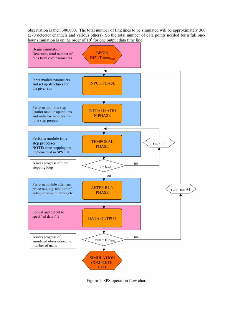
observation is then 300,000. The total number of timelines to be simulated will be approximately 300 (270 detector channels and various others). So the total number of data points needed for a full one-hour simulation is on the order of 108 for one output data time line.
run= run +1
BEGIN INPUT runstotal
INPUT PHASE
INITIALISATION PHASE
TEMPORAL PHASE
t = ttotal
no
AFTER RUN PHASE
yes
DATA OUTPUT
run = runtotal
no
SIMULATION COMPLETE:
EXIT
Begin simulation Determine total number of runs from core parameters
Input module parameters and set up structures for the given run
Perform non-time step (static) module operations and initialise modules for time step process
Perform module time step processes NOTE: time stepping not implemented in SPS 1.0
Assess progress of time stepping loop
Perform module after run processes, e.g. addition of detector noise, filtering etc.
Format and output to specified data file
Assess progress of simulated observation, i.e. number of maps
t = t +1
Figure 1: SPS operation flow chart

1.9 Module Summary
A module represents each operational process or system within the Herschel/SPIRE observing system. These are set out as follows:
No. Module Abbreviation Description 0 Core CORE Performs all operations specific to the software
simulation, i.e. operations not present in the physical system
1 Sky Simulator SKYSIM Produces a simulation of the area of sky to be observed, with a resolution finer than the SPIRE beam.
2 Input INPUT Specifies the observation in "astronomer's terms" 3 Optical System OPTICS Represents the main optical properties and parameters of
the telescope and the SPIRE photometer (including the filters), and the positional mapping of the detectors on the sky. Also produces the actual telescope boresight pointing timeline for the period of the observation, so that each detector sample can be associated with a particular point on the sky.
4 Beam Steering Mirror
BSM Produces the BSM timeline in the form of an additional pointing timeline to be superimposed on that of the telescope.
5 Observatory Function
OBSFUN Specifies the photometer observing node to be simulated in terms of the appropriate Observatory Function and its parameters, as defined in the OMD, and defines the commanded telescope pointing timeline.
6 Thermal System THERMAL Contains all information on the temperatures of the instrument and the telescope, and their temporal fluctuations.
7 Astronomical power timeline
generator
ASTROPOWER Generates a timeline for the power on each detector from the astronomical sky
8 Incident background power timeline generator
BACKGROUND Produces a timeline for the background power incident on each detector, due to all contributions from the telescope and instrument and their thermal fluctuations.
9 Bolometer voltage timeline generator
DETECTORS Produces an output voltage timeline for each detector channel at the ADC input based on the inputs from 7 and 8 and an appropriate model of the detector and its analogue electronics chain.
10 Science Data Timeline Generator
SAMPLING Produces digitised timelines for each detector channel and all housekeeping data
11 Housekeeping Data Timeline Generator
HK Produces timelines for all instrument temperatures
12 Calibrator Power Timeline Generator
PCAL Produces a timeline of the power incident on each detector from PCAL.
Table 1: Module list
1.10 Data volume
The total number of timelines to be simulated will be approximately 1200 (4 versions astronomical power, noiseless voltage, noisy voltage, filtered and sampled voltage of ~300 detector channels). Therefore the total number of data points needed for a full one-hour simulation is on the order of 3x10⁸ (as discussed in Section 1.8), based on the baseline master clock interval being 12 ms,

producing 300,000 points per timeline for a 1-hr observation. In addition to these there will also be other memory requirements from other large arrays, e.g. input sky maps.
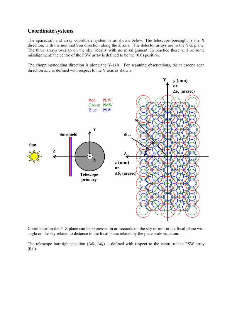
Coordinate systems
The spacecraft and array coordinate system is as shown below. The telescope boresight is the X direction, with the nominal Sun direction along the Z axis. The detector arrays are in the Y-Z plane. The three arrays overlap on the sky, ideally with no misalignment. In practice there will be some misalignment: the centre of the PSW array is defined to be the (0,0) position. The chopping/nodding direction is along the Y-axis. For scanning observations, the telescope scan direction φscan is defined with respect to the Y axis as shown. Coordinates in the Y-Z plane can be expressed in arcseconds on the sky or mm in the focal plane with angle on the sky related to distance in the focal plane related by the plate scale equation. The telescope boresight position (Δθy, Δθz) is defined with respect to the centre of the PSW array (0,0).
Y
Z
X
Sun
Sunshield
Telescope primary
y (mm) or Δθy (arcsec)
φcan
Red: PLW Green: PMW Blue: PSW
Z
z (mm) or Δθy (arcsec)
Y
Z
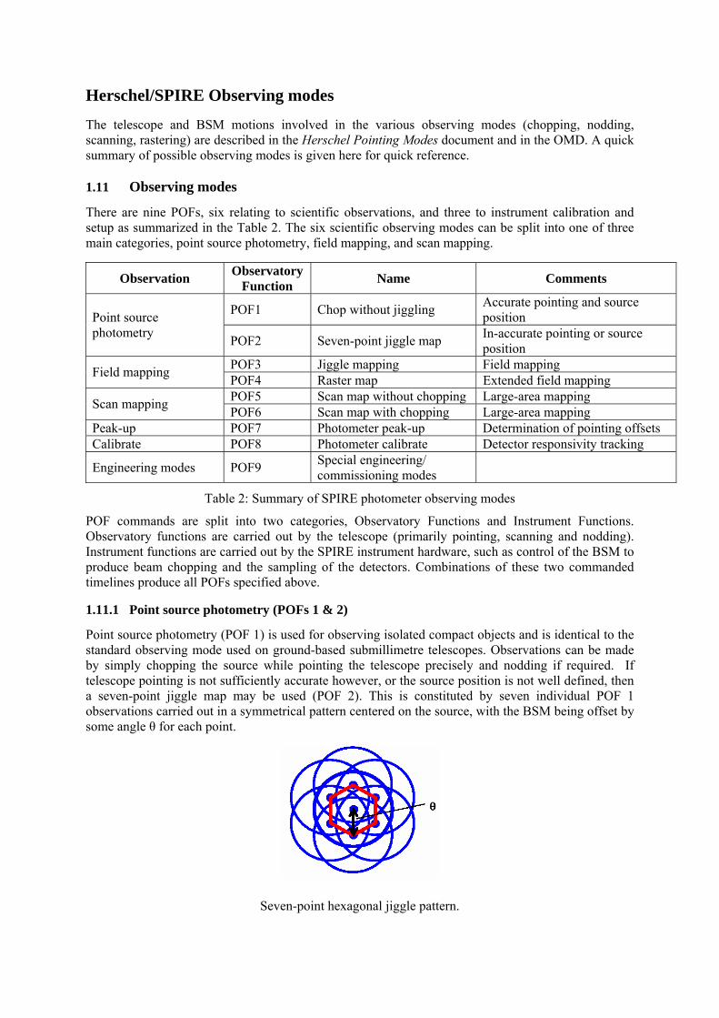
Herschel/SPIRE Observing modes
The telescope and BSM motions involved in the various observing modes (chopping, nodding, scanning, rastering) are described in the Herschel Pointing Modes document and in the OMD. A quick summary of possible observing modes is given here for quick reference. 1.11 Observing modes
There are nine POFs, six relating to scientific observations, and three to instrument calibration and setup as summarized in the Table 2. The six scientific observing modes can be split into one of three main categories, point source photometry, field mapping, and scan mapping.
Observation Observatory Function Name Comments
POF1 Chop without jiggling Accurate pointing and source position Point source
photometry POF2 Seven-point jiggle map In-accurate pointing or source position
POF3 Jiggle mapping Field mapping Field mapping POF4 Raster map Extended field mapping POF5 Scan map without chopping Large-area mapping Scan mapping POF6 Scan map with chopping Large-area mapping
Peak-up POF7 Photometer peak-up Determination of pointing offsets Calibrate POF8 Photometer calibrate Detector responsivity tracking
Engineering modes POF9 Special engineering/ commissioning modes
Table 2: Summary of SPIRE photometer observing modes
POF commands are split into two categories, Observatory Functions and Instrument Functions. Observatory functions are carried out by the telescope (primarily pointing, scanning and nodding). Instrument functions are carried out by the SPIRE instrument hardware, such as control of the BSM to produce beam chopping and the sampling of the detectors. Combinations of these two commanded timelines produce all POFs specified above.
1.11.1 Point source photometry (POFs 1 & 2)
Point source photometry (POF 1) is used for observing isolated compact objects and is identical to the standard observing mode used on ground-based submillimetre telescopes. Observations can be made by simply chopping the source while pointing the telescope precisely and nodding if required. If telescope pointing is not sufficiently accurate however, or the source position is not well defined, then a seven-point jiggle map may be used (POF 2). This is constituted by seven individual POF 1 observations carried out in a symmetrical pattern centered on the source, with the BSM being offset by some angle θ for each point.
Seven-point hexagonal jiggle pattern.
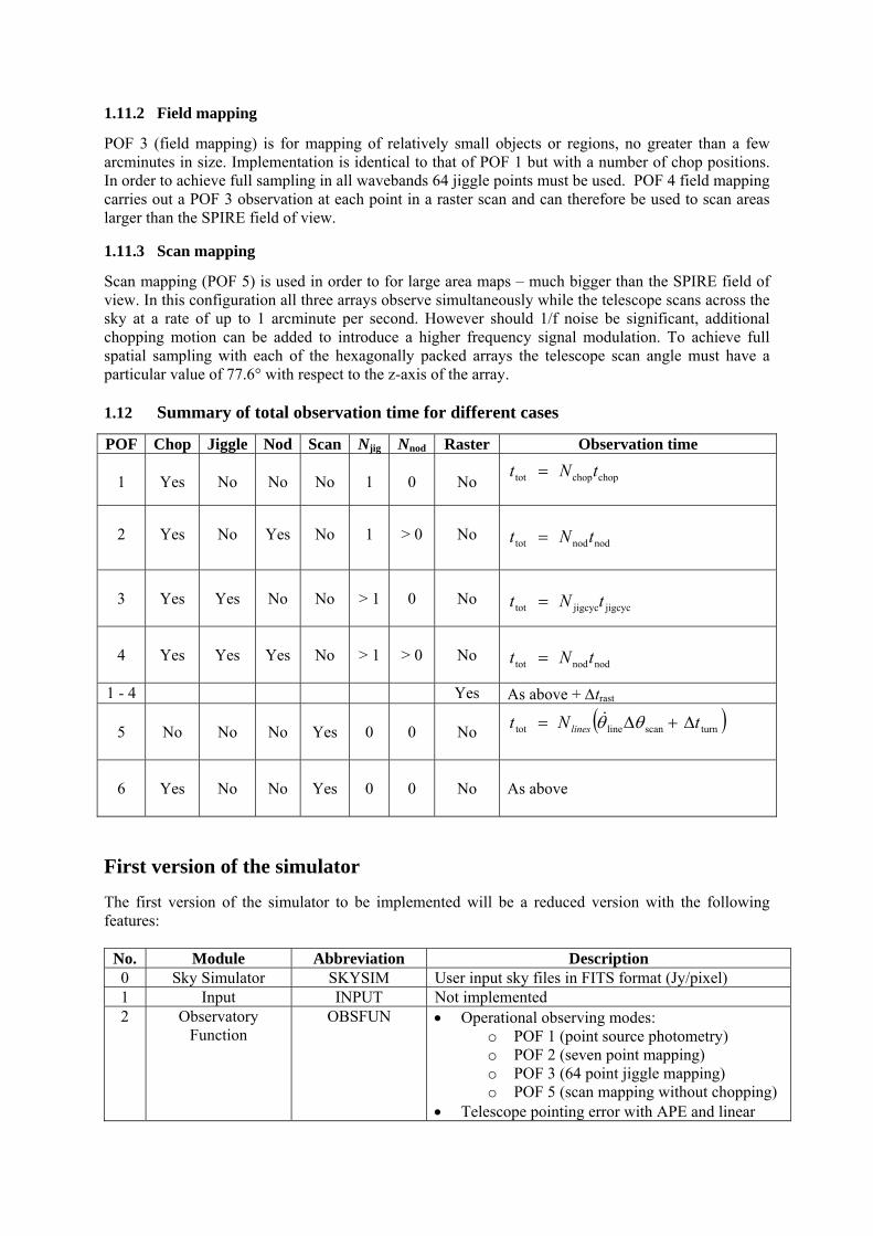
1.11.2 Field mapping
POF 3 (field mapping) is for mapping of relatively small objects or regions, no greater than a few arcminutes in size. Implementation is identical to that of POF 1 but with a number of chop positions. In order to achieve full sampling in all wavebands 64 jiggle points must be used. POF 4 field mapping carries out a POF 3 observation at each point in a raster scan and can therefore be used to scan areas larger than the SPIRE field of view.
1.11.3 Scan mapping
Scan mapping (POF 5) is used in order to for large area maps – much bigger than the SPIRE field of view. In this configuration all three arrays observe simultaneously while the telescope scans across the sky at a rate of up to 1 arcminute per second. However should 1/f noise be significant, additional chopping motion can be added to introduce a higher frequency signal modulation. To achieve full spatial sampling with each of the hexagonally packed arrays the telescope scan angle must have a particular value of 77.6° with respect to the z-axis of the array. 1.12 Summary of total observation time for different cases
POF Chop Jiggle Nod Scan Njig Nnod Raster Observation time
1
Yes
No
No
No
1
0
No
chopchoptot tNt =
2
Yes
No
Yes
No
1
> 0
No
nodnodtot tNt =
3
Yes
Yes
No
No
> 1
0
No
jigcycjigcyctot tNt =
4
Yes
Yes
Yes
No
> 1
> 0
No
nodnodtot tNt =
1 - 4 Yes As above + Δtrast
5
No
No
No
Yes
0
0
No
( )turnscanlinetot tNt lines Δ+Δ= θθ&
6
Yes
No
No
Yes
0
0
No
As above
First version of the simulator
The first version of the simulator to be implemented will be a reduced version with the following features:
No. Module Abbreviation Description 0 Sky Simulator SKYSIM User input sky files in FITS format (Jy/pixel) 1 Input INPUT Not implemented 2 Observatory
Function OBSFUN • Operational observing modes:
o POF 1 (point source photometry) o POF 2 (seven point mapping) o POF 3 (64 point jiggle mapping) o POF 5 (scan mapping without chopping)
• Telescope pointing error with APE and linear

drift implemented 3 Optical System OPTICS • Top-hat filter transmission.
• Three modelled telescope beams, one for each detector array (no hexapod), i.e. beam is assumed to be equal in all detector within a single array
• Detector selection options. • Convolution of input map with modelled beam
4 Thermal System THERMAL 1/f thermal noise variations imposed on nominal stage temperatures. Input values not well known, for testing only.
6 Beam Steering Mirror
BSM • 1, 7 and 64 point chopping operational • No noise added to commanded timeline • No power dissipation • Instantaneous BSM position switching
7 Incident background power timeline generator
BACKGROUND • Background power based on emission from all optical elements
• Optical elements assumed to be a constant temperature
• All elements assumed to emit as a blackbody 8 Astronomical
power timeline generator
ASTROPOWER Astronomical power derived from pointing at convolved input sky map (output from optics module)
9 Bolometer voltage timeline generator
DETECTORS • Output for all modules including option for non-linear operation beyond a set threshold
• Option to use measure bolometer parameters as in input
• Noise calculation performed based on calculated parameters
• Choice of white or 1/f noise addition 10 Science Data
Timeline Generator SAMPLING • Voltage data timeline filtering using measured
filter profile • Data sampling at given input frequency
11 Housekeeping Data Timeline Generator
HK Not implemented.
12 Calibrator Power Timeline Generator
PCAL Not implemented.
Simulator Set-up (Core)
The simulator operating parameters, e.g. simulator time step, output mode etc., are initialised in the same way as other modules. The core structure containing all operating parameters receives two input phases in the first of a multiple run simulation. The first phase reads in the number of runs to perform, and the second reads the remaining data. This allows for the correct output file name to be given to subsequent runs in a multi-run situation. The core routine contains no input parameters. Core parameters
Output category
Parent Module
Parameter Name Type Units Values Description / comments
User Core Operating mode op_mode Integer 0,1 0 – single opertion
1 – repeat
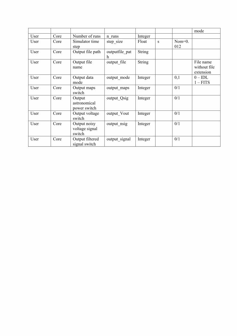
mode User Core Number of runs n_runs Integer User Core Simulator time
step step_size Float s Nom=0.
012
User Core Output file path outputfile_path
String
User Core Output file name
output_file String File name without file extension
User Core Output data mode
output_mode Integer 0,1 0 – IDL 1 – FITS
User Core Output maps switch
output_maps Integer 0/1
User Core Output astronomical power switch
output_Qsig Integer 0/1
User Core Output voltage switch
output_Vout Integer 0/1
User Core Output noisy voltage signal switch
output_nsig Integer 0/1
User Core Output filtered signal switch
output_signal Integer 0/1
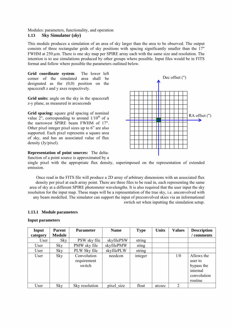
Modules: parameters, functionality, and operation 1.13 Sky Simulator (sky)
This module produces a simulation of an area of sky larger than the area to be observed. The output consists of three rectangular grids of sky positions with spacing significantly smaller than the 17" FWHM at 250 μm. There is one sky map per SPIRE array each with the same size and resolution. The intention is to use simulations produced by other groups where possible. Input files would be in FITS format and follow where possible the parameters outlined below. Grid coordinate system: The lower left corner of the simulated area shall be designated as the (0,0) position on the spacecraft z and y axes respectively. Grid units: angle on the sky in the spacecraft z-y plane, as measured in arcseconds Grid spacing: square grid spacing of nominal value 2", corresponding to around 1/10th of a the narrowest SPIRE beam FWHM of 17". Other pixel integer pixel sizes up to 6” are also supported. Each pixel represents a square area of sky, and has an associated value of flux density (Jy/pixel). Representation of point sources: The delta-function of a point source is approximated by a single pixel with the appropriate flux density, superimposed on the representation of extended emission.
Once read in the FITS file will produce a 2D array of arbitrary dimensions with an associated flux density per pixel at each array point. There are three files to be read in, each representing the same
area of sky at a different SPIRE photometer wavelengths. It is also required that the user input the sky resoluiton for the input map. These maps will be a representation of the true sky, i.e. unconvolved with
any beam modelled. The simulator can support the input of preconvolved skies via an informational swtich set when inputting the simulation setup.
1.13.1 Module parameters
Input parameters
Input category
Parent Module
Parameter Name Type Units Values Description / comments
User Sky PSW sky file skyfilePSW string User Sky PMW sky file skyfilePMW sting User Sky PLW Sky file skyfilePLW string User Sky Convolution
requirement switch
needcon integer 1/0 Allows the user to bypass the internal convolution routine
User Sky Sky resolution pixel_size float arcsec 2
RA offset (")
Dec offset (")

Output parameters
Output category
Parent Module
Parameter Name Type Units Values Description / comments
Map Sky PSW sky map skyfilePSW 2D float array
Jy / pixel
Map Sky PMW sky map skyfilePMW 2D float array
Jy / pixel
Map Sky PLW Sky map skyfilePLW 2D float array
Jy / pixel
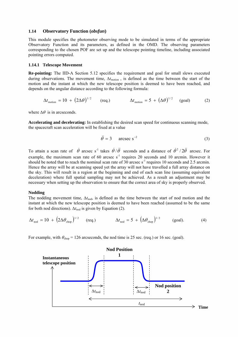
1.14 Observatory Function (obsfun)
This module specifies the photometer observing mode to be simulated in terms of the appropriate Observatory Function and its parameters, as defined in the OMD. The observing parameters corresponding to the chosen POF are set up and the telescope pointing timeline, including associated pointing errors computed. 1.14.1 Telescope Movement
Re-pointing: The IID-A Section 5.12 specifies the requirement and goal for small slews executed during observations. The movement time, Δtmotion , is defined as the time between the start of the motion and the instant at which the new telescope position is deemed to have been reached, and depends on the angular distance according to the following formula:
( ) 2/1
motion 210 θΔ+=Δt (req.) ( ) 2/1motion 5 θΔ+=Δt (goal) (2)
where Δθ is in arcseconds. Accelerating and decelerating: In establishing the desired scan speed for continuous scanning mode, the spacecraft scan acceleration will be fixed at a value 2sarcsec3 −=θ&& (3) To attain a scan rate of θ& arcsec s-1 takes θθ &&& / seconds and a distance of θθ &&& 2/2 arcsec. For example, the maximum scan rate of 60 arcsec s-1 requires 20 seconds and 10 arcmin. However it should be noted that to reach the nominal scan rate of 30 arcsec s-1 requires 10 seconds and 2.5 arcmin. Hence the array will be at scanning speed yet the array will not have travelled a full array distance on the sky. This will result in a region at the beginning and end of each scan line (assuming equivalent deceleration) where full spatial sampling may not be achieved. As a result an adjustment may be necessary when setting up the observation to ensure that the correct area of sky is properly observed. Nodding The nodding movement time, Δtnod, is defined as the time between the start of nod motion and the instant at which the new telescope position is deemed to have been reached (assumed to be the same for both nod directions). Δtnod is given by Equation (2).
( ) 2/1
chopnod 210 θΔ+=Δt (req.) ( ) 2/1chopnod 5 θΔ+=Δt (goal). (4)
For example, with θchop = 126 arcseconds, the nod time is 25 sec. (req.) or 16 sec. (goal).
Instantaneous telescope position
Time
Nod Position 1
Nod position 2 Δtnod Δtnod
tnod
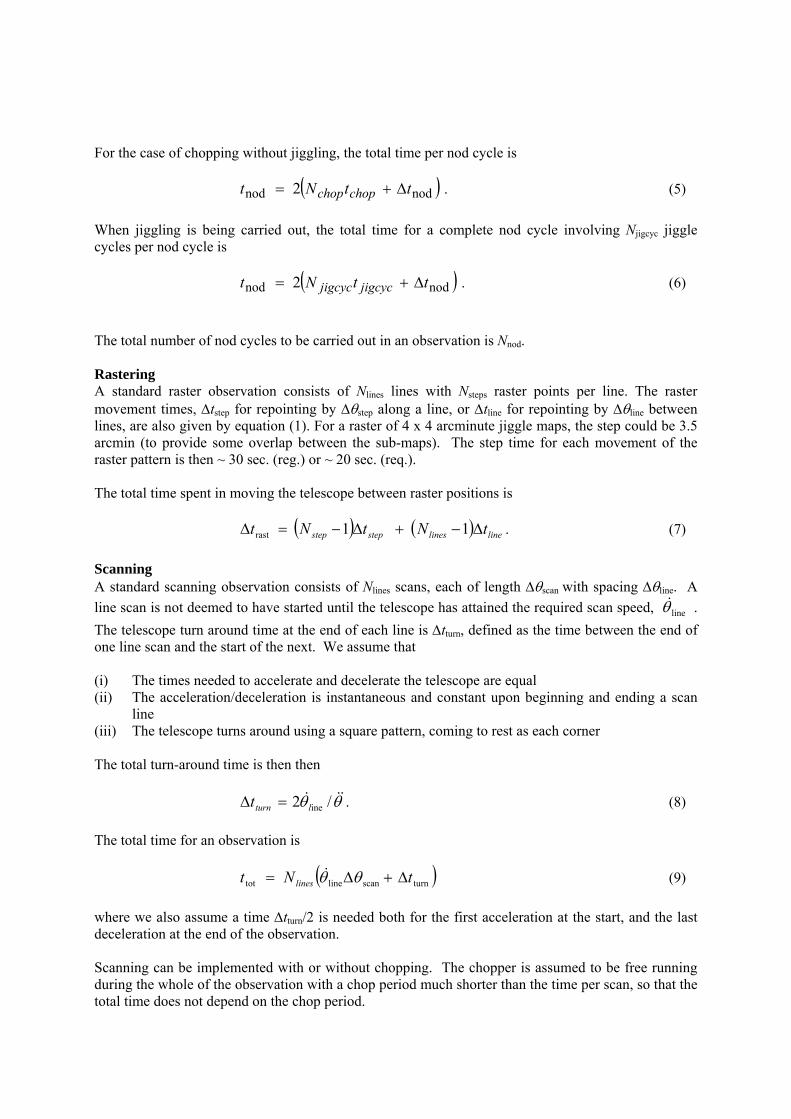
For the case of chopping without jiggling, the total time per nod cycle is ( )nodnod 2 ttNt chopchop Δ+= . (5)
When jiggling is being carried out, the total time for a complete nod cycle involving Njigcyc jiggle cycles per nod cycle is ( )nodnod 2 ttNt jigcycjigcyc Δ+= . (6)
The total number of nod cycles to be carried out in an observation is Nnod. Rastering A standard raster observation consists of Nlines lines with Nsteps raster points per line. The raster movement times, Δtstep for repointing by Δθstep along a line, or Δtline for repointing by Δθline between lines, are also given by equation (1). For a raster of 4 x 4 arcminute jiggle maps, the step could be 3.5 arcmin (to provide some overlap between the sub-maps). The step time for each movement of the raster pattern is then ~ 30 sec. (reg.) or ~ 20 sec. (req.). The total time spent in moving the telescope between raster positions is ( ) ( ) linelinesstepstep tNtNt Δ−+Δ−=Δ 11rast . (7) Scanning A standard scanning observation consists of Nlines scans, each of length Δθscan with spacing Δθline. A line scan is not deemed to have started until the telescope has attained the required scan speed, lineθ& . The telescope turn around time at the end of each line is Δtturn, defined as the time between the end of one line scan and the start of the next. We assume that (i) The times needed to accelerate and decelerate the telescope are equal (ii) The acceleration/deceleration is instantaneous and constant upon beginning and ending a scan
line (iii) The telescope turns around using a square pattern, coming to rest as each corner The total turn-around time is then then θθ &&& /2 inelturnt =Δ . (8) The total time for an observation is ( )turnscanlinetot tNt lines Δ+Δ= θθ& (9) where we also assume a time Δtturn/2 is needed both for the first acceleration at the start, and the last deceleration at the end of the observation. Scanning can be implemented with or without chopping. The chopper is assumed to be free running during the whole of the observation with a chop period much shorter than the time per scan, so that the total time does not depend on the chop period.
1.14.2 Pointing error
Pointing noise characteristics The pointing errors are defined and summarised in the IID-A Section 5.12 as follows:
Goal
qarcAPE
θ
θ&
&
03.05.1
.Re05.07.3sec][
+=
+=
Goal
qarcAME
θ
θ&
&
02.052.1
.Re03.01.3sec][
+=
+=
where θ& is in arcsec s-1.
scanningGoalscanningqingPoarcRPE
8.0.Re2.1
int03.0sec][
===
Note: RPE refers to a 1-minute period All values quoted are 68% probability (i.e., 1-σ) All information pertaining to pointing errors is subject frequent change and thus these values should only be used as a guide. Absolute pointing error The absolute pointing error (APE) is implemented as a random positional offset in both the z and y direction upon the initialisation of each new pointing (this includes the beginning of each scan line). The input is the 1 sigma RMS value based on a 2D Gaussian probability distribution function. The input value is in units of arcseconds. Relative pointing error The relative pointing error is implemented as a linear drift superimposed on the commanded telescope pointing time line. This drift occurs for the full duration of the observation. The amplitude of the drift is derived from an input drift velocity variable. This variable defines the 2D Gaussian probability distribution from which the implemented drift velocity is derived. This input as the units of arcseconds per second. The direction of drift is derived via a random number generator. This is only valid for short scans. Further work will be carried out and an improved version developed for future SPS releases. 1.14.3 Input scanning parameters
There are four important input parameters to understand when performing an extended map observation (POFs 4, 5 or 6) in order to ensure the output map covers the region required. These are centre_z, centre_y, dir_scan, scan rotation. The start parameters define the centre of the scan map pattern and are defined with reference to the input sky. The lower left corner of the input sky is regarded as the 0,0 point. These parameters have
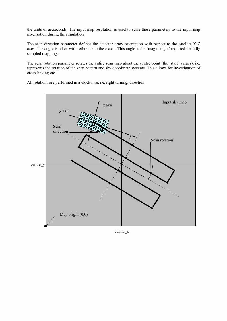
the units of arcseconds. The input map resolution is used to scale these parameters to the input map pixelisation during the simulation. The scan direction parameter defines the detector array orientation with respect to the satellite Y-Z axes. The angle is taken with reference to the z-axis. This angle is the ‘magic angle’ required for fully sampled mapping. The scan rotation parameter rotates the entire scan map about the centre point (the ‘start’ values), i.e. represents the rotation of the scan pattern and sky coordinate systems. This allows for investigation of cross-linking etc. All rotations are performed in a clockwise, i.e. right turning, direction.
Map origin (0,0)
centre_z
centre_y
Scan direction
Input sky map
Scan rotation
z axisy axis
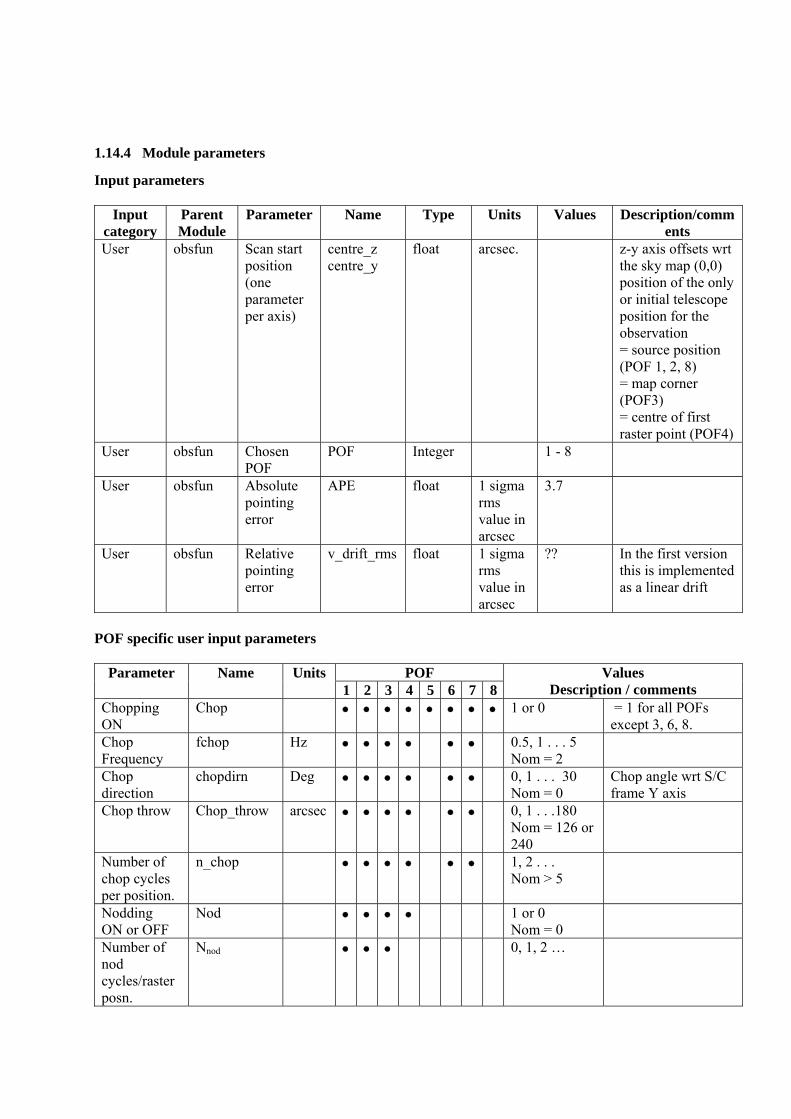
1.14.4 Module parameters
Input parameters
Input category
Parent Module
Parameter Name Type Units Values Description/comments
User obsfun Scan start position (one parameter per axis)
centre_z centre_y
float arcsec. z-y axis offsets wrt the sky map (0,0) position of the only or initial telescope position for the observation = source position (POF 1, 2, 8) = map corner (POF3) = centre of first raster point (POF4)
User obsfun Chosen POF
POF Integer 1 - 8
User obsfun Absolute pointing error
APE float 1 sigma rms value in arcsec
3.7
User obsfun Relative pointing error
v_drift_rms float 1 sigma rms value in arcsec
?? In the first version this is implemented as a linear drift
POF specific user input parameters
POF Parameter Name Units 1 2 3 4 5 6 7 8
Values Description / comments
Chopping ON
Chop • • • • • • • • 1 or 0 = 1 for all POFs except 3, 6, 8.
Chop Frequency
fchop Hz • • • • • • 0.5, 1 . . . 5 Nom = 2
Chop direction
chopdirn Deg • • • • • • 0, 1 . . . 30 Nom = 0
Chop angle wrt S/C frame Y axis
Chop throw Chop_throw arcsec • • • • • • 0, 1 . . .180 Nom = 126 or 240
Number of chop cycles per position.
n_chop • • • • • • 1, 2 . . . Nom > 5
Nodding ON or OFF
Nod • • • • 1 or 0 Nom = 0
Number of nod cycles/raster posn.
Nnod • • • 0, 1, 2 …
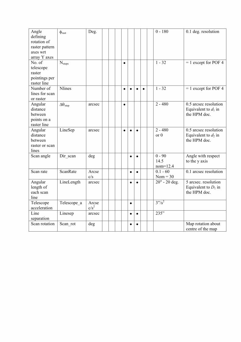
Angle defining rotation of raster pattern axes wrt array Y axes
φrast Deg. 0 - 180 0.1 deg. resolution
No. of telescope raster pointings per raster line
Nsteps • 1 - 32 = 1 except for POF 4
Number of lines for scan or raster
Nlines • • • • 1 - 32 = 1 except for POF 4
Angular distance between points on a raster line
Δθstep arcsec • 2 - 480 0.5 arcsec resolutionEquivalent to d1 in the HPM doc.
Angular distance between raster or scan lines
LineSep arcsec • • • 2 - 480 or 0
0.5 arcsec resolution Equivalent to d2 in the HPM doc.
Scan angle Dir_scan deg • • 0 - 90 14.5 nom=12.4
Angle with respect to the y axis
Scan rate ScanRate Arcsec/s
• • 0.1 - 60 Nom = 30
0.1 arcsec resolution
Angular length of each scan line
LineLength arcsec • • 20" - 20 deg. 5 arcsec. resolution Equivalent to D1 in the HPM doc.
Telescope acceleration
Telescope_a Arcsec/s2
• 3”/s2
Line separation
Linesep arcsec • • 235”
Scan rotation Scan_rot deg • • Map rotation about centre of the map

Generated command timeline: Commanded telescope position vs. time
Output category
Defining Module
Parameter Name Type Units Values Description/comments
Timeline Obsfun Telescope Pointing, z
DirZ 1D float array
arcsec True array of scanned z-coordinate positions on sky map vs. time
Timeline Obsfun Telescope Pointing, y
DirY 1D float array
arcsec True array of scanned y-coordinate positions on sky map vs. time
Timeline Obsfun Sampled telescope pointing, z
DirZsamp 1D float array
arcsec Sampled version of DirZ
Timeline Obsfun Sampled telescope pointing, y
DirYsamp 1D float array
arcsec Sampled version of DirY
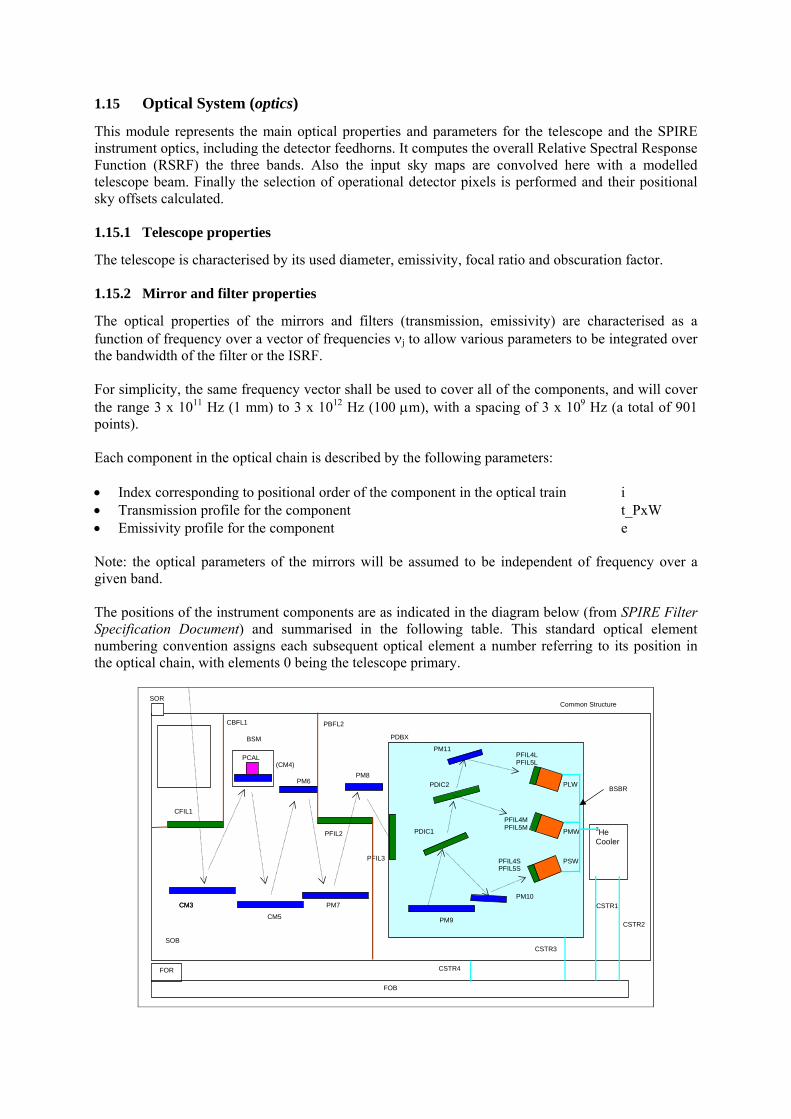
1.15 Optical System (optics)
This module represents the main optical properties and parameters for the telescope and the SPIRE instrument optics, including the detector feedhorns. It computes the overall Relative Spectral Response Function (RSRF) the three bands. Also the input sky maps are convolved here with a modelled telescope beam. Finally the selection of operational detector pixels is performed and their positional sky offsets calculated. 1.15.1 Telescope properties
The telescope is characterised by its used diameter, emissivity, focal ratio and obscuration factor. 1.15.2 Mirror and filter properties
The optical properties of the mirrors and filters (transmission, emissivity) are characterised as a function of frequency over a vector of frequencies νj to allow various parameters to be integrated over the bandwidth of the filter or the ISRF. For simplicity, the same frequency vector shall be used to cover all of the components, and will cover the range 3 x 10¹¹ Hz (1 mm) to 3 x 10¹² Hz (100 μm), with a spacing of 3 x 10⁹ Hz (a total of 901 points). Each component in the optical chain is described by the following parameters: • Index corresponding to positional order of the component in the optical train i • Transmission profile for the component t_PxW • Emissivity profile for the component e Note: the optical parameters of the mirrors will be assumed to be independent of frequency over a given band. The positions of the instrument components are as indicated in the diagram below (from SPIRE Filter Specification Document) and summarised in the following table. This standard optical element numbering convention assigns each subsequent optical element a number referring to its position in the optical chain, with elements 0 being the telescope primary.
CFIL1
PFIL3
Common Structure
CM3 CM3 CM5
PM7
( CM4) PM6 PM8
SOR
SOB
FOB
PFIL2
PCAL
FOR
PDIC1
PDIC2
PDBX
PM9
PM10
PM11
PSW
PMW
PLW
PFIL4SPFIL5S
PFIL4MPFIL5M
PFIL4LPFIL5L
3 He Cooler
CSTR1 CSTR2
CSTR3
CSTR4
BSBR
BSM CBFL1 PBFL2
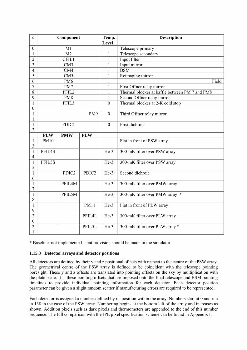
Temp. c Component Level
Description
0 M1 1 Telescope primary 1 M2 1 Telescope secondary 2 CFIL1 1 Input filter 3 CM3 1 Input mirror 4 CM4 1 BSM 5 CM5 1 Reimaging mirror 6 PM6 1 Field7 PM7 1 First Offner relay mirror 8 PFIL2 1 Thermal blocker at baffle between PM 7 and PM8 9 PM8 1 Second Offner relay mirror 10
PFIL3 0 Thermal blocker at 2-K cold stop
11
PM9 0 Third Offner relay mirror
12
PDIC1 0 First dichroic
PLW PMW PLW 13
PM10 Flat in front of PSW array
14
PFIL4S He-3 300-mK filter over PSW array
15
PFIL5S He-3 300-mK filter over PSW array
16
PDIC2 PDIC2 He-3 Second dichroic
17
PFIL4M He-3 300-mK filter over PMW array
18
PFIL5M He-3 300-mK filter over PMW array *
19
PM11 He-3 Flat in front of PLW array
20
PFIL4L He-3 300-mK filter over PLW array
21
PFIL5L He-3 300-mK filter over PLW array *
* Baseline: not implemented – but provision should be made in the simulator 1.15.3 Detector arrays and detector positions
All detectors are defined by their y and z positional offsets with respect to the centre of the PSW array. The geometrical centre of the PSW array is defined to be coincident with the telescope pointing boresight. These y and z offsets are translated into pointing offsets on the sky by multiplication with the plate scale. It is these pointing offsets that are imposed onto the final telescope and BSM pointing timelines to provide individual pointing information for each detector. Each detector position parameter can be given a slight random scatter if manufacturing errors are required to be represented. Each detector is assigned a number defined by its position within the array. Numbers start at 0 and run to 138 in the case of the PSW array. Numbering begins at the bottom left of the array and increases as shown. Addition pixels such as dark pixels and thermometers are appended to the end of this number sequence. The full comparison with the JPL pixel specification scheme can be found in Appendix I.
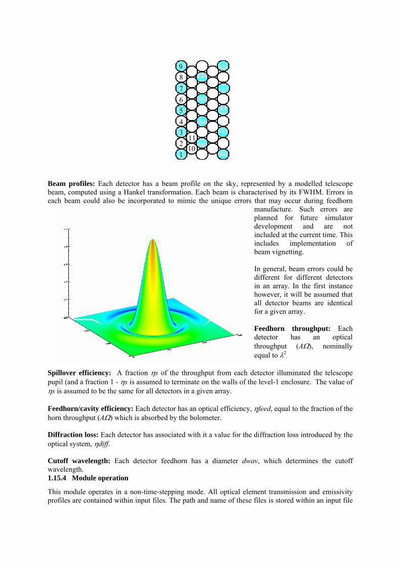
Beam profiles: Each detector has a beam profile on the sky, represented by a modelled telescope beam, computed using a Hankel transformation. Each beam is characterised by its FWHM. Errors in each beam could also be incorporated to mimic the unique errors that may occur during feedhorn
manufacture. Such errors are planned for future simulator development and are not included at the current time. This includes implementation of beam vignetting. In general, beam errors could be different for different detectors in an array. In the first instance however, it will be assumed that all detector beams are identical for a given array. Feedhorn throughput: Each detector has an optical throughput (AΩ), nominally equal to λ2
.
Spillover efficiency: A fraction ηs of the throughput from each detector illuminated the telescope pupil (and a fraction 1 - ηs is assumed to terminate on the walls of the level-1 enclosure. The value of ηs is assumed to be the same for all detectors in a given array. Feedhorn/cavity efficiency: Each detector has an optical efficiency, ηfeed, equal to the fraction of the horn throughput (AΩ) which is absorbed by the bolometer. Diffraction loss: Each detector has associated with it a value for the diffraction loss introduced by the optical system, ηdiff. Cutoff wavelength: Each detector feedhorn has a diameter dwav, which determines the cutoff wavelength. 1.15.4 Module operation
This module operates in a non-time-stepping mode. All optical element transmission and emissivity profiles are contained within input files. The path and name of these files is stored within an input file
1 2 3 4 5
1
6 7 8 9
10 11
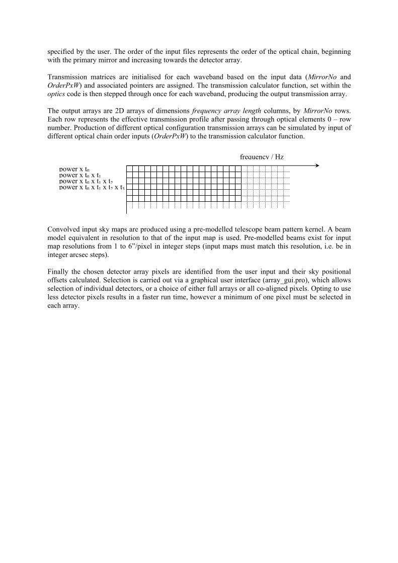
specified by the user. The order of the input files represents the order of the optical chain, beginning with the primary mirror and increasing towards the detector array. Transmission matrices are initialised for each waveband based on the input data (MirrorNo and OrderPxW) and associated pointers are assigned. The transmission calculator function, set within the optics code is then stepped through once for each waveband, producing the output transmission array.
The output arrays are 2D arrays of dimensions frequency array length columns, by MirrorNo rows. Each row represents the effective transmission profile after passing through optical elements 0 – row number. Production of different optical configuration transmission arrays can be simulated by input of different optical chain order inputs (OrderPxW) to the transmission calculator function. Convolved input sky maps are produced using a pre-modelled telescope beam pattern kernel. A beam model equivalent in resolution to that of the input map is used. Pre-modelled beams exist for input map resolutions from 1 to 6”/pixel in integer steps (input maps must match this resolution, i.e. be in integer arcsec steps). Finally the chosen detector array pixels are identified from the user input and their sky positional offsets calculated. Selection is carried out via a graphical user interface (array_gui.pro), which allows selection of individual detectors, or a choice of either full arrays or all co-aligned pixels. Opting to use less detector pixels results in a faster run time, however a minimum of one pixel must be selected in each array.
frequency / Hz power x t0 power x t0 x t1 power x t0 x t1 x t2 power x t0 x t1 x t2 x t3

1.15.5 Module parameters
Input Parameters Input category
Parent Module
Parameter Name Type Units Values Description/comments
User Optics Telescope obscuration factor
eta_obsc Float 0.872
User Optics Telescope focal ratio
Ftel Float 8.68
User Optics Array focal ratio
Ffin Float 5.0
User Optics Filter data file
filterdatafile string File containing file names + paths of files containing filter transmission profiles. List follows optical element numbering convention order.
User Optics Filter temperature file
filtertempfile string File containing optical element temperatures. List follows optical element numbering convention order. Implemented in v1.0, i.e. no temperature fluctuation with time.
User Optics Emissivity data file
emissivitydata string File containing file names + paths of files containing filter emissivity profiles. List follows optical element numbering convention order.
User Optics Gaussian FWHM Float arcsec 17, 25, Nominally

beam profile 36 assumed to be the same for all detectors
User Optics Feedhorn / cavity efficiencies
eta_feed Float 0.7 Nominally identical for all detectors in an array (maybe include some spread)
User Optics Feedhorn throughputs for each detector in the three arrays
eta_tel Float 0.7 Nominally identical for all detectors in an array
User Optics Observing wavelength
PSWlambda PMWlambda PLWlambda
Float microns 250, 363, 517
User Optics Operating detectors
detectorPSW detectorPSW detectorPSW
1D float array
Array detuning which number detector operates during an observation
User Optics Telescope effective diameter
Dtel Float m2 3.285
User Optics Optical chain order x3, one for each band
OrderPSW OrderPMW OrderPLW
1D integer
array
Optical chain order for specified waveband, e.g. for PLW, (1, 2, 3, 4, 5, 6, 7, 8, 9, 10, 11, 12, 16, 19, 20, 21).
User Optics Telescope emissivity vs. frequency
e 1x900 flaoting point array
TBD formula
Derived from input data file
User Optics Index for positional order of each component
i Integer 1 - 23
User Optics Transmission profile for each component
t 1x900 flaoting point array
Derived from input data file
User Optics Emissivity profile for each component
e 1x900 flaoting point array
Derived from input data file

User Optics Number of mirrors
MirrorNo integer 22 Number of mirrors in optical entire system (telescope + instrument)
User Optics Detector positions
PSWz_pos PSWy_pos PMWz_pos PMWy_pos PLWz_pos PLWy_pos
1D float array
arcsec Arrays defining detector positions on the sky wrt the PSW central pixel
System Sky Input sky map
SkymapPSW SkymapPMW SkymapPLW
2d float array
Jy/pixel2
System Sky Convolution requirement switch
needcon integer 1/0 Allows the user to bypass the internal convolution routine
Derived parameters
Output category
Parent Module
Parameter Name Type Units Values Description/comm
ents Map Optics Convolved
sky maps ConskyPSW ConskyPMW ConskyPLW
2D float array
Jy Maps at each wavelength of the input astronomical sky convolved with the appropriate telescope beam
System Optics Instrument spectral response function. In-band transmission from each optical element to each detector array
t_PSW t_PMW
t_PLW
2D float array
t1 x t2 x … x tn where tx is the xth optical element transmission profile
Overall spectral response of the complete system (telescope + instrument) to the detector +

System Optics Detector pixel sky offsets
PSWz_pos PSWy_pos PMWz_pos PMWy_pos PLWz_pos PLWy_pos
1D float array
arcsec Pointing offsets for operational detector array pixels.
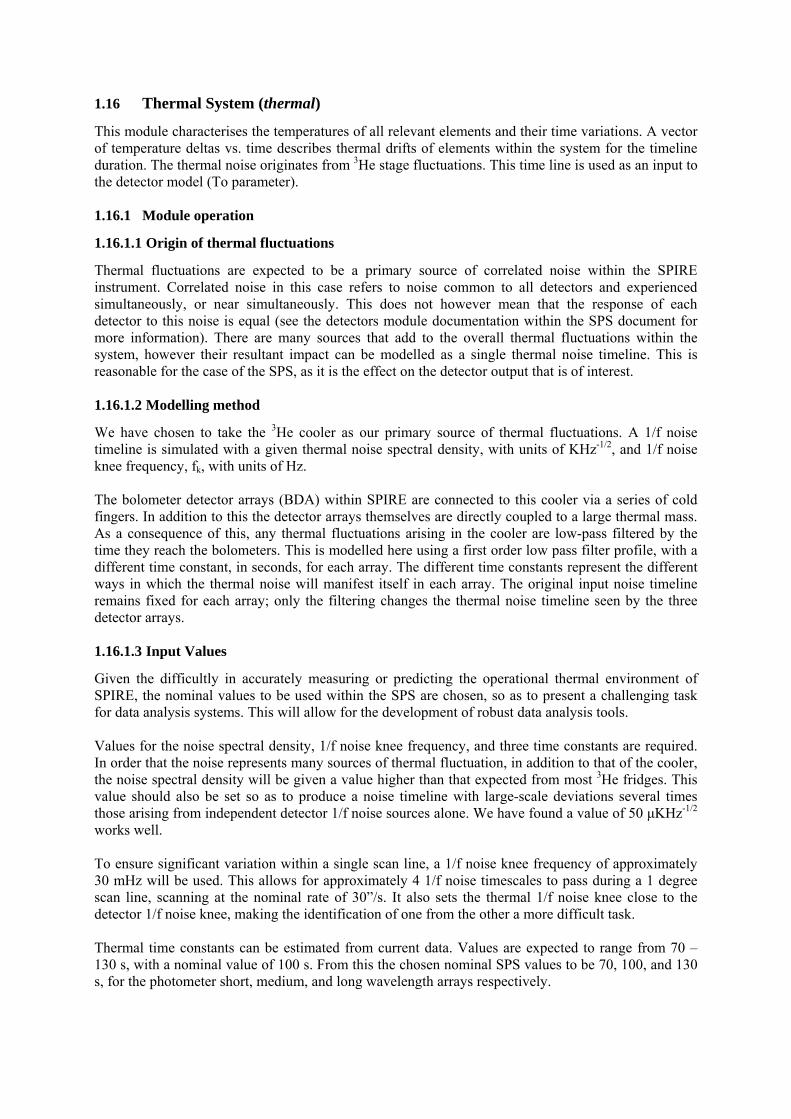
1.16 Thermal System (thermal)
This module characterises the temperatures of all relevant elements and their time variations. A vector of temperature deltas vs. time describes thermal drifts of elements within the system for the timeline duration. The thermal noise originates from 3He stage fluctuations. This time line is used as an input to the detector model (To parameter). 1.16.1 Module operation
1.16.1.1 Origin of thermal fluctuations
Thermal fluctuations are expected to be a primary source of correlated noise within the SPIRE instrument. Correlated noise in this case refers to noise common to all detectors and experienced simultaneously, or near simultaneously. This does not however mean that the response of each detector to this noise is equal (see the detectors module documentation within the SPS document for more information). There are many sources that add to the overall thermal fluctuations within the system, however their resultant impact can be modelled as a single thermal noise timeline. This is reasonable for the case of the SPS, as it is the effect on the detector output that is of interest. 1.16.1.2 Modelling method
We have chosen to take the 3He cooler as our primary source of thermal fluctuations. A 1/f noise timeline is simulated with a given thermal noise spectral density, with units of KHz-1/2, and 1/f noise knee frequency, fk, with units of Hz. The bolometer detector arrays (BDA) within SPIRE are connected to this cooler via a series of cold fingers. In addition to this the detector arrays themselves are directly coupled to a large thermal mass. As a consequence of this, any thermal fluctuations arising in the cooler are low-pass filtered by the time they reach the bolometers. This is modelled here using a first order low pass filter profile, with a different time constant, in seconds, for each array. The different time constants represent the different ways in which the thermal noise will manifest itself in each array. The original input noise timeline remains fixed for each array; only the filtering changes the thermal noise timeline seen by the three detector arrays. 1.16.1.3 Input Values
Given the difficultly in accurately measuring or predicting the operational thermal environment of SPIRE, the nominal values to be used within the SPS are chosen, so as to present a challenging task for data analysis systems. This will allow for the development of robust data analysis tools. Values for the noise spectral density, 1/f noise knee frequency, and three time constants are required. In order that the noise represents many sources of thermal fluctuation, in addition to that of the cooler, the noise spectral density will be given a value higher than that expected from most 3He fridges. This value should also be set so as to produce a noise timeline with large-scale deviations several times those arising from independent detector 1/f noise sources alone. We have found a value of 50 μKHz-1/2 works well. To ensure significant variation within a single scan line, a 1/f noise knee frequency of approximately 30 mHz will be used. This allows for approximately 4 1/f noise timescales to pass during a 1 degree scan line, scanning at the nominal rate of 30”/s. It also sets the thermal 1/f noise knee close to the detector 1/f noise knee, making the identification of one from the other a more difficult task. Thermal time constants can be estimated from current data. Values are expected to range from 70 – 130 s, with a nominal value of 100 s. From this the chosen nominal SPS values to be 70, 100, and 130 s, for the photometer short, medium, and long wavelength arrays respectively.
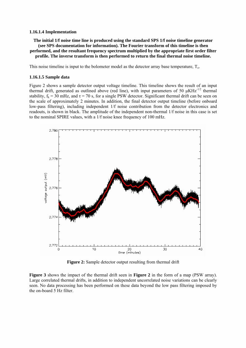
1.16.1.4 Implementation
The initial 1/f noise time line is produced using the standard SPS 1/f noise timeline generator (see SPS documentation for information). The Fourier transform of this timeline is then
performed, and the resultant frequency spectrum multiplied by the appropriate first order filter profile. The inverse transform is then performed to return the final thermal noise timeline.
This noise timeline is input to the bolometer model as the detector array base temperature, To. 1.16.1.5 Sample data
Figure 2 shows a sample detector output voltage timeline. This timeline shows the result of an input thermal drift, generated as outlined above (red line), with input parameters of 50 μKHz-1/2 thermal stability, fk = 30 mHz, and τ = 70 s, for a single PSW detector. Significant thermal drift can be seen on the scale of approximately 2 minutes. In addition, the final detector output timeline (before onboard low-pass filtering), including independent 1/f noise contribution from the detector electronics and readouts, is shown in black. The amplitude of the independent non-thermal 1/f noise in this case is set to the nominal SPIRE values, with a 1/f noise knee frequency of 100 mHz.
Figure 2: Sample detector output resulting from thermal drift
Figure 3 shows the impact of the thermal drift seen in Figure 2 in the form of a map (PSW array). Large correlated thermal drifts, in addition to independent uncorrelated noise variations can be clearly seen. No data processing has been performed on these data beyond the low pass filtering imposed by the on-board 5 Hz filter.
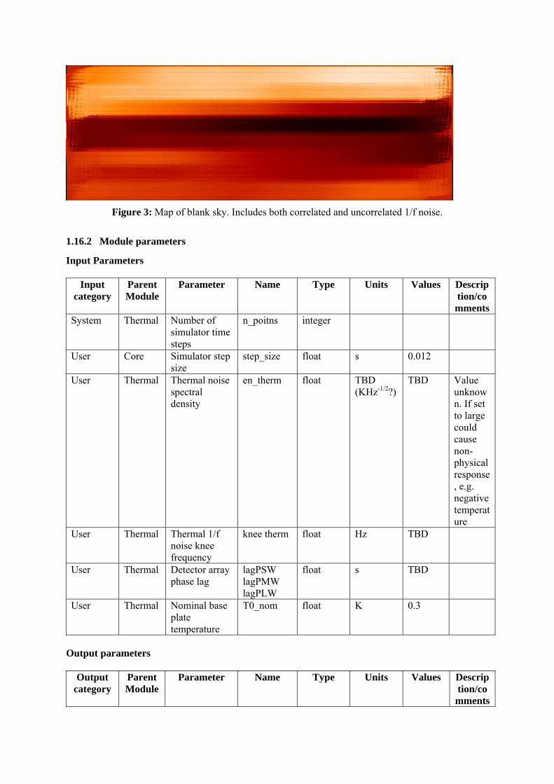
Figure 3: Map of blank sky. Includes both correlated and uncorrelated 1/f noise.
1.16.2 Module parameters
Input Parameters
Input category
Parent Module
Parameter Name Type Units Values Description/comments
System Thermal Number of simulator time steps
n_poitns integer
User Core Simulator step size
step_size float s 0.012
User Thermal Thermal noise spectral density
en_therm float TBD (KHz-1/2?)
TBD Value unknown. If set to large could cause non-physical response, e.g. negative temperature
User Thermal Thermal 1/f noise knee frequency
knee therm float Hz TBD
User Thermal Detector array phase lag
lagPSW lagPMW lagPLW
float s TBD
User Thermal Nominal base plate temperature
T0_nom float K 0.3
Output parameters
Output category
Parent Module
Parameter Name Type Units Values Description/comments

Time line Thermal Thermal noise time line
T0_PSW T0_PMW T0_PLW
1D float array
K Early model only. May introduce cooler recycle variations. Primary source of common mode noise
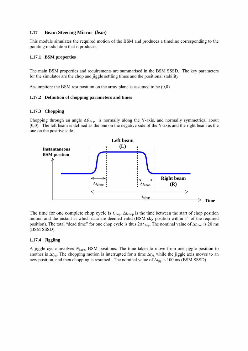
1.17 Beam Steering Mirror (bsm)
This module simulates the required motion of the BSM and produces a timeline corresponding to the pointing modulation that it produces. 1.17.1 BSM properties
The main BSM properties and requirements are summarised in the BSM SSSD. The key parameters for the simulator are the chop and jiggle settling times and the positional stability. Assumption: the BSM rest position on the array plane is assumed to be (0,0) 1.17.2 Definition of chopping parameters and times
1.17.3 Chopping
Chopping through an angle Δθchop is normally along the Y-axis, and normally symmetrical about (0,0). The left beam is defined as the one on the negative side of the Y-axis and the right beam as the one on the positive side.
The time for one complete chop cycle is tchop. Δtchop is the time between the start of chop position motion and the instant at which data are deemed valid (BSM sky position within 1” of the required position). The total “dead time” for one chop cycle is thus 2Δtchop. The nominal value of Δtchop is 20 ms (BSM SSSD). 1.17.4 Jiggling
A jiggle cycle involves Njigpos BSM positions. The time taken to move from one jiggle position to another is Δtjig. The chopping motion is interrupted for a time Δtjig while the jiggle axis moves to an new position, and then chopping is resumed. The nominal value of Δtjig is 100 ms (BSM SSSD).
Instantaneous BSM position
Time
Left beam (L)
Right beam (R) Δtchop Δtchop
tchop
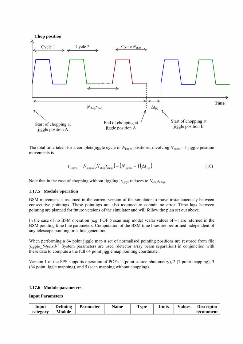
The total time taken for a complete jiggle cycle of Njigpos positions, involving Njigpos - 1 jiggle position movements is
( ) ( )( )jigjigposchopchopjigposjigcyc 1 tNtNNt Δ−+= (10)
Note that in the case of chopping without jiggling, tjigcyc reduces to Nchoptchop. 1.17.5 Module operation
BSM movement is assumed in the current version of the simulator to move instantaneously between consecutive pointings. These pointings are also assumed to contain no error. Time lags between pointing are planned for future versions of the simulator and will follow the plan set out above. In the case of no BSM operation (e.g. POF 5 scan map mode) scalar values of –1 are returned in the BSM pointing time line parameters. Computation of the BSM time lines are performed independent of any telescope pointing time line generation. When performing a 64 point jiggle map a set of normalised pointing positions are restored from file 'jiggle_64pt.xdr'. System parameters are used (detector array beam separation) in conjunction with these data to compute a the full 64 point jiggle map pointing coordinate. Version 1 of the SPS supports operation of POFs 1 (point source photometry), 2 (7 point mapping), 3 (64 point jiggle mapping), and 5 (scan mapping without chopping). 1.17.6 Module parameters
Input Parameters
Input category
Defining Module
Parameter Name Type Units Values Description/comment
Start of chopping at jiggle position A
End of chopping at jiggle position A
Start of chopping at jiggle position B
Cycle 1 Cycle 2 Cycle Nchop
Δtjig Nchoptchop Time
Chop position

s User Obsfun Photometer
observing function in operation
POF Float 1-8
User Obsfun POF 2 jiggle point separation
theta Float arcsec
User Core Simulator time step
step_size Float s 0.012
System Sky Input sky map resolution
pixel_size Float arcsec Nom=2”
System Core Simulation run number
master Integer
User Obsfun Number of chop cycles per position
n_chop Integer
User Obsfun Chop frequency
fchop Float Hz 1.98 recommended, Nom=2
System BSM Detector pixel on sky separation
pixel_separation
Float arcsec Defined for PLW array
User Obsfun Chop throw chopthrow Float arcsec User Obsfun Chop
direction chopdirn Float degrees
User Sampling Sampling time step
sampstep Float s 0.036
Output parameters
Output category
Defining Module
Parameter Name Type Units Values Description/comment
s Time line BSM Commanded
BSM position timeline, z
bsm_zcom 1D float array
arcsec Not active in SPS V1
Time line BSM Commanded BSM position timeline, y
bsm_ycom 1D flaot array
arcsec Not active in SPS V1
Time line BSM BSM position timeline, z
bsm_z 1D float array
arcsec -1 returned when POF=5
Time line BSM BSM position timeline, y
bsm_y 1D float array
arcsec -1 returned when POF=5
Time line BSM BSM chop flag
bsm_flag 1D float array
1/0
Time line BSM Sampled BSM chop
bsm_flag_samp
1D float array
1/0
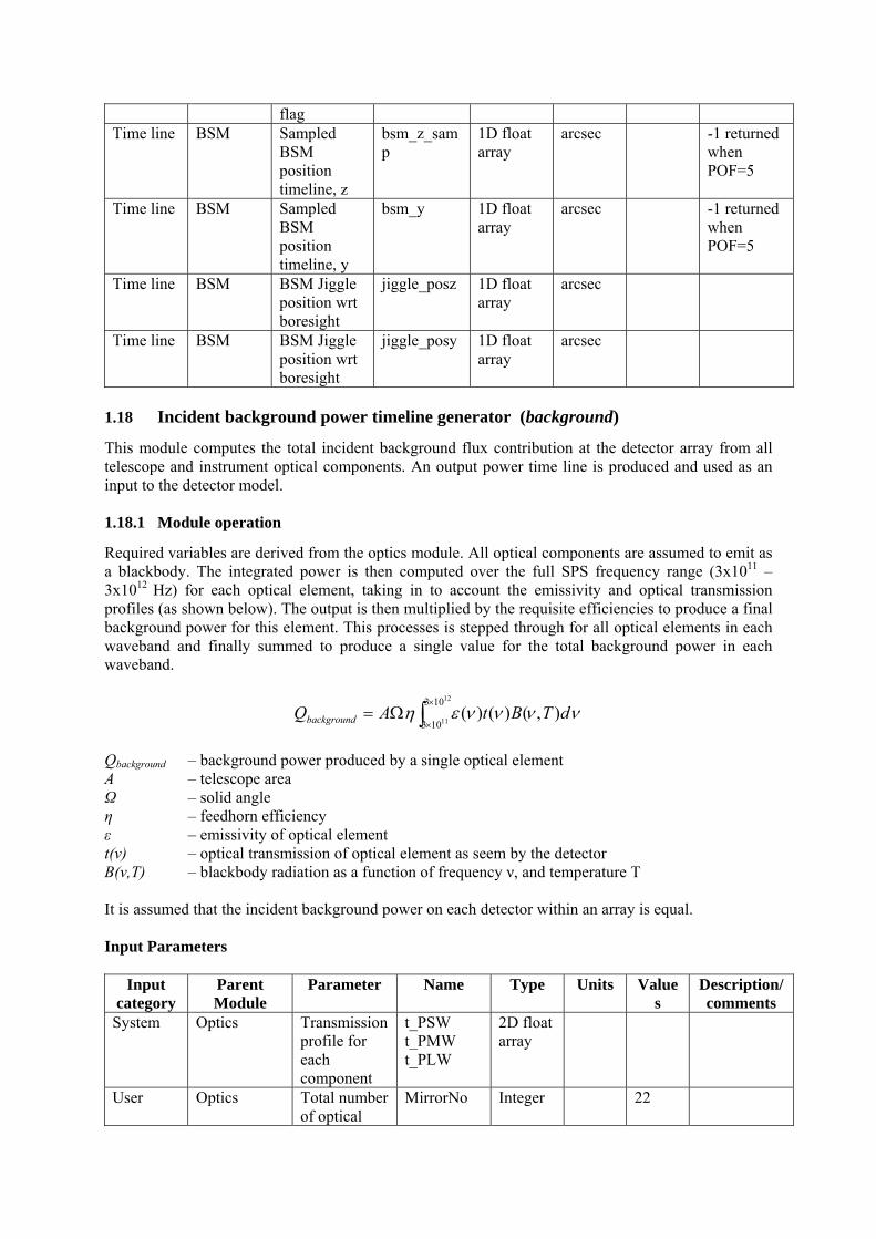
flag Time line BSM Sampled
BSM position timeline, z
bsm_z_samp
1D float array
arcsec -1 returned when POF=5
Time line BSM Sampled BSM position timeline, y
bsm_y 1D float array
arcsec -1 returned when POF=5
Time line BSM BSM Jiggle position wrt boresight
jiggle_posz 1D float array
arcsec
Time line BSM BSM Jiggle position wrt boresight
jiggle_posy 1D float array
arcsec
1.18 Incident background power timeline generator (background)
This module computes the total incident background flux contribution at the detector array from all telescope and instrument optical components. An output power time line is produced and used as an input to the detector model. 1.18.1 Module operation
Required variables are derived from the optics module. All optical components are assumed to emit as a blackbody. The integrated power is then computed over the full SPS frequency range (3x10¹¹ – 3x10¹² Hz) for each optical element, taking in to account the emissivity and optical transmission profiles (as shown below). The output is then multiplied by the requisite efficiencies to produce a final background power for this element. This processes is stepped through for all optical elements in each waveband and finally summed to produce a single value for the total background power in each waveband.
ννννεη dTBtAQbackground ),()()(12
11
103
103∫×
×Ω=
Qbackground – background power produced by a single optical element A – telescope area Ω – solid angle η – feedhorn efficiency ε – emissivity of optical element t(ν) – optical transmission of optical element as seem by the detector B(ν,T) – blackbody radiation as a function of frequency ν, and temperature T It is assumed that the incident background power on each detector within an array is equal. Input Parameters
Input category
Parent Module
Parameter Name Type Units Values
Description/comments
System Optics Transmission profile for each component
t_PSW t_PMW t_PLW
2D float array
User Optics Total number of optical
MirrorNo Integer 22
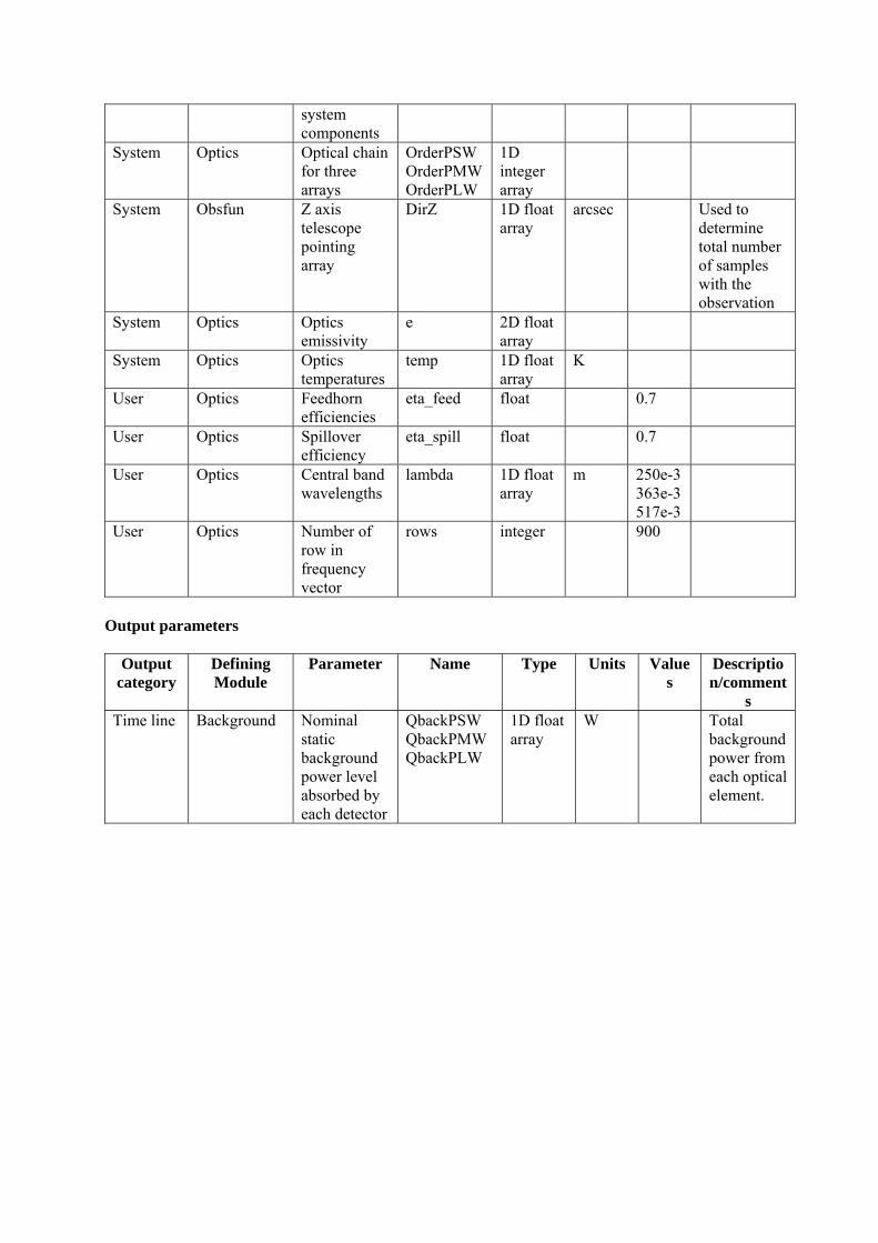
system components
System Optics Optical chain for three arrays
OrderPSW OrderPMW OrderPLW
1D integer array
System Obsfun Z axis telescope pointing array
DirZ 1D float array
arcsec Used to determine total number of samples with the observation
System Optics Optics emissivity
e 2D float array
System Optics Optics temperatures
temp 1D float array
K
User Optics Feedhorn efficiencies
eta_feed float 0.7
User Optics Spillover efficiency
eta_spill float 0.7
User Optics Central band wavelengths
lambda 1D float array
m 250e-3 363e-3 517e-3
User Optics Number of row in frequency vector
rows integer 900
Output parameters
Output category
Defining Module
Parameter Name Type Units Values
Description/comment
s Time line Background Nominal
static background power level absorbed by each detector
QbackPSW QbackPMW QbackPLW
1D float array
W Total background power from each optical element.
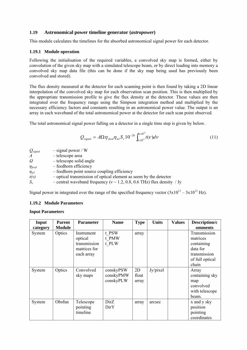
1.19 Astronomical power timeline generator (astropower)
This module calculates the timelines for the absorbed astronomical signal power for each detector. 1.19.1 Module operation
Following the initialisation of the required variables, a convolved sky map is formed, either by convolution of the given sky map with a simulated telescope beam, or by direct loading into memory a convolved sky map data file (this can be done if the sky map being used has previously been convolved and stored). The flux density measured at the detector for each scanning point is then found by taking a 2D linear interpolation of the convolved sky map for each observation scan position. This is then multiplied by the appropriate transmission profile to give the flux density at the detector. These values are then integrated over the frequency range using the Simpson integration method and multiplied by the necessary efficiency factors and constants resulting in an astronomical power value. The output is an array in each waveband of the total astronomical power at the detector for each scan point observed. The total astronomical signal power falling on a detector in a single time step is given by below.
ννηη ν dtSAQ telfeedsignal ∫×
×
−Ω=12
11
103
103
26 )(10 (11)
Qsignal – signal power / W A – telescope area Ω – telescope solid angle ηfeed – feedhorn efficiency ηtel – feedhorn point source coupling efficiency t(ν) – optical transmission of optical element as seem by the detector Sν – central waveband frequency (ν ~ 1.2, 0.8, 0.6 THz) flux density / Jy Signal power in integrated over the range of the specified frequency vector (3x10¹¹ – 3x10¹² Hz). 1.19.2 Module Parameters
Input Parameters
Input category
Parent Module
Parameter Name Type Units Values Description/comments
System Optics Instrument optical transmission matrices for each array
t_PSW t_PMW t_PLW
array Transmission matrices containing data for transmission of full optical chain
System Optics Convolved sky maps
conskyPSW conskyPMW conskyPLW
2D float array
Jy/pixel Array containing sky map convolved with telescope beam.
System Obsfun Telescope pointing timeline
DirZ DirY
array arcsec x and y sky position pointing coordinates

System Optics Detector pixel sky offsets
PSWz_pos PSWy_pos PMWz_pos PMWy_pos PLWz_pos PLWy_pos
1D float array
arcsec Pointing offsets for operational detector array pixels.
System BSM BSM pointing timeline
bsm_z bsm_y
1D float array
arcsec
User Optics Feedhorn efficiencies
eta_feed float 0.7
User Optics Aperture efficiency
eta_A float 0.7
User Obscuration factor
eta_obsc float 0.872
User Telescope effective diameter
Dtel float m 3.285
System Core Simulation run number
master Integer
User Sky Pixel size float arcsec Nom=2” Output Parameters
Output category
Parent Module
Parameter Name Type Units Values Description/comments
Time line Astro-power
Absorbed astronomical power timeline for each detector
QPSW QPMW QPLW
2D float array
W Astronomical power at each pointing position.
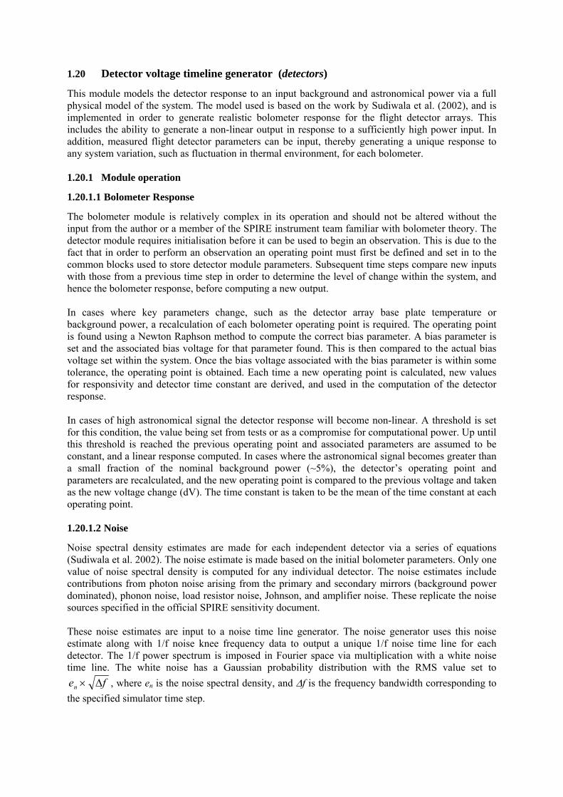
1.20 Detector voltage timeline generator (detectors)
This module models the detector response to an input background and astronomical power via a full physical model of the system. The model used is based on the work by Sudiwala et al. (2002), and is implemented in order to generate realistic bolometer response for the flight detector arrays. This includes the ability to generate a non-linear output in response to a sufficiently high power input. In addition, measured flight detector parameters can be input, thereby generating a unique response to any system variation, such as fluctuation in thermal environment, for each bolometer. 1.20.1 Module operation
1.20.1.1 Bolometer Response
The bolometer module is relatively complex in its operation and should not be altered without the input from the author or a member of the SPIRE instrument team familiar with bolometer theory. The detector module requires initialisation before it can be used to begin an observation. This is due to the fact that in order to perform an observation an operating point must first be defined and set in to the common blocks used to store detector module parameters. Subsequent time steps compare new inputs with those from a previous time step in order to determine the level of change within the system, and hence the bolometer response, before computing a new output. In cases where key parameters change, such as the detector array base plate temperature or background power, a recalculation of each bolometer operating point is required. The operating point is found using a Newton Raphson method to compute the correct bias parameter. A bias parameter is set and the associated bias voltage for that parameter found. This is then compared to the actual bias voltage set within the system. Once the bias voltage associated with the bias parameter is within some tolerance, the operating point is obtained. Each time a new operating point is calculated, new values for responsivity and detector time constant are derived, and used in the computation of the detector response. In cases of high astronomical signal the detector response will become non-linear. A threshold is set for this condition, the value being set from tests or as a compromise for computational power. Up until this threshold is reached the previous operating point and associated parameters are assumed to be constant, and a linear response computed. In cases where the astronomical signal becomes greater than a small fraction of the nominal background power (~5%), the detector’s operating point and parameters are recalculated, and the new operating point is compared to the previous voltage and taken as the new voltage change (dV). The time constant is taken to be the mean of the time constant at each operating point. 1.20.1.2 Noise
Noise spectral density estimates are made for each independent detector via a series of equations (Sudiwala et al. 2002). The noise estimate is made based on the initial bolometer parameters. Only one value of noise spectral density is computed for any individual detector. The noise estimates include contributions from photon noise arising from the primary and secondary mirrors (background power dominated), phonon noise, load resistor noise, Johnson, and amplifier noise. These replicate the noise sources specified in the official SPIRE sensitivity document. These noise estimates are input to a noise time line generator. The noise generator uses this noise estimate along with 1/f noise knee frequency data to output a unique 1/f noise time line for each detector. The 1/f power spectrum is imposed in Fourier space via multiplication with a white noise time line. The white noise has a Gaussian probability distribution with the RMS value set to
fen Δ× , where en is the noise spectral density, and Δf is the frequency bandwidth corresponding to the specified simulator time step.
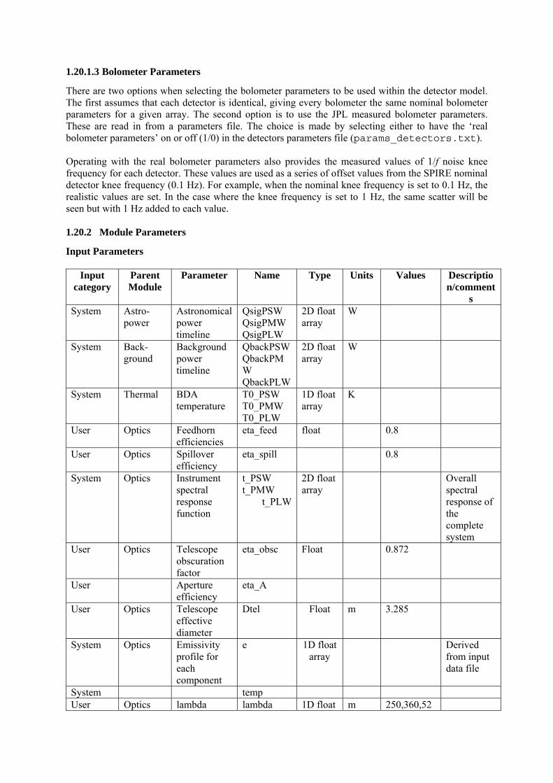
1.20.1.3 Bolometer Parameters
There are two options when selecting the bolometer parameters to be used within the detector model. The first assumes that each detector is identical, giving every bolometer the same nominal bolometer parameters for a given array. The second option is to use the JPL measured bolometer parameters. These are read in from a parameters file. The choice is made by selecting either to have the ‘real bolometer parameters’ on or off (1/0) in the detectors parameters file (params_detectors.txt). Operating with the real bolometer parameters also provides the measured values of 1/f noise knee frequency for each detector. These values are used as a series of offset values from the SPIRE nominal detector knee frequency (0.1 Hz). For example, when the nominal knee frequency is set to 0.1 Hz, the realistic values are set. In the case where the knee frequency is set to 1 Hz, the same scatter will be seen but with 1 Hz added to each value. 1.20.2 Module Parameters
Input Parameters
Input category
Parent Module
Parameter Name Type Units Values Description/comment
s System Astro-
power Astronomical power timeline
QsigPSW QsigPMW QsigPLW
2D float array
W
System Back-ground
Background power timeline
QbackPSW QbackPMW QbackPLW
2D float array
W
System Thermal BDA temperature
T0_PSW T0_PMW T0_PLW
1D float array
K
User Optics Feedhorn efficiencies
eta_feed float 0.8
User Optics Spillover efficiency
eta_spill 0.8
System Optics Instrument spectral response function
t_PSW t_PMW
t_PLW
2D float array
Overall spectral response of the complete system
User Optics Telescope obscuration factor
eta_obsc Float 0.872
User Aperture efficiency
eta_A
User Optics Telescope effective diameter
Dtel Float m 3.285
System Optics Emissivity profile for each component
e 1D float array
Derived from input data file
System temp User Optics lambda lambda 1D float m 250,360,52

array 0 um User CORE Simulator
time step length
Step_size Float s 12ms
User Use of real bolometer parameters switch
real_bolo_parameters
Integer 0/1 If set to 0 then nominal values used, else data read from file
User Nominal 1/f detector noise knee frequency
fknee_nom Integer Hz 0.1
User Detectors Implemented 1/f noise knee frequency
fknee 1D float array
Hz 1 value per detector
System Noise calculation switch
noise_init=en_det
KEYWORD
System Module initialisation switch
IN KEYWORD
User Thermal Nominal base plate temperature
T0_nom float K 0.3
User Detectors Detector noise switch
noise_10 Integer 0/1
User Detectors Detector 1/f noise switch
fnoise_10 Integer 0/1
Output parameters
Output category
Parent Module
Parameter Name Type Units Values Description/comment
s Time line Detectors Detector
voltage output (noiseless)
VoutPSW VoutPMW VoutPLW
2D float array
V Noiseless voltage time line. Save to disk to save active memory
Time line Detectors Signal + noise voltage detector output
nsigPSW nsigPMW nsigPLW
2D float array
V Noiseless voltage time line. Save to disk to save active memory
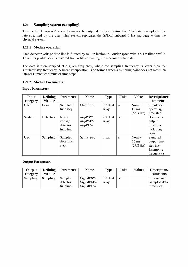
1.21 Sampling system (sampling)
This module low-pass filters and samples the output detector data time line. The data is sampled at the rate specified by the user. This system replicates the SPIRE onboard 5 Hz analogue within the physical system. 1.21.1 Module operation
Each detector voltage time line is filtered by multiplication in Fourier space with a 5 Hz filter profile. This filter profile used is restored from a file containing the measured filter data. The data is then sampled at a given frequency, where the sampling frequency is lower than the simulator step frequency. A linear interpolation is performed when a sampling point does not match an integer number of simulator time steps. 1.21.2 Module Parameters
Input Parameters
Input category
Defining Module
Parameter Name Type Units Value Description/comments
User Core Simulator time step
Step_size 2D float array
s Nom = 12 ms (83.3 Hz)
Simulator operating time step
System Detectors Noisy voltage detector time line
nsigPSW nsigPMW nsigPLW
2D float array
V Bolometer output timelines including noise
User Sampling Sampled data time step
Samp_step Float s Nom = 36 ms (27.8 Hz)
Sampled output time step (i.e. 1/samping frequency)
Output Parameters
Output category
Defining Module
Parameter Name Type Units Values Description/comments
Sampling Sampling Sampled detector timelines
SignalPSW SignalPMW SignalPLW
2D float array
V Filtered and sampled data timelines.
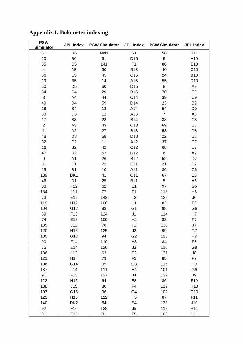
Appendix I: Bolometer indexing
PSW Simulator JPL Index PSW Simulator JPL Index PSW Simulator JPL Index
51 D6 NaN R1 58 D11 20 B6 61 D16 9 A10 35 C5 141 T1 86 E10 4 A5 30 B16 40 C10 66 E5 45 C15 24 B10 19 B5 14 A15 55 D10 50 D5 60 D15 8 A9 34 C4 29 B15 70 E9 3 A4 44 C14 39 C9 49 D4 59 D14 23 B9 18 B4 13 A14 54 D9 33 C3 12 A13 7 A8 17 B3 28 B14 38 C8 2 A3 43 C13 69 E8 1 A2 27 B13 53 D8 48 D3 58 D13 22 B8 32 C2 11 A12 37 C7 16 B2 42 C12 68 E7 47 D2 57 D12 6 A7 0 A1 26 B12 52 D7 31 C1 72 E11 21 B7 15 B1 10 A11 36 C6
139 DK1 41 C11 67 E6 46 D1 25 B11 5 A6 88 F12 62 E1 97 G5
134 J11 77 F1 113 H6 73 E12 142 T2 129 J6
119 H12 108 H1 82 F6 104 G12 93 G1 98 G6 89 F13 124 J1 114 H7 74 E13 109 H2 83 F7
135 J12 78 F2 130 J7 120 H13 125 J2 99 G7 105 G13 94 G2 115 H8 90 F14 110 H3 84 F8 75 E14 126 J3 110 G8
136 J13 63 E2 131 J8 121 H14 79 F3 85 F9 106 G14 95 G3 116 H9 137 J14 111 H4 101 G9 91 F15 127 J4 132 J9
122 H15 64 E3 86 F10 138 J15 80 F4 117 H10 107 G15 96 G4 102 G10 123 H16 112 H5 87 F11 140 DK2 64 E4 133 J10 92 F16 128 J5 118 H11 91 E15 81 F5 103 G11
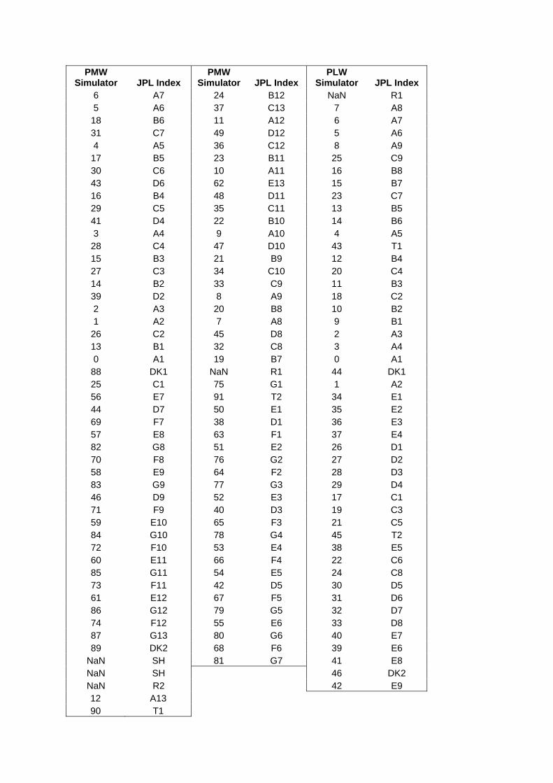
PMW Simulator JPL Index
PMW Simulator JPL Index
PLW Simulator JPL Index
6 A7 24 B12 NaN R1 5 A6 37 C13 7 A8
18 B6 11 A12 6 A7 31 C7 49 D12 5 A6 4 A5 36 C12 8 A9
17 B5 23 B11 25 C9 30 C6 10 A11 16 B8 43 D6 62 E13 15 B7 16 B4 48 D11 23 C7 29 C5 35 C11 13 B5 41 D4 22 B10 14 B6 3 A4 9 A10 4 A5
28 C4 47 D10 43 T1 15 B3 21 B9 12 B4 27 C3 34 C10 20 C4 14 B2 33 C9 11 B3 39 D2 8 A9 18 C2 2 A3 20 B8 10 B2 1 A2 7 A8 9 B1
26 C2 45 D8 2 A3 13 B1 32 C8 3 A4 0 A1 19 B7 0 A1
88 DK1 NaN R1 44 DK1 25 C1 75 G1 1 A2 56 E7 91 T2 34 E1 44 D7 50 E1 35 E2 69 F7 38 D1 36 E3 57 E8 63 F1 37 E4 82 G8 51 E2 26 D1 70 F8 76 G2 27 D2 58 E9 64 F2 28 D3 83 G9 77 G3 29 D4 46 D9 52 E3 17 C1 71 F9 40 D3 19 C3 59 E10 65 F3 21 C5 84 G10 78 G4 45 T2 72 F10 53 E4 38 E5 60 E11 66 F4 22 C6 85 G11 54 E5 24 C8 73 F11 42 D5 30 D5 61 E12 67 F5 31 D6 86 G12 79 G5 32 D7 74 F12 55 E6 33 D8 87 G13 80 G6 40 E7 89 DK2 68 F6 39 E6
NaN SH 81 G7 41 E8 NaN SH 46 DK2 NaN R2 42 E9 12 A13 90 T1


![HERSCHEL-SPIRE FOURIER TRANSFORM SPECTROMETER … · 2020. 10. 12. · HERSCHEL-SPIRE FOURIER TRANSFORM SPECTROMETER OBSERVATIONS OF EXCITED CO AND [Ci] IN THE ANTENNAE (NGC 4038/39):](https://img.pdfslide.net/doc/110x75/60de72d1a836221d6a62e755/herschel-spire-fourier-transform-spectrometer-2020-10-12-herschel-spire-fourier.jpg)