Chastaing Gaëlle

Risø Laboratory - DTU

Second Year’s Training ReportJune - August 2009

Meta-Analysis on grain yield effectsof cereals-legume intercropping

Risø-DTU Supervisors

Østergård HanneLars Pødenphant

KU-life Supervisors

Bjarne JørnsgårdIb Skovgaard

City : Roskilde Country : Denmark

1

Contents

Introduction 4

Risø National Laboratory 7

Meta analysis for Agriculture 11

1 Project introduction 121.1 Agricultural design . . . . . . . . . . . . . . . . . . . . . . . . . . . . . . . . . . . . 12

1.1.1 Principles and strategies . . . . . . . . . . . . . . . . . . . . . . . . . . . . . 121.1.2 Plot designs . . . . . . . . . . . . . . . . . . . . . . . . . . . . . . . . . . . . 13

1.2 Project framework . . . . . . . . . . . . . . . . . . . . . . . . . . . . . . . . . . . . 13

2 Preliminaries 142.1 Data collection . . . . . . . . . . . . . . . . . . . . . . . . . . . . . . . . . . . . . . 142.2 The choice of the measure effect . . . . . . . . . . . . . . . . . . . . . . . . . . . . 14

3 Data description 173.1 The data . . . . . . . . . . . . . . . . . . . . . . . . . . . . . . . . . . . . . . . . . 173.2 Descriptive Statistics . . . . . . . . . . . . . . . . . . . . . . . . . . . . . . . . . . . 17

4 Meta analysis : First approach 204.1 Modeling . . . . . . . . . . . . . . . . . . . . . . . . . . . . . . . . . . . . . . . . . 204.2 The LER effect measure . . . . . . . . . . . . . . . . . . . . . . . . . . . . . . . . . 21

4.2.1 Estimation . . . . . . . . . . . . . . . . . . . . . . . . . . . . . . . . . . . . 214.2.2 Interpretation . . . . . . . . . . . . . . . . . . . . . . . . . . . . . . . . . . . 214.2.3 Publication bias . . . . . . . . . . . . . . . . . . . . . . . . . . . . . . . . . 22

4.3 The selection and complementary effects . . . . . . . . . . . . . . . . . . . . . . . . 244.3.1 Estimation . . . . . . . . . . . . . . . . . . . . . . . . . . . . . . . . . . . . 244.3.2 Interpretation . . . . . . . . . . . . . . . . . . . . . . . . . . . . . . . . . . . 254.3.3 The "leave-one-out" analysis . . . . . . . . . . . . . . . . . . . . . . . . . . 26

5 Meta analysis : Second approach 295.1 Modeling . . . . . . . . . . . . . . . . . . . . . . . . . . . . . . . . . . . . . . . . . 295.2 Method and results . . . . . . . . . . . . . . . . . . . . . . . . . . . . . . . . . . . . 29

5.2.1 LER estimations . . . . . . . . . . . . . . . . . . . . . . . . . . . . . . . . . 305.2.2 The double effect estimations . . . . . . . . . . . . . . . . . . . . . . . . . . 30

Conclusion 32

Annexes 36

Bibliography 46

2

3

Introduction

Going abroad is a good opportunity to improve his foreign tongue practice, but it is also a richhuman experience we can hardly forget.An internship in Denmark was much better because I could not imagine I was going to learn verymany things in such a very short time : Besides an adaptation to a different culture and differentdaily habits, it was my first experience in a National Laboratory, and among biologists.

Although not clear for me and considered as a bit difficult, the subject dealt with a meta anal-ysis on cultures of intercropping of food and feed crops. The part of my job was then to contributeto show the benefit of farming practices thanks to statistics, whereas biologists I worked with hadbeen in charge to show advantages by experiments.My last internship was also about Agriculture and crop study, so I was more or less prepared tothese kind of data, and elements which can contribute to get good yields. I enjoyed this last experi-ence, that is why I wanted to do it again, but this time, in a more environmentally friendly approach.

This project was indeed about farming and biodiversity, but this time, the topic was moreabout practices, mainly the intercropping I did not know at all, and my first job was to understandperfectly this principle [1], [2]. In parallel, I had to understand the meta analysis principles thanksto tutorials [3], and anything I could find.The second step, and a new task, was to collect data by my own, my first panic ! How could I dothat ? Fortunately, people were here to help me.

After many discussions about the article selection, the measure to use and different features,we took the decision to do several analysis, because we had several perspectives and leads; it wasvery enjoyable because it meant I was free to try many different technics, and to learn a lot.

4

5

Risø National LaboratoryDTU

6

7

Their missions

Located in Roskilde, the second biggest city of the ZealandIsland, after Copenhagen, the laboratory is attached to theTechnical University of Denmark, and is focused on researchfor sustainable energy.

Composed of 7 departments, the research areas are sustain-able energy supply, climate change mitigation and nuclear tech-nologies in order to find sustainable solutions for Danish dailylife. Using natural resources like wind or sun, they also leadresearch on plant characteristics to try to understand and usethe Environment for the future.

One of these divisions is the biosystems division, which spe-ciality is to study how can be used biomass for the energy production. This section consists ofseveral divisions with specific tasks, and my project was affiliated of the biomass and bioenergyprogramme(NRG).

The NRG Programme

The experiments led in the biosystem division mainly concernedthe analysis and treatment of plant biomass, its conversion into bioen-ergy and biomaterials. From practice to theory, the main task is tofind practical idea_ and see if it is possible_ to encourage farms toreduce their CO2 production, and show them it could represent realfinancial and time-saving advantages.

At the same time, scientists study how crops can be grown in anenvironment-friendly way, their properties, and which of these prop-erties have an impact on how efficiently the plants are converted intoenergy and materials.

This programme is composed of approximately 30 people, consistedof technicians who lead experiments, researchers who, based on results of technicians’ experiments,work on theoretical issues, try to solve and bring new ideas. The team is also composed of PhDstudent, post-PhD, researcher assistants, but also temporary trainees and summer students.

Most of the programme has a biological or/and chemical background. My project was mainlysupervised my Risø supervisor, Hanne Østergård,a biometrician and a PhD student, Lars Pøden-phant, working on meta analysis. In addition, 2 supervisors from Copenhagen University, Facultyof Life Science were involved : an agronomist, Bjarne Jørnsgård, and a statistician, Ib MichaelSkovgaard.

The work strategy for me was to understand perfectly what was expected, to find some docu-mentations and papers related to the problems, and to understand by my own how to deal withthe subject. Of course, people around this project guided me to the right directions, made mesuggestions, and replied to my biological-statistical questioning.

8

9

Meta analysis for Agriculture

10

11

Chapter 1

Project introduction

1.1 Agricultural designIn order to reduce costs and increase profits, while at the same time sustaining our land resource

base, sustainable agriculture seeks to use Nature as the model for designing agricultural systems.One of these concepts is the intercropping, a simultaneous cultivation of more than one crop specieson the same piece of land, which the main feature is to promote interaction between species.

Looking for a production optimization, this practice is based on principles we have to understandwell to handle the following study.

1.1.1 Principles and strategiesWhen two or more species are growing together, each must have adequate space and architec-

ture to produce an optimum yield.

To accomplish this, spatial arrangement has to be considered firstly.There are at least three basic spatial arrangement used in intercropping, one of the most commonbeing the row intercropping, which consists in growing two or more crops at the same time withat least one crop planted in rows. Other arrangements exist, like the strip (crops are growing instrips) or mixed intercropping (no distinct row designs), and all these have to take into accountthe plant density.

Indeed, the seeding rates do not have to overload the field, unless to slow the yield down becauseof intense overcrowding.The idea is to find the optimum proportion of seed density to be used in intercropping, whichcould be difficult because a lower rate of one of the crop can produce the same yield at the endthan a higher rate of an other species. Therefore, in order to compare the monocropping with theintercropping, a seed proportion of one crop from monocropping is considered in intercropping,usually 50% of monocrop seed rate is used in a cereal-legume intercropping. Nonetheless, theseproportions can be different, according to the species used and the study’s goal.

The plot design is another important concept, used to observe the treatment effects on crops.The design choice has an impact on the analysis of variance led, and has a large importance for ameta analysis.For these reasons, I will develop the 2 two most used in agricultural design, and I will try to stressup their differences in the statistical analysis.

12

1.1.2 Plot designsIn agricultural research, experimental designs are selected according to the number of factors,

and the importance one can have compared with an other. According to the design used, analysisdiffer from degrees of freedom and dependance, drawing to different conclusions if these last arebadly used.However, the common point is that the replication (i.e. the repetition of the experiment) is con-sidered as a factor, but its effect does not matter.

We will focus on the two most used plot design : The randomized complete block design, andthe split plot design.

The randomized complete blocks design is one of the most widely used, especially suited forfield experiments when the number of treatments is not large. The main specificity of this designis the presence of equal size blocks, containing all the treatments.The process is applied separatelyand independently to each of the blocks.It is a classical case of ANOVA in analysis of variance.

The split plot design is suited for a two-factor experiment, with the feature that one of the fac-tors is assigned to the main-plot factor, whereas the other is the subplot factor. In this situation,the precision of the effects of the main-plot factor is sacrificed to improve that of the subplot fac-tor. The effect measurement of the interactions is also more precise than in a randomized completeblock design.Then, if a study wants to put more importance to a factor to one other, a split plot design isconsidered.

The understanding of these designs is very important for the information’s extraction used ina meta analysis, but also for the whole project arose now.

1.2 Project frameworkTo show the multiple benefits of intercropping, one of these strategies has been carried out

through an field experiment with specific conditions : During 3 years and in 2 different locations_in a sandy loam soil, and a sandy soil_ in Denmark, scientists have observed the effects of mixingcereals and legumes in a 2-species organic intercropping. The cereals culture was spring barley,observed with pea, faba bean and lupin respectively, in randomized complete blocks.For each of the three crop combination, for each condition, the yield and the protein content havebeen studied in pure crop and intercrop.

Because one experiment is not enough to lead a statistical analysis, it gets usual that Agron-omy has recourse to the meta analysis in order to collect more data, despite the loss of quality ofinformation due to the fact that only treated data are available.

The aim of this process is to extract data from publications treating intercropping of cerealsand legume to determine the effects of dual intercropping of either legume or cereals on yield per-formance.After this first step, an effect measure is selected to reply to the problematic : Has intercroppinggot a positive effect on grain yield and protein grain contents ?

At last, according to the variance chosen and extracted from articles, technics will be set up tolead an analysis and answer to the questions, regarding the effect measure(s) chosen.

13

Chapter 2

Preliminaries

2.1 Data collection

Database retrievalThe criteria for retrieval of studies for the meta-analysis were publication in a peer-reviewed

journal included in the DTU Article Database, from year 1900 and onwards.

Papers reporting on grain yield of sole crops and mixtures of cereals with legumes were searchedfor. The search [wheat or oat or barley or triticale or cereal ] and [legume or lupin or faba or pea]and [yield or protein or nitrogen] and [intercrop* or species mixture] provided 204 papers. Titlesand abstracts of these papers were studied by Bjarne Jørnsgård, and only papers where grain yieldof the crops were recorded were selected for further investigation and full text retrieval. It impliesthat both pure and intercrop yields for both species (focus on 2-species intercropping) had to beprovided.

From these 204 papers, only 10 has been retrieved but one study has usually more than onemixture (the several effect measures), so the dataset is reasonably large to carry out an analysis.The references are [4], [5], [6], [7], [8], [9], [10], [11], [12] & [13].

Data extractionThe database gathers information on growing conditions, such as fertilizer use, seed densities

or type of soil, but also grain yields, variance and seed proportions were collected for analysis.From this set, grain yields will be used to get an effect measure, whereas the choice of the weight(to get an estimation of the overall mean effect) will depend on provided information in publications.

The measure effect has to be easily interpretable and it has to compare the pure and theintercrop yield using both to answer to our problematic.

2.2 The choice of the measure effectFor this meta-analysis, 2 measures are suggested : The Land Equivalent Ratio (LER) and the

overall gain of intercropping proposed by Loreau and Hector [14] en 2001 .

The first one is a simple way to compare the pure yield with the intercropping yield by a sumof ratio, whereas the other is a measure based on the separation of a "selection effect" and a"complementary effect".

14

Land Equivalent RatioThe Land Equivalent Ratio (LER) is a measure introduced by Mead and Willey in 1980 to

compare the yields obtained by polyculture with yields obtained by monoculture of the same crops.

In our situation (i.e 2 species are intercropped), the expression is :

LER =YI1

y1+

YI2

y2

when

• yi is the yield of the pure crop i (i=1,2)

• YIiis the yield of the intercropped culture i (i=1,2)

A LER greater than 1 shows that intercropping is advantageous, whereas less that 1 shows adisadvantage.

However, we often notice, by application, that the LER can be above 1, and yet the purecrop of one species is better than the mixture yield, or one of the 2 species loses productivityin intercropping. In this situation, the intercropping benefit remains unknown, because a morecomplex procedure occurs.

To remedy to this problem, Loreau and Hector [14] introduced an other measure, the covari-ance function firstly defined for the yield, but also used to measure other kinds of production (e.g.biomass).

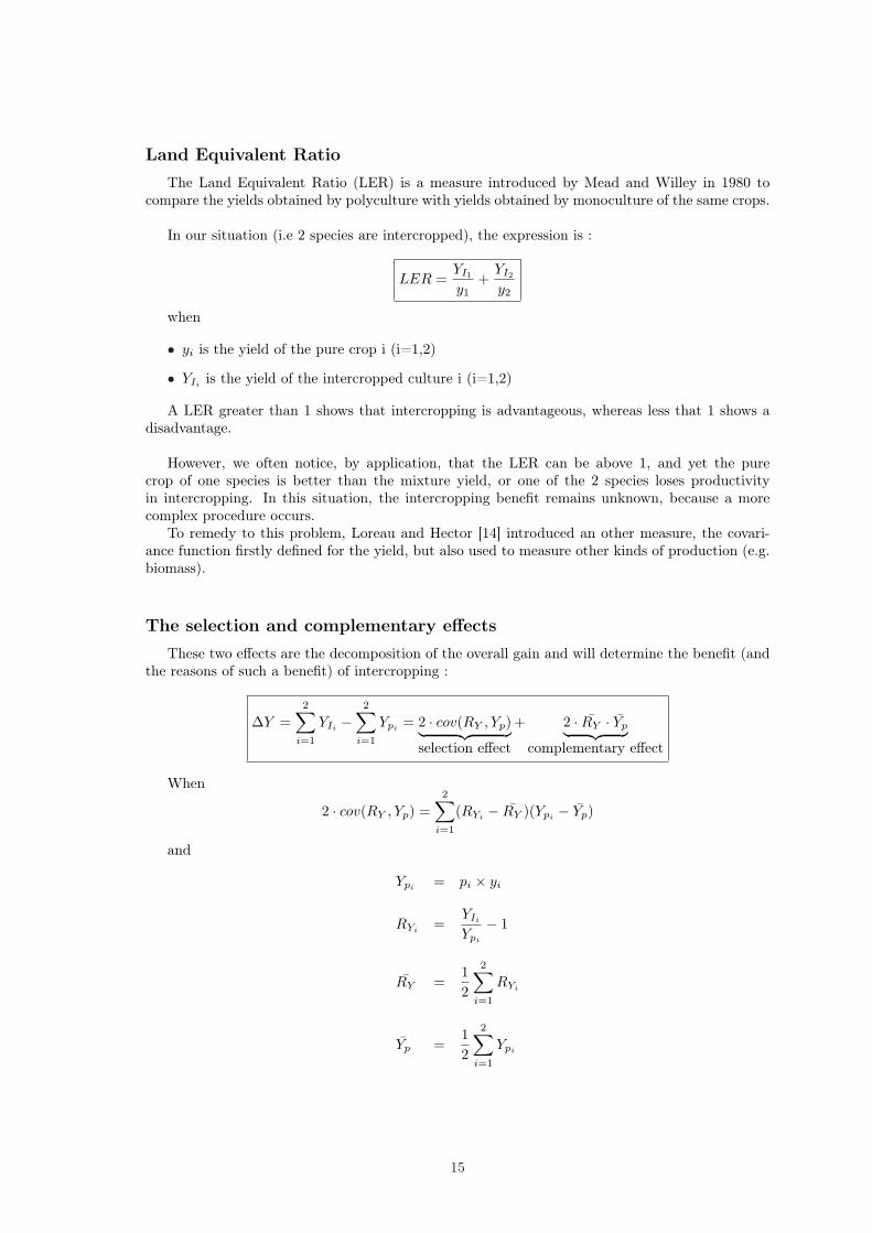
The selection and complementary effectsThese two effects are the decomposition of the overall gain and will determine the benefit (and

the reasons of such a benefit) of intercropping :

∆Y =2∑

i=1

YIi −2∑

i=1

Ypi = 2 · cov(RY , Yp)︸ ︷︷ ︸selection effect

+ 2 · RY · Yp︸ ︷︷ ︸complementary effect

When

2 · cov(RY , Yp) =2∑

i=1

(RYi − RY )(Ypi − Yp)

and

Ypi = pi × yi

RYi =YIi

Ypi

− 1

RY =12

2∑

i=1

RYi

Yp =12

2∑

i=1

Ypi

15

• Ypi is the crop monoculture yield of the ith species in the seed proportion pi , correspondingto the seed proportion used in the intercropping for this species ;

• YIiis the crop yield obtained for the ith species when 2 species are cultivated as a mixture;

• yi represents the crop yield per unit area.

The covariance function, up to a constant, is also called the selection effect because, compara-ble to 0, a high value (positive or negative) means the intercropping is favorable for one of the 2culture, but not for the other : it predicts a dominance of one of the species on the other in themixture, as if the selection of a specific species had influenced the intercrop yield.

Because the mean of two yields is always positive, the complementary effect sign depends on

RY , so the interpretation of this quantity is linked to the ratiointercrop yieldpure yield

, considering the

proportion used in the intercropping : If this quantity is widely positive, the intercropping is ageneral benefit, as if cultures stimulate each other, whereas a widely negative value means a realdisadvantage of such a combination.

If the effects are both positive, intercropping has benefit on production, and it could be dueto dominance (resp. competition) if the selection effect (resp. the complementary effect) is higherthan the complementary effect (resp. the selection effect).If the effects are both negative, both cultures are more efficient in monocrop, and there is no dom-inance species to make increase the yield.If the effects have opposite signs, we can conclude to either a large dominance (resp. an goodcomplementarity) if the selection effect (resp. the complementary effect) is widely positive or anon-benefit of intercropping if the selection effect is slightly positive and the complementary onewidely negative.

We will choose to study the 3 recounted effects (considering 2 are linked) and give the appro-priate interpretation in the following.

16

Chapter 3

Data description

3.1 The dataThe data currently consists of 10 papers composed of 2 to 32 mixtures. Each mixture is com-

posed of 4 yields, necessary to calculate the effect measures. In a word, it means that a effectmeasure does not correspond to a single study, as it is usually the case, but in a single study,several measures are carried out.

For each mixture, we want to study 3 effect measures, the LER index, the selection effect andthe complementary effect. These 2 last measures will be analyzed together, because their generaltendency will be compared for the interpretation.

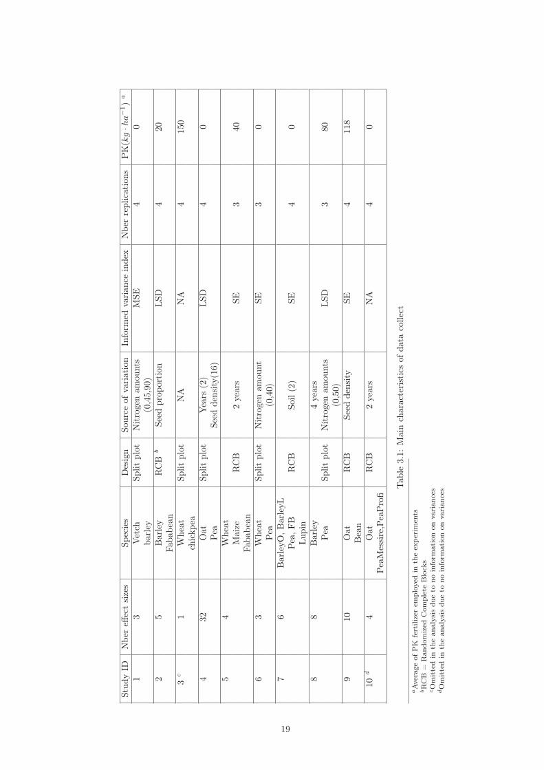
The source of variation within studies can be due to the difference of seed densities used inmixtures, the experiment years, the location (sandy loam soil or sandy soil) or the difference ofnitrogen amount used, mentioned in the database.

Details are shown in the table 3.1. The study numbers mentioned in the following analysis willalways correspond to the identifiers of this table.

A quick statistical description allows to see the main data characteristics and this also bringsus some ideas for the following work.

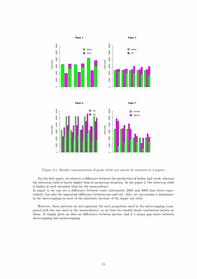
3.2 Descriptive StatisticsThe most usual is to represent the grain yield of each species for monocropping and intercrop-

ping for each mixture and each study.Through these plots, we can easily compare the species yields in monoculture, then the yields inmonoculture and intercropping.

The following representation concerns the first and the second papers, where the nitrogenamount and the seed density (resp.) are the sources of variation. The other representations are apart of the paper 4, composed of 32 mixtures, which source of variation is year (2002 and 2003)and the seed proportion used for intercropping, and a part of paper 7, which variation comes fromthe soil type and legume species.

17

Paper 1

Gra

in y

ield

010

0020

0030

0040

0050

0060

00

barley

vetch

Paper 2

Gra

in y

ield

010

0020

0030

0040

0050

0060

00

barley

FB

Paper 4

Gra

in y

ield

010

0020

0030

0040

0050

0060

00 oat

pea

Paper 7G

rain

yie

ld

010

0020

0030

0040

0050

0060

00 cereals

legume

Figure 3.1: Barplot representation of grain yields per species & mixtures in 4 papers

For the first paper, we observe a difference between the production of barley and vetch, whereasthe intercrop yield is barely higher than in monocrop situation. In the paper 2, the intercrop yieldis higher in each situation than for the monoculture.In paper 4, we can see a difference between years (alternately 2002 and 2003 have been repre-sented), but also the important difference between pea and oat. Also, we can assume a dominancein the intercropping in most of the mixtures, because of the larger oat yield.

However, these patterns do not represent the seed proportion used in the intercropping (com-pared with the one used in the monoculture), so we have be careful about conclusions drawn onthem. It simply gives an idea on differences between species, and if a major gap exists betweenintercropping and monocropping.

18

Stud

yID

Nbe

reff

ectsizes

Species

Design

Source

ofvariation

Inform

edvarian

ceindex

Nbe

rreplications

PK(k

g·h

a−

1)a

13

Vetch

Split

plot

Nitrogenam

ounts

MSE

40

barley

(0,45,90)

25

Barley

RCB

bSeed

prop

ortion

LSD

420

Faba

bean

3c

1W

heat

Split

plot

NA

NA

4150

chickp

ea4

32Oat

Split

plot

Years

(2)

LSD

40

Pea

Seed

density(16)

54

Wheat

Maize

RCB

2years

SE3

40Fa

babe

an6

3W

heat

Split

plot

Nitrogenam

ount

SE3

0Pea

(0,40)

76

BarleyO

,BarleyL

Pea,F

BRCB

Soil(2)

SE4

0Lu

pin

88

Barley

4years

Pea

Split

plot

Nitrogenam

ounts

LSD

380

(0,50)

910

Oat

RCB

Seed

density

SE4

118

Bean

10d

4Oat

RCB

2years

NA

40

PeaMessire,PeaProfi

Tab

le3.1:

Maincharacteristicsof

data

collect

aAverage

ofPK

fertilizerem

ployed

intheexpe

riments

bRCB

=Ran

domized

Com

pleteBlocks

cOmittedin

thean

alysis

dueto

noinform

ationon

varian

ces

dOmittedin

thean

alysis

dueto

noinform

ationon

varian

ces

19

Chapter 4

Meta analysis : First approach

For this first part, we will assume mixtures as if they were independent. Moreover, the varianceattributed to each mixture (and by consequence the weight) is extracted from the ANOVA tablessupplied by the articles.

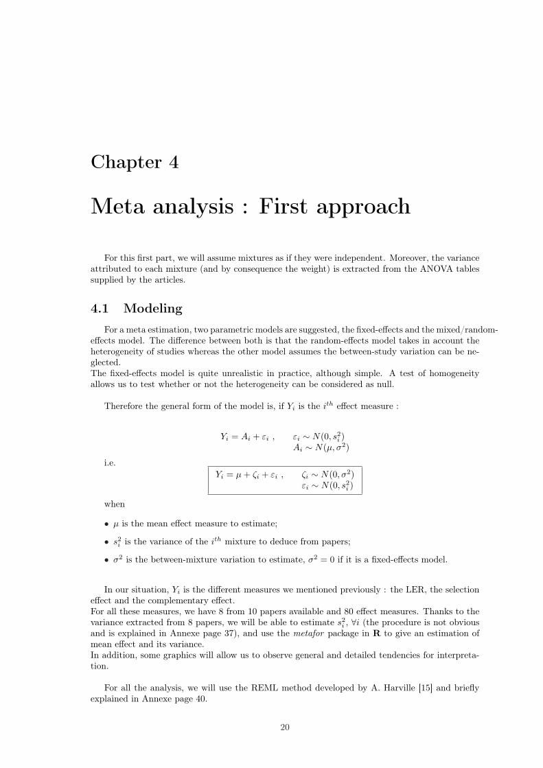
4.1 ModelingFor a meta estimation, two parametric models are suggested, the fixed-effects and the mixed/random-

effects model. The difference between both is that the random-effects model takes in account theheterogeneity of studies whereas the other model assumes the between-study variation can be ne-glected.The fixed-effects model is quite unrealistic in practice, although simple. A test of homogeneityallows us to test whether or not the heterogeneity can be considered as null.

Therefore the general form of the model is, if Yi is the ith effect measure :

Yi = Ai + εi , εi ∼ N(0, s2i )

Ai ∼ N(µ, σ2)

i.e.Yi = µ + ζi + εi , ζi ∼ N(0, σ2)

εi ∼ N(0, s2i )

when

• µ is the mean effect measure to estimate;

• s2i is the variance of the ith mixture to deduce from papers;

• σ2 is the between-mixture variation to estimate, σ2 = 0 if it is a fixed-effects model.

In our situation, Yi is the different measures we mentioned previously : the LER, the selectioneffect and the complementary effect.For all these measures, we have 8 from 10 papers available and 80 effect measures. Thanks to thevariance extracted from 8 papers, we will be able to estimate s2

i , ∀i (the procedure is not obviousand is explained in Annexe page 37), and use the metafor package in R to give an estimation ofmean effect and its variance.In addition, some graphics will allow us to observe general and detailed tendencies for interpreta-tion.

For all the analysis, we will use the REML method developed by A. Harville [15] and brieflyexplained in Annexe page 40.

20

4.2 The LER effect measure

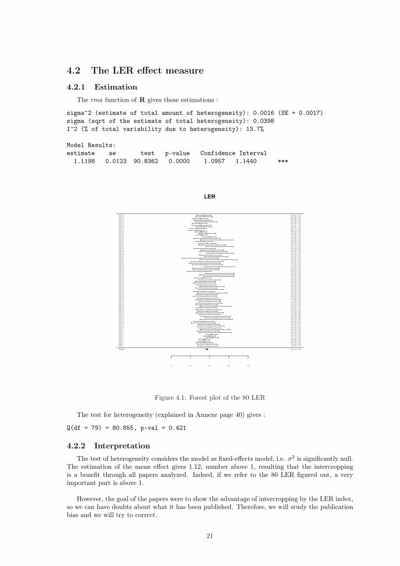
4.2.1 EstimationThe rma function of R gives these estimations :

sigma^2 (estimate of total amount of heterogeneity): 0.0016 (SE = 0.0017)sigma (sqrt of the estimate of total heterogeneity): 0.0398I^2 (% of total variability due to heterogeneity): 13.7%

Model Results:estimate se test p-value Confidence Interval1.1198 0.0123 90.8362 0.0000 1.0957 1.1440 ***

LER

1.12 [ 1.10 , 1.14 ]RE Model

0.4 0.78 1.17 1.56 1.94

Study 1Study 2Study 3Study 4Study 5Study 6Study 7Study 8Study 9Study 10Study 11Study 12Study 13Study 14Study 15Study 16Study 17Study 18Study 19Study 20Study 21Study 22Study 23Study 24Study 25Study 26Study 27Study 28Study 29Study 30Study 31Study 32Study 33Study 34Study 35Study 36Study 37Study 38Study 39Study 40Study 41Study 42Study 43Study 44Study 45Study 46Study 47Study 48Study 49Study 50Study 51Study 52Study 53Study 54Study 55Study 56Study 57Study 58Study 59Study 60Study 61Study 62Study 63Study 64Study 65Study 66Study 67Study 68Study 69Study 70Study 71Study 72Study 73Study 74Study 75Study 76Study 77Study 78Study 79Study 80

1.14 [ 0.94 , 1.34 ] 1.13 [ 0.93 , 1.33 ] 1.06 [ 0.90 , 1.22 ] 1.06 [ 0.94 , 1.18 ] 1.08 [ 0.96 , 1.19 ] 1.23 [ 1.11 , 1.34 ] 1.17 [ 1.06 , 1.28 ] 1.21 [ 1.10 , 1.32 ] 1.28 [ 0.96 , 1.61 ] 1.15 [ 0.93 , 1.37 ] 1.28 [ 0.99 , 1.58 ] 1.17 [ 0.95 , 1.40 ] 1.20 [ 0.93 , 1.47 ] 1.16 [ 0.95 , 1.37 ] 1.05 [ 0.81 , 1.30 ] 1.06 [ 0.85 , 1.27 ] 1.30 [ 0.98 , 1.63 ] 1.33 [ 1.08 , 1.58 ] 1.30 [ 1.00 , 1.59 ] 1.17 [ 0.95 , 1.38 ] 1.17 [ 0.90 , 1.44 ] 1.13 [ 0.93 , 1.33 ] 1.15 [ 0.90 , 1.40 ] 1.11 [ 0.91 , 1.31 ] 1.29 [ 0.98 , 1.60 ] 1.11 [ 0.90 , 1.33 ] 1.16 [ 0.90 , 1.43 ] 1.17 [ 0.95 , 1.39 ] 1.14 [ 0.89 , 1.39 ] 1.14 [ 0.93 , 1.34 ] 1.08 [ 0.84 , 1.31 ] 1.12 [ 0.92 , 1.33 ] 1.22 [ 0.93 , 1.51 ] 1.06 [ 0.85 , 1.28 ] 1.19 [ 0.94 , 1.45 ] 1.10 [ 0.89 , 1.32 ] 1.22 [ 0.98 , 1.47 ] 1.10 [ 0.90 , 1.30 ] 1.07 [ 0.85 , 1.29 ] 1.09 [ 0.89 , 1.29 ] 1.17 [ 0.95 , 1.40 ] 1.04 [ 0.87 , 1.20 ] 1.36 [ 1.05 , 1.66 ] 1.32 [ 0.97 , 1.66 ] 1.38 [ 1.09 , 1.67 ] 0.96 [ 0.72 , 1.21 ] 1.10 [ 0.85 , 1.36 ] 1.10 [ 0.84 , 1.36 ] 1.37 [ 1.06 , 1.68 ] 1.13 [ 0.82 , 1.43 ] 1.08 [ 0.77 , 1.39 ] 1.12 [ 0.80 , 1.44 ] 1.35 [ 0.97 , 1.72 ] 0.98 [ 0.62 , 1.35 ] 1.31 [ 1.07 , 1.54 ] 1.19 [ 0.96 , 1.42 ] 1.38 [ 1.11 , 1.65 ] 1.24 [ 0.97 , 1.52 ] 1.22 [ 1.00 , 1.45 ] 1.07 [ 0.86 , 1.29 ] 1.37 [ 1.10 , 1.65 ] 1.22 [ 0.95 , 1.50 ] 1.13 [ 0.95 , 1.31 ] 1.06 [ 0.90 , 1.23 ] 1.31 [ 0.99 , 1.63 ] 1.12 [ 0.85 , 1.38 ] 1.17 [ 1.04 , 1.30 ] 1.02 [ 0.91 , 1.12 ] 1.13 [ 0.96 , 1.29 ] 1.00 [ 0.89 , 1.12 ] 0.90 [ 0.75 , 1.06 ] 0.94 [ 0.78 , 1.10 ] 1.06 [ 0.91 , 1.21 ] 1.01 [ 0.82 , 1.20 ] 0.97 [ 0.82 , 1.13 ] 1.11 [ 0.90 , 1.32 ] 1.04 [ 0.86 , 1.21 ] 0.98 [ 0.83 , 1.14 ] 1.06 [ 0.89 , 1.23 ] 1.06 [ 0.91 , 1.20 ]

Figure 4.1: Forest plot of the 80 LER

The test for heterogeneity (explained in Annexe page 40) gives :

Q(df = 79) = 80.855, p-val = 0.421

4.2.2 InterpretationThe test of heterogeneity considers the model as fixed-effects model, i.e. σ2 is significantly null.

The estimation of the mean effect gives 1.12, number above 1, resulting that the intercroppingis a benefit through all papers analyzed. Indeed, if we refer to the 80 LER figured out, a veryimportant part is above 1.

However, the goal of the papers were to show the advantage of intercropping by the LER index,so we can have doubts about what it has been published. Therefore, we will study the publicationbias and we will try to correct.

21

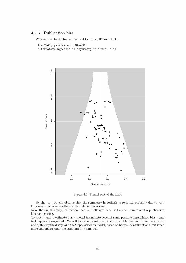
4.2.3 Publication biasWe can refer to the funnel plot and the Kendall’s rank test :

T = 2241, p-value = 1.384e-08alternative hypothesis: asymmetry in funnel plot

Observed Outcome

Sta

ndar

d E

rror

0.19

10.

143

0.09

60.

048

0.00

0

0.8 1.0 1.2 1.4 1.6

Figure 4.2: Funnel plot of the LER

By the test, we can observe that the symmetry hypothesis is rejected, probably due to veryhigh measures, whereas the standard deviation is small.Nevertheless, this empirical method can be challenged because they sometimes omit a publicationbias yet existing.To spot it and to estimate a new model taking into account some possible unpublished bias, sometechniques are suggested : We will focus on two of them, the trim and fill method, a non parametricand quite empirical way, and the Copas selection model, based on normality assumptions, but muchmore elaborated than the trim and fill technique.

22

The Trim and fill method

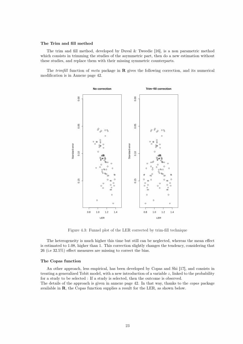
The trim and fill method, developed by Duval & Tweedie [16], is a non parametric methodwhich consists in trimming the studies of the asymmetric part, then do a new estimation withoutthese studies, and replace them with their missing symmetric counterparts.

The trimfill function of meta package in R gives the following correction, and its numericalmodification is in Annexe page 42.

0.8 1.0 1.2 1.4

0.15

0.10

0.05

0.00

No correction

LER

Sta

ndar

d er

ror

0.8 1.0 1.2 1.4

0.15

0.10

0.05

0.00

Trim−fill correction

LER

Sta

ndar

d er

ror

Figure 4.3: Funnel plot of the LER corrected by trim-fill technique

The heterogeneity is much higher this time but still can be neglected, whereas the mean effectis estimated to 1.08, higher than 1. This correction slightly changes the tendency, considering that26 (i.e 32.5%) effect measures are missing to correct the bias.

The Copas function

An other approach, less empirical, has been developed by Copas and Shi [17], and consists intreating a generalized Tobit model, with a new introduction of a variable z, linked to the probabilityfor a study to be selected : If a study is selected, then the outcome is observed.The details of the approach is given in annexe page 42. In that way, thanks to the copas packageavailable in R, the Copas function supplies a result for the LER, as shown below.

23

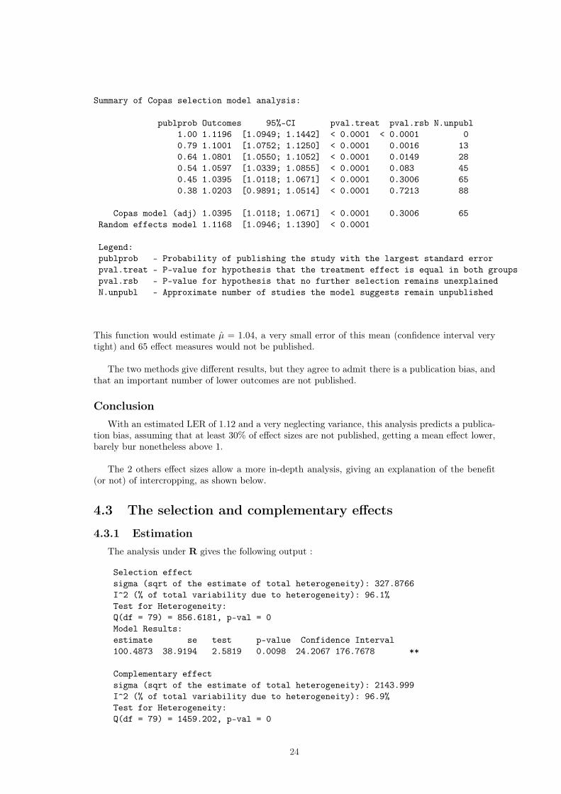
Summary of Copas selection model analysis:

publprob Outcomes 95%-CI pval.treat pval.rsb N.unpubl1.00 1.1196 [1.0949; 1.1442] < 0.0001 < 0.0001 00.79 1.1001 [1.0752; 1.1250] < 0.0001 0.0016 130.64 1.0801 [1.0550; 1.1052] < 0.0001 0.0149 280.54 1.0597 [1.0339; 1.0855] < 0.0001 0.083 450.45 1.0395 [1.0118; 1.0671] < 0.0001 0.3006 650.38 1.0203 [0.9891; 1.0514] < 0.0001 0.7213 88

Copas model (adj) 1.0395 [1.0118; 1.0671] < 0.0001 0.3006 65Random effects model 1.1168 [1.0946; 1.1390] < 0.0001

Legend:publprob - Probability of publishing the study with the largest standard errorpval.treat - P-value for hypothesis that the treatment effect is equal in both groupspval.rsb - P-value for hypothesis that no further selection remains unexplainedN.unpubl - Approximate number of studies the model suggests remain unpublished

This function would estimate µ = 1.04, a very small error of this mean (confidence interval verytight) and 65 effect measures would not be published.

The two methods give different results, but they agree to admit there is a publication bias, andthat an important number of lower outcomes are not published.

ConclusionWith an estimated LER of 1.12 and a very neglecting variance, this analysis predicts a publica-

tion bias, assuming that at least 30% of effect sizes are not published, getting a mean effect lower,barely bur nonetheless above 1.

The 2 others effect sizes allow a more in-depth analysis, giving an explanation of the benefit(or not) of intercropping, as shown below.

4.3 The selection and complementary effects

4.3.1 EstimationThe analysis under R gives the following output :

Selection effectsigma (sqrt of the estimate of total heterogeneity): 327.8766I^2 (% of total variability due to heterogeneity): 96.1%Test for Heterogeneity:Q(df = 79) = 856.6181, p-val = 0Model Results:estimate se test p-value Confidence Interval100.4873 38.9194 2.5819 0.0098 24.2067 176.7678 **

Complementary effectsigma (sqrt of the estimate of total heterogeneity): 2143.999I^2 (% of total variability due to heterogeneity): 96.9%Test for Heterogeneity:Q(df = 79) = 1459.202, p-val = 0

24

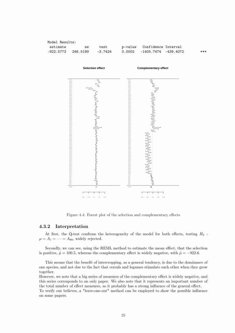
Model Results:estimate se test p-value Confidence Interval-922.5773 246.5199 -3.7424 0.0002 -1405.7474 -439.4072 ***

Selection effect

RE Model

−4800.22 −2777.35 −754.47 1268.4 3291.28

Study 1

Study 2

Study 3

Study 4

Study 5

Study 6

Study 7

Study 8

Study 9

Study 10

Study 11

Study 12

Study 13

Study 14

Study 15

Study 16

Study 17

Study 18

Study 19

Study 20

Study 21

Study 22

Study 23

Study 24

Study 25

Study 26

Study 27

Study 28

Study 29

Study 30

Study 31

Study 32

Study 33

Study 34

Study 35

Study 36

Study 37

Study 38

Study 39

Study 40

Study 41

Study 42

Study 43

Study 44

Study 45

Study 46

Study 47

Study 48

Study 49

Study 50

Study 51

Study 52

Study 53

Study 54

Study 55

Study 56

Study 57

Study 58

Study 59

Study 60

Study 61

Study 62

Study 63

Study 64

Study 65

Study 66

Study 67

Study 68

Study 69

Study 70

Study 71

Study 72

Study 73

Study 74

Study 75

Study 76

Study 77

Study 78

Study 79

Study 80

Complementary effect

RE Model

−8209.35 −3903.02 403.32 4709.65 9015.98

Study 1

Study 2

Study 3

Study 4

Study 5

Study 6

Study 7

Study 8

Study 9

Study 10

Study 11

Study 12

Study 13

Study 14

Study 15

Study 16

Study 17

Study 18

Study 19

Study 20

Study 21

Study 22

Study 23

Study 24

Study 25

Study 26

Study 27

Study 28

Study 29

Study 30

Study 31

Study 32

Study 33

Study 34

Study 35

Study 36

Study 37

Study 38

Study 39

Study 40

Study 41

Study 42

Study 43

Study 44

Study 45

Study 46

Study 47

Study 48

Study 49

Study 50

Study 51

Study 52

Study 53

Study 54

Study 55

Study 56

Study 57

Study 58

Study 59

Study 60

Study 61

Study 62

Study 63

Study 64

Study 65

Study 66

Study 67

Study 68

Study 69

Study 70

Study 71

Study 72

Study 73

Study 74

Study 75

Study 76

Study 77

Study 78

Study 79

Study 80

Figure 4.4: Forest plot of the selection and complementary effects

4.3.2 InterpretationAt first, the Q-test confirms the heterogeneity of the model for both effects, testing H0 :

µ = A1 = · · · = A80, widely rejected.

Secondly, we can see, using the REML method to estimate the mean effect, that the selectionis positive, µ = 100.5, whereas the complementary effect is widely negative, with µ = −922.6.

This means that the benefit of intercropping, as a general tendency, is due to the dominance ofone species, and not due to the fact that cereals and legumes stimulate each other when they growtogether.However, we note that a big series of measures of the complementary effect is widely negative, andthis series corresponds to an only paper. We also note that it represents an important number ofthe total number of effect measures, so it probably has a strong influence of the general effect.To verify our believes, a "leave-one-out" method can be employed to show the possible influenceon some papers.

25

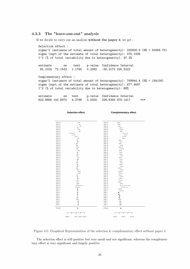
4.3.3 The "leave-one-out" analysisIf we decide to carry out an analysis without the paper 4, we get :

Selection effect :sigma^2 (estimate of total amount of heterogeneity): 225808.9 (SE = 50958.75)sigma (sqrt of the estimate of total heterogeneity): 475.1936I^2 (% of total variability due to heterogeneity): 97.3%

estimate se test p-value Confidence Interval85.1024 72.1543 1.1795 0.2382 -56.3173 226.5222

Complementary effect :sigma^2 (estimate of total amount of heterogeneity): 769944.4 (SE = 194108)sigma (sqrt of the estimate of total heterogeneity): 877.4647I^2 (% of total variability due to heterogeneity): 88%

estimate se test p-value Confidence Interval602.9886 140.8970 4.2796 0.0000 326.8356 879.1417 ***

Selection effect

RE Model

−4800.22 −754.47 1268.4 3291.28

Study 1

Study 2

Study 3

Study 4

Study 5

Study 6

Study 7

Study 8

Study 9

Study 10

Study 11

Study 12

Study 13

Study 14

Study 15

Study 16

Study 17

Study 18

Study 19

Study 20

Study 21

Study 22

Study 23

Study 24

Study 25

Study 26

Study 27

Study 28

Study 29

Study 30

Study 31

Study 32

Study 33

Study 34

Study 35

Study 36

Study 37

Study 38

Study 39

Study 40

Study 41

Study 42

Study 43

Study 44

Study 45

Study 46

Study 47

Study 48

Complementary effect

RE Model

−3415.52 2400.75 8217.01

Study 1

Study 2

Study 3

Study 4

Study 5

Study 6

Study 7

Study 8

Study 9

Study 10

Study 11

Study 12

Study 13

Study 14

Study 15

Study 16

Study 17

Study 18

Study 19

Study 20

Study 21

Study 22

Study 23

Study 24

Study 25

Study 26

Study 27

Study 28

Study 29

Study 30

Study 31

Study 32

Study 33

Study 34

Study 35

Study 36

Study 37

Study 38

Study 39

Study 40

Study 41

Study 42

Study 43

Study 44

Study 45

Study 46

Study 47

Study 48

Figure 4.5: Graphical Representation of the selection & complementary effect without paper 4

The selection effect is still positive but very small and not significant, whereas the complemen-tary effect is very significant and largely positive.

26

The eliminated study has an important impact on results, but also show that it is at the origin ofa negative complementary effect.By looking at its features in the paper, we notice this is the only mixture oat+pea treated and thatall experiments from other articles received a N (and/or P and/or K) fertilizer except the studies4 and 7. However, we did not notice a particular tendency for the study 7.If we look further, we also notice that the study 4, which experiments (with different seed propor-tions tested) have been led in 2002 and 2003, had a precipitation of 338 mm the first year, but only185 mm the other year. We note that both effects are higher in 2002 than in 2003. Moreover, theannual rainfall in the paper 7 is much higher with 600 mm or 700 mm of precipitation accordingto the location.

As a consequence, we could think that a lack of commercial fertilization and rainfall has animpact on the effects, resulting a negative complementary effect, and a low positive selection effect,i.e. an inefficiency of intercropping in this context.

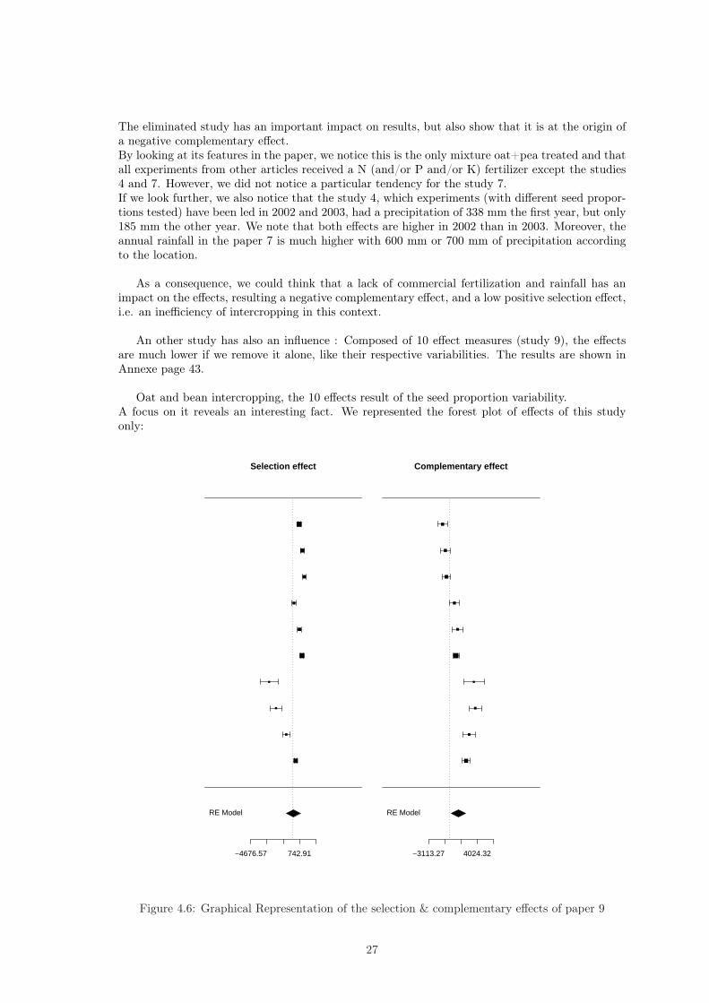
An other study has also an influence : Composed of 10 effect measures (study 9), the effectsare much lower if we remove it alone, like their respective variabilities. The results are shown inAnnexe page 43.

Oat and bean intercropping, the 10 effects result of the seed proportion variability.A focus on it reveals an interesting fact. We represented the forest plot of effects of this studyonly:

Selection effect

RE Model

−4676.57 742.91

Complementary effect

RE Model

−3113.27 4024.32

Figure 4.6: Graphical Representation of the selection & complementary effects of paper 9

27

We note 3 different tendencies, corresponding in fact to 3 different seed proportion of oat (thelowest correspond to the first represented effects). With a low seed density, the complementaryeffect is obvious, species stimulate each other.At the highest densities, there is an inverse phenomenon : oat dominates bean.

The sensitivity analysis showed influences of 2 studies, in which the lack of commercial fertil-izer and/or water, and a too important seed density provokes a lack of competition, in favour of adominance of one of the species. The use of specific cultures in intercropping may also play a roleon this phenomenon.

A publication bias is explained by the fact that some studies do not show what they have,but what they want to have. In this analysis, studies wanted to prove the benefit of intercroppingthrough the LER index and not through these double effects. For these reasons, we will not developa publication bias study for the 2 effects.

ConclusionWe notice this time a strong influence of 2 studies, the first being large, with an inefficacy

of intercropping because of a large negative complementary effect and a small positive selectioneffect, and the second with an important variability according to the proportion used to grow thedominant culture (oat). However, the other effects reveal a competition between species, then areal benefit of the intercropping practice.

So far, we did not consider effect measures were in studies, but we noticed however some studyeffects. Therefore, a variation within study and between study can be taken into account to improvethe model and our statement.

28

Chapter 5

Meta analysis : Second approach

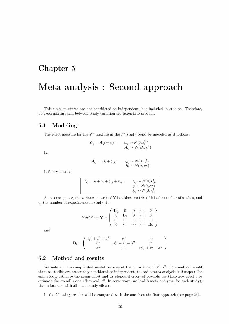
This time, mixtures are not considered as independent, but included in studies. Therefore,between-mixture and between-study variation are taken into account.

5.1 ModelingThe effect measure for the jth mixture in the ith study could be modeled as it follows :

Yij = Aij + εij , εij ∼ N(0, s2ij)

Aij ∼ N(Bi, τ2i )

i.e

Aij = Bi + ξij , ξij ∼ N(0, τ2i )

Bi ∼ N(µ, σ2)It follows that :

Yij = µ + γi + ξij + εij , εij ∼ N(0, s2ij)

γi ∼ N(0, σ2)ξij ∼ N(0, τ2

i )

As a consequence, the variance matrix of Y is a block matrix (if k is the number of studies, andni the number of experiments in study i) :

V ar(Y ) = V =

B1 0 0 · · · 00 B2 0 · · · 0· · · · · · · · · · · · · · ·0 · · · · · · · · · Bk

and

Bi =

s2i1 + τ2

i + σ2 σ2 · · ·σ2 s2

i2 + τ21 + σ2 σ2

σ2 · · · s2ini

+ τ2i + σ2

5.2 Method and resultsWe note a more complicated model because of the covariance of Y, σ2. The method would

then, as studies are reasonably considered as independent, to lead a meta analysis in 2 steps : Foreach study, estimate the mean effect and its standard error; afterwards use these new results toestimate the overall mean effect and σ2. In some ways, we lead 8 meta analysis (for each study),then a last one with all mean study effects.

In the following, results will be compared with the one from the first approach (see page 24).

29

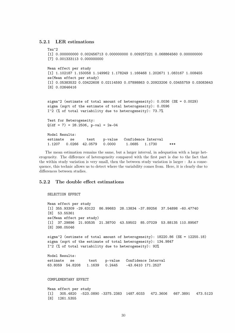
5.2.1 LER estimationsTau^2[1] 0.000000000 0.002456713 0.000000000 0.009257221 0.068864560 0.000000000[7] 0.001333113 0.000000000

Mean effect per study[1] 1.102187 1.150058 1.149962 1.178249 1.166468 1.202671 1.083167 1.008455se(Mean effect per study)[1] 0.05383532 0.03422608 0.02114593 0.07898863 0.20923206 0.03455759 0.03083643[8] 0.02646416

sigma^2 (estimate of total amount of heterogeneity): 0.0036 (SE = 0.0029)sigma (sqrt of the estimate of total heterogeneity): 0.0596I^2 (% of total variability due to heterogeneity): 73.7%

Test for Heterogeneity:Q(df = 7) = 28.2506, p-val = 2e-04

Model Results:estimate se test p-value Confidence Interval1.1207 0.0266 42.0579 0.0000 1.0685 1.1730 ***

The mean estimation remains the same, but a larger interval, in adequation with a large het-erogeneity. The difference of heterogeneity compared with the first part is due to the fact thatthe within study variation is very small, then the between study variation is larger : As a conse-quence, this technic allows us to detect where the variability comes from. Here, it is clearly due todifferences between studies.

5.2.2 The double effect estimations

SELECTION EFFECT

Mean effect per study[1] 355.93309 -29.63122 86.99683 28.13834 -37.89256 37.54898 -60.47740[8] 53.55361se(Mean effect per study)[1] 37.29896 21.93535 21.38700 43.59502 85.07029 53.88135 110.89567[8] 398.05046

sigma^2 (estimate of total amount of heterogeneity): 18220.86 (SE = 12255.18)sigma (sqrt of the estimate of total heterogeneity): 134.9847I^2 (% of total variability due to heterogeneity): 92%

Model Results:estimate se test p-value Confidence Interval63.8059 54.8208 1.1639 0.2445 -43.6410 171.2527

COMPLEMENTARY EFFECT

Mean effect per study[1] 305.4820 -523.0890 -3375.2383 1487.6033 472.3606 667.3891 473.5123[8] 1261.5355

30

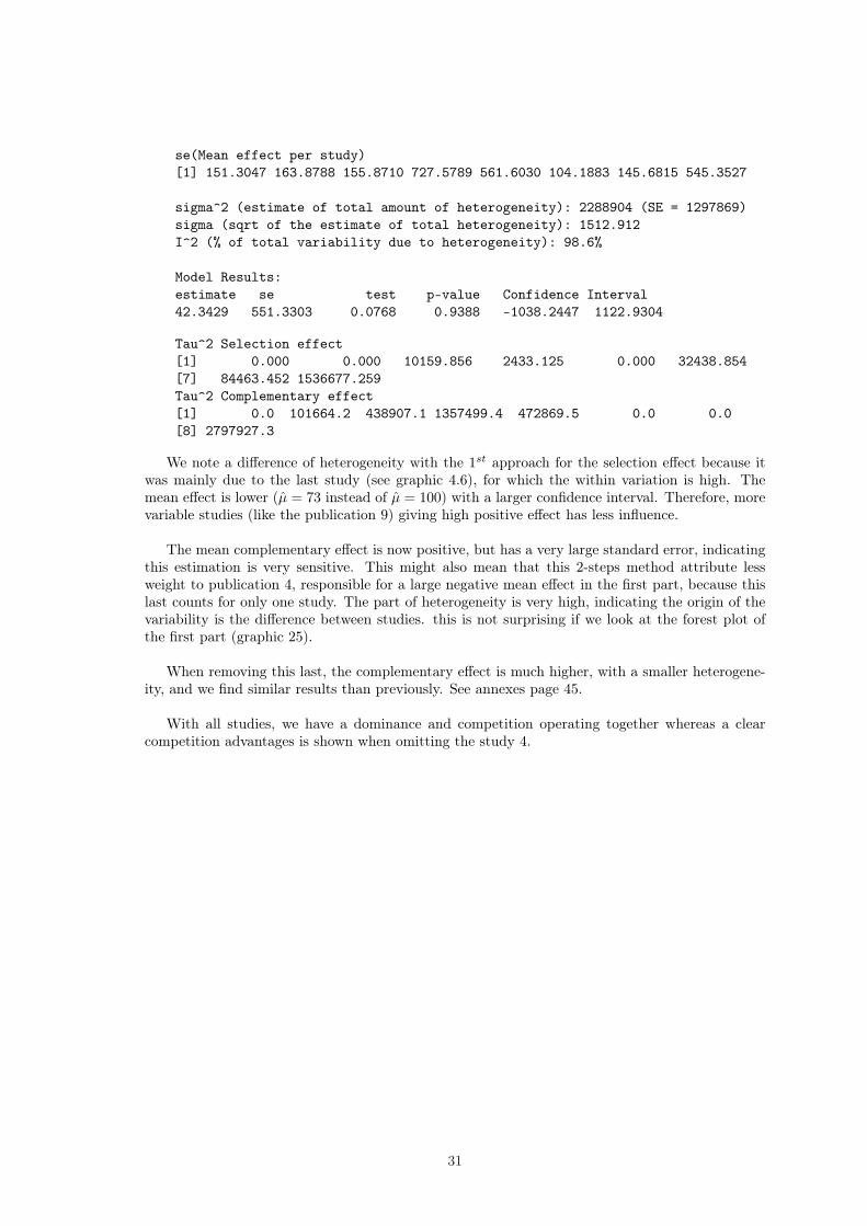
se(Mean effect per study)[1] 151.3047 163.8788 155.8710 727.5789 561.6030 104.1883 145.6815 545.3527

sigma^2 (estimate of total amount of heterogeneity): 2288904 (SE = 1297869)sigma (sqrt of the estimate of total heterogeneity): 1512.912I^2 (% of total variability due to heterogeneity): 98.6%

Model Results:estimate se test p-value Confidence Interval42.3429 551.3303 0.0768 0.9388 -1038.2447 1122.9304

Tau^2 Selection effect[1] 0.000 0.000 10159.856 2433.125 0.000 32438.854[7] 84463.452 1536677.259Tau^2 Complementary effect[1] 0.0 101664.2 438907.1 1357499.4 472869.5 0.0 0.0[8] 2797927.3

We note a difference of heterogeneity with the 1st approach for the selection effect because itwas mainly due to the last study (see graphic 4.6), for which the within variation is high. Themean effect is lower (µ = 73 instead of µ = 100) with a larger confidence interval. Therefore, morevariable studies (like the publication 9) giving high positive effect has less influence.

The mean complementary effect is now positive, but has a very large standard error, indicatingthis estimation is very sensitive. This might also mean that this 2-steps method attribute lessweight to publication 4, responsible for a large negative mean effect in the first part, because thislast counts for only one study. The part of heterogeneity is very high, indicating the origin of thevariability is the difference between studies. this is not surprising if we look at the forest plot ofthe first part (graphic 25).

When removing this last, the complementary effect is much higher, with a smaller heterogene-ity, and we find similar results than previously. See annexes page 45.

With all studies, we have a dominance and competition operating together whereas a clearcompetition advantages is shown when omitting the study 4.

31

Conclusion

From the classical method to a more elaborated model, the approaches dealt with 3 effect sizesto give different perspectives to a single question : Has intercropping got benefic effects on grainyields ?

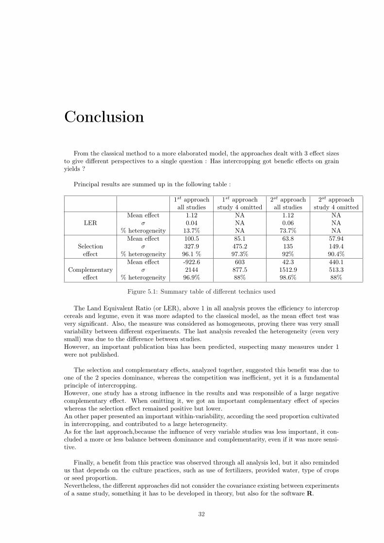
Principal results are summed up in the following table :

1st approach 1st approach 2st approach 2st approachall studies study 4 omitted all studies study 4 omitted

Mean effect 1.12 NA 1.12 NALER σ 0.04 NA 0.06 NA

% heterogeneity 13.7% NA 73.7% NAMean effect 100.5 85.1 63.8 57.94

Selection σ 327.9 475.2 135 149.4effect % heterogeneity 96.1 % 97.3% 92% 90.4%

Mean effect -922.6 603 42.3 440.1Complementary σ 2144 877.5 1512.9 513.3

effect % heterogeneity 96.9% 88% 98.6% 88%

Figure 5.1: Summary table of different technics used

The Land Equivalent Ratio (or LER), above 1 in all analysis proves the efficiency to intercropcereals and legume, even it was more adapted to the classical model, as the mean effect test wasvery significant. Also, the measure was considered as homogeneous, proving there was very smallvariability between different experiments. The last analysis revealed the heterogeneity (even verysmall) was due to the difference between studies.However, an important publication bias has been predicted, suspecting many measures under 1were not published.

The selection and complementary effects, analyzed together, suggested this benefit was due toone of the 2 species dominance, whereas the competition was inefficient, yet it is a fundamentalprinciple of intercropping.However, one study has a strong influence in the results and was responsible of a large negativecomplementary effect. When omitting it, we got an important complementary effect of specieswhereas the selection effect remained positive but lower.An other paper presented an important within-variability, according the seed proportion cultivatedin intercropping, and contributed to a large heterogeneity.As for the last approach,because the influence of very variable studies was less important, it con-cluded a more or less balance between dominance and complementarity, even if it was more sensi-tive.

Finally, a benefit from this practice was observed through all analysis led, but it also remindedus that depends on the culture practices, such as use of fertilizers, provided water, type of cropsor seed proportion.Nevertheless, the different approaches did not consider the covariance existing between experimentsof a same study, something it has to be developed in theory, but also for the software R.

32

Personal OutcomeI was hesitant to go there because the subject was quite hard, I had never met my supervisor,

and it was not a English-speaking country. But I like challenges, so I decided to spent my summerthere for a new adventure.Danes speak very well English, so the language was not a problem, my supervisor is a very nice per-son and this experience brought me much more than expected in terms of relationships and culture.

As for the subject, it was obscure at first because my work consisted in doing a meta analysis,something I did not know, but the project was really interesting, exactly the kind of topic I wantedto deal with : By proving that farming practices can be an advantage for people and Environmentprotection, my work would contribute to bring concrete solutions for the sustainable development.

From meta analysis to biodiversity and Agriculture, I improved my knowledge and it gave meclearer ideas of my future career, and what I should expect when confronting data in real context.

33

34

Annexes

35

36

Preliminaries

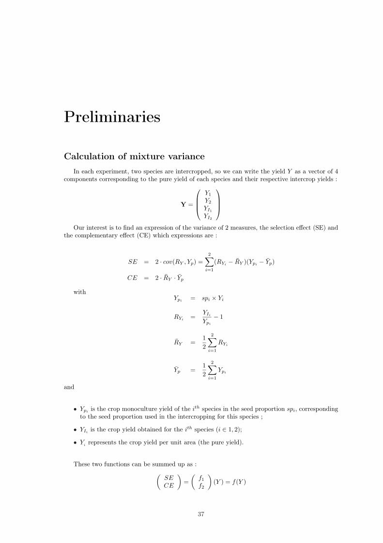
Calculation of mixture varianceIn each experiment, two species are intercropped, so we can write the yield Y as a vector of 4

components corresponding to the pure yield of each species and their respective intercrop yields :

Y =

Y1

Y2

YI1

YI2

Our interest is to find an expression of the variance of 2 measures, the selection effect (SE) andthe complementary effect (CE) which expressions are :

SE = 2 · cov(RY , Yp) =2∑

i=1

(RYi − RY )(Ypi − Yp)

CE = 2 · RY · Yp

withYpi = spi × Yi

RYi =YIi

Ypi

− 1

RY =12

2∑

i=1

RYi

Yp =12

2∑

i=1

Ypi

and

• Ypi is the crop monoculture yield of the ith species in the seed proportion spi, correspondingto the seed proportion used in the intercropping for this species ;

• YIi is the crop yield obtained for the ith species (i ∈ 1, 2);

• Yi represents the crop yield per unit area (the pure yield).

These two functions can be summed up as :(

SECE

)=

(f1

f2

)(Y ) = f(Y )

37

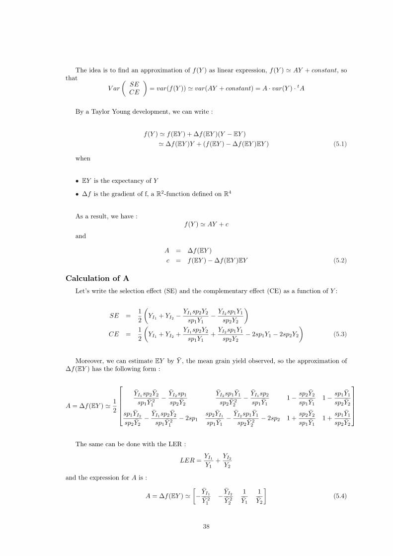
The idea is to find an approximation of f(Y ) as linear expression, f(Y ) ' AY + constant, sothat

V ar

(SECE

)= var(f(Y )) ' var(AY + constant) = A · var(Y ) · tA

By a Taylor Young development, we can write :

f(Y ) ' f(EY ) + ∆f(EY )(Y − EY )' ∆f(EY )Y + (f(EY )−∆f(EY )EY ) (5.1)

when

• EY is the expectancy of Y

• ∆f is the gradient of f, a R2-function defined on R4

As a result, we have :f(Y ) ' AY + c

and

A = ∆f(EY )c = f(EY )−∆f(EY )EY (5.2)

Calculation of ALet’s write the selection effect (SE) and the complementary effect (CE) as a function of Y :

SE =12

(YI1 + YI2 −

YI1sp2Y2

sp1Y1− YI2sp1Y1

sp2Y2

)

CE =12

(YI1 + YI2 +

YI1sp2Y2

sp1Y1+

YI2sp1Y1

sp2Y2− 2sp1Y1 − 2sp2Y2

)(5.3)

Moreover, we can estimate EY by Y , the mean grain yield observed, so the approximation of∆f(EY ) has the following form :

A = ∆f(EY ) ' 12

YI1sp2Y2

sp1Y 21

− YI2sp1

sp2Y2

YI2sp1Y1

sp2Y 22

− YI1sp2

sp1Y11− sp2Y2

sp1Y11− sp1Y1

sp2Y2

sp1YI2

sp2Y2− YI1sp2Y2

sp1Y 21

− 2sp1sp2YI1

sp1Y1− YI2sp1Y1

sp2Y 22

− 2sp2 1 +sp2Y2

sp1Y11 +

sp1Y1

sp2Y2

The same can be done with the LER :

LER =YI1

Y1+

YI2

Y2

and the expression for A is :

A = ∆f(EY ) '[− YI1

Y 21

− YI2

Y 22

1Y1

1Y2

](5.4)

38

For each experiment, we can easily calculate A with R and its transposed matrix.

Now, we have to express the variance-covariance matrix of Y with the variance measures sup-plied by the studies.Indeed, the analysis of variance carried out for each study allows us to make a reasonable approx-imation of var(Y ).

Use of analysis of varianceThe publications provide several variance index enumerated below :

1. The Mean Square Error (MSE) of an experimentUnder conditions of normality and independency,

MSE = σ2

2. The coefficient of variation (CV) for each speciesIt is defined as the ratio of the standard deviation σ to the mean µ :

Cv =σ

µ

3. The Standard Error (SE)of the meanIt is defined as the ratio of σ to the sample size square root :

SE =σ√n

4. The Least Significant Difference (LSD)The expression is :

LSD = σ · t1−α2·√

2n

• The LSD is used to compare several groups, so n corresponds to the number of obser-vations contained in each group (this number must be the same for each group);

• t1−α2is the quantile value with the degree of freedom of the error. It is reasonable to

approximate it by 2;• α is the test level (usually α = 5%).

Some assumptions can be deduced by studies, and others are assumed to figure out V ar(Y ).

1. Due to lack of information, we assume cov(Ya, Yb) = 0, ∀a 6= b

2. var(Y1) = var(YI1) and var(Y2) = var(YI2)

3. In case of mean yields provided for each level of a factor (e.g. 3 different nitrogen amountsused as fertilizer), var(Yi,N1) = var(Yi,N2) = var(Yi,N3), ∀i ∈ {1, 2}

As the yields obtained correspond to the mean yields (we don’t have the original data) of yieldsfrom a number of combinations_ let’s say m combinations _ we have, for example for Y1 :

39

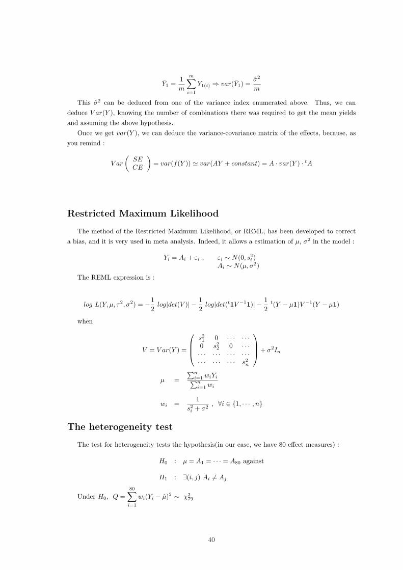
Y1 =1m

m∑

i=1

Y1(i) ⇒ var(Y1) =σ2

m

This σ2 can be deduced from one of the variance index enumerated above. Thus, we candeduce V ar(Y ), knowing the number of combinations there was required to get the mean yieldsand assuming the above hypothesis.

Once we get var(Y ), we can deduce the variance-covariance matrix of the effects, because, asyou remind :

V ar

(SECE

)= var(f(Y )) ' var(AY + constant) = A · var(Y ) · tA

Restricted Maximum Likelihood

The method of the Restricted Maximum Likelihood, or REML, has been developed to correcta bias, and it is very used in meta analysis. Indeed, it allows a estimation of µ, σ2 in the model :

Yi = Ai + εi , εi ∼ N(0, s2i )

Ai ∼ N(µ, σ2)

The REML expression is :

log L(Y, µ, τ2, σ2) = −12

log|det(V )| − 12

log|det(t1V −11)| − 12

t(Y − µ1)V −1(Y − µ1)

when

V = V ar(Y ) =

s21 0 · · · · · ·0 s2

2 0 · · ·· · · · · · · · · · · ·· · · · · · · · · s2

n

+ σ2In

µ =∑n

i=1 wiYi∑ni=1 wi

wi =1

s2i + σ2

, ∀i ∈ {1, · · · , n}

The heterogeneity test

The test for heterogeneity tests the hypothesis(in our case, we have 80 effect measures) :

H0 : µ = A1 = · · · = A80 against

H1 : ∃(i, j) Ai 6= Aj

Under H0, Q =80∑

i=1

wi(Yi − µ)2 ∼ χ279

40

where

µ =∑80

i=1 wiYi∑80i=1 wi

wi =1s2

i

If the p-value is under the significative level α (usually 0.05), the hypothesis H0 is rejected,so we can not talk about homogeneity, i.e there is a significant difference between mixture effects,therefore a between-mixture variation has to be considered; thus σ2, the between-study variationis significantly different from 0.

41

Meta analysis : First approach

LER

The trim and fill method

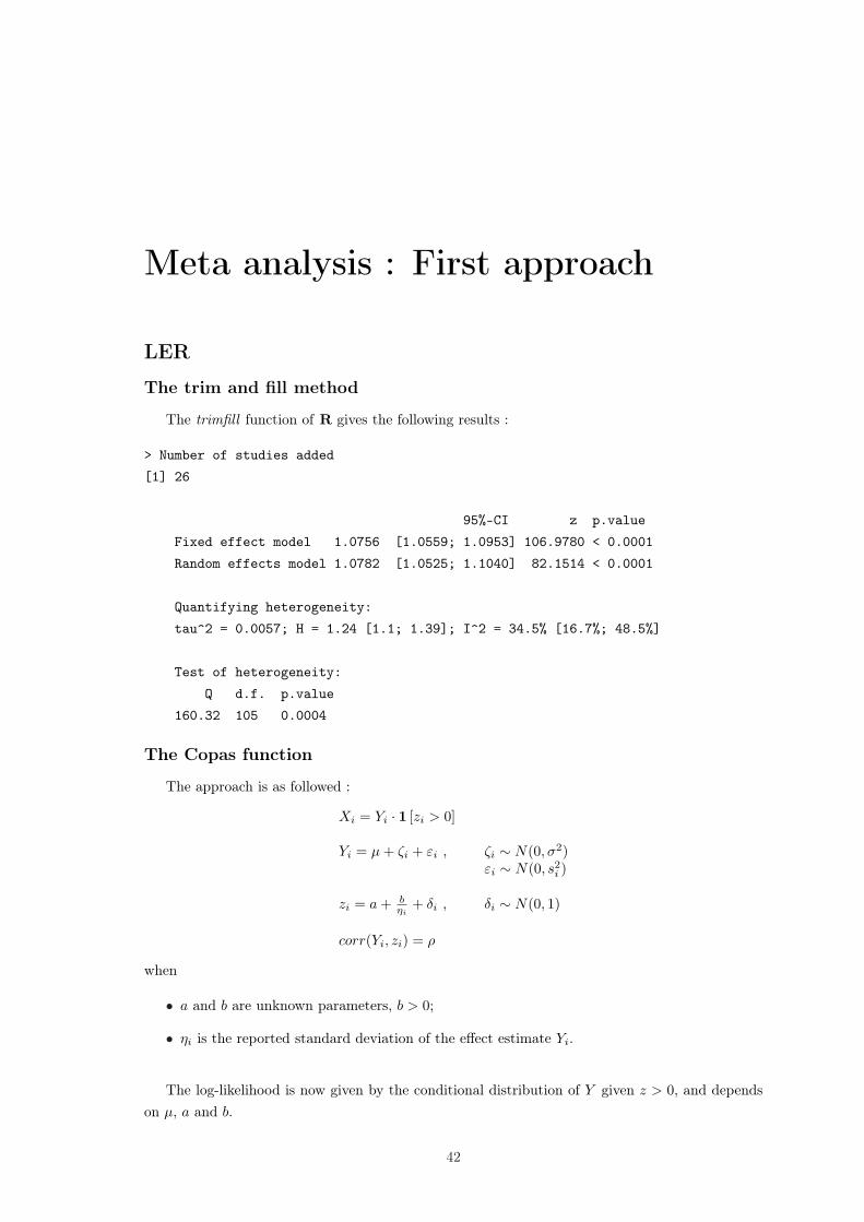
The trimfill function of R gives the following results :

> Number of studies added

[1] 26

95%-CI z p.value

Fixed effect model 1.0756 [1.0559; 1.0953] 106.9780 < 0.0001

Random effects model 1.0782 [1.0525; 1.1040] 82.1514 < 0.0001

Quantifying heterogeneity:

tau^2 = 0.0057; H = 1.24 [1.1; 1.39]; I^2 = 34.5% [16.7%; 48.5%]

Test of heterogeneity:

Q d.f. p.value

160.32 105 0.0004

The Copas function

The approach is as followed :

Xi = Yi · 1 [zi > 0]

Yi = µ + ζi + εi , ζi ∼ N(0, σ2)εi ∼ N(0, s2

i )

zi = a + bηi

+ δi , δi ∼ N(0, 1)

corr(Yi, zi) = ρ

when

• a and b are unknown parameters, b > 0;

• ηi is the reported standard deviation of the effect estimate Yi.

The log-likelihood is now given by the conditional distribution of Y given z > 0, and dependson µ, a and b.

42

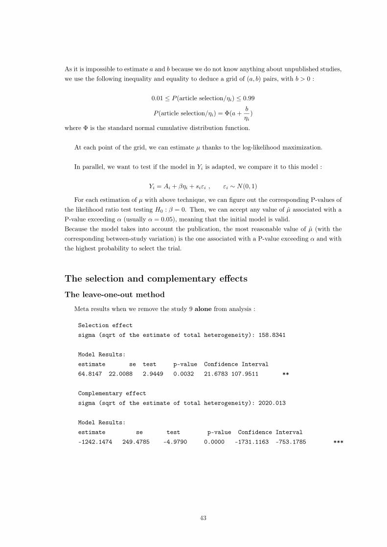
As it is impossible to estimate a and b because we do not know anything about unpublished studies,we use the following inequality and equality to deduce a grid of (a, b) pairs, with b > 0 :

0.01 ≤ P (article selection/ηi) ≤ 0.99

P (article selection/ηi) = Φ(a +b

ηi)

where Φ is the standard normal cumulative distribution function.

At each point of the grid, we can estimate µ thanks to the log-likelihood maximization.

In parallel, we want to test if the model in Yi is adapted, we compare it to this model :

Yi = Ai + βηi + siεi , εi ∼ N(0, 1)

For each estimation of µ with above technique, we can figure out the corresponding P-values ofthe likelihood ratio test testing H0 : β = 0. Then, we can accept any value of µ associated with aP-value exceeding α (usually α = 0.05), meaning that the initial model is valid.Because the model takes into account the publication, the most reasonable value of µ (with thecorresponding between-study variation) is the one associated with a P-value exceeding α and withthe highest probability to select the trial.

The selection and complementary effects

The leave-one-out method

Meta results when we remove the study 9 alone from analysis :

Selection effect

sigma (sqrt of the estimate of total heterogeneity): 158.8341

Model Results:

estimate se test p-value Confidence Interval

64.8147 22.0088 2.9449 0.0032 21.6783 107.9511 **

Complementary effect

sigma (sqrt of the estimate of total heterogeneity): 2020.013

Model Results:

estimate se test p-value Confidence Interval

-1242.1474 249.4785 -4.9790 0.0000 -1731.1163 -753.1785 ***

43

Meta analysis : Third approach

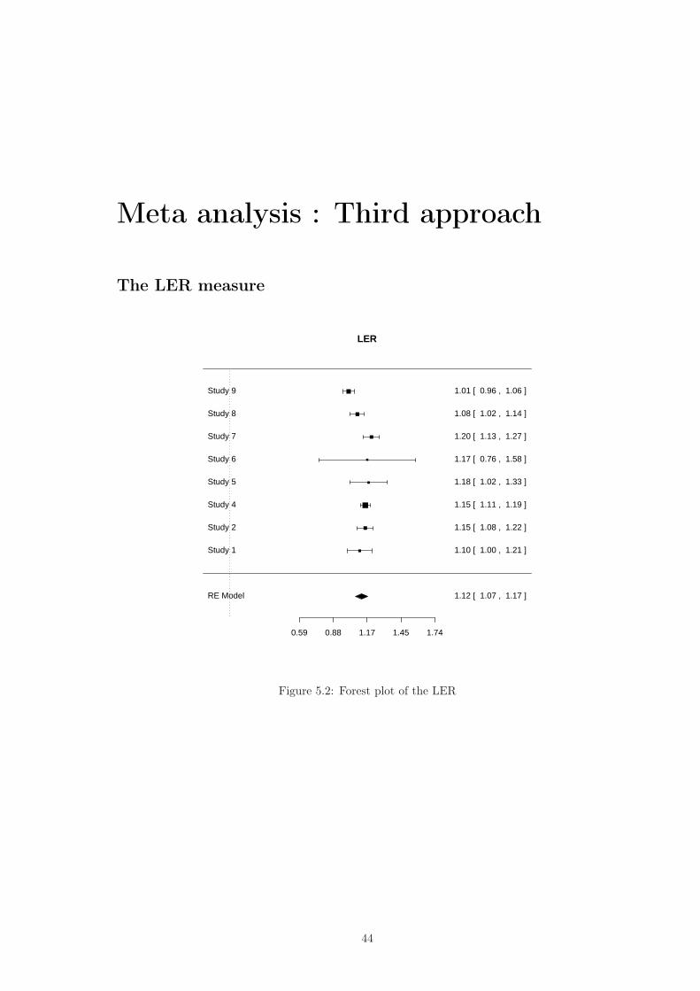
The LER measure

LER

1.12 [ 1.07 , 1.17 ]RE Model

0.59 0.88 1.17 1.45 1.74

Study 1

Study 2

Study 4

Study 5

Study 6

Study 7

Study 8

Study 9

1.10 [ 1.00 , 1.21 ]

1.15 [ 1.08 , 1.22 ]

1.15 [ 1.11 , 1.19 ]

1.18 [ 1.02 , 1.33 ]

1.17 [ 0.76 , 1.58 ]

1.20 [ 1.13 , 1.27 ]

1.08 [ 1.02 , 1.14 ]

1.01 [ 0.96 , 1.06 ]

Figure 5.2: Forest plot of the LER

44

The double effects

Selection effect

RE Model

−1038.68 599.66

Study 1

Study 2

Study 4

Study 5

Study 6

Study 7

Study 8

Study 9

Complementary effect

RE Model

−4999.61 1924.48

Study 1

Study 2

Study 4

Study 5

Study 6

Study 7

Study 8

Study 9

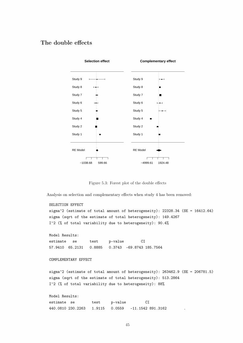
Figure 5.3: Forest plot of the double effects

Analysis on selection and complementary effects when study 4 has been removed:

SELECTION EFFECT

sigma^2 (estimate of total amount of heterogeneity): 22328.34 (SE = 16412.64)

sigma (sqrt of the estimate of total heterogeneity): 149.4267

I^2 (% of total variability due to heterogeneity): 90.4%

Model Results:

estimate se test p-value CI

57.9410 65.2131 0.8885 0.3743 -69.8743 185.7564

COMPLEMENTARY EFFECT

sigma^2 (estimate of total amount of heterogeneity): 263462.9 (SE = 206781.5)

sigma (sqrt of the estimate of total heterogeneity): 513.2864

I^2 (% of total variability due to heterogeneity): 88%

Model Results:

estimate se test p-value CI

440.0810 230.2263 1.9115 0.0559 -11.1542 891.3162 .

45

Bibliography

[1] P. Sullivan : Intercropping Principles and Production Practices, Guide, ATTRA, 2003.

[2] M.K. Andersen : Competition and complementary in annual intercrops - The role of plantavailable nutrients, Thesis, Department of Agricultural Sciences, Copenhagen, 2005.

[3] S-L.T. Normand : Tutorial in Biostatistics Meta-Analysis : Formuling, eveluating, combining,and reporting, Tutorial, Statistics in Medicine, 1999.

[4] G.R. Mohsenabadi, M.R. Jahansooz : Evalustion of Barley-Vetch intercrop at different nitro-gen rates, Article, Journal of Agricultural Sciences and Technologies, 2008.

[5] G. Agegnehu, A. Ghizaw : Yield performance and land-use effeiciency of barley and faba beanmixed cropping in Ethiopian highlands , Article, ScienceDirect, 2006.

[6] A. Gunes, A. Inal : Mineral nutrition of wheat, chickpea and lentil as affected by mixed croppingand soil moisture, Article, 2007.

[7] A. Neumann, K. Schmidtke, R. Rauber : Effects of crop density and tillage system on grainyield and N uptake from soil and atmosphere of sole and intercropped pea and oat, Article,ScienceDirect, 2005.

[8] Y.N. Song, F.S. Zhang : Effects of intercropping on crop yield and chemical and microbiologicalproperties in rhizosphere of wheat (Triticum aestivum L.), maize (Zea mays L.), and faba bean(Vicia faba L.), Article, 2006.

[9] B. Ghaley, H. Hauggaard-Nielsen : Intercropping of wheat and pea as influenced by nitrogenfertilization, Article, 2005.

[10] H. Hauggaard-Nielsen,B. Jørnsgaard : Grain legume_cereal intercropping: The practical ap-plication of diversity, competition and facilitation in arable and organic cropping systems,Article, Journal of Agricultural Science, 2004.

[11] E. Steen Jensen : Grain yield, symbiotic N2 fixation and interspecific competition for inorganicN in pea-barley intercrops, Article, 1996.

[12] J. Helenius, K. Jokinen : Yield advantage and competition in intercropped oats (Avena sativaL.) and faba bean (Viciafaba L.): Application of the hyperbolic yield-density model , Article,Field Crops Research, 1994.

[13] R. Rauber, K. Schmidtke, H. Kimpel-Freund : Konkurrenz und Ertragsvorteile in Gemengenaus Erbsen (Pisum sativum L.) und Hafer (Avena sativa L.), Article, Journal of Agronomyand Crop Science, 1999.

46

[14] M. Loreau, A. Hector : Partitioning selection and complementary in biodiversity experiments,Article, letters to nature, 2001.

[15] A. Harville : Maximum Likelihood Approaches to Variance componant Estimation and toRelated Problems, Article, Journal of the American Statistical Association, 1977.

[16] S. Duval, R. Tweedie : Trim and Fill : A simple Funnel-Plot- Based Method of Testing andAdjusting for Publication Bias in Meta-analysis, Article, Biometrics, 2000.

[17] JB. Copas, JQ. Shi : A sensitivity analysis for publication bias in systematic reviews, Article,Statistical Methods in Medical Research, 2001.

47