CHE Research Paper 68 - york.ac.uk

Truly Inefficient or Providing Better Qualityof Care? Analysing the Relationship

Between Risk-Adjusted Hospital Costs andPatients’ Health Outcomes

CHE Research Paper 68

Truly inefficient or providing better quality ofcare? Analysing the relationship between risk-adjusted hospital costs and patients’ healthoutcomes

1Nils Gutacker1Chris Bojke1Silvio Daidone2Nancy Devlin3David Parkin1Andrew Street

1Centre for Health Economics, University of York, UK2Office for Health Economics, London, UK3 NHS South East Cost, Horley, UK

October 2011

Background to series

CHE Discussion Papers (DPs) began publication in 1983 as a means of making currentresearch material more widely available to health economists and other potential users. So asto speed up the dissemination process, papers were originally published by CHE anddistributed by post to a worldwide readership.

The CHE Research Paper series takes over that function and provides access to currentresearch output via web-based publication, although hard copy will continue to be available(but subject to charge).

Acknowledgements

We would like to thank David Nuttall, Steve Morris and participants of the HESG Summer2011 conference for their inputs and comments. The project was funded by the Department ofHealth in England as part of a programme of policy research. The views expressed are thoseof the authors and may not reflect those of the funder.

Disclaimer

Papers published in the CHE Research Paper (RP) series are intended as a contribution tocurrent research. Work and ideas reported in RPs may not always represent the final positionand as such may sometimes need to be treated as work in progress. The material and viewsexpressed in RPs are solely those of the authors and should not be interpreted asrepresenting the collective views of CHE research staff or their research funders.

Further copies

Copies of this paper are freely available to download from the CHE websitewww.york.ac.uk/che/publications/ Access to downloaded material is provided on theunderstanding that it is intended for personal use. Copies of downloaded papers may bedistributed to third-parties subject to the proviso that the CHE publication source is properlyacknowledged and that such distribution is not subject to any payment.

Printed copies are available on request at a charge of £5.00 per copy. Please contact theCHE Publications Office, email [email protected], telephone 01904 321458 for furtherdetails.

Centre for Health EconomicsAlcuin CollegeUniversity of YorkYork, UKwww.york.ac.uk/che

© Nils Gutacker, Chris Bojke, Silvio Daidone, Nancy Devlin, David Parkin, Andrew Street

Truly inefficient or providing better quality of care? i

Abstract

Accounting for variation in the quality of care is a major challenge for the assessment of hospital costperformance. Because data on patients’ health improvement are generally not available, existingstudies have resorted to inherently incomplete outcome measures such as mortality or re-admissionrates. This opens up the possibility that providers of high quality care are falsely deemed inefficientand vice versa.

This study makes use of a novel dataset of routinely collected patient-reported outcomes measures(PROMs) to i) assess the degree to which cost variation is associated with variation in patients’ healthgain and ii) explore how far judgement about hospital cost performance changes when healthoutcomes are accounted for. We use multilevel modelling to address the clustering of patients inproviders and isolate unexplained cost variation.

Our results provide some evidence of a U-shaped relationship between risk-adjusted costs andoutcomes for hip replacement surgery. For the other three investigated procedures, the estimatedrelationship is sensitive to the choice of PROM instrument. We do not observe substantial changes inestimates of cost performance when outcomes are explicitly accounted for.

Keywords: hospital costs, efficiency, patient outcomes, PROMs, cost-quality relationship

ii CHE Research paper 68

Truly inefficient or providing better quality of care? 1

1. Introduction

Any health system that aims to make the best use of its scarce resources will be concerned aboutvariations in costs between different providers of the same health care. If providers can reduce coststo the level of best practice, resources might be released to provide benefits elsewhere. But inanalysing variations in provision, it is important to ensure that an assessment of best practice includesnot just costs but also patient outcomes. High costs are not always simply due to inefficiency and maybe associated with better outcomes. Low costs may sometimes be a symptom of low quality careleading to poor outcomes.

Comparative cost analysis in a multiple regression framework can help to address the question of‘which variation in cost is justifiable’ (Keeler, 1990). By benchmarking providers against each other onthe basis of their observed costs, a regulator can gain insights into the cost structure and identify theresource implications of heterogeneity (Shleifer, 1985). Over the past three decades, several hundredstudies have conducted comparative analyses of hospital costs (Hollingsworth, 2008). While thesehave contributed to a better understanding of provider heterogeneity with respect to patient case-mixand production constraints, they have not convincingly addressed the issue of variations in qualityand, particularly, health outcome as a potential explanation for observed costs (Newhouse, 1994,Jacobs et al., 2006). As a consequence, high quality hospitals may be incorrectly deemed inefficientand vice versa.

Since April 2009, all providers of publicly-funded care in the English National Health Service (NHS)are required to collect patient-reported outcome measures (PROMs) for four elective procedures:unilateral hip and knee replacements, varicose vein surgery, and groin hernia repairs (Department ofHealth, 2008a). Standardised questionnaires, including both generic (the EQ-5D) and condition-specific instruments, are collected from all eligible inpatients before and 3 or 6 months after surgery.

Building on this initiative, this paper has two aims. First, we wish to explore to what extent variation inhealth outcomes are associated with observed cost variation in the provision of care that remainsafter controlling for case-mix and production constraints. Second, we investigate whether the newinformation on health outcomes changes our judgement of provider cost performance. We performsensitivity analysis to assess the degree to which our findings depend on the choice of PROMinstrument.

Our empirical approach is to estimate multilevel models that recognise the clustering of patients withinproviders. We use these repeated observations of the hospital’s production process to distinguishrandom noise from systematic cost variation attributable to effort for which the provider can be madeaccountable. This approach differs from those typically employed in hospital efficiency studies in thatit does not require us to specify a production possibility frontier; a task that has been frequentlycriticised in the past for its distributional assumptions and its sensitivity to modelling choices(Newhouse, 1994, Skinner, 1994). Furthermore, by focussing on single production lines withhomogeneous products (e.g. hip replacement surgery) our analysis is less likely to violate theunderlying assumption of a common production function across providers (Harper et al., 2001). Ourpatient-level data also allow us to control for case-mix more thoroughly than otherwise possible inclassical single-level regression models.

2 CHE Research paper 68

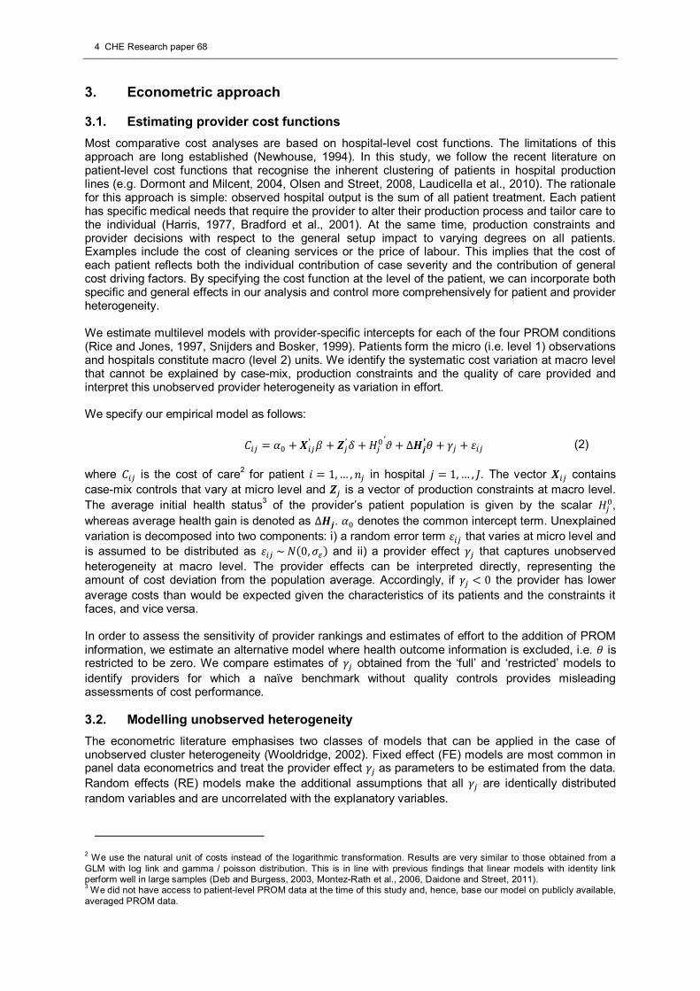
2. Conceptual framework

Social systems are often sufficiently complex to require a less-informed principal to delegate a task toa specialised agent in return for some reward

1. The principal’s objective is to ensure the publicly-

funded services are of adequate quality and delivered in a technically efficient manner. The potentialagency problems arising in such situations are well known (Lafonte and Tirole, 1993) and occur whenprincipal and agent have different objectives or value them differently and the agent’s effort isunobserved. These information asymmetries allow agents to misreport effort and pursue their ownobjectives.

One way of mitigating the problem of misreporting is to improve the information base by undertakingcomparative cost analysis. The problem is that when agents are heterogeneous with respect to theirproducts and production processes, simple comparison does not suffice. Indeed, one would thusexpect that “variation in cost is the norm rather than the exception” (Jacobs and Dawson, 2003, p.204). Any conclusions drawn from a naïve benchmark that does not account for such exogenousfactors and product characteristics would therefore be biased and the principal risks misjudgingrelative performance.

In order to obtain unbiased estimates of the agents’ efforts, Shleifer (1985, p. 324) proposes multipleregression of costs on legitimate “characteristics that make firms differ, and correct[…] for thisheterogeneity”. The natural framework for such regression analysis is the industry cost function thatunderlies all agents’ production processes. In line with the literature on hospital costs (e.g. Street etal., 2010), we can specify the hospital cost function as

ܥ = )ܥ ݓ,ݎ,ݍܻ, , ,ܼ )݁ (1)

where Y is a vector of outputs, q is a measure of quality of care provided, r and w are price vectors forcapital and labour, Z is a vector of environmental factors that constrain the production process and eis the level of effort exerted.

One potential source of variation in production costs is provider heterogeneity with respect to rangeand mix of outputs. Hospitals do not produce one homogeneous good or service. Even within patientgroups receiving the same health care intervention, certain patients will require more attention andresources than others because they suffer from more severe conditions or differ with respect to otherfactors that determine treatment costs, e.g. age, gender or number and type of comorbidities. As aconsequence, overall output of a hospital is better described as a mixture of different outputs, each ofwhich is defined by the underlying severity of the patients. Unless patients are randomly allocated tohospitals, some providers may attract a more favourable case-mix than others and achieve similarcosts while exerting less effort. It is therefore crucial to correct for output heterogeneity in order toallow for fair comparison.

A second reason why production costs may differ across hospitals is because some providers face amore adverse production environment than others. For example, hospitals may differ in their accessto factor markets and they may pay different prices for capital and labour inputs. Some of thisvariation in input prices is arguably not within the provider’s control but determined by location or theexisting infrastructure.

Production costs may also differ across hospitals because of variations in quality of care. Hospitalsmay be able to reduce the rate of hospital acquired infections by devising efficient quarantinestrategies or improve the outcome of surgery by employing experienced surgeons. Assuming thatsuch quality initiatives are costly and their results are not readily observed by the regulator, providersmay have incentives to reduce quality below some standard and misreport the cost savings asresulting from high effort (Chalkley and Malcomson, 1998). Conversely, hospitals may claim thathigher costs are the result of better quality, not low effort. As long as the regulator cannot prove thefirst or verify the latter, any cost performance assessment will be inherently incomplete.

1Such agency relationships exist not only between institutions (e.g. regulators and hospitals) but as well within institutions (e.g.

management and medical staff) (Harris, 1977). A better understanding of variations in effort amongst health care institutions istherefore crucial for policy makers and local managers alike.


So far, the ability of comparative cost studies to account for quality variation has been limited by itsmulti-dimensional nature and the inherent difficulties of measurement. Ideally, one would like tomeasure the effect of hospital treatment on each patient’s outcome, i.e. the change in health statusinduced by health care. Existing measures of output quality focus on the negative extreme of theoutcome spectrum (e.g. mortality, re-admission, adverse events) but fail to account for improvementsin health. In contrast, PROMs allow measuring variation across the entire spectrum and can be usedto determine the production costs of health improvement.


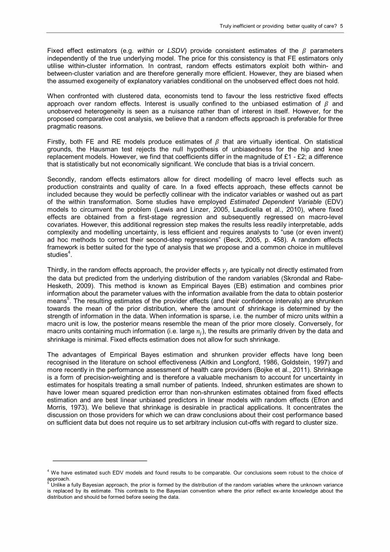
3. Econometric approach

3.1. Estimating provider cost functions

Most comparative cost analyses are based on hospital-level cost functions. The limitations of thisapproach are long established (Newhouse, 1994). In this study, we follow the recent literature onpatient-level cost functions that recognise the inherent clustering of patients in hospital productionlines (e.g. Dormont and Milcent, 2004, Olsen and Street, 2008, Laudicella et al., 2010). The rationalefor this approach is simple: observed hospital output is the sum of all patient treatment. Each patienthas specific medical needs that require the provider to alter their production process and tailor care tothe individual (Harris, 1977, Bradford et al., 2001). At the same time, production constraints andprovider decisions with respect to the general setup impact to varying degrees on all patients.Examples include the cost of cleaning services or the price of labour. This implies that the cost ofeach patient reflects both the individual contribution of case severity and the contribution of generalcost driving factors. By specifying the cost function at the level of the patient, we can incorporate bothspecific and general effects in our analysis and control more comprehensively for patient and providerheterogeneity.

We estimate multilevel models with provider-specific intercepts for each of the four PROM conditions(Rice and Jones, 1997, Snijders and Bosker, 1999). Patients form the micro (i.e. level 1) observationsand hospitals constitute macro (level 2) units. We identify the systematic cost variation at macro levelthat cannot be explained by case-mix, production constraints and the quality of care provided andinterpret this unobserved provider heterogeneity as variation in effort.

We specify our empirical model as follows:

ܥ = ߙ + ′ +ߚ

+ߜ′ ܪ′ߴ+ ∆

+ߠ′ ߛ + ߝ (2)

where ܥ is the cost of care2

for patient ݅ൌ ͳǡǥ ǡ݊ in hospital ݆ൌ ͳǡǥ ǡܬ. The vector contains

case-mix controls that vary at micro level and is a vector of production constraints at macro level.

The average initial health status3

of the provider’s patient population is given by the scalar ܪ,

whereas average health gain is denoted as ο. ߙ denotes the common intercept term. Unexplained

variation is decomposed into two components: i) a random error term ߝ that varies at micro level and

is assumed to be distributed as �̱ߝ �ܰ (Ͳǡߪఌ) and ii) a provider effect ߛ that captures unobserved

heterogeneity at macro level. The provider effects can be interpreted directly, representing theamount of cost deviation from the population average. Accordingly, if ߛ < 0 the provider has lower

average costs than would be expected given the characteristics of its patients and the constraints itfaces, and vice versa.

In order to assess the sensitivity of provider rankings and estimates of effort to the addition of PROMinformation, we estimate an alternative model where health outcome information is excluded, i.e. ߠ isrestricted to be zero. We compare estimates of ߛ obtained from the ‘full’ and ‘restricted’ models to

identify providers for which a naïve benchmark without quality controls provides misleadingassessments of cost performance.

3.2. Modelling unobserved heterogeneity

The econometric literature emphasises two classes of models that can be applied in the case ofunobserved cluster heterogeneity (Wooldridge, 2002). Fixed effect (FE) models are most common inpanel data econometrics and treat the provider effect ߛ as parameters to be estimated from the data.

Random effects (RE) models make the additional assumptions that all ߛ are identically distributed

random variables and are uncorrelated with the explanatory variables.

2We use the natural unit of costs instead of the logarithmic transformation. Results are very similar to those obtained from a

GLM with log link and gamma / poisson distribution. This is in line with previous findings that linear models with identity linkperform well in large samples (Deb and Burgess, 2003, Montez-Rath et al., 2006, Daidone and Street, 2011).3

We did not have access to patient-level PROM data at the time of this study and, hence, base our model on publicly available,averaged PROM data.


Fixed effect estimators (e.g. within or LSDV) provide consistent estimates of the ߚ parametersindependently of the true underlying model. The price for this consistency is that FE estimators onlyutilise within-cluster information. In contrast, random effects estimators exploit both within- andbetween-cluster variation and are therefore generally more efficient. However, they are biased whenthe assumed exogeneity of explanatory variables conditional on the unobserved effect does not hold.

When confronted with clustered data, economists tend to favour the less restrictive fixed effectsapproach over random effects. Interest is usually confined to the unbiased estimation of ߚ andunobserved heterogeneity is seen as a nuisance rather than of interest in itself. However, for theproposed comparative cost analysis, we believe that a random effects approach is preferable for threepragmatic reasons.

Firstly, both FE and RE models produce estimates of ߚ that are virtually identical. On statisticalgrounds, the Hausman test rejects the null hypothesis of unbiasedness for the hip and kneereplacement models. However, we find that coefficients differ in the magnitude of £1 - £2; a differencethat is statistically but not economically significant. We conclude that bias is a trivial concern.

Secondly, random effects estimators allow for direct modelling of macro level effects such asproduction constraints and quality of care. In a fixed effects approach, these effects cannot beincluded because they would be perfectly collinear with the indicator variables or washed out as partof the within transformation. Some studies have employed Estimated Dependent Variable (EDV)models to circumvent the problem (Lewis and Linzer, 2005, Laudicella et al., 2010), where fixedeffects are obtained from a first-stage regression and subsequently regressed on macro-levelcovariates. However, this additional regression step makes the results less readily interpretable, addscomplexity and modelling uncertainty, is less efficient and requires analysts to “use (or even invent)ad hoc methods to correct their second-step regressions” (Beck, 2005, p. 458). A random effectsframework is better suited for the type of analysis that we propose and a common choice in multilevelstudies

4.

Thirdly, in the random effects approach, the provider effects ߛ are typically not directly estimated from

the data but predicted from the underlying distribution of the random variables (Skrondal and Rabe-Hesketh, 2009). This method is known as Empirical Bayes (EB) estimation and combines priorinformation about the parameter values with the information available from the data to obtain posteriormeans

5. The resulting estimates of the provider effects (and their confidence intervals) are shrunken

towards the mean of the prior distribution, where the amount of shrinkage is determined by thestrength of information in the data. When information is sparse, i.e. the number of micro units within amacro unit is low, the posterior means resemble the mean of the prior more closely. Conversely, formacro units containing much information (i.e. large ݊), the results are primarily driven by the data and

shrinkage is minimal. Fixed effects estimation does not allow for such shrinkage.

The advantages of Empirical Bayes estimation and shrunken provider effects have long beenrecognised in the literature on school effectiveness (Aitkin and Longford, 1986, Goldstein, 1997) andmore recently in the performance assessment of health care providers (Bojke et al., 2011). Shrinkageis a form of precision-weighting and is therefore a valuable mechanism to account for uncertainty inestimates for hospitals treating a small number of patients. Indeed, shrunken estimates are shown tohave lower mean squared prediction error than non-shrunken estimates obtained from fixed effectsestimation and are best linear unbiased predictors in linear models with random effects (Efron andMorris, 1973). We believe that shrinkage is desirable in practical applications. It concentrates thediscussion on those providers for which we can draw conclusions about their cost performance basedon sufficient data but does not require us to set arbitrary inclusion cut-offs with regard to cluster size.

4We have estimated such EDV models and found results to be comparable. Our conclusions seem robust to the choice of

approach.5

Unlike a fully Bayesian approach, the prior is formed by the distribution of the random variables where the unknown varianceis replaced by its estimate. This contrasts to the Bayesian convention where the prior reflect ex-ante knowledge about thedistribution and should be formed before seeing the data.


4. Data

4.1. Hospital Episode Statistics

Our study uses patient level data extracted from the Hospital Episode Statistics database (HES) forthe financial year 2009/10. HES contains detailed information about care provided to all patientstreated in NHS hospitals. The unit of observations in HES is the episode of care under the supervisionof one consultant (“finished consultant episode” (FCE)). In order to obtain the full level of patientinformation documented across the inpatient stay, we link all associated FCEs and create providerspells (Castelli et al., 2008). We select only those spells in which eligible PROM procedures havebeen performed (see NHS Information Centre (2010, pp. 22-28) for inclusion criteria). Further, werestrict our analysis to NHS providers due to the poor quality of data submitted by the independentsector (Mason et al., 2010).

All patients are allocated to a Healthcare Resource Group (HRG v.4). By design, HRGs are expectedto explain a substantial amount of variation in observed costs. The grouping algorithm used by theNHS Information Centre (NHS IC) assigns HRGs to each FCE. We extract information on the HRG ofthe episode in which the (first) relevant PROM procedure has taken place and construct indicatorvariables for the ten most frequent HRGs. All other observations are grouped in the category ‘OtherHRG’. The most frequent HRG is set as base category in the regressions.

The construction of any classification system necessarily requires a trade-off between parsimony andhomogeneity of the resulting groups. As a consequence, HRGs are unlikely to capture all variationacross providers. Hence, we include a set of variables that are based on diagnostic codes (ICD-10)and procedure codes (OPCS-4.5). These include the main reason and type of surgery (PROM-specific), whether it was a primary or revision surgery, and the weighted Charlson index as a measureof co-morbidity (Charlson et al., 1987). Further, we generate counts of non-duplicate, secondarydiagnoses and procedure codes within a spell as further controls for co-morbidities and complications.

We account for patient demographics by sorting patients into age quintiles and create an indicatorvariable for male gender. To characterise the inpatient stay itself, we construct indicator variables fortransfers in and out of hospital, whether the patient is discharged home or not, multi-episode spellsand in-hospital mortality.

We construct variables that capture the influence of observed characteristics of the provider andproduction environment that are likely to constrain the production process. Larger providers may beable to realise economies of scale and we generate a measure of size based on the count of patientstreated by the provider. To address economies of scope, we create an index of specialisation thatreflects the dispersion of HRGs treated within the hospital (Daidone and D’Amico, 2009). The indexresembles a Gini index and is bound between zero (no specialisation) and one (all patients of hospitalj fall into one HRG). Finally, hospital trusts are categorised into teaching and non-teaching facilitiesbased on the classification system adopted by the National Patient Safety Agency (2009).

4.2. Reference cost

Hospital Episode Statistics do not include information on the cost of care. However, NHS trusts arerequired to provide information on their costs to the Department of Health for the annual compilationof the reference cost schedule and calculation of reimbursement prices. We utilise the 2009/10 returnto construct patient-level cost data.

The reference cost report is implemented using a top-down costing methodology. Here, total hospitalcosts are progressively cascaded down through a hierarchy of costing levels, starting at treatmentservices, to specialities and finally to individual HRGs. Costs at HRG-level are reported separately fordepartments and are further disaggregated according to admission type (day case, elective andemergency care) and length of stay, where HRG-specific trim points are used to differentiate betweenshort, average and long inpatient spells. We map the reference cost to our sample according to thealgorithm documented in Laudicella et al (2010). In absence of an agreed methodology on how toaggregate cost from FCE to spell level (Daidone and Street, 2011), we assign the cost of the FCE inwhich the (first) PROM procedure has taken place.


We adjust patient costs by the Market Forces Factor (MFF) specific to the provider. The MFF is anindex of relative prices for buildings, land and labour that is used by the English Department of Healthto adjust reimbursement for what is deemed unavoidable variation in input prices (Department ofHealth, 2008b). By applying this index to the costs reported in the reference cost schedule, we canwash out justifiable variation in input prices directly.

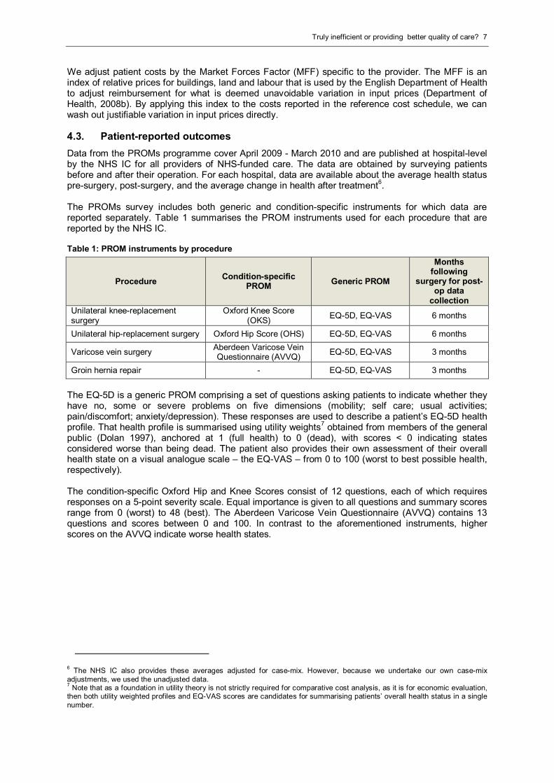
4.3. Patient-reported outcomes

Data from the PROMs programme cover April 2009 - March 2010 and are published at hospital-levelby the NHS IC for all providers of NHS-funded care. The data are obtained by surveying patientsbefore and after their operation. For each hospital, data are available about the average health statuspre-surgery, post-surgery, and the average change in health after treatment

6.

The PROMs survey includes both generic and condition-specific instruments for which data arereported separately. Table 1 summarises the PROM instruments used for each procedure that arereported by the NHS IC.

Table 1: PROM instruments by procedure

ProcedureCondition-specific

PROMGeneric PROM

Monthsfollowing

surgery for post-op data

collectionUnilateral knee-replacementsurgery

Oxford Knee Score(OKS)

EQ-5D, EQ-VAS 6 months

Unilateral hip-replacement surgery Oxford Hip Score (OHS) EQ-5D, EQ-VAS 6 months

Varicose vein surgeryAberdeen Varicose VeinQuestionnaire (AVVQ)

EQ-5D, EQ-VAS 3 months

Groin hernia repair - EQ-5D, EQ-VAS 3 months

The EQ-5D is a generic PROM comprising a set of questions asking patients to indicate whether theyhave no, some or severe problems on five dimensions (mobility; self care; usual activities;pain/discomfort; anxiety/depression). These responses are used to describe a patient’s EQ-5D healthprofile. That health profile is summarised using utility weights

7obtained from members of the general

public (Dolan 1997), anchored at 1 (full health) to 0 (dead), with scores < 0 indicating statesconsidered worse than being dead. The patient also provides their own assessment of their overallhealth state on a visual analogue scale – the EQ-VAS – from 0 to 100 (worst to best possible health,respectively).

The condition-specific Oxford Hip and Knee Scores consist of 12 questions, each of which requiresresponses on a 5-point severity scale. Equal importance is given to all questions and summary scoresrange from 0 (worst) to 48 (best). The Aberdeen Varicose Vein Questionnaire (AVVQ) contains 13questions and scores between 0 and 100. In contrast to the aforementioned instruments, higherscores on the AVVQ indicate worse health states.

6The NHS IC also provides these averages adjusted for case-mix. However, because we undertake our own case-mix

adjustments, we used the unadjusted data.7

Note that as a foundation in utility theory is not strictly required for comparative cost analysis, as it is for economic evaluation,then both utility weighted profiles and EQ-VAS scores are candidates for summarising patients’ overall health status in a singlenumber.


5. Results

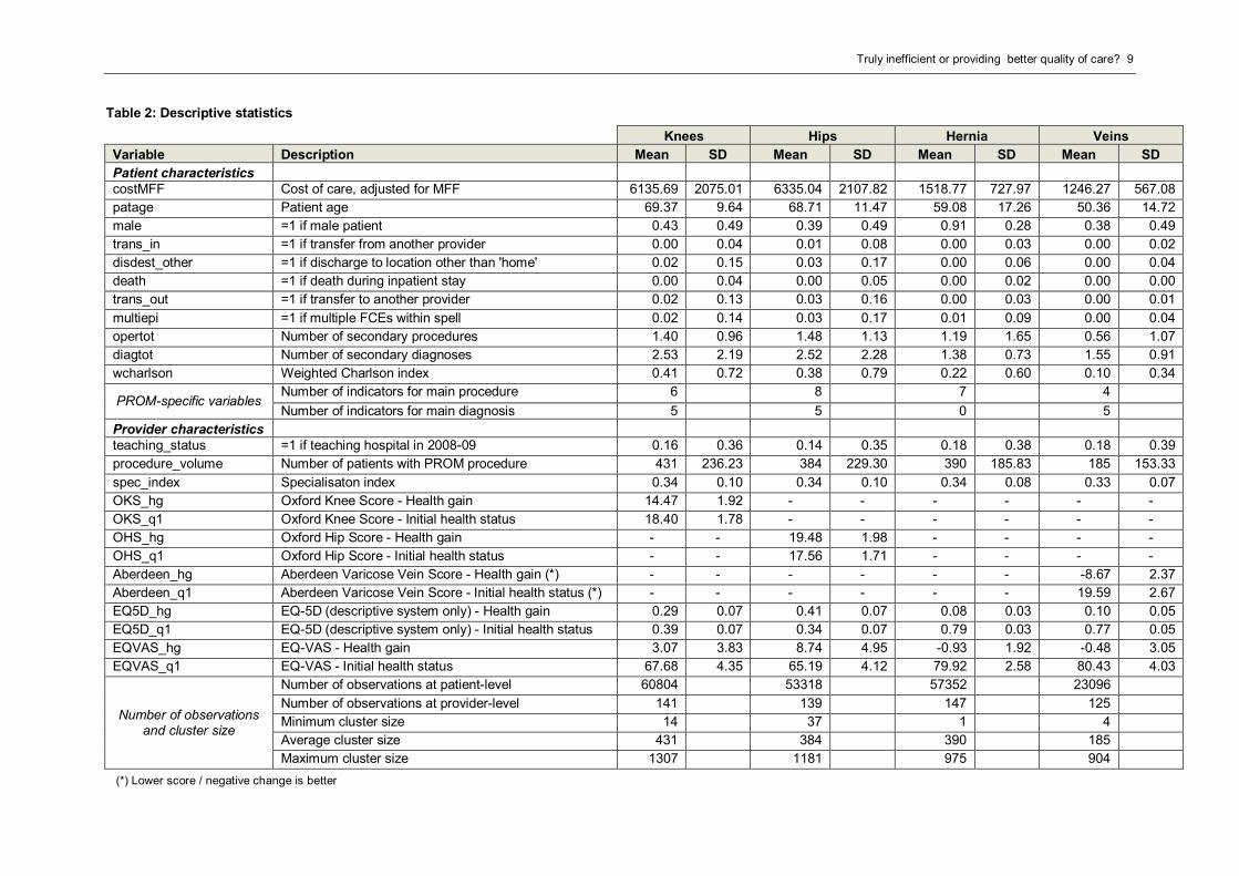
5.1. Descriptive statistics

We present descriptive statistics in Table 2.

Each of the four conditions is sufficiently populated to allow for precise estimation of case-mix effectsat patient level. In contrast, the number of providers is comparably low (125 to 147 hospitals),reinforcing the value of multilevel analysis as compared to traditional hospital-level analysis.Furthermore, we observe large variations in cluster size within and across production lines. Onewould thus expect that provider effects are estimated with varying degrees of precision and thatshrinkage can contribute to a more conservative assessment of hospitals’ efforts.

The cost of care varies considerably across providers for each of the four procedures. For example,for knee replacement surgery we observe average costs of care by provider that range from below£2,000 to more than £10,000. High cost cases are not confined to one or two providers. Rather, weobserve that many hospitals report costs for patients in excess of two standard deviations above thenational average. This suggests that these cases are truly high-cost cases and not artefacts of theway local accounting system operate or how costs are assigned to patients. We therefore retain allobservations in our sample and do not trim ‘outliers’ based on observed costs.

The generic nature of EQ-5D and EQ-VAS allows for comparison of health outcomes acrossconditions. Patients undergoing hip or knee replacement surgery experience substantially largerincreases in health status than those receiving groin hernia or varicose vein surgery. This isconsistent with the less serious nature of the underlying conditions. We observe disagreementbetween EQ-5D and EQ-VAS on the direction of health change for the latter groups of patients.Whether this is a result of aggregation or a genuine difference between instruments cannot beexplored with our dataset.

5.2. Regression results

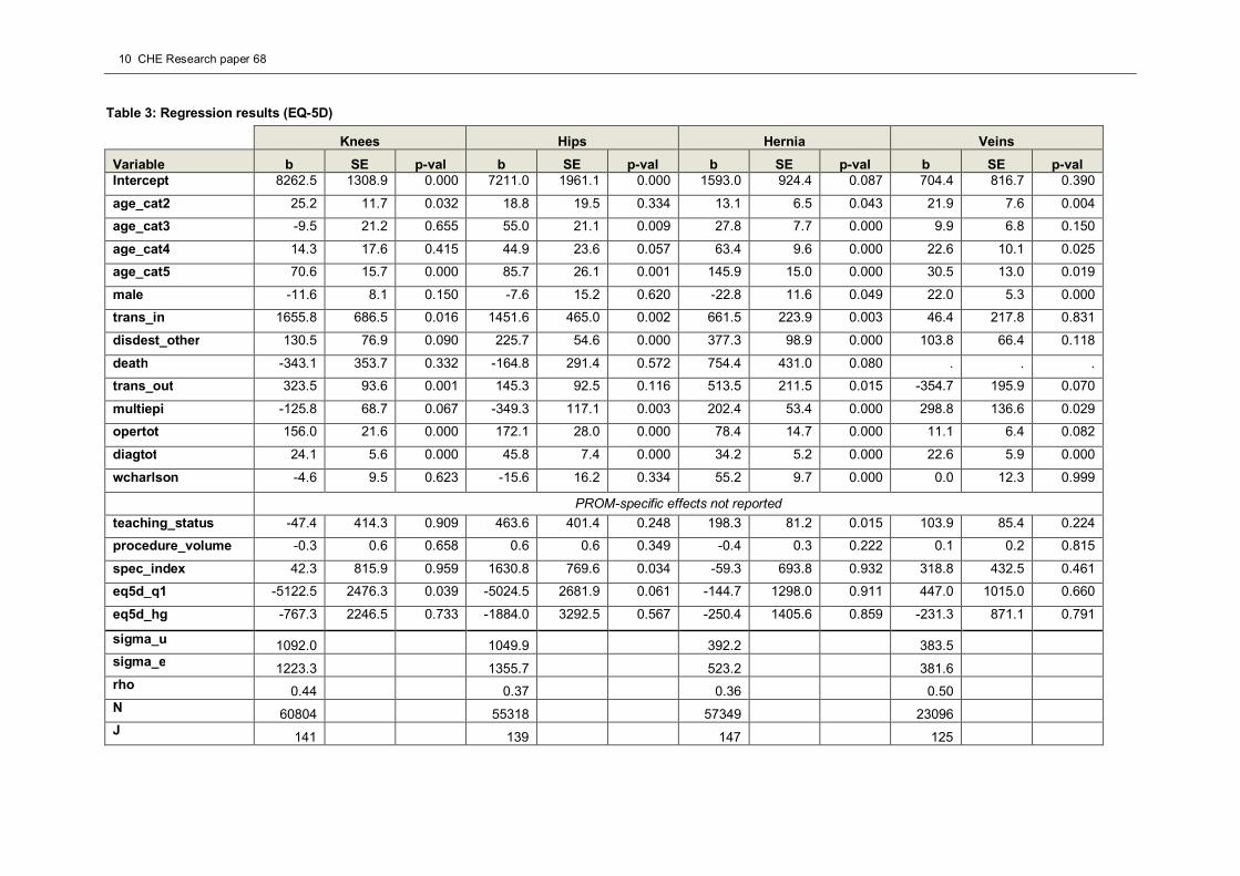
5.2.1. Baseline estimates

Table 3 presents regression results from a model with EQ-5D outcome information. The reportedstandard errors are robust to heteroscedasticity.

We find significant coefficients on the majority of HRG variables (not reported). This indicates that thecurrent reimbursement system is able to distinguish between different types of patients and theirexpected costs. Several other patient characteristics explain costs over and above the allocated HRG.For example, we observe an age effect and find that certain types of main diagnoses and proceduresare significant predictors of treatment costs. Costs are higher for patients that undergo moreprocedures or suffer from a higher number of comorbidities as well as for patients that are transferredin or out of hospital or not discharged to their usual place of residence.

The results at provider-level are less clear cut. The average cost of patients treated in teachinghospitals is generally higher than in non-teaching hospitals but the effect is statistically significant onlyfor groin hernia repair. We do not find conclusive evidence that NHS hospitals realise positiveeconomies of scale or scope within production lines. This is somewhat surprising given the substantialdifferences in volume and, to a lesser degree, specialisation observed across providers for each ofthe four conditions.

With respect to PROM data, we find that the coefficient on initial health status shows the expectednegative sign for three out of four conditions but is only statistically significant for the two orthopaedicprocedures. Patients that present with higher health status at admission require fewer resources thanpatients in worse conditions; a result that seems intuitively correct. The relationship between healthgain and costs is negative in all four models. This would indicate that some providers are able tosecure greater health gains and provide care at lower cost than other providers. However, no resultsare statistically significant at the 5% confidence level.


Table 2: Descriptive statistics

Knees Hips Hernia Veins

Variable Description Mean SD Mean SD Mean SD Mean SD

Patient characteristicscostMFF Cost of care, adjusted for MFF 6135.69 2075.01 6335.04 2107.82 1518.77 727.97 1246.27 567.08

patage Patient age 69.37 9.64 68.71 11.47 59.08 17.26 50.36 14.72

male =1 if male patient 0.43 0.49 0.39 0.49 0.91 0.28 0.38 0.49

trans_in =1 if transfer from another provider 0.00 0.04 0.01 0.08 0.00 0.03 0.00 0.02

disdest_other =1 if discharge to location other than 'home' 0.02 0.15 0.03 0.17 0.00 0.06 0.00 0.04

death =1 if death during inpatient stay 0.00 0.04 0.00 0.05 0.00 0.02 0.00 0.00

trans_out =1 if transfer to another provider 0.02 0.13 0.03 0.16 0.00 0.03 0.00 0.01

multiepi =1 if multiple FCEs within spell 0.02 0.14 0.03 0.17 0.01 0.09 0.00 0.04

opertot Number of secondary procedures 1.40 0.96 1.48 1.13 1.19 1.65 0.56 1.07

diagtot Number of secondary diagnoses 2.53 2.19 2.52 2.28 1.38 0.73 1.55 0.91

wcharlson Weighted Charlson index 0.41 0.72 0.38 0.79 0.22 0.60 0.10 0.34

PROM-specific variablesNumber of indicators for main procedure 6 8 7 4

Number of indicators for main diagnosis 5 5 0 5

Provider characteristicsteaching_status =1 if teaching hospital in 2008-09 0.16 0.36 0.14 0.35 0.18 0.38 0.18 0.39

procedure_volume Number of patients with PROM procedure 431 236.23 384 229.30 390 185.83 185 153.33

spec_index Specialisaton index 0.34 0.10 0.34 0.10 0.34 0.08 0.33 0.07

OKS_hg Oxford Knee Score - Health gain 14.47 1.92 - - - - - -

OKS_q1 Oxford Knee Score - Initial health status 18.40 1.78 - - - - - -

OHS_hg Oxford Hip Score - Health gain - - 19.48 1.98 - - - -

OHS_q1 Oxford Hip Score - Initial health status - - 17.56 1.71 - - - -

Aberdeen_hg Aberdeen Varicose Vein Score - Health gain (*) - - - - - - -8.67 2.37

Aberdeen_q1 Aberdeen Varicose Vein Score - Initial health status (*) - - - - - - 19.59 2.67

EQ5D_hg EQ-5D (descriptive system only) - Health gain 0.29 0.07 0.41 0.07 0.08 0.03 0.10 0.05

EQ5D_q1 EQ-5D (descriptive system only) - Initial health status 0.39 0.07 0.34 0.07 0.79 0.03 0.77 0.05

EQVAS_hg EQ-VAS - Health gain 3.07 3.83 8.74 4.95 -0.93 1.92 -0.48 3.05

EQVAS_q1 EQ-VAS - Initial health status 67.68 4.35 65.19 4.12 79.92 2.58 80.43 4.03

Number of observationsand cluster size

Number of observations at patient-level 60804 53318 57352 23096

Number of observations at provider-level 141 139 147 125

Minimum cluster size 14 37 1 4

Average cluster size 431 384 390 185

Maximum cluster size 1307 1181 975 904

(*) Lower score / negative change is better


Table 3: Regression results (EQ-5D)


Variable b SE p-val b SE p-val b SE p-val b SE p-valIntercept 8262.5 1308.9 0.000 7211.0 1961.1 0.000 1593.0 924.4 0.087 704.4 816.7 0.390

age_cat2 25.2 11.7 0.032 18.8 19.5 0.334 13.1 6.5 0.043 21.9 7.6 0.004

age_cat3 -9.5 21.2 0.655 55.0 21.1 0.009 27.8 7.7 0.000 9.9 6.8 0.150

age_cat4 14.3 17.6 0.415 44.9 23.6 0.057 63.4 9.6 0.000 22.6 10.1 0.025

age_cat5 70.6 15.7 0.000 85.7 26.1 0.001 145.9 15.0 0.000 30.5 13.0 0.019

male -11.6 8.1 0.150 -7.6 15.2 0.620 -22.8 11.6 0.049 22.0 5.3 0.000

trans_in 1655.8 686.5 0.016 1451.6 465.0 0.002 661.5 223.9 0.003 46.4 217.8 0.831

disdest_other 130.5 76.9 0.090 225.7 54.6 0.000 377.3 98.9 0.000 103.8 66.4 0.118

death -343.1 353.7 0.332 -164.8 291.4 0.572 754.4 431.0 0.080 . . .

trans_out 323.5 93.6 0.001 145.3 92.5 0.116 513.5 211.5 0.015 -354.7 195.9 0.070

multiepi -125.8 68.7 0.067 -349.3 117.1 0.003 202.4 53.4 0.000 298.8 136.6 0.029

opertot 156.0 21.6 0.000 172.1 28.0 0.000 78.4 14.7 0.000 11.1 6.4 0.082

diagtot 24.1 5.6 0.000 45.8 7.4 0.000 34.2 5.2 0.000 22.6 5.9 0.000

wcharlson -4.6 9.5 0.623 -15.6 16.2 0.334 55.2 9.7 0.000 0.0 12.3 0.999

PROM-specific effects not reported

teaching_status -47.4 414.3 0.909 463.6 401.4 0.248 198.3 81.2 0.015 103.9 85.4 0.224

procedure_volume -0.3 0.6 0.658 0.6 0.6 0.349 -0.4 0.3 0.222 0.1 0.2 0.815

spec_index 42.3 815.9 0.959 1630.8 769.6 0.034 -59.3 693.8 0.932 318.8 432.5 0.461

eq5d_q1 -5122.5 2476.3 0.039 -5024.5 2681.9 0.061 -144.7 1298.0 0.911 447.0 1015.0 0.660

eq5d_hg -767.3 2246.5 0.733 -1884.0 3292.5 0.567 -250.4 1405.6 0.859 -231.3 871.1 0.791

sigma_u1092.0 1049.9 392.2 383.5

sigma_e1223.3 1355.7 523.2 381.6

rho 0.44 0.37 0.36 0.50N 60804 55318 57349 23096J

141 139 147 125


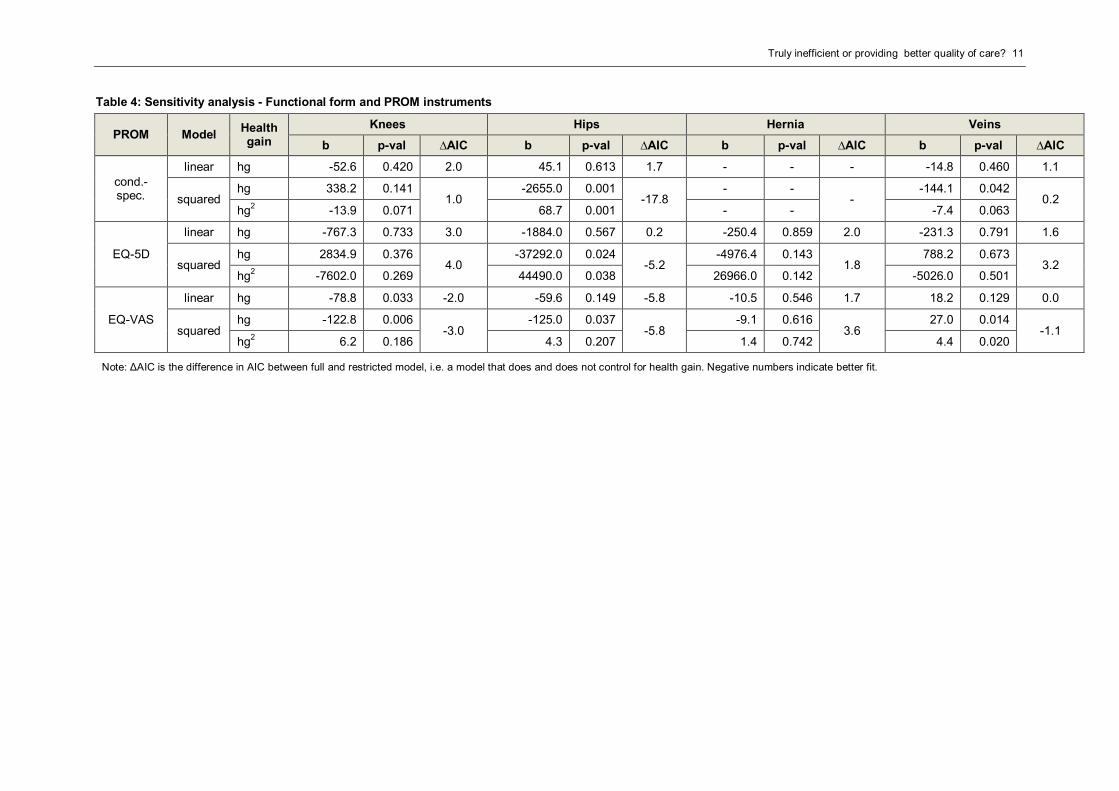
Table 4: Sensitivity analysis - Functional form and PROM instruments

PROM ModelHealthgain


b p-val ∆AIC b p-val ∆AIC b p-val ∆AIC b p-val ∆AIC

cond.-spec.

linear hg -52.6 0.420 2.0 45.1 0.613 1.7 - - - -14.8 0.460 1.1

squaredhg 338.2 0.141

1.0-2655.0 0.001

-17.8- -

--144.1 0.042

0.2hg2 -13.9 0.071 68.7 0.001 - - -7.4 0.063

EQ-5D

linear hg -767.3 0.733 3.0 -1884.0 0.567 0.2 -250.4 0.859 2.0 -231.3 0.791 1.6

squaredhg 2834.9 0.376

4.0-37292.0 0.024

-5.2-4976.4 0.143

1.8788.2 0.673

3.2hg2 -7602.0 0.269 44490.0 0.038 26966.0 0.142 -5026.0 0.501

EQ-VAS

linear hg -78.8 0.033 -2.0 -59.6 0.149 -5.8 -10.5 0.546 1.7 18.2 0.129 0.0

squaredhg -122.8 0.006

-3.0-125.0 0.037

-5.8-9.1 0.616

3.627.0 0.014

-1.1hg2 6.2 0.186 4.3 0.207 1.4 0.742 4.4 0.020

Note: ΔAIC is the difference in AIC between full and restricted model, i.e. a model that does and does not control for health gain. Negative numbers indicate better fit.


5.2.2. Sensitivity analysis – source of PROMs data

In order to test the stability of our findings, we scrutinise two modelling choices: First, we re-estimatethe various models using EQ-VAS and condition-specific PROMs. While there are good reasons toprefer generic instruments over condition-specific instruments, for example because the formerfacilitates broader comparisons across disease areas, one should not a priori exclude the latter forthis type of analysis. Second, we test for a parabolic relationship between health outcome and costsas previously reported in the literature (Hvenegaard et al., online first). The Akaike Information Criteria(AIC) is used to compare the fit of the ‘full’ and ‘restricted’ model, where improvements in model fit areindicated by negative changes. Results of this sensitivity analysis are summarised in Table 4.

We find a negative linear relationship between health gain and costs for knee replacement surgerywhen outcomes are measured via EQ-VAS. The statistical significance of this specific model is re-emphasised by the improvement in AIC. However, we do not find support for this result with regard tothe other two PROM instruments nor any of the other procedures.

In contrast, we find stronger evidence of a non-linear relationship between health gain and costs forhip replacement surgery using either Oxford Hip Score or utility-weighted EQ-5D. The estimatedrelationship is U-shaped with initially negative marginal effects that turn positive when average healthgain passes a saddle point. This suggests that those providers located on the downwards sloping sideof the curve could substantially improve health outcomes while reducing costs. In contrast, providerson the upward sloping side can only achieve better outcomes by investing more resources.

For varicose vein surgery, the estimated relationship is positive and exponential for the EQ-VAS andthe Aberdeen Varicose Vein score, although the latter is only jointly statistically significant. One mayinterpret this as the right-hand side of the U-shaped relationship that we observe for hip replacementsurgery.

5.3. Impact on provider effects

We now turn to the assessment of providers’ efforts to contain cost. We illustrate our results with theexample of hip replacement surgery and the Oxford Hip Score.

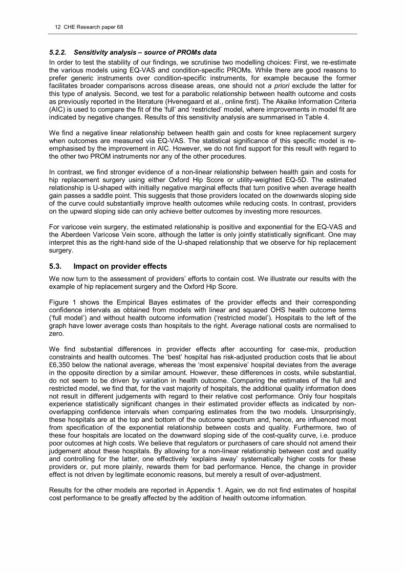
Figure 1 shows the Empirical Bayes estimates of the provider effects and their correspondingconfidence intervals as obtained from models with linear and squared OHS health outcome terms(‘full model’) and without health outcome information (‘restricted model’). Hospitals to the left of thegraph have lower average costs than hospitals to the right. Average national costs are normalised tozero.

We find substantial differences in provider effects after accounting for case-mix, productionconstraints and health outcomes. The ‘best’ hospital has risk-adjusted production costs that lie about£6,350 below the national average, whereas the ‘most expensive’ hospital deviates from the averagein the opposite direction by a similar amount. However, these differences in costs, while substantial,do not seem to be driven by variation in health outcome. Comparing the estimates of the full andrestricted model, we find that, for the vast majority of hospitals, the additional quality information doesnot result in different judgements with regard to their relative cost performance. Only four hospitalsexperience statistically significant changes in their estimated provider effects as indicated by non-overlapping confidence intervals when comparing estimates from the two models. Unsurprisingly,these hospitals are at the top and bottom of the outcome spectrum and, hence, are influenced mostfrom specification of the exponential relationship between costs and quality. Furthermore, two ofthese four hospitals are located on the downward sloping side of the cost-quality curve, i.e. producepoor outcomes at high costs. We believe that regulators or purchasers of care should not amend theirjudgement about these hospitals. By allowing for a non-linear relationship between cost and qualityand controlling for the latter, one effectively ‘explains away’ systematically higher costs for theseproviders or, put more plainly, rewards them for bad performance. Hence, the change in providereffect is not driven by legitimate economic reasons, but merely a result of over-adjustment.

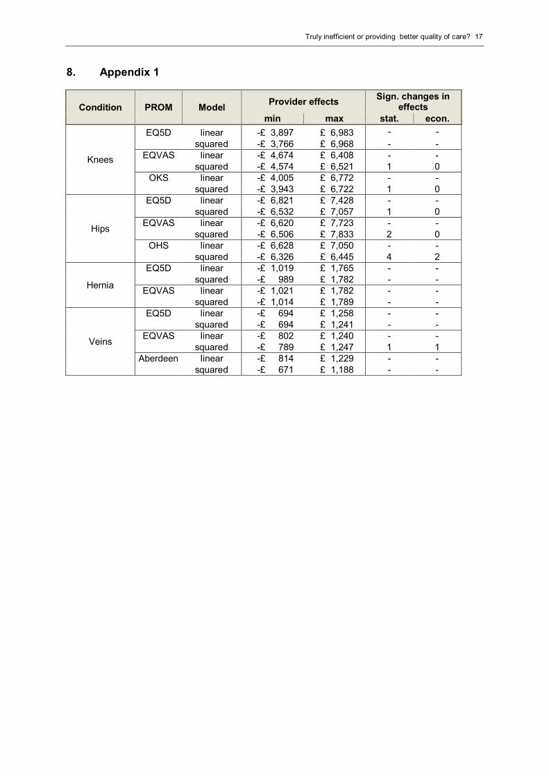
Results for the other models are reported in Appendix 1. Again, we do not find estimates of hospitalcost performance to be greatly affected by the addition of health outcome information.


Figure 1: Provider effects for hip surgery – OHS

-100

00

-500

00

500

01

00

00

Pro

vid

er

effe

ctin

GB

P

0 20 40 60 80 100 120 140139 NHS trusts

Effect - full CI - full

Effect - restricted CI - restricted


6. Discussion and conclusions

The aim of this paper is to measure cost variation in the provision of four selected surgical proceduresunder special consideration of differences in the quality of care provided. Our work builds on a newpolicy initiative by the English Department of Health to collect patient-reported health outcomes usinggeneric and condition-specific instruments. This study is a first attempt to incorporate health outcomesinto comparative cost analysis and explore whether this new measure of quality changes judgementsabout the relative performance of NHS hospitals. We make a case for multilevel modelling withprecision-weighting and highlight the advantages of this technique over other approaches toperformance measurement.

Our results suggest that systematic cost differences exist across hospitals in the provision of surgicalprocedures that is not due to either patient or production process characteristics. Some of thevariation in costs can be associated with the average health outcome and we find evidence of a non-linear relationship between cost and outcomes for hip replacement and varicose vein surgery. For ahandful of hospitals, such health outcome adjustment leads to a statistically significant improvementin their estimated cost performance. However, we have argued that the economic judgement shoulddiffer depending on whether the hospital is located on the positive or negative slope of the cost-qualitycurve and that one should be aware of the risk of over-adjustment.

Several implications for policy makers and future research arise from our results. First, the impact ofhealth outcome information on provider rankings and estimates of cost containment effort is, at best,minimal. This casts doubt on claims that might be made by some hospitals that their higher productioncosts are a consequence of investing in better care that produces better health outcomes. That said,our analysis is restricted to outcome information averaged at provider level and it will be interesting tosee whether this finding still holds for analyses that utilise patient level outcome data.

Second, our study has only explored the association between cost and health outcome, but cannotascertain causality. Future work should aim to overcome this limitation and specifically account for thepotential endogeneity.

Third, if the relationship between cost and quality is indeed non-linear, pay-for-performance andquality bonus programs have to acknowledge non-constant marginal costs and set different prices fordifferent health outcomes. If the association between outcomes and cost is negative or non-existent(see e.g. groin hernia repair) then quality bonus payments of any form should be understood asincentive payments in excess of production costs. The way in which quality incentive schemes aredesigned might therefore be quite different for different conditions and depend on the observedassociation between costs and outcomes. In some cases, a purchaser or commissioner will need toreimburse the additional costs of production in order to allow providers to break even whereas in theother cases non-financial incentives may suffice.

Fourth, at this early stage of the PROM initiative and on the basis of our preliminary analysis, wecannot single out a preferred PROM instrument that should be applied exclusively in future analysesof hospital cost performance. We therefore recommend using both generic and condition-specificinstruments and conducting sensitivity analysis with regard to the choice of PROM instrument as wehave done here.


7. References

Aitkin M, Longford N. 1986. Statistical modelling issues in school effectiveness studies. Journal of theRoyal Statistical Society. Series A (General), 149, 1-43.

Beck N. 2005. Multilevel analyses of comparative data: a comment. Political Analysis, 13, 457-58.

Bojke C, Castelli A, Nizalova O. 2011. Exploring the concept of 'avoidable mortality' as a qualityindicator for NHS hospital output: the case of circulatory diseases in England. HESG Winter 2011.York.

Bradford WD, Kleit AN, Krousel-Wood MA, Re RN. 2001. Stochastic frontier estimation of cost modelswithin the hospital. The Review of Economics and Statistics, 83, 302-09.

Castelli A, Laudicella M, Street A. 2008. Measuring NHS output growth. CHE Research Paper:University of York.

Chalkley M, Malcomson JM. 1998. Contracting for health services when patient demand does notreflect quality. Journal of Health Economics, 17, 1-19.

Charlson ME, Pompei P, Ales K L, Mackenzie CR. 1987. A new method of classifying prognosticcomorbidity in longitudinal studies: development and validation. Journal of Chronic Diseases, 40, 373-83.

Daidone S, D’amico F. 2009. Technical efficiency, specialization and ownership form: evidences froma pooling of Italian hospitals. Journal of Productivity Analysis, 32, 203-16.

Daidone S, Street A. 2011. Estimating the costs of specialised care. CHE Research Paper: Universityof York.

Deb P, Burgess JF. 2003. A quasi-experimental comparison of econometric models for health careexpenditures. Hunter College Department of Economics Working Papers: Hunter College.

Department of Health 2008a. Guidance on the routine collection of Patient Reported OutcomeMeasures (PROMs). The Stationary Office, London.

Department of Health 2008b. Report of the Advisory Committee on Resource Allocation. TheStationery Office, London.

Dolan P. 1997. Modeling valuations for EuroQol health states. Medical Care, 35, 1095-108.

Dormont B, Milcent C. 2004. The sources of hospital cost variability. Health Economics, 13, 927-39.

Efron B, Morris C. 1973. Stein's estimation rule and its competitors--an empirical Bayes approach.Journal of the American Statistical Association, 68, 117-30.

Goldstein H. 1997. Methods in school effectiveness research. School Effectiveness and SchoolImprovement, 8, 369-95.

Harper J, Hauck K, Street A. 2001. Analysis of costs and efficiency in general surgery specialties inthe United Kingdom. HEPAC Health Economics in Prevention and Care, 2, 150-57.

Harris JE. 1977. The internal organization of hospitals: some economic implications. The Bell Journalof Economics, 8, 467-82.

Hollingsworth B. 2008. The measurement of efficiency and productivity of health care delivery. HealthEconomics, 17, 1107-28.

Hvenegaard A, Arendt J, Street A, Gyrd-Hansen D. online first. Exploring the relationship betweencosts and quality: Does the joint evaluation of costs and quality alter the ranking of Danish hospitaldepartments? The European Journal of Health Economics. DOI:10.1007/s10198-010-0268-9.

Jacobs R, Dawson D. 2003. Variation in unit costs of hospitals in the English National Health Service.J Health Serv Res Policy, 8, 202-08.

Jacobs R, Smith PC, Street A. 2006. Measuring efficiency in health care, Cambridge, CambridgeUniversity Press.

Keeler EB. 1990. What proportion of hospital cost differences is justifiable? Journal of HealthEconomics, 9, 359-65.


Lafonte J-J, Tirole J. 1993. A theory of incentives in procurement and regulation, Cambridge,Massachusetts, MIT Press.

Laudicella M, Olsen KR, Street A. 2010. Examining cost variation across hospital departments-a two-stage multi-level approach using patient-level data. Social Science & Medicine, 71, 1872-81.

Lewis JB, Linzer DA. 2005. Estimating regression models in which the dependent variable is basedon estimates. Political Analysis, 13, 345-64.

Mason A, Street A, Verzulli R. 2010. Private sector treatment centres are treating less complexpatients than the NHS. Journal of the Royal Society of Medicine, 103, 322-31.

Montez-Rath M, Christiansen C, Ettner S, Loveland S, Rosen A. 2006. Performance of statisticalmodels to predict mental health and substance abuse cost. BMC Medical Research Methodology, 6,1-11.

National Patient Safety Agency. 2009. Organisation patient safety incident reports | Cluster types[Online]. Available:http://www.nrls.npsa.nhs.uk/EasySiteWeb/getresource.axd?AssetID=62923&type=full&servicetype=Attachment [Accessed 27/01 2011].

Newhouse JP. 1994. Frontier estimation: How useful a tool for health economics? Journal of HealthEconomics, 13, 317-22.

NHS Information Centre 2010. Provisional monthly Patient Reported Outcome Measures (PROMs) inEngland - A guide to PROMs methodology.

Olsen KR, Street A. 2008. The analysis of efficiency among a small number of organisations: Howinferences can be improved by exploiting patient-level data. Health Economics, 17, 671-81.

Rice N, Jones A. 1997. Multilevel models and health economics. Health Economics, 6, 561-75.

Shleifer A. 1985. A theory of yardstick competition. The RAND Journal of Economics, 16, 319-27.

Skinner J, 1994. What do stochastic frontier cost functions tell us about inefficiency? Journal of HealthEconomics, 13, 323-28.

Skrondal A, Rabe-Hesketh S. 2009. Prediction in multilevel generalized linear models. Journal of theRoyal Statistical Society. Series A (Statistics in Society), 172, 659-87.

Snijders TAB, Bosker RJ. 1999. Multilevel analysis - An introduction to basic and advanced multilevelmodeling, London, Sage.

Street A, Scheller-Kreinsen D, Geissler A, Busse R. 2010. Determinants of hospital costs andperformance variation: Methods, models and variables for the EuroDRG project. Working Papers inHealth Policy and Management: TU Berlin.

Wooldridge JM. 2002. Econometric analysis of cross section and panel data, Cambridge,Massachusetts, MIT Press.


8. Appendix 1

Condition PROM ModelProvider effects

Sign. changes ineffects

min max stat. econ.

Knees

EQ5D linear -£ 3,897 £ 6,983 - -

squared -£ 3,766 £ 6,968 - -EQVAS linear -£ 4,674 £ 6,408 - -

squared -£ 4,574 £ 6,521 1 0OKS linear -£ 4,005 £ 6,772 - -

squared -£ 3,943 £ 6,722 1 0

Hips

EQ5D linear -£ 6,821 £ 7,428 - -squared -£ 6,532 £ 7,057 1 0

EQVAS linear -£ 6,620 £ 7,723 - -squared -£ 6,506 £ 7,833 2 0

OHS linear -£ 6,628 £ 7,050 - -squared -£ 6,326 £ 6,445 4 2

Hernia

EQ5D linear -£ 1,019 £ 1,765 - -squared -£ 989 £ 1,782 - -

EQVAS linear -£ 1,021 £ 1,782 - -squared -£ 1,014 £ 1,789 - -

Veins

EQ5D linear -£ 694 £ 1,258 - -squared -£ 694 £ 1,241 - -

EQVAS linear -£ 802 £ 1,240 - -squared -£ 789 £ 1,247 1 1

Aberdeen linear -£ 814 £ 1,229 - -squared -£ 671 £ 1,188 - -

Documents

CHE Research Paper 68 - york.ac.uk