Embed Size (px)
Citation preview
U.S. Fish & Wildlife Service
Chinook and Coho Salmon Life History Characteristics in the Anchor River Watershed, Southcentral Alaska, 2010
Alaska Fisheries Data Series Number 2011–8
Kenai Fish and Wildlife Field Office Soldotna, Alaska July, 2011

Disclaimer: The use of trade names of commercial products in this report does not constitute endorsement or recommendation for use by the federal government.
The Alaska Region Fisheries Program of the U.S. Fish and Wildlife Service conducts fisheries monitoring and population assessment studies throughout many areas of Alaska. Dedicated professional staff located in Anchorage, Fairbanks, and Kenai Fish and Wildlife Offices and the Anchorage Conservation Genetics Laboratory serve as the core of the Program’s fisheries management study efforts. Administrative and technical support is provided by staff in the Anchorage Regional Office. Our program works closely with the Alaska Department of Fish and Game and other partners to conserve and restore Alaska’s fish populations and aquatic habitats. Our fisheries studies occur throughout the 16 National Wildlife Refuges in Alaska as well as off-Refuges to address issues of interjurisdictional fisheries and aquatic habitat conservation. Additional information about the Fisheries Program and work conducted by our field offices can be obtained at:
http://alaska.fws.gov/fisheries/index.htm
The Alaska Region Fisheries Program reports its study findings through the Alaska Fisheries Data Series (AFDS) or in recognized peer reviewed journals. The AFDS was established to provide timely dissemination of data to local managers, to include in agency databases, and to archive detailed study designs and results not appropriate for peer-reviewed publications. Scientific findings from single and multi-year studies that involve more rigorous hypothesis testing and statistical analyses are currently published in the Journal of Fish and Wildlife Management or other professional fisheries journals. The Alaska Fisheries Technical Reports were discontinued in 2010.
Alaska Fisheries Data Series Number 2011-8, July 2011 U. S. Fish and Wildlife Service
Authors: Jeffry Anderson is a fishery biologist with the U. S. Fish and Wildlife Service and can be contacted at: Kenai Fish and Wildlife Field Office, 43655 Kalifornsky Beach Road, Soldotna, AK 99669; [email protected]. Stillwater Sciences is a technical consulting firm specializing in watershed sciences and can be contacted at: 108 NW 9th Ave, Suite 202, Portland, Oregon 97209; (503) 267-9006.
Chinook and Coho Salmon Life History Characteristics in the Anchor River Watershed, Southcentral Alaska, 2010
Jeffry L. Anderson and Stillwater Sciences
Abstract
Existing aquatic habitat inventory data and assessments throughout Alaska are incomplete. This limits the ability of resource managers to understand, anticipate, and prepare appropriate responses to changes in watershed processes that can result from anthropogenic and climate change. To address this need, the Kenai Fish and Wildlife Field Office is working with Stillwater Sciences to implement a habitat assessment project on the Anchor River watershed in Southcentral Alaska. The goals of the project are to assess current habitat conditions for Chinook Oncorhynchus tshawytscha and coho O. kisutch salmon in the Anchor River watershed, to increase our understanding of the relationships of key life stages of salmon to these habitats throughout the watershed, and to model the potential responses of Chinook and coho salmon populations to restoration efforts and potential shifts resulting from climate change using a predictive model (RIPPLE). This report presents field investigations conducted in 2010 to parameterize and validate the application of the RIPPLE model in the Anchor River watershed including: 1) estimating abundance and migration timing of Chinook and coho salmon smolts using a rotary-screw trap; 2) estimating abundance of adult coho salmon using an underwater video system at a weir; and 3) estimating juvenile salmonid densities in the watershed using depletion/removal methods. An estimated 75,052 Chinook (90% confidence interval (C.I.): 65,847 to 84,257) and 50,688 coho salmon smolts (90% C.I.: 46,141 to 55,234) migrated from the Anchor River during June and July. However, these estimates are conservative because the rotary-screw trap could not be installed prior to the start of the Chinook salmon smolt outmigration because of high water, and the trap could not be fished safely on three occasions because of high water events. A total of 6,014 adult coho salmon were counted past the Anchor River weir from late July through September. Juvenile fish and habitat surveys were conducted in 61 distinct habitat units in 25 reaches during 2010, but abundance estimates could not be calculated in many habitat units because more fish were captured on the last depletion pass than on the previous pass. A second full year of field work is planned for 2011.
Introduction
Existing aquatic habitat inventory data and assessments throughout Alaska are incomplete. This limits the ability of resource managers to understand, anticipate, and prepare appropriate responses to changes in watershed processes that can result from anthropogenic and climate change. Global circulation models predict air temperature increases of between 7.2°C and 8.5°C for the Cook Inlet Basin and 20 to 25% increases in precipitation by 2100 (Kyle and Brabets 2001). Water temperatures in streams on the Kenai Peninsula that drain lowland areas typically have higher temperatures than watersheds that include glaciers, and some lowland streams are predicted to experience increases in water temperature of over 5°C (Kyle and Brabets 2001).
Alaska Fisheries Data Series Number 2011-8, July 2011 U. S. Fish and Wildlife Service
2
These high stream temperatures could result in reduced survivorship of salmon eggs and fry, reduced growth rates due to increased rates of respiration and metabolism, premature smolting and shifts in emigration timing that reduce marine survival, greater vulnerability to pollution due to increased toxicity of some organic chemicals and metals, and greater risk of predation and disease (Richter and Kolmes 2005). Cumulative effects of increasing water temperatures may also lead to changes in life history strategies for some salmonids (Bryant 2009), and changes that result in the loss of life history diversity will make populations less viable (Mobrand et al. 1997).
The Kenai Fish and Wildlife Field Office (KFWFO) is working with Stillwater Sciences to implement a habitat assessment project on the Anchor River watershed using a predictive model called RIPPLE (Software Interface: © 2008, University of California, Berkeley; Software Program: © 2008, Stillwater Ecosystem, Watershed & Riverine Sciences). The RIPPLE (not an acronym) model characterizes geomorphic and ecological processes that create and maintain freshwater salmon habitat, predicts the distribution of fish habitat conditions, and simulates salmon population dynamics (Stillwater Sciences 2009). The goals of the project are to assess current habitat conditions for Chinook Oncorhynchus tshawytscha and coho O. kisutch salmon in the Anchor River watershed, to increase the understanding of the relationship of key life stages of salmon to these habitats throughout the watershed, and to model the potential responses of Chinook and coho salmon populations to restoration efforts and potential shifts resulting from climate change.
The Anchor River watershed was selected for our analysis because of several factors. First, the Anchor River (mainstem and North Fork) scored highest based on a detailed numerical ranking of threats and needs across the Kenai Peninsula that was conducted by the Kenai River Center (Kenai River Center, unpublished data). Participants in the ranking process included representatives of the Environmental Protection Agency, U. S. Army Corps of Engineers, U. S. Fish and Wildlife Service (Service), Alaska Department of Fish and Game (ADF&G), Alaska Department of Natural Resources, and the Kenai Peninsula Borough. Results of our investigations will assist managers by identifying habitats in the watershed that are important for salmon. Second, the Anchor River watershed supports popular sport fisheries for Chinook and coho salmon, steelhead (anadromous rainbow trout) O. mykiss, and Dolly Varden Salvelinus malma that are important to the local economy and additional insight into the freshwater productivity of these species will lead to better management of these aquatic resources. Third, the Anchor River already experiences water temperatures that exceed State of Alaska guidelines for optimal survival of salmonids (Mauger 2005) and may be more vulnerable to increasing air and water temperatures associated with climate change than other streams. Fourth, the Anchor River is already a focus watershed for the work of several of our partners which includes: 1) a stream temperature monitoring program through the Cook Inletkeeper (Mauger 2005); 2) investigations to identify thermal refugia by Cook Inletkeeper and the ADF&G (Mauger 2008); 3) a study by Kachemak Bay Research Reserve investigating the distribution of juvenile fish in relation to wetlands, habitat features, and groundwater influences (Walker et al. 2007, 2009); and 4) a mapping effort by Kachemak Heritage Land Trust to identify private parcels with the greatest conservation values (Mauger 2008). Finally, the Anchor River was selected in part because of existing data that includes a high-resolution digital elevation model (DEM) and other digital coverages, an escapement time-series for Chinook and coho salmon, and numerous other fisheries investigations conducted by the ADF&G.
The Stillwater Sciences group is working to characterize salmon habitats in the Anchor River through application and field-calibration of RIPPLE, compare the model results to the Catalog of
Alaska Fisheries Data Series Number 2011-8, July 2011 U. S. Fish and Wildlife Service
3
Waters Important for the Spawning, Rearing or Migration of Anadromous Fishes (Johnson and Klein 2009) and other data, use RIPPLE to predict population potential for Chinook and coho salmon, and consider potential effects of climate change on Anchor River salmon populations including elevated stream temperatures and altered flow and sediment regimes. The KFWFO conducted field investigations during summer, fall, and winter 2010 to parameterize and validate the application of the RIPPLE model in the Anchor River watershed through the following objectives:
1. To estimate numbers of Chinook and coho salmon smolts emigrating from the Anchor River watershed such that estimates are within 25% of the true value 90% of the time;
2. To estimate the weekly age and size composition of Chinook and coho salmon smolts in Anchor River such that simultaneous 90% confidence intervals (C.I.’s) have a maximum width of 0.20;
3. To estimate Chinook and coho salmon overwinter survival such that the estimate is within 20% of the actual value 90% of the time;
4. To estimate coho salmon smolt-to-spawning adult return rate in the Anchor River such that the estimate is within 25% of the true value 90% of the time;
5. To estimate the habitat type-specific mean density of juvenile Chinook and coho salmon such that 90% C.I.’s have maximum width of 25%;
6. To estimate habitat type-specific size and age composition of juvenile Chinook and coho salmon such that simultaneous 90% C.I. estimates of the age composition have a maximum width of 0.20;
7. To count the number of adult coho salmon passing the weir in the Anchor River from late July through October.
This report summarizes field work conducted during the 2010 field season except for work conducted to address Objectives 3 and 4 which will be reported separately once results are obtained.
Study Area
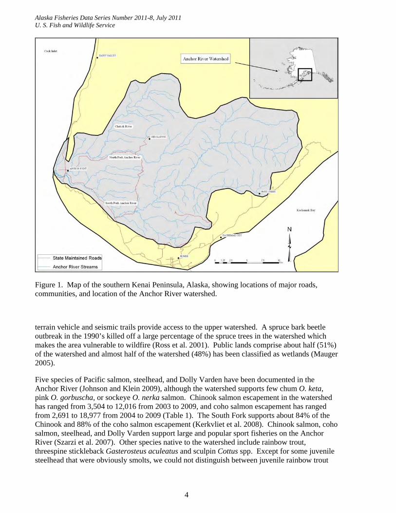
The Anchor River watershed (Figure 1) drains about 580 km2 of the lower Kenai Peninsula in southcentral Alaska (Mauger 2005). The watershed is non-glacial. The North and South forks of the Anchor River join to form a 5th order river about 3 km upstream from Cook Inlet, and the lower 2 km are influenced by tidal flows. The South Fork watershed is about twice the size of the North Fork watershed. Climate is characterized as a transitional zone between the maritime and continental zones and averages about 76 cm of precipitation that generally falls as snow between November and March (Kyle and Brabets 2001). Peak streamflows generally occur in April and May as snowmelt runoff, although rain events can cause peaks in discharge during summer and fall in some years (U. S. Geological Survey, unpublished data: http://waterdata.usgs.gov/nwis/nwisman/?site_no=15239900). For example, two significant flood events occurred during fall 2002 that caused heavy erosion, channelization, and damage to bridges and culverts. These events were caused by heavy rains and were in excess of any known or recorded event in the last 100 years (Szarzi et al. 2007).
Human activity is prevalent in the watershed and includes residential land use, gravel mining, logging, and recreation. Much of the lower watershed is accessible via roads, and numerous all-
Alaska Fisheries Data Series Number 2011-8, July 2011 U. S. Fish and Wildlife Service
4
Figure 1. Map of the southern Kenai Peninsula, Alaska, showing locations of major roads, communities, and location of the Anchor River watershed.
terrain vehicle and seismic trails provide access to the upper watershed. A spruce bark beetle outbreak in the 1990’s killed off a large percentage of the spruce trees in the watershed which makes the area vulnerable to wildfire (Ross et al. 2001). Public lands comprise about half (51%) of the watershed and almost half of the watershed (48%) has been classified as wetlands (Mauger 2005).
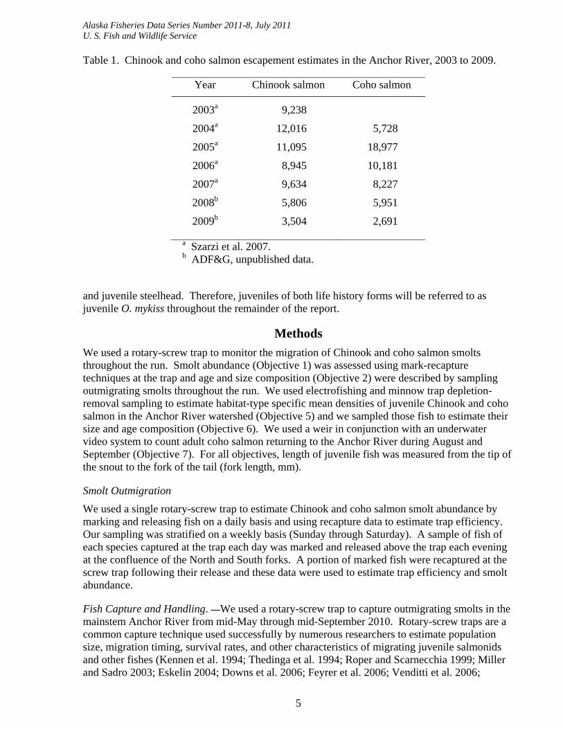
Five species of Pacific salmon, steelhead, and Dolly Varden have been documented in the Anchor River (Johnson and Klein 2009), although the watershed supports few chum O. keta, pink O. gorbuscha, or sockeye O. nerka salmon. Chinook salmon escapement in the watershed has ranged from 3,504 to 12,016 from 2003 to 2009, and coho salmon escapement has ranged from 2,691 to 18,977 from 2004 to 2009 (Table 1). The South Fork supports about 84% of the Chinook and 88% of the coho salmon escapement (Kerkvliet et al. 2008). Chinook salmon, coho salmon, steelhead, and Dolly Varden support large and popular sport fisheries on the Anchor River (Szarzi et al. 2007). Other species native to the watershed include rainbow trout, threespine stickleback Gasterosteus aculeatus and sculpin Cottus spp. Except for some juvenile steelhead that were obviously smolts, we could not distinguish between juvenile rainbow trout
Alaska Fisheries Data Series Number 2011-8, July 2011 U. S. Fish and Wildlife Service
5
Table 1. Chinook and coho salmon escapement estimates in the Anchor River, 2003 to 2009.
Year Chinook salmon Coho salmon
2003a 9,238
2004a 12,016 5,728
2005a 11,095 18,977
2006a 8,945 10,181
2007a 9,634 8,227
2008b 5,806 5,951
2009b 3,504 2,691
a Szarzi et al. 2007. b ADF&G, unpublished data.
and juvenile steelhead. Therefore, juveniles of both life history forms will be referred to as juvenile O. mykiss throughout the remainder of the report.
Methods
We used a rotary-screw trap to monitor the migration of Chinook and coho salmon smolts throughout the run. Smolt abundance (Objective 1) was assessed using mark-recapture techniques at the trap and age and size composition (Objective 2) were described by sampling outmigrating smolts throughout the run. We used electrofishing and minnow trap depletion-removal sampling to estimate habitat-type specific mean densities of juvenile Chinook and coho salmon in the Anchor River watershed (Objective 5) and we sampled those fish to estimate their size and age composition (Objective 6). We used a weir in conjunction with an underwater video system to count adult coho salmon returning to the Anchor River during August and September (Objective 7). For all objectives, length of juvenile fish was measured from the tip of the snout to the fork of the tail (fork length, mm).
Smolt Outmigration
We used a single rotary-screw trap to estimate Chinook and coho salmon smolt abundance by marking and releasing fish on a daily basis and using recapture data to estimate trap efficiency. Our sampling was stratified on a weekly basis (Sunday through Saturday). A sample of fish of each species captured at the trap each day was marked and released above the trap each evening at the confluence of the North and South forks. A portion of marked fish were recaptured at the screw trap following their release and these data were used to estimate trap efficiency and smolt abundance.
Fish Capture and Handling. —We used a rotary-screw trap to capture outmigrating smolts in the mainstem Anchor River from mid-May through mid-September 2010. Rotary-screw traps are a common capture technique used successfully by numerous researchers to estimate population size, migration timing, survival rates, and other characteristics of migrating juvenile salmonids and other fishes (Kennen et al. 1994; Thedinga et al. 1994; Roper and Scarnecchia 1999; Miller and Sadro 2003; Eskelin 2004; Downs et al. 2006; Feyrer et al. 2006; Venditti et al. 2006;
Alaska Fisheries Data Series Number 2011-8, July 2011 U. S. Fish and Wildlife Service
6
Volkhardt et al. 2007; Sykes et al. 2009). The trap consisted of a revolving stainless-steel, 2-mm-mesh cone on aluminum pontoons that was located below the confluence of the North and South forks near the Old Sterling Highway Bridge. The cone entrance diameter was 2.4 m and about half of the entrance area (about 2.2 m2) was submerged. Stream flow caused the trap cone to rotate and fish passing through the cone were collected in a live well located at the downstream end of the trap. The trap was secured to shore, placed in the thalweg to maximize capture efficiency, and was checked at least three times daily between 07:00 and 22:00 hours. When high water or debris caused concerns or when unusually high numbers of juveniles were passing, we checked the trap more frequently throughout the day and night. We raised the cone to stop fishing on three occasions during 2010 when high flows caused excessive turbulence in the live well that created stressful conditions for captured fish.
All fish captured at the screw trap were identified to species and counted. Chinook and coho salmon were classified as either smolt, parr, or transitional based on the presence or absence of parr marks and skin coloration as per Ewing et al. (1984) and Viola and Shuck (1995). Fish that were silver in coloration and had very faint or non-existent parr marks were classified as smolts, fish that were dark in coloration and had very distinct parr marks were classified as parr, and fish with characteristics of both smolt and parr (silver in coloration with distinct parr marks) were classified as transitional. Another characteristic used to distinguish smolts from parr or presmolts was the darkening of fin tips (Thedinga et al. 1994) or fin margin blackening (Wedemeyer et al. 1980). All Chinook and coho salmon captured at the trap were also examined for marks. All other non-marked and non-target fish captured in the smolt trap were identified to species and smolt stage (for salmonids), counted, placed in a live well, allowed to recover, and released once fish had recovered from handling. We noted any mortalities prior to release.
To estimate trap efficiency, up to 45 Chinook and 45 coho salmon classified as smolt or transitional each day were measured for length, marked according to Table 2 using surgical scissors cleaned with alcohol, and placed in 12-L buckets. Once sample size goals were obtained, marked fish were transferred from buckets to a live well near the release site and allowed to recover. Recovery time in the live well was usually about 8 to 10 hours, and all marked fish were released near dusk or by 2300 hours at the confluence of the North and South forks, about 100 m upstream of the screw trap. Any mortalities observed in the live well were noted prior to release of the marked fish.
Scale samples were collected from a sub-sample of captured fish that were not part of the trap efficiency trials, with a daily goal of up to 11 Chinook and coho salmon classified as smolt or transitional. This sample size goal was established such that simultaneous 90% C.I. estimates of the age composition for each species in each week would have a maximum width of 0.20 based on two age categories (Bromaghin 1993), and allowed for an estimated 15% unreadable scales. Fish selected for scale sample collection were anesthetized using a buffered tricaine methanesulfonate (MS-222) solution at a concentration of 40 mg/L (Schoettger and Julin 1967) with a target induction time of one to three minutes (CBFWA 1999) and measured for length. Scale “smears” were collected from the preferred area (Jearld 1983), but from the right side of the fish to minimize problems when scales are removed from the left side of returning adults. Scale samples were placed in individual coin envelopes and labeled with capture date, crew, capture method, location, species, length, and smolt stage. Scales were aged following the standards and guidelines of Mosher (1968), and juvenile ages are reported based on the number of winters the fish spent in fresh water followed by a plus sign (e.g., age 1+). Sampled fish were

Alaska Fisheries Data Series Number 2011-8, July 2011 U. S. Fish and Wildlife Service
7
Table 2. Stratum dates and partial caudal fin clips (top or bottom lobe) for Chinook and coho salmon smolts used to estimate trap efficiency.
Strata Dates Mark
1 3 – 5 June Top lobe
2 6 – 12 June Bottom lobe
3 13 – 19 June Top lobe
4 20 – 26 June Bottom lobe
5 27 June – 3
July Top lobe
6 4 – 10 July Bottom lobe
7 11 – 17 July Top lobe
8 18 – 24 July Bottom lobe
9 25 – 31 July Top lobe
10 1 – 7 August Bottom lobe
11 8 – 14 August Top lobe
12 15 – 19 August Bottom lobe
allowed to recover in a live well prior to release. We did not collect scale samples from fish marked as part of the trap efficiency experiment to minimize handling effects for those fish.
Data Analysis. —Chinook and coho salmon smolt abundance was estimated using a modification of a stratified mark-recapture design based on the recapture of marked smolts and trap efficiencies described by Carlson et al. (1998) using their equations and notations (below). Our main modification was to mark and release smolts each day during weekly strata instead of only marking and releasing fish once per stratum. For each stratum h, the smolt population size
excluding marked releases and observed mortality ( hU ) was estimated as
1
1ˆ
h
hhh m
MuU ,
where uh is the number of unmarked smolts captured in h, Mh is the number of marked smolts released in stratum h, and mh is the number of marked smolts recaptured in h. An unbiased
estimate of the variance of hU was calculated as
21
11ˆ2
hh
hhhhhhh
mm
umMmuMUv .
Total smolt abundance (U ) was estimated as
Alaska Fisheries Data Series Number 2011-8, July 2011 U. S. Fish and Wildlife Service
8
L
hhUU
1
ˆˆ ,
where L is the number of strata, and the variance estimate was calculated as
L
hhUvUv
1
ˆˆ .
An approximate 90% C.I. was calculated as
UvU ˆ645.1ˆ .
We set our goal for Mh at 300 fish of each species based on Equation 22 of Carlson et al. (1998) with assumptions of a 15% trap efficiency, a relative error of 25%, and α = 0.10. Marking and releasing 45 fish each day allowed us to achieve this goal during most weekly strata. We assumed that fish marked in a given temporal stratum were recaptured within the same stratum, as has been observed by many researchers (Thedinga et al. 1994; Roper and Scarnecchia 1996; Roper and Scarnecchia 1999; Eskelin 2004; Steinhorst et al. 2004). However, we applied two alternating marks over the course of the season (Table 2) to investigate this assumption. Only fish classified as smolt or transitional were marked.
Assumptions associated with each stratum for the above method are (from Carlson et al. 1998): 1) closed population; 2) all smolts have the same probability of being marked or all smolts have the same probability of being examined for marks; 3) constant capture probability; 4) marks are not lost between release and recovery; 5) all marked smolts are reported; and 6) all marked smolts released are either recovered or pass by the downstream capture site. Basic data summaries, scatter plots, and statistical analyses were used to describe characteristics of captured smolts and to investigate the validity of assumptions. Assumption 1 was probably met in most strata, and mortality observed during handling and marking was minimal and was censored from the estimate. Assumption 2 involves potential problems associated with random sampling, mixing of marked and unmarked smolts, and variable catchability based on size selectivity, marking effects, or other factors. We addressed this assumption by randomly netting our daily marking sample from the live well when possible. At times, it was necessary to mark all fish captured in the live well to achieve daily sample size goals. Also, we selected a release site at the confluence of the North and South forks that was about 100 m upstream of the trap to maximize the probability that marked fish were able to mix with the general population prior to recapture (Seelbach et al. 1985; Thedinga et al. 1994). We also investigated size selectivity by comparing lengths of marked and recaptured fish using a Kolmogorov-Smirnov two-sample test (Sokal and Rohlf 1981). Assumption 3 requires trap efficiency to be constant within each stratum. Many factors can influence trap efficiency including time of release and turbidity (Eskelin 2004), changing stream flow conditions (Volkhardt et al. 2007), fish size and species (Thedinga et al. 1994; Volkhardt et al. 2007), and changes to how the trap is operated (e.g., moved to different positions, addition of screen panels). Marking and releasing fish on a daily basis allowed us to investigate the influence of these variables on capture efficiency. The partial caudal fin-clips used as marks were clearly visible to the crew when recaptured at the screw trap and did not regenerate in the short time period between release and recovery (Assumption 4), and the crew was properly trained in fish handling and marking techniques and followed procedures to ensure all captured fish were examined for marks and all marks were reported (Assumption 5). To address Assumption 6, we only marked and released fish classified as smolt or transitional,
Alaska Fisheries Data Series Number 2011-8, July 2011 U. S. Fish and Wildlife Service
9
and we expected most marked smolts to migrate past the trap shortly after their release (Thedinga et al. 1994; Roper and Scarnecchia 1996; Roper and Scarnecchia 1999; Eskelin 2004; Steinhorst et al. 2004).
We used stage height data from the U. S. Geological Survey stream gage site on the South Fork Anchor River, air and water temperature data from the Cook Inletkeeper monitoring program (Sue Mauger, Cook Inletkeeper, personal communication), and trap revolutions-per-minute (RPM) to investigate correlations with trap efficiency using basic data summaries, scatter plots, and statistical analyses. We summarized hourly stage height data and used mean daily stage height in all analyses.
Smolt-to-Spawning Adult Return Rate
We will estimate coho salmon smolt-to-spawning adult return rate by dividing the count of adult coho salmon returning to the Anchor River weir in 2011 by the 2010 smolt abundance estimate
(U ) and variance will be calculated using the Delta method (Seber 1982). This estimate will account for both fishing and natural mortality, but we will not be able to separate the two components. This estimate is possible because of the relatively simple marine life history of coho salmon in that nearly all smolts from 2010 will only spend one winter in the ocean before returning as adults in 2011 (Sandercock 1991). The smolt-to-spawning adult return estimate assumes our count of adult coho salmon returning to the Anchor River is a complete census, which we expect to achieve using the weir and underwater video technology (Anderson et al. 2006; Gates and Boersma 2009).
Juvenile Habitat Use
The goal of the habitat use sampling was to describe fish use by habitat type throughout the Anchor River watershed and to describe habitat composition at each of the study reaches, both important parameters of the RIPPLE model. We accomplished this by estimating abundance of fish in individual habitat units using depletion sampling with two gear types (minnow traps and electrofishing) and dividing the abundance estimate by the surface area of the unit to calculate densities as number of fish/m2.
Sample locations within the Anchor River watershed were chosen using a digital stream network produced by Stillwater Sciences using a high resolution DEM. The stream network was stratified by slope class (%) and drainage area (km2) within each slope class. Drainage area was determined by calculating watershed area upstream of each channel reach. We also distinguished sites within the Chakok River sub-watershed for separate analysis in RIPPLE based on observed differences in channel morphology (sinuosity, channel form) from the rest of the Anchor River watershed. Sample reaches were distributed throughout the watershed as much as practical, but accessibility also guided site selection. Within each slope class and sub-watershed, we chose sample reaches that were: 1) accessible within about 1 km from the road system or established trails; 2) on public land or on private land where we could obtain permission to trespass; 3) in areas where we expected to find juvenile salmonids based on Johnson and Klein (2009); and 4) representative of the different drainage area classes. Stream reaches were accessed using the most direct route possible and permission from landowners was secured in advance when accessing private property. Sampling at each reach involved collection of fish and aquatic habitat parameters at selected habitat units.
Alaska Fisheries Data Series Number 2011-8, July 2011 U. S. Fish and Wildlife Service
10
At each sample reach, we attempted to sample fish in different habitat types. A sample size goal of n = 5 reaches per slope class was selected based on simulation testing where we considered four parameters for modeling sample sizes for fish capture: 1) the probability of capture in each depletion pass; 2) the true mean population density expressed as number of fish per habitat unit – this is equivalent to assuming all habitat units are about the same size; 3) the variability in population density among habitat units expressed as a dispersion coefficient – in this case the ratio of the standard deviation to the mean; and 4) the number of habitat units sampled. For each set of parameters, we generated densities for each survey unit by sampling from a lognormal distribution with the given mean and dispersion coefficient. Then a four-pass depletion sampling was simulated from each unit using the jackknife estimator of Pollock and Otto (1983) to estimate the populations of individual units and formulas from Hankin (1984) to expand these to the study reach. Four passes were chosen for our modeling since we chose to use four electrofishing or minnow trap removal events to test capture probability assumptions for removal models presented that are discussed below. Simulations were repeated 1,000 times to build up a population of estimated densities from which the 90% bounds on relative error were calculated.
The basic conclusion is that the variability in density from unit to unit is the most important factor. If the dispersion coefficient is 1, there is no realistic hope of attaining the desired performance level with any reasonable amount of sampling. If the dispersion coefficient is no more than 20%, five sample reaches per slope class suffices to meet Objective 5 under almost all combinations of the other parameters. Appendix A presents a summary of modeling results based on capture probabilities of 40% and 80% and a dispersion coefficient of 0.20.
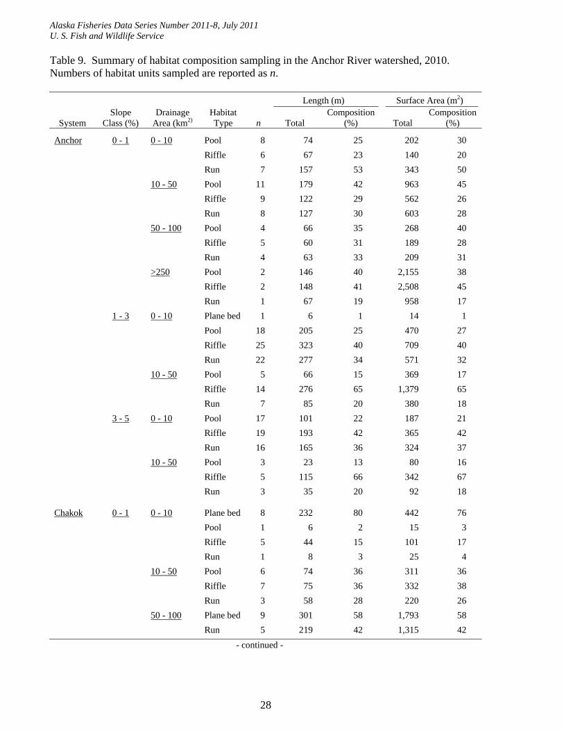
Sample reaches were classified following a scheme based on Montgomery and Buffington (1997) which uses channel slope to define processed-based channel reach types; this approach is in accord with the methods used in the RIPPLE model. Individual habitat units within each reach were classified as pool, riffle, run, or plane-bed habitat types based on definitions modified from Bisson et al. (1982), Hankin and Reeves (1988), Montgomery and Buffington (1997), and Overton et al. (1997). Pools were defined as areas with reduced current velocity, often with water deeper than surrounding areas, typically formed by scouring water that has carved out a non-uniform depression in the channel bed or a dam. Runs were defined as deep and fast areas with a defined thalweg and little surface agitation where flow obstructions in the form of boulders may be present. Riffles were defined as shallow areas where water flows swiftly over completely or partially submerged obstructions to produce surface agitation. Plane-bed habitats were defined as long stretches of relatively featureless bed without organized bedforms. Reach lengths were set at 40 wetted channel widths for streams greater than or equal to 3.75 m wide and reach lengths were set at 150 m for streams less than 3.75 m wide (Reynolds et al. 2003). Maximum reach length was limited to 300 m for streams greater than 7.5 m wide to place a maximum effort threshold for each individual sampling reach. Habitat composition within each reach was estimated by beginning at the downstream end of the reach and working upstream for the predetermined reach length. Individual habitat units were classified based on habitat type, and length (m) was measured along the thalweg. A minimum of three widths were measured perpendicular to the thalweg at cross-sections spaced at ¼, ½, and ¾ of the unit's length, and a mean width (m) was calculated. Surface area of each habitat unit was calculated by multiplying the measured length of the unit by its mean width. Percent composition of each habitat type was summarized by length and surface area for each sample reach.
The spatial coordinates of the downstream end of each sampled reach were recorded in decimal degrees with a handheld global positioning system using the North American Datum of 1983
Alaska Fisheries Data Series Number 2011-8, July 2011 U. S. Fish and Wildlife Service
11
(NAD83) geographic coordinate system. Water temperature (°C) was measured with a hand-held thermometer and conductivity (μS/cm) for reaches where we sampled with electrofishing was measured using a YSI Model 85 water quality meter.
Fish sampling was conducted using electrofishing and minnow traps and the gear type was selected based on stream order (Strahler 1952) which was determined from the digital stream channel network prior to sampling. Electrofishing was only conducted in first or second order streams that flowed into streams no higher than order three to minimize impacts to adult fish.
Regardless of capture method, juvenile salmonids and other non-target fish were identified to species (Pollard et al. 1997), counted, measured for length, and placed in live wells. Scale samples were collected from all juvenile coho salmon greater than 70 mm in length. We assumed most coho salmon less than 70 mm in length were age 0+ fish based on sampling in other southern Alaska streams (Anderson and Hetrick 2004). Fish were anesthetized and scale samples were collected as previously described. Sampled fish were allowed to recover in a live well prior to release.
Electrofishing. —A Smith-Root backpack electrofisher (Model LR-24 or Model 15) was used by a Service-certified operator following the safety guidelines outlined in Reynolds (1996) and USFWS (2004). Output voltage was adjusted to the minimum level necessary to achieve electrotaxis (forced swimming) and pulsed DC was used to minimize fish injury (Dalbey et al. 1996). Electrical output parameters (voltage, current, and power) were recorded along with conductivity (μS/cm) at each location. A visual reconnaissance of each habitat unit was conducted prior to sampling to verify the absence of adult salmonids, and sampling immediately ceased if large salmonids (> 200 mm) were encountered. One person operated the backpack electrofisher and two crew members netted fish.
We used four equal-effort electrofishing removal passes that allowed us to test assumptions of equal capture probability (White et al. 1982). To assure equal sampling effort, all habitat was thoroughly electrofished on each pass (Riley and Fausch 1992). Block nets were placed at the upstream and downstream ends of the habitat units to prevent immigration and emigration of fish during the removal events. After each electrofishing pass, juvenile fish were processed as described above and placed in live wells. After all passes were completed, block nets were removed and all fish were returned to the habitat unit of capture. We noted any mortalities caused by electrofishing.
Minnow Traps. —Minnow traps were used to capture and remove fish from selected habitat units following the procedures of Bryant (2000). Block nets were placed at the upstream and downstream ends of the habitat units to prevent immigration and emigration of fish during the removal events. Four capture events were used in each habitat unit so that we could test assumptions of equal capture probability (White et al. 1982). Between eight and 20 minnow traps were set during each event depending on the size of the habitat unit. Distances between traps depended on habitat complexity, but traps were generally separated by about 1.5 m. Traps were set more densely in complex habitats. Traps were set on the stream bottom near large woody debris, root wads, or undercut banks where juvenile salmonids were expected to be present, but were also distributed over the entire habitat unit. Traps were baited with salmon eggs that had been disinfected by soaking for at least 10 minutes in a 1/100 Betadyne solution and placed in a perforated plastic bag. Traps remained undisturbed for 60 5 minutes, and picked up in the order in which they were set. Juvenile fishes were removed from the traps
Alaska Fisheries Data Series Number 2011-8, July 2011 U. S. Fish and Wildlife Service
12
between capture occasions and processed as described above, and traps were re-set in their original locations. The procedure was repeated for four capture occasions. After all passes were completed, block nets were removed and all fish were returned to the habitat unit of capture. We noted any mortalities.
Data Analysis. —Removal estimates and probabilities of capture for electrofishing and minnow trap experiments were computed by Program CAPTURE (White et al. 1982). Program CAPTURE uses catch data from depletion sampling to estimate sampling efficiency and population size, and uses two different models to generate population estimates. The first model is equivalent to the trap response model for a closed population (Mb; Pollock et al. 1990) and is based on the assumption of a constant capture probability for all capture events. The second model is equivalent to a heterogeneity and trap response model for a closed population (Mbh; Pollock et al. 1990) and is based on the assumption of two different capture probabilities: one for the first capture event and a different probability for the remaining capture events. Program CAPTURE performs a chi-square goodness of fit test for each model to determine whether observed capture probabilities follow those expected for either model. Our four removal events were sufficient to test capture probability assumptions for both models. White et al. (1982) recommend using model results only if probabilities for the model chi-square goodness of fit test were at least 0.20 to avoid bias. The model selected by Program CAPTURE was chosen for analysis purposes, and models were scrutinized if either P < 0.20 for any model goodness of fit test, observed capture probabilities were less than 0.20, or population size was less than 200 individuals (White et al. 1982).
Density (number of fish/m2) for each habitat unit was calculated by dividing the population estimate by the surface area of the unit. Relative density (number of fish/m2) was also reported for each habitat unit as the total number of fish captured in all passes divided by the surface area. Mean densities and mean relative densities by habitat type, slope class, and drainage area were summarized for use as parameters in the RIPPLE model. The variance associated with the mean density estimates will be used to guide future sampling. Basic data summaries, scatter plots, and statistical analyses were used to describe characteristics of sampled fish. Length-frequency distributions and age composition were compared among and between habitat types and slope classes for each species.
Adult Escapement
We operated the ADF&G floating resistance board weir to count adult coho salmon returning to the Anchor River. The weir design and operation is described by Kerkvliet et al. (2008), and we incorporated an underwater video system similar to that described by Gates and Boersma (2009). Power for the underwater video system was provided by a combination of 12-VDC deep cycle batteries and a gasoline-powered generator. An underwater video camera was placed inside a sealed video box attached to the fish passage chute. The video box was constructed of 3.2-mm aluminum sheeting and filled with filtered water. Safety glass was installed on the front of the video box to allow for a scratch-free, clear surface through which images were captured. The passage chute was constructed from aluminum angle and enclosed in plywood which isolated it from exterior light. The backdrop of the passage chute from which video images were captured was adjusted laterally to minimize the number of fish passing through the chute at one time. The video box and fish passage chute were artificially lit using a pair of 12-VDC underwater pond lights. Pond lights were equipped with 20-W bulbs which produced a quality image and provided a consistent source of lighting during day and night hours. All video images were recorded on an external 500 gigabyte hard drive at 30 frames-per-second using a computer-based
Alaska Fisheries Data Series Number 2011-8, July 2011 U. S. Fish and Wildlife Service
13
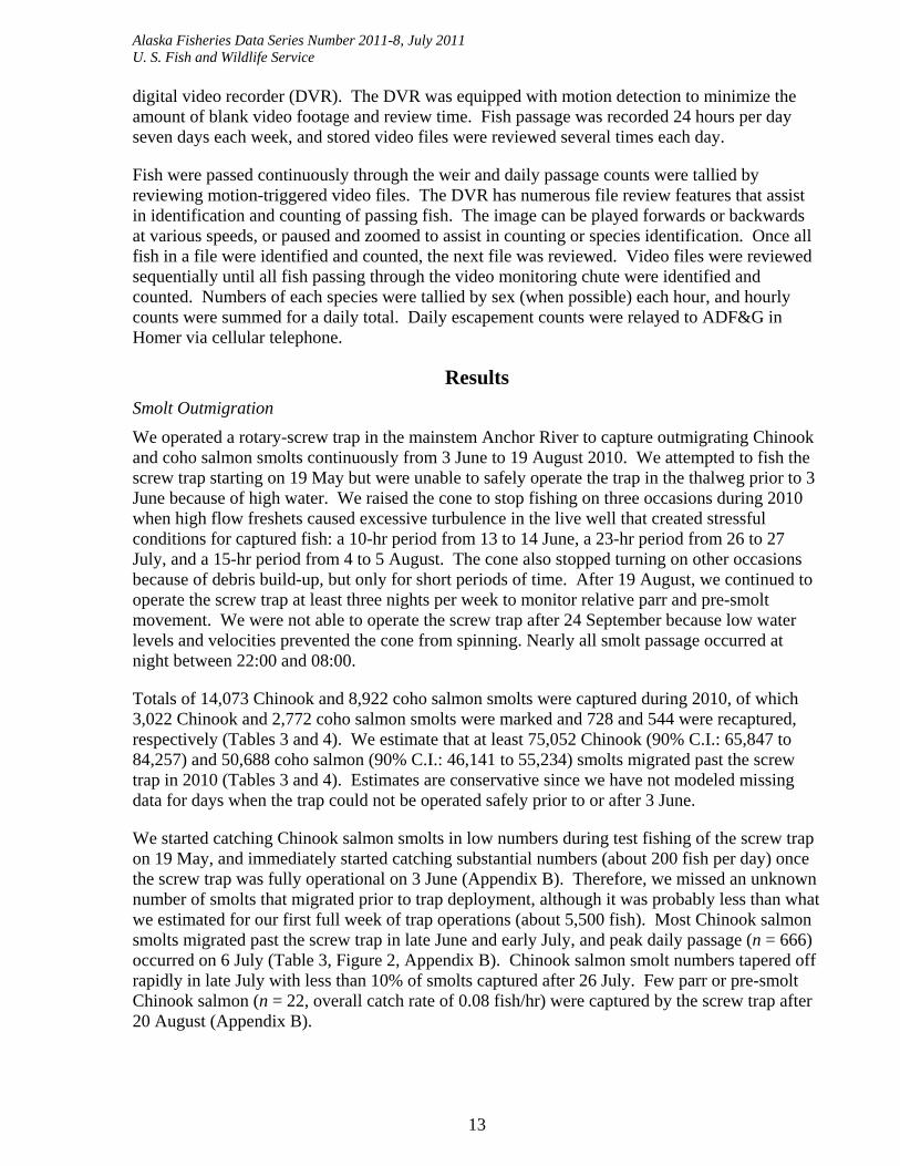
digital video recorder (DVR). The DVR was equipped with motion detection to minimize the amount of blank video footage and review time. Fish passage was recorded 24 hours per day seven days each week, and stored video files were reviewed several times each day.
Fish were passed continuously through the weir and daily passage counts were tallied by reviewing motion-triggered video files. The DVR has numerous file review features that assist in identification and counting of passing fish. The image can be played forwards or backwards at various speeds, or paused and zoomed to assist in counting or species identification. Once all fish in a file were identified and counted, the next file was reviewed. Video files were reviewed sequentially until all fish passing through the video monitoring chute were identified and counted. Numbers of each species were tallied by sex (when possible) each hour, and hourly counts were summed for a daily total. Daily escapement counts were relayed to ADF&G in Homer via cellular telephone.
Results
Smolt Outmigration
We operated a rotary-screw trap in the mainstem Anchor River to capture outmigrating Chinook and coho salmon smolts continuously from 3 June to 19 August 2010. We attempted to fish the screw trap starting on 19 May but were unable to safely operate the trap in the thalweg prior to 3 June because of high water. We raised the cone to stop fishing on three occasions during 2010 when high flow freshets caused excessive turbulence in the live well that created stressful conditions for captured fish: a 10-hr period from 13 to 14 June, a 23-hr period from 26 to 27 July, and a 15-hr period from 4 to 5 August. The cone also stopped turning on other occasions because of debris build-up, but only for short periods of time. After 19 August, we continued to operate the screw trap at least three nights per week to monitor relative parr and pre-smolt movement. We were not able to operate the screw trap after 24 September because low water levels and velocities prevented the cone from spinning. Nearly all smolt passage occurred at night between 22:00 and 08:00.
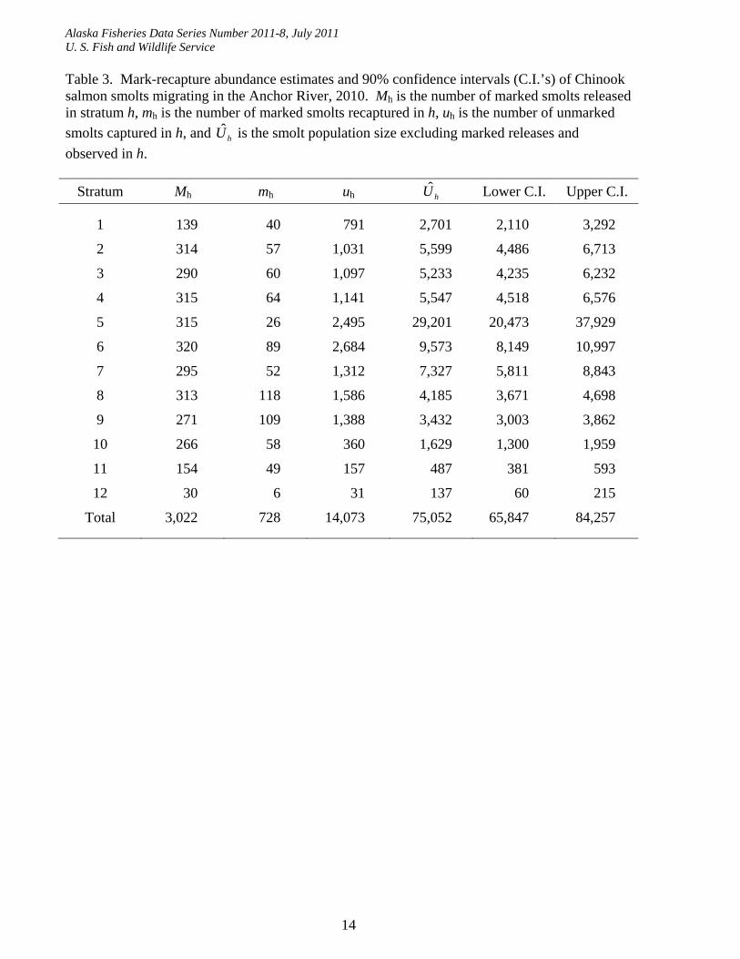
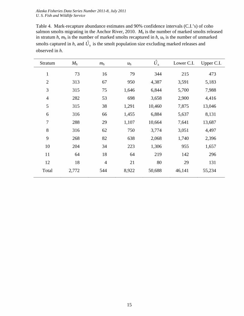
Totals of 14,073 Chinook and 8,922 coho salmon smolts were captured during 2010, of which 3,022 Chinook and 2,772 coho salmon smolts were marked and 728 and 544 were recaptured, respectively (Tables 3 and 4). We estimate that at least 75,052 Chinook (90% C.I.: 65,847 to 84,257) and 50,688 coho salmon (90% C.I.: 46,141 to 55,234) smolts migrated past the screw trap in 2010 (Tables 3 and 4). Estimates are conservative since we have not modeled missing data for days when the trap could not be operated safely prior to or after 3 June.
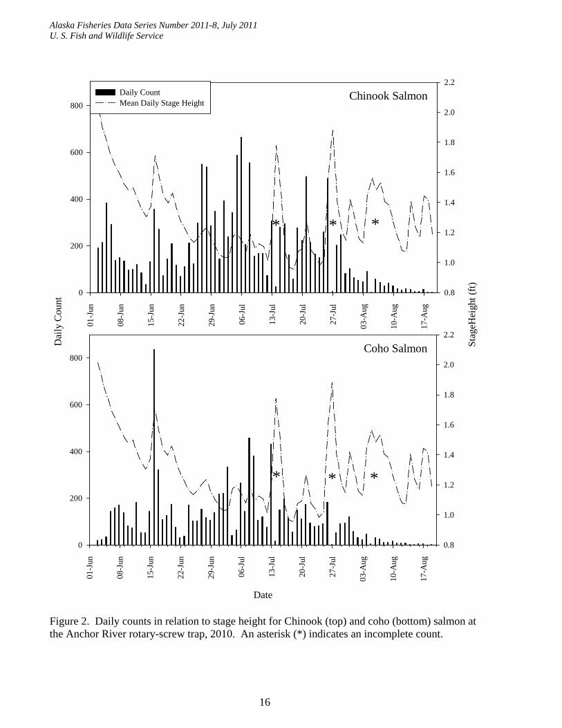
We started catching Chinook salmon smolts in low numbers during test fishing of the screw trap on 19 May, and immediately started catching substantial numbers (about 200 fish per day) once the screw trap was fully operational on 3 June (Appendix B). Therefore, we missed an unknown number of smolts that migrated prior to trap deployment, although it was probably less than what we estimated for our first full week of trap operations (about 5,500 fish). Most Chinook salmon smolts migrated past the screw trap in late June and early July, and peak daily passage (n = 666) occurred on 6 July (Table 3, Figure 2, Appendix B). Chinook salmon smolt numbers tapered off rapidly in late July with less than 10% of smolts captured after 26 July. Few parr or pre-smolt Chinook salmon (n = 22, overall catch rate of 0.08 fish/hr) were captured by the screw trap after 20 August (Appendix B).
Alaska Fisheries Data Series Number 2011-8, July 2011 U. S. Fish and Wildlife Service
14
Table 3. Mark-recapture abundance estimates and 90% confidence intervals (C.I.’s) of Chinook salmon smolts migrating in the Anchor River, 2010. Mh is the number of marked smolts released in stratum h, mh is the number of marked smolts recaptured in h, uh is the number of unmarked
smolts captured in h, and hU is the smolt population size excluding marked releases and
observed in h.
Stratum Mh mh uh hU Lower C.I. Upper C.I.
1 139 40 791 2,701 2,110 3,292
2 314 57 1,031 5,599 4,486 6,713
3 290 60 1,097 5,233 4,235 6,232
4 315 64 1,141 5,547 4,518 6,576
5 315 26 2,495 29,201 20,473 37,929
6 320 89 2,684 9,573 8,149 10,997
7 295 52 1,312 7,327 5,811 8,843
8 313 118 1,586 4,185 3,671 4,698
9 271 109 1,388 3,432 3,003 3,862
10 266 58 360 1,629 1,300 1,959
11 154 49 157 487 381 593
12 30 6 31 137 60 215
Total 3,022 728 14,073 75,052 65,847 84,257
Alaska Fisheries Data Series Number 2011-8, July 2011 U. S. Fish and Wildlife Service
15
Table 4. Mark-recapture abundance estimates and 90% confidence intervals (C.I.’s) of coho salmon smolts migrating in the Anchor River, 2010. Mh is the number of marked smolts released in stratum h, mh is the number of marked smolts recaptured in h, uh is the number of unmarked
smolts captured in h, and hU is the smolt population size excluding marked releases and
observed in h.
Stratum Mh mh uh hU Lower C.I. Upper C.I.
1 73 16 79 344 215 473
2 313 67 950 4,387 3,591 5,183
3 315 75 1,646 6,844 5,700 7,988
4 282 53 698 3,658 2,900 4,416
5 315 38 1,291 10,460 7,875 13,046
6 316 66 1,455 6,884 5,637 8,131
7 288 29 1,107 10,664 7,641 13,687
8 316 62 750 3,774 3,051 4,497
9 268 82 638 2,068 1,740 2,396
10 204 34 223 1,306 955 1,657
11 64 18 64 219 142 296
12 18 4 21 80 29 131
Total 2,772 544 8,922 50,688 46,141 55,234
Alaska Fisheries Data Series Number 2011-8, July 2011 U. S. Fish and Wildlife Service
16
Chinook Salmon01
-Jun
08-J
un
15-J
un
22-J
un
29-J
un
06-J
ul
13-J
ul
20-J
ul
27-J
ul
03-A
ug
10-A
ug
17-A
ug
Dai
ly C
ount
0
200
400
600
800
Sta
geH
eigh
t (ft
)
0.8
1.0
1.2
1.4
1.6
1.8
2.0
2.2Daily CountMean Daily Stage Height
Coho Salmon
Date
01-J
un
08-J
un
15-J
un
22-J
un
29-J
un
06-J
ul
13-J
ul
20-J
ul
27-J
ul
03-A
ug
10-A
ug
17-A
ug
0
200
400
600
800
0.8
1.0
1.2
1.4
1.6
1.8
2.0
2.2
** *
* * *
Figure 2. Daily counts in relation to stage height for Chinook (top) and coho (bottom) salmon at the Anchor River rotary-screw trap, 2010. An asterisk (*) indicates an incomplete count.
Alaska Fisheries Data Series Number 2011-8, July 2011 U. S. Fish and Wildlife Service
17
We did not catch coho salmon in large numbers until after the trap was fully operational on 3 June, so we assume we sampled during the entire coho salmon smolt outmigration. Most coho salmon smolts migrated past the screw trap in late June and early July, although peak daily passage (n = 838) occurred on 16 June (Table 4, Figure 2, Appendix B). Coho salmon smolt numbers also tapered off rapidly in late July with less than 10% of smolts captured after 25 July. Relatively few parr or pre-smolt coho salmon (n = 109, overall catch rate of 0.41 fish/hr) were captured by the screw trap after 20 August (Appendix B).
In addition to Chinook and coho salmon, other species captured in the screw trap included pink and sockeye salmon; Dolly Varden smolts, parr, and adults; steelhead smolts and adult kelts; juvenile O. mykiss, threespine stickleback, lamprey Lampetra spp., eulachon Thaleichthys pacificus, and sculpin. Dolly Varden smolts passed the screw trap in early June and steelhead smolt passage occurred in July (Appendix B).
Mark-recapture assumptions for the screw trap capture efficiency estimates were valid most of the time, and the methods we adopted to address assumptions were described above. Mortality of tagged fish (Assumption 1) was low overall, and totals of n = 22 marked Chinook salmon (0.7% of total marked) and n = 12 marked coho salmon (0.4% of total marked) were mortalities observed in the release site live well. These mortalities were subtracted from the marked total in their respective strata. Most mortality occurred on two occasions; the first mortality event (n = 8 Chinook salmon and n = 4 coho salmon) occurred when the crew was experimenting with locating the release live well behind the rotary-screw trap and an unexpected vortex formed inside of the live well that trapped fish against the sides. The second mortality event (n = 4 Chinook salmon and n = 6 coho salmon) occurred when debris accumulated in the release site live well.
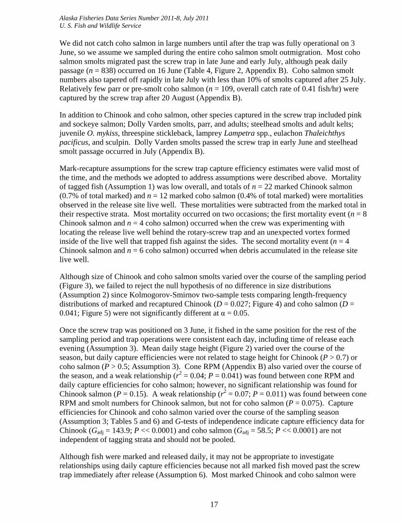
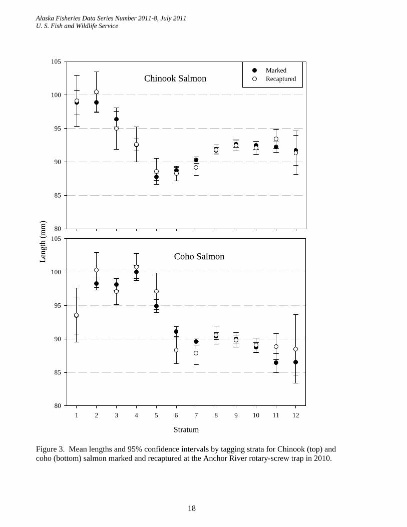
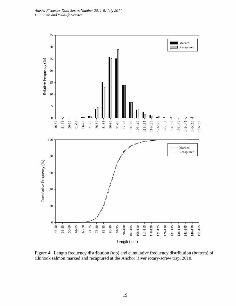
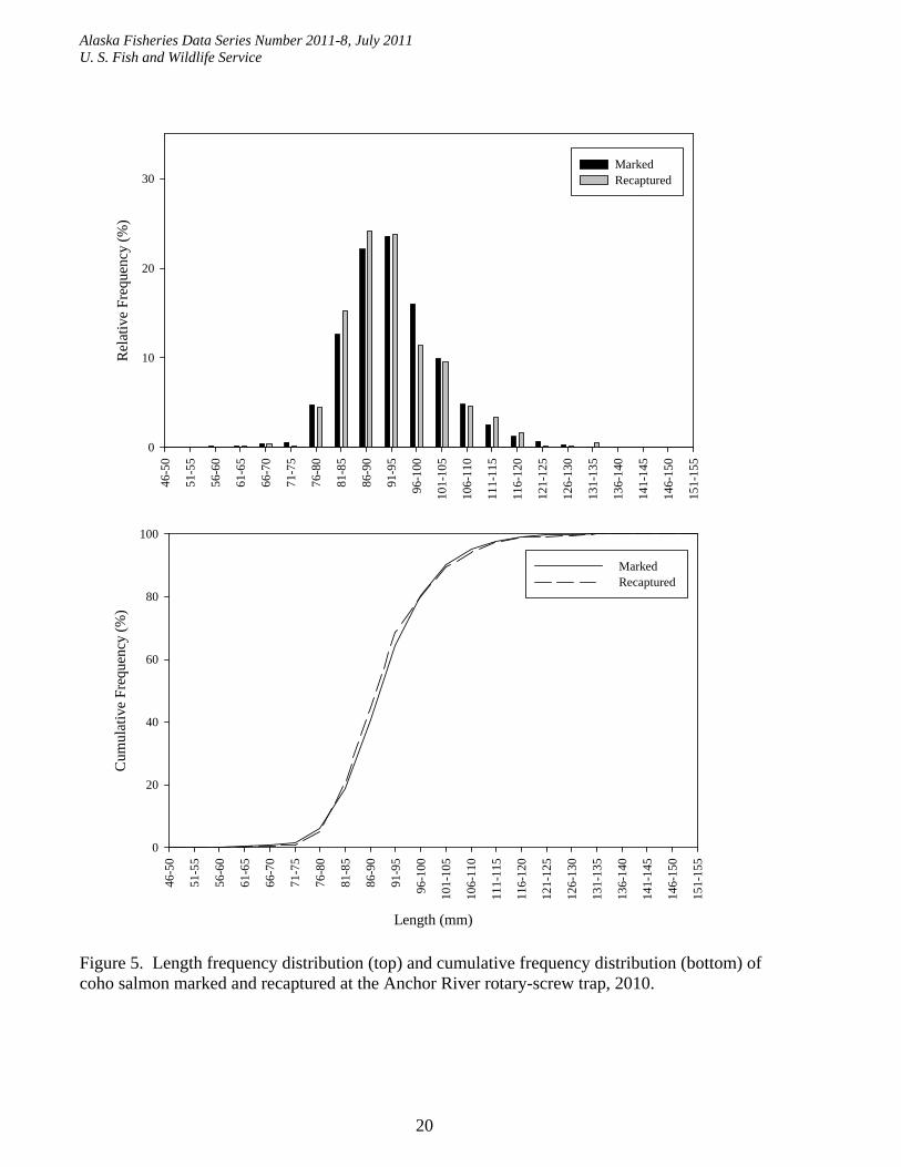
Although size of Chinook and coho salmon smolts varied over the course of the sampling period (Figure 3), we failed to reject the null hypothesis of no difference in size distributions (Assumption 2) since Kolmogorov-Smirnov two-sample tests comparing length-frequency distributions of marked and recaptured Chinook (D = 0.027; Figure 4) and coho salmon (D = 0.041; Figure 5) were not significantly different at α = 0.05.
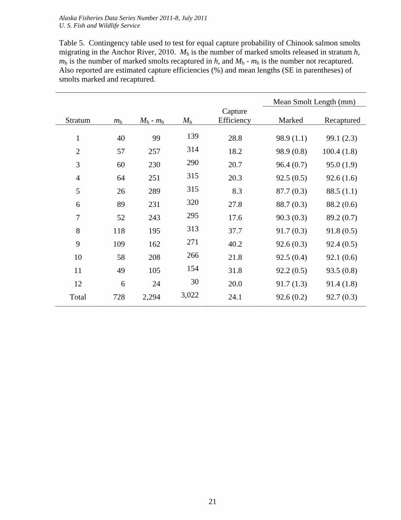
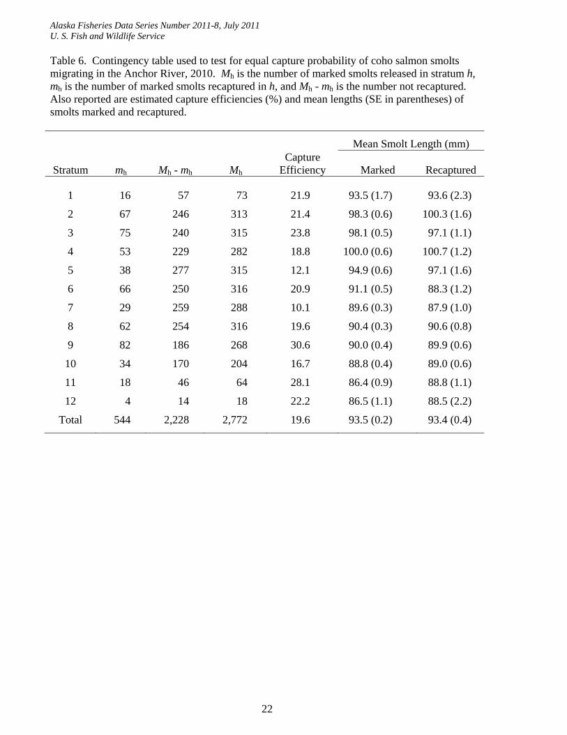
Once the screw trap was positioned on 3 June, it fished in the same position for the rest of the sampling period and trap operations were consistent each day, including time of release each evening (Assumption 3). Mean daily stage height (Figure 2) varied over the course of the season, but daily capture efficiencies were not related to stage height for Chinook (P > 0.7) or coho salmon (P > 0.5; Assumption 3). Cone RPM (Appendix B) also varied over the course of the season, and a weak relationship (r2 = 0.04; P = 0.041) was found between cone RPM and daily capture efficiencies for coho salmon; however, no significant relationship was found for Chinook salmon (P = 0.15). A weak relationship (r2 = 0.07; P = 0.011) was found between cone RPM and smolt numbers for Chinook salmon, but not for coho salmon (P = 0.075). Capture efficiencies for Chinook and coho salmon varied over the course of the sampling season (Assumption 3; Tables 5 and 6) and G-tests of independence indicate capture efficiency data for Chinook (Gadj = 143.9; P << 0.0001) and coho salmon (Gadj = 58.5; P << 0.0001) are not independent of tagging strata and should not be pooled.
Although fish were marked and released daily, it may not be appropriate to investigate relationships using daily capture efficiencies because not all marked fish moved past the screw trap immediately after release (Assumption 6). Most marked Chinook and coho salmon were
Alaska Fisheries Data Series Number 2011-8, July 2011 U. S. Fish and Wildlife Service
18
Chinook Salmon
Len
gth
(mm
)
80
85
90
95
100
105Marked Recaptured
Coho Salmon
Stratum
1 2 3 4 5 6 7 8 9 10 11 12
80
85
90
95
100
105
Figure 3. Mean lengths and 95% confidence intervals by tagging strata for Chinook (top) and coho (bottom) salmon marked and recaptured at the Anchor River rotary-screw trap in 2010.
Alaska Fisheries Data Series Number 2011-8, July 2011 U. S. Fish and Wildlife Service
19
46-5
0
51-5
5
56-6
0
61-6
5
66-7
0
71-7
5
76-8
0
81-8
5
86-9
0
91-9
5
96-1
00
101-
105
106-
110
111-
115
116-
120
121-
125
126-
130
131-
135
136-
140
141-
145
146-
150
151-
155
Rel
ativ
e Fr
eque
ncy
(%)
0
5
10
15
20
25
30
35
Marked Recaptured
Length (mm)
46-5
0
51-5
5
56-6
0
61-6
5
66-7
0
71-7
5
76-8
0
81-8
5
86-9
0
91-9
5
96-1
00
101-
105
106-
110
111-
115
116-
120
121-
125
126-
130
131-
135
136-
140
141-
145
146-
150
151-
155
Cum
ulat
ive
Freq
uenc
y (%
)
0
20
40
60
80
100
Marked Recaptured
Figure 4. Length frequency distribution (top) and cumulative frequency distribution (bottom) of Chinook salmon marked and recaptured at the Anchor River rotary-screw trap, 2010.
Alaska Fisheries Data Series Number 2011-8, July 2011 U. S. Fish and Wildlife Service
20
46-5
0
51-5
5
56-6
0
61-6
5
66-7
0
71-7
5
76-8
0
81-8
5
86-9
0
91-9
5
96-1
00
101-
105
106-
110
111-
115
116-
120
121-
125
126-
130
131-
135
136-
140
141-
145
146-
150
151-
155
Rel
ativ
e Fr
eque
ncy
(%)
0
10
20
30Marked Recaptured
Length (mm)
46-5
0
51-5
5
56-6
0
61-6
5
66-7
0
71-7
5
76-8
0
81-8
5
86-9
0
91-9
5
96-1
00
101-
105
106-
110
111-
115
116-
120
121-
125
126-
130
131-
135
136-
140
141-
145
146-
150
151-
155
Cum
ulat
ive
Freq
uenc
y (%
)
0
20
40
60
80
100
Marked Recaptured
Figure 5. Length frequency distribution (top) and cumulative frequency distribution (bottom) of coho salmon marked and recaptured at the Anchor River rotary-screw trap, 2010.
Alaska Fisheries Data Series Number 2011-8, July 2011 U. S. Fish and Wildlife Service
21
Table 5. Contingency table used to test for equal capture probability of Chinook salmon smolts migrating in the Anchor River, 2010. Mh is the number of marked smolts released in stratum h, mh is the number of marked smolts recaptured in h, and Mh - mh is the number not recaptured. Also reported are estimated capture efficiencies (%) and mean lengths (SE in parentheses) of smolts marked and recaptured.
Mean Smolt Length (mm)
Stratum mh Mh - mh Mh Capture
Efficiency Marked Recaptured
1 40 99 139 28.8 98.9 (1.1) 99.1 (2.3)
2 57 257 314 18.2 98.9 (0.8) 100.4 (1.8)
3 60 230 290 20.7 96.4 (0.7) 95.0 (1.9)
4 64 251 315 20.3 92.5 (0.5) 92.6 (1.6)
5 26 289 315 8.3 87.7 (0.3) 88.5 (1.1)
6 89 231 320 27.8 88.7 (0.3) 88.2 (0.6)
7 52 243 295 17.6 90.3 (0.3) 89.2 (0.7)
8 118 195 313 37.7 91.7 (0.3) 91.8 (0.5)
9 109 162 271 40.2 92.6 (0.3) 92.4 (0.5)
10 58 208 266 21.8 92.5 (0.4) 92.1 (0.6)
11 49 105 154 31.8 92.2 (0.5) 93.5 (0.8)
12 6 24 30 20.0 91.7 (1.3) 91.4 (1.8)
Total 728 2,294 3,022 24.1 92.6 (0.2) 92.7 (0.3)
Alaska Fisheries Data Series Number 2011-8, July 2011 U. S. Fish and Wildlife Service
22
Table 6. Contingency table used to test for equal capture probability of coho salmon smolts migrating in the Anchor River, 2010. Mh is the number of marked smolts released in stratum h, mh is the number of marked smolts recaptured in h, and Mh - mh is the number not recaptured. Also reported are estimated capture efficiencies (%) and mean lengths (SE in parentheses) of smolts marked and recaptured.
Mean Smolt Length (mm)
Stratum mh Mh - mh Mh Capture
Efficiency Marked Recaptured
1 16 57 73 21.9 93.5 (1.7) 93.6 (2.3)
2 67 246 313 21.4 98.3 (0.6) 100.3 (1.6)
3 75 240 315 23.8 98.1 (0.5) 97.1 (1.1)
4 53 229 282 18.8 100.0 (0.6) 100.7 (1.2)
5 38 277 315 12.1 94.9 (0.6) 97.1 (1.6)
6 66 250 316 20.9 91.1 (0.5) 88.3 (1.2)
7 29 259 288 10.1 89.6 (0.3) 87.9 (1.0)
8 62 254 316 19.6 90.4 (0.3) 90.6 (0.8)
9 82 186 268 30.6 90.0 (0.4) 89.9 (0.6)
10 34 170 204 16.7 88.8 (0.4) 89.0 (0.6)
11 18 46 64 28.1 86.4 (0.9) 88.8 (1.1)
12 4 14 18 22.2 86.5 (1.1) 88.5 (2.2)
Total 544 2,228 2,772 19.6 93.5 (0.2) 93.4 (0.4)
Alaska Fisheries Data Series Number 2011-8, July 2011 U. S. Fish and Wildlife Service
23
recaptured within a few days of release and most were usually recaptured the following morning after release. However, n = 52 Chinook (1.7% of total marked) and n = 28 coho salmon (1.0% of total marked) were recaptured in a different stratum than released (carry-over fish), on average about 3 days following release (range: 1 to 7 days). There were no differences in size of carry-over fish compared to all marked smolts within tagging strata. Since we did not apply differential daily marks, we are unable to estimate daily capture efficiencies because the number of fish available for capture upstream of the trap on any given day may have been greater than the number recently released.
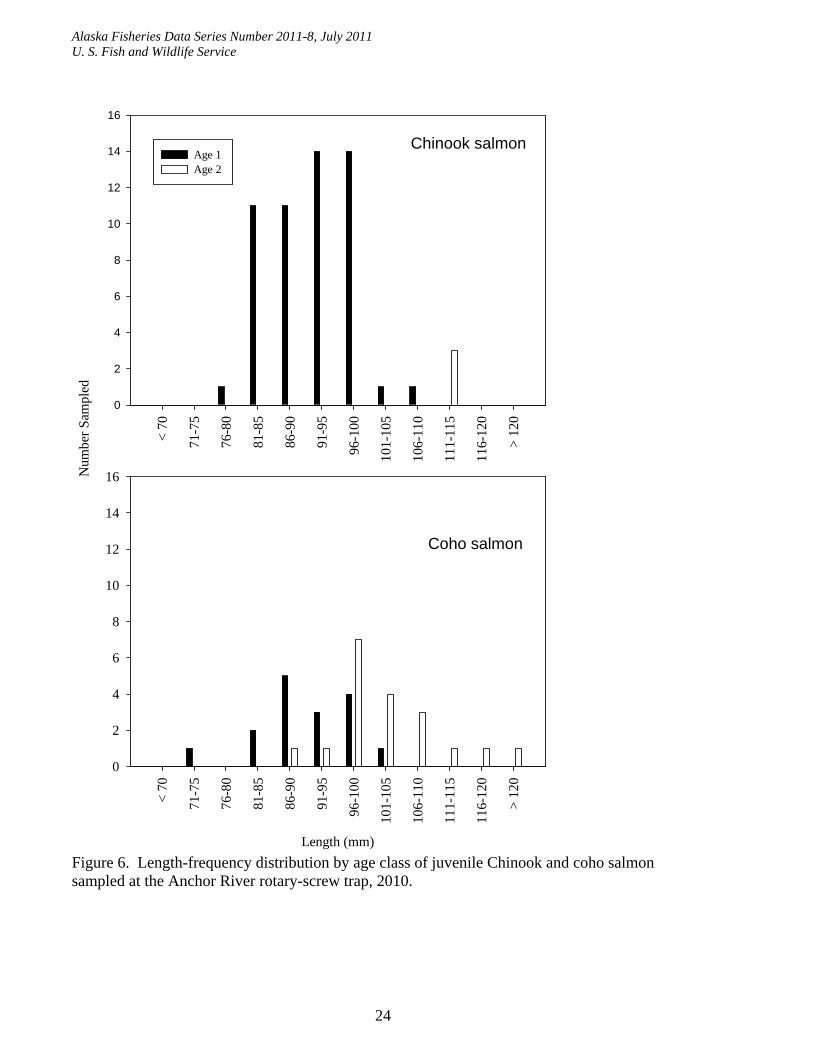
We only collected scale samples from n = 56 Chinook and n = 35 coho salmon smolts in 2010 and were unable to describe the weekly age composition for either species as per Objective 2. All but three Chinook salmon smolts sampled in 2010 were age 1, and age 2 smolts were larger than age 1 smolts (Figure 6). Most coho salmon longer than 95 mm were age 2 smolts and most less than 95 mm were age 1 (Figure 6). We did not collect scale samples from any Chinook or coho salmon smolts less than 70 mm in 2010, but few smolts that small were captured with the rotary-screw trap (Figures 4 and 5).
Juvenile Habitat Use
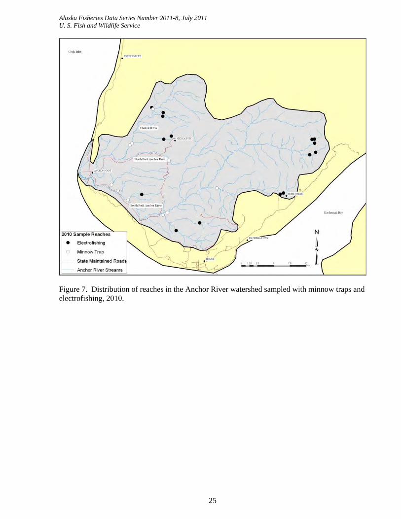
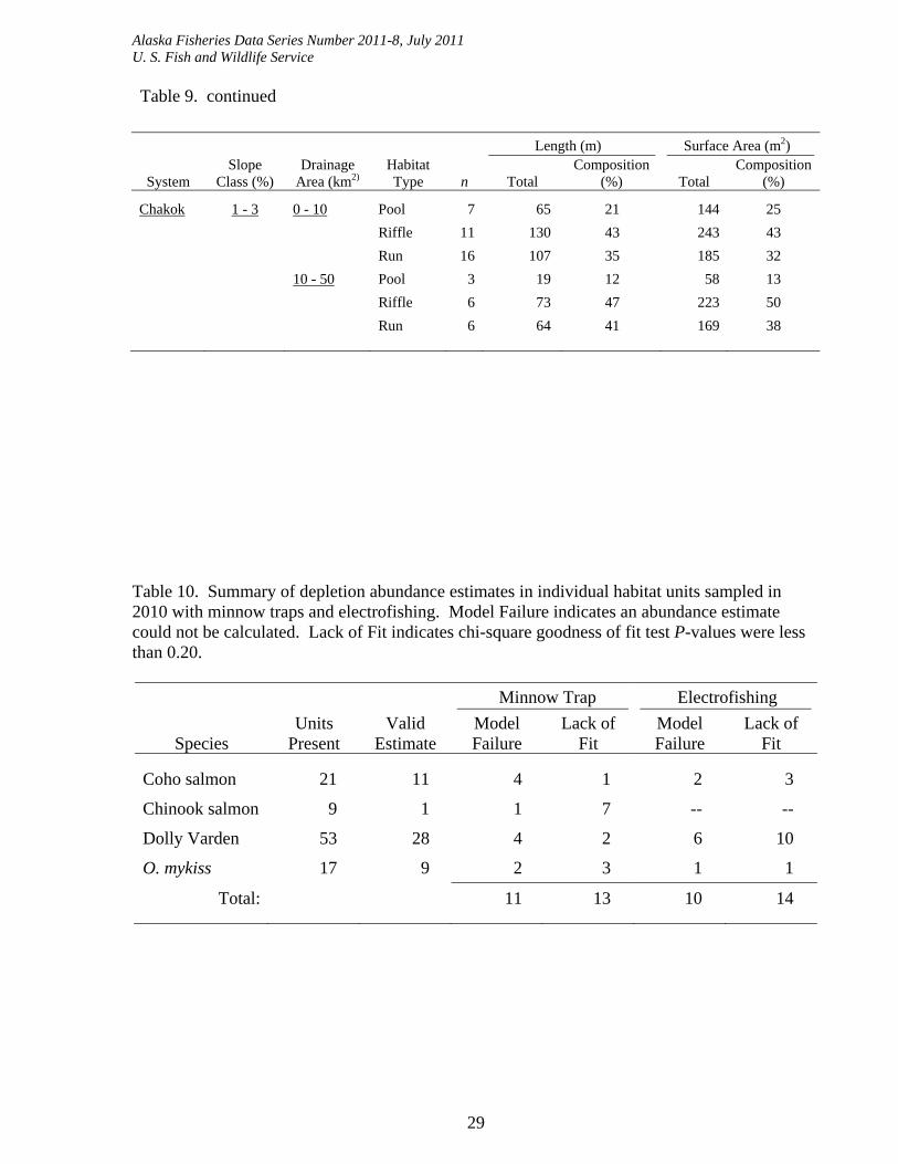
We sampled juvenile fish and habitat characteristics in 61 distinct habitat units in 25 reaches from 10 August to 24 September 2010; ten reaches were sampled with minnow traps and 15 were sampled using backpack electrofishing gear (Figure 7). Dolly Varden were the most widely distributed species and were observed in 53 of 61 habitat units; juvenile coho salmon were observed in 21 habitat units, juvenile Chinook salmon were observed in nine habitat units, and juvenile O. mykiss were observed in 17 habitat units (Tables 7 and 8). Dolly Varden was the only species present in 29 habitat units, and we did not capture any fish in five habitat units. Habitat composition data for our sampled reaches are summarized in Table 9.
Valid abundance estimates were only produced for about 50% of habitat units for coho salmon, Dolly Varden, and O. mykiss, but only one valid abundance estimate was produced for Chinook salmon (Table 10). Overall, most abundance estimate failures occurred when more fish were captured on the last capture occasion than on the previous pass. However, many estimates were rejected because chi-square goodness of fit test P-values were less than 0.20. Abundance estimate failures and model rejections due to lack of fit were equally likely among minnow trap and electrofishing depletion removal methods (Table 10).
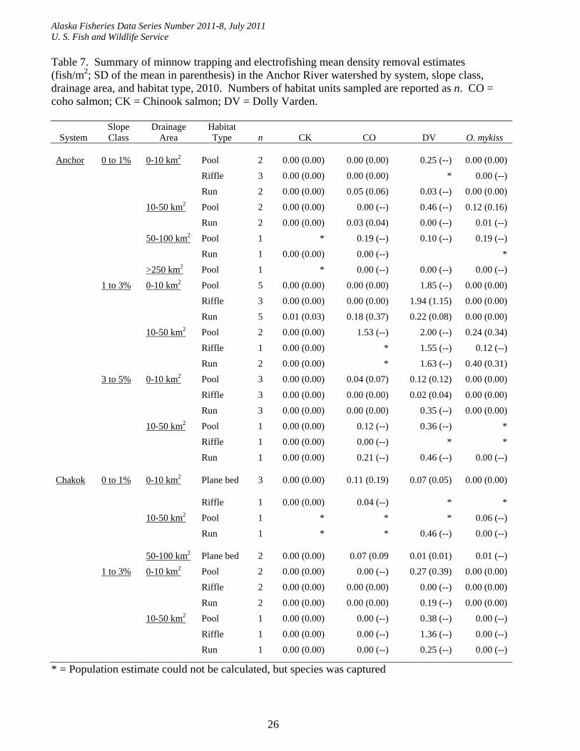
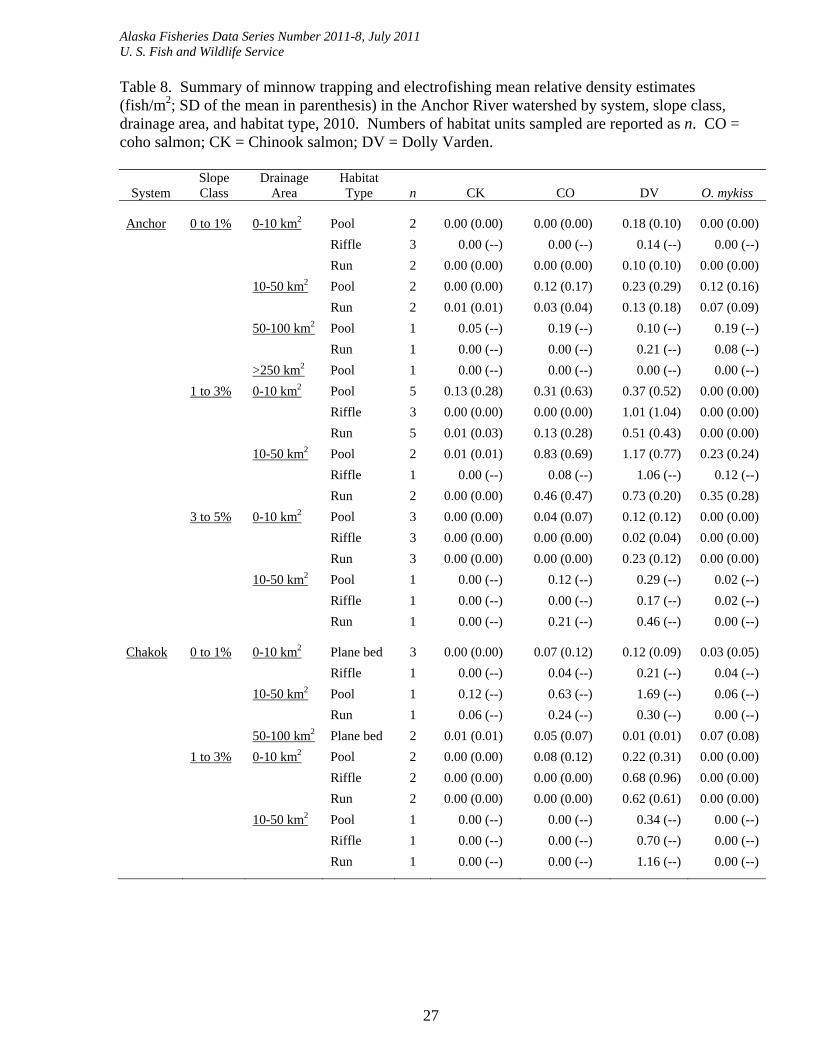
Mean densities (Table 7) and mean relative densities (Table 8) were generally low for Chinook salmon, coho salmon, and juvenile O. mykiss in most habitat types in 2010. Compared to the other species, mean densities and mean relative densities of Dolly Varden were generally greater in all areas we sampled (Tables 7 and 8).
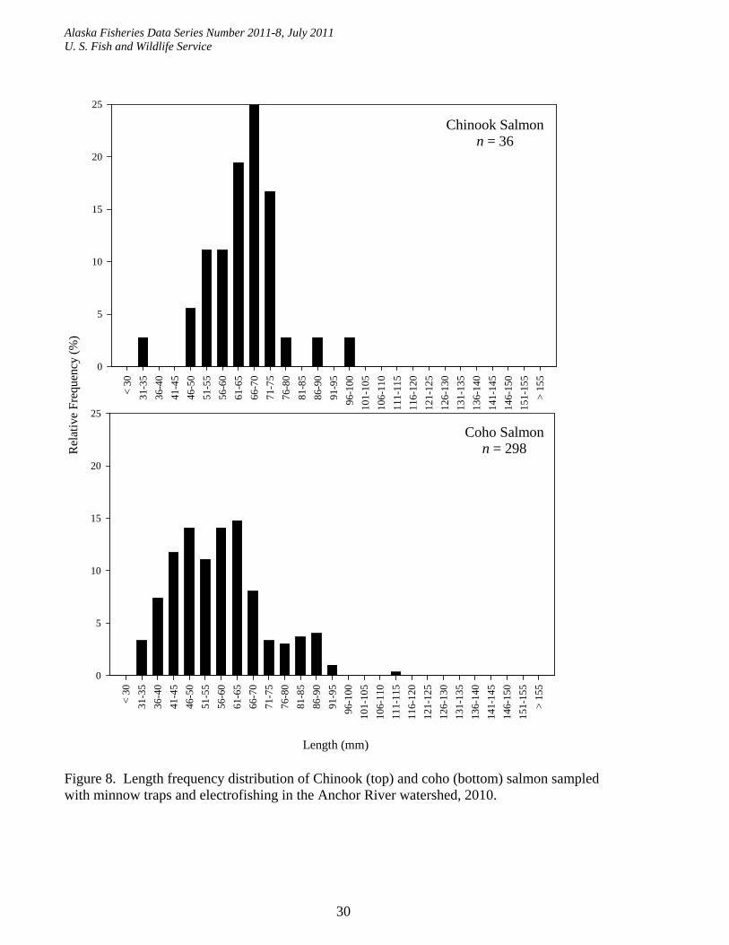
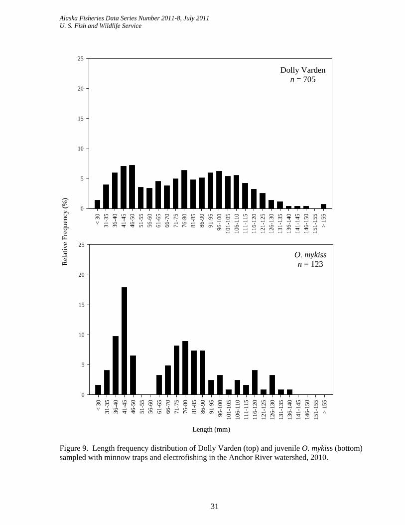
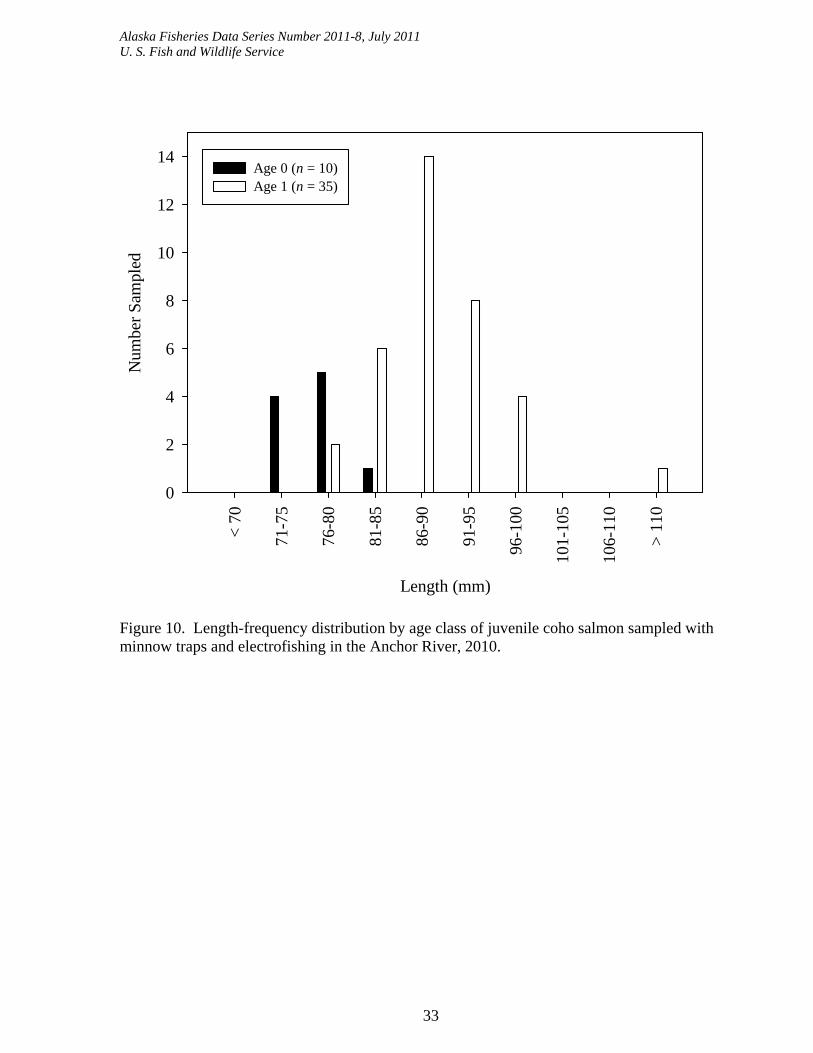
Lengths of juvenile Chinook salmon sampled in 2010 using minnow traps and electrofishing ranged from 31 to 96 mm although most were less than 75 mm; coho salmon lengths ranged from 32 to 113 mm and most were less than 70 mm (Figure 8). Dolly Varden sampled in 2010 ranged in length from 23 to 230 mm, and juvenile O. mykiss lengths ranged from 28 to 138 mm (Figure 9). The Dolly Varden and juvenile O. mykiss length-frequency distributions indicate we probably sampled at least three age classes in 2010.
Scales were collected from n = 45 coho salmon greater than 70 mm in length using minnow traps and electrofishing during August and September 2010. Most fish greater than 80 mm were
Alaska Fisheries Data Series Number 2011-8, July 2011 U. S. Fish and Wildlife Service
24
Chinook salmon<
70
71-7
5
76-8
0
81-8
5
86-9
0
91-9
5
96-1
00
101-
105
106-
110
111-
115
116-
120
> 1
20
0
2
4
6
8
10
12
14
16
Length (mm)
< 7
0
71-7
5
76-8
0
81-8
5
86-9
0
91-9
5
96-1
00
101-
105
106-
110
111-
115
116-
120
> 1
20
Num
ber
Sam
pled
0
2
4
6
8
10
12
14
16
Age 1 Age 2
Coho salmon
Figure 6. Length-frequency distribution by age class of juvenile Chinook and coho salmon sampled at the Anchor River rotary-screw trap, 2010.
Alaska Fisheries Data Series Number 2011-8, July 2011 U. S. Fish and Wildlife Service
25
Figure 7. Distribution of reaches in the Anchor River watershed sampled with minnow traps and electrofishing, 2010.
Alaska Fisheries Data Series Number 2011-8, July 2011 U. S. Fish and Wildlife Service
26
Table 7. Summary of minnow trapping and electrofishing mean density removal estimates (fish/m2; SD of the mean in parenthesis) in the Anchor River watershed by system, slope class, drainage area, and habitat type, 2010. Numbers of habitat units sampled are reported as n. CO = coho salmon; CK = Chinook salmon; DV = Dolly Varden.
System Slope Class
Drainage Area
Habitat Type n CK CO DV O. mykiss
Anchor 0 to 1% 0-10 km2 Pool 2 0.00 (0.00) 0.00 (0.00) 0.25 (--) 0.00 (0.00)
Riffle 3 0.00 (0.00) 0.00 (0.00) * 0.00 (--)
Run 2 0.00 (0.00) 0.05 (0.06) 0.03 (--) 0.00 (0.00)
10-50 km2 Pool 2 0.00 (0.00) 0.00 (--) 0.46 (--) 0.12 (0.16)
Run 2 0.00 (0.00) 0.03 (0.04) 0.00 (--) 0.01 (--)
50-100 km2 Pool 1 * 0.19 (--) 0.10 (--) 0.19 (--)
Run 1 0.00 (0.00) 0.00 (--) *
>250 km2 Pool 1 * 0.00 (--) 0.00 (--) 0.00 (--)
1 to 3% 0-10 km2 Pool 5 0.00 (0.00) 0.00 (0.00) 1.85 (--) 0.00 (0.00)
Riffle 3 0.00 (0.00) 0.00 (0.00) 1.94 (1.15) 0.00 (0.00)
Run 5 0.01 (0.03) 0.18 (0.37) 0.22 (0.08) 0.00 (0.00)
10-50 km2 Pool 2 0.00 (0.00) 1.53 (--) 2.00 (--) 0.24 (0.34)
Riffle 1 0.00 (0.00) * 1.55 (--) 0.12 (--)
Run 2 0.00 (0.00) * 1.63 (--) 0.40 (0.31)
3 to 5% 0-10 km2 Pool 3 0.00 (0.00) 0.04 (0.07) 0.12 (0.12) 0.00 (0.00)
Riffle 3 0.00 (0.00) 0.00 (0.00) 0.02 (0.04) 0.00 (0.00)
Run 3 0.00 (0.00) 0.00 (0.00) 0.35 (--) 0.00 (0.00)
10-50 km2 Pool 1 0.00 (0.00) 0.12 (--) 0.36 (--) *
Riffle 1 0.00 (0.00) 0.00 (--) * *
Run 1 0.00 (0.00) 0.21 (--) 0.46 (--) 0.00 (--)
Chakok 0 to 1% 0-10 km2 Plane bed 3 0.00 (0.00) 0.11 (0.19) 0.07 (0.05) 0.00 (0.00)
Riffle 1 0.00 (0.00) 0.04 (--) * *
10-50 km2 Pool 1 * * * 0.06 (--)
Run 1 * * 0.46 (--) 0.00 (--)
50-100 km2 Plane bed 2 0.00 (0.00) 0.07 (0.09 0.01 (0.01) 0.01 (--)
1 to 3% 0-10 km2 Pool 2 0.00 (0.00) 0.00 (--) 0.27 (0.39) 0.00 (0.00)
Riffle 2 0.00 (0.00) 0.00 (0.00) 0.00 (--) 0.00 (0.00)
Run 2 0.00 (0.00) 0.00 (0.00) 0.19 (--) 0.00 (0.00)
10-50 km2 Pool 1 0.00 (0.00) 0.00 (--) 0.38 (--) 0.00 (--)
Riffle 1 0.00 (0.00) 0.00 (--) 1.36 (--) 0.00 (--)
Run 1 0.00 (0.00) 0.00 (--) 0.25 (--) 0.00 (--)
* = Population estimate could not be calculated, but species was captured
Alaska Fisheries Data Series Number 2011-8, July 2011 U. S. Fish and Wildlife Service
27
Table 8. Summary of minnow trapping and electrofishing mean relative density estimates (fish/m2; SD of the mean in parenthesis) in the Anchor River watershed by system, slope class, drainage area, and habitat type, 2010. Numbers of habitat units sampled are reported as n. CO = coho salmon; CK = Chinook salmon; DV = Dolly Varden.
System Slope Class
Drainage Area
Habitat Type n CK CO DV O. mykiss
Anchor 0 to 1% 0-10 km2 Pool 2 0.00 (0.00) 0.00 (0.00) 0.18 (0.10) 0.00 (0.00)
Riffle 3 0.00 (--) 0.00 (--) 0.14 (--) 0.00 (--)
Run 2 0.00 (0.00) 0.00 (0.00) 0.10 (0.10) 0.00 (0.00)
10-50 km2 Pool 2 0.00 (0.00) 0.12 (0.17) 0.23 (0.29) 0.12 (0.16)
Run 2 0.01 (0.01) 0.03 (0.04) 0.13 (0.18) 0.07 (0.09)
50-100 km2 Pool 1 0.05 (--) 0.19 (--) 0.10 (--) 0.19 (--)
Run 1 0.00 (--) 0.00 (--) 0.21 (--) 0.08 (--)
>250 km2 Pool 1 0.00 (--) 0.00 (--) 0.00 (--) 0.00 (--)
1 to 3% 0-10 km2 Pool 5 0.13 (0.28) 0.31 (0.63) 0.37 (0.52) 0.00 (0.00)
Riffle 3 0.00 (0.00) 0.00 (0.00) 1.01 (1.04) 0.00 (0.00)
Run 5 0.01 (0.03) 0.13 (0.28) 0.51 (0.43) 0.00 (0.00)
10-50 km2 Pool 2 0.01 (0.01) 0.83 (0.69) 1.17 (0.77) 0.23 (0.24)
Riffle 1 0.00 (--) 0.08 (--) 1.06 (--) 0.12 (--)
Run 2 0.00 (0.00) 0.46 (0.47) 0.73 (0.20) 0.35 (0.28)
3 to 5% 0-10 km2 Pool 3 0.00 (0.00) 0.04 (0.07) 0.12 (0.12) 0.00 (0.00)
Riffle 3 0.00 (0.00) 0.00 (0.00) 0.02 (0.04) 0.00 (0.00)
Run 3 0.00 (0.00) 0.00 (0.00) 0.23 (0.12) 0.00 (0.00)
10-50 km2 Pool 1 0.00 (--) 0.12 (--) 0.29 (--) 0.02 (--)
Riffle 1 0.00 (--) 0.00 (--) 0.17 (--) 0.02 (--)
Run 1 0.00 (--) 0.21 (--) 0.46 (--) 0.00 (--)
Chakok 0 to 1% 0-10 km2 Plane bed 3 0.00 (0.00) 0.07 (0.12) 0.12 (0.09) 0.03 (0.05)
Riffle 1 0.00 (--) 0.04 (--) 0.21 (--) 0.04 (--)
10-50 km2 Pool 1 0.12 (--) 0.63 (--) 1.69 (--) 0.06 (--)
Run 1 0.06 (--) 0.24 (--) 0.30 (--) 0.00 (--)
50-100 km2 Plane bed 2 0.01 (0.01) 0.05 (0.07) 0.01 (0.01) 0.07 (0.08)
1 to 3% 0-10 km2 Pool 2 0.00 (0.00) 0.08 (0.12) 0.22 (0.31) 0.00 (0.00)
Riffle 2 0.00 (0.00) 0.00 (0.00) 0.68 (0.96) 0.00 (0.00)
Run 2 0.00 (0.00) 0.00 (0.00) 0.62 (0.61) 0.00 (0.00)
10-50 km2 Pool 1 0.00 (--) 0.00 (--) 0.34 (--) 0.00 (--)
Riffle 1 0.00 (--) 0.00 (--) 0.70 (--) 0.00 (--)
Run 1 0.00 (--) 0.00 (--) 1.16 (--) 0.00 (--)
Alaska Fisheries Data Series Number 2011-8, July 2011 U. S. Fish and Wildlife Service
28
Table 9. Summary of habitat composition sampling in the Anchor River watershed, 2010. Numbers of habitat units sampled are reported as n.
Length (m) Surface Area (m2)
System Slope
Class (%) Drainage
Area (km2) Habitat Type n Total
Composition (%) Total
Composition (%)
Anchor 0 - 1 0 - 10 Pool 8 74 25 202 30
Riffle 6 67 23 140 20
Run 7 157 53 343 50
10 - 50 Pool 11 179 42 963 45
Riffle 9 122 29 562 26
Run 8 127 30 603 28
50 - 100 Pool 4 66 35 268 40
Riffle 5 60 31 189 28
Run 4 63 33 209 31
>250 Pool 2 146 40 2,155 38
Riffle 2 148 41 2,508 45
Run 1 67 19 958 17
1 - 3 0 - 10 Plane bed 1 6 1 14 1
Pool 18 205 25 470 27
Riffle 25 323 40 709 40
Run 22 277 34 571 32
10 - 50 Pool 5 66 15 369 17
Riffle 14 276 65 1,379 65
Run 7 85 20 380 18
3 - 5 0 - 10 Pool 17 101 22 187 21
Riffle 19 193 42 365 42
Run 16 165 36 324 37
10 - 50 Pool 3 23 13 80 16
Riffle 5 115 66 342 67
Run 3 35 20 92 18
Chakok 0 - 1 0 - 10 Plane bed 8 232 80 442 76
Pool 1 6 2 15 3
Riffle 5 44 15 101 17
Run 1 8 3 25 4
10 - 50 Pool 6 74 36 311 36
Riffle 7 75 36 332 38
Run 3 58 28 220 26
50 - 100 Plane bed 9 301 58 1,793 58
Run 5 219 42 1,315 42
- continued -
Alaska Fisheries Data Series Number 2011-8, July 2011 U. S. Fish and Wildlife Service
29
Table 9. continued
Length (m) Surface Area (m2)
System Slope
Class (%) Drainage
Area (km2) Habitat Type n Total
Composition (%) Total
Composition (%)
Chakok 1 - 3 0 - 10 Pool 7 65 21 144 25
Riffle 11 130 43 243 43
Run 16 107 35 185 32
10 - 50 Pool 3 19 12 58 13
Riffle 6 73 47 223 50
Run 6 64 41 169 38
Table 10. Summary of depletion abundance estimates in individual habitat units sampled in 2010 with minnow traps and electrofishing. Model Failure indicates an abundance estimate could not be calculated. Lack of Fit indicates chi-square goodness of fit test P-values were less than 0.20.
Minnow Trap Electrofishing
Species Units
Present Valid
Estimate Model Failure
Lack of Fit
Model Failure
Lack of Fit
Coho salmon 21 11 4 1 2 3
Chinook salmon 9 1 1 7 -- --
Dolly Varden 53 28 4 2 6 10
O. mykiss 17 9 2 3 1 1
Total: 11 13 10 14
Alaska Fisheries Data Series Number 2011-8, July 2011 U. S. Fish and Wildlife Service
30
Coho Salmonn = 298
< 3
0
31-3
5
36-4
0
41-4
5
46-5
0
51-5
5
56-6
0
61-6
5
66-7
0
71-7
5
76-8
0
81-8
5
86-9
0
91-9
5
96-1
00
101-
105
106-
110
111-
115
116-
120
121-
125
126-
130
131-
135
136-
140
141-
145
146-
150
151-
155
> 1
55
Rel
ativ
e F
requ
ency
(%
)
0
5
10
15
20
25
Chinook Salmonn = 36
Length (mm)
< 3
0
31-3
5
36-4
0
41-4
5
46-5
0
51-5
5
56-6
0
61-6
5
66-7
0
71-7
5
76-8
0
81-8
5
86-9
0
91-9
5
96-1
00
101-
105
106-
110
111-
115
116-
120
121-
125
126-
130
131-
135
136-
140
141-
145
146-
150
151-
155
> 1
55
0
5
10
15
20
25
Figure 8. Length frequency distribution of Chinook (top) and coho (bottom) salmon sampled with minnow traps and electrofishing in the Anchor River watershed, 2010.
Alaska Fisheries Data Series Number 2011-8, July 2011 U. S. Fish and Wildlife Service
31
Dolly Vardenn = 705
< 3
0
31-3
5
36-4
0
41-4
5
46-5
0
51-5
5
56-6
0
61-6
5
66-7
0
71-7
5
76-8
0
81-8
5
86-9
0
91-9
5
96-1
00
101-
105
106-
110
111-
115
116-
120
121-
125
126-
130
131-
135
136-
140
141-
145
146-
150
151-
155
> 1
55
Rel
ativ
e Fr
eque
ncy
(%)
0
5
10
15
20
25
O. mykissn = 123
Length (mm)
< 3
0
31-3
5
36-4
0
41-4
5
46-5
0
51-5
5
56-6
0
61-6
5
66-7
0
71-7
5
76-8
0
81-8
5
86-9
0
91-9
5
96-1
00
101-
105
106-
110
111-
115
116-
120
121-
125
126-
130
131-
135
136-
140
141-
145
146-
150
151-
155
> 1
55
0
5
10
15
20
25
Figure 9. Length frequency distribution of Dolly Varden (top) and juvenile O. mykiss (bottom) sampled with minnow traps and electrofishing in the Anchor River watershed, 2010.
Alaska Fisheries Data Series Number 2011-8, July 2011 U. S. Fish and Wildlife Service
32
age 1, while most fish less than 80 mm were age 0 (Figure 10). We did not collect scale samples from any fish less than 70 mm, but assume most fish less than 70 mm were age 0. Based on this assumption, most juvenile coho salmon sampled in 2010 (Figure 8) were age 0. Adult Escapement
We operated the ADF&G weir on the Anchor River beginning on 1 August and used underwater video to monitor passage beginning on the afternoon of 2 August until the weir was pulled on 28 September. We counted n = 5,973 coho salmon passing the weir in August and September (Appendix C) and a total escapement of N = 6,014 included n = 41 fish that passed the weir in July (Carol Kerkvliet, ADF&G, personal communication). We counted n = 581 steelhead passing through the weir in August and September for a total count of n = 593 which included n = 12 fish that passed the weir in July (Carol Kerkvliet, ADF&G, personal communication). Other species observed at the Anchor River weir in August and September included Chinook (n = 184), chum (n = 53), pink (n = 936), and sockeye (n = 201) salmon, and Dolly Varden (n = 1,232).
Peaks in coho salmon passage corresponded with high flow freshets (Figure 11) and 90% of passage occurred prior to 5 September (Appendix C). Most steelhead passage occurred on the descending hydrograph throughout most of September and steelhead were still observed passing the weir when it was pulled on 28 September. Therefore, we did not count a portion of the steelhead run that entered the Anchor River after the weir was pulled. Steelhead passage occurred almost exclusively at night between 21:00 and 04:00 hours, but we did not observe a similar trend for coho salmon (Figure 12).
A summary of daily water temperatures is presented in Appendix D, and a summary of mean daily stage height compared to historical data is presented in Appendix E.
Discussion
We were successful in operating a rotary-screw trap on the Anchor River during 2010 to estimate Chinook and coho salmon smolt abundance and migration timing. However, we were not able to safely operate the trap because of high river velocities early in the season and were therefore not able to monitor the entire Chinook salmon smolt outmigration. We also had to stop fishing the screw trap on three occasions during high flow events when velocities exceeded safe operating levels. Our options for trap placement were limited and we did not have the ability to move the trap to other areas to avoid high flows. We were limited based on our sampling needs to locations downstream of the confluence of the North and South forks where smolts from both streams had a chance to mix. We were also limited by fisheries concerns to keep the trap within the 90-m reach downstream of the weir that was closed to fishing to avoid conflicts with sport anglers. We are limited to the same trap location in 2011, and our sampling success may again be influenced by high flow conditions.
Since we missed the beginning of the Chinook salmon smolt outmigration and had to pull the cone on three occasions for a total of 48 hours during the sampling season, our estimates of smolt abundance are therefore minimum estimates because of these gaps in data collection. We had limited success modeling missing data because there were no consistent environmental parameters or other parameters that were related to capture efficiencies, smolt numbers, or passage rates (CPUE) for Chinook and coho salmon. Also, all three high water events that prevented us from fishing the trap occurred during overnight periods, which was also the peak
Alaska Fisheries Data Series Number 2011-8, July 2011 U. S. Fish and Wildlife Service
33
Length (mm)
< 7
0
71-7
5
76-8
0
81-8
5
86-9
0
91-9
5
96-1
00
101-
105
106-
110
> 1
10
Num
ber
Sam
pled
0
2
4
6
8
10
12
14Age 0 (n = 10)Age 1 (n = 35)
Figure 10. Length-frequency distribution by age class of juvenile coho salmon sampled with minnow traps and electrofishing in the Anchor River, 2010.
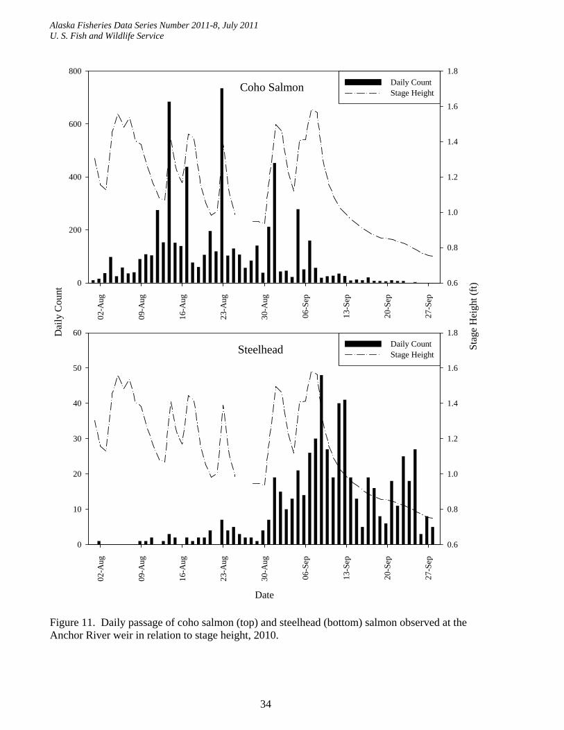
Alaska Fisheries Data Series Number 2011-8, July 2011 U. S. Fish and Wildlife Service
34
Coho Salmon02
-Aug
09-A
ug
16-A
ug
23-A
ug
30-A
ug
06-S
ep
13-S
ep
20-S
ep
27-S
ep
Dai
ly C
ount
0
200
400
600
800
Sta
ge H
eigh
t (ft
)0.6
0.8
1.0
1.2
1.4
1.6
1.8Daily CountStage Height
Steelhead
Date
02-A
ug
09-A
ug
16-A
ug
23-A
ug
30-A
ug
06-S
ep
13-S
ep
20-S
ep
27-S
ep
0
10
20
30
40
50
60
0.6
0.8
1.0
1.2
1.4
1.6
1.8Daily CountStage Height
Figure 11. Daily passage of coho salmon (top) and steelhead (bottom) salmon observed at the Anchor River weir in relation to stage height, 2010.
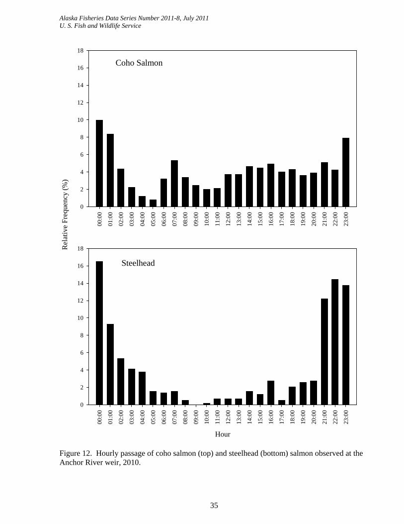
Alaska Fisheries Data Series Number 2011-8, July 2011 U. S. Fish and Wildlife Service
35
Coho Salmon
00:0
0
01:0
0
02:0
0
03:0
0
04:0
0
05:0
0
06:0
0
07:0
0
08:0
0
09:0
0
10:0
0
11:0
0
12:0
0
13:0
0
14:0
0
15:0
0
16:0
0
17:0
0
18:0
0
19:0
0
20:0
0
21:0
0
22:0
0
23:0
0
Rel
ativ
e F
requ
ency
(%
)
0
2
4
6
8
10
12
14
16
18
Steelhead
Hour
00:0
0
01:0
0
02:0
0
03:0
0
04:0
0
05:0
0
06:0
0
07:0
0
08:0
0
09:0
0
10:0
0
11:0
0
12:0
0
13:0
0
14:0
0
15:0
0
16:0
0
17:0
0
18:0
0
19:0
0
20:0
0
21:0
0
22:0
0
23:0
0
0
2
4
6
8
10
12
14
16
18
Figure 12. Hourly passage of coho salmon (top) and steelhead (bottom) salmon observed at the Anchor River weir, 2010.
Alaska Fisheries Data Series Number 2011-8, July 2011 U. S. Fish and Wildlife Service
36
movement period for smolts. We could have modeled missing data using weak relationships between cone RPM and daily capture efficiencies for coho salmon (r2 = 0.04; P = 0.041) and between cone RPM and smolt numbers for Chinook salmon (r2 = 0.07; P = 0.011), but RPM data were not available when the cone was pulled, and modeling would have required extrapolating outside of the range of observed values during the three occasions of missing data. We believe this was not appropriate and would have added more uncertainty to our estimates. We are still investigating other approaches to model the missing data including simple linear interpolation, fitting of run timing curves, stepwise regression, and modeling data over shorter time periods surrounding each occasion of missing data, but did not want this aspect of the data analysis to prevent timely reporting of 2010 results.
Missing data must be modeled prior to analysis of Objective 4 because any smolts missed in the 2010 abundance estimate will result in bias for the smolt-to-spawning adult survival estimate. For example, if smolt abundance in 2010 is underestimated, survival will be biased upward. We will also use the missing data as a sensitivity analysis for the estimate of smolt-to-spawning adult survival by presenting survival with and without interpolation of missing smolt abundance data, which may indicate how robust our survival estimate is to missing smolt abundance data points.
Because of difficulties identifying a suitable location for a release live well, we were unable to estimate short-term mark survival in each stratum as recommended by Carlson et al. (1998) as described in the Methods section. We planned to hold a sample of 25 marked and 25 unmarked smolts in a live well for at least 1 day in each tagging strata and count remaining marked and unmarked live fish. The estimated mark survival would have provided us with a coarse estimate of handling mortality. We initially spent time identifying a suitable location, but were unable to construct a second live well and conduct the experiment after we experienced the mortality event while attempting to relocate the live well. We will estimate short-term mark survival during 2011, and results will provide some insight into probable handling mortalities experienced during 2010. However, our observed mortality for marked fish held in the live well each day prior to an evening release indicates we had relatively low (< 1%) short-term mortality for our marked fish (n = 22 Chinook salmon and n = 12 coho salmon).
Most mark-recapture assumptions for an unbiased Lincoln-Petersen estimate of smolt abundance following Carlson et al. (1998) were met for most strata. These assumptions included: 1) closed population; 2) all smolts have the same probability of being marked or all smolts have the same probability of being examined for marks; 3) constant capture probability; 4) marks are not lost between release and recovery; 5) all marked smolts are reported; and 6) all marked smolts released are either recovered or pass by the downstream capture site. Assumption 1 was probably met in most strata, and mortality observed during handling and marking was minimal (<1%) and was censored from the estimate. Our trap was not size selective and our release site at the confluence of the North and South forks allowed marked fish to mix with the general smolt population prior to recapture (Assumption 2). The partial caudal fin-clips used as marks were clearly visible to the crew when recaptured at the screw trap and did not regenerate in the short time period between release and recovery (Assumption 4). The crew was properly trained in fish handling and marking techniques and followed procedures to ensure all captured fish were examined for marks and all marks were reported (Assumption 5). We only marked and released fish classified as smolt or transitional, and 98% of marked smolts migrated past the screw trap during the same strata of release (Assumption 6).
Alaska Fisheries Data Series Number 2011-8, July 2011 U. S. Fish and Wildlife Service
37
Although fish were marked and released daily, it may not be appropriate to investigate relationships using daily capture efficiencies because not all marked fish moved past the screw trap immediately after release; therefore, the number of fish available for capture upstream of the trap on any given day may have been greater than the number recently released. Most marked smolts migrated past the smolt trap shortly after release, but some fish were recaptured in a different stratum than released. Because of the relative low numbers of smolts (n = 52 Chinook salmon and n = 28 coho salmon) exhibiting this behavior, we assume any bias associated with Assumption 6 is minimal because 98% of all marked smolts passed the capture site within their tagging stratum. Thedinga et al (1994) also noted most recaptures occurred shortly after release: 2-28% within one day and 90% within one week of release. Unique daily marks would allow for more detailed analysis and modeling of capture efficiencies and allow us to track fates of daily releases with more detail (Roper and Scarnecchia 2000), but is not practical with batch marks. Uniquely-numbered tags such as passive-integrated transponder tags might be practical, but they are not feasible for this project based on our goal to minimize fish handling and because of available funding.
Assumption 3 requires capture efficiency to be constant within each stratum. Many factors can influence trap efficiency including time of release and turbidity (Eskelin 2004), changing stream flow conditions (Volkhardt et al. 2007), fish size and species (Thedinga et al. 1994; Volkhardt et al. 2007), and changes to how the trap is operated (e.g., moved to different positions, addition of screen panels). To address these factors, we used the same release site and released fish at or near dusk each day, we developed separate estimates for Chinook and coho salmon, we tested for size selectivity, and we did not change the screw trap location or operating pattern once we started fishing on 3 June. However, we did not measure turbidity, and we were not able to develop predictive relationships between changing flow conditions and different measures of smolt capture (capture efficiency, smolt numbers, CPUE).
Capture efficiencies for Chinook and coho salmon were not constant over the course of the sampling season (Tables 5 and 6) and G-tests of independence (Sokal and Rohlf 1981) indicate capture efficiency data were not independent of tagging strata and should not be pooled (P < 0.0001 for both species). Since we used batch marks and not all fish were recaptured the day after release, we were unable to calculate true daily capture efficiencies and are therefore unable to test whether capture efficiencies were constant within each tagging stratum. Variable capture efficiencies within tagging strata can lead to bias, although Carlson et al. (1998) found minimal bias even though true capture efficiencies varied considerably within their sampling strata (e.g., from 10% to 35% in two of their five sampling periods). They recommend minimizing stratum length while maintaining discrete sampling periods, and found that periods of about one week were appropriate. Volkhardt et al. (2007) also recommend strata durations between three days and one week.
Our observed numbers and mean densities of juvenile Chinook and coho salmon were low throughout the Anchor River in 2010 (Tables 7 and 8). In general, coho salmon and juvenile O. mykiss relative densities were higher in habitat units sampled in the 1-3% slope class in the Anchor River and in the 0-1% slope class in the Chakok River, while Dolly Varden were more prevalent in habitat units in the 1-3% slope class in both systems (Tables 7 and 8). We did not observe many juvenile Chinook salmon in 2010, but we did not sample many habitat units in larger streams (drainage area > 50 km2). These larger habitat units may provide better rearing habitat since juvenile Chinook salmon are typically found in larger main channel, high-velocity areas compared to coho salmon (Murphy et al. 1989; Healey 1991). Also, most Chinook salmon
Alaska Fisheries Data Series Number 2011-8, July 2011 U. S. Fish and Wildlife Service
38
spawning likely occurs in the mainstem Anchor River below where most of our juvenile sampling occurred in 2010.
Mean densities of juvenile coho salmon were low in most habitat units in the Anchor River watershed compared to other areas in the Pacific Northwest. Mean coho salmon relative density in pool habitats across all systems, slope classes, and drainage areas was only 0.22 fish/m2 in 2010. This value is well below densities used to model habitat limiting factors in Oregon streams (mean summer densities > 1.5 fish/m2 in pool habitat; Nickelson 1998) and well below levels believed to represent fully seeded habitat for juvenile coho salmon in the Pacific Northwest (1.0 fish/m2 in pools; Nickelson et al. 1992). Anderson and Hetrick (2004) also observed mean summer densities of juvenile coho salmon in pool habitats greater than 1.4 fish/m2 during one year of their study in streams on the Alaska Peninsula, although they observed lower densities (0.43 fish/m2) during the second year of monitoring. They attributed the lower densities during the second year of sampling to a low spawning escapement of adult coho salmon the previous year. Observed coho salmon escapement in the Anchor River during 2009 was only 2,691 fish, the lowest recorded since monitoring began in 2004 (Table 1), which may be below levels necessary to fully seed habitat in the Anchor River watershed. A larger spawning escapement of adult coho salmon as occurred in 2010 would likely lead to a more wide-spread distribution of adults to some of the areas where we did not observe juvenile fish in 2010, and would also likely lead to higher juvenile densities observed the following summer. Sampling in 2011 may provide further support of these observations.
Our inability to obtain accurate abundance estimates of juvenile coho salmon based on removal experiments in many habitat units (Table 10) was probably due to several factors. For all experiments, initial abundance of juvenile coho salmon may have been too small to allow for effective sampling as White et al. (1982) suggest population sizes of at least 200 individuals are needed for reliable estimates. Model failures or cases of lack of model fit where chi-square goodness of fit test P-values were greater than 0.20 (White et al. 1982) did not appear to be related to gear type (Table 10), and usually occurred when more fish were captured on the last capture occasion than on the previous pass. It is likely that behavior and movement patterns of juvenile salmonids played some role in our inability to achieve depletion. Our block nets appeared to be functioning (allowing no immigration or emigration), minnow traps were set in the same places for each capture event, equal effort was expended during each electrofishing pass, and there were no areas where fish were congregated or observed in schools between capture events. There may have been some localized areas of cover present where fish could have avoided capture by hiding between capture events, and in some habitat units it appeared that fish were displaced during the first electrofishing pass which resulted in higher capture numbers during the second pass. However, this does not explain catching more fish on the final pass. We may have been successful in obtaining reliable abundance estimates by conducting a greater number of removal events, but in many cases it was not practical to do so. For 2011, our protocol will include additional passes if depletion was not observed on the final pass.

Alaska Fisheries Data Series Number 2011-8, July 2011 U. S. Fish and Wildlife Service
39
Recommendations
Following our field work and analysis of 2010 data, we recommend the following to improve sampling to achieve objectives during the 2011 field season:
1. Monitor turbidity at the screw trap as an environmental parameter that may help model smolt movement.
2. Estimate short-term survival of fin-clipped Chinook and coho salmon as described in the Methods. We did not do this in 2010.
3. For all depletion estimates, add extra passes if more fish are captured on the last pass than on the previous pass.
4. Collect scale samples from the requisite sample sizes of Chinook and coho salmon smolts at the screw trap (n = 11 of each species). We did not achieve sample size goals in 2010 and were therefore unable to achieve Objective 2.
5. Collect scale samples from all juvenile coho salmon greater than 60 mm during electrofishing/minnow trap sampling instead of 70 mm to verify lower length range of age 1 parr.
6. Sample larger stream sizes to better describe juvenile Chinook salmon habitat use in the Anchor River watershed.
Acknowledgements
We thank USFWS crew members W. Atwood, M. Banner, and K. Perkins, and ADF&G crew members A. Pollak and G. Chiraboga for their efforts throughout the field season. We also thank USFWS personnel J. Boersma and K. Gates for their technical assistance over the course of the field season. N. Szarzi, C. Kerkvliet, and M. Booz with ADF&G assisted with planning, logistics, and project implementation. We thank the staff at ADF&G for providing the rotary-screw trap and M. Hatfield for his assistance getting the trap functioning properly. Finally, we thank the numerous landowners who allowed us access to their property during the course of this project.
Alaska Fisheries Data Series Number 2011-8, July 2011 U. S. Fish and Wildlife Service
40
References
Anderson, J. L., and N. J. Hetrick. 2004. Carrying capacity of habitats used seasonally by coho salmon in the Kametolook River, Alaska Peninsula National Wildlife Refuge, 2002-2003. U. S. Fish and Wildlife Service, King Salmon Fish and Wildlife Field Office, Alaska Fisheries Technical Report Number 73, King Salmon, Alaska.
Anderson, J. L., N. J. Hetrick, D. Spencer, J. P. Larson, and M. Santos. 2006. Design and performance of a digital video monitoring system incorporated in a V-shaped resistance board weir. U.S. Fish and Wildlife Service, King Salmon Fish and Wildlife Field Office, Alaska Fisheries Technical Report Number 91, King Salmon, Alaska.
Bisson, P. A., J. L. Nielsen, R. A. Palmason, and L. E. Groves. 1982. A system of naming habitat types in small streams with examples of habitat utilization by salmonids during low streamflow. Pages 62-73 in N. B. Armantrout, editor. Acquisition and utilization of aquatic habitat inventory information. Proceedings of a symposium held 28-30 October, 1981, Western Division of the American Fisheries Society, Portland, Oregon.
Bromaghin, J. F. 1993. Sample size determination for interval estimation of multinomial probabilities. The American Statistician 47:203-206.
Bryant, M. D. 2000. Estimating fish populations by removal methods with minnow traps in Southeast Alaska streams. North American Journal of Fisheries Management 20:923-930.
Bryant, M. D. 2009. Global climate change and potential effects on Pacific salmonids in freshwater ecosystems of southeast Alaska. Climatic Change 95:169-193.
Carlson, S. R., L. G. Coggins Jr., and C. O. Swanton. 1998. A simple stratified design for mark-recapture estimation of salmon smolt abundance. Alaska Fishery Research Bulletin 5:88-102.
CBFWA (Columbia Basin Fish and Wildlife Authority). 1999. PIT tag marking procedures manual, version 2.0. PIT tag Steering Committee, Portland, Oregon.
Dalbey, S. R., T. E. McMahon, and W. Fredenberg. 1996. Effect of electrofishing pulse shape and electrofishing-induced spinal injury on long-term growth and survival of wild rainbow trout. North American Journal of Fisheries Management 16:560-569.
Downs, C. C., D. Horan, E. Morgan-Harris, and R. Jakubowski. 2006. Spawning demographics and juvenile dispersal of an adfluvial bull trout population in Trestle Creek, Idaho. North American Journal of Fisheries Management 26:190–200.
Eskelin, A. A. 2004. An assessment of trap efficiency to estimate coho salmon smolt abundance in a small Alaskan stream. Master’s Thesis, University of Alaska-Fairbanks, Fairbanks, Alaska.
Ewing, R. D., M. D. Evenson, E. K. Birks, and A. R. Hemmingsen. 1984. Indices of parr-smolt transformation in juvenile steelhead trout (Salmo gairdneri) undergoing volitional release at Cole Rivers Hatchery, Oregon. Aquaculture 40:209-221.
Feyrer, F., T. Sommer, and W. Harrell. 2006. Importance of flood dynamics versus intrinsic physical habitat in structuring fish communities: evidence from two adjacent engineered floodplains on the Sacramento River, California. North American Journal of Fisheries Management 26:408–417.
Alaska Fisheries Data Series Number 2011-8, July 2011 U. S. Fish and Wildlife Service
41
Gates, K. S., and J. K. Boersma. 2009. Abundance and run timing of adult steelhead in Crooked and Nikolai creeks, Kenai Peninsula, Alaska, 2008. U.S. Fish and Wildlife Service, Kenai Fish and Wildlife Field Office, Alaska Fisheries Data Series Number 2009-2, Soldotna, Alaska.
Hankin, D. G. 1984. Multistage sampling designs in fisheries research: applications in small streams. Canadian Journal of Fisheries and Aquatic Sciences 41:1575-1591.
Hankin, D. G., and G. H. Reeves. 1988. Estimating total fish abundance and total habitat area in small streams based on visual estimation methods. Canadian Journal of Fisheries and Aquatic Sciences 45:834-844.
Healey, M. C. 1991. Life history of Chinook salmon (Oncorhynchus tshawytscha). Pages 311-393 in C. Groot and L. Margolis, editors. Pacific salmon life histories. University of British Columbia Press, Vancouver, British Columbia.
Jearld, A. 1983. Age determination. Pages 301 - 324 in L. A. Nielsen and D. L. Johnson, editors. Fisheries Techniques. American Fisheries Society, Bethesda, Maryland.
Johnson, J., and K. Klein. 2009. Catalog of waters important for spawning, rearing, or migration of anadromous fishes – Southcentral Region, Effective June 1, 2009. Alaska Department of Fish and Game, Special Publication No. 09-03, Anchorage, Alaska.
Kennen, J. G., S. J. Wisniewski, and N. H. Ringler. 1994. Application and modification of an auger trap to quantify emigrating fishes in Lake Ontario tributaries. North American Journal of Fisheries Management 14:828–836.
Kerkvliet, C. M., D. L. Burwen, and R. N. Begich. 2008. Anchor River 2003 and 2004 Chinook salmon and 2004 coho salmon escapement. Alaska Department of Fish and Game, Fishery Data Series No. 08-06, Anchorage, Alaska.
Kyle, R. E., and T. P. Brabets. 2001. Water temperature of streams in the Cook Inlet Basin, Alaska, and implications of climate change. U. S. Geological Survey, Water-Resources Investigations Report 01-4109, Anchorage, Alaska.
Mauger, S. 2005. Lower Kenai Peninsula’s salmon streams: annual water quality assessment, July 2004 – September 2005. Cook Inletkeeper, Homer, Alaska.
Mauger, S. 2008. Action steps toward greater protection of lower Kenai Peninsula’s salmon streams, July 2007 – June 2008. Cook Inletkeeper, Homer, Alaska.
Miller, B. A., and S. Sadro. 2003. Residence time and seasonal movements of juvenile coho salmon in the ecotone and lower estuary of Winchester Creek, South Slough, Oregon. Transactions of the American Fisheries Society 132:546–559.
Mobrand, L. E., J. A. Lichatowich, L. C. Lestelle, and T. S. Vogel. 1997. An approach to describing ecosystem performance “through the eyes of salmon”. Canadian Journal of Fisheries and Aquatic Sciences 54:2964-2973.
Montgomery, D. R., and J. M. Buffington. 1997. Channel-reach morphology in mountain drainage basins. Geological Society of America Bulletin 109:596-611.
Mosher, K. H. 1968. Photographic atlas of sockeye salmon scales. Fishery Bulletin 67:243-280.
Alaska Fisheries Data Series Number 2011-8, July 2011 U. S. Fish and Wildlife Service
42
Murphy, M. L., J. Heifetz, J. F. Thedinga, S. W. Johnson, and K. V. Koski. 1989. Habitat utilization by juvenile Pacific salmon in the glacial Taku River, Southeast Alaska. Canadian Journal of Fisheries and Aquatic Sciences 46:1677-1685.
Nickelson, T. E. 1998. A habitat-based assessment of coho salmon production potential and spawner escapement needs for Oregon coastal streams. Oregon Department of Fish and Wildlife Information Reports Number 98-4, Portland, Oregon.
Nickelson, T. E., Rodgers, J. D., S. L. Johnson, and M. F. Solazzi. 1992. Seasonal changes in habitat use by juvenile coho salmon (Oncorhynchus kisutch) in Oregon coastal streams. Canadian Journal of Fisheries and Aquatic Sciences 49:783-789.
Overton, C. K., S. P. Wollrab, B. C. Roberts, and M. A. Radko. 1997. R1/R4 (Northern/Intermountain Regions) fish and fish habitat standard inventory procedures handbook. USDA Forest Service, General Technical Report INT-GTR-346, Ogden, Utah.
Pollard, W. R., G. F. Hartman, C. Groot, and P. Edgell. 1997. Field identification of coastal juvenile salmonids. Harbour Publishing, Madeira Park, British Columbia.
Pollock, K. H., and M. C. Otto. 1983. Robust estimation of population size in closed animal populations from capture-recapture experiments. Biometrics 39:1035-1049.
Pollock, K. H., J. D. Nichols, C. Brownie, and J. E. Hines. 1990. Statistical inference for capture-recapture experiments. Wildlife Monographs 107:1-97.
Reynolds, J. B. 1996. Electrofishing. Pages 221 – 253 in B. R. Murphy and D. W. Willis, editors. Fisheries techniques, 2nd edition. American Fisheries Society, Bethesda, Maryland.
Reynolds, L., A. T. Herlihy, P. R. Kaufmann, S. V. Gregory, and R. M. Hughes. 2003. Electrofishing effort requirements for assessing species richness and biotic integrity in western Oregon streams. North American Journal of Fisheries Management 23:450-461.
Richter, A., and S. A. Kolmes. 2005. Maximum temperature limits for Chinook, coho, and chum salmon, and steelhead trout in the Pacific Northwest. Reviews in Fisheries Science 13:23-49.
Riley, S. C., and K. D. Fausch. 1992. Underestimation of trout population size by maximum-likelihood removal estimates in small streams. North American Journal of Fisheries Management 12:768-776.
Roper, B. B., and D. L. Scarnecchia. 1996. A comparison of wild and hatchery-reared age-0 Chinook salmon trap efficiencies. North American Journal of Fisheries Management 16:214-217.
Roper, B. B., and D. L. Scarnecchia. 1999. Emigration of age-0 Chinook salmon (Oncorhynchus tshawytscha) smolts from the upper South Umpqua River basin, Oregon, U.S.A. Canadian Journal of Fisheries and Aquatic Sciences 56:939-946.
Roper, B. B., and D. L. Scarnecchia. 2000. Key strategies for estimating population sizes of emigrating salmon smolts with a single trap. Rivers 7:77-88.
Ross, D. W., G. E. Daterman, J. L. Boughton, and T. M. Quigley. 2001. Forest health restoration in south-central Alaska: a problem analysis. USDA Forest Service, General Technical Report PNW-GTR-523, Portland, Oregon.
Alaska Fisheries Data Series Number 2011-8, July 2011 U. S. Fish and Wildlife Service
43
Sandercock, F. K. 1991. Life history of coho salmon (Oncorhynchus kisutch). Pages 395-446 in C. Groot and L. Margolis, editors. Pacific salmon life histories. University of British Columbia Press, Vancouver, British Columbia.
Schoettger, R. A., and A. M. Julin. 1967. Efficacy of MS-222 as an anesthetic on four salmonids. United States Bureau of Sports Fisheries and Wildlife Investigations in Fish Control No 13, Washington, D. C.
Seber, G. A. F. 1982. The estimation of animal abundance and related parameters, second edition. Macmillan, New York.
Seelbach, P. W., R. N. Lockwood, and G. R. Alexander. 1985. A modified incline-screen trap for catching salmon in large rivers. North American Journal of Fisheries Management 5:494-498.
Sokal, R. R., and F. J. Rohlf. 1981. Biometry, second edition. W. H. Freeman and Company, New York, New York.
Steinhorst, K., Y. Wu, B. Dennis, and P. Kline. 2004. Confidence intervals for fish out-migration estimates using stratified trap efficiency methods. Journal of Agricultural, Biological, and Environmental Statistics 9:284-299.
Stillwater Sciences. 2009. RIPPLE case study: coho salmon enhancement, Rock Creek, Oregon. Stillwater Sciences, Arcata, California.
Strahler, A. N. 1952. Dynamic basis of geomorphology. Geological Society of America Bulletin 63:923-938.
Sykes, G. E., C. J. Johnson, and J. M. Shrimpton. 2009. Temperature and flow effects on migration timing of Chinook salmon smolts. Transactions of the American Fisheries Society 138:1252–1265.
Szarzi, N. J., C. M. Kerkvliet, C. E. Stock, and M. D. Booz. 2007. Recreational fisheries in the Lower Cook Inlet Management Area, 2005-2007, with updates for 2004. Alaska Department of Fish and Game, Fishery Management Report No. 07-55, Anchorage, Alaska.
Thedinga, J. F., M. L. Murphy, S. W. Johnson, J. M. Lorenz, and K. V. Koski. 1994. Determination of salmonid smolt yield with rotary-screw traps in the Situk River, Alaska, to predict effects of glacial flooding. North American Journal of Fisheries Management 14:837-851.
USFWS (U. S. Fish and Wildlife Service). 2004. Electrofishing. Chapter 6, part 241. Safety operations, occupational safety and health. USFWS, Washington, D.C.
Venditti, D., A. Kohler, C. Bretz, N. Brindza, J. Lockhart, A. Brimmer, and K. Apperson. 2006. Idaho Supplementation Studies; Brood Year 2003 Cooperative Report. 2003-2005 Progress Report for Project No. 198909800 (et al.), BPA Report DOE/BP-00006630-6, Portland, Oregon.
Viola, A. E., and M. L. Shuck. 1995. A method to reduce the abundance of residual hatchery steelhead in rivers. North American Journal of Fisheries Management 15:488-493.
Volkhardt, G. C., S. L. Johnson, B. A. Miller, T. E. Nickelson, and D. E. Seiler. 2007. Rotary screw traps and inclined plane screen traps. Pages 235-266 in D. H. Johnson, B. M. Shrier, J. S. O’Neal, J. A. Knutzen, X Augerot, T. A. O’Neil, and T. N. Pearsons. Salmonid field protocols handbook: techniques for assessing status and trends in salmon and trout populations. American Fisheries Society, Bethesda, Maryland.
Alaska Fisheries Data Series Number 2011-8, July 2011 U. S. Fish and Wildlife Service
44
Walker, C., R. King, D. Whigham, and S. Baird. 2007. Wetland geomorphic linkages to juvenile salmonids and macroinvertebrate communities in headwater streams of the Kenai Lowlands, Alaska. U.S. EPA Region 10 Wetland Program Development Program, Final Report.
Walker, C., R. King, M. C. Rains, D. Whigham, S. Baird, and J. Bellino. 2009. Headwater stream wetland settings and shallow ground water influence: relationships to juvenile salmon habitat on the Kenai Peninsula, Alaska. U.S. EPA Region 10 Wetland Program Development Program Final Report.
Wedemeyer, G. A., R. L. Saunders, and W. C. Clarke. 1980. Environmental factors affecting smoltification and early marine survival of anadromous salmonids. Marine Fisheries Review 42:1-14.
White, G. C., D. R. Anderson, K. P. Burnham, and D. L. Otis. 1982. Capture-recapture and removal methods for sampling closed populations. Los Alamos National Laboratory, Los Alamos, New Mexico.
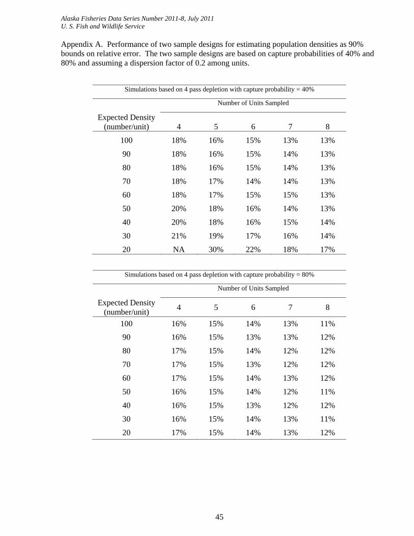
Alaska Fisheries Data Series Number 2011-8, July 2011 U. S. Fish and Wildlife Service
45
Appendix A. Performance of two sample designs for estimating population densities as 90% bounds on relative error. The two sample designs are based on capture probabilities of 40% and 80% and assuming a dispersion factor of 0.2 among units.
Simulations based on 4 pass depletion with capture probability = 40%
Number of Units Sampled
Expected Density (number/unit) 4 5 6 7 8
100 18% 16% 15% 13% 13%
90 18% 16% 15% 14% 13%
80 18% 16% 15% 14% 13%
70 18% 17% 14% 14% 13%
60 18% 17% 15% 15% 13%
50 20% 18% 16% 14% 13%
40 20% 18% 16% 15% 14%
30 21% 19% 17% 16% 14%
20 NA 30% 22% 18% 17%
Simulations based on 4 pass depletion with capture probability = 80%
Number of Units Sampled
Expected Density (number/unit)
4 5 6 7 8
100 16% 15% 14% 13% 11%
90 16% 15% 13% 13% 12%
80 17% 15% 14% 12% 12%
70 17% 15% 13% 12% 12%
60 17% 15% 14% 13% 12%
50 16% 15% 14% 12% 11%
40 16% 15% 13% 12% 12%
30 16% 15% 14% 13% 11%
20 17% 15% 14% 13% 12%
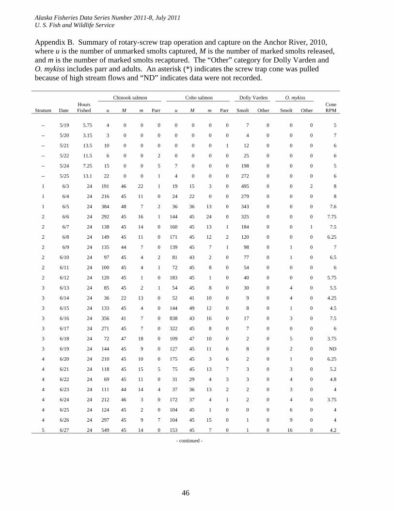
Alaska Fisheries Data Series Number 2011-8, July 2011 U. S. Fish and Wildlife Service
46
Appendix B. Summary of rotary-screw trap operation and capture on the Anchor River, 2010, where u is the number of unmarked smolts captured, M is the number of marked smolts released, and m is the number of marked smolts recaptured. The “Other” category for Dolly Varden and O. mykiss includes parr and adults. An asterisk (*) indicates the screw trap cone was pulled because of high stream flows and “ND” indicates data were not recorded.
Chinook salmon Coho salmon Dolly Varden O. mykiss
Stratum Date Hours Fished u M m Parr u M m Parr Smolt Other Smolt Other
Cone RPM
-- 5/19 5.75 4 0 0 0 0 0 0 0 7 0 0 0 5
-- 5/20 3.15 3 0 0 0 0 0 0 0 4 0 0 0 7
-- 5/21 13.5 10 0 0 0 0 0 0 1 12 0 0 0 6
-- 5/22 11.5 6 0 0 2 0 0 0 0 25 0 0 0 6
-- 5/24 7.25 15 0 0 5 7 0 0 0 198 0 0 0 5
-- 5/25 13.1 22 0 0 1 4 0 0 0 272 0 0 0 6
1 6/3 24 191 46 22 1 19 15 3 0 495 0 0 2 8
1 6/4 24 216 45 11 0 24 22 0 0 279 0 0 0 8
1 6/5 24 384 48 7 2 36 36 13 0 343 0 0 0 7.6
2 6/6 24 292 45 16 1 144 45 24 0 325 0 0 0 7.75
2 6/7 24 138 45 14 0 160 45 13 1 184 0 0 1 7.5
2 6/8 24 149 45 11 0 171 45 12 2 120 0 0 0 6.25
2 6/9 24 135 44 7 0 139 45 7 1 98 0 1 0 7
2 6/10 24 97 45 4 2 81 43 2 0 77 0 1 0 6.5
2 6/11 24 100 45 4 1 72 45 8 0 54 0 0 0 6
2 6/12 24 120 45 1 0 183 45 1 0 40 0 0 0 5.75
3 6/13 24 85 45 2 1 54 45 8 0 30 0 4 0 5.5
3 6/14 24 36 22 13 0 52 41 10 0 9 0 4 0 4.25
3 6/15 24 133 45 4 0 144 49 12 0 8 0 1 0 4.5
3 6/16 24 356 41 7 0 838 43 16 0 17 0 3 0 7.5
3 6/17 24 271 45 7 0 322 45 8 0 7 0 0 0 6
3 6/18 24 72 47 18 0 109 47 10 0 2 0 5 0 3.75
3 6/19 24 144 45 9 0 127 45 11 6 8 0 2 0 ND
4 6/20 24 210 45 10 0 175 45 3 6 2 0 1 0 6.25
4 6/21 24 118 45 15 5 75 45 13 7 3 0 3 0 5.2
4 6/22 24 69 45 11 0 31 29 4 3 3 0 4 0 4.8
4 6/23 24 111 44 14 4 37 36 13 2 2 0 3 0 4
4 6/24 24 212 46 3 0 172 37 4 1 2 0 4 0 3.75
4 6/25 24 124 45 2 0 104 45 1 0 0 0 6 0 4
4 6/26 24 297 45 9 7 104 45 15 0 1 0 9 0 4
5 6/27 24 549 45 14 0 153 45 7 0 1 0 16 0 4.2
- continued -
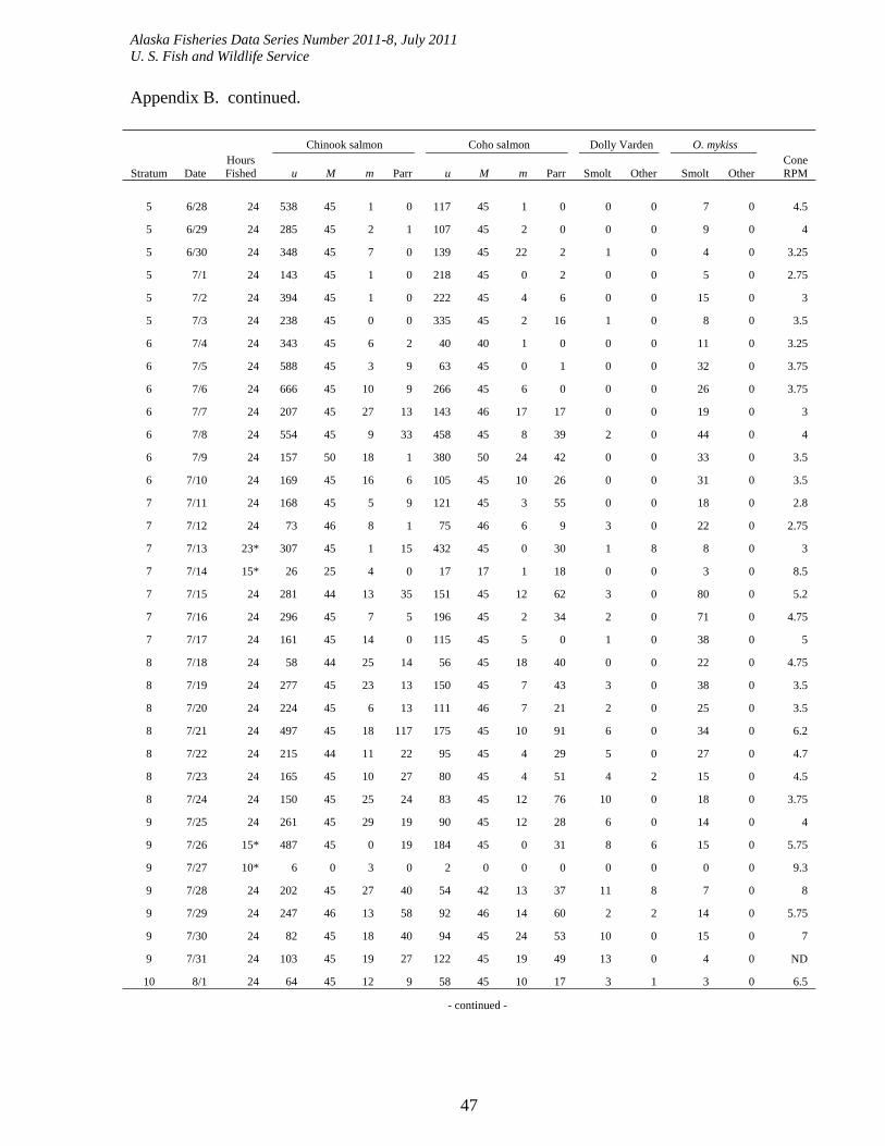
Alaska Fisheries Data Series Number 2011-8, July 2011 U. S. Fish and Wildlife Service
47
Appendix B. continued.
Chinook salmon Coho salmon Dolly Varden O. mykiss
Stratum Date Hours Fished u M m Parr u M m Parr Smolt Other Smolt Other
Cone RPM
5 6/28 24 538 45 1 0 117 45 1 0 0 0 7 0 4.5
5 6/29 24 285 45 2 1 107 45 2 0 0 0 9 0 4
5 6/30 24 348 45 7 0 139 45 22 2 1 0 4 0 3.25
5 7/1 24 143 45 1 0 218 45 0 2 0 0 5 0 2.75
5 7/2 24 394 45 1 0 222 45 4 6 0 0 15 0 3
5 7/3 24 238 45 0 0 335 45 2 16 1 0 8 0 3.5
6 7/4 24 343 45 6 2 40 40 1 0 0 0 11 0 3.25
6 7/5 24 588 45 3 9 63 45 0 1 0 0 32 0 3.75
6 7/6 24 666 45 10 9 266 45 6 0 0 0 26 0 3.75
6 7/7 24 207 45 27 13 143 46 17 17 0 0 19 0 3
6 7/8 24 554 45 9 33 458 45 8 39 2 0 44 0 4
6 7/9 24 157 50 18 1 380 50 24 42 0 0 33 0 3.5
6 7/10 24 169 45 16 6 105 45 10 26 0 0 31 0 3.5
7 7/11 24 168 45 5 9 121 45 3 55 0 0 18 0 2.8
7 7/12 24 73 46 8 1 75 46 6 9 3 0 22 0 2.75
7 7/13 23* 307 45 1 15 432 45 0 30 1 8 8 0 3
7 7/14 15* 26 25 4 0 17 17 1 18 0 0 3 0 8.5
7 7/15 24 281 44 13 35 151 45 12 62 3 0 80 0 5.2
7 7/16 24 296 45 7 5 196 45 2 34 2 0 71 0 4.75
7 7/17 24 161 45 14 0 115 45 5 0 1 0 38 0 5
8 7/18 24 58 44 25 14 56 45 18 40 0 0 22 0 4.75
8 7/19 24 277 45 23 13 150 45 7 43 3 0 38 0 3.5
8 7/20 24 224 45 6 13 111 46 7 21 2 0 25 0 3.5
8 7/21 24 497 45 18 117 175 45 10 91 6 0 34 0 6.2
8 7/22 24 215 44 11 22 95 45 4 29 5 0 27 0 4.7
8 7/23 24 165 45 10 27 80 45 4 51 4 2 15 0 4.5
8 7/24 24 150 45 25 24 83 45 12 76 10 0 18 0 3.75
9 7/25 24 261 45 29 19 90 45 12 28 6 0 14 0 4
9 7/26 15* 487 45 0 19 184 45 0 31 8 6 15 0 5.75
9 7/27 10* 6 0 3 0 2 0 0 0 0 0 0 0 9.3
9 7/28 24 202 45 27 40 54 42 13 37 11 8 7 0 8
9 7/29 24 247 46 13 58 92 46 14 60 2 2 14 0 5.75
9 7/30 24 82 45 18 40 94 45 24 53 10 0 15 0 7
9 7/31 24 103 45 19 27 122 45 19 49 13 0 4 0 ND
10 8/1 24 64 45 12 9 58 45 10 17 3 1 3 0 6.5
- continued -
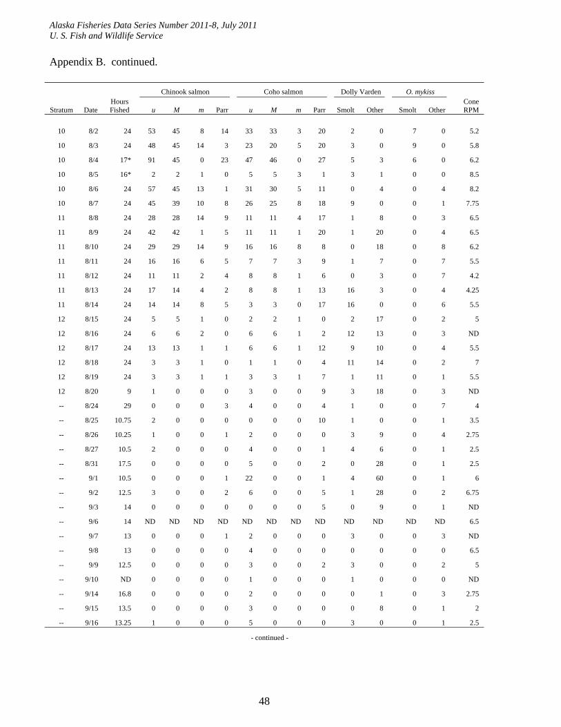
Alaska Fisheries Data Series Number 2011-8, July 2011 U. S. Fish and Wildlife Service
48
Appendix B. continued.
Chinook salmon Coho salmon Dolly Varden O. mykiss
Stratum Date Hours Fished u M m Parr u M m Parr Smolt Other Smolt Other
Cone RPM
10 8/2 24 53 45 8 14 33 33 3 20 2 0 7 0 5.2
10 8/3 24 48 45 14 3 23 20 5 20 3 0 9 0 5.8
10 8/4 17* 91 45 0 23 47 46 0 27 5 3 6 0 6.2
10 8/5 16* 2 2 1 0 5 5 3 1 3 1 0 0 8.5
10 8/6 24 57 45 13 1 31 30 5 11 0 4 0 4 8.2
10 8/7 24 45 39 10 8 26 25 8 18 9 0 0 1 7.75
11 8/8 24 28 28 14 9 11 11 4 17 1 8 0 3 6.5
11 8/9 24 42 42 1 5 11 11 1 20 1 20 0 4 6.5
11 8/10 24 29 29 14 9 16 16 8 8 0 18 0 8 6.2
11 8/11 24 16 16 6 5 7 7 3 9 1 7 0 7 5.5
11 8/12 24 11 11 2 4 8 8 1 6 0 3 0 7 4.2
11 8/13 24 17 14 4 2 8 8 1 13 16 3 0 4 4.25
11 8/14 24 14 14 8 5 3 3 0 17 16 0 0 6 5.5
12 8/15 24 5 5 1 0 2 2 1 0 2 17 0 2 5
12 8/16 24 6 6 2 0 6 6 1 2 12 13 0 3 ND
12 8/17 24 13 13 1 1 6 6 1 12 9 10 0 4 5.5
12 8/18 24 3 3 1 0 1 1 0 4 11 14 0 2 7
12 8/19 24 3 3 1 1 3 3 1 7 1 11 0 1 5.5
12 8/20 9 1 0 0 0 3 0 0 9 3 18 0 3 ND
-- 8/24 29 0 0 0 3 4 0 0 4 1 0 0 7 4
-- 8/25 10.75 2 0 0 0 0 0 0 10 1 0 0 1 3.5
-- 8/26 10.25 1 0 0 1 2 0 0 0 3 9 0 4 2.75
-- 8/27 10.5 2 0 0 0 4 0 0 1 4 6 0 1 2.5
-- 8/31 17.5 0 0 0 0 5 0 0 2 0 28 0 1 2.5
-- 9/1 10.5 0 0 0 1 22 0 0 1 4 60 0 1 6
-- 9/2 12.5 3 0 0 2 6 0 0 5 1 28 0 2 6.75
-- 9/3 14 0 0 0 0 0 0 0 5 0 9 0 1 ND
-- 9/6 14 ND ND ND ND ND ND ND ND ND ND ND ND 6.5
-- 9/7 13 0 0 0 1 2 0 0 0 3 0 0 3 ND
-- 9/8 13 0 0 0 0 4 0 0 0 0 0 0 0 6.5
-- 9/9 12.5 0 0 0 0 3 0 0 2 3 0 0 2 5
-- 9/10 ND 0 0 0 0 1 0 0 0 1 0 0 0 ND
-- 9/14 16.8 0 0 0 0 2 0 0 0 0 1 0 3 2.75
-- 9/15 13.5 0 0 0 0 3 0 0 0 0 8 0 1 2
-- 9/16 13.25 1 0 0 0 5 0 0 0 3 0 0 1 2.5
- continued -
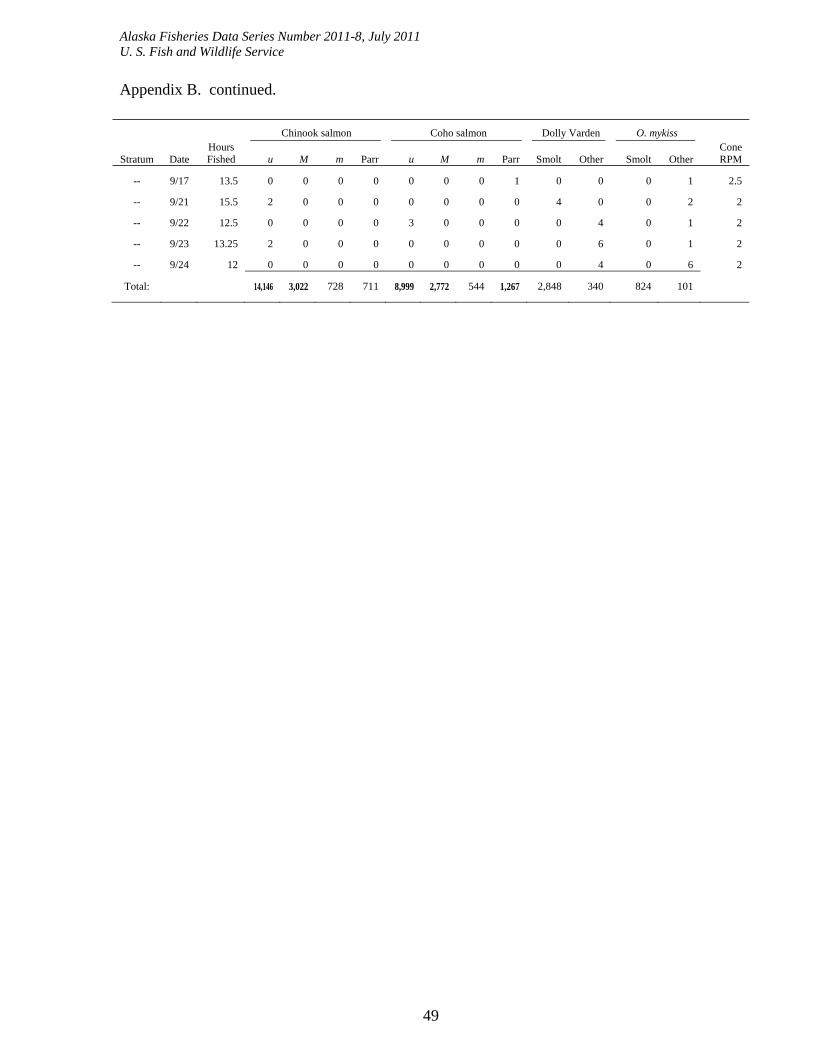
Alaska Fisheries Data Series Number 2011-8, July 2011 U. S. Fish and Wildlife Service
49
Appendix B. continued.
Chinook salmon Coho salmon Dolly Varden O. mykiss
Stratum Date Hours Fished u M m Parr u M m Parr Smolt Other Smolt Other
Cone RPM
-- 9/17 13.5 0 0 0 0 0 0 0 1 0 0 0 1 2.5
-- 9/21 15.5 2 0 0 0 0 0 0 0 4 0 0 2 2
-- 9/22 12.5 0 0 0 0 3 0 0 0 0 4 0 1 2
-- 9/23 13.25 2 0 0 0 0 0 0 0 0 6 0 1 2
-- 9/24 12 0 0 0 0 0 0 0 0 0 4 0 6 2
Total: 14,146 3,022 728 711 8,999 2,772 544 1,267 2,848 340 824 101
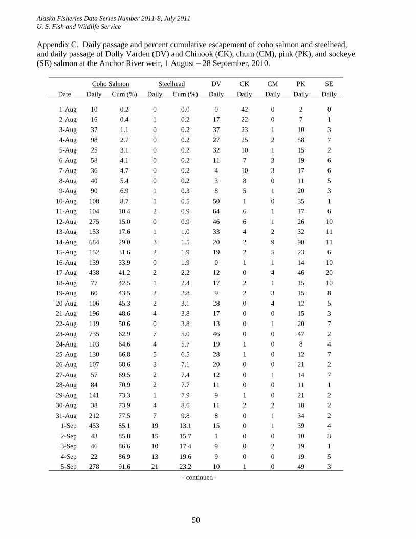
Alaska Fisheries Data Series Number 2011-8, July 2011 U. S. Fish and Wildlife Service
50
Appendix C. Daily passage and percent cumulative escapement of coho salmon and steelhead, and daily passage of Dolly Varden (DV) and Chinook (CK), chum (CM), pink (PK), and sockeye (SE) salmon at the Anchor River weir, 1 August – 28 September, 2010.
Coho Salmon Steelhead DV CK CM PK SE
Date Daily Cum (%) Daily Cum (%) Daily Daily Daily Daily Daily
1-Aug 10 0.2 0 0.0 0 42 0 2 0
2-Aug 16 0.4 1 0.2 17 22 0 7 1
3-Aug 37 1.1 0 0.2 37 23 1 10 3
4-Aug 98 2.7 0 0.2 27 25 2 58 7
5-Aug 25 3.1 0 0.2 32 10 1 15 2
6-Aug 58 4.1 0 0.2 11 7 3 19 6
7-Aug 36 4.7 0 0.2 4 10 3 17 6
8-Aug 40 5.4 0 0.2 3 8 0 11 5
9-Aug 90 6.9 1 0.3 8 5 1 20 3
10-Aug 108 8.7 1 0.5 50 1 0 35 1
11-Aug 104 10.4 2 0.9 64 6 1 17 6
12-Aug 275 15.0 0 0.9 46 6 1 26 10
13-Aug 153 17.6 1 1.0 33 4 2 32 11
14-Aug 684 29.0 3 1.5 20 2 9 90 11
15-Aug 152 31.6 2 1.9 19 2 5 23 6
16-Aug 139 33.9 0 1.9 0 1 1 14 10
17-Aug 438 41.2 2 2.2 12 0 4 46 20
18-Aug 77 42.5 1 2.4 17 2 1 15 10
19-Aug 60 43.5 2 2.8 9 2 3 15 8
20-Aug 106 45.3 2 3.1 28 0 4 12 5
21-Aug 196 48.6 4 3.8 17 0 0 15 3
22-Aug 119 50.6 0 3.8 13 0 1 20 7
23-Aug 735 62.9 7 5.0 46 0 0 47 2
24-Aug 103 64.6 4 5.7 19 1 0 8 4
25-Aug 130 66.8 5 6.5 28 1 0 12 7
26-Aug 107 68.6 3 7.1 20 0 0 21 2
27-Aug 57 69.5 2 7.4 12 0 1 14 7
28-Aug 84 70.9 2 7.7 11 0 0 11 1
29-Aug 141 73.3 1 7.9 9 1 0 21 2
30-Aug 38 73.9 4 8.6 11 2 2 18 2
31-Aug 212 77.5 7 9.8 8 0 1 34 2
1-Sep 453 85.1 19 13.1 15 0 1 39 4
2-Sep 43 85.8 15 15.7 1 0 0 10 3
3-Sep 46 86.6 10 17.4 9 0 2 19 1
4-Sep 22 86.9 13 19.6 9 0 0 19 5
5-Sep 278 91.6 21 23.2 10 1 0 49 3
- continued -
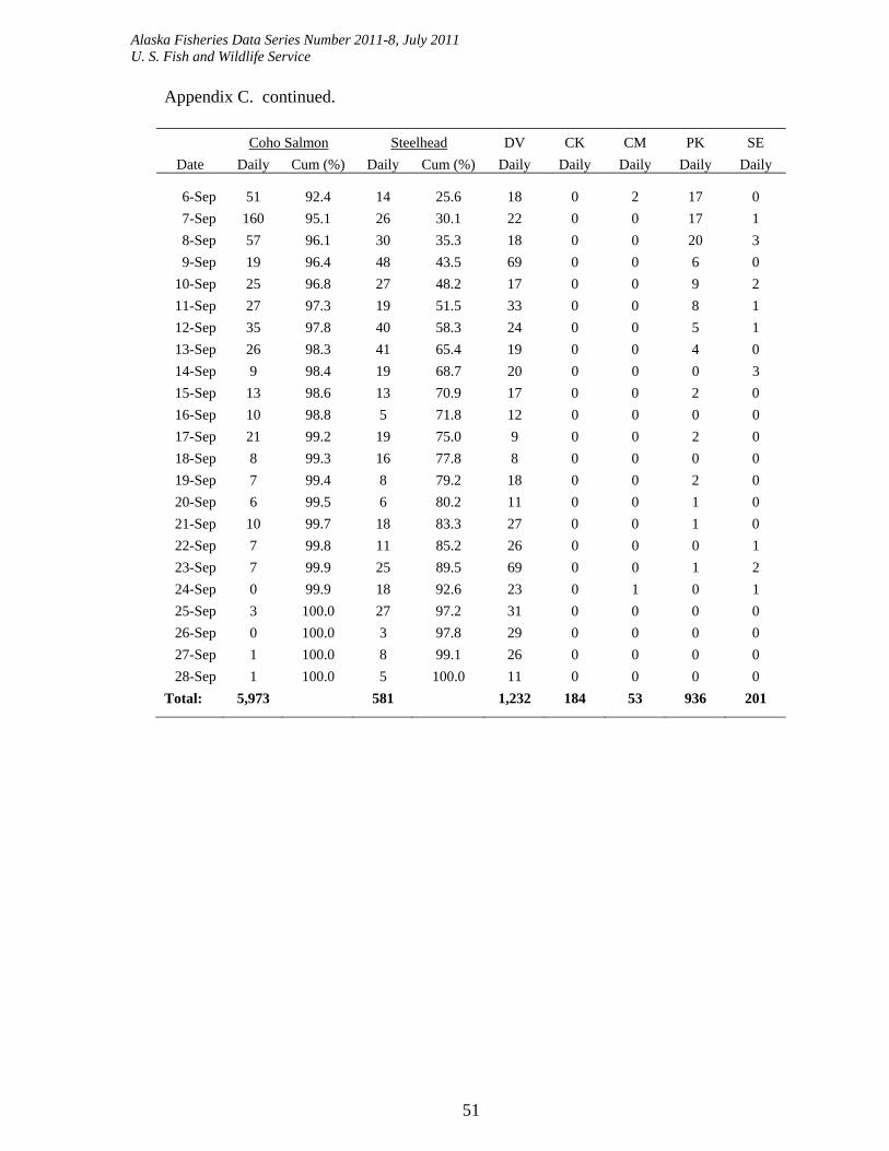
Alaska Fisheries Data Series Number 2011-8, July 2011 U. S. Fish and Wildlife Service
51
Appendix C. continued.
Coho Salmon Steelhead DV CK CM PK SE
Date Daily Cum (%) Daily Cum (%) Daily Daily Daily Daily Daily
6-Sep 51 92.4 14 25.6 18 0 2 17 0
7-Sep 160 95.1 26 30.1 22 0 0 17 1
8-Sep 57 96.1 30 35.3 18 0 0 20 3
9-Sep 19 96.4 48 43.5 69 0 0 6 0
10-Sep 25 96.8 27 48.2 17 0 0 9 2
11-Sep 27 97.3 19 51.5 33 0 0 8 1
12-Sep 35 97.8 40 58.3 24 0 0 5 1
13-Sep 26 98.3 41 65.4 19 0 0 4 0
14-Sep 9 98.4 19 68.7 20 0 0 0 3
15-Sep 13 98.6 13 70.9 17 0 0 2 0
16-Sep 10 98.8 5 71.8 12 0 0 0 0
17-Sep 21 99.2 19 75.0 9 0 0 2 0
18-Sep 8 99.3 16 77.8 8 0 0 0 0
19-Sep 7 99.4 8 79.2 18 0 0 2 0
20-Sep 6 99.5 6 80.2 11 0 0 1 0
21-Sep 10 99.7 18 83.3 27 0 0 1 0
22-Sep 7 99.8 11 85.2 26 0 0 0 1
23-Sep 7 99.9 25 89.5 69 0 0 1 2
24-Sep 0 99.9 18 92.6 23 0 1 0 1
25-Sep 3 100.0 27 97.2 31 0 0 0 0
26-Sep 0 100.0 3 97.8 29 0 0 0 0
27-Sep 1 100.0 8 99.1 26 0 0 0 0
28-Sep 1 100.0 5 100.0 11 0 0 0 0
Total: 5,973 581 1,232 184 53 936 201
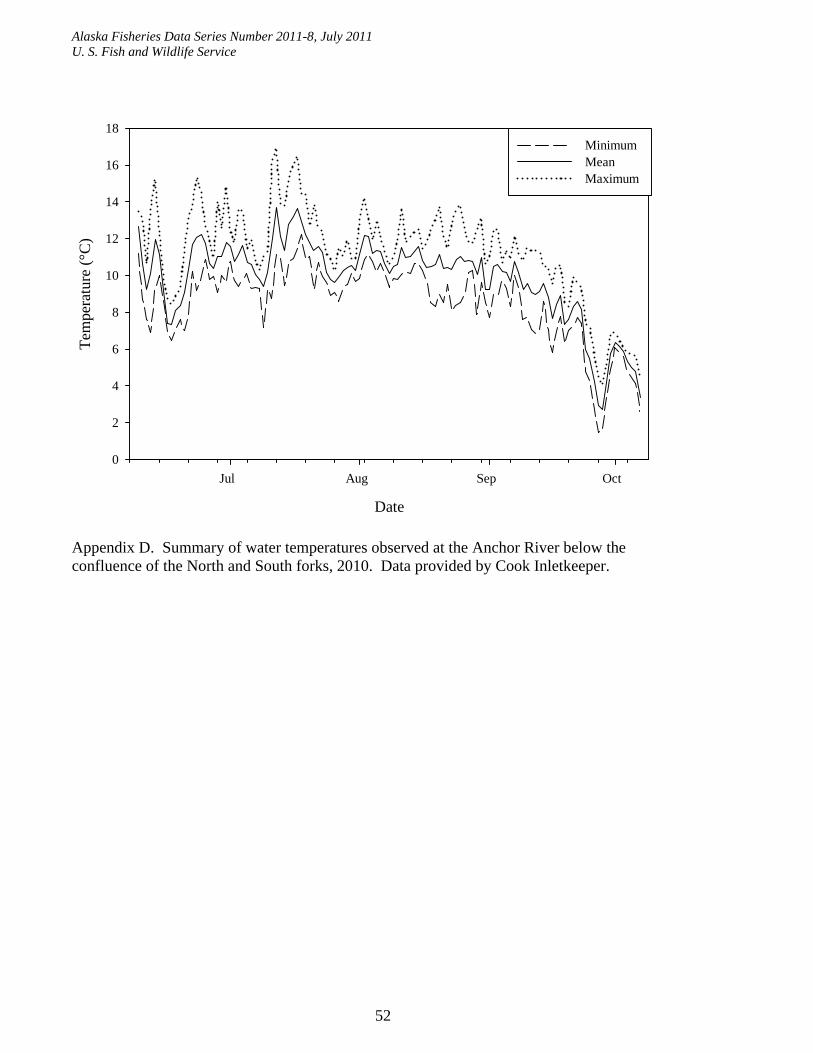
Alaska Fisheries Data Series Number 2011-8, July 2011 U. S. Fish and Wildlife Service
52
Date
Jul Aug Sep Oct
Tem
pera
ture
(°C
)
0
2
4
6
8
10
12
14
16
18MinimumMean Maximum
Appendix D. Summary of water temperatures observed at the Anchor River below the confluence of the North and South forks, 2010. Data provided by Cook Inletkeeper.
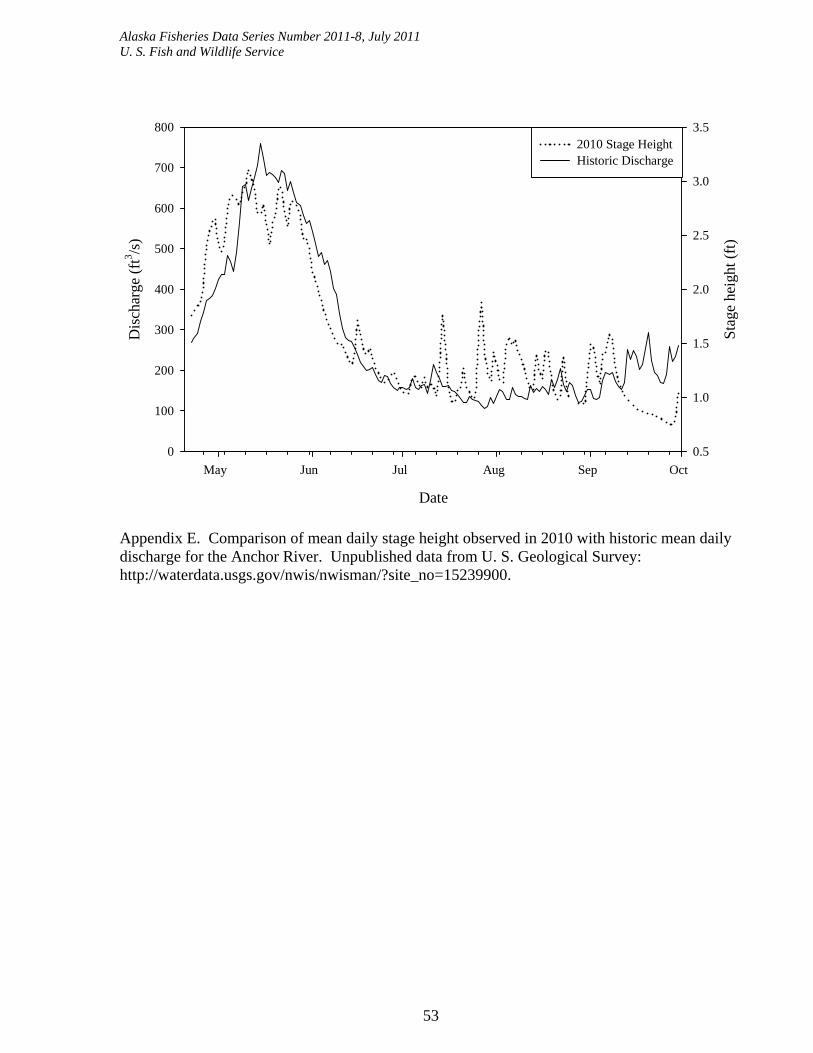
Alaska Fisheries Data Series Number 2011-8, July 2011 U. S. Fish and Wildlife Service
53
Date
May Jun Jul Aug Sep Oct
Sta
ge h
eigh
t (ft
)
0.5
1.0
1.5
2.0
2.5
3.0
3.5D
isch
arge
(ft
3 /s)
0
100
200
300
400
500
600
700
8002010 Stage HeightHistoric Discharge
Appendix E. Comparison of mean daily stage height observed in 2010 with historic mean daily discharge for the Anchor River. Unpublished data from U. S. Geological Survey: http://waterdata.usgs.gov/nwis/nwisman/?site_no=15239900.