Embed Size (px)
Citation preview
CISM 2.1 Documentation
William Lipscomb1,2, Stephen Price1, Matthew Hoffman1, Gunter R. Leguy 2,Magnus Hagdorn3, Ian Rutt4, Tony Payne5, Felix Hebeler6, Joseph H. Kennedy 7
June 17, 2018
1Group T-3, Fluid Dynamics and Solid Mechanics, Los Alamos National Laboratory2Climate and Global Dynamics Laboratory, National Center for Atmospheric Research3School of GeoSciences, University of Edinburgh4Department of Geography, Swansea University5School of Geographical Sciences, University of Bristol6Department of Geography, University of Zurich (original affiliation while working on project)7Computational Earth Sciences Group, Oak Ridge National Laboratory

ii
CISM2 Code Developers
Erin Barker (Los Alamos National Laboratory*), Tim Bocek (University of Montana, Mis-soula*), Josh Campbell (University of Montana, Missoula), Katherine J. Evans (Oak RidgeNational Laboratory), Jeremy Fyke (Los Alamos National Laboratory*), Glen Granzow (Uni-versity of Montana, Missoula), Magnus Hagdorn (School of GeoSciences, University of Edin-burgh), Brian Hand (University of Montana, Missoula*), Felix Hebeler (University of Zurich*),Matthew Hoffman (Los Alamos National Laboratory), Jesse Johnson (University of Montana,Missoula), Irina Kalashnikova (Sandia National Laboratories), Joseph H. Kennedy (Oak RidgeNational Laboratory), Gunter R. Leguy (National Center for Atmospheric Research), Jean-Francois Lemieux (New York University*), William Lipscomb (Los Alamos National Labora-tory), Daniel Martin (Lawrence Berkeley National Laboratory), Jeffrey A. Nichols (Oak RidgeNational Laboratory), Ryan Nong (Sandia National Laboratories*), Matthew R. Norman (OakRidge National Laboratory), Tony Payne (University of Bristol), Stephen Price (Los AlamosNational Laboratory), Doug Ranken (Los Alamos National Laboratory), Ian Rutt (Departmentof Geography, Swansea University), William Sacks (National Center for Atmospheric Research),Andrew Salinger (Sandia National Laboratories), James B. White III (Oak Ridge National Lab-oratory*), Jon Wolfe (National Center for Atmospheric Research*), Patrick Worley (Oak RidgeNational Laboratory), Timothy Wylie (University of Montana, Missoula*),
* author’s original affiliation while working on project
iii

iv
Funding
CISM development was supported primarily by the Earth System Modeling program, Office ofBiological and Envi- 15 ronmental Research (BER) of the U.S. Department of Energys Officeof Science. Additional support was provided by the DOEs Office of Advanced Scientific Com-puting Research (ASCR), by BERs Regional and Global Climate Modeling Program, and bythe National Sci- ence Foundation. The National Center for Atmospheric Research is sponsoredby the National Science Foundation. CISM has evolved from the Glimmer model which wassupported by the U.K. National Environmental Research Council (through the Centre for Polarand Ocean Modelling).
v

vi
Contents
I User Documentation 1
1 Introduction and Overview 31.1 Introduction . . . . . . . . . . . . . . . . . . . . . . . . . . . . . . . . . . . . . . . 31.2 Overview . . . . . . . . . . . . . . . . . . . . . . . . . . . . . . . . . . . . . . . . 3
2 Installing CISM 52.1 Getting and Installing CISM . . . . . . . . . . . . . . . . . . . . . . . . . . . . . 52.2 Installing Supporting Software for Basic (Serial) CISM . . . . . . . . . . . . . . . 6
2.2.1 Install git version control software . . . . . . . . . . . . . . . . . . . . . . 72.2.2 Install the GCC compiler suite . . . . . . . . . . . . . . . . . . . . . . . . 82.2.3 Install build tools . . . . . . . . . . . . . . . . . . . . . . . . . . . . . . . . 92.2.4 Install netCDF . . . . . . . . . . . . . . . . . . . . . . . . . . . . . . . . . 92.2.5 Install Python and related modules . . . . . . . . . . . . . . . . . . . . . . 10
2.3 Building Serial CISM . . . . . . . . . . . . . . . . . . . . . . . . . . . . . . . . . . 112.4 Installing Supporting Software for Parallel CISM . . . . . . . . . . . . . . . . . . 14
2.4.1 Install MPI . . . . . . . . . . . . . . . . . . . . . . . . . . . . . . . . . . . 142.4.2 Install Trilinos solver libraries . . . . . . . . . . . . . . . . . . . . . . . . . 15
2.5 Building Parallel CISM . . . . . . . . . . . . . . . . . . . . . . . . . . . . . . . . 172.6 Next Steps . . . . . . . . . . . . . . . . . . . . . . . . . . . . . . . . . . . . . . . 17
3 Introduction to Ice Sheet Modeling: Derivation of Field Equations 193.1 Conservation Equations . . . . . . . . . . . . . . . . . . . . . . . . . . . . . . . . 19
3.1.1 Integral form . . . . . . . . . . . . . . . . . . . . . . . . . . . . . . . . . . 193.1.2 Derivative form . . . . . . . . . . . . . . . . . . . . . . . . . . . . . . . . . 20
3.2 Applications of the General Conservation Equation . . . . . . . . . . . . . . . . . 213.2.1 Conservation of momentum . . . . . . . . . . . . . . . . . . . . . . . . . . 213.2.2 Conservation of energy . . . . . . . . . . . . . . . . . . . . . . . . . . . . . 233.2.3 Conservation of mass . . . . . . . . . . . . . . . . . . . . . . . . . . . . . . 23
4 Shallow Ice Dynamics: Glide Dynamical Core 274.1 Ice Thickness Evolution . . . . . . . . . . . . . . . . . . . . . . . . . . . . . . . . 27
4.1.1 Numerical grid . . . . . . . . . . . . . . . . . . . . . . . . . . . . . . . . . 284.1.2 Ice sheet equations in σ–coordinates . . . . . . . . . . . . . . . . . . . . . 314.1.3 Calculating the horizontal velocity and diffusivity . . . . . . . . . . . . . . 314.1.4 Solving the ice thickness evolution equation . . . . . . . . . . . . . . . . . 324.1.5 Calculating vertical velocities . . . . . . . . . . . . . . . . . . . . . . . . . 34
4.2 Temperature Solver . . . . . . . . . . . . . . . . . . . . . . . . . . . . . . . . . . . 364.2.1 Vertical diffusion . . . . . . . . . . . . . . . . . . . . . . . . . . . . . . . . 374.2.2 Horizontal advection . . . . . . . . . . . . . . . . . . . . . . . . . . . . . . 384.2.3 Heat generation . . . . . . . . . . . . . . . . . . . . . . . . . . . . . . . . . 384.2.4 Vertical advection . . . . . . . . . . . . . . . . . . . . . . . . . . . . . . . 39
vii
viii CONTENTS
4.2.5 Boundary conditions . . . . . . . . . . . . . . . . . . . . . . . . . . . . . . 394.2.6 Putting it all together . . . . . . . . . . . . . . . . . . . . . . . . . . . . . 40
4.3 Basal Boundary Condition . . . . . . . . . . . . . . . . . . . . . . . . . . . . . . . 414.3.1 Mechanical boundary conditions . . . . . . . . . . . . . . . . . . . . . . . 414.3.2 Thermal boundary conditions . . . . . . . . . . . . . . . . . . . . . . . . . 424.3.3 Numerical solution . . . . . . . . . . . . . . . . . . . . . . . . . . . . . . . 434.3.4 Basal hydrology . . . . . . . . . . . . . . . . . . . . . . . . . . . . . . . . 444.3.5 Putting it all together . . . . . . . . . . . . . . . . . . . . . . . . . . . . . 44
4.4 Isostatic Adjustment . . . . . . . . . . . . . . . . . . . . . . . . . . . . . . . . . . 444.4.1 Calculation of ice-water load . . . . . . . . . . . . . . . . . . . . . . . . . 464.4.2 Elastic lithosphere model . . . . . . . . . . . . . . . . . . . . . . . . . . . 464.4.3 Relaxing asthenosphere model . . . . . . . . . . . . . . . . . . . . . . . . 47
4.5 Time Step Ordering . . . . . . . . . . . . . . . . . . . . . . . . . . . . . . . . . . 47
5 Introduction to Higher-Order Ice Dynamics 495.1 Higher-Order Dynamics in CISM . . . . . . . . . . . . . . . . . . . . . . . . . . . 49
5.1.1 Basics . . . . . . . . . . . . . . . . . . . . . . . . . . . . . . . . . . . . . . 495.1.2 Available schemes . . . . . . . . . . . . . . . . . . . . . . . . . . . . . . . 505.1.3 Shallow-ice vs. higher-order models: practical differences . . . . . . . . . 51
5.2 Higher-Order Momentum Balance . . . . . . . . . . . . . . . . . . . . . . . . . . 535.3 Higher-Order Model Boundary Conditions . . . . . . . . . . . . . . . . . . . . . . 56
5.3.1 Stress-free surface . . . . . . . . . . . . . . . . . . . . . . . . . . . . . . . 565.3.2 Specified basal traction . . . . . . . . . . . . . . . . . . . . . . . . . . . . 575.3.3 Specified basal yield stress . . . . . . . . . . . . . . . . . . . . . . . . . . . 595.3.4 Lateral boundary conditions . . . . . . . . . . . . . . . . . . . . . . . . . . 595.3.5 Summary . . . . . . . . . . . . . . . . . . . . . . . . . . . . . . . . . . . . 62
5.4 Numerical Solution of Higher-Order Equations . . . . . . . . . . . . . . . . . . . 625.4.1 Governing matrix equations . . . . . . . . . . . . . . . . . . . . . . . . . . 625.4.2 Treating nonlinearity through a fixed-point iteration . . . . . . . . . . . . 63
5.5 Thickness Evolution in Higher-Order Models . . . . . . . . . . . . . . . . . . . . 635.5.1 Conservation of mass . . . . . . . . . . . . . . . . . . . . . . . . . . . . . . 635.5.2 A diffusive approach . . . . . . . . . . . . . . . . . . . . . . . . . . . . . . 645.5.3 Advection schemes . . . . . . . . . . . . . . . . . . . . . . . . . . . . . . . 645.5.4 Explicit vs. implicit evolution schemes . . . . . . . . . . . . . . . . . . . . 66
6 Higher-Order Ice Dynamics: Glissade Dynamical Core 676.1 Introduction . . . . . . . . . . . . . . . . . . . . . . . . . . . . . . . . . . . . . . . 676.2 Velocity Solver . . . . . . . . . . . . . . . . . . . . . . . . . . . . . . . . . . . . . 68
6.2.1 Blatter-Pattyn approximation . . . . . . . . . . . . . . . . . . . . . . . . . 686.2.2 Shallow-ice approximation . . . . . . . . . . . . . . . . . . . . . . . . . . . 806.2.3 Shallow-shelf approximation . . . . . . . . . . . . . . . . . . . . . . . . . . 826.2.4 Depth-integrated-viscosity approximation . . . . . . . . . . . . . . . . . . 836.2.5 L1L2 approximation . . . . . . . . . . . . . . . . . . . . . . . . . . . . . . 85
6.3 Temperature Solver . . . . . . . . . . . . . . . . . . . . . . . . . . . . . . . . . . . 886.3.1 Vertical diffusion . . . . . . . . . . . . . . . . . . . . . . . . . . . . . . . . 886.3.2 Heat dissipation . . . . . . . . . . . . . . . . . . . . . . . . . . . . . . . . 896.3.3 Boundary conditions . . . . . . . . . . . . . . . . . . . . . . . . . . . . . . 906.3.4 Vertical temperature solution . . . . . . . . . . . . . . . . . . . . . . . . . 906.3.5 Enthalpy model . . . . . . . . . . . . . . . . . . . . . . . . . . . . . . . . . 91
6.4 Mass and Tracer Transport . . . . . . . . . . . . . . . . . . . . . . . . . . . . . . 916.4.1 Incremental remapping . . . . . . . . . . . . . . . . . . . . . . . . . . . . 926.4.2 CFL checks . . . . . . . . . . . . . . . . . . . . . . . . . . . . . . . . . . . 98
6.5 Basal physics . . . . . . . . . . . . . . . . . . . . . . . . . . . . . . . . . . . . . . 99
CONTENTS ix
6.6 Calving . . . . . . . . . . . . . . . . . . . . . . . . . . . . . . . . . . . . . . . . . 1016.7 Other model physics . . . . . . . . . . . . . . . . . . . . . . . . . . . . . . . . . . 102
7 Running CISM 1037.1 Overview of Running CISM . . . . . . . . . . . . . . . . . . . . . . . . . . . . . . 1037.2 Overview of Configuration Files . . . . . . . . . . . . . . . . . . . . . . . . . . . . 1047.3 Model Configuration . . . . . . . . . . . . . . . . . . . . . . . . . . . . . . . . . . 1057.4 Input/Output Configuration . . . . . . . . . . . . . . . . . . . . . . . . . . . . . . 1137.5 Climate Forcing Configuration . . . . . . . . . . . . . . . . . . . . . . . . . . . . 115
7.5.1 EISMINT climate forcing . . . . . . . . . . . . . . . . . . . . . . . . . . . 1157.5.2 Glint driver . . . . . . . . . . . . . . . . . . . . . . . . . . . . . . . . . . . 117
7.6 Glint: Using glint-example . . . . . . . . . . . . . . . . . . . . . . . . . . . . . . . 1227.7 Supplied mass-balance schemes . . . . . . . . . . . . . . . . . . . . . . . . . . . . 123
7.7.1 Annual PDD scheme . . . . . . . . . . . . . . . . . . . . . . . . . . . . . . 1237.7.2 Daily PDD scheme . . . . . . . . . . . . . . . . . . . . . . . . . . . . . . . 125
8 Test Cases 1278.1 Shallow-Ice Test Cases . . . . . . . . . . . . . . . . . . . . . . . . . . . . . . . . . 127
8.1.1 Halfar dome . . . . . . . . . . . . . . . . . . . . . . . . . . . . . . . . . . . 1288.1.2 EISMINT-1 . . . . . . . . . . . . . . . . . . . . . . . . . . . . . . . . . . . 1298.1.3 EISMINT-2 . . . . . . . . . . . . . . . . . . . . . . . . . . . . . . . . . . . 1308.1.4 Glint example . . . . . . . . . . . . . . . . . . . . . . . . . . . . . . . . . . 130
8.2 Higher-Order Test Cases . . . . . . . . . . . . . . . . . . . . . . . . . . . . . . . . 1318.2.1 Dome . . . . . . . . . . . . . . . . . . . . . . . . . . . . . . . . . . . . . . 1318.2.2 ISMIP-HOM . . . . . . . . . . . . . . . . . . . . . . . . . . . . . . . . . . 1338.2.3 Stream . . . . . . . . . . . . . . . . . . . . . . . . . . . . . . . . . . . . . 1348.2.4 Confined shelf . . . . . . . . . . . . . . . . . . . . . . . . . . . . . . . . . . 1368.2.5 Circular shelf . . . . . . . . . . . . . . . . . . . . . . . . . . . . . . . . . . 1388.2.6 Ross Ice Shelf . . . . . . . . . . . . . . . . . . . . . . . . . . . . . . . . . . 1398.2.7 MISMIP . . . . . . . . . . . . . . . . . . . . . . . . . . . . . . . . . . . . . 1418.2.8 MISMIP3d . . . . . . . . . . . . . . . . . . . . . . . . . . . . . . . . . . . 1448.2.9 MISMIP+ . . . . . . . . . . . . . . . . . . . . . . . . . . . . . . . . . . . . 1468.2.10 Other tests . . . . . . . . . . . . . . . . . . . . . . . . . . . . . . . . . . . 148
8.3 The build and test structure (BATS) . . . . . . . . . . . . . . . . . . . . . . . . . 148
II Appendix 151
A NetCDF Variables 153A.1 Glide/Glissade Variables . . . . . . . . . . . . . . . . . . . . . . . . . . . . . . . . 153A.2 Glint Variables . . . . . . . . . . . . . . . . . . . . . . . . . . . . . . . . . . . . . 159
B Input and Output (I/O) 161B.1 NetCDF I/O . . . . . . . . . . . . . . . . . . . . . . . . . . . . . . . . . . . . . . 161
B.1.1 Data structures . . . . . . . . . . . . . . . . . . . . . . . . . . . . . . . . . 161B.1.2 Code generator . . . . . . . . . . . . . . . . . . . . . . . . . . . . . . . . . 161B.1.3 Variable definition file . . . . . . . . . . . . . . . . . . . . . . . . . . . . . 161
C Commonly Used Notation 163
III Bibliography 165

x CONTENTS
Part I
User Documentation
1

Chapter 1
Introduction and Overview
1.1 Introduction
CISM, the Community Ice Sheet Model, originates from the Glimmer and Glimmer–CISMprojects (Rutt et al., 2009)1. The current name reflects the project’s evolution from a stand-alone ice sheet model to a fully supported, coupled component of the Community Earth SystemModel, or CESM. CISM is a numerical model—a collection of software libraries, utilities anddrivers— used to simulate ice sheet evolution. CISM is modular in design and coded almostentirely in standards-compliant Fortran 95. It currently supports two different dynamical cores(“dycores”), which solve the equations for conservation of mass, energy, and momentum. Aswith previous versions of Glimmer and Glimmer-CISM, the current version of CISM supportsa serial, shallow-ice representation of ice dynamics. New with CISM2 are support for “higher-order” ice dynamics, scalable parallelism, and software links for coupling to modern, robust,C++ based, third-party solver libraries.
1.2 Overview
CISM consists of several components:
• cism driver: the high-level driver (i.e., the executable) that is used to run the ice sheetmodel. Unlike the drivers in previous versions of Glimmer and Glimmer-CISM, cism driveris used to run the code in all model configurations (e.g., for idealized test cases withsimplified climate forcing and for model runs based on realistic geometries and climateforcing data).
• Glide: the dynamical core based on shallow-ice dynamics. This component is responsiblefor solving the governing conservation equations and determining ice velocities, internalice temperature, and ice geometry evolution (see Chapter 4). Apart from minor changes,this is the same shallow-ice dynamical core used by Glimmer and Glimmer-CISM.
• Glissade: the dynamical core based on a first-order-accurate approximation of the Stokesequations for ice flow. This dycore, like Glide, solves the governing conservation equa-tions. Unlike Glide, Glissade is fully parallel in order to take advantage of modern, multi-processor, high-performance architectures (see Chapter 6).
• Glint: the climate model interface. Glint allows the core ice sheet model to be coupledto a variety of global climate models, or indeed any source of time-varying climate dataon a lat-lon grid.
1 Glimmer was originally an acronym for GENIE Land Ice Model with Multiply Enabled Regions, reflectingthe project’s origin within the GENIE (Grid ENabled Integrated Earth-system) model.
3
4 CHAPTER 1. INTRODUCTION AND OVERVIEW
• Test cases: idealized test cases for the Glide and Glissade dynamical cores and for theGlint climate interface. These are used to (1) confirm that the model is working asexpected and (2) provide a range of simple model configurations from which new userscan learn about model options and create their own configurations (see Chapter 8).
• Shared code: a number of modules shared by different parts of the code. Examplesinclude modules for defining derived types, physical constants, and model parameters,and modules that handle parsing of the configuration file and data input/output (I/O),as discussed below.
Each component is configured using a configuration file (*.config) similar to Windows .inifiles. At run-time, the model configuration is written to a log file.
1D, 2D, and 3D data are written and read to and from netCDF files using the CF (Climate-Forecast) metadata convention2. NetCDF is a scientific data format for storing multidimensionaldata in a platform- and language-independent binary format. The CF conventions specify themetadata used to describe the file contents. Many programs (e.g., Python, Matlab, OpenDX,Ferret, and IDL) can process and visualize netCDF data.
2http://cfconventions.org/
Chapter 2
Installing CISM
2.1 Getting and Installing CISM
CISM1 is a relatively complex system of libraries and programs which build on other libraries.This section documents how to download and install CISM and its prerequisites. Many commonproblems and questions can be addressed using the user discussion boards2 . A CISM users mail-ing list is also available and can be subscribed to by sending an email to [email protected] report unresolved problems using the bug reporting facility at the CISM Github website4.
CISM is distributed as source code, and a reasonably complete build environment is there-fore required to compile the model. For UNIX and LINUX based systems (including Mac),the CMake build system is used to build the model. Sample build scripts for a number ofstandard architectures are included, as are working build scripts for a number of large-scale,high-performance-computing architectures (e.g., Cheyenne (CISL), Titan (OLCF), and Edison(NERSC) ).
There are two ways to get the source code:
1. Download5 a released version of the code as an archive (.zip or .tar.gz file).
2. Clone the code from the CISM Github repository6 using the following command: git
clone https://github.com/CISM/cism.git (It is also possible to clone the repositoryusing the SSH protocol if you have an SSH keypair generated on your computer andattached to your GitHub account. See the CISM Github repository webpage and Github’shelp pages for more information.)
For beginners, downloading a zip archive of the latest release tag is recommended. Moreexperienced users may want to download directly from the repository, as it will make updatingthe code easier in the future.
In either case, a Fortran90 compiler is required. Other software dependencies include thenetCDF library (used for data I/O) and a Python distribution (used to analyze dependenciesand to automatically generate parts of the code) with a number of specific Python modules.Users who want to run the code in parallel will need to install MPI, and users who want accessto the Trilinos solver library will need to download and build Trilinos, and link to it when
1https://cism.github.io/2http://forum.cgd.ucar.edu/forums/ice-sheet-modeling-cism3In order to subscribe from a non-Google email address, you should first make sure to completely log out from
any Google sites (e.g., Gmail) before sending your request. If you do not, it will automatically try to associateyour request with your Gmail account instead.
4https://github.com/CISM/cism/issues5https://github.com/CISM/cism/releases6https://github.com/CISM/cism
5
6 CHAPTER 2. INSTALLING CISM
building CISM. Finally, you will need CMake and Gnu Make to compile the code and link tothe various third-party libraries.
If you have not done so already, clone a tagged version of CISM or download an archiveof the code, as noted above. Store the code or the unzipped/untarred archive in a locationof your choice. More detailed build instructions, including instructions for the installation ofsupporting software, are given below.
2.2 Installing Supporting Software for Basic (Serial) CISM
Because the build process can be fairly complicated, we describe it in detail below, relying onthe use of a package manager to handle many of the standard software dependencies. For eachstep we give specific instructions for both Mac OS X using MacPorts (in red boxes) and Linux(in blue boxes). For the former the instructions work for Mac OS High Sierra. For the latter,we have verified that the instructions work for Ubuntu 12.10 and 14.04 LTS. For different butrelated systems, hopefully these instructions can be used as a guide.
CISM can be installed in either a serial or parallel configuration. The parallel mode allowsthe model to be run on multiple processors which can greatly speed up execution. This is acommon configuration to use on supercomputing clusters, but can also be convenient on moderndesktops and laptops which often have four or more cores available. However, the parallel buildrequires additional supporting software, so we first detail how to build serial CISM. For newusers, it is recommended to first build and successfully run serial CISM before moving on tothe parallel build.
Note: Glide, the shallow-ice dycore, can only run on a single processor, even when the codeis built with full parallel support. This is also true of the SLAP solver routines.
The instructions below assume the user has administrative privileges for installing newsoftware (note the extensive use of sudo). If you are working on a shared machine withoutadministrative privileges, you might proceed by assuming all needed packages are present andcontinue to the CISM installation section. If you encounter problems, you can refer back to thissection to determine which packages might be missing or problematic before contacting yoursystem administrator.
Mac OS X
As mentioned above, we will take advantage of MacPorts, a software package managerfor Macs. This will allow us to install most of the base level software libraries needed byCISM with few complications.
Go to http://www.macports.org/install.php, where you will find a range of ”.pkg”installs available, including those for Mountain Lion, Lion, and Mavericks versions of MacOS X.
Installing MacPorts requires installing the Xcode developer toolset provided by Apple.Details of how to obtain Xcode vary by version of OS X. See MacPorts installation in-structions and this link for details. Once Xcode is installed, you may need to additionallydownload the “command line tool” from the Preferences / Downloads menu of Xcode.
Depending on computer security settings at your institution (firewalls, etc.), you mayneed to add proxy information so that Macports can communicate and download soft-ware from the outside world. All Macports software will be installed under /opt/local/by default. To add proxy information, after installing Macports, edit the configurationfile at /opt/local/etc/macports/macports.conf. (Note this is probably a read-onlyfile that requires superuser permission to edit, so you will need to edit the file withsomething like: sudo vim /opt/local/etc/macports/macports.conf). By searchingfor the text string “proxy”, you will find the lines like proxy http hostname:12345
2.2. INSTALLING SUPPORTING SOFTWARE FOR BASIC (SERIAL) CISM 7
near the bottom of the file. Enter your proxy information here as appropriate (e.g.,hostname:your host info here).
If you have previously installed Macports but not updated it recently, it’s generally agood idea to do so. Ideally, this should be done with admin or root privileges (you willbe prompted to enter your password) using:
sudo port selfupdate
You will then be prompted to update any installed ports that are outdated, which youcan do using:
sudo port upgrade outdated
To search for available software in Macports, type:port search software-name
Software is installed through Macports using the command:sudo port install software-name
Additional Macports tips will follow inline below. Extensive documentation for Macportscan be found at the Macports website.
Ubuntu 12.10
This Ubuntu instructions describe setting up supporting software and CISM in a Linuxenvironment. These instructions were written using a fresh installation of Ubuntu 12.10but steps should be very similar in other versions of Ubuntu or other distributions ofLinux. Instructions make use of the command line tool for installing packages that comeswith Ubuntu, apt-get. Other package management tools (e.g., Software Center) couldalso be used.
It’s generally a good idea to synchronize your local package index files before installingnew software using apt-get:
sudo apt-get update
To search for available packages, type:apt-cache search software-name
And to see detailed information about a package, type:apt-cache show software-name
Packages are installed through apt-get using the command:sudo apt-get install software-name
Some users have reported that BLAS and LAPACK libraries need to installed explicitly,for example when starting from a “clean” machine. To do this, use the following twocommands:
sudo apt-get install libblas-dev
andsudo apt-get install liblapack-dev
Additional apt-get tips will follow inline below. Extensive documentation for apt-get canbe found at the Ubuntu website and through man pages (man apt-get).
2.2.1 Install git version control software
If you intend to download the CISM code as a git repository, you will need the git packageinstalled. If you prefer to download a zipped archive of the code, this step can be skipped.
Mac OS X
Install git with:
8 CHAPTER 2. INSTALLING CISM
sudo port install git
Ubuntu 12.10
Install git with:sudo apt-get install git
2.2.2 Install the GCC compiler suite
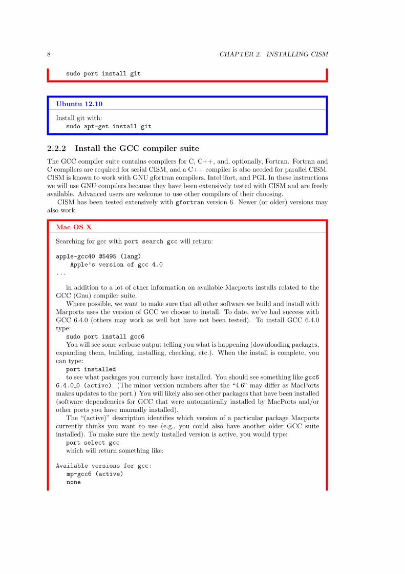
The GCC compiler suite contains compilers for C, C++, and, optionally, Fortran. Fortran andC compilers are required for serial CISM, and a C++ compiler is also needed for parallel CISM.CISM is known to work with GNU gfortran compilers, Intel ifort, and PGI. In these instructionswe will use GNU compilers because they have been extensively tested with CISM and are freelyavailable. Advanced users are welcome to use other compilers of their choosing.
CISM has been tested extensively with gfortran version 6. Newer (or older) versions mayalso work.
Mac OS X
Searching for gcc with port search gcc will return:
apple-gcc40 @5495 (lang)
Apple’s version of gcc 4.0
...
in addition to a lot of other information on available Macports installs related to theGCC (Gnu) compiler suite.
Where possible, we want to make sure that all other software we build and install withMacports uses the version of GCC we choose to install. To date, we’ve had success withGCC 6.4.0 (others may work as well but have not been tested). To install GCC 6.4.0type:
sudo port install gcc6
You will see some verbose output telling you what is happening (downloading packages,expanding them, building, installing, checking, etc.). When the install is complete, youcan type:
port installed
to see what packages you currently have installed. You should see something like gcc66.4.0 0 (active). (The minor version numbers after the “4.6” may differ as MacPortsmakes updates to the port.) You will likely also see other packages that have been installed(software dependencies for GCC that were automatically installed by MacPorts and/orother ports you have manually installed).
The “(active)” description identifies which version of a particular package Macportscurrently thinks you want to use (e.g., you could also have another older GCC suiteinstalled). To make sure the newly installed version is active, you would type:
port select gcc
which will return something like:
Available versions for gcc:
mp-gcc6 (active)
none
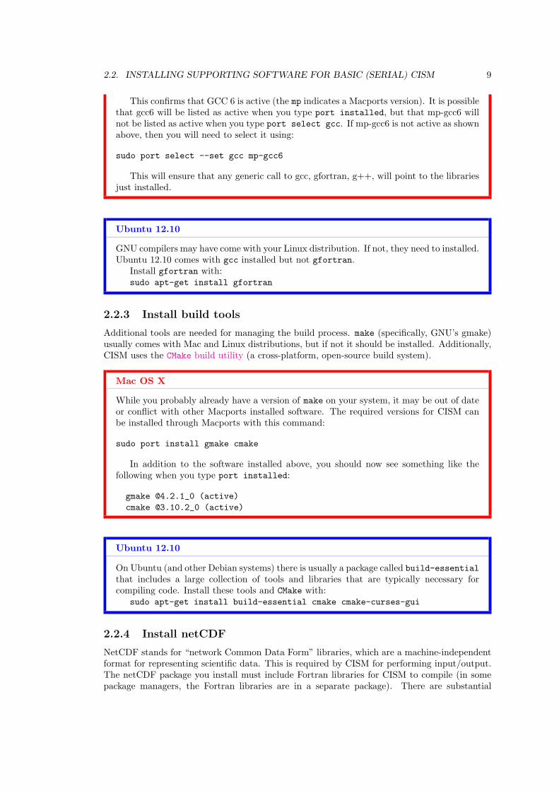
2.2. INSTALLING SUPPORTING SOFTWARE FOR BASIC (SERIAL) CISM 9
This confirms that GCC 6 is active (the mp indicates a Macports version). It is possiblethat gcc6 will be listed as active when you type port installed, but that mp-gcc6 willnot be listed as active when you type port select gcc. If mp-gcc6 is not active as shownabove, then you will need to select it using:
sudo port select --set gcc mp-gcc6
This will ensure that any generic call to gcc, gfortran, g++, will point to the librariesjust installed.
Ubuntu 12.10
GNU compilers may have come with your Linux distribution. If not, they need to installed.Ubuntu 12.10 comes with gcc installed but not gfortran.
Install gfortran with:sudo apt-get install gfortran
2.2.3 Install build tools
Additional tools are needed for managing the build process. make (specifically, GNU’s gmake)usually comes with Mac and Linux distributions, but if not it should be installed. Additionally,CISM uses the CMake build utility (a cross-platform, open-source build system).
Mac OS X
While you probably already have a version of make on your system, it may be out of dateor conflict with other Macports installed software. The required versions for CISM canbe installed through Macports with this command:
sudo port install gmake cmake
In addition to the software installed above, you should now see something like thefollowing when you type port installed:
gmake @4.2.1_0 (active)
cmake @3.10.2_0 (active)
Ubuntu 12.10
On Ubuntu (and other Debian systems) there is usually a package called build-essential
that includes a large collection of tools and libraries that are typically necessary forcompiling code. Install these tools and CMake with:
sudo apt-get install build-essential cmake cmake-curses-gui
2.2.4 Install netCDF
NetCDF stands for “network Common Data Form” libraries, which are a machine-independentformat for representing scientific data. This is required by CISM for performing input/output.The netCDF package you install must include Fortran libraries for CISM to compile (in somepackage managers, the Fortran libraries are in a separate package). There are substantial
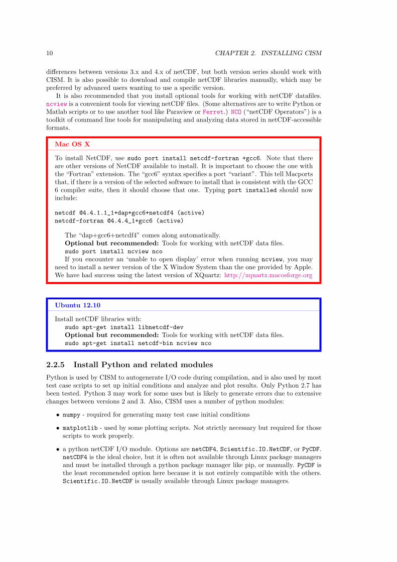
10 CHAPTER 2. INSTALLING CISM
differences between versions 3.x and 4.x of netCDF, but both version series should work withCISM. It is also possible to download and compile netCDF libraries manually, which may bepreferred by advanced users wanting to use a specific version.
It is also recommended that you install optional tools for working with netCDF datafiles.ncview is a convenient tools for viewing netCDF files. (Some alternatives are to write Python orMatlab scripts or to use another tool like Paraview or Ferret.) NCO (“netCDF Operators”) is atoolkit of command line tools for manipulating and analyzing data stored in netCDF-accessibleformats.
Mac OS X
To install NetCDF, use sudo port install netcdf-fortran +gcc6. Note that thereare other versions of NetCDF available to install. It is important to choose the one withthe “Fortran” extension. The “gcc6” syntax specifies a port “variant”. This tell Macportsthat, if there is a version of the selected software to install that is consistent with the GCC6 compiler suite, then it should choose that one. Typing port installed should nowinclude:
netcdf @4.4.1.1_1+dap+gcc6+netcdf4 (active)
netcdf-fortran @4.4.4_1+gcc6 (active)
The “dap+gcc6+netcdf4” comes along automatically.Optional but recommended: Tools for working with netCDF data files.sudo port install ncview nco
If you encounter an ‘unable to open display’ error when running ncview, you mayneed to install a newer version of the X Window System than the one provided by Apple.We have had success using the latest version of XQuartz: http://xquartz.macosforge.org
Ubuntu 12.10
Install netCDF libraries with:sudo apt-get install libnetcdf-dev
Optional but recommended: Tools for working with netCDF data files.sudo apt-get install netcdf-bin ncview nco
2.2.5 Install Python and related modules
Python is used by CISM to autogenerate I/O code during compilation, and is also used by mosttest case scripts to set up initial conditions and analyze and plot results. Only Python 2.7 hasbeen tested. Python 3 may work for some uses but is likely to generate errors due to extensivechanges between versions 2 and 3. Also, CISM uses a number of python modules:
• numpy - required for generating many test case initial conditions
• matplotlib - used by some plotting scripts. Not strictly necessary but required for thosescripts to work properly.
• a python netCDF I/O module. Options are netCDF4, Scientific.IO.NetCDF, or PyCDF.netCDF4 is the ideal choice, but it is often not available through Linux package managersand must be installed through a python package manager like pip, or manually. PyCDF isthe least recommended option here because it is not entirely compatible with the others.Scientific.IO.NetCDF is usually available through Linux package managers.
2.3. BUILDING SERIAL CISM 11
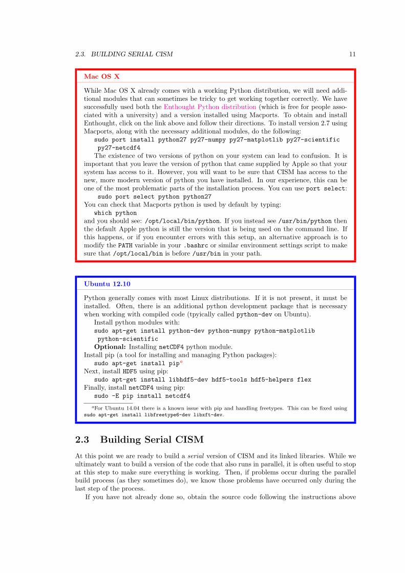
Mac OS X
While Mac OS X already comes with a working Python distribution, we will need addi-tional modules that can sometimes be tricky to get working together correctly. We havesuccessfully used both the Enthought Python distribution (which is free for people asso-ciated with a university) and a version installed using Macports. To obtain and installEnthought, click on the link above and follow their directions. To install version 2.7 usingMacports, along with the necessary additional modules, do the following:
sudo port install python27 py27-numpy py27-matplotlib py27-scientific
py27-netcdf4
The existence of two versions of python on your system can lead to confusion. It isimportant that you leave the version of python that came supplied by Apple so that yoursystem has access to it. However, you will want to be sure that CISM has access to thenew, more modern version of python you have installed. In our experience, this can beone of the most problematic parts of the installation process. You can use port select:
sudo port select python python27
You can check that Macports python is used by default by typing:which python
and you should see: /opt/local/bin/python. If you instead see /usr/bin/python thenthe default Apple python is still the version that is being used on the command line. Ifthis happens, or if you encounter errors with this setup, an alternative approach is tomodify the PATH variable in your .bashrc or similar environment settings script to makesure that /opt/local/bin is before /usr/bin in your path.
Ubuntu 12.10
Python generally comes with most Linux distributions. If it is not present, it must beinstalled. Often, there is an additional python development package that is necessarywhen working with compiled code (tpyically called python-dev on Ubuntu).
Install python modules with:sudo apt-get install python-dev python-numpy python-matplotlib
python-scientific
Optional: Installing netCDF4 python module.Install pip (a tool for installing and managing Python packages):
sudo apt-get install pipa
Next, install HDF5 using pip:sudo apt-get install libhdf5-dev hdf5-tools hdf5-helpers flex
Finally, install netCDF4 using pip:sudo -E pip install netcdf4
aFor Ubuntu 14.04 there is a known issue with pip and handling freetypes. This can be fixed usingsudo apt-get install libfreetype6-dev libxft-dev.
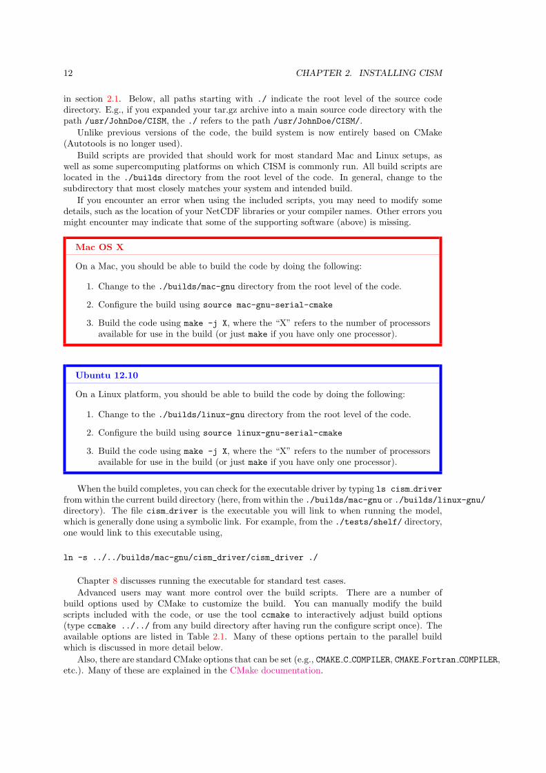
2.3 Building Serial CISM
At this point we are ready to build a serial version of CISM and its linked libraries. While weultimately want to build a version of the code that also runs in parallel, it is often useful to stopat this step to make sure everything is working. Then, if problems occur during the parallelbuild process (as they sometimes do), we know those problems have occurred only during thelast step of the process.
If you have not already done so, obtain the source code following the instructions above
12 CHAPTER 2. INSTALLING CISM
in section 2.1. Below, all paths starting with ./ indicate the root level of the source codedirectory. E.g., if you expanded your tar.gz archive into a main source code directory with thepath /usr/JohnDoe/CISM, the ./ refers to the path /usr/JohnDoe/CISM/.
Unlike previous versions of the code, the build system is now entirely based on CMake(Autotools is no longer used).
Build scripts are provided that should work for most standard Mac and Linux setups, aswell as some supercomputing platforms on which CISM is commonly run. All build scripts arelocated in the ./builds directory from the root level of the code. In general, change to thesubdirectory that most closely matches your system and intended build.
If you encounter an error when using the included scripts, you may need to modify somedetails, such as the location of your NetCDF libraries or your compiler names. Other errors youmight encounter may indicate that some of the supporting software (above) is missing.
Mac OS X
On a Mac, you should be able to build the code by doing the following:
1. Change to the ./builds/mac-gnu directory from the root level of the code.
2. Configure the build using source mac-gnu-serial-cmake
3. Build the code using make -j X, where the “X” refers to the number of processorsavailable for use in the build (or just make if you have only one processor).
Ubuntu 12.10
On a Linux platform, you should be able to build the code by doing the following:
1. Change to the ./builds/linux-gnu directory from the root level of the code.
2. Configure the build using source linux-gnu-serial-cmake
3. Build the code using make -j X, where the “X” refers to the number of processorsavailable for use in the build (or just make if you have only one processor).
When the build completes, you can check for the executable driver by typing ls cism driver
from within the current build directory (here, from within the ./builds/mac-gnu or ./builds/linux-gnu/directory). The file cism driver is the executable you will link to when running the model,which is generally done using a symbolic link. For example, from the ./tests/shelf/ directory,one would link to this executable using,
ln -s ../../builds/mac-gnu/cism_driver/cism_driver ./
Chapter 8 discusses running the executable for standard test cases.
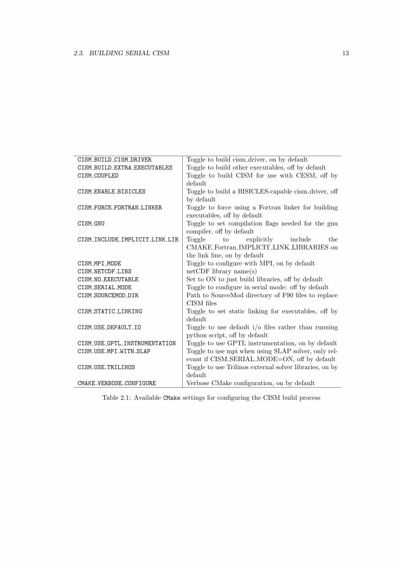
Advanced users may want more control over the build scripts. There are a number ofbuild options used by CMake to customize the build. You can manually modify the buildscripts included with the code, or use the tool ccmake to interactively adjust build options(type ccmake ../../ from any build directory after having run the configure script once). Theavailable options are listed in Table 2.1. Many of these options pertain to the parallel buildwhich is discussed in more detail below.
Also, there are standard CMake options that can be set (e.g., CMAKE C COMPILER, CMAKE Fortran COMPILER,etc.). Many of these are explained in the CMake documentation.
2.3. BUILDING SERIAL CISM 13
CISM BUILD CISM DRIVER Toggle to build cism driver, on by defaultCISM BUILD EXTRA EXECUTABLES Toggle to build other executables, off by defaultCISM COUPLED Toggle to build CISM for use with CESM, off by
defaultCISM ENABLE BISICLES Toggle to build a BISICLES-capable cism driver, off
by defaultCISM FORCE FORTRAN LINKER Toggle to force using a Fortran linker for building
executables, off by defaultCISM GNU Toggle to set compilation flags needed for the gnu
compiler, off by defaultCISM INCLUDE IMPLICIT LINK LIB Toggle to explicitly include the
CMAKE Fortran IMPLICIT LINK LIBRARIES onthe link line, on by default
CISM MPI MODE Toggle to configure with MPI, on by defaultCISM NETCDF LIBS netCDF library name(s)CISM NO EXECUTABLE Set to ON to just build libraries, off by defaultCISM SERIAL MODE Toggle to configure in serial mode: off by defaultCISM SOURCEMOD DIR Path to SourceMod directory of F90 files to replace
CISM filesCISM STATIC LINKING Toggle to set static linking for executables, off by
defaultCISM USE DEFAULT IO Toggle to use default i/o files rather than running
python script, off by defaultCISM USE GPTL INSTRUMENTATION Toggle to use GPTL instrumentation, on by defaultCISM USE MPI WITH SLAP Toggle to use mpi when using SLAP solver, only rel-
evant if CISM SERIAL MODE=ON, off by defaultCISM USE TRILINOS Toggle to use Trilinos external solver libraries, on by
defaultCMAKE VERBOSE CONFIGURE Verbose CMake configuration, on by default
Table 2.1: Available CMake settings for configuring the CISM build process
14 CHAPTER 2. INSTALLING CISM
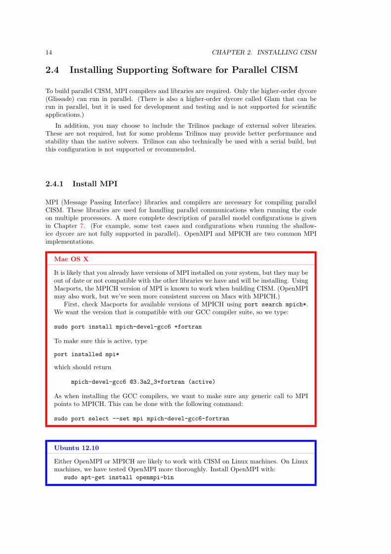
2.4 Installing Supporting Software for Parallel CISM
To build parallel CISM, MPI compilers and libraries are required. Only the higher-order dycore(Glissade) can run in parallel. (There is also a higher-order dycore called Glam that can berun in parallel, but it is used for development and testing and is not supported for scientificapplications.)
In addition, you may choose to include the Trilinos package of external solver libraries.These are not required, but for some problems Trilinos may provide better performance andstability than the native solvers. Trilinos can also technically be used with a serial build, butthis configuration is not supported or recommended.
2.4.1 Install MPI
MPI (Message Passing Interface) libraries and compilers are necessary for compiling parallelCISM. These libraries are used for handling parallel communications when running the codeon multiple processors. A more complete description of parallel model configurations is givenin Chapter 7. (For example, some test cases and configurations when running the shallow-ice dycore are not fully supported in parallel). OpenMPI and MPICH are two common MPIimplementations.
Mac OS X
It is likely that you already have versions of MPI installed on your system, but they may beout of date or not compatible with the other libraries we have and will be installing. UsingMacports, the MPICH version of MPI is known to work when building CISM. (OpenMPImay also work, but we’ve seen more consistent success on Macs with MPICH.)
First, check Macports for available versions of MPICH using port search mpich*.We want the version that is compatible with our GCC compiler suite, so we type:
sudo port install mpich-devel-gcc6 +fortran
To make sure this is active, type
port installed mpi*
which should return
mpich-devel-gcc6 @3.3a2_3+fortran (active)
As when installing the GCC compilers, we want to make sure any generic call to MPIpoints to MPICH. This can be done with the following command:
sudo port select --set mpi mpich-devel-gcc6-fortran
Ubuntu 12.10
Either OpenMPI or MPICH are likely to work with CISM on Linux machines. On Linuxmachines, we have tested OpenMPI more thoroughly. Install OpenMPI with:
sudo apt-get install openmpi-bin
2.4. INSTALLING SUPPORTING SOFTWARE FOR PARALLEL CISM 15
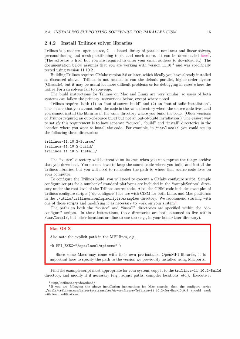
2.4.2 Install Trilinos solver libraries
Trilinos is a modern, open source, C++ based library of parallel nonlinear and linear solvers,preconditioning and mesh-partitioning tools, and much more. It can be downloaded here7.(The software is free, but you are required to enter your email address to download it.) Thedocumentation below assumes that you are working with version 11.10.* and was specificallytested using version 11.10.2.
Building Trilinos requires CMake version 2.8 or later, which ideally you have already installedas discussed above. Trilinos is not needed to run the default parallel, higher-order dycore(Glissade), but it may be useful for more difficult problems or for debugging in cases where thenative Fortran solvers fail to converge.
The build instructions for Trilinos on Mac and Linux are very similar, so users of bothsystems can follow the primary instructions below, except where noted.
Trilinos requires both (1) an “out-of-source build” and (2) an “out-of-build installation”.This means that you cannot build the code in the same directory where the source code lives, andyou cannot install the libraries in the same directory where you build the code. (Older versionsof Trilinos required an out-of-source build but not an out-of-build installation.) The easiest wayto satisfy this requirement is to have separate “source”, “build” and “install” directories in thelocation where you want to install the code. For example, in /usr/local/, you could set upthe following three directories:
trilinos-11.10.2-Source/
trilinos-11.10.2-Build/
trilinos-11.10.2-Install/
The “source” directory will be created on its own when you uncompress the tar.gz archivethat you download. You do not have to keep the source code where you build and install theTrilinos libraries, but you will need to remember the path to where that source code lives onyour computer.
To configure the Trilinos build, you will need to execute a CMake configure script. Sampleconfigure scripts for a number of standard platforms are included in the “sampleScripts” direc-tory under the root level of the Trilinos source code. Also, the CISM code includes examples ofTrilinos configure scripts (“do-configure”) for use with CISM for both Linux and Mac platformsin the ./utils/trilinos config scripts examples directory. We recommend starting withone of those scripts and modifying it as necessary to work on your system8.
The paths to both the “source” and “install” directories are specified within the “do-configure” scripts. In these instructions, those directories are both assumed to live within/usr/local/, but other locations are fine to use too (e.g., in your home/User directory).
Mac OS X
Also note the explicit path in the MPI lines, e.g.,
-D MPI_EXEC="/opt/local/mpiexec" \
Since some Macs may come with their own pre-installed OpenMPI libraries, it isimportant here to specify the path to the version we previously installed using Macports.
Find the example script most appropriate for your system, copy it to the trilinos-11.10.2-Builddirectory, and modify it if necessary (e.g., adjust paths, compiler locations, etc.). Execute it
7http://trilinos.org/download/8If you are following the above installation instructions for Mac exactly, then the configure script
./utils/trilinos config scripts examples/do-configure-Trilinos-11.10.2-for-Mac-10.9.4 should workwith few modifications.
16 CHAPTER 2. INSTALLING CISM
with:source ./do-cmake9
from within your trilinos-11.10.2-Build directory. Depending on where you are buildingand installing the code, you may need to have administrative privileges (in which case youwould type sudo source ./do-cmake). If the configure step was successful, you should see thefollowing displayed on your screen:
...
Processing enabled package: [PACKAGE NAME]
...
Exporting library dependencies ...
Finished configuring Trilinos!
-- Configuring done
-- Generating done
-- Build files have been written to: /usr/local/trilinos-11.10.2-Build
It is a good idea to scan the output while the “do-cmake” script is executing, for example toensure the configure process is picking up the compilers you specified (e.g., it is using the Mac-ports versions as opposed to some Mac default versions that might also be on your system). Oncethe code is configured successfully, build the libraries from within the trilinos-11.10.2-Builddirectory by typing:
make (or sudo make if necessary)For multiprocessor machines, the build process can be sped up significantly using the “-j”commandas described above for building serial CISM:
make -j X
where “X” is the number of cores available on your machine (e.g., make -j 4 for a 2-processor,dual-core machine).
Building Trilinos can take a long time (e.g., an hour or more), depending on your machine,the number of processors used for the build, and the number and type of libraries you areinstalling. Once you have built the code, we highly recommend testing it using:
make test
(The Trilinos ENABLE TESTS:BOOL variable in the do-cmake script can be set to “OFF”todisable building of the tests.) Screen output will tell you if and how many tests failed. We haveseen a few tests fail while still having a perfectly good and working Trilinos library. In general,if the number of tests passed is above 90%, the library will likely work fine with CISM. Querythe CISM users or developers lists10 if you have questions about specific Trilinos tests failing.
Mac OS X
On a Mac, MPI tests have been known to trigger a dialog box from the firewall. With morethan 300 tests, these messages popping up continually can make it impossible to use yourcomputer until the tests complete. To keep them from appearing, you can temporarilyturn off your firewall under “System Preferences” (Security > Firewall > Stop). Be sureto turn the firewall back on when the tests are complete!
After running the tests, you will need to install Trilinos using:
9Here we have assumed that the name of the configure script is “do-cmake”. The script name maydiffer depending on what you have called it or if you copied and modified one of the scripts from./utils/trilinos config scripts examples.
2.5. BUILDING PARALLEL CISM 17
make install
This will build the actual Trilinos libraries in the path specified in the
-D CMAKE_INSTALL_PREFIX:PATH=/path
line of your “do-cmake” script (above). For this example, those libraries will be installed in:/usr/local/trilinos-11.10.2-Install
After successfully building Trilinos, create an environment variable called CISM TRILINOS DIR
so the CISM build process can find the Trilinos installation. For example, if you are using thebash shell and your current directory is the Trilinos install directory, you can do:
export CISM_TRILINOS_DIR=$PWD
You may prefer to modify your .bashrc or .bash profile (or similar) to set this environmentvariable on every login.
Alternatively, you can modify the CISM parallel build script (below) so that the line:
-D CISM_TRILINOS_DIR=$CISM_TRILINOS_DIR \
is set to the Trilinos installation directory.
2.5 Building Parallel CISM
The procedure for building parallel CISM is nearly identical to the serial build (above). Thebuild script for parallel CISM for a Mac is located at builds/mac-gnu/mac-gnu-cmake, whilethe build script for Linux is located at builds/linux-gnu/linux-gnu-cmake. From the appro-priate directory, run:
source mac-gnu-cmake or source linux-gnu-cmake
Once the configuration step completes successfully, you can compile the code as before with:make
ormake -j 4
if you have 4 processors available (or as many processors as you would like to use). See Section2.3 for details about customizing the build process.
Building a parallel version of CISM that includes Trilinos requires setting the
-D CISM_USE_TRILINOS
flag to ON in the builds/mac-gnu/mac-gnu-cmake script.
2.6 Next Steps
If you make any changes to the source code, you only need to re-run make from your builddirectory to generate an updated executable. One exception is that if you edit the lists ofinput/output netCDF variables in * vars.def files (see Appendices A and B), you need to firstre-source the configuration script (e.g., source mac-gnu-cmake) before re-running make.
Now that you have successfully built the code, you can proceed to Chapters 3 and 5 to learnmore detailed information about ice sheet modeling, to Chapters 4 and 6 to learn more aboutthe various model approximations available through CISM, or you can proceed to Chapter 8 tolearn how to run and examine some standard model test cases.

18 CHAPTER 2. INSTALLING CISM
Chapter 3
Introduction to Ice SheetModeling: Derivation of FieldEquations
In this chapter we give an introduction to ice dynamics and the other conservation equationsthat must be accounted for when simulating glacier and ice sheet evolution.
Ice sheets are key components of Earth’s climate system. They contain nearly all of theplanet’s fresh water; changes in their volume have an immediate effect on sea level; changes intheir area and surface characteristics affect global albedo; and they play a role in the circulationof both the atmosphere and the ocean. Through the latter half of the Quaternary Period, icesheets have modulated the planetary response to orbitally-driven insolation cycles. Lookingforward, the Greenland and Antarctic ice sheets have the potential to play important roles inclimate change.
A numerical model is a discrete approximation of a continuous process. The approximationis discrete, due to both the finite nature of a computer’s precision and the finite problem sizethat can be tackled using a computer. The underlying process is continuous because it iscommonly formulated in terms of ordinary or partial differential equations (ODEs and PDEs,respectively). Numerical models cannot be “solved” until the boundary and initial conditionsare specified. Such models may be very simple, such as a harmonic oscillator, or very complex,as in a complete Earth System Model (ESM). In general, ESMs are composed of a number ofcomponent models, of which land ice (encompassing glaciers, ice caps, and large ice sheets) isbut one component (with atmosphere, ocean, sea ice, and land surface models being the otherprimary components).
3.1 Conservation Equations
For the majority of the physical systems encountered in Earth science problems, the first stepin modeling is a mathematical description of the conservation of energy, momentum, and mass.Only after that description is laid out do we turn to the question of approximating thoseequations in a form that can be solved on a computer.
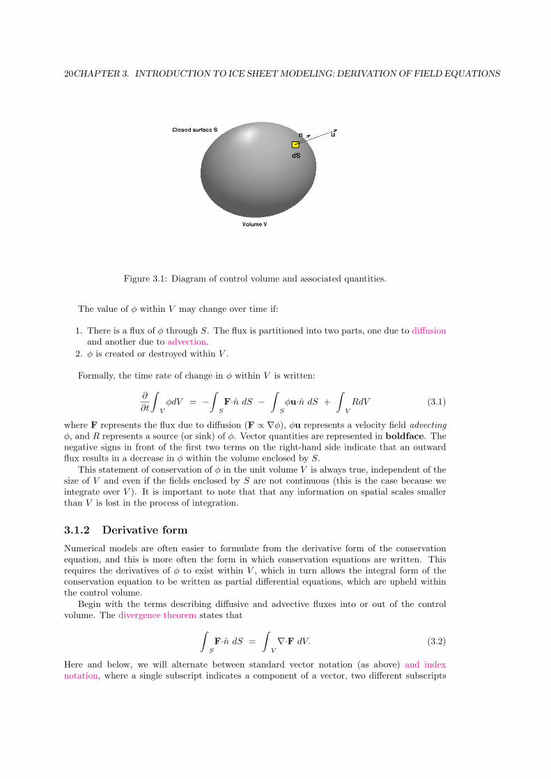
3.1.1 Integral form
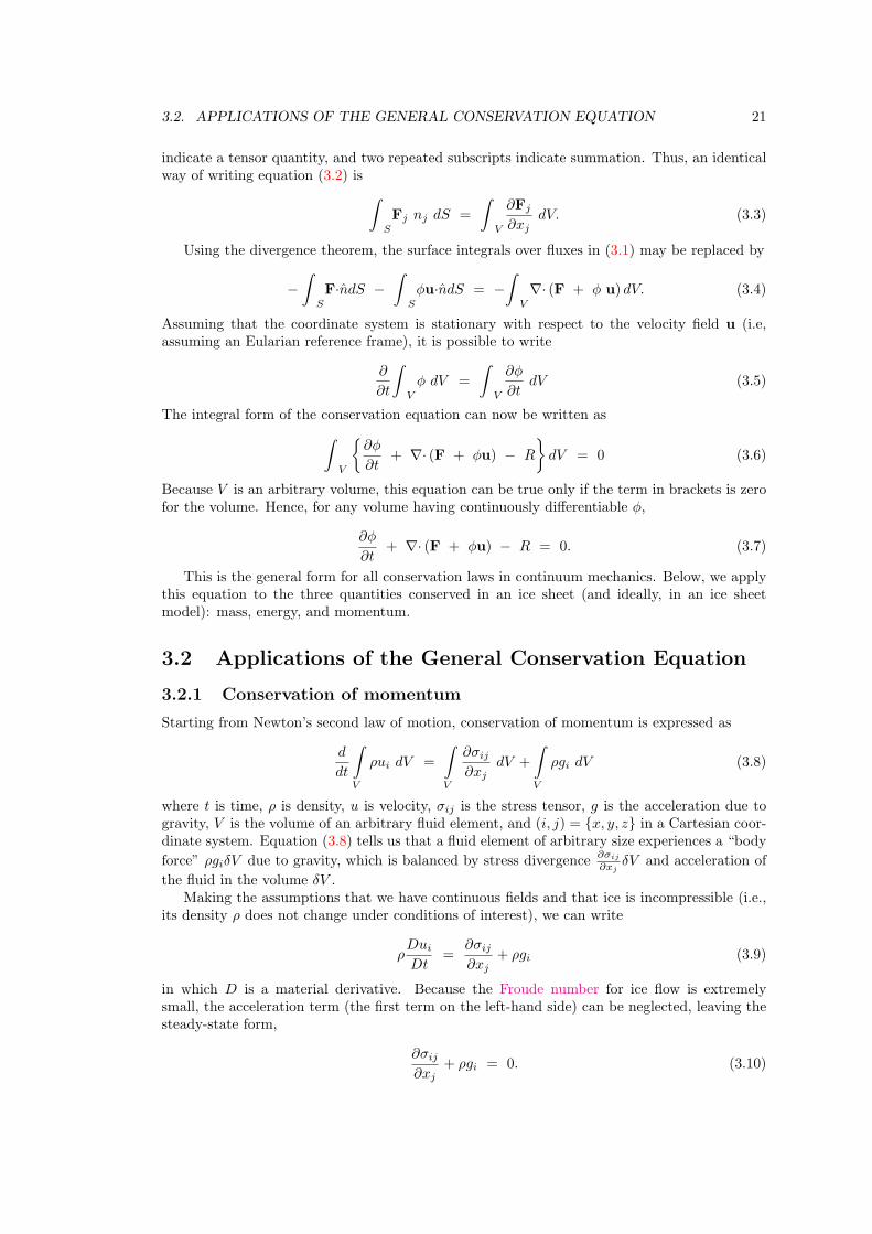
The mathematical formulation of conservation can be arrived at by considering the change ina quantity ϕ that is known within a control volume V . The control volume is enclosed by asurface S, with the outward positive unit vector n, normal to S.
19
20CHAPTER 3. INTRODUCTION TO ICE SHEETMODELING: DERIVATIONOF FIELD EQUATIONS
Figure 3.1: Diagram of control volume and associated quantities.
The value of ϕ within V may change over time if:
1. There is a flux of ϕ through S. The flux is partitioned into two parts, one due to diffusionand another due to advection.
2. ϕ is created or destroyed within V .
Formally, the time rate of change in ϕ within V is written:
∂
∂t
∫V
ϕdV = −∫
S
F·n dS −∫
S
ϕu·n dS +
∫V
RdV (3.1)
where F represents the flux due to diffusion (F ∝ ∇ϕ), ϕu represents a velocity field advectingϕ, and R represents a source (or sink) of ϕ. Vector quantities are represented in boldface. Thenegative signs in front of the first two terms on the right-hand side indicate that an outwardflux results in a decrease in ϕ within the volume enclosed by S.
This statement of conservation of ϕ in the unit volume V is always true, independent of thesize of V and even if the fields enclosed by S are not continuous (this is the case because weintegrate over V ). It is important to note that that any information on spatial scales smallerthan V is lost in the process of integration.
3.1.2 Derivative form
Numerical models are often easier to formulate from the derivative form of the conservationequation, and this is more often the form in which conservation equations are written. Thisrequires the derivatives of ϕ to exist within V , which in turn allows the integral form of theconservation equation to be written as partial differential equations, which are upheld withinthe control volume.
Begin with the terms describing diffusive and advective fluxes into or out of the controlvolume. The divergence theorem states that∫
S
F·n dS =
∫V
∇·F dV. (3.2)
Here and below, we will alternate between standard vector notation (as above) and indexnotation, where a single subscript indicates a component of a vector, two different subscripts
3.2. APPLICATIONS OF THE GENERAL CONSERVATION EQUATION 21
indicate a tensor quantity, and two repeated subscripts indicate summation. Thus, an identicalway of writing equation (3.2) is ∫
S
Fj nj dS =
∫V
∂Fj
∂xjdV. (3.3)
Using the divergence theorem, the surface integrals over fluxes in (3.1) may be replaced by
−∫
S
F·ndS −∫
S
ϕu·ndS = −∫
V
∇· (F + ϕ u) dV. (3.4)
Assuming that the coordinate system is stationary with respect to the velocity field u (i.e,assuming an Eularian reference frame), it is possible to write
∂
∂t
∫V
ϕ dV =
∫V
∂ϕ
∂tdV (3.5)
The integral form of the conservation equation can now be written as∫V
∂ϕ
∂t+ ∇· (F + ϕu) − R
dV = 0 (3.6)
Because V is an arbitrary volume, this equation can be true only if the term in brackets is zerofor the volume. Hence, for any volume having continuously differentiable ϕ,
∂ϕ
∂t+ ∇· (F + ϕu) − R = 0. (3.7)
This is the general form for all conservation laws in continuum mechanics. Below, we applythis equation to the three quantities conserved in an ice sheet (and ideally, in an ice sheetmodel): mass, energy, and momentum.
3.2 Applications of the General Conservation Equation
3.2.1 Conservation of momentum
Starting from Newton’s second law of motion, conservation of momentum is expressed as
d
dt
∫V
ρui dV =
∫V
∂σij
∂xjdV +
∫V
ρgi dV (3.8)
where t is time, ρ is density, u is velocity, σij is the stress tensor, g is the acceleration due togravity, V is the volume of an arbitrary fluid element, and (i, j) = x, y, z in a Cartesian coor-dinate system. Equation (3.8) tells us that a fluid element of arbitrary size experiences a “body
force” ρgiδV due to gravity, which is balanced by stress divergence∂σij
∂xjδV and acceleration of
the fluid in the volume δV .Making the assumptions that we have continuous fields and that ice is incompressible (i.e.,
its density ρ does not change under conditions of interest), we can write
ρDui
Dt=
∂σij
∂xj+ ρgi (3.9)
in which D is a material derivative. Because the Froude number for ice flow is extremelysmall, the acceleration term (the first term on the left-hand side) can be neglected, leaving thesteady-state form,
∂σij
∂xj+ ρgi = 0. (3.10)
22CHAPTER 3. INTRODUCTION TO ICE SHEETMODELING: DERIVATIONOF FIELD EQUATIONS
Equation (3.10) states that the body force (the gravitational driving force) is balanced byforces resulting from gradients in the stress tensor σij . All models of ice-flow dynamics arebased on solving this equation in some form. Chapters 4 and 6 provide additional details onthe approximations to this equation that are solved by CISM.
The stress tensor σij has nine components in a three-dimensional, Cartesian coordinatesystem,
σ =
∣∣∣∣∣∣σxx σxy σxz
σyx σyy σyz
σzx σzy σzz.
∣∣∣∣∣∣ (3.11)
Since σij is symmetric, only six of these components are independent. The components along thediagonal are called normal stresses, and the off-diagonal components are called shear stresses.Deformation results not from the full stress but from the deviatoric stress,
τij = σij − 1
3σkkδij , (3.12)
in which δij is the Kroneker delta (or the identity tensor). For shear stresses, (3.12) indicatesthat the full and deviatoric stresses are identical.
Constitutive relationship
To relate the stress tensor to fluid motion, we introduce the strain rate tensor,
ϵij =1
2
(∂ui
∂xj+
∂uj
∂xi
), i, j = x, y, z, (3.13)
where ui are the velocity vector components. The strain rate tensor ϵij , and hence gradients inthe velocity field, are related to the stress tensor τij by a constitutive relation. For a Newtonianfluid, this can be expressed as
τij = ηϵij , (3.14)
which states that the strain rate is proportional to the stress, with the ice viscosity η serving asthe constant of proportionality. Ice does not behave as a Newtonian fluid, and instead exhibitsa power-law rheology, so that it becomes more fluid (less viscous) the faster it deforms. Thisrelationship can be expressed through Nye’s generalization of Glen’s flow law,
τij = A(T ∗)−1n ϵ
1−nn
e ϵij (3.15)
in which T ∗ is the absolute temperature corrected for the pressure dependence of the melttemperature, ϵe is the second invariant (a norm) of the stress tensor, and the power-law exponentn is commonly taken as 3. A comparison of (3.14) and (3.15) indicates that one can define an“effective” ice viscosity for (3.14) as
ηe = A(T ∗)−1n ϵ
1−nn
e . (3.16)
The temperature-dependent rate factor A follows the Arrhenius relationship
A (T ∗) = EAoe−Q/RT∗
, (3.17)
in which Ao is a constant, Q is the activation energy for crystal creep, R is the gas constant,and E is a tuning parameter, which can be used to account for the effects of impurities andanisotropic ice fabrics. The homologous temperature is
T ∗ = T + ρgHΦ, (3.18)
in which Φ is 9.8 ×10⁻⁸ K Pa−1, or about 8.7 ×10⁻⁴ K m−1 in ice. The pressure-dependentmelt temperature is simply the triple point temperature minus the product ρgHΦ.
3.2. APPLICATIONS OF THE GENERAL CONSERVATION EQUATION 23
3.2.2 Conservation of energy
The first law of thermodynamics is used to make a basic statement of conservation of energy ina volume of ice V enclosed within a surface S:
d
dt
∫V
E dV = −∫S
F · n dS −∫S
Eu · n dS +
∫V
WdV (3.19)
in which E is the total energy within the volume, Fi is the energy flux due to diffusion, and Wrepresents any sources or sinks of energy within the volume. The term Eui is an energy fluxthrough S due to advection. Following the steps laid out earlier, we use the divergence theoremand the assumptions of continuous fields and incompressibility to obtain
dE
dt+ ∇ · (Fi + Eui) − W = 0 (3.20)
Our goal is to use the first law of thermodynamics to compute the temperature of the ice andany changes in that temperature over time.
The energy E is the product of density and the specific internal energy of the ice e, whichis itself the product of the specific heat capacity cp and temperature T (because there is notransfer between internal energy and pressure for an incompressible fluid). Thus,
dEdt = d(ρe)
dt
= ρdedt + edρ
dt
= ρcpdTdt
(3.21)
The heat flux due to diffusion follows Fourier’s “law” for heat conduction,
∇ · Fi = ∇ · (−k ∇T )= −k ∇2T,
(3.22)
in which k is the thermal conductivity of ice and we assume gradients in its magnitude to benegligible.
Using progress made above, we can write the advection term
∇ · (Eui) = ρcp ui · ∇T. (3.23)
In the expansion of the terms on the left-hand side of (3.23) (using the product rule), we haveimplicitly ignored the term involving ∇ · ui because it is small with respect to the other termsretained on the right-hand side.
Two energy sources must be considered: the work done on the system by internal deformationand the latent heat associated with phase changes. The former is the product of the strain rateand deviatoric stress, ϵijτij . The latter is the product of the latent heat of fusion and theamount of material (ice) subject to melting (or freezing) per unit volume, per unit time, LfMf .
At last, we can write equation (3.20) in terms of temperature:
∂T
∂t=
k
ρcp∇2T − ui · ∇T +
1
ρcpϵijτij +
1
ρcpLfMf . (3.24)
It is often the case that horizontal terms ∂2T∂x2 and ∂2T
∂y2 are small enough to be ignored.
3.2.3 Conservation of mass
In this case, ϕ from our general conservation equation represents the mass M , or more conve-niently M =
∫VρdV , the integral of the density over the volume. Assuming that there are no
sources or sinks of mass in the volume (R=0), the mass conservation equation is written
24CHAPTER 3. INTRODUCTION TO ICE SHEETMODELING: DERIVATIONOF FIELD EQUATIONS
∫V
∂ρ
∂tdV +
∫V
∇ · ρudV = 0 (3.25)
Ice is incompressible (the density does not change in time), which provides the equation forlocal mass continuity,
∇ · u = 0. (3.26)
Equation (3.26) says that the velocity field is divergence-free. Applying the ∇ operator inCartesian coordinates gives
∂ux
∂x+
∂uy
∂y+
∂uz
∂z= 0. (3.27)
To make use of this statement, we need to integrate from the base b to the upper surface s ofthe ice mass,
s∫b
(∂ux
∂x+
∂uy
∂y+
∂uz
∂z
)dz = 0. (3.28)
The integral of ∂uz
∂z is simply the difference between the vertical component of the velocity atthe upper and lower surfaces, so
uz (s)− uz (b) = −s∫
b
∂ux
∂xdz −
s∫b
∂uy
∂ydz. (3.29)
Changing the order of integration and differentiation using Leibniz’s rule, we obtain
uz (s)− uz (b) = − ∂∂x
∫ s
buxdz + ux(s)
∂s∂x − ux(b)
∂b∂x
− ∂∂y
∫ s
buydz + uy(s)
∂s∂y − uy(b)
∂b∂x .
(3.30)
The vertical velocity at the upper surface uz(s) is the result of motion parallel to the surfaceslope, the rate of new ice accumulation Bs, and any time change in the surface height,
uz (s) =∂s
∂t+ ux(s)
∂s
∂x+ uy(s)
∂s
∂y− Bs, (3.31)
recognizing that a negative accumulation rate indicates ablation. Similarly, the vertical velocityat the lower surface is
uz (b) =∂b
∂t+ ux(b)
∂b
∂x+ uy(b)
∂b
∂y− Mb (3.32)
in which Mb is the basal melt rate (Mb < 0 for freeze-on). Substituting (3.31) and (3.32) into(3.30), we find that many terms cancel:
∂s
∂t− Bs − ∂b
∂t+ Mb = − ∂
∂x
s∫b
uxdz − ∂
∂y
s∫b
uydz. (3.33)
Finally, making the substitution that the ice thickness H = s− b, we obtain
∂H
∂t= − ∂
∂x
s∫b
uxdz − ∂
∂y
s∫b
uydz + Bs − Mb. (3.34)
Integrating in the vertical gives
3.2. APPLICATIONS OF THE GENERAL CONSERVATION EQUATION 25
∂H
∂t= − ∇ · (UiH) + Bs − Mb, (3.35)
in which Ui is the vertically averaged velocity, i.e., Ui =1H
∫ s
buidz . Equation (3.35) is prog-
nostic; we can use the current velocity and geometry of the ice to compute the rate of changein the geometry.

26CHAPTER 3. INTRODUCTION TO ICE SHEETMODELING: DERIVATIONOF FIELD EQUATIONS
Chapter 4
Shallow Ice Dynamics: GlideDynamical Core
This chapter describes the numerical implementation of mass, momentum, and energy con-servation in the Glide dynamical core, which uses a Shallow Ice Approximation for ice flow.For a model governed by shallow-ice dynamics, the solutions for the conservation of mass andmomentum are intimately linked.
4.1 Ice Thickness Evolution
The evolution of the ice thickness, H, stems from the continuity equation and can be expressedas
∂H
∂t= −∇ · (uH) +B, (4.1)
where u is the vertically averaged ice velocity, B is the surface mass balance and ∇ is thehorizontal gradient operator (Payne and Dongelmans, 1997).
For some regions of large-scale ice sheets, such as the slow-moving interior, or for simulationsrun at coarse spatial resolution, a model governed by the shallow ice approximation (SIA) maybe appropriate. Further, for very long time integrations, such as those required in paleoclimatestudies, a model governed by the SIA may be the only computationally practical approach.
Based largely on the assumption that bedrock and ice surface slopes are sufficiently small(Hutter, 1983), the SIA neglects all stress components other than those associated with verticalshearing in the horizontal directions. These stresses, τxz and τyz, are approximated by
τxz(z) = −ρg(s− z)∂s
∂x,
τyz(z) = −ρg(s− z)∂s
∂y,
(4.2)
where ρ is the density of ice, g the acceleration due to gravity and s = H + b the ice surface.Strain rates ϵij of polycrystalline ice are related to the stress tensor by the nonlinear flow
law:
ϵiz =1
2
(∂ui
∂z+
∂uz
∂i
)= A(T ∗)τ
(n−1)∗ τiz i = x, y, (4.3)
where τ∗ is the effective shear stress defined by the second invariant of the stress tensor, n the flowlaw exponent and A the temperature–dependent flow law coefficient. T ∗ is the absolute temper-ature corrected for the dependence of the melting point on pressure (T ∗ = T +8.7 · 10−4(s− z),T in Kelvin, Huybrechts, 1986). The parameters n and A are determined experimentally; n
27
28 CHAPTER 4. SHALLOW ICE DYNAMICS: GLIDE DYNAMICAL CORE
is usually taken to be 3 and A depends primarily on temperature and secondarily on factorssuch as crystal size and orientation and ice impurities. Experiments suggest that A follows theArrhenius relationship:
A(T ∗) = fae−Q/RT∗, (4.4)
where a is a temperature–independent material constant, Q is the activation energy for creepand R is the universal gas constant (Paterson, 1994). The tuning parameter f may be usedto speed up the ice flow, accounting for the effects of ice impurities and the development ofanisotropic ice fabrics (Payne, 1999; Tarasov and Peltier, 1999, 2000; Peltier et al., 2000).
Integrating (4.4) with respect to z gives the vertical profile of the horizontal velocity in eachcolumn:
u(z)− u(b) = −2(ρg)n|∇s|n−1∇s
z∫b
A(s− z)ndz, (4.5)
where u(b) is the basal sliding velocity. Integrating (4.5) again with respect to z gives anexpression for the vertically averaged ice velocity:
uH = −2(ρg)n|∇s|n−1∇s
s∫b
z∫b
A(s− z)ndzdz′. (4.6)
The vertical ice velocity can be derived from the conservation of mass for an incompressiblematerial:
∂ux
∂x+
∂uy
∂y+
∂uz
∂z= 0. (4.7)
Integrating (4.7) with respect to z gives the vertical profile of the vertical velocity in eachcolumn:
w(z) = −z∫
h
∇ · u(z)dz + w(b), (4.8)
with lower kinematic boundary condition
w(b) =∂b
∂t+ u(b) ·∇b−Mb, (4.9)
where Mb is the basal melt rate given by (4.55). The upper kinematic boundary is given by thesurface mass balance and must satisfy
w(s) =∂s
∂t+ u(s) ·∇s−Bs. (4.10)
4.1.1 Numerical grid
The continuous equations describing ice physics have to be discretized in order to be solved bya computer (which is inherently finite). This section describes the finite–difference grids usedby the model.
Horizontal grid
The modelled region (x ∈ [0, Lx], y ∈ [0, Ly]) is discretized using a regular grid so that xi =(i− 1)∆x for i ∈ [1, N ] (and similarly for yj). The model uses two staggered horizontal grids inorder to improve stability. Both grids use the same grid spacing, ∆x and ∆y, but are offset byhalf a grid cell (see Fig. 4.1). Quantities calculated on the staggered (r, s)–grid are denoted with
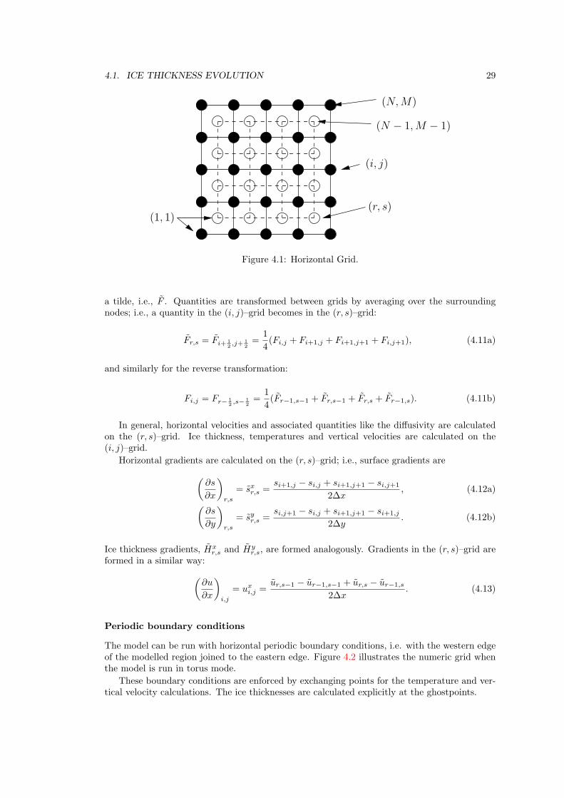
4.1. ICE THICKNESS EVOLUTION 29
(1, 1)
(N − 1,M − 1)
(r, s)
(i, j)
(N,M)
Figure 4.1: Horizontal Grid.
a tilde, i.e., F . Quantities are transformed between grids by averaging over the surroundingnodes; i.e., a quantity in the (i, j)–grid becomes in the (r, s)–grid:
Fr,s = Fi+ 12 ,j+
12=
1
4(Fi,j + Fi+1,j + Fi+1,j+1 + Fi,j+1), (4.11a)
and similarly for the reverse transformation:
Fi,j = Fr− 12 ,s−
12=
1
4(Fr−1,s−1 + Fr,s−1 + Fr,s + Fr−1,s). (4.11b)
In general, horizontal velocities and associated quantities like the diffusivity are calculatedon the (r, s)–grid. Ice thickness, temperatures and vertical velocities are calculated on the(i, j)–grid.
Horizontal gradients are calculated on the (r, s)–grid; i.e., surface gradients are(∂s
∂x
)r,s
= sxr,s =si+1,j − si,j + si+1,j+1 − si,j+1
2∆x, (4.12a)(
∂s
∂y
)r,s
= syr,s =si,j+1 − si,j + si+1,j+1 − si+1,j
2∆y. (4.12b)
Ice thickness gradients, Hxr,s and Hy
r,s, are formed analogously. Gradients in the (r, s)–grid areformed in a similar way:(
∂u
∂x
)i,j
= uxi,j =
ur,s−1 − ur−1,s−1 + ur,s − ur−1,s
2∆x. (4.13)
Periodic boundary conditions
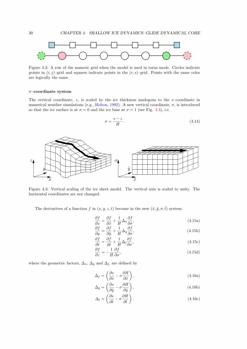
The model can be run with horizontal periodic boundary conditions, i.e. with the western edgeof the modelled region joined to the eastern edge. Figure 4.2 illustrates the numeric grid whenthe model is run in torus mode.
These boundary conditions are enforced by exchanging points for the temperature and ver-tical velocity calculations. The ice thicknesses are calculated explicitly at the ghostpoints.
30 CHAPTER 4. SHALLOW ICE DYNAMICS: GLIDE DYNAMICAL CORE
Figure 4.2: A row of the numeric grid when the model is used in torus mode. Circles indicatepoints in (i, j)–grid and squares indicate points in the (r, s)–grid. Points with the same colorare logically the same.
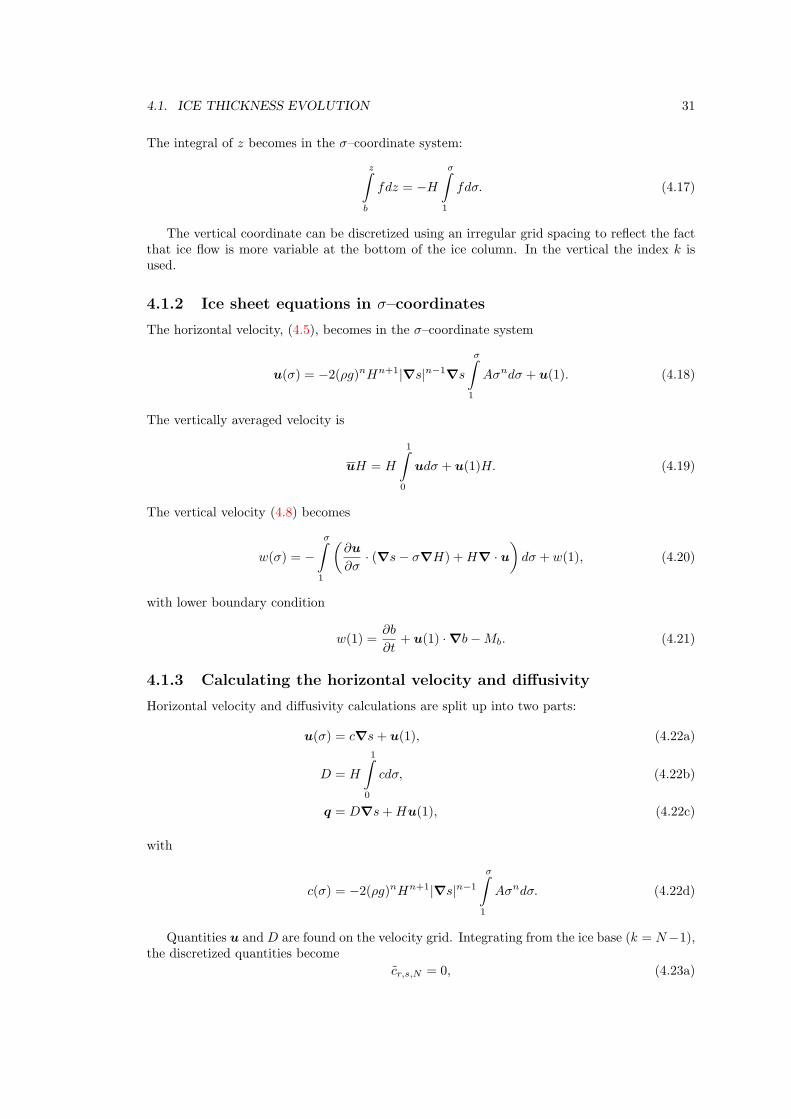
σ–coordinate system
The vertical coordinate, z, is scaled by the ice thickness analogous to the s–coordinate innumerical weather simulations (e.g., Holton, 1992). A new vertical coordinate, σ, is introducedso that the ice surface is at σ = 0 and the ice base at σ = 1 (see Fig. 4.3), i.e.
σ =s− z
H. (4.14)
y
x
z
y
x
σ
Figure 4.3: Vertical scaling of the ice sheet model. The vertical axis is scaled to unity. Thehorizontal coordinates are not changed.
The derivatives of a function f in (x, y, z, t) become in the new (x, y, σ, t) system:
∂f
∂x=
∂f
∂x+
1
H∆x
∂f
∂σ, (4.15a)
∂f
∂y=
∂f
∂y+
1
H∆y
∂f
∂σ, (4.15b)
∂f
∂t=
∂f
∂t+
1
H∆t
∂f
∂σ, (4.15c)
∂f
∂z= − 1
H
∂f
∂σ, (4.15d)
where the geometric factors, ∆x, ∆y and ∆t, are defined by
∆x =
(∂s
∂x− σ
∂H
∂x
), (4.16a)
∆y =
(∂s
∂y− σ
∂H
∂y
), (4.16b)
∆t =
(∂s
∂t− σ
∂H
∂t
). (4.16c)
4.1. ICE THICKNESS EVOLUTION 31
The integral of z becomes in the σ–coordinate system:
z∫b
fdz = −H
σ∫1
fdσ. (4.17)
The vertical coordinate can be discretized using an irregular grid spacing to reflect the factthat ice flow is more variable at the bottom of the ice column. In the vertical the index k isused.
4.1.2 Ice sheet equations in σ–coordinates
The horizontal velocity, (4.5), becomes in the σ–coordinate system
u(σ) = −2(ρg)nHn+1|∇s|n−1∇s
σ∫1
Aσndσ + u(1). (4.18)
The vertically averaged velocity is
uH = H
1∫0
udσ + u(1)H. (4.19)
The vertical velocity (4.8) becomes
w(σ) = −σ∫
1
(∂u
∂σ· (∇s− σ∇H) +H∇ · u
)dσ + w(1), (4.20)
with lower boundary condition
w(1) =∂b
∂t+ u(1) ·∇b−Mb. (4.21)
4.1.3 Calculating the horizontal velocity and diffusivity
Horizontal velocity and diffusivity calculations are split up into two parts:
u(σ) = c∇s+ u(1), (4.22a)
D = H
1∫0
cdσ, (4.22b)
q = D∇s+Hu(1), (4.22c)
with
c(σ) = −2(ρg)nHn+1|∇s|n−1
σ∫1
Aσndσ. (4.22d)
Quantities u and D are found on the velocity grid. Integrating from the ice base (k = N−1),the discretized quantities become
cr,s,N = 0, (4.23a)
32 CHAPTER 4. SHALLOW ICE DYNAMICS: GLIDE DYNAMICAL CORE
cr,s,k = −2(ρg)nHn+1r,s
((sxr,s)
2 + (syr,s)2)n−1
2
k∑κ=N−1
Ar,s,κ +Ar,s,κ+1
2
(σκ+1 + σκ
2
)n
(σκ+1 − σκ), (4.23b)
Dr,s = Hr,s
N−1∑k=0
cr,s,k + cr,s,k+1
2(σk+1 − σk). (4.23c)
Expressions for ui,j,k and qi,j are straightforward.
4.1.4 Solving the ice thickness evolution equation
Equation (4.1) can be rewritten as a diffusion equation, with nonlinear diffusion coefficient D:
∂H
∂t= −∇ ·D∇s+B = −∇ · q +B, (4.24)
where B = Bs − Mb is the total mass balance. This nonlinear partial differential equationcan be linearized by using the diffusion coefficient from the previous time step. The diffusioncoefficient is calculated on the (r, s)–grid, i.e. staggered in both x and y directions. Figure 4.4illustrates the staggered grid. Using finite differences, the fluxes in the x direction, qx, become
qxi+ 12 ,j
= −1
2(Dr,s + Dr,s−1)
si+1,j − si,j∆x
, (4.25a)
qxi− 12 ,j
= −1
2(Dr−1,s + Dr−1,s−1)
si,j − si−1,j
∆x, (4.25b)
and the fluxes in the y direction are
qyi,j+ 1
2
= −1
2(Dr,s + Dr−1,s)
si,j+1 − si,j∆y
, (4.25c)
qyi,j− 1
2
= −1
2(Dr,s−1 + Dr−1,s−1)
si,j − si,j−1
∆y. (4.25d)
ADI Scheme
The alternating–direction implicit (ADI) method uses the concept of operator splitting where(4.24) is solved first in the x–direction and then in the y–direction (Press et al., 1992). Thetime step ∆t is divided into two partial steps ∆t/2. The discretized version of Equation (4.24)becomes (Huybrechts, 1986):
2H
t+ 12
i,j −Hti,j
∆t= −
qx,t+ 1
2
i+ 12 ,j
− qx,t+ 1
2
i− 12 ,j
∆x−
qy,ti,j+ 1
2
− qy,ti,j− 1
2
∆y+Bi,j , (4.26a)
2Ht+1
i,j −Ht+ 1
2i,j
∆t= −
qx,t+ 1
2
i+ 12 ,j
− qx,t+ 1
2
i− 12 ,j
∆x−
qy,t+1
i,j+ 12
− qy,t+1
i,j− 12
∆y+Bi,j . (4.26b)
Gathering all t+ 12 terms on the left side,(4.26a) can be expressed as a tridiagonal set of equations
for each row j:
− αi,jHt+ 1
2i−1,j + (1− βi,j)H
t+ 12
i,j − γi,jHt+ 1
2i+1,j = δi,j , (4.27)
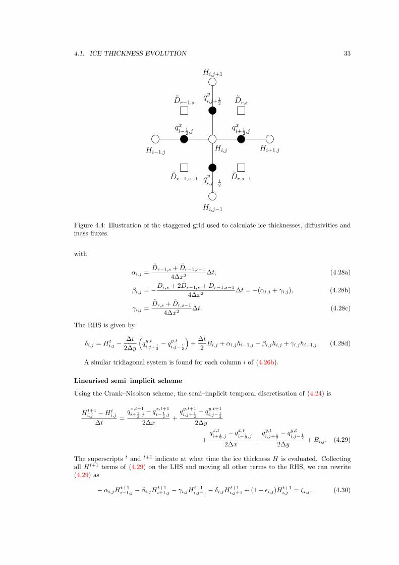
4.1. ICE THICKNESS EVOLUTION 33
Dr−1,s
Hi−1,jHi+1,j
Hi,j+1
Hi,j−1
Hi,j
qxi− 1
2,j
qxi+ 1
2,j
qy
i,j+ 1
2
qy
i,j− 1
2
Dr−1,s−1 Dr,s−1
Dr,s
Figure 4.4: Illustration of the staggered grid used to calculate ice thicknesses, diffusivities andmass fluxes.
with
αi,j =Dr−1,s + Dr−1,s−1
4∆x2∆t, (4.28a)
βi,j = −Dr,s + 2Dr−1,s + Dr−1,s−1
4∆x2∆t = −(αi,j + γi,j), (4.28b)
γi,j =Dr,s + Dr,s−1
4∆x2∆t. (4.28c)
The RHS is given by
δi,j = Hti,j −
∆t
2∆y
(qy,ti,j+ 1
2
− qy,ti,j− 1
2
)+
∆t
2Bi,j + αi,jhi−1,j − βi,jhi,j + γi,jhi+1,j . (4.28d)
A similar tridiagonal system is found for each column i of (4.26b).
Linearised semi–implicit scheme
Using the Crank–Nicolson scheme, the semi–implicit temporal discretisation of (4.24) is
Ht+1i,j −Ht
i,j
∆t=
qx,t+1
i+ 12 ,j
− qx,t+1
i− 12 ,j
2∆x+
qy,t+1
i,j+ 12
− qy,t+1
i,j− 12
2∆y
+qx,ti+ 1
2 ,j− qx,t
i− 12 ,j
2∆x+
qy,ti,j+ 1
2
− qy,ti,j− 1
2
2∆y+Bi,j . (4.29)
The superscripts t and t+1 indicate at what time the ice thickness H is evaluated. Collectingall Ht+1 terms of (4.29) on the LHS and moving all other terms to the RHS, we can rewrite(4.29) as
− αi,jHt+1i−1,j − βi,jH
t+1i+1,j − γi,jH
t+1i,j−1 − δi,jH
t+1i,j+1 + (1− ϵi,j)H
t+1i,j = ζi,j , (4.30)
34 CHAPTER 4. SHALLOW ICE DYNAMICS: GLIDE DYNAMICAL CORE
with the RHS
ζi,j = αi,jHti−1,j + βi,jH
ti+1,j + γi,jH
ti,j−1 + δi,jH
ti,j+1 + (1 + ϵi,j)H
ti,j
+ 2(αi,jhi−1,j + βi,jhi+1,j + γi,jhi,j−1 + δi,jhi,j+1 + ϵi,jhi,j) +Bi,j∆t. (4.31)
Here the elements of the sparse matrix are
αi,j =Dr−1,s + Dr−1,s−1
4∆x2∆t, (4.32a)
βi,j =Dr,s + Dr,s−1
4∆x2∆t, (4.32b)
γi,j =Dr,s−1 + Dr−1,s−1
4∆y2∆t, (4.32c)
δi,j =Dr,s + Dr−1,s
4∆y2∆t, (4.32d)
ϵi,j = −(αi,j + βi,j + γi,j + δi,j). (4.32e)
This matrix equation is solved using an iterative solver for non-symmetric sparse matrices.The solver used here is the bi–conjugate gradient method with incomplete LU decompositionpreconditioning provided by the SLAP package.
Nonlinear scheme
The nonlinearity of (4.24) arises from the dependance of D on s. A nonlinear scheme for (4.24)can be formulated using Picard iteration, which consists of two iterations: an outer, nonlinearand an inner, linear equation. The scheme starts with the diffusivity from the previous timestep:
D(0),t+1 = Dt. (4.33a)
Equation (4.30) becomes
− α(ξ),t+1i,j Ht+1
i−1,j − β(ξ),t+1i,j H
(ξ+1),t+1i+1,j − γ
(ξ),t+1i,j H
(ξ+1),t+1i,j−1
− δ(ξ),t+1i,j H
(ξ+1),t+1i,j+1 + (1− ϵ
(ξ),t+1i,j )H
(ξ+1),t+1i,j = ζ
(0),ti,j . (4.33b)
Equation (4.33b) is iterated over ξ until the maximum ice thickness residual is smaller thansome threshold:
max(∣∣∣H(ξ+1),t+1 −H(ξ),t+1
∣∣∣) < Hres. (4.34)
4.1.5 Calculating vertical velocities
Grid velocity
The vertical grid moves as a result of using a σ–coordinate system. The grid velocity is
wgrid(σ) =∂s
∂t+ u ·∇s− σ
(∂H
∂t+ u ·∇H
). (4.35)
The numerical implementation of (4.35) is straightforward.
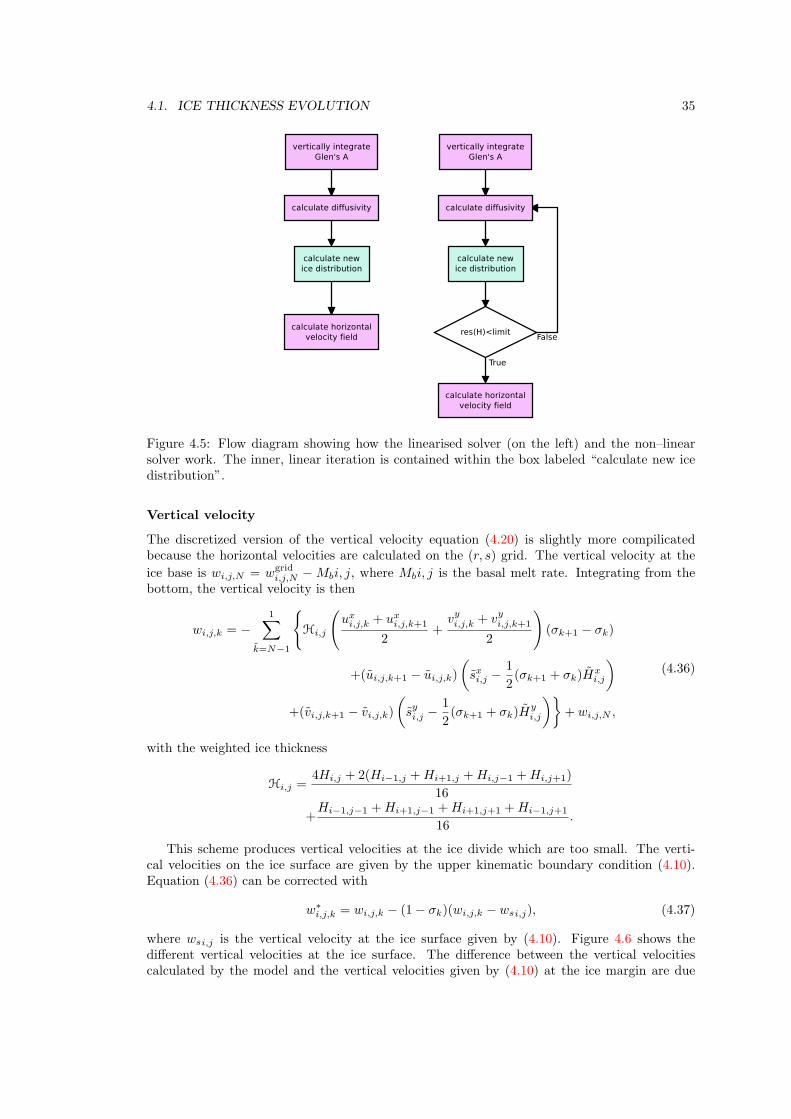
4.1. ICE THICKNESS EVOLUTION 35
Figure 4.5: Flow diagram showing how the linearised solver (on the left) and the non–linearsolver work. The inner, linear iteration is contained within the box labeled “calculate new icedistribution”.
Vertical velocity
The discretized version of the vertical velocity equation (4.20) is slightly more compilicatedbecause the horizontal velocities are calculated on the (r, s) grid. The vertical velocity at the
ice base is wi,j,N = wgridi,j,N − Mbi, j, where Mbi, j is the basal melt rate. Integrating from the
bottom, the vertical velocity is then
wi,j,k = −1∑
k=N−1
Hi,j
(uxi,j,k + ux
i,j,k+1
2+
vyi,j,k + vyi,j,k+1
2
)(σk+1 − σk)
+(ui,j,k+1 − ui,j,k)
(sxi,j −
1
2(σk+1 + σk)H
xi,j
)+(vi,j,k+1 − vi,j,k)
(syi,j −
1
2(σk+1 + σk)H
yi,j
)+ wi,j,N ,
(4.36)
with the weighted ice thickness
Hi,j =4Hi,j + 2(Hi−1,j +Hi+1,j +Hi,j−1 +Hi,j+1)
16
+Hi−1,j−1 +Hi+1,j−1 +Hi+1,j+1 +Hi−1,j+1
16.
This scheme produces vertical velocities at the ice divide which are too small. The verti-cal velocities on the ice surface are given by the upper kinematic boundary condition (4.10).Equation (4.36) can be corrected with
w∗i,j,k = wi,j,k − (1− σk)(wi,j,k − wsi,j), (4.37)
where wsi,j is the vertical velocity at the ice surface given by (4.10). Figure 4.6 shows thedifferent vertical velocities at the ice surface. The difference between the vertical velocitiescalculated by the model and the vertical velocities given by (4.10) at the ice margin are due
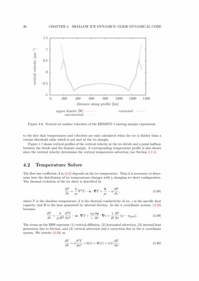
36 CHAPTER 4. SHALLOW ICE DYNAMICS: GLIDE DYNAMICAL CORE
-1
-0.5
0
0.5
1
1.5
0 200 400 600 800 1000 1200 1400
vertical
velocity
[ma−
1]
distance along profile [km]
upper kinetic BCuncorrected
corrected
Figure 4.6: Vertical ice surface velocities of the EISMINT-1 moving margin experiment.
to the fact that temperatures and velocities are only calculated when the ice is thicker than acertain threshold value which is not met at the ice margin.
Figure 4.7 shows vertical profiles of the vertical velocity at the ice divide and a point halfwaybetween the divide and the domain margin. A corresponding temperature profile is also shownsince the vertical velocity determines the vertical temperature advection (see Section 4.2.4).
4.2 Temperature Solver
The flow law coefficient A in (4.3) depends on the ice temperature. Thus it is necessary to deter-mine how the distribution of ice temperatures changes with a changing ice sheet configuration.The thermal evolution of the ice sheet is described by
∂T
∂t=
k
ρc∇2T − u ·∇T +
Φ
ρc− w
∂T
∂z, (4.38)
where T is the absolute temperature, k is the thermal conductivity of ice, c is the specific heatcapacity, and Φ is the heat generated by internal friction. In the σ–coordinate system, (4.38)becomes
∂T
∂t=
k
ρcH2
∂2T
∂σ2− u ·∇T +
σg
c
∂u
∂σ·∇s+
1
H
∂T
∂σ(w − wgrid) . (4.39)
The terms on the RHS represent (1) vertical diffusion, (2) horizontal advection, (3) internal heatgeneration due to friction, and (4) vertical advection and a correction due to the σ–coordinatesystem. We rewrite (4.39) as
∂T
∂t= a
∂2T
∂σ2+ b(σ) + Φ(σ) + c(σ)
∂T
∂σ, (4.40)
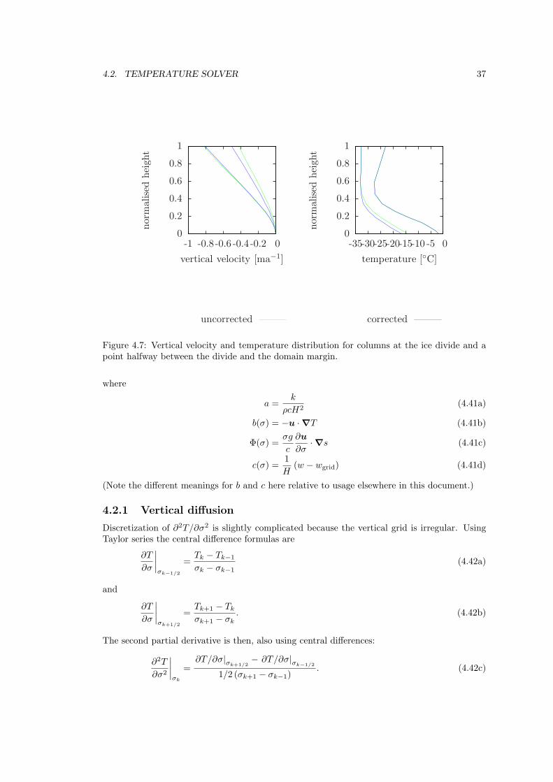
4.2. TEMPERATURE SOLVER 37
0
0.2
0.4
0.6
0.8
1
-1 -0.8 -0.6 -0.4 -0.2 0
normalised
heigh
t
vertical velocity [ma−1]
0
0.2
0.4
0.6
0.8
1
-35-30-25-20-15-10 -5 0
normalised
heigh
t
temperature [C]
uncorrected corrected
Figure 4.7: Vertical velocity and temperature distribution for columns at the ice divide and apoint halfway between the divide and the domain margin.
where
a =k
ρcH2(4.41a)
b(σ) = −u ·∇T (4.41b)
Φ(σ) =σg
c
∂u
∂σ·∇s (4.41c)
c(σ) =1
H(w − wgrid) (4.41d)
(Note the different meanings for b and c here relative to usage elsewhere in this document.)
4.2.1 Vertical diffusion
Discretization of ∂2T/∂σ2 is slightly complicated because the vertical grid is irregular. UsingTaylor series the central difference formulas are
∂T
∂σ
∣∣∣∣σk−1/2
=Tk − Tk−1
σk − σk−1(4.42a)
and
∂T
∂σ
∣∣∣∣σk+1/2
=Tk+1 − Tk
σk+1 − σk. (4.42b)
The second partial derivative is then, also using central differences:
∂2T
∂σ2
∣∣∣∣σk
=∂T/∂σ|σk+1/2
− ∂T/∂σ|σk−1/2
1/2 (σk+1 − σk−1). (4.42c)
38 CHAPTER 4. SHALLOW ICE DYNAMICS: GLIDE DYNAMICAL CORE
Inserting (4.42a) and (4.42b) into (4.42c), we obtain
∂2T
∂σ2
∣∣∣∣σk
=2(Tk+1 − Tk)
(σk+1 − σk)(σk+1 − σk−1)− 2(Tk − Tk−1)
(σk − σk−1)(σk+1 − σk−1). (4.42d)
Finally, the terms of equation (4.42d) are rearranged:
∂2T
∂σ2
∣∣∣∣σk
=2Tk−1
(σk − σk−1)(σk+1 − σk−1)− 2Tk
(σk+1 − σk)(σk − σk−1)
+2Tk+1
(σk+1 − σk)(σk+1 − σk−1). (4.43)
4.2.2 Horizontal advection
The horizontal advection term, −u ·∇T , is found using an upwinding scheme. We start withthe 1D case. (The method can readily be extended to 2D.) As always, the temperature functionis expressed as a Taylor series:
T (x+∆x) = T (x) + ∆xT ′(x) +∆x2
2T ′′(x) + . . . (4.44a)
If we replace ∆x with 2∆x, (4.44a) becomes
T (x+ 2∆x) = T (x) + 2∆xT ′(x) + 2∆x2T ′′(x) + . . . (4.44b)
From (4.44a) and (4.44b) we can construct a difference formula where the O(∆x2) error iscancelled, by multiplying (4.44a) with 4 and substracting the result from (4.44b):
T ′+(x) =
4T (x+∆x)− T (x+ 2∆x)− 3T (x)
2∆x, (4.45a)
and similarly for the backward difference:
T ′−(x) = −4T (x−∆x)− T (x− 2∆x)− 3T (x)
2∆x. (4.45b)
So the horizontal advection term in 1D becomes
bx = −ux∂T
∂x=
−ux
2∆x
−(4Ti−1 − Ti−2 − 3Ti) when ux > 0
4Ti+1 − Ti+2 − 3Ti when ux < 0(4.46)
A similar expression is found for by by substituting y for x. The combined horizontal advectionterm is
b = −u ·∇T = −(ux
∂T
∂x+ uy
∂T
∂y
)= bx + by = b1 + b2Ti. (4.47)
4.2.3 Heat generation
Taking the derivative of (4.18) with respect to σ, we get
∂ux
∂σ= −2(ρg)nHn+1|∇s|n−1 ∂s
∂xA(T ∗)σn. (4.48)
4.2. TEMPERATURE SOLVER 39
Thus,
Φ(σ) =σg
c
∂u
∂σ·∇s =
σg
c
(∂ux
∂σ
∂s
∂x+
∂uy
∂σ
∂s
∂y
)= −2(ρg)nHn+1|∇s|n−1σg
cA(T ∗)σn
((∂s
∂x
)2
+
(∂s
∂y
)2)
= − 2
cρ(gσρ)n+1 (H|∇s|)n+1
A(T ∗).
(4.49)
The constant factor 2cρ (gσρ)
n+1 is calculated during initialization in the subroutine glide init temp.This factor is assigned to array c1(1:upn). c1 also includes various scaling factors and the factor1/16 to normalise A.
The factor (H|∇s|)n+1is calculated in subroutine glide finddisp:
c2i,j =
(Hi,j
√Sx
2
i,j + Sy2
i,j
)n+1
. (4.50)
The final factor is found by averaging over the neighboring nodes:
Ai,j = 4Ai,j+2(Ai−1,j+Ai+1,j+Ai,j−1+Ai,j+1)+(Ai−1,j−1+Ai+1,j−1+Ai+1,j+1+Ai−1,j+1).(4.51)
4.2.4 Vertical advection
The vertical advection term ∂T/∂σ is computed from the central difference formula for unevenlyspaced nodes:
∂T
∂σ=
Tk+1 − Tk−1
σk+1 − σk−1. (4.52)
4.2.5 Boundary conditions
At the upper boundary, ice temperatures are set to the surface temperature, Tsurf. The ice atthe base is heated by the geothermal heat flux and sliding friction:
∂T
∂σ
∣∣∣∣σ=1
= −GH
k− Hτ b · u(1)
k, (4.53)
where τ b = −ρgH∇s is the basal shear stress and u(1) is the basal ice velocity. Ice temperaturesare held constant if they reach the pressure melting point of ice, i.e.
T ∗ = Tpmp if T ≥ Tpmp. (4.54)
Excess heat is then used to formulate a melt rate, Mb:
Mb =k
ρL
(∂T ∗
∂z− ∂T
∂z
), (4.55)
where L is the latent heat of fusion. Finally, basal temperatures are held constant if the ice isfloating:
∂T (1)
∂t= 0. (4.56)
40 CHAPTER 4. SHALLOW ICE DYNAMICS: GLIDE DYNAMICAL CORE
4.2.6 Putting it all together
Equation (4.39) is solved for each ice column. The horizontal dependency of the horizontaladvection term, (4.41b), is resolved by iterating the vertical solution. Combining the individualterms using a fully explicit finite-difference scheme, (4.40) becomes
Tk,t+1 − Tk,t
∆t=
(2aTk−1,t
(σk − σk−1)(σk+1 − σk−1)− 2aTk,t
(σk+1 − σk)(σk − σk−1,t)
+2aTk+1,t
(σk+1 − σk)(σk+1 − σk−1)
)+ b1k,t + b2kTk,t +Φk + ck
Tk+1,t − Tk−1,t
σk+1 − σk−1. (4.57a)
Similarly, the fully implicit scheme is
Tk,t+1 − Tk,t
∆t=
(2aTk−1,t+1
(σk − σk−1)(σk+1 − σk−1)− 2aTk,t+1
(σk+1 − σk)(σk − σk−1,t+1)
+2aTk+1,t+1
(σk+1 − σk)(σk+1 − σk−1)
)+ b1k,t+1 + b2kTk,t+1 +Φk + ck
Tk+1,t+1 − Tk−1,t+1
σk+1 − σk−1. (4.57b)
Taking the average of (4.57a) and (4.57b) gives the Crank–Nicolson scheme. The resultingequation is then rearranged, with terms of Tk−1,t+1, Tk,t+1 and Tk+1,t+1 combined to give thetridiagonal system
αkTk−1,t+1 + βkTk,t+1 + γkTk+1,t+1 = δk, (4.58)
where for k = 2 to N − 1 we have
αk = −1
2
2a∆t
(σk − σk−1)(σk+1 − σk−1)+
1
2
ck∆t
σk+1 − σk−1, (4.59a)
βk = 1 +1
2
2a∆t
(σk+1 − σk)(σk − σk−1)− 1
2b2k∆t = 1− αk − γk − 1
2b2k∆t, (4.59b)
γk = −1
2
2a∆t
(σk+1 − σk)(σk+1 − σk−1)− 1
2
ck∆t
σk+1 − σk−1, (4.59c)
δk = −αkTk−1,t + (2− βk)Tk,t − γkTk+1,t +1
2(b1k,t + b1k,t+1)∆t+Φk∆t. (4.59d)
Boundary conditions
At the upper boundary we have
α1 = 0, β1 = 1, γ1 = 0, δ1 = Tsurf. (4.59e)
The lower boundary condition is more complicated. Here we consider only the case when thetemperature is below the pressure melting point of ice. The BCs for floating ice and temperaturesat the pressure melting point of ice are trivial. The geothermal heat flux is applied at the lowerboundary; i.e., (4.42b) becomes
∂T
∂σ
∣∣∣∣σk+1/2
= −GH
k. (4.60)
Assuming that σk − σk−1 = σk+1 − σk = ∆σ and inserting (4.42a) and (4.60) into (4.42c), thesecond partial derivative becomes
∂2T
∂σ2
∣∣∣∣σN
=
(−GH
k− TN − TN−1
∆σ
)/∆σ = − GH
k∆σ− TN − TN−1
∆σ2. (4.61)
Inserting the new conduction term and replacing the derivative of the vertical advection termwith the Neumann boundary condition, (4.57a) becomes
TN,t+1 − TN,t
∆t= −a
(GH
k∆σ+
TN,t − TN−1,t
∆σ2
)+ b1N,t + b2NTN,t +ΦN − cN
GH
k, (4.62a)
4.3. BASAL BOUNDARY CONDITION 41
and similarly for (4.57b):
TN,t+1 − TN,t
∆t= −a
(GH
k∆σ+
TN,t+1 − TN−1,t+1
∆σ2
)+ b1N,t+1 + b2NTN,t+1
+ΦN − cNGH
k. (4.62b)
The elements of the tridiagonal system at the lower boundary are then
αN = − a∆t
2(σN − σN−1)2, (4.63a)
βN = 1− αN +1
2b2N∆t, (4.63b)
γN = 0, (4.63c)
δN =− αNTN−1,t + (2− βN )TN,t − aGH∆t
k(σN − σN−1)
+1
2(b1N,t + b1N,t+1)∆t+ΦN∆t− cN
GH∆t
k.
(4.63d)
4.3 Basal Boundary Condition
This section describes the formulation of the basal boundary condition. An interface for theupper boundary condition (atmospheric BC) is easily defined by the surface temperature andmass balance. Similarly, the basal boundary consists of mechanical and thermal boundaryconditions. The complications arise because the thermal and mechanical boundary conditionsdepend on each other. The interface of the basal boundary can be described with the followingfields (see also Fig. 4.8):
1. basal traction: This field specifies a parameter which is used to allow basal sliding.
2. basal heat flux: This is the heat flux entering the ice sheet from below.
3. basal water depth: The presence of basal melt water affects the basal ice temperature.
Also, the ice sheet model calculates a melt/freeze rate based on the temperature gradient andbasal water depth. This is handled by Glide.
4.3.1 Mechanical boundary conditions
If the ice is not frozen to the bed, basal decollement may occur. This can be parameterizedby a traction factor, tb. Within the ice sheet model, tb can be used to calculate basal slidingvelocities ub in the case of zero–order physics. That is,
ub = tbτ b, (4.64)
where τb is the basal shear stress. Alternatively, tb can be used as part of the stress–balancecalculations when the model is used with higher order physics. In simple models tb may beuniform or prescribed as a spatial variable. More complex models may wish to make tb dependenton other variables, such as basal melt rate. Typically tb will depend on the presence of basalwater.
The second mechanical boundary condition, basal melting/freeze–on Mb, is handled withinthe ice sheet model. The details are described in Section 4.3.2.
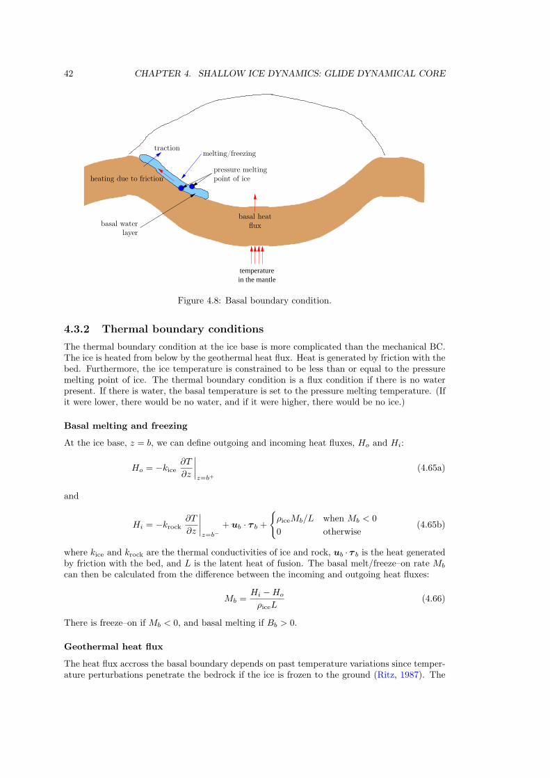
42 CHAPTER 4. SHALLOW ICE DYNAMICS: GLIDE DYNAMICAL CORE
temperaturein the mantle
fluxbasal waterlayer
melting/freezingtraction
pressure meltingheating due to friction point of ice
basal heat
Figure 4.8: Basal boundary condition.
4.3.2 Thermal boundary conditions
The thermal boundary condition at the ice base is more complicated than the mechanical BC.The ice is heated from below by the geothermal heat flux. Heat is generated by friction with thebed. Furthermore, the ice temperature is constrained to be less than or equal to the pressuremelting point of ice. The thermal boundary condition is a flux condition if there is no waterpresent. If there is water, the basal temperature is set to the pressure melting temperature. (Ifit were lower, there would be no water, and if it were higher, there would be no ice.)
Basal melting and freezing
At the ice base, z = b, we can define outgoing and incoming heat fluxes, Ho and Hi:
Ho = −kice∂T
∂z
∣∣∣∣z=b+
(4.65a)
and
Hi = −krock∂T
∂z
∣∣∣∣z=b−
+ ub · τ b +
ρiceMb/L when Mb < 0
0 otherwise(4.65b)
where kice and krock are the thermal conductivities of ice and rock, ub · τ b is the heat generatedby friction with the bed, and L is the latent heat of fusion. The basal melt/freeze–on rate Mb
can then be calculated from the difference between the incoming and outgoing heat fluxes:
Mb =Hi −Ho
ρiceL(4.66)
There is freeze–on if Mb < 0, and basal melting if Bb > 0.
Geothermal heat flux
The heat flux accross the basal boundary depends on past temperature variations since temper-ature perturbations penetrate the bedrock if the ice is frozen to the ground (Ritz, 1987). The
4.3. BASAL BOUNDARY CONDITION 43
heat equation for the bedrock layer is given by the diffusion equation
∂T
∂t=
krockρrockcrock
∇2T =krock
ρrockcrock
(∂2T
∂x2+
∂2T
∂y2+
∂2T
∂z2
), (4.67)
where krock is the thermal conductivity, ρrock the density, and crock the specific heat capacity ofthe bedrock layer.
Initial conditions for the temperature field T are found by applying the geothermal heat fluxG to an arbitrary surface temperature T0:
T (x, y, z) = T0 +G
krockz. (4.68)
This ensures that initially the geothermal heat flux experienced by the ice sheet is equal to theregional heat flux. The basal boundary condition of the bedrock layer is kept constant, i.e.
T (x, y,Hrock) = T0 +G
krockHrock. (4.69)
Lateral boundary conditions are given by
∂T
∂x
∣∣∣∣x=0
=∂T
∂x
∣∣∣∣x=Lx
=∂T
∂y
∣∣∣∣y=0
=∂T
∂y
∣∣∣∣y=Ly
= 0. (4.70)
At the upper boundary, the heat flux of the rock layer has to be matched with the heat flux inthe basal ice layer when the ice is frozen to the bed, i.e.
krock∂T
∂z
∣∣∣∣z=−0
= kice∂T
∂z
∣∣∣∣z=+0
. (4.71)
Otherwise the temperature of the top bedrock layer is set to the surface temperature (if thecell has been occupied by ice, but there is no ice present) or the basal ice temperature (if thereis ice). Equation (4.71) is automatically fulfilled if we set the top bedrock temperature to thebasal ice temperature everywhere and then calculate the geothermal heat flux to be used asboundary condition for (4.38).
4.3.3 Numerical solution
The horizontal grid of the bedrock layer is described in Section 4.1.1. The vertical bedrockgrid is irregular like the vertical grid of the ice sheet. However, it is not scaled. Also for now,we ignore topography or isostatic adjustment, i.e. the bedrock layer is assumed to be flat andconstant.
The horizontal second derivative in (4.67) becomes using finite–differences
∂2T
∂x2
∣∣∣∣xi,yi,zi
= Txx,i,j,k =Ti+1,j,k − 2Ti,j,k + Ti−1,j,k
∆x, (4.72)
and similarly for ∂2T/∂y2. The vertical second derivative ∂2T/∂z2 is similar to (4.43):
∂2T
∂z2
∣∣∣∣xi,yi,zi
= Tzz,i,j,k =2Ti,j,k−1
(zk − zk−1)(zk+1 − zk−1)− 2Ti,j,k
(zk+1 − zk)(zk − zk−1)
+2Ti,j,k+1
(zk+1 − zk)(zk+1 − zk−1). (4.73)
Using the Crank-Nicholson scheme, (4.67) becomes
T t+1i,j,k − T t
i,j,k
∆t= D
T t+1xx,i,j,k + T t
xx,i,j,k
2+
T t+1yy,i,j,k + T t
yy,i,j,k
2+
T t+1zz,i,j,k + T t
zz,i,j,k
2
, (4.74)
44 CHAPTER 4. SHALLOW ICE DYNAMICS: GLIDE DYNAMICAL CORE
with D = krock/(ρrockcrock). Equation (4.74) is solved by gathering all T t+1 terms on the LHSand all other terms on the RHS. The index (i, j, k) is linearized using ι = i+(j−1)N+(k−1)NM .The resulting matrix system is solved using the same bi–conjugate gradient solver as for the icethickness evolution.
4.3.4 Basal hydrology
It is clear from the discussion above that the presence of basal water plays a crucial role inspecifying both the mechanical and thermal boundary conditions. However, the treatment ofbasal water can vary greatly. Basal water is, therefore, left as an unspecified interface. Glidedoes provide a simple local water balance model which can be run in the absence of morecomplex models.
4.3.5 Putting it all together
The basal boundary consists of the individual components described in the previous sections.All components are tightly linked with each other. Figure 4.9 illustrates how the modules arelinked and in what order they are resolved. The order of executions is then:
1. Find the basal heat flux by either solving the equation describing the thermal evolution ofthe lithosphere, (4.67), or by using the geothermal heat flux directly. The upper boundarycondition of (4.67) is the same as the lower boundary condition of the thermal evolutionof the ice sheet.
2. Either (1) the lower boundary condition for the thermal evolution of the ice sheet is givenby the basal heat flux from Step 1 ; or (2) if melt water is present, the basal temperatureis set to the pressure melting point of ice.
3. Calculate the temperature distribution within the ice sheet given the boundary conditionfound during Step 2 and the atmospheric BC.
4. Calculate a melt/freeze–on rate using Equation (4.66) given the outgoing heat flux calcu-lated during Step 3, friction with the bed (calculated during the previous Step 7 ) and theincoming heat flux from Step 1. Freezing occurs only when there is basal water.
5. Track basal water. This is a user supplied module which can take any complexity. Inputswill typically be the melt/freeze–on rate determined during Step 4.
6. Calculate the basal traction parameter. Again, this is a user supplied module whichtypically will involve the presence of basal water (calculated during Step 5 ).
7. Solve the mechanical ice equations given basal traction parameter from Step 6.
Clearly, this scheme has the problem that heat is lost if the basal heat flux is such that morewater could be frozen than is available. This might be avoided by iterating the process. On theother hand, the heat loss may be negligible if time steps are fairly small.
4.4 Isostatic Adjustment
The ice sheet model includes simple approximations for calculating isostatic adjustment. Theseapproximations depend on how the lithosphere and the mantle are treated. For each subsystemthere are two models. The lithosphere can be described as a
local lithosphere: the flexural rigidity of the lithosphere is ignored, i.e. this is equivalent toice floating directly on the asthenosphere; or
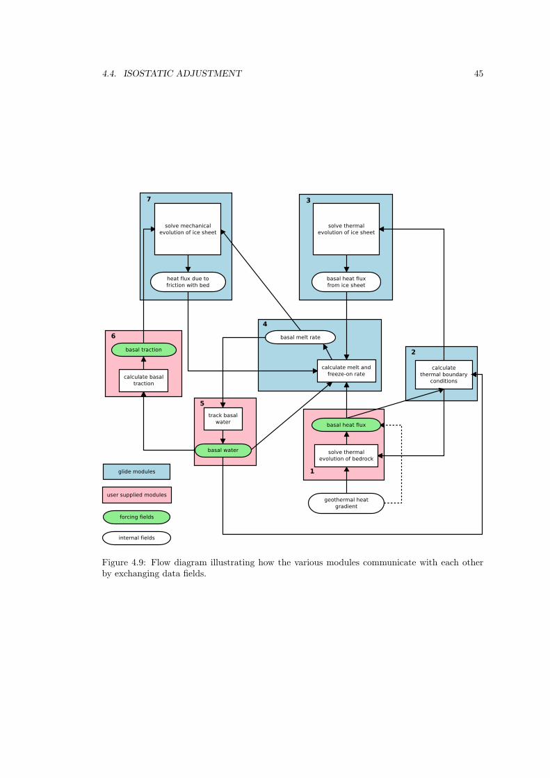
4.4. ISOSTATIC ADJUSTMENT 45
Figure 4.9: Flow diagram illustrating how the various modules communicate with each otherby exchanging data fields.
46 CHAPTER 4. SHALLOW ICE DYNAMICS: GLIDE DYNAMICAL CORE
elastic lithosphere: the flexural rigidity is taken into account;
while the mantle is treated as a
fluid mantle: the mantle behaves like a non-viscous fluid, with isostatic equilibrium reachedinstantaneously; or
relaxing mantle: the flow within the mantle is approximated by an exponentially decayinghydrostatic response function, i.e. the mantle is treated as a viscous half space.
4.4.1 Calculation of ice-water load
At each isostasy time step, the load of ice and water is calculated as an equivalent mantle-depth(L). If the basal elevation is above sea level, the load is simply due to the ice:
L =ρiρm
H, (4.75)
whereH is the ice thickness, with ρi and ρm being the densities of the ice and mantle respectively.In the case where the bedrock is below sea level, the load is calculated is that due to a changein sea level and/or the presence of non-floating ice. When the ice is floating (ρiH < ρo(z0−h)),the load is due only to sea-level changes:
L =ρoρm
z0, (4.76)
whereas when the ice is grounded, it displaces the water and adds an additional load:
L =ρiH + ρobr
ρm. (4.77)
Here, ρo is the density of sea water, z0 is the change in sea-level relative to a reference level, andbr is the bedrock elevation relative to the same reference level. The value of br will be negativefor submerged bedrock, hence the plus sign in (4.77).
4.4.2 Elastic lithosphere model
The elastic model is selected by setting lithosphere = 1 in the configuration file. By simulat-ing the deformation of the lithosphere, the deformation seen by the asthenosphere beneath iscalculated. In the absence of this model, the deformation is that due to Archimedes’ Principle,as though the load were floating on the asthenosphere.
The elastic lithosphere model is based on work by Lambeck and Nakiboglu (1980), andits implementation is fully described in Hagdorn (2003). The lithosphere model affects onlythe geometry of the deformation; the timescale for isostatic adjustment is controlled by theasthenosphere model.
The load due to a single (rectangular) grid point is approximated as being applied to a discof the same area. The deformation due to a disc of ice of radius A and thickness H is given bythe following expressions. For r < A:
w(r) =ρiH
ρm
[1 + C1 Ber
(r
Lr
)+ C2 Bei
(r
Lr
)], (4.78)
and for r ≥ A:
w(r) =ρiH
ρm
[D1 Ber
(r
Lr
)+D2 Bei
(r
Lr
)+D3 Ker
(r
Lr
)+D4 Kei
(r
Lr
)], (4.79)
4.5. TIME STEP ORDERING 47
where Ber(x), Bei(x), Ker(x) and Kei(x) are Kelvin functions of zero order, Lr = (D/ρmg))1/4
is the radius of relative stiffness, and D is the flexural rigidity. The constants Ci and Di aregiven by
C1 = aKer′(a),C2 = −aKer′(a),D1 = 0,D2 = 0,D3 = aBer′(a),D4 = −aBer′(a).
(4.80)
Here, the prime indicates the first spatial derivative of the Kelvin functions.
4.4.3 Relaxing asthenosphere model
If a fluid mantle is selected, it adjusts instantly to changes in lithospheric loading. However, arelaxing mantle is also available.
4.5 Time Step Ordering
Relative to Glimmer-CISM1.x, the order of operations on each time step has been somewhatreorganized in CISM2.x. This was done for consistency with the ordering of operations usedin Glissade and to eliminate discrepancies between time levels applied in the model and thetime levels written in output files. These changes have only a minor impact on modelresults, but do result in output that will not be an exact match between the twomodel versions for the same configuration and initial conditions.
While unlikely to be of much interest to the average user, particularly if you are not migratingfrom Glimmer-CISM1.x, the details of these changes follow. Specifically, in Glimmer-CISM1.x,for a given time step, H is advanced in time relative to T and v, and, because a complete solveoccurs even at the initial time, the output for the initial time is different than the input for theprognostic variables H and T , even though no time step has occurred at that point.
In Glimmer-CISM1.x, the time-stepping loop is organized as follows:
glide_initialise(): init T, H, v
do while (t < tend)
glide_tstep_p1(): solve T
glide_tstep_p2(): solve v, H
glide_tstep_p3(): calculate some diagnostic variables, write output for time t
advance time
end do
This results in the following relation between the state of model variables and the time level atwhich they are output:
Output time: 0 1 2T 1 2 3H 1 2 3v 0 1 2
In CISM2.x, the time-stepping loop is now organized as follows:
initialize modules
initial diagnostic solve of v (and any other diagnostic variables like upper surface)
write output for time 0
do while (t <= tend)
advance time
48 CHAPTER 4. SHALLOW ICE DYNAMICS: GLIDE DYNAMICAL CORE
solve column physics: T = f(H,T)
solve prognostic variables: advection of H=f(H,v), T=f(H,v)
solve diagnostic variables: v=f(H,T)
write output for time t
end do
This results in the following relation between the state of model variables and the time level atwhich they are output:
Output time: 0 1 2T 0 1 2H 0 1 2v 0 1 2
Chapter 5
Introduction to Higher-Order IceDynamics
5.1 Higher-Order Dynamics in CISM
5.1.1 Basics
The main distinction between so-called higher-order models and 0-order (or “shallow ice”)models is that higher-order models attempt a closer approximation to solving the nonlinearStokes equations. This usually means incorporating some approximation of horizontal-stressgradients (along-flow stretching or compression and across-flow shearing) in addition to thevertical stress gradients that are accounted for in shallow ice models (Figure 5.1). This isimportant for several reasons:
• For the ice-sheet regions of greatest interest – e.g. ice streams, ice shelves, and otherregions of fast flow – horizontal-stress gradients are at least as important as vertical stressgradients. To model the flow accurately in these regions, higher-order models are required.
• The shallow-ice approximation, applied to situations in which there is basal sliding, givesrise to a singularity in the vertical velocity. Models compute the vertical velocity byintegrating the incompressibility equation:
∂w
∂z= −∂u
∂x− ∂v
∂y. (5.1)
If there is a jump from no sliding in one grid cell to sliding in an adjacent cell, the horizontalvelocity gradients at the bed will depend on the grid spacing; the horizontal gradients (andthrough incompressibility, the vertical velocity gradient and thus the vertical velocity) willbecome increasingly large as the grid spacing decreases. Obviously, this should be avoided.
• Near the grounding line (the boundary between grounded and floating ice), horizon-tal rather than vertical stresses often control the flow. Incomplete knowledge of thestresses makes it unlikely that shallow ice models will ever be able to accurately sim-ulate grounding-line advance and retreat.
• In some regions of very slow flow, like ice divides, horizontal-stress gradients are importantor dominant. Ice cores are often recovered at ice divides, and flow modeling is importantfor interpreting ice core records and using information (such as layer thickness) to inferthe past flow history in the region. In order to model that flow correctly, one must includehorizontal stresses. (At an ice divide the surface slope is ∼0, in which case vertical stress
49
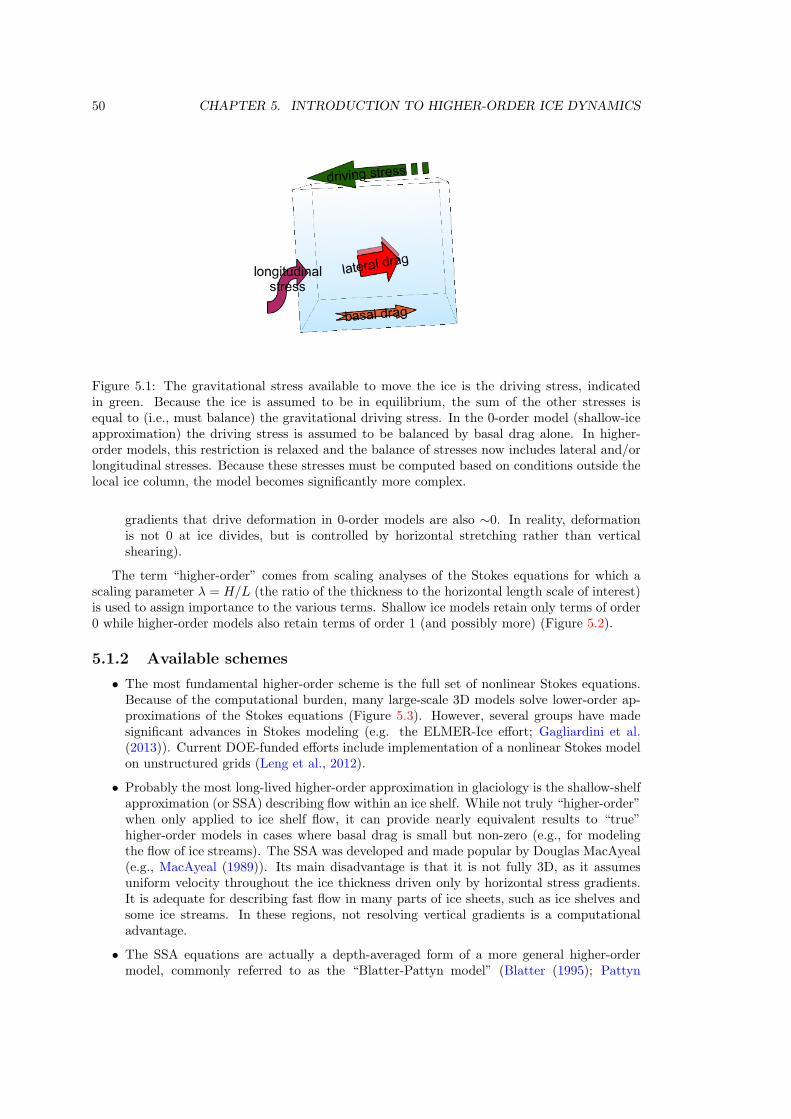
50 CHAPTER 5. INTRODUCTION TO HIGHER-ORDER ICE DYNAMICS
Figure 5.1: The gravitational stress available to move the ice is the driving stress, indicatedin green. Because the ice is assumed to be in equilibrium, the sum of the other stresses isequal to (i.e., must balance) the gravitational driving stress. In the 0-order model (shallow-iceapproximation) the driving stress is assumed to be balanced by basal drag alone. In higher-order models, this restriction is relaxed and the balance of stresses now includes lateral and/orlongitudinal stresses. Because these stresses must be computed based on conditions outside thelocal ice column, the model becomes significantly more complex.
gradients that drive deformation in 0-order models are also ∼0. In reality, deformationis not 0 at ice divides, but is controlled by horizontal stretching rather than verticalshearing).
The term “higher-order” comes from scaling analyses of the Stokes equations for which ascaling parameter λ = H/L (the ratio of the thickness to the horizontal length scale of interest)is used to assign importance to the various terms. Shallow ice models retain only terms of order0 while higher-order models also retain terms of order 1 (and possibly more) (Figure 5.2).
5.1.2 Available schemes
• The most fundamental higher-order scheme is the full set of nonlinear Stokes equations.Because of the computational burden, many large-scale 3D models solve lower-order ap-proximations of the Stokes equations (Figure 5.3). However, several groups have madesignificant advances in Stokes modeling (e.g. the ELMER-Ice effort; Gagliardini et al.(2013)). Current DOE-funded efforts include implementation of a nonlinear Stokes modelon unstructured grids (Leng et al., 2012).
• Probably the most long-lived higher-order approximation in glaciology is the shallow-shelfapproximation (or SSA) describing flow within an ice shelf. While not truly “higher-order”when only applied to ice shelf flow, it can provide nearly equivalent results to “true”higher-order models in cases where basal drag is small but non-zero (e.g., for modelingthe flow of ice streams). The SSA was developed and made popular by Douglas MacAyeal(e.g., MacAyeal (1989)). Its main disadvantage is that it is not fully 3D, as it assumesuniform velocity throughout the ice thickness driven only by horizontal stress gradients.It is adequate for describing fast flow in many parts of ice sheets, such as ice shelves andsome ice streams. In these regions, not resolving vertical gradients is a computationaladvantage.
• The SSA equations are actually a depth-averaged form of a more general higher-ordermodel, commonly referred to as the “Blatter-Pattyn model” (Blatter (1995); Pattyn
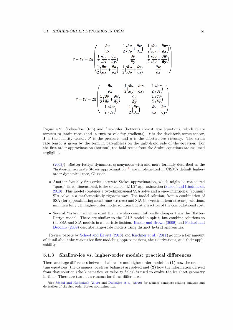
5.1. HIGHER-ORDER DYNAMICS IN CISM 51
Figure 5.2: Stokes-flow (top) and first-order (bottom) constitutive equations, which relatestresses to strain rates (and in turn to velocity gradients). τ is the deviatoric stress tensor,I is the identity tensor, P is the pressure, and η is the effective ice viscosity. The strainrate tensor is given by the term in parentheses on the right-hand side of the equation. Forthe first-order approximation (bottom), the bold terms from the Stokes equations are assumednegligible.
(2003)). Blatter-Pattyn dynamics, synonymous with and more formally described as the“first-order accurate Stokes approximation”1, are implemented in CISM’s default higher-order dynamical core, Glissade.
• Another formally first-order accurate Stokes approximation, which might be considered“quasi” three-dimensional, is the so-called “L1L2” approximation (Schoof and Hindmarsh,2010). This model combines a two-dimensional SSA solve and a one-dimensional (column)SIA solve in a mathematically rigorous way. The model solution, from a combination ofSSA (for approximating membrane stresses) and SIA (for vertical shear stresses) solutions,mimics a fully 3D, higher-order model solution but at a fraction of the computational cost.
• Several “hybrid” schemes exist that are also computationally cheaper than the Blatter-Pattyn model. These are similar to the L1L2 model in spirit, but combine solutions tothe SSA and SIA models in a heuristic fashion. Bueler and Brown (2009) and Pollard andDeconto (2009) describe large-scale models using distinct hybrid approaches.
Review papers by Schoof and Hewitt (2013) and Kirchner et al. (2011) go into a fair amountof detail about the various ice flow modeling approximations, their derivations, and their appli-cability.
5.1.3 Shallow-ice vs. higher-order models: practical differences
There are large differences between shallow-ice and higher-order models in (1) how the momen-tum equations (the dynamics, or stress balance) are solved and (2) how the information derivedfrom that solution (the kinematics, or velocity fields) is used to evolve the ice sheet geometryin time. There are two main reasons for these differences:
1See Schoof and Hindmarsh (2010) and Dukowicz et al. (2010) for a more complete scaling analysis andderivation of the first-order Stokes approximation.
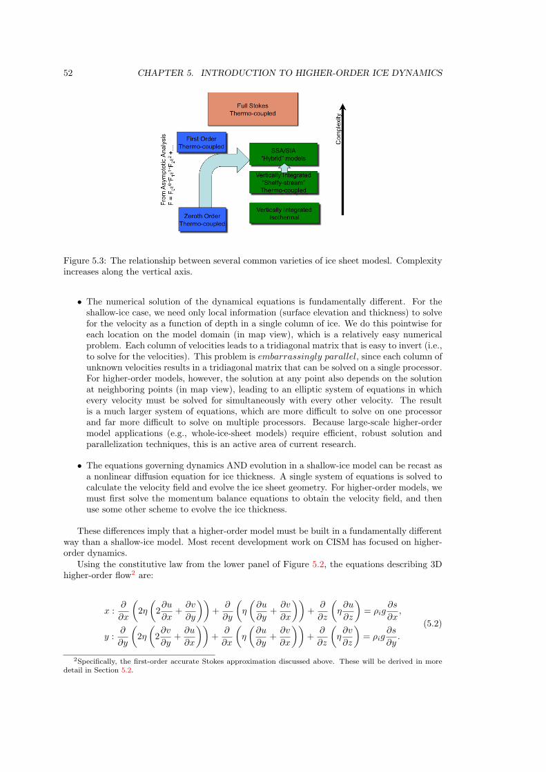
52 CHAPTER 5. INTRODUCTION TO HIGHER-ORDER ICE DYNAMICS
Figure 5.3: The relationship between several common varieties of ice sheet modesl. Complexityincreases along the vertical axis.
• The numerical solution of the dynamical equations is fundamentally different. For theshallow-ice case, we need only local information (surface elevation and thickness) to solvefor the velocity as a function of depth in a single column of ice. We do this pointwise foreach location on the model domain (in map view), which is a relatively easy numericalproblem. Each column of velocities leads to a tridiagonal matrix that is easy to invert (i.e.,to solve for the velocities). This problem is embarrassingly parallel, since each column ofunknown velocities results in a tridiagonal matrix that can be solved on a single processor.For higher-order models, however, the solution at any point also depends on the solutionat neighboring points (in map view), leading to an elliptic system of equations in whichevery velocity must be solved for simultaneously with every other velocity. The resultis a much larger system of equations, which are more difficult to solve on one processorand far more difficult to solve on multiple processors. Because large-scale higher-ordermodel applications (e.g., whole-ice-sheet models) require efficient, robust solution andparallelization techniques, this is an active area of current research.
• The equations governing dynamics AND evolution in a shallow-ice model can be recast asa nonlinear diffusion equation for ice thickness. A single system of equations is solved tocalculate the velocity field and evolve the ice sheet geometry. For higher-order models, wemust first solve the momentum balance equations to obtain the velocity field, and thenuse some other scheme to evolve the ice thickness.
These differences imply that a higher-order model must be built in a fundamentally differentway than a shallow-ice model. Most recent development work on CISM has focused on higher-order dynamics.
Using the constitutive law from the lower panel of Figure 5.2, the equations describing 3Dhigher-order flow2 are:
x :∂
∂x
(2η
(2∂u
∂x+
∂v
∂y
))+
∂
∂y
(η
(∂u
∂y+
∂v
∂x
))+
∂
∂z
(η∂u
∂z
)= ρig
∂s
∂x,
y :∂
∂y
(2η
(2∂v
∂y+
∂u
∂x
))+
∂
∂x
(η
(∂u
∂y+
∂v
∂x
))+
∂
∂z
(η∂v
∂z
)= ρig
∂s
∂y.
(5.2)
2Specifically, the first-order accurate Stokes approximation discussed above. These will be derived in moredetail in Section 5.2.
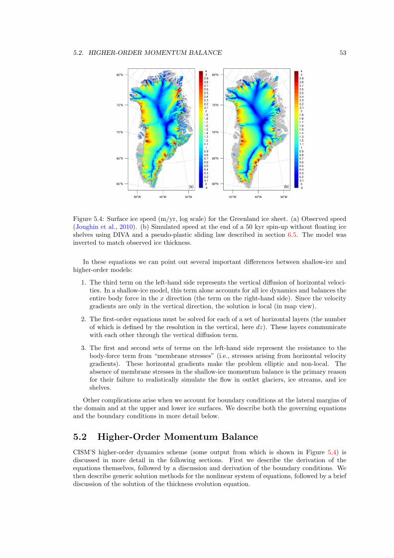
5.2. HIGHER-ORDER MOMENTUM BALANCE 53
Figure 5.4: Surface ice speed (m/yr, log scale) for the Greenland ice sheet. (a) Observed speed(Joughin et al., 2010). (b) Simulated speed at the end of a 50 kyr spin-up without floating iceshelves using DIVA and a pseudo-plastic sliding law described in section 6.5. The model wasinverted to match observed ice thickness.
In these equations we can point out several important differences between shallow-ice andhigher-order models:
1. The third term on the left-hand side represents the vertical diffusion of horizontal veloci-ties. In a shallow-ice model, this term alone accounts for all ice dynamics and balances theentire body force in the x direction (the term on the right-hand side). Since the velocitygradients are only in the vertical direction, the solution is local (in map view).
2. The first-order equations must be solved for each of a set of horizontal layers (the numberof which is defined by the resolution in the vertical, here dz). These layers communicatewith each other through the vertical diffusion term.
3. The first and second sets of terms on the left-hand side represent the resistance to thebody-force term from “membrane stresses” (i.e., stresses arising from horizontal velocitygradients). These horizontal gradients make the problem elliptic and non-local. Theabsence of membrane stresses in the shallow-ice momentum balance is the primary reasonfor their failure to realistically simulate the flow in outlet glaciers, ice streams, and iceshelves.
Other complications arise when we account for boundary conditions at the lateral margins ofthe domain and at the upper and lower ice surfaces. We describe both the governing equationsand the boundary conditions in more detail below.
5.2 Higher-Order Momentum Balance
CISM’S higher-order dynamics scheme (some output from which is shown in Figure 5.4) isdiscussed in more detail in the following sections. First we describe the derivation of theequations themselves, followed by a discussion and derivation of the boundary conditions. Wethen describe generic solution methods for the nonlinear system of equations, followed by a briefdiscussion of the solution of the thickness evolution equation.
54 CHAPTER 5. INTRODUCTION TO HIGHER-ORDER ICE DYNAMICS
The higher-order scheme is based on the 3D first-order accurate Stokes approximation (oftenreferred to as the “Blatter-Pattyn” model). The starting point is the nonlinear Stokes equations:
x :∂τxx∂x
+∂τxy∂y
+∂τxz∂z
− ∂P
∂x= 0,
y :∂τxy∂x
+∂τyy∂y
+∂τyz∂z
− ∂P
∂y= 0,
z :∂τxz∂x
+∂τzy∂y
+∂τzz∂z
− ∂P
∂z= ρig,
(5.3)
where P is the pressure and τ is the deviatoric stress tensor. The latter is given by τij =σij + Pδij , where σ is the full stress tensor.
There are a number of ways to argue that, due to the shallowness of ice sheets (i.e., thesmall value of H /L, where H is the thickness and L is a relevant horizontal length scale), theStokes equations can be reduced to the following first-order approximation:
x :∂τxx∂x
+∂τxy∂y
+∂τxz∂z
− ∂P
∂x= 0,
y :∂τyy∂y
+∂τxy∂x
+∂τyz∂z
− ∂P
∂y= 0,
z :∂τzz∂z
− ∂P
∂z= ρg.
(5.4)
The arguments supporting this reduction are fairly complex and are based on either a variationalanalysis or an asymptotic analysis (see Schoof and Hindmarsh (2010) and Dukowicz et al. (2010)for details).
The third (vertical) balance equation in (5.4) can be integrated vertically to give an expres-sion for the pressure:
P = ρg (s− z) + τzz(z). (5.5)
This is simply a statement that the full vertical normal stress is balanced by the hydrostaticpressure (the so-called hydrostatic assumption). This expression can be substituted into thehorizontal pressure gradient terms above to remove pressure from the equations. For example,for the x component of velocity we have
∂τxx∂x
+∂τxy∂y
+∂τxz∂z
=∂
∂x[ρg (s− z) + τzz(z)]
∂τxx∂x
− ∂τzz∂x
+∂τxy∂y
+∂τxz∂z
= ρg∂s
∂x
(5.6)
Using the incompressibility constraint (5.1) and the assumption that stress and strain are alignedwe can write
τzz = −τxx − τyy. (5.7)
Taking the gradient of (5.7) with respect to x, we can rewrite the vertical normal deviatoricstress in terms of horizontal normal deviatoric stresses:
− ∂τzz∂x
= − ∂
∂x(−τxx − τyy) =
∂τxx∂x
+∂τyy∂x
. (5.8)
Substituting (5.8) into (5.6), we obtain
5.2. HIGHER-ORDER MOMENTUM BALANCE 55
∂
∂x(2τxx + τyy) +
∂τxy∂y
+∂τxz∂z
= ρg∂s
∂x. (5.9)
Similarly, the y horizontal balance equation is
∂
∂y(2τyy + τxx) +
∂τxy∂x
+∂τyz∂z
= ρg∂s
∂y. (5.10)
At this point we have removed the vertical balance equation entirely; it has been incorporatedinto the horizontal balance equations through incompressibility.
Next we write these equations in terms of the velocities for which we are ultimately solving.Stresses and velocities are linked through the constitutive law for ice, which relates strain ratesto stresses (here we assume Nye’s generalization of Glen’s law), and through the definition ofthe strain rate tensor, which relates strain rates to velocity gradients:
1. τij = Bε1−nn
e εij , B = B(T )
2. εij =1
2
(∂ui
∂xj+
∂uj
∂xi
)3. 2εe = εij εij
4. η ≡ 1
2Bε
1−nn
e
5. τij = 2ηεij
(5.11)
In order, the five expressions above give:
1. Glen’s flow law3, where B = A−1n is the temperature dependent rate factor
2. The definition of the strain-rate tensor in terms of velocity gradients
3. The definition of the effective strain rate, εe, a norm of the strain-rate tensor
4. A definition of the “effective viscosity” (after rearranging some terms in (1))
5. Items (1)-(4) allow us to write the relationship between stress and strain in a standard“Newtonian” way, but with a non-Newtonian (nonlinear) viscosity.
Taking these definitions into the stress balance equations (5.9) and (5.10) and expanding interms of strain rates and effective viscosity, we have (for the x direction only):
x : 2∂
∂x(2ηεxx) +
∂
∂x(2ηεyy) +
∂
∂y(2ηεxy) +
∂
∂z(2ηεxz) = ρg
∂s
∂x, (5.12)
Replacing strain-rate components with velocity gradients, we obtain
x :∂
∂x
(4η
∂u
∂x+ 2η
∂v
∂y
)+
∂
∂y
[η
(∂u
∂y+
∂v
∂x
)]+
∂
∂z
(η∂u
∂z
)= ρg
∂s
∂x. (5.13)
An analogous expression gives the y-direction momentum balance:
y :∂
∂y
(4η
∂v
∂y+ 2η
∂u
∂x
)+
∂
∂x
[η
(∂u
∂y+
∂v
∂x
)]+
∂
∂z
(η∂v
∂z
)= ρg
∂s
∂y. (5.14)
These are the basic equations to be discretized and solved.
3Technically, we are using the inverse form of the flow-law here.
56 CHAPTER 5. INTRODUCTION TO HIGHER-ORDER ICE DYNAMICS
5.3 Higher-Order Model Boundary Conditions
We now carry out an approximate derivation of the boundary conditions in a higher-orderscheme. By “approximate” we mean that some of the derivation is guided by physical intuitionand reasonable arguments, rather than rigorous mathematics. In the end, we derive the sameset of equations as when following the more rigorous approach (e.g., Dukowicz et al. (2010)).We will consider the boundary conditions in three parts: (1) the free surface BC, (2) the basaltraction BC, and (3) lateral BCs.
5.3.1 Stress-free surface
At the upper ice surface, a stress-free boundary condition is applied. The traction vector Ti
must be continuous across the ice sheet surface and, assuming that atmospheric pressure andsurface tension are small, we have
Ti = −Ti(boundary) ≈ 0,
Ti = σijnj = σi1n1 + σi2n2 + σi3n3 = 0,(5.15)
where the ni are the components of the outward-facing, unit normal vector in Cartesian coor-dinates.
For a function F(x,y,z) = z – f(x,y) = 0, where z = f(x,y) defines the surface, the gradientof F(x,y,z) gives the components of the surface normal vector. For the case of the ice sheetsurface, s = f(x, y) and the surface normal is given by
ni =
(− ∂s
∂x,−∂s
∂y, 1
)1
a, (5.16)
where
a =
√(∂s
∂x
)2
+
(∂s
∂y
)2
+ 1. (5.17)
Eq. (5.15) gives three equations that must be satisfied at the free surface:
i = x : Tx = σxxnx + σxyny + σxznz = 0,
i = y : Ty = σyxnx + σyyny + σyznz = 0,
i = z : Tz = σzxnx + σzyny + σzznz = 0.
(5.18)
Expanding the z equation and expressing stresses in terms of strain rates and pressures, whereη is the effective viscosity defined above, gives
(2ηεzx)nx + (2ηεzy)ny + (2ηεzz − P )nz = 0. (5.19)
Solving for the pressure gives
Pnz = (2ηεzz)nz + (2ηεzx)nx + (2ηεzy)ny. (5.20)
Expanding in terms of velocity gradients and normal vector components, we find
P = 2η∂w
∂z−(η∂u
∂z
)∂s
∂x−(η∂v
∂z
)∂s
∂y, (5.21)
where we have made the usual first-order approximation that
5.3. HIGHER-ORDER MODEL BOUNDARY CONDITIONS 57
∂w
∂x=
∂w
∂y≈ 0. (5.22)
and also assumed a ≈ 1.We use this expression for the pressure and expand the two horizontal boundary condition
expressions
i = x : Tx = σxxnx + σxyny + σxznz = 0,
i = y : Ty = σyxnx + σyyny + σyznz = 0,(5.23)
in terms of velocity gradients and the effective viscosity to obtain
x : −2η∂u
∂x
∂s
∂x− η
(∂u
∂y+
∂v
∂x
)∂s
∂y+ η
∂u
∂z=
− 2η∂w
∂z
∂s
∂x+ η
∂u
∂z
[∂s
∂x
∂s
∂x
]+ η
∂v
∂z
[∂s
∂y
∂s
∂x
],
y : −2η∂v
∂y
∂s
∂y− η
(∂u
∂y+
∂v
∂x
)∂s
∂x+ η
∂v
∂z=
− 2η∂w
∂z
∂s
∂y+ η
∂u
∂z
[∂s
∂x
∂s
∂y
]+ η
∂v
∂z
[∂s
∂y
∂s
∂y
].
(5.24)
In both these expressions, the terms in square brackets are ∼ 0 (because slopes on ice sheetsare small and the slope squared is exceedingly small). From continuity, we also have
∂w
∂z= −∂u
∂x− ∂v
∂y. (5.25)
Using this expression for the normal vertical velocity gradient and removing the terms in squarebrackets, our two horizontal BC expressions become
x : −2η∂u
∂x
∂s
∂x− η
(∂u
∂y+
∂v
∂x
)∂s
∂y+ η
∂u
∂z= 2η
(∂u
∂x
∂s
∂x+
∂v
∂y
∂s
∂x
),
y : −2η∂v
∂y
∂s
∂y− η
(∂u
∂y+
∂v
∂x
)∂s
∂x+ η
∂v
∂z= 2η
(∂u
∂x
∂s
∂y+
∂v
∂y
∂s
∂y
).
(5.26)
Moving terms to one side and dividing through by the effective viscosity η, we arrive at thefinal form of the first-order, free surface boundary conditions
x : 4∂u
∂x
∂s
∂x+
∂u
∂y
∂s
∂y+ 2
∂v
∂y
∂s
∂x+
∂v
∂x
∂s
∂y− ∂u
∂z= 0,
y : 4∂v
∂y
∂s
∂y+
∂v
∂x
∂s
∂x+ 2
∂u
∂x
∂s
∂y+
∂u
∂y
∂s
∂x− ∂v
∂z= 0.
(5.27)
5.3.2 Specified basal traction
Derivation of the basal boundary condition follows that above for the free surface except that
1. The right-hand side of the equation is not zero, but rather consists of an assumed basaltraction vector with components
τbi = (τbx, τby) . (5.28)
58 CHAPTER 5. INTRODUCTION TO HIGHER-ORDER ICE DYNAMICS
2. The outward-facing normal vector components now consist of horizontal gradients in thebasal surface (with a resulting sign switch on the x, y, z components relative to the uppersurface).
3. the effective viscosity does not disappear from the equations when we divide through.
Making these substitutions, we obtain the first-order basal boundary conditions for a speci-fied basal traction:
x : 4∂u
∂x
∂b
∂x+
∂u
∂y
∂b
∂y+ 2
∂v
∂y
∂b
∂x+
∂v
∂x
∂b
∂y− ∂u
∂z=
τbxη
,
y : 4∂v
∂y
∂b
∂y+
∂v
∂x
∂b
∂x+ 2
∂u
∂x
∂b
∂y+
∂u
∂y
∂b
∂x− ∂v
∂z=
τbyη
.
(5.29)
We assume that basal traction is linearly related to basal sliding velocity through a positivetraction parameter, β, such that
τbx = −βu|z=b , τby = −βv|z=b . (5.30)
The minus sign in front of the β indicates that the traction vector is oriented parallel to and inthe opposite direction of the sliding velocity vector.
Substituting this expression into (5.29) gives the final horizontal boundary conditions at theice sheet base:
x : 4∂u
∂x
∂b
∂x+
∂u
∂y
∂b
∂y+ 2
∂v
∂y
∂b
∂x+
∂v
∂x
∂b
∂y− ∂u
∂z+
(β
η
)u = 0,
y : 4∂v
∂y
∂b
∂y+
∂v
∂x
∂b
∂x+ 2
∂u
∂x
∂b
∂y+
∂u
∂y
∂b
∂x− ∂v
∂z+
(β
η
)v = 0.
(5.31)
The use of a linear traction parameter as in (5.30) can be modified to implement basal frictionlaws that are a function of effective pressure (ice overburden pressure minus water pressure atthe bed) and generally are nonlinear in the sliding velocity. Two such basal friction laws areimplemented in CISM. For friction laws that are nonlinear in sliding velocity, β in (5.30) becomesa function of sliding velocity. This is implemented by lagging the value of sliding velocity usedto calculate an “effective” β in the fixed-point iterations used to solve the momentum balance.
The first is a Weertman-style friction law (Weertman, 1957, 1964) modified to include aneffective pressure dependence (Bindschadler, 1983; Budd et al., 1979). Notation here followsthe summary by Cuffey and Paterson (2010, p.240, eq. 7.17). The form of the friction law is:
ub = kτbpN−q, (5.32)
which can be rearranged for τb as:
τb = k−1p ub
1pN
qp , (5.33)
where k is a friction coefficient based on thermal and mechanical properties of ice and is inverselyrelated to bed roughness. Cuffey and Paterson (2010) suggest values of p = 3 and q = 1, makingthe basal friction nonlinear in velocity.
One problem with (5.32) is that it allows for unbounded basal traction. CISM also includesa physically-based basal friction law for sliding over hard beds that allows for cavitation andbounded basal drag (Schoof, 2005). In this law, the friction is related to the velocity andeffective pressure by
τb = C
(ub
ub +NnΛ
)1/n
N, Λ =λmaxA
mmax. (5.34)
5.3. HIGHER-ORDER MODEL BOUNDARY CONDITIONS 59
In Eq. 5.34, C is a Coulomb friction coefficient, and λmax and mmax are the wavelength (m)and maximum slope, respectively, of the dominant bedrock bumps. Near cavitation (i.e., wheneffective pressure approaches 0 at high water pressure), the friction law becomes a Coulombfriction law of the form τb = CN . Alternatively, at large effective pressures (i.e., low water
pressure), the friction law takes a power law form, τb ∝ u1/nb . The representation of bump
geometry in the friction law is at a sub-grid scale and is not explicitly resolved by the model.The release version of CISM does not currently include a hydrology model that computes
effective pressure, so at present the effective pressure fields must be input as data to use thesetwo basal friction laws.
5.3.3 Specified basal yield stress
The above implementation of a specified basal traction can be altered to simulate sliding overa sediment-covered bed for which the sediment has a plastic or “Coulomb friction” rheology.That is, sliding does not occur below the specified yield stress of the underlying material (e.g., awater-saturated subglacial till). When the yield stress, τ0 is reached, sliding occurs at a rate thatmaintains but does not exceed that yield stress. Consider the x–direction boundary conditionin (5.29), written out in terms of basal stress components:
x : 4η∂u
∂x
∂b
∂x+ η
∂u
∂y
∂b
∂y+ 2η
∂v
∂y
∂b
∂x+ η
∂v
∂x
∂b
∂y− η
∂u
∂z= τbx,
τbx ≈ τ0 = τ0
(u
|u|
)= τ0
(u√
u20 + v20 + γ
).
(5.35)
In this expression, u is the x component of the basal sliding velocity from the currentiteration, u0 and v0 are components from the previous iteration, and γ is a regularizationconstant (a small number to avoid division by zero during early iterations). As the solutionconverges, velocities at the current and previous iteration are nearly equal, and the expressionin parentheses approaches 1, in which case the basal stress and yield stress are approximatelyequal.
We can accommodate this plastic behavior in our earlier framework by treating β as nonlinearand dependent on the velocity:
τbx = −βu,
β ≡ τ0√u20 + v20 + γ
,
τbx = −
(τ0√
u20 + v20 + γ
)u.
(5.36)
This expression for nonlinear β can be substituted in the expression (5.31) for the basal bound-ary conditions. Figure 5.5 shows an example of this type of boundary condition for the case ofan idealized ice stream simulated by CISM.
5.3.4 Lateral boundary conditions
Currently, the only significant lateral boundary condition implemented in CISM is that forfloating ice; the depth-averaged stress resulting from an adjacent column of ocean water isapplied at the location of an ice shelf (or ice tongue) front. The derivation largely followsthose for the free surface and specified basal traction boundary conditions, except that thesurface normal vectors, nx and ny, are taken as lying entirely in the x, y plane (i.e., they areperpendicular to a vertical shelf front). Thus we have
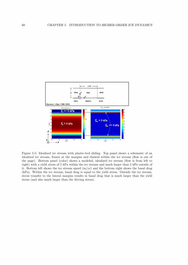
60 CHAPTER 5. INTRODUCTION TO HIGHER-ORDER ICE DYNAMICS
Figure 5.5: Idealized ice stream with plastic-bed sliding. Top panel shows a schematic of anidealized ice stream, frozen at the margins and thawed within the ice stream (flow is out ofthe page). Bottom panel (color) shows a modeled, idealized ice stream (flow is from left toright) with a yield stress of 5 kPa within the ice stream and much larger than 5 kPa outside ofit. Bottom left shows the ice stream speed (m/yr) and the bottom right shows the basal drag(kPa). Within the ice stream, basal drag is equal to the yield stress. Outside the ice stream,stress transfer to the lateral margins results in basal drag that is much larger than the yieldstress (and also much larger than the driving stress).
5.3. HIGHER-ORDER MODEL BOUNDARY CONDITIONS 61
x : 4η∂u
∂xnx + η
∂u
∂yny + η
∂u
∂znz = −2η
∂v
∂ynx − η
∂v
∂xny + ρg (s− z)nx − Sx,
y : 4η∂v
∂yny + η
∂v
∂xnx + η
∂v
∂znz = −2η
∂u
∂xny − η
∂u
∂ynx + ρg (s− z)ny − Sy.
(5.37)
Here, Sx and Sy are source terms from the pressure due to ocean water (to be defined below),and ρg (s− z) comes from including the first-order vertical stress balance:
∂σzz
∂z=
∂τzz∂z
− ∂P
∂z= ρg (integrate w.r.t. z),
P = ρg (s− z) + τzz,
P = ρg (s− z) + 2ηεzz = ρg (s− z) + 2η
(−∂u
∂x− ∂v
∂y
),
(5.38)
with ρ being the ice density. In the last step above we have used the constitutive relationand incompressibility to expand the vertical, normal-deviatoric stress in terms of the effectiveviscosity and horizontal-normal strain rates. We calculate the source terms Sx and Sy as thedepth-averaged stress at the ice shelf front due to the pressure of ocean water there. This valueis given by
Si =
[1
H
1
2ρwg (H − hf )
2
]ni =
[1
2ρwgH
(ρ
ρw
)2]ni, hf = H
(1− ρ
ρw
), (5.39)
where i=x,y, ni is the shelf-front normal vector, H is the ice thickness, hf is the “freeboard”,or ice thickness above flotation, and ρw is the density of ocean water. Because we have taken adepth average for this source term, we take a depth average of the term ρg (s− z) above, whichis 1
2ρgH.Combining these two terms and inserting them in the horizontal boundary condition expres-
sions above gives
x : 4η∂u
∂xnx + η
∂u
∂yny + η
∂u
∂znz =
− 2η∂v
∂ynx − η
∂v
∂xny +
[−1
2H
(ρ
ρw
)2
ρwg +1
2ρgH
]nx,
y : 4η∂v
∂yny + η
∂v
∂xnx + η
∂v
∂znz =
− 2η∂u
∂xny − η
∂u
∂ynx +
[−1
2H
(ρ
ρw
)2
ρwg +1
2ρgH
]ny,
(5.40)
which can be rearranged to
x : 4∂u
∂xnx +
∂u
∂yny +
∂u
∂znz + 2
∂v
∂ynx +
∂v
∂xny =
ρgH
2η
(1− ρ
ρw
)nx,
y : 4∂v
∂yny +
∂v
∂xnx +
∂v
∂znz + 2
∂u
∂xny +
∂u
∂ynx =
ρgH
2η
(1− ρ
ρw
)ny.
(5.41)
For an ice shelf, the surface and basal velocities are equal, in which case the vertical velocitygradient terms are ∼ 0, giving the final form of the lateral boundary conditions:
62 CHAPTER 5. INTRODUCTION TO HIGHER-ORDER ICE DYNAMICS
x : 4∂u
∂xnx +
∂u
∂yny + 2
∂v
∂ynx +
∂v
∂xny =
ρgH
2η
(1− ρ
ρw
)nx,
y : 4∂v
∂yny +
∂v
∂xnx + 2
∂u
∂xny +
∂u
∂ynx =
ρgH
2η
(1− ρ
ρw
)ny.
(5.42)
5.3.5 Summary
All the boundary conditions above have a similar form. In fact, all that differs among the equa-tions for the free surface, the specified basal traction, and the lateral shelf boundary conditionis (1) the definition of the normal vectors and (2) the existence and definition of a source term.Here are the x–direction equations again for the three cases:
x : 4∂u
∂x
∂s
∂x+
∂u
∂y
∂s
∂y+ 2
∂v
∂y
∂s
∂x+
∂v
∂x
∂s
∂y− ∂u
∂z= 0,
x : 4∂u
∂x
∂b
∂x+
∂u
∂y
∂b
∂y+ 2
∂v
∂y
∂b
∂x+
∂v
∂x
∂b
∂y− ∂u
∂z=
τbxη
,
x : 4∂u
∂xnx +
∂u
∂yny + 2
∂v
∂ynx +
∂v
∂xny =
ρgH
2η
(1− ρ
ρw
)nx.
(5.43)
In the first equation (free surface), the normals are related to the ice sheet surface slope and thesource term is zero (which allows us to divide through by the effective viscosity and remove itfrom the equations). In the second equation (specified basal traction), the normals are relatedto the bedrock slopes and the source term is related to the assumed relationship between thebasal shear stress and the basal sliding rate. In the last equation, the normals are defined bythe shape of the ice-shelf front in map view, the vertical velocity gradient terms are absent, andthe source term is related to the pressure from the adjacent column of ocean water.
In CISM’s earlier developmental dycore, Glam, these boundary conditions were implementedusing finite differences, leading to significant complexity. The current dycore, Glissade, solvesfor ice velocity using a finite-element approach, in which boundary conditions are handledmore simply. For example, the surface boundary condition is a “natural” BC that is satisfiedautomatically. See, e.g., Dukowicz et al. (2010) for details.
5.4 Numerical Solution of Higher-Order Equations
This section describes numerical methods for solving the higher-order equations discussed above.More specific details are given in Chapter 6.
5.4.1 Governing matrix equations
We would like to solve the stress-balance equations (5.13) and (5.14) for the horizontal velocitycomponents u and v. Any number of standard methods (e.g., finite differences, finite volumes,or finite elements) can be used to discretize these governing equations: i.e., to re-formulate themfrom their continuous, PDE form to a discontinuous, piecewise, algebraic approximation basedon a specific computational mesh. In the limit, as the mesh spacing goes to zero, the differencebetween the solution to the actual PDE and its algebraic approximation also goes to zero. TheGlissade dynamical core uses the Finite Element Method (FEM) to discretize the governingequations, as discussed in Chapter 6. The result of the discretization is a set of linear algebraicequations that can be written in matrix form. An example is given below, where the coefficientsof u and v are contained in block matrices A, given by
5.5. THICKNESS EVOLUTION IN HIGHER-ORDER MODELS 63
[Auu Auv
Avu Avv
] [uv
]=
[bu
bv
],
Auuu+Auvv = bu, Avuu+Avvv = bv.
(5.44)
Here the uu subscript denotes block matrices containing coefficients for gradients of u in theequation for the x component of velocity (i.e., u). The subscript uv denotes block matricescontaining coefficients for gradients of v in the equation for the x component of velocity (andsimilarly for the vu and vv subscripts). On the right-hand side, the subscripts u and v areattached to the geometric source terms for the x and y components of velocity, respectively.
5.4.2 Treating nonlinearity through a fixed-point iteration
The nonlinearity of the equations—the fact that the matrix coefficients (in particular, the effec-tive viscosity) depend on the velocity (or more specifically, the velocity gradients)—is handledthrough a fixed-point iteration. A general fixed-point iteration for a vector of unknowns u canbe written as
uk = B(uk−1
), (5.45)
where k is the current iteration index and B is a matrix operation performed on the componentsof u obtained at the previous iteration, k − 1. The fixed point occurs when the values of u atk and k − 1 are equal to within some given tolerance, at which point the iteration process ishalted. For a Picard iteration, which is used in Glissade, the matrix coefficients with a velocitydependence are simply based on the velocities from the previous iteration. In other words,velocities obtained during iteration k− 1 are used to calculate the strain rates appearing in theexpression for effective viscosity at iteration k.
Accounting for the Picard iteration on the effective viscosity, the final form of the matrixequations solved by Glissade becomes
[Ak−1
uu Ak−1uv
Ak−1vu Ak−1
vv
] [uk
vk
]=
[bku
bkv
],
Ak−1uu uk +Ak−1
uv vk = bku, Ak−1
vu uk +Ak−1vv vk = bk
v,
These equations form a linear system; for the solution at any particular iteration k, the matrixcoefficients that depend on the velocity components u and v are held frozen during the solution.This linear system can be solved using a variety of methods. For large, sparse systems, thepreconditioned conjugate gradient (PCG) method or some related method (e.g., preconditionedBiCG or GMRES) is generally the most efficient. (Glissade forms a symmetric positive-definitematrix, as required for the PCG method. Auu and Avv are symmetric, and Auv = AT
vu.) Inthis case the linear system is solved not exactly, but to within some small tolerance of the truesolution.
5.5 Thickness Evolution in Higher-Order Models
5.5.1 Conservation of mass
As mentioned previously, conservation of mass for an ice sheet can be expressed by
∂H
∂t= −∇ · (UH) +B, (5.46)
64 CHAPTER 5. INTRODUCTION TO HIGHER-ORDER ICE DYNAMICS
where U = (U, V ) is the 2D, depth-integrated velocity vector, H is the ice thickness, UH isthe 2D ice flux vector, and B is the sum of surface and basal mass balance terms. The changein thickness per unit time is given by the negative of the flux divergence plus a source term.The minus sign in front of the divergence (terms in parentheses on the right-hand side) ensuressensible behavior: consider a section of the ice sheet where the thickness is nearly uniform andthere is no accumulation or ablation. If the velocity gradient along the flow is negative (the iceis slowing down), then we expect local thickening (left-hand side of the equation is > 0), and ifthe ice is speeding up along flow, we expect local thinning. This is the equation that needs tobe solved to calculate the evolution of the ice sheet geometry.
5.5.2 A diffusive approach
For the case of a shallow-ice model, U and V are expressed in terms of ice thickness and elevationgradients, in which case the problem can be recast as a diffusion equation in ice thickness. In1D, (5.46) becomes
∂H
∂t=
∂
∂x
(D
∂s
∂x
)+B, D =
2A
n+ 2(ρg)
nHn+2
∣∣∣∣ ∂s∂x∣∣∣∣n−1
, (5.47)
where the diffusivity D is nonlinear (because it depends on the solution H), A is the rate factorin Glen’s flow law, n is the power-law exponent, s is the ice surface elevation, and ρ and g arethe ice density and the acceleration due to gravity. Importantly, we need only local informationin order to solve the above equation. If the velocity cannot be solved locally, as in the case ofhigher-order models, we cannot easily use the above formulation to solve ice sheet evolution. Inan attempt to use this form and retain a diffusion-solution approach to the problem (diffusionproblems generally have favorable numerical properties), we could try the following approach(again, in 1D):
∂H
∂t=
∂
∂x
(D
∂s
∂x
)+B, D = UH
(∂s
∂x
)−1
, (5.48)
where the U in the expression for D is the depth-integrated velocity field from the higher-ordermodel. This is the approach initially taken by Pattyn (2003) in one of the first higher-ordermodeling studies to deal with this particular problem. Notice that ice sheet surface slope is inthe denominator of the diffusivity. As slopes become smaller (as they tend to do in fast-flowingice streams and ice shelves), the diffusivity grows larger, approaching infinity as the slope goesto zero. The faster velocities in these regions appear in the numerator of the diffusivity, alsomaking it larger. This is a severe restriction because, for explicit schemes, the diffusive CFLcondition requires that
∆t <(∆x)
2
2D, (5.49)
where ∆t is the time step required for numerical stability and ∆x is the grid spacing. As thediffusivity goes to infinity (i.e., for faster flows and shallower slopes), the stable time step goesto zero. Thus in practice, this approach has proven very difficult to use for calculating ice sheetevolution in the dynamically interesting areas of ice sheets. An alternate approach is needed.
5.5.3 Advection schemes
An alternate approach is to solve the evolution equation using an advection scheme. Numeri-cally, advection schemes can be more problematic than diffusion schemes, but in cases like thisone, they are difficult to avoid. One of the simplest advection schemes is a first-order, upwind-advection scheme (as above, “first-order” here refers to first-order accurate), and we will outlinethe implementation of such a scheme below.
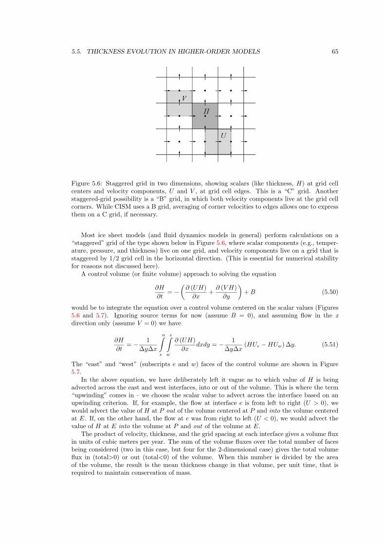
5.5. THICKNESS EVOLUTION IN HIGHER-ORDER MODELS 65
Figure 5.6: Staggered grid in two dimensions, showing scalars (like thickness, H) at grid cellcenters and velocity components, U and V , at grid cell edges. This is a “C” grid. Anotherstaggered-grid possibility is a “B” grid, in which both velocity components live at the grid cellcorners. While CISM uses a B grid, averaging of corner velocities to edges allows one to expressthem on a C grid, if necessary.
Most ice sheet models (and fluid dynamics models in general) perform calculations on a“staggered” grid of the type shown below in Figure 5.6, where scalar components (e.g., temper-ature, pressure, and thickness) live on one grid, and velocity components live on a grid that isstaggered by 1/2 grid cell in the horizontal direction. (This is essential for numerical stabilityfor reasons not discussed here).
A control volume (or finite volume) approach to solving the equation
∂H
∂t= −
(∂ (UH)
∂x+
∂ (V H)
∂y
)+B (5.50)
would be to integrate the equation over a control volume centered on the scalar values (Figures5.6 and 5.7). Ignoring source terms for now (assume B = 0), and assuming flow in the xdirection only (assume V = 0) we have
∂H
∂t= − 1
∆y∆x
n∫s
e∫w
∂ (UH)
∂xdxdy = − 1
∆y∆x(HUe −HUw)∆y. (5.51)
The “east” and “west” (subscripts e and w) faces of the control volume are shown in Figure5.7.
In the above equation, we have deliberately left it vague as to which value of H is beingadvected across the east and west interfaces, into or out of the volume. This is where the term“upwinding” comes in – we choose the scalar value to advect across the interface based on anupwinding criterion. If, for example, the flow at interface e is from left to right (U > 0), wewould advect the value of H at P out of the volume centered at P and into the volume centeredat E. If, on the other hand, the flow at e was from right to left (U < 0), we would advect thevalue of H at E into the volume at P and out of the volume at E.
The product of velocity, thickness, and the grid spacing at each interface gives a volume fluxin units of cubic meters per year. The sum of the volume fluxes over the total number of facesbeing considered (two in this case, but four for the 2-dimensional case) gives the total volumeflux in (total>0) or out (total<0) of the volume. When this number is divided by the areaof the volume, the result is the mean thickness change in that volume, per unit time, that isrequired to maintain conservation of mass.
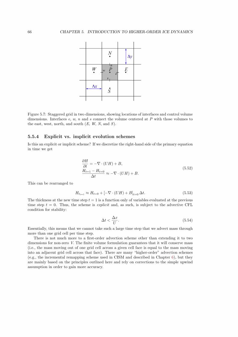
66 CHAPTER 5. INTRODUCTION TO HIGHER-ORDER ICE DYNAMICS
Figure 5.7: Staggered grid in two dimensions, showing locations of interfaces and control volumedimensions. Interfaces e, w, n and s connect the volume centered at P with those volumes tothe east, west, north, and south (E, W, N, and S ).
5.5.4 Explicit vs. implicit evolution schemes
Is this an explicit or implicit scheme? If we discretize the right-hand side of the primary equationin time we get
∂H
∂t= −∇ · (UH) +B,
Ht=1 −Ht=0
∆t≈ −∇ · (UH) +B.
(5.52)
This can be rearranged to
Htt=1≈ Ht=0 + [−∇ · (UH) +B]t=0 ∆t. (5.53)
The thickness at the new time step t = 1 is a function only of variables evaluated at the previoustime step t = 0. Thus, the scheme is explicit and, as such, is subject to the advective CFLcondition for stability:
∆t <∆x
U. (5.54)
Essentially, this means that we cannot take such a large time step that we advect mass throughmore than one grid cell per time step.
There is not much more to a first-order advection scheme other than extending it to twodimensions for non-zero V. The finite volume formulation guarantees that it will conserve mass(i.e., the mass moving out of one grid cell across a given cell face is equal to the mass movinginto an adjacent grid cell across that face). There are many “higher-order” advection schemes(e.g., the incremental remapping scheme used in CISM and described in Chapter 6), but theyare mainly based on the principles outlined here and rely on corrections to the simple upwindassumption in order to gain more accuracy.
Chapter 6
Higher-Order Ice Dynamics:Glissade Dynamical Core
6.1 Introduction
CISM includes a parallel, higher-order dynamical core called Glissade1, the successor to theGlide shallow-ice dycore. Like Glide, Glissade solves equations for conservation of momen-tum (i.e., an appropriate approximation of Stokes flow), mass, and internal energy. Glissadenumerics, however, differ substantially from Glide numerics:
• Velocity: Glide is limited to the shallow-ice approximation, whereas Glissade can solveseveral Stokes approximations, as described in Section 6.2. These include a 3D first-orderBlatter-Pattyn solver (the most accurate and complex scheme) as well as simpler solvers forthe shallow-ice approximation (SIA), shallow-shelf approximation (SSA), and a verticallyintegrated higher-order approximation. Unlike Glide, which computes the velocity usingfinite-difference techniques, Glissade uses a more robust and flexible finite-element method.
• Temperature: To evolve the ice temperature, Glide solves a prognostic equation that in-corporates horizontal advection as well as vertical heat diffusion and internal dissipation.In Glissade, temperature advection is handled by the transport scheme, and a separatemodule solves for vertical diffusion and internal dissipation. The vertical solver, describedin Section 6.3, is local; each ice column calculation is independent of other column calcu-lations.
• Mass and tracer transport: Glide solves a diffusion equation for tranport of mass (i.e.,ice thickness); this equation incorporates the local shallow-ice velocities. Since Glissadesolves for higher-order flow that may have a large advective (as oppposed to diffusive)component, a different approach is needed. Glissade has two mass- and energy-conservingtransport options, described in Section 6.4: incremental remapping (the more complexand accurate scheme) and first-order upwind. These schemes transport mass and internalenergy in the horizontal direction, followed by a vertical remapping to sigma coordinates.
Glissade numerics are described in detail below.
1The name “Glissade” was originally an acronym, but as with “Glimmer” and “Glide” the acronym is rarelyused. It can be pronounced either American–style (gliss–AID) or French–style (gliss–AHD).
67
68 CHAPTER 6. HIGHER-ORDER ICE DYNAMICS: GLISSADE DYNAMICAL CORE
6.2 Velocity Solver
Glissade computes the ice velocity by solving an appropriate approximation of the Stokes equa-tions, given the 2D surface elevation and thickness fields, the 3D temperature field, and relevantboundary conditions. The directory libglissade contains the primary higher-order velocitymodule, glissade velo higher.F90, along with supporting modules for the various solver op-tions. Section 6.2.1 describes assembly and solution of the matrix problem for the 3D first-orderBlatter-Pattyn approximation. The following sections discuss simpler approximations, includ-ing the SIA, SSA, and a depth-integrated-viscosity approximation (DIVA, based on Goldberg(2011)).
6.2.1 Blatter-Pattyn approximation
The basic equations of the Blatter-Pattyn approximation in Cartesian coordinates, repeatedfrom Section 5.2, are
x :∂
∂x
(2η
(2∂u
∂x+
∂v
∂y
))+
∂
∂y
(η
(∂u
∂y+
∂v
∂x
))+
∂
∂z
(η∂u
∂z
)= ρg
∂s
∂x,
y :∂
∂y
(2η
(2∂v
∂y+
∂u
∂x
))+
∂
∂x
(η
(∂u
∂y+
∂v
∂x
))+
∂
∂z
(η∂v
∂z
)= ρg
∂s
∂y,
(6.1)
where u and v are the components of horizontal velocity, η is the effective viscosity, s is the icesurface elevation, ρ is the density of ice (assumed constant), and g is gravitational acceleration.
As in Glide, the equations are discretized on a structured 3D mesh. In the map plane themesh consists of rectangular cells. These cells form an unstaggered 2D grid of dimension (nx, ny)(thus the number of cells is the product (nx)(ny)), together with a staggered grid of dimension(nx− 1, ny − 1). The corners of each cell (where four rectangles meet) are called vertices. Thevertical levels of the mesh are based on a terrain-following sigma coordinate system. We defineσ = (s − z)/H, where H is the ice thickness, with σ = 0 at the top surface and σ = 1 at thebed. There are nz levels in the vertical direction, with nz − 1 layers between these levels. Anelement is the region associated with a particular cell and layer; there are (nx)(ny)(nz − 1)elements on the mesh. A node is a point where eight elements intersect (or where four elementsintersect at the upper or lower surface). There are (nx− 1)(ny − 1)(nz) nodes on the mesh.
Scalar 2D fields such as H and s are defined for each cell. Scalar 3D fields such as icetemperature T lie at the center of each element (i.e., at the midpoint of each layer associatedwith each cell). Gradients of 2D scalar fields (e.g., the surface slope ∇s) are defined at vertices.The velocity components u and v live at nodes.
For problems solved in parallel, the domain is partitioned among multiple processors. Letnxlocal and nylocal be the number of locally owned cells on each processor. Each processor holdsdata for two rows of halo cells (i.e., cells belonging to other processors) surrounding the block oflocally owned cells. Thus the 2D grid on a given processor has dimensions (nxlocal+2, nylocal+2).Each locally owned cell is associated with a locally owned vertex lying at the northeast (upperright) corner of the cell.
An active cell is a cell that borders a locally owned vertex, whose ice thickness exceeds aminimum threshold. Each active cell is associated with a column of nz−1 active elements. (Allthe data in a given column resides on a single processor.) An active vertex is any vertex of anactive cell. Each active vertex is associated with nz active nodes, including nodes at the surfaceand bed.
The effective viscosity is defined in each active element by
η ≡ 1
2A
−1n ε
1−nn
e , (6.2)
6.2. VELOCITY SOLVER 69
where A is the temperature-dependent rate factor in Glen’s flow law, and εe is the effectivestrain rate, given in the Blatter-Pattyn approximation by
ε2e = ε2xx + ε2yy + εxxεyy + ε2xy + ε2xz + ε2yz, (6.3)
where
εij =1
2
(∂ui
∂xj+
∂uj
∂xi
). (6.4)
for the horizontal terms (εxx, εxy and εyy), but the vertical terms are simplified as εxz = 12∂x∂z
and εyz = 12∂y∂z . To compute the rate factor A, we assume an Arrhenius relationship:
A(T ∗) = ae−Q/RT∗, (6.5)
where T ∗ is the absolute temperature corrected for the dependence of the melting point onpressure (T ∗ = T + 8.7 · 10−4(s − z), T in Kelvin), a is a temperature–independent materialconstant (given by Paterson and Budd (1982)), Q is the activation energy for creep, and R isthe universal gas constant.
Given T , s, H, and an initial guess for u and v, the problem is to solve Eq. (6.1) for u andv at each active node. (At inactive nodes we set u = v = 0.) This problem can be written inthe form
Ax = b, (6.6)
or more fully, [Auu Auv
Avu Avv
] [uv
]=
[bu
bv
].
(6.7)
Eq. (6.7) shows the four parts of the global matrix A, with the solution and right-hand-sidevectors separated into u and v components. In Glissade, A is always symmetric and positive-definite.
Since A depends (through η) on u and v, the problem is nonlinear and must be solvediteratively (see Section 5.4.2). For each nonlinear iteration, Glissade computes the 3D η fieldbased on the current guess for the velocity field and solves a linear problem of the form (6.7).Then η is updated and the process is repeated until the solution converges to within a giventolerance. This procedure is known as Picard iteration.
The following sections describe how the matrix equations are assembled and solved.
Assembly
The coupled PDEs (6.1) are discretized using the finite-element method. Here we give a detailedbut non-rigorous description of the method as applied to the Blatter-Pattyn approximation onthe CISM mesh. We refer the reader to standard texts (e.g., Hughes, 2000; Huebner et al.,2001) for a full discussion of finite elements.
The PDEs, with appropriate boundary conditions, are converted to a system of algebraicequations by dividing the full domain into subdomains (i.e., elements), representing the velocitysolution on each element, and integrating over elements. On the CISM mesh, the elements arehexahedra (rectangles in map view), each of which has eight nodes shared with its neighbors.The solution is approximated as a sum over basis functions φ. Each active node is associatedwith a basis function whose value is φ = 1 at that node, with φ = 0 at all other nodes. Thesolution at a point within an element can be expanded in terms of basis functions and nodalvalues:
70 CHAPTER 6. HIGHER-ORDER ICE DYNAMICS: GLISSADE DYNAMICAL CORE
u(x, y, z) =∑n
φn(x, y, z)un, v(x, y, z) =∑n
φn(x, y, z)vn, (6.8)
where the sum is over the nodes of the element; un and vn are nodal values of the solution; andφn varies smoothly between 0 and 1 within the element. The fact that φ = 0 except in a smallregion ensures that the sum includes only as many terms as there are nodes per element.
Glissade uses standard finite-element techniques to represent the PDE on each element andassemble the element equations into a global set of algebraic equations of the form (6.7). Thescheme is formally equivalent to that described by Perego et al. (2012) (henceforth PGB). Eq.(6.1) can be written as
−∇ · (2ηε1) = −ρg∂s
∂x,
−∇ · (2ηε2) = −ρg∂s
∂y,
(6.9)
where
ε1 =
2εxx + εyyεxyεxz
, ε2 =
εxyεxx + 2εyy
εyz
. (6.10)
(These are Eqs. 12 and 13 in PGB.) We rewrite the equations in weak form (see PGB Eq. 15),which is obtained by multiplying (6.9) by the basis functions and integrating over the domain,using integration by parts to eliminate the second derivative:
x :
∫Ω
2ηε1(u, v) · ∇φ1 dΩ +
∫ΓB
βuφ1 dΓ +
∫ΓL
pn1φ1 dΓ +
∫Ω
ρg∂s
∂xφ1 dΩ = 0,
y :
∫Ω
2ηε2(u, v) · ∇φ2 dΩ +
∫ΓB
βuφ2 dΓ +
∫ΓL
pn2φ2 dΓ +
∫Ω
ρg∂s
∂yφ2 dΩ = 0,
(6.11)
where Ω represents the domain volume, ΓB denotes the lower boundary, ΓL denotes the lateralboundary (e.g., the calving front of an ice shelf), β is a basal traction parameter, p is the pressureat the lateral boundary, and n1 and n2 are components of the normal to ΓL. These equationscan also be obtained from a variational principle as described by Dukowicz et al. (2010).
The four terms on the LHS of (6.11) describe internal ice stresses, basal friction, lateralpressure, and the gravitational driving force, respectively. Next we describe how these termsare summed over elements and assembled into the global matrix A and right-hand side vectorb.
Internal ice stresses. We start with the internal stress term, which is the most complex.We rewrite the first term on the LHS of (6.11) in terms of velocity components:
x :
∫Ω
2η[2∂u∂x + ∂v
∂y12
(∂u∂y + ∂v
∂x
)12∂u∂z
]∂φ∂x
∂φ∂y
∂φ∂z
,
y :
∫Ω
2η[12
(∂u∂y + ∂v
∂x
)2∂v∂y + ∂u
∂x12∂v∂z
]∂φ∂x
∂φ∂y
∂φ∂z
,
(6.12)
6.2. VELOCITY SOLVER 71
where brackets are used for row vectors and braces for column vectors. Glissade evaluates (6.12)for each active element. Recall that hexahedral elements have eight nodes, with u and v to bedetermined at each active node. Inserting the velocity expressions (6.8) in (6.12), we obtain
x :
∫Ω
2η
(∂φi
∂x
(2
[∂φj
∂x
]uj+
[∂φj
∂y
]vj
)+
∂φi
∂y
(1
2
[∂φj
∂y
]uj+
1
2
[∂φj
∂x
]vj
)+
∂φi
∂z
(1
2
[∂φj
∂z
]uj
)),
y :
∫Ω
2η
(∂φi
∂y
(2
[∂φj
∂y
]vj+
[∂φj
∂x
]uj
)+
∂φi
∂x
(1
2
[∂φj
∂x
]vj+
1
2
[∂φj
∂y
]uj
)+
∂φi
∂z
(1
2
[∂φj
∂z
]vj
)).
(6.13)
Each row or column vector has eight terms, one for each node of the element. These termscan be evaluated to form a set of four 8x8 element matrices. Each row of an element matrix isassociated with u or v at a given node. The columns in this row contain terms linking the nodeto u or v at the other nodes of the same element (with the diagonal term linking the node toitself).
In the x component of (6.13), the terms that multiply uj are given by∫Ω
η
(4∂φi
∂x
∂φj
∂x+
∂φi
∂y
∂φj
∂y+
∂φi
∂z
∂φj
∂z
)dΩ. (6.14)
Letting i and j range from 1 to 8, (6.14) gives the 64 terms of the 8x8 element matrix Kuu,which links the u value at each node to the u values at all eight nodes. Similarly, the 64 termsof element matrix Kuv, which links u at each node to v at each of the eight nodes, are given by∫
Ω
η
(2∂φi
∂x
∂φj
∂y+
∂φi
∂y
∂φj
∂x
)dΩ. (6.15)
Likewise, two 8x8 matrices are associated with the y component of (6.13). The terms ofKvu, which connects v at each node to u at each of eight nodes, are given by∫
Ω
η
(2∂φi
∂y
∂φj
∂x+
∂φi
∂x
∂φj
∂y
)dΩ. (6.16)
Finally, the terms of Kvv, which links v at each node to v at each of eight nodes, are given by∫Ω
η
(4∂φi
∂y
∂φj
∂y+
∂φi
∂x
∂φj
∂x+
∂φi
∂z
∂φj
∂z
)dΩ. (6.17)
Because of the symmetry of the underlying PDEs, Kuu and Kvv are symmetric, and Kuv =Kvu
T . Note that Kvv can be obtained from Kuu, and Kvu from Kuv, by exchanging xand y. The terms containing z (i.e., the vertical shear stresses associated with the shallow-iceapproximation) appear only in Kuu and Kvv. The terms containing x and y (i.e., the membranestresses) appear in all four element matrices.
Eqs. (6.14)–(6.17) lie at the heart of the code. Together with the expressions for the effectiveviscosity η (discussed below), these equations contain the physical content of the Blatter-Pattynapproximation.
In the weak form of the equations, each of the 64 coefficients in each element matrix mustbe integrated over the element. (Since φ varies over the element, the integrands in (6.14)–(6.17) have a different value at each point.) This is done for a given element by evaluatingthe integrand at each of eight quadrature points and summing over quadrature points. We firstspecify the form of the basis functions, then transform the basis functions to the geometry of
72 CHAPTER 6. HIGHER-ORDER ICE DYNAMICS: GLISSADE DYNAMICAL CORE
the element (which is irregular in the vertical because of the sigma coordinate) and evaluatethe basis function derivatives at the quadrature points.
Glissade uses trilinear basis functions defined on a reference cube. This cube is centered atthe origin (0, 0, 0) in local reference coordinates (x, y, z). The eight nodes of the reference cubeare located at (x, y, z) = (±1,±1,±1). By convention, nodes 1–4 are the nodes of the lowerface, proceeding counterclockwise from the southwest corner (x, y) = (−1,−1). Nodes 5–8 arethe nodes of the upper face, also moving counterclockwise from the southwest corner. Thus wehave
φ1 = (1− x)(1− y)(1− z)/8,
φ2 = (1 + x)(1− y)(1− z)/8,
φ3 = (1 + x)(1 + y)(1− z)/8,
φ4 = (1− x)(1 + y)(1− z)/8,
φ5 = (1− x)(1− y)(1 + z)/8,
φ6 = (1 + x)(1− y)(1 + z)/8,
φ7 = (1 + x)(1 + y)(1 + z)/8,
φ8 = (1− x)(1 + y)(1 + z)/8.
(6.18)
For each n we have φn = 1 at a single node, with φn = 0 at the other nodes.The integrands in (6.14)–(6.17) are written in terms of real Cartesian coordinates (x, y, z)
rather than reference coordinates (x, y, z). Spatial derivatives in real coordinates are related toderivatives in reference coordinates by
∂φn
∂x
∂φn
∂y
∂φn
∂z
=
∂x∂x
∂y∂x
∂z∂x
∂x∂y
∂y∂y
∂z∂y
∂x∂z
∂y∂z
∂z∂z
∂φn
∂x
∂φn
∂y
∂φn
∂z
= [J ]
∂φn
∂x
∂φn
∂y
∂φn
∂z
, (6.19)
where [J ] is the Jacobian of the transformation between coordinate systems. Given the finite-element expansion
x =∑n
φnxn, (6.20)
along with the spatial derivatives of φ at (x, y, z) (which are easily derived from (6.18)), we cancompute [J(x, y, z)] as
[J ] =
8∑n=1
∂φn
∂x xn
8∑n=1
∂φn
∂x yn8∑
n=1
∂φn
∂x zn
8∑n=1
∂φn
∂y xn
8∑n=1
∂φn
∂y yn8∑
n=1
∂φn
∂y zn
8∑n=1
∂φn
∂z xn
8∑n=1
∂φn
∂z yn8∑
n=1
∂φn
∂z zn
. (6.21)
We then invert (6.19) to obtain the basis function derivatives in terms of (x, y, z):∂φn
∂x
∂φn
∂y
∂φn
∂z
= [J−1]
∂φn
∂x
∂φn
∂y
∂φn
∂z
. (6.22)
6.2. VELOCITY SOLVER 73
The left-hand side of (6.22) contains the spatial derivatives appearing in (6.14)–(6.17).Eqs. (6.14)–(6.17) also contain the viscosity η, which is computed at each quadrature point.
In the Blatter-Pattyn approximation, η is given by (6.2); it is a function of the flow factor A andthe effective strain rate defined by (6.3). We approximate A by its value at the element center.The (squared) effective strain rate, ε2e, is evaluated at each quadrature point by summing overstrain-rate components. The x components are given by
∂u
∂x=
8∑n=1
∂φn
∂xun,
∂v
∂x=
8∑n=1
∂φn
∂xvn, (6.23)
and similarly for the y and z components. The nodal velocities in (6.23) are values from theprevious iteration; otherwise the resulting system of equations would be nonlinear.
We now have the information needed to compute the integrands (6.14)–(6.17) at quadra-ture points. To integrate over a hexahedron, we take a weighted sum of the values at each of eightquadrature points. These points are located at reference coordinates (x, y, z) = (±1/
√3,±1/
√3,±1/
√3).
To evaluate an integral of the form ∫Ω
η
(∂φi
∂z
∂φj
∂z
)dΩ (6.24)
over element volume Ω, we compute the sum over quadrature points
8∑p=1
wpηp
(∂φi
∂z
∂φj
∂z
)p
|Jp|, (6.25)
where |J | is the determinant of the Jacobian (6.21). For this choice of quadrature points, eachpoint has wp = 1.
The terms of the element matrices Kuu,Kuv,Kvu and Kvv are then inserted into the corre-sponding global matrices Auu,Auv,Avu and Avv. This is mostly a matter of bookkeeping. Forexample, the first row of Kuu corresponds to a particular node of element (k, i, j) (specifically,the node with indices (k − 1, i − 1, j − 1), given our convention for numbering nodes withinelements). This row corresponds to a row of the global matrix Auu, and each of the eight termsin the row is associated with a column of Auu. Glissade determines the correct column andadds the Kuu term to the corresponding term in Auu. This process proceeds until the code haslooped over all the active elements and filled the global matrices.
If written in full, each global matrix would have as many rows and columns as there areactive nodes. These matrices, however, are sparse, with a maximum of 27 nonzero terms perrow (corresponding to a node and its 26 nearest neighbors in a 3D hexahedral lattice). Glissadetherefore assembles and stores arrays of dimension (27, nz, nx − 1, ny − 1). The 27 terms ofthe first array dimension are indexed such that each index has a geometric meaning. Supposewe are filling columns for the matrix row corresponding to node (k, i, j). Then, by convention,index 1 refers to the node with coordinates (k− 1, i− 1, j− 1), index 14 refers to the node itself(i.e., the diagonal term of the row), and index 27 refers to the node at (k + 1, i+ 1, j + 1) (andsimilarly for the other indices). After assembly, these matrices can be converted as needed tothe form required by a particular solver.
The remaining assembly consists of evaluating the other terms in (6.11) (i.e., the basal andlateral boundary conditions and the gravitational forcing) and implementing Dirichlet boundaryconditions, if applicable. We consider these in turn.
Basal boundary conditions. At the basal boundary we assume a friction law of the form
τb = βub. (6.26)
74 CHAPTER 6. HIGHER-ORDER ICE DYNAMICS: GLISSADE DYNAMICAL CORE
The coefficient β is defined at each vertex and can vary spatially. If β depends on the velocity,as in some friction laws, then it is calculated using the velocity from the previous iteration. SeeSections 5.3.2 and 5.3.3 for a detailed discussion of basal traction in higher-order models.
The basal boundary terms to be evaluated in (6.11) are
x :
∫ΓB
βuφ1dΓ,
y :
∫ΓB
βvφ2dΓ.
(6.27)
The basal face of each cell is a rectangle. To integrate over a rectangle, we sum over terms atfour quadrature points. These points lie at (x, y) = (±1/
√3,±1/
√3) in a reference square with
center (0, 0) and vertices (±1,±1). (This reference square is the 2D analog of the reference cubediscussed above.) We define four bilinear basis functions on the square (cf. (6.18)):
φ1 = (1− x)(1− y)/4,
φ2 = (1 + x)(1− y)/4,
φ3 = (1 + x)(1 + y)/4,
φ4 = (1− x)(1 + y)/4.
(6.28)
Given these basis functions and their spatial derivatives, we can compute the Jacobian for thetransformation between the reference square and the rectangular cell face, using the 2D versionsof (6.21) and (6.22):
[J ] =
4∑
n=1
∂φn
∂x xn
4∑n=1
∂φn
∂x yn
4∑n=1
∂φn
∂y xn
4∑n=1
∂φn
∂y yn
, (6.29)
∂φn
∂x
∂φn
∂y
= [J−1]
∂φn
∂x
∂φn
∂y
. (6.30)
The integrand at a quadrature point has the form
βφiφj , (6.31)
where the second φ term arises from the finite-element expansion of u at a quadrature point:
u =4∑
n=1
unφn. (6.32)
We determine β at quadrature points from the values at cell vertices:
β =4∑
n=1
βnφn. (6.33)
The integral of (6.31) over a cell is then computed as a sum over quadrature points:
4∑p=1
wpβp(φiφj)p|Jp|, (6.34)
6.2. VELOCITY SOLVER 75
where wp = 1 for each point. This procedure generates a 4x4 matrix describing the connectionsbetween each node and its neighbors in the cell. Since the x term in (6.27) contains u but notv, and the y term contains v but not u, we form 2D matrices Kuu and Kvv, but not Kuv andKvu. Each term of Kuu is then inserted into the global matrix Auu, and similarly for Kvv andAvv.
This assembly procedure tends to smooth the β field. If it is desirable to resolve sharpdiscontinuities in β, as in the stream test problem of Section 8.2.3, Glissade supports an alternateassembly procedure in which the terms in a given row of the matrix depend only on β at thevertex associated with that particular row of the matrix. See option which ho assemble beta
in Section 7.3.
Lateral boundary conditions. The lateral boundary terms in (6.11) are
x :
∫ΓL
pn1φ1 dΓ,
y :
∫ΓL
pn2φ2 dΓ.
(6.35)
Since these terms are independent of u and v, they contribute to the load vectors bu and bv
on the right-hand side of (6.7). They are integrated over the lateral faces of floating cells thatborder the ocean. (Grounded cells are assumed to have no lateral forcing.)
The lateral faces bordering the ocean are quadrilaterals that can be mapped to a referencesquare. The integral over each face is found by summing over four quadrature points. Basisfunctions are given by (6.28), and the Jacobian of the reference square is computed using (6.29).We evaluate the ice thickness H at each quadrature point using
H =
4∑n=1
Hnφn, (6.36)
where the Hn are nodal values. The integrands have the form pnφ, where pn is the verticallyaveraged net pressure normal to the ice edge. (We use the vertically averaged pressure to avoiddealing with vertical shear at the ice edge.) The net pressure is equal to the pressure directedoutward from the ice toward the ocean by the weight of the ice, minus the (smaller) pressuredirected inward from the ocean to the ice by the hydrostatic water pressure. The outwardpressure is obtained by integrating ρig(s− z)dz from s−H to s and then dividing by H; it isgiven by
pout =ρigH
2. (6.37)
The inward pressure is found by integrating (−ρwgzdz) from s−H to 0 and then dividing byH − s; it is given by
pin =ρwg(s−H)2
2H(6.38)
Assuming hydrostatic balance, we have s−H = (ρi/ρw)H. Thus (6.38) becomes
pin =ρigH
2
ρiρw
(6.39)
Combining (6.37) and (6.39) gives
pnet =ρigH
2
(1− ρi
ρw
), (6.40)
76 CHAPTER 6. HIGHER-ORDER ICE DYNAMICS: GLISSADE DYNAMICAL CORE
directed from the ice to the ocean. The integral of the pressure terms over a lateral face iscomputed as a sum over quadrature points:
4∑p=1
±wp(pnet)p(φi)p|Jp|, (6.41)
where the sign depends on the orientation of the face. The resulting pressure terms are insertedinto the load vector (either bu or bv, depending on the orientation) in the rows associated witheach of the four nodes of the face.
Gravitational driving stress. The gravitational forcing terms in (6.11) are
x :
∫Ω
ρg∂s
∂xφ1 dΩ,
y :
∫Ω
ρg∂s
∂yφ2 dΩ.
(6.42)
To compute these terms we evaluate ∂s∂x and ∂s
∂y at each active vertex. A standard centered
approximation at vertex (i, j) is
∂s
∂x(i, j) =
s(i+ 1, j + 1) + s(i+ 1, j)− s(i, j + 1)− s(i, j)
2∆x, (6.43)
and similarly for ∂s∂y . This is equivalent to computing a gradient in the x direction on the edges
above and below the vertex, and then averaging the two gradients to the vertex. A centeredapproximation works well when the ice geometry is fixed but can cause problems when thegeometry is evolving. These problems arise because checkerboard noise in s (which is commonon structured meshes with the velocity at cell vertices) is invisible to the momentum balance;it is canceled out by the centered averaging in (6.43). Checkerboard noise can therefore persistand grow. To damp this noise, Glissade can use an upstream average:
∂s
∂x(i, j) =
1.5(s(i+ 1, j + 1)− s(i, j + 1))− 0.5(s(i+ 1, j + 2)− s(i, j + 2))
∆x. (6.44)
Here, “upstream” means in the direction of increasing surface elevation. Both (6.43) and(6.44) are second-order accurate. The default is (6.43), but (6.44) can be chosen by settingwhich ho gradient = 1 in the config file (see Section 7.3).
Eqs. (6.43) and (6.44) are ambiguous at the ice margin, where at least one of the fourcells neighboring a vertex is ice-free. (Cells with very thin ice, H < thklim, are consideredice-free by the velocity solver. CISM’s default value is thklim = 100 m, which is appropriatefor Glide, but Glissade is typically run with thklim = 1 m.) One option is to include all cells,including ice-free cells, in the gradient. This generally works well for land-based ice but giveslarge gradients and excessive ice speeds at floating shelf margins. A second option is to includeonly ice-covered cells in the gradient. For example, suppose cells (i, j) and (i, j+1) have ice, butcells (i+1, j) and (i+1, j +1) are ice-free. Then, lacking the required information to computex gradients at the adjacent edges, we would set ∂s
∂x = 0. The y gradient would be one-sided:∂s∂y = (s(i, j+1)−s(i, j))/∆y. This option works well at shelf margins but tends to underestimategradients at land margins. A third, hybrid option is to compute a gradient at edges where either(1) both adjacent cells are ice-covered, or (2) one cell is ice-covered and grounded, and lies higherin elevation than the neighboring ice-free cell. Thus, gradients are masked out at edges wherea floating cell is adjacent to an ocean cell, and where a grounded ice-covered cell lies below
6.2. VELOCITY SOLVER 77
ice-free land (i.e., a nunatak). Since this option (which ho gradient margin = 1) works wellfor both land and shelf margins, it is the default.
The integrals in (6.42) are over 3D elements. Hence each hexahedral element is mapped toa reference cube as described above. Given ∂s
∂x at the nodes of a cell, the surface slope terms atquadrature points are
∂s
∂x=
8∑n=1
φn
(∂s
∂x
)n
,∂s
∂y=
8∑n=1
φn
(∂s
∂y
)n
, (6.45)
where the basis functions φ are given by (6.18) and the spatial derivatives are derived from(6.21) and (6.22). The integral of ρg ∂s
∂xφ over an element is evaluated as a sum over quadraturepoints:
8∑p=1
wpρg
(∂s
∂x
)p
(φi)p|Jp|, (6.46)
and similarly for the ∂s∂y term. Glissade inserts these terms into the load vectors bu and bv.
Dirichlet boundary conditions. Once the matrix has been assembled, it may need to beadjusted for Dirichlet boundary conditions (i.e., prescribed values of the velocity at certainnodes). The most common Dirichlet condition is to set u = v = 0 at the bed to enforce a no-slipboundary condition. (A no-slip condition can also be enforced by setting the basal tractioncoefficient β to a very large value, but formally this is not a Dirichlet condition.) Also, it maybe desirable to set u and v to observed values at certain locations, as in the Ross Ice Shelf testcase (Section 8.2.6).
Suppose that at node (k, i, j) we have u = uc and v = vc, where uc and vc are prescribedvalues. Let nr be the row of Auu associated with this node, and let nc range over the columnswith nonzero entries in this row. To enforce the Dirichlet condition, we set Auu(nr, nc) =Avv(nr, nc) = 0 for all values of nc except nc = nr (the diagonal term); we set Auu(nr, nr) =Avv(nr, nr) = 1. In addition, we set Auv(nr, nc) = Avu(nr, nc) = 0 for all nc, since these twomatrices do not contain any terms on the diagonal of the full global matrix (i.e., A in (6.6)).On the right-hand side, we set bu(nr) = uc and bv(nr) = vc. These operations convert thematrix rows associated with node (k, i, j) to the equations 1 · u = uc, 1 · v = vc, which clearlyhave the desired solutions uc and vc.
A further step is needed to maintain matrix symmetry, as required when using a precon-ditioned conjugate gradient solver. Consider the term Auu(nr, nc), where nc is a specific col-umn associated with a neighboring node (say, node (k + 1, i + 1, j + 1)). We have alreadyset Auu(nr, nc) = 0, so we need to set Auu(nc, nr) = 0 to maintain symmetry. The Dirich-let condition is u(nr) = uc. In the matrix-vector product, the product Auu(nc, nr)u(nr) =Auu(nc, nr)uc contributes to bu(nc). Thus we can replace bu(nc) with bu(nc)−Auu(nc, nr)uc
and set Auu(nc, nr) = 0 without altering the problem. We do this for all the terms in thecolumns associated with node (k, i, j) (i.e., all the terms multiplied by uc or vc in the matrix-vector product). Thus, both the rows and the columns associated with node (k, i, j) are filledwith zeros, except for the diagonal term, and the full global matrix remains symmetric.
Solving the linear system
Once the matrices and right-hand side vectors have been assembled, we solve the linear problem(6.7). Glissade supports three kinds of solvers:
• A native Fortran 90 preconditioned conjugate gradient (PCG) solver
• Links to the Sparse Linear Algebra Package (SLAP), with options for the generalizedminimum residual (GMRES) and biconjugate gradient methods
78 CHAPTER 6. HIGHER-ORDER ICE DYNAMICS: GLISSADE DYNAMICAL CORE
• Links to Trilinos, with options for PCG and GMRES, preconditioned by incomplete lower-upper (ILU) factorization or a multigrid method
We describe each solver in turn.
Preconditioned conjugate gradient solver. The native PCG solver works directly withthe assembled matrices Auu, Auv, Avu, and Avv, along with the right-hand side vectors bu
and bv. These matrices are passed to one of two PCG solvers: a “standard” solver or aChronopolous-Gear solver. The standard method for solving Ax = b can be summarized asfollows:
• Let x0 denote the initial guess for x (x0 = 0 if no guess is available); r = b − Ax is theresidual vector; d is a conjugate direction vector; M is a preconditioning matrix: α, β, η0,η1 and η2 are scalars; q and z are work vectors; and (r, z) is the dot product of two vectors.
• r0 = b−Ax0, d0 = 0, η0 = 1
• Do until converged:
⋆ Solve Mz = r for z (the preconditioning step)
⋆ η1 = (r, z)
⋆ β = η1/η0
⋆ d = z + βd
⋆ η0 = η1
⋆ q = Ad
⋆ η2 = (d, q)
⋆ α = η1/η2
⋆ x = x+ αd
⋆ r = r − αq (or periodically, set r = b−Ax and check for convergence)
There are two dot products, one matrix-vector product, and one preconditioning step per it-eration. The convergence condition is
√(r, r)/
√(b, b) < ϵ, where ϵ is a small tolerance (10−8
by default). The convergence check is done every five iterations, as a compromise between theexpense of an extra matrix-vector multiply and that of unnecessary iterations.
This solver works either in serial or in parallel. If run in parallel, the dot products requireglobal sums, and a halo update for d is needed once per iteration. Halo updates in CISM operateon 2D arrays with horizontal indices i and j (or 3D/4D arrays with additional indices). This isthe main reason for leaving the global matrices and vectors in standard Fortran arrays, insteadof converting to a sparse matrix storage format such as compressed row storage. In array form,it is easy to do halo updates of vectors u, v, ru, rv, du, dv, etc.
The PCG solver has two preconditioning options:
• Diagonal (also known as Jacoby) preconditioning, in which the preconditioning matrixM consists of the diagonal terms of A, so that M is trivial to invert. Convergence withdiagonal preconditioning can be slow.
• Shallow-ice-based preconditioning (for the 3D Blatter-Pattyn approximation only). In thiscase M includes only the terms in A that link a given node to itself and its immediateneighbors above and below. The matrix M is then tridiagonal, as in the shallow-iceapproximation, and can be inverted efficiently. This preconditioner works well when thephysics is dominated by vertical shear and the horizontal terms are small, but not as wellwhen membrane stresses are important. Since the preconditioner is local (it consists ofindependent column solves), it scales well with an increasing number of processors.
6.2. VELOCITY SOLVER 79
Other preconditioning options could be added in the future. If the existing options are inefficientfor a given problem, it may be better to use Trilinos (see below).
For small problems on a modest number of processors, the dominant cost is the matrix-vectormultiply required during each iteration. For large problems on many processors, however, theglobal sums become increasingly expensive. To reduce the cost of global sums, the standard PCGalgorithm can be replaced by the Chronopoulos-Gear algorithm, which rearranges operationssuch that both global sums are done with a single MPI call. We omit the details here, but referthe reader to the code comments in module glissade velo higher pcg.F90.
SLAP. The Sparse Linear Algebra Package (SLAP) is a set of Fortran routines for solvingsparse systems of linear equations. SLAP was part of the original Glimmer release and is stillused to solve the thickness evolution and temperature advection problems in Glide. It canalso be used to solve higher-order systems in Glissade, using either GMRES or a biconjugategradient solver. SLAP, however, is limited to a single processor and thus is unsuited for largeproblems.
In order for Glissade to use CISM’s SLAP routines, it must convert the global matrices andthe right-hand-side and solution vectors to a SLAP-friendly format. First (before any matrixassembly), Glissade assigns a unique integer ID to each active node. Following assembly, thecode loops through the matrices Auu, Auv, Avu and Avv, putting each nonzero entry into aFortran derived type containing the row, column and value of such entry. Similarly, the currentsolution and the right-hand side are placed in SLAP-friendly vectors. This information is passedto the SLAP solver and ultimately to the various SLAP subroutines. SLAP returns the velocitysolution and residual vectors, which are copied back into Glissade data structures.
Trilinos. Trilinos is a set of solver packages and related software developed at Sandia NationalLaboratories. Under the DOE ISICLES project, the Glam higher-order dycore was parallelizedand linked to Trilinos. The Trilinos links developed for Glam were later adapted for Glissade.Trilinos has been tested extensively on parallel architectures and has been installed on DOEhigh-performance computers where CISM is often run. See Section 2.4.2 for instructions onbuilding CISM with Trilinos.
A C++ file, libglimmer-trilinos/trilinosGlissadeSolver.cpp, contains proceduresthat link Glissade to Trilinos:
• initializetgs sends Trilinos a global ID for each active node.
• insertrowtgs sends Trilinos a row of the matrix (specifically, the global row index, thenumber of potentially nonzero column entries, the index and value of each such entry, andthe associated right-hand side term).
• solvevelocitytgs returns the velocity solution.
Various Glissade subroutines gather the information needed by Trilinos. Before assembly,Glissade computes global IDs for each node (k, i, j) on each processor, along with unique indicesfor each unknown (u and v) on each active node. Glissade also computes a logical array ofdimension (27, nz, nx− 1, ny − 1)—the same dimension as the global matrices—whose value is.true. for the potential nonzero entries. After assembly of Auu, bu, etc., the nonzero matrixentries are passed to Trilinos, one row at a time. After solution, the Trilinos velocity result iscopied to Glissade data structures.
Trilinos solver options are set in a file called trilinosOptions.xml in the directory wherethe code is executed. Among the key settings are the solver type and preconditioner type. Thedefault solver is Block GMRES, and the default preconditioner is Ifpack, which applies ILUpreconditioning. ILU generally works well for problems where shallow-ice physics is dominant,but can struggle for shelf-type problems where membrane stresses are dominant. For theseproblems the ML preconditioner type, which uses a multigrid method for preconditioning, is
80 CHAPTER 6. HIGHER-ORDER ICE DYNAMICS: GLISSADE DYNAMICAL CORE
likely to work better. Optimal Trilinos settings for large, complex problems are an area ofactive research.
Choosing among the various solver options is something of an art. The default is native PCGusing the Chronopoulos-Gear algorithm. The PCG solver runs efficiently on most platforms andscales well. On the other hand, its preconditioning options are limited, so convergence may beslow for problems with dominant membrane stresses. SLAP solvers are generally robust andefficient, but are limited to one processor. Trilinos is typically slower than the other solvers,in part because of the extra cost of setting up Trilinos data structures, as well as the slowerperformance of C++ code relative to Fortran on many platforms. On the other hand, Trilinoscontains a vast range of solver options (only a few of which have so far been tested with CISM),some of which may be more flexible and robust than those implemented in SLAP and the nativePCG solver.
Solving the nonlinear system
Each call to a linear solver (native PCG, SLAP, or Trilinos) returns a solution vector, alongwith the number of iterations and the error, defined as
√(r, r)/
√(b, b). If the linear solution
fails to converge after the maximum allowed number of iterations (typically 200), the solverexits with the last computed solution (which may be adequate despite being unconverged).
Then a new global matrix is assembled, using the latest velocity solution to compute theeffective viscosity. The right-hand is adjusted as needed to incorporate Dirichlet boundaryconditions. Glissade then computes the new residual b − Ax. If the L2 norm of the residual(defined as
√(r, r)) is smaller than a desired threshold (10−4 by default), the nonlinear system
of equations is considered solved. (An absolute threshold of 10−4 may be too stringent for largeproblems. Alternatively, Glissade can use a relative threshold, based on the ratio of the L2 normof the residual to the L2 norm of b; see Section 7.3.) Otherwise the linear solver is called again,until either the solution converges or the maximum number of nonlinear iterations (typically100) is reached.
As mentioned above, the procedure of updating the matrix with the latest guess for thesolution is known as Picard iteration. The older Glam dycore includes an option to solve thenonlinear system using a Jacobian-Free Newton-Krylov (JFNK) method. JFNK requires anextra residual evaluation per nonlinear iteration, but generally converges in fewer iterationsthan does the Picard method. Glissade does not yet have a JFNK option.
In addition to the 3D Blatter-Pattyn approximation, Glissade can solve the simpler shallow-ice and shallow-shelf approximations, as well as a depth-integrated higher-order approximation(DIVA; Goldberg (2011)). These are described next.
6.2.2 Shallow-ice approximation
SIA: matrix form
By setting which ho approx = 0 in the config file, Glissade’s finite-element solver can be usedas an SIA solver. The shallow-ice equations follow from the Blatter-Pattyn equations if thehorizontal-plane stress terms are neglected. The SIA analogs of (6.1) are
x :∂
∂z
(η∂u
∂z
)= ρg
∂s
∂x,
y :∂
∂z
(η∂v
∂z
)= ρg
∂s
∂y,
(6.47)
leading to the following internal stress terms in weak form:
6.2. VELOCITY SOLVER 81
x :
∫Ω
2η∂φi
∂z
(1
2
[∂φj
∂z
]uj
),
y :
∫Ω
2η∂φi
∂z
(1
2
[∂φj
∂z
]vj
).
(6.48)
These terms are integrated over elements using (6.18) and (6.21) for the 3D basis functions andJacobians. The resulting 8x8 element matrices Kuu and Kvv link each node to the eight nodesof the element, including itself. Since there are no horizontal stress terms, Kuv = Kvu = 0. Inthe expression for effective viscosity, the effective strain rate is given by
ε2e = ε2xz + ε2yz. (6.49)
The basal and lateral boundary conditions and gravitational loading are handled just as for theBlatter-Pattyn case.
The resulting SIA global matrices contain about half as many nonzero terms as the BPmatrices, since Auv = Avu = 0. Each ice column, however, cannot be solved independentlyof the others; rather, each node is linked to its horizontal neighbors by terms that arise duringelement assembly. As a result, the matrix-based SIA solver is not dramatically faster than theBP solver. This solver can be useful for code testing but is not practical for productions runs,since a practical SIA solver should be many times faster than a BP solver. Glissade has a muchfaster alternative SIA solver, described next.
SIA: Local form
Glissade’s local shallow-ice solver (in glissade velo sia.F90), is distinct from the finite-element solvers described in this section. It is local in the sense that u and v in each ice columnare found independently of u and v in all other columns. It resembles the Glide shallow-icesolver described in Section 4.1. Glide, however, incorporates the velocity solution in a diffusionequation for ice thickness. Glissade’s local SIA solver computes u and v only, with thicknessevolving separately as described in Section 6.4.
The local SIA solver first computes the basal velocity given the basal traction coefficient tb,which is defined as in Glide:
ub = tbτb. (6.50)
Note that tb = 1/β, where the higher-order traction coefficient β is defined as in (6.26). Thereare several options for setting tb: no sliding (tb = 0); uniform traction (tb = constant); uniformtraction where basal water is present (and no sliding elsewhere); and uniform traction wherethe bed is at the pressure melting point, Tb = Tpmp (and no sliding elsewhere). As in Glide, thebasal velocity is proportional to tb and the gravitational driving stress:
ub = −tbρigH∇s, (6.51)
where H is the ice thickness interpolated to cell vertices and ∇s is the surface slope at vertices.
To find the interior velocities, we first compute a vertically integrated factor c(σ) for eachlevel at each cell vertex:
c(σ) = −2(ρg)nHn+1|∇s|n−1
σ∫1
Aσndσ, (6.52)
82 CHAPTER 6. HIGHER-ORDER ICE DYNAMICS: GLISSADE DYNAMICAL CORE
where A is the flow factor interpolated to vertices, and a tilde distinguishes σ at a particularlevel from the integration variable σ. (The same term appears in the Glide SIA calculation; see(4.22).) Discretized in the vertical, this becomes
c(k) = −2(ρg)nHn+1|∇s|n−1k∑
l=nz−1
Al
(σl + σl+1
2
)n
(σl+1 − σl) . (6.53)
The factors c(k) are interpolated from cell vertices to edges. The u and v components of velocityare computed at cell edges as a function of the surface slope:
∆uE(k, i, j) =
k∑l=nz−1
(c(k, i, j) + c(k, i, j − 1)
2
)(s(i+ 1, j)− s(i, j)),
∆vN (k, i, j) =
k∑l=nz−1
(c(k, i, j) + c(k, i− 1, j)
2
)(s(i, j + 1)− s(i, j)).
(6.54)
Here, ∆uE is the u velocity component on the east edge of a cell, relative to the basal velocity,and similarly for ∆vN on the north edge of the cell.
Finally, we average ∆uE and ∆vN to vertices and add the bed velocities (6.51) to obtainthe velocity in the ice column at each vertex:
u(k, i, j) = ub(i, j) +
(∆uE(k, i, j) + ∆uE(k, i, j + 1)
2
),
v(k, i, j) = vb(i, j) +
(∆vN (k, i, j) + ∆vN (k, i+ 1, j)
2
).
(6.55)
For serial problems there are no special advantages to using Glissade’s local SIA solver inplace of Glide. Glissade’s local SIA solver, however, can run on multiple processors, whereasGlide cannot. For large SIA problems, parallel Glissade can hold more data in memory andmay be faster.
6.2.3 Shallow-shelf approximation
Glissade’s finite-element solver can also be used as a shallow-shelf solver. The SSA equationscan be derived by vertically integrating the 3D Blatter-Pattyn equations. They are valid whenthe basal shear stress is small or zero and the velocity is (to a good approximation) verticallyuniform. The shallow-shelf analog of (6.1) is
x :∂
∂x
(2ηH
(2∂u
∂x+
∂v
∂y
))+
∂
∂y
(ηH
(∂u
∂y+
∂v
∂x
))= ρgH
∂s
∂x,
y :∂
∂y
(2ηH
(2∂v
∂y+
∂u
∂x
))+
∂
∂x
(ηH
(∂u
∂y+
∂v
∂x
))= ρgH
∂s
∂y,
(6.56)
where η is the vertically averaged effective viscosity. The SSA equations in weak form resemble(6.11), but with internal stress terms
x :
∫Ω
2ηH
(∂φi
∂x
(2
[∂φj
∂x
]uj+
[∂φj
∂y
]vj
)+
∂φi
∂y
(1
2
[∂φj
∂y
]uj+
1
2
[∂φj
∂x
]vj
)),
y :
∫Ω
2ηH
(∂φi
∂y
(2
[∂φj
∂y
]vj+
[∂φj
∂x
]uj
)+
∂φi
∂x
(1
2
[∂φj
∂x
]vj+
1
2
[∂φj
∂y
]uj
)).
(6.57)
6.2. VELOCITY SOLVER 83
The resulting element matrices are similar to (6.14)–(6.17), except that the terms containing∂φi
∂z and∂φj
∂z are missing, and the viscosity term η is replaced by ηH. The effective viscosity isdefined as in (6.2), but with a vertically averaged flow factor and with (6.3) replaced by
ε2e = ε2xx + ε2yy + εxxεyy + ε2xy. (6.58)
The integrals in (6.57) are taken over 2D cells rather than 3D elements, with basis functionsand Jacobians given by (6.28) and (6.29).
The basal boundary terms are handled as in the 3D Blatter-Pattyn approximation. Thelateral boundary and gravitational forcing terms are computed initially in 3D (as for the Blatter-Pattyn case), but then are summed in the vertical before being inserted into the 2D right-handvectors bu and bv. The solution procedure is the same as for the 3D case, except that theproblem has no vertical dimension. When using the native PCG solver, the shallow-ice-basedpreconditioner is inappropriate and the diagonal preconditioner should be used instead.
In short, the SSA problem is similar to the Blatter-Pattyn problem except for the missingvertical shear terms and the reduction to 2D. The solution is much faster, because the SSAmatrices have roughly 3∗nz times fewer nonzero entries than the Blatter-Pattyn matrices. Thefactor of 3 arises from the fact that the BP equations at each level include connections to thelevels above and below, whereas the SSA equations are solved at a single level.
6.2.4 Depth-integrated-viscosity approximation
Goldberg (2011) derived a higher-order stress approximation that is similar in accuracy toBlatter-Pattyn but much less expensive to solve, because (as with the SSA) the matrix systemis assembled and solved in two dimensions. Since the stress balance equations use a depth-integrated effective viscosity in place of a vertically varying viscosity, we refer to this schemeas the depth-integrated-viscosity approximation, or DIVA. Here we summarize the DIVA stressbalance and describe Glissade’s solution method.
Dukowicz et al. (2010) showed that the Blatter-Pattyn equations (6.1) and associated bound-ary conditions can be derived by taking the first variation of a functional and setting it to zero.The functional includes terms that depend on the effective strain rate (6.3), which can be writtenas
ε2BP = u2x + v2y + uxvy +
1
4(uy + vx)
2+
1
4u2z +
1
4v2z . (6.59)
Goldberg (2011) derived an alternate set of equations using a similar functional, but with thehorizontal velocity gradients in the effective strain rate replaced by their vertical averages:
ε2DIVA = u2x + v2y + uxvy +
1
4(uy + vx)
2+
1
4u2z +
1
4v2z , (6.60)
where
u =1
H
s∫b
u(z)dz, v =1
H
s∫b
v(z)dz. (6.61)
The resulting equations of motion, analogous to (6.1), are
x :1
H
∂
∂x
(2Hη
(2∂u
∂x+
∂v
∂y
))+
1
H
∂
∂y
(Hη
(∂u
∂y+
∂v
∂x
))+
∂
∂z
(η∂u
∂z
)= ρg
∂s
∂x,
y :1
H
∂
∂y
(2Hη
(2∂v
∂y+
∂u
∂x
))+
1
H
∂
∂x
(Hη
(∂u
∂y+
∂v
∂x
))+
∂
∂z
(η∂v
∂z
)= ρg
∂s
∂y,
(6.62)
where the depth-integrated effective viscosity is given by
84 CHAPTER 6. HIGHER-ORDER ICE DYNAMICS: GLISSADE DYNAMICAL CORE
η =1
H
s∫b
η(z)dz. (6.63)
Since the horizontal stress terms are depth-independent, (6.62) can be integrated in the verticalto give
x :∂
∂x
(2Hη
(2∂u
∂x+
∂v
∂y
))+
∂
∂y
(Hη
(∂u
∂y+
∂v
∂x
))− βub = ρgH
∂s
∂x,
y :∂
∂y
(2Hη
(2∂v
∂y+
∂u
∂x
))+
∂
∂x
(Hη
(∂u
∂y+
∂v
∂x
))− βvb = ρgH
∂s
∂y,
(6.64)
where the boundary conditions at b and s have been used to evaluate the vertical stress terms,with a sliding law of the form (6.26).
Note that (6.64) has the same form as the SSA stress balance (6.56), but with the additionof basal stress terms. Thus the methods used to assemble and solve the SSA equations can alsobe applied to the DIVA equations, to obtain the mean velocity components u and v. The 2DDIVA system can be solved much more cheaply than the 3D BP system.
In order to solve (6.64), however, the basal stress terms must be rewritten in terms of u andv. This is done as follows (considering only the x component of velocity; the y component isanalogous). The x component of (6.64) can be rearranged and divided by H:
βub
H=
1
H
∂
∂x
(2Hη
(2∂u
∂x+
∂v
∂y
))+
1
H
∂
∂y
(Hη
(∂u
∂y+
∂v
∂x
))− ρg
∂s
∂x. (6.65)
From (6.62), the RHS is just −(ηuz)z, giving
βub
H= − ∂
∂z
(η∂u
∂z
). (6.66)
Integrating (6.66) from z to the surface s gives
η∂u
∂z=
βub (s− z)
H. (6.67)
Dividing by η and integrating from b to z gives u(z) in terms of ub:
u(z) = ub +βub
H
z∫b
(s− z′)
η(z′)dz′. (6.68)
Finally, integrating u(z) from the bed to the surface gives the mean velocity u in terms of thebed velocity:
u = ub
(1 +
βω
H
), (6.69)
where
ω ≡ 1
H
s∫b
z∫b
(s− z′)
η(z′)dz′dz. (6.70)
We can think of ω/H as a depth-integrated inverse viscosity. The less viscous the ice, the greaterthe value of ω/H, and the greater the difference between u(z) and ub.
Given (6.69), we can replace βub and βvb in (6.64) with βeff u and βeff v, respectively, where
6.2. VELOCITY SOLVER 85
βeff =β
1 + βωH
. (6.71)
For a frozen bed (ub = vb = 0, with nonzero basal stress τbx), the βub term on the RHS of(6.68) is replaced by τbx, leading to
u =τbxω
H. (6.72)
Then the basal stress terms in (6.64) can be replaced by βfrozeneff u and by βfrozen
eff v, where
βfrozeneff =
H
ω(6.73)
With these replacements, (6.64) is fully analogous to the SSA stress balance (6.56).In order to compute η, the effective viscosity η(z) must be evaluated at each level. We use
(6.2) with the effective strain rate (6.60). The horizontal terms in ε2DIVA are found using themean velocities from the previous iteration. We compute the vertical shear terms using (6.67):
uz(z) =τbx(s− z)
η(z)H, vz(z) =
τby(s− z)
η(z)H, (6.74)
where both η(z) and τb are from the previous iteration.The DIVA solution procedure can be summarized as follows:
1. Begin with the current guess for u and v.
2. Assemble the DIVA solution matrix in analogy to the SSA solution matrix, with thefollowing DIVA-specific computations:
• For each quadrature point, compute η(z) using (6.2), (6.60) and (6.74).
• Given η(z), compute the depth-averaged η.
• Compute the vertical integrals (including ω) in (6.68) and (6.70).
• Interpolate ω to vertices and compute βeff.
3. Solve the matrix system for u and v.
4. Given (u, v) at each vertex, use (6.69) to find (ub, vb), and use (6.68) to find u(z) at eachlevel.
5. Iterate to convergence.
DIVA is about as accurate as the BP equations in regions of fast sliding. Where there is littleor no sliding, DIVA remains accurate provided that the horizontal gradients of the membranestresses are uniform in the vertical. It is less accurate in regions of slow sliding and roughbed topography, where the horizontal gradients of the membrane stresses vary strongly withheight. As shown by Goldberg (2011), DIVA is less accurate than BP for ISMIP-HOM Test A,especially for short wavelengths of bed topography.
6.2.5 L1L2 approximation
Glissade also includes the L1L2 approximation, which can be derived by vertically integratingthe Blatter-Pattyn equations with the assumption that the horizontal gradients of the membranestresses are uniform with depth. (The term “L1L2” is based on the classification scheme ofHindmarsh (2004).) This assumption leads to a 2D matrix system (like the SSA and DIVAsystems), which can be solved much more cheaply than the 3D BP system. In regions of littleor no sliding, L1L2 (unlike DIVA) reduces to the shallow-ice approximation. Thus it is accurate
86 CHAPTER 6. HIGHER-ORDER ICE DYNAMICS: GLISSADE DYNAMICAL CORE
where the SIA is accurate, but not in regions of slow sliding and rough bed topography. L1L2performs poorly for ISMIP-HOM Test A, which has no sliding.
The L1L2 scheme in Glissade is based on Perego et al. (2012). Although formally of similaraccuracy to DIVA, it has proven less accurate and robust in practice. For this reason it is notscientifically supported, and may be removed from future versions of CISM. It is described herefor completeness.
Consider the Blatter-Pattyn equations (6.1), written in terms of deviatoric stresses insteadof strain rates:
x :∂
∂x(2τxx + τyy) +
∂
∂y(τxy) +
∂
∂z(τxz) = ρg
∂s
∂x,
y :∂
∂y(2τyy + τxx) +
∂
∂x(τxy) +
∂
∂z(τyz) = ρg
∂s
∂y.
(6.75)
Assuming that τxx, τyy and τxy are depth-independent, (6.75) can be integrated from b to s toobtain
x :∂
∂x
s∫b
(2τxx + τyy)dz
+∂
∂y
s∫b
τxydz
− βub = ρgH∂s
∂x,
y :∂
∂y
s∫b
(2τyy + τxx)dz
+∂
∂x
s∫b
τxydz
− βvb = ρgH∂s
∂y,
(6.76)
where ub and vb are the components of basal velocity, and we have used Leibniz’s rule to movethe partial derivatives outside the integrals and eliminate several boundary terms. Since thedeviatoric stresses are depth-independent, they can be written in terms of the basal strain rates.Taking these strain rates outside the integral, we obtain
x : 2∂
∂x
(ηH
(2∂ub
∂x+
∂vb∂y
))+
∂
∂y
(ηH
(∂ub
∂y+
∂vb∂x
))− βub = ρgH
∂s
∂x,
y : 2∂
∂y
(ηH
(2∂vb∂y
+∂ub
∂x
))+
∂
∂x
(ηH
(∂ub
∂y+
∂vb∂x
))− βvb = ρgH
∂s
∂y,
(6.77)
where the vertically averaged effective viscosity is
η =1
H
s∫b
ηdz. (6.78)
This stress balance closely resembles the SSA stress balance (6.56) and the DIVA stress balance(6.62).
The effective viscosity, however, is treated differently for L1L2. (Here we follow Perego et al.(2012).) The parallel norm |·||| is defined as
|ε|2∥ = ε2xx + ε2yy + εxxεyy + ε2xy (6.79)
and the perpendicular norm |·|⊥ as
|ε|2⊥ = ε2xz + ε2yz. (6.80)
The constitutive law can be written as
6.2. VELOCITY SOLVER 87
εij = Aτ2e τij , (6.81)
where we assume n = 3. For the L1L2 approximation the effective stress is given by
τ2e = |τ |2∥ + τ2⊥, (6.82)
with τ⊥ estimated based on the SIA:
τ2⊥ = [ρg(s− z)∇s]2. (6.83)
Inserting (6.82) in (6.81) and taking the parallel norm gives
|ε|∥ = A(|τ |2∥ + |τ |2⊥)|τ |∥. (6.84)
Given |ε|∥ from (6.79), equation (6.84) can be written in the form x3 + ax + b = 0, a cubic
equation that can be solved for |τ |∥ using standard techniques. (Of the three roots, the one of
interest is real and positive; the other two are complex conjugates. Glissade computes |τ |∥ only
for n = 3.) The effective viscosity at depth z is then given by
η =1
2Aτ2e, (6.85)
where τe is found from (6.82), (6.83) and (6.84). Equation (6.85) follows from (6.81) and therelation
τij = 2ηεij , (6.86)
which defines the effective viscosity.After solving the 2D L1L2 system for the basal velocity, the velocity profile at each vertex
can be found by vertical integration. First we estimate τxz and τyz in each layer. Since thedepth-independent membrane stresses are determined by the basal velocity, τxz and τyz are nowthe only unknowns in (6.75). These equations can be integrated from the top surface (assumedto be stress-free) to depth z to give
x : τxz(z) = −ρg(s− z)∂s
∂x+ 2
∂
∂x
(2∂ub
∂x+
∂vb∂y
) h∫z
ηdz′
+ 2∂
∂y
(∂ub
∂y+
∂vb∂x
) h∫z
ηdz′
,
y : τyz(z) = −ρg(s− z)∂s
∂y+ 2
∂
∂y
(2∂vb∂y
+∂ub
∂x
) h∫z
ηdz′
+ 2∂
∂x
(∂ub
∂y+
∂vb∂x
) h∫z
ηdz′
,
(6.87)
where again we use Leibniz’s rule to move the partial derivatives outside the integrals and removeboundary terms. The bracketed terms are evaluated at cell centers, and then the gradient termsare computed at nodes using finite-difference formulas (e.g., (6.43)). Given τxz and τyz at each
level, along with |ε|2∥ from (6.79), the effective stress is given by
τ2e = 2η |ε|2∥ + τ2xz + τ2yz. (6.88)
The velocity components can then be integrated upward from the bed using
x :1
2
∂u
∂z= εxz = Aτn−1
e τxz,
y :1
2
∂v
∂z= εyz = Aτn−1
e τyz,
(6.89)
88 CHAPTER 6. HIGHER-ORDER ICE DYNAMICS: GLISSADE DYNAMICAL CORE
which imply
x : u(z) = ub + 2
z∫b
Aτn−1e τxzdz,
y : v(z) = vb + 2
z∫b
Aτn−1e τyzdz.
(6.90)
6.3 Temperature Solver
As discussed in Section 4.2, the thermal evolution of the ice sheet is given by
∂T
∂t=
k
ρc∇2T − u · ∇T − w
∂T
∂z+
Φ
ρc, (6.91)
where T is the temperature in C, k is the thermal conductivity of ice, c is the specific heat of ice,ρ is the density, and Φ is the rate of heating due to internal deformation and dissipation. Thisequation describes the conservation of internal energy under horizontal and vertical diffusion(the first term on the RHS), horizontal and vertical advection (the second and third terms,respectively), and internal heat dissipation (the last term). Glide solves this equation in moduleglide temp.F90. Glissade takes a different approach, dividing the temperature evolution intoseparate advection and diffusion/dissipation components. Module glissade temp.F90 solvesfor diffusion and internal dissipation:
∂T
∂t=
k
ρc∇2T +
Φ
ρc, (6.92)
as described in this section. The advective part of (6.91) is described in Section 6.4.Glissade’s vertical discretization of temperature is also different from that of Glide. In Glide,
T is located at each of nz vertical levels. In Glissade, internal temperatures are located at themidpoints of the nz − 1 layers. Temperature is also defined at the upper and lower ice surface,giving a total of nz + 1 temperature points in each column. The upper surface temperature isdenoted by T0 and the lower surface temperature by Tnz.
This convention makes it fairly straightforward to advect temperature conservatively. Thetotal internal energy in a column is the sum over layers of ρcT∆z, where ∆z is the layerthickness. This internal energy is conserved under transport (see Section 6.4). T0 and Tnz,which are determined by the boundary conditions, are associated with infinitesimally thin layersthat do not contain any internal energy.
The following sections describe how the terms in (6.92) are computed, how the boundaryconditions are specified, and how the equation is solved.
6.3.1 Vertical diffusion
Computing the vertical diffusion term requires a discretization for ∇2T . As in Glide (Sec-tion 4.2.1), we assume that horizontal diffusion is negligible compared to vertical diffusion:
∇2T ≃ ∂2T
∂z2=
1
H2
∂2T
∂σ2, (6.93)
where the last equality follows from σ = (s− z)/H.In σ–coordinates, the central difference formulas for first derivatives at the upper and lower
interfaces of layer k are
6.3. TEMPERATURE SOLVER 89
∂T
∂σ
∣∣∣∣σk
=Tk − Tk−1
σk − σk−1,
∂T
∂σ
∣∣∣∣σk+1
=Tk+1 − Tk
σk+1 − σk,
(6.94)
where σk is the value of σ at the midpoint of layer k, halfway between σk and σk+1:
σk =σk+1 − σk
2. (6.95)
The second partial derivative, defined at the midpoint of layer k, is
∂2T
∂σ2
∣∣∣∣σk
=
∂T∂σ
∣∣σk+1
− ∂T∂σ
∣∣σk
σk+1 − σk(6.96)
Inserting (6.94) in (6.96), we obtain the required vertical diffusion term:
∂2T
∂σ2
∣∣∣∣σk
=Tk−1
(σk − σk−1) (σk+1 − σk)−Tk
(1
(σk − σk−1) (σk+1 − σk)+
1
(σk+1 − σk) (σk+1 − σk)
)+
Tk+1
(σk+1 − σk) (σk+1 − σk). (6.97)
6.3.2 Heat dissipation
In higher-order models the internal heating rate Φ in (6.92) is given by the tensor product ofstrain rate and stress:
Φ = εijτij . (6.98)
The effective strain rate and effective stress (cf. (6.3)) are defined by
ε2e =1
2εij εij , τ2e =
1
2τijτij . (6.99)
It follows from (6.98) and (6.99) that
Φ = 2εeτe. (6.100)
Eq. (6.86), which defines the effective viscosity, implies
εe =τe2η
, (6.101)
which can be substituted in (6.100) to give
Φ =τ2eη. (6.102)
Both terms on the RHS of (6.102) are available to the temperature solver, since the higher-ordervelocity solver computes η during matrix assembly and diagnoses τe from η and εij at the endof the calculation.
90 CHAPTER 6. HIGHER-ORDER ICE DYNAMICS: GLISSADE DYNAMICAL CORE
6.3.3 Boundary conditions
The temperature T0 at the upper boundary is set to min(Tair, 0), where the surface air temper-ature Tair is usually specified from data or passed from a climate model. The diffusive heat fluxat the upper boundary (defined as positive up) is
F topd =
k
H
T1 − T0
σ1. (6.103)
(The denominator contains just one term because σ0 = 0.) Optionally, this flux can be returnedto the climate model as a lower boundary condition in the land-surface model.
The lower ice boundary is more complex. For grounded ice there are three heat sources andsinks. First, the diffusive flux from the bottom surface to the ice interior (positive up) is
F botd =
k
H
Tnz − Tnz−1
1− σnz−1. (6.104)
Second, there is a geothermal heat flux Fg to the lower boundary. This is typically prescribedas a constant (∼ 0.05 W m−2) or read from an input file. Finally, there is a frictional heat fluxassociated with basal sliding, given by (Cuffey and Paterson, 2010, p. 418)
Ff = τb · ub, (6.105)
where τb and ub are 2D vectors of basal shear stress and basal velocity, respectively. With afriction law of the form (6.26), this becomes
Ff = β(u2b + v2b ). (6.106)
If the basal temperature Tnz < Tpmp (where Tpmp = T + 8.7 · 10−4(s − z) is the pressuremelting point temperature), then the fluxes at the lower boundary must balance:
Fg + Ff = F botd . (6.107)
In other words, the energy supplied by geothermal heating and sliding friction is equal to theenergy removed by vertical diffusion. If, on the other hand, Tnz = Tpmp, then the lower surfacetemperature is fixed and the net flux is used to melt or freeze ice at the boundary:
Mb =Fg + Ff − F bot
d
ρL, (6.108)
where Mb is the melt rate and L is the latent heat of melting. Melting generates basal water,which may either stay in place, flow downstream (possibly replaced by water from upstream),or simply disappear from the system, depending on the parameterization chosen in the configfile (basal water; see 7.3). We hold Tnz = Tpmp as long as basal water is present.
For floating ice the basal boundary condition is simpler; Tnz is simply set to the freezingtemperature Tf of seawater. Optionally, a melt rate can be prescribed at the lower surface, asin the MISOMIP experiments (Asay-Davis et al., 2016).
6.3.4 Vertical temperature solution
Eq. (6.92) can be discretized for an ice layer k as
Tn+1k − Tn
k
∆t=
k
ρcH2
[akT
n+1k−1 − (ak + bk)T
n+1k + bkT
n+1k+1
]+
Φk
ρc, (6.109)
where the coefficients ak and bk are given by (6.97), n is the current time level, and n+1 is thenew time level. The vertical diffusion terms are evaluated at the new time level, making thediscretization backward Euler (i.e., fully implicit) in time. A Crank–Nicolson formulation, in
6.4. MASS AND TRACER TRANSPORT 91
which the temperature terms are evaluated at time n+1/2, is also available. Although Crank–Nicolson is second-order-accurate in time (compared to first-order for backward Euler), it canlead to temperature oscillations in thin ice. For this reason, backward Euler is the default.
Eq. (6.109) can be rewritten as
− αkTn+1k−1 + (1 + αk + βk)T
n+1k − βkT
n+1k+1 = Tn
k +Φk∆t
ρc, (6.110)
where
αk =kak∆t
ρcH2, βk =
kbk∆t
ρcH2. (6.111)
At the upper surface, T0 = Tair. At the lower surface we have either a temperature boundarycondition (Tnz = Tpmp for grounded ice, or Tnz = Tf for floating ice) or a flux boundarycondition:
Ff + Fg −k
H
Tn+1nz − Tn+1
nz−1
1− σnz−1= 0, (6.112)
which can be rearranged to give
− Tn+1nz−1 + Tn+1
nz =(Ff + Fg)H (1− σnz−1)
k. (6.113)
In each ice column the above equations form a tridiagonal system that is easily solved for Tk.Occasionally, the solution Tk in one or more layers will exceed Tpmp for the layer. If so, we
set Tk = Tpmp and use the extra energy to melt ice internally. This melt is assumed (not veryrealistically) to drain immediately to the bed.
If (6.108) applies, we compute Mb and adjust the basal water depth. When the basal watergoes to zero, Tnz is set to the temperature of the lowest layer (below Tpmp), so that the fluxboundary condition will apply during the next time step.
6.3.5 Enthalpy model
CISM includes an alternative vertical temperature solver based on enthalpy. In this scheme, wa-ter that melts internally can be retained in the ice instead of draining instantly to the bed. Theretained water reduces the ice viscosity compared to that of pure ice. Since this scheme has notyet been scientifically validated, we defer discussion for a future version of the documentation.
6.4 Mass and Tracer Transport
Ice sheet models must solve a transport equation for ice thickness H:
∂H
∂t+∇ · (HU) = B, (6.114)
where U is the vertically averaged 2D velocity and B is the total surface mass balance. Eq.(6.114) describes the conservation of ice volume under horizontal transport. With the assump-tion of uniform density, volume conservation is equivalent to mass conservation. There is asimilar conservation equation for the internal energy in each ice layer:
∂(hT )
∂t+∇ · (hTu) = 0, (6.115)
where h is the layer thickness, T is the temperature (defined at the layer midpoint), and u isthe horizontal velocity. If other tracers (e.g., internal water fraction or ice age) are present,
92 CHAPTER 6. HIGHER-ORDER ICE DYNAMICS: GLISSADE DYNAMICAL CORE
their transport is described by equations of the same form as (6.115). In the discussion below,everything said about temperature and internal energy applies also to other tracers and theassociated conserved quantities.
Unlike Glide, which solves for mass transport and temperature advection independently,Glissade solves (6.114) and (6.115) in a coordinated way, one layer at a time. (Advection oftracers other than temperature is carried out in conjunction with temperature advection.) Thiscoordination makes it possible to avoid numerical oscillations with undesirable effects, such asraising T above the melting point. The non–advective terms of the energy equation (6.91) (i.e.,vertical diffusion and internal dissipation) are handled in a separate vertical column solve, asdescribed in Section 6.3.
Glissade has two horizontal transport schemes: a first-order upwind scheme and a moreaccurate incremental remapping (IR) scheme (Dukowicz and Baumgardner, 2000; Lipscomband Hunke, 2004). The transport driver is in glissade transport.F90, and the IR scheme isin glissade remap.F90. The IR scheme was originally implemented in the Los Alamos sea icemodel, CICE, and has been adapted for CISM. It is fairly complex and is described in detail inSection 6.4.1.
After horizontal transport, the mass balance is applied at the top and bottom ice surfaces.Any energy that is available for melt after an ice column has entirely melted is discarded, butin coupled applications could be returned to the climate model if needed to conserve energy.
After the transport scheme and mass-balance update have been applied, the new layerthicknesses generally do not have the desired spacing in σ coordinates. A vertical remappingscheme is used to transfer ice volume, internal energy, and other conserved quantities betweenlayers to restore σ layers in a way that conserves mass and energy. This scheme computesoverlaps between the new layers and the target σ layers. If, for example, part of new layer koverlaps with target layer k + 1, the mass and internal energy are computed for the overlapregion, with the assumption that temperature is uniform within each layer. (A more accuratereconstruction of temperature may be added in the future.) Mass and internal energy are thentransferred between layers, and the new layer temperatures are derived from the ratio of internalenergy to mass.
6.4.1 Incremental remapping
Next we describe the incremental remapping scheme, which has several desirable features:
• It conserves the quantities being transported (mass and energy).
• It is non-oscillatory; that is, it does not create spurious ripples in the transported fields.
• It preserves tracer monotonicity. That is, it does not create new extrema in temperature;the values at time m+ 1 are bounded by the values at time m.
• It is second-order accurate in space and therefore is less diffusive than first-order schemes.The accuracy may be reduced locally to first order to preserve monotonicity.
• It is efficient for large numbers of tracers. Much of the work is geometrical and is performedonly once per cell edge instead of being repeated for each quantity being transported. (Thisis more of an issue for CICE than for CISM, but for some applications it might be desirableto carry additional tracers in CISM.)
The upwind scheme, like IR, is conservative, non-oscillatory, and monotonicity-preserving, butbecause it is first-order it is highly diffusive.
The IR time step is limited by the requirement that trajectories projected backward fromgrid cell corners are confined to the four surrounding cells; this is what is meant by incrementalremapping as opposed to general remapping. This requirement leads to a Courant–Friedrichs–Lewy (CFL) condition,
6.4. MASS AND TRACER TRANSPORT 93
max |u|∆t
∆x≤ 1 (6.116)
For highly divergent velocity fields the maximum time step must be reduced by a factor of twoto ensure that trajectories do not cross. However, ice-sheet velocity fields usually have smalldivergence per time step relative to the grid size.
The remapping algorithm can be summarized as follows:
1. Given mean values of the ice thickness and tracer fields in each grid cell, construct linearapproximations of these fields. Limit the field gradients to preserve monotonicity.
2. Given ice velocities at grid cell vertices, identify departure regions for the fluxes acrosseach cell edge. Divide these departure regions into triangles and compute the coordinatesof the triangle vertices.
3. Integrate the thickness and tracer fields over the departure triangles to obtain the massand energy transported across each cell edge.
4. Given these transports, update the state variables.
These steps are carried out for each of nz − 1 ice layers, as described below.
Reconstructing area and tracer fields
First, using the known values of the state variables, the ice thickness and tracer fields arereconstructed in each grid cell as linear functions of x and y. For each field we compute thevalue at the cell center, along with gradients in the x and y directions. The gradients arelimited to preserve monotonicity. When integrated over a grid cell, the reconstructed fieldsmust have mean values equal to the known state variables, denoted by h for ice thickness andT for temperature.
Consider first the ice thickness in a given layer. We contruct a field h(r) whose mean is h,where r = (x, y) is the position vector relative to the cell center. That is, we require∫
A
h dh = h A, (6.117)
where A =∫AdA is the grid cell area. Eq. (6.117) is satisfied if h(r) has the form
h(r) = h+ αh ⟨∇h⟩ · (r− r), (6.118)
where ⟨∇h⟩ is a centered estimate of the thickness gradient within the cell, αh is a limitingcoefficient that enforces monotonicity, and r is the cell centroid in a local coordinate systemwhose origin lies at the cell center:
r =1
A
∫A
r dA.
On CISM’s structured rectangular grid the cell center and centroid coincide, so that r = 0 andh(r) = h.
Next consider the ice temperature field in a layer of thickness h. The reconstructed temper-ature must satisfy ∫
A
hT dA = h T A, (6.119)
where T = T (r) is the temperature at the center of ice mass. Eq. (6.119) is satisfied when T (r)is given by
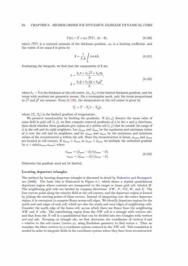
94 CHAPTER 6. HIGHER-ORDER ICE DYNAMICS: GLISSADE DYNAMICAL CORE
T (r) = T + αT ⟨∇T ⟩ · (r− r), (6.120)
where ⟨∇T ⟩ is a centered estimate of the thickness gradient, αT is a limiting coefficient, andthe center of ice mass r is given by
r =1
h A
∫A
h r dA. (6.121)
Evaluating the integrals, we find that the components of r are
x =hcx+ hxx2 + hyxy
h,
y =hcy + hxxy + hyy2
h.
(6.122)
where hc = h is the thickness at the cell center, (hx, hy) is the limited thickness gradient, and theterms with overbars are geometric means. On a rectangular mesh, only the terms proportionalto x2 and y2 are nonzero. From (6.120), the temperature at the cell center is given by
Tc = T − Txx− Ty y,
where (Tx, Ty) is the limited gradient of temperature.We preserve monotonicity by limiting the gradients. If ϕ(i, j) denotes the mean value of
some field in grid cell (i, j), we first compute centered gradients of ϕ in the x and y directions,then check whether these gradients give values of ϕ within cell (i, j) that lie outside the range ofϕ in the cell and its eight neighbors. Let ϕmax and ϕmin be the maximum and minimum valuesof ϕ over the cell and its neighbors, and let ϕmax and ϕmin be the maximum and minimumvalues of the reconstructed ϕ within the cell. Since the reconstruction is linear, ϕmax and ϕmin
are located at cell corners. If ϕmax > ϕmax or ϕmin < ϕmin, we multiply the unlimited gradientby α = min(αmax, αmin), where
αmax = (ϕmax − ϕ)/(ϕmax − ϕ),
αmin = (ϕmin − ϕ)/(ϕmin − ϕ).(6.123)
Otherwise the gradient need not be limited.
Locating departure triangles
The method for locating departure triangles is discussed in detail by Dukowicz and Baumgard-ner (2000). The basic idea is illustrated in Figure 6.1, which shows a shaded quadrilateraldeparture region whose contents are transported to the target or home grid cell, labeled H.The neighboring grid cells are labeled by compass directions: NW , N , NE, W , and E. Thefour vectors point along the velocity field at the cell corners, and the departure region is formedby joining the starting points of these vectors. Instead of integrating over the entire departureregion, it is convenient to compute fluxes across cell edges. We identify departure regions for thenorth and east edges of each cell, which are also the south and west edges of neighboring cells.Consider the north edge of the home cell, across which there are fluxes from the neighboringNW and N cells. The contributing region from the NW cell is a triangle with vertices abc,and that from the N cell is a quadrilateral that can be divided into two triangles with verticesacd and ade. Focusing on triangle abc, we first determine the coordinates of vertices b andc relative to the cell corner (vertex a), using Euclidean geometry to find vertex c. Then wetranslate the three vertices to a coordinate system centered in the NW cell. This translation isneeded in order to integrate fields in the coordinate system where they have been reconstructed.
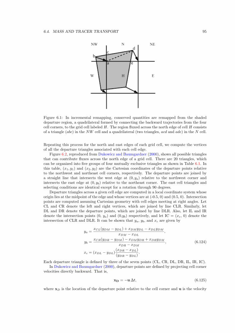
6.4. MASS AND TRACER TRANSPORT 95
Figure 6.1: In incremental remapping, conserved quantities are remapped from the shadeddeparture region, a quadrilateral formed by connecting the backward trajectories from the fourcell corners, to the grid cell labeled H. The region fluxed across the north edge of cell H consistsof a triangle (abc) in the NW cell and a quadrilateral (two triangles, acd and ade) in the N cell.
Repeating this process for the north and east edges of each grid cell, we compute the verticesof all the departure triangles associated with each cell edge.
Figure 6.2, reproduced from Dukowicz and Baumgardner (2000), shows all possible trianglesthat can contribute fluxes across the north edge of a grid cell. There are 20 triangles, whichcan be organized into five groups of four mutually exclusive triangles as shown in Table 6.1. Inthis table, (x1, y1) and (x2, y2) are the Cartesian coordinates of the departure points relativeto the northwest and northeast cell corners, respectively. The departure points are joined bya straight line that intersects the west edge at (0, ya) relative to the northwest corner andintersects the east edge at (0, yb) relative to the northeast corner. The east cell triangles andselecting conditions are identical except for a rotation through 90 degrees.
Departure triangles across a given cell edge are computed in a local coordinate system whoseorigin lies at the midpoint of the edge and whose vertices are at (-0.5, 0) and (0.5, 0). Intersectionpoints are computed assuming Cartesian geometry with cell edges meeting at right angles. LetCL and CR denote the left and right vertices, which are joined by line CLR. Similarly, letDL and DR denote the departure points, which are joined by line DLR. Also, let IL and IRdenote the intersection points (0, ya) and (0,yb) respectively, and let IC = (xc, 0) denote theintersection of CLR and DLR. It can be shown that ya, yb, and xc are given by
ya =xCL(yDM − yDL) + xDMyDL − xDLyDM
xDM − xDL,
yb =xCR(yDR − yDM )− xDMyDR + xDRyDM
xDR − xDM,
xc = (xDL − yDL)(xDR − xDL)
(yDR − yDL).
(6.124)
Each departure triangle is defined by three of the seven points (CL, CR, DL, DR, IL, IR, IC).In Dukowicz and Baumgardner (2000), departure points are defined by projecting cell corner
velocities directly backward. That is,
xD = −u∆t, (6.125)
where xD is the location of the departure point relative to the cell corner and u is the velocity
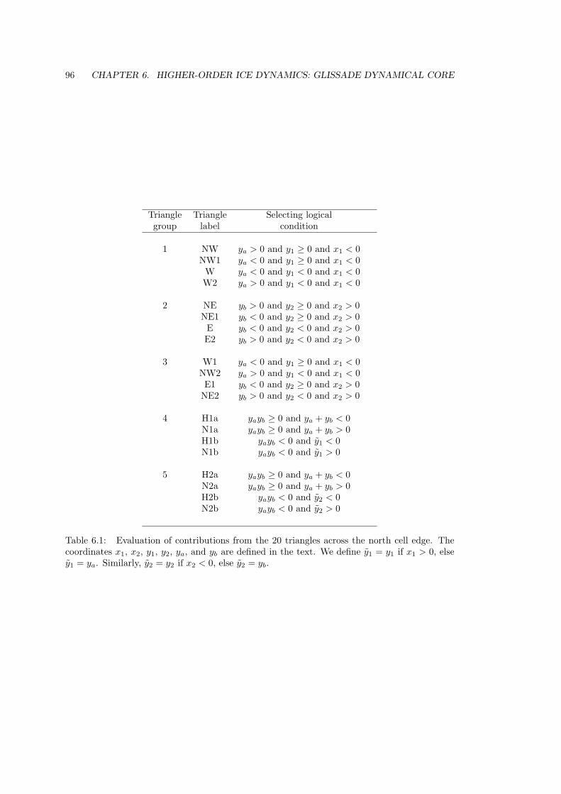
96 CHAPTER 6. HIGHER-ORDER ICE DYNAMICS: GLISSADE DYNAMICAL CORE
Triangle Triangle Selecting logicalgroup label condition
1 NW ya > 0 and y1 ≥ 0 and x1 < 0NW1 ya < 0 and y1 ≥ 0 and x1 < 0W ya < 0 and y1 < 0 and x1 < 0W2 ya > 0 and y1 < 0 and x1 < 0
2 NE yb > 0 and y2 ≥ 0 and x2 > 0NE1 yb < 0 and y2 ≥ 0 and x2 > 0E yb < 0 and y2 < 0 and x2 > 0E2 yb > 0 and y2 < 0 and x2 > 0
3 W1 ya < 0 and y1 ≥ 0 and x1 < 0NW2 ya > 0 and y1 < 0 and x1 < 0E1 yb < 0 and y2 ≥ 0 and x2 > 0NE2 yb > 0 and y2 < 0 and x2 > 0
4 H1a yayb ≥ 0 and ya + yb < 0N1a yayb ≥ 0 and ya + yb > 0H1b yayb < 0 and y1 < 0N1b yayb < 0 and y1 > 0
5 H2a yayb ≥ 0 and ya + yb < 0N2a yayb ≥ 0 and ya + yb > 0H2b yayb < 0 and y2 < 0N2b yayb < 0 and y2 > 0
Table 6.1: Evaluation of contributions from the 20 triangles across the north cell edge. Thecoordinates x1, x2, y1, y2, ya, and yb are defined in the text. We define y1 = y1 if x1 > 0, elsey1 = ya. Similarly, y2 = y2 if x2 < 0, else y2 = yb.
6.4. MASS AND TRACER TRANSPORT 97
Figure 6.2: The 20 possible triangles that can contribute fluxes across the north edge of a gridcell.
at the corner. This approximation is only first-order accurate. In CISM, accuracy is improvedby estimating the velocity at the midpoint of the trajectory.
Integrating fields
Next, we integrate the reconstructed fields over the departure triangles to find the total volumeand internal energy transported across each cell edge. Volume transports are easy to computesince the ice thickness is linear in x and y. Given a triangle with vertices xi = (xi, yi), i ∈1, 2, 3, the triangle area is
AT =1
2|(x2 − x1)(y3 − y1)− (y2 − y1)(x3 − x1)| . (6.126)
The integral Fa of any linear function f(r) over a triangle is given by
Fa = AT f(x0), (6.127)
where x0 = (x0, y0) is the triangle midpoint,
x0 =1
3
3∑i=1
xi. (6.128)
Thus, to compute the volume transport, we evaluate the thickness at the midpoint,
h(x0) = hc + hxx0 + hyy0, (6.129)
and multiply by AT . By convention, northward and eastward transport is positive, while south-ward and westward transport is negative.
Eq. (6.127) cannot be used for energy transport, because the reconstructed internal energyis a quadratic function of position. (It is the product of two linear functions, for thickness
98 CHAPTER 6. HIGHER-ORDER ICE DYNAMICS: GLISSADE DYNAMICAL CORE
and temperature.) The integral of a quadratic polynomial over a triangle requires functionevaluations at three points,
Fh =AT
3
3∑i=1
f (x′i) , (6.130)
where x′i = (x0 + xi)/2 are points lying halfway between the midpoint and the three vertices.
Updating state variables
Finally, we compute new values of the state variables in each ice layer of each grid cell. Thenew ice thickness h′(i, j) is given by
h′(i, j) = h(i, j) +FE(i− 1, j)− FE(i, j) + FN (i, j − 1)− FN (i, j)
A(i, j)(6.131)
where FE(i, j) and FN (i, j) are the volume transports across the east and north edges, re-spectively, of cell (i, j), and A(i, j) is the grid cell area. All transports added to one cell aresubtracted from a neighboring cell; thus (6.131) conserves total ice volume.
The new internal energy in each layer is computed analogously. New temperatures are thengiven by the ratio of energy to volume. (Other tracers, if present, are updated in the same way.)Tracer monotonicity is ensured because
T ′ =
∫AhT dA∫
Ah dA
,
where T ′ is the new-time temperature, given by integrating the old-time thickness and temper-ature over a Lagrangian departure region with area A. That is, the new-time temperature is aweighted averages over old-time values, with non-negative weights h. Thus the new-time valuesmust lie between the maximum and minimum of the old-time values.
6.4.2 CFL checks
As mentioned above, the time step used for explicit advection is limited by the advective CFLcondition (6.116). Furthermore, for ice flux parallel to ∇s, ice thickness evolution is diffusive,giving rise to an additional diffusive CFL condition (Bueler and Brown, 2009):
(maxD)∆t ≤ 0.5∆x2 (6.132)
Flow governed by the shallow-ice approximation is always subject to this diffusive CFL, butsome component of higher-order flow may not be because the ice velocity may not be parallelto ∇s (Bueler and Brown, 2009).
For these reasons, Glissade’s transport scheme checks both the advective and diffusive CFLconditions and writes a warning to the log file if either is violated. These warnings indicate thei, j indices (on the global domain) of the point where the worst violation occurred, as well asthe maximum allowable time step given the CFL condition(s).
The diffusivity is approximated using the component of velocity in the downslope direction:
D =(u · ∇s)H
|∇s|(6.133)
Future work may identify a less restrictive diffusivity, so the diffusive CFL warnings currentlywritten may be overly restrictive. In other words, it is possible for a stable simulation to generatea diffusive CFL warning.
Advective CFL violations generally lead to stability problems with thickness evolution. How-ever, since CFL violations may occur in portions of the domain that are not of interest to the
6.5. BASAL PHYSICS 99
user, these violations are not set to be a fatal error. Note, however, that the IR scheme maygenerate a “departure points out of bounds” error when advective CFL violations occur. Thisis a failure in the method that does result in a fatal error.
Eventually, CISM may include an adaptive time-stepping scheme that adjusts the time stepbased on the advective and diffusive CFL conditions. At present, however, the time step must beset manually and remain constant over a simulation. To aid in determining an appropriate timestep, the adv cfl dt and diff cfl dt variables can be added to an output file. These variablesare the maximum allowable time steps at each time in the model based on the advective anddiffusive CFL conditions, respectively. In some cases, stability might require taking half of thereported values.
6.5 Basal physics
Glissade assumes a basal friction law of the form
τb = βub, (6.134)
where ub is the basal velocity, τb is the basal shear stress, and β > 0. If β were independentof velocity, then (6.26) would be a simple linear sliding law. Allowing β to depend on velocity,however, allows more complex and physically realistic sliding laws.
The sliding law used by Glissade is determined by the value of which ho babc. The followingoptions are supported:
• Spatially uniform β.
• Very slow sliding, enforced by setting β to a large value of 1010 Pa yr/m. This is a specialcase of spatially uniform β and is the default.
• No sliding, enforced by a Dirichlet boundary condition ub = 0 during finite-elementassembly.
• A 2D β field specified from an external file. Typically, β is chosen at each vertex tooptimize the fit to a surface velocity data set.
• β is set to a large value where the bed is frozen (Tb < Tpmp) and a lower value where thebed is thawed (Tb = Tpmp).
• Power-law sliding, based on the classic sliding relation of Weertman (1957). Basal velocityis given by
ub = kτpbN−q, (6.135)
where N is the effective pressure (the difference between the ice overburden pressure andthe basal water pressure) and k is an empirical constant. This can be rearranged to give
τb = k−1/pNq/pub1/p, (6.136)
which determines the form of β. Following Cuffey and Paterson (2010), the default expo-nents are p = 3 and q = 1.
• Coulomb friction, as described by Schoof (2005), with notation and default values fromPimentel et al. (2010). The form of the sliding law is
τb = C|u|1n−1
u
(Nn
κ |u|+Nn
) 1n
(6.137)
100 CHAPTER 6. HIGHER-ORDER ICE DYNAMICS: GLISSADE DYNAMICAL CORE
where C is a dimensionless constant, κ = mmax/(λmaxAb), mmax is the maximum bedobstacle slope, λmax is the wavelength of bedrock bumps, and Ab is a basal flow-lawparameter. The default values are C = 0.42, mmax = 0.5, λmax = 2.0 m, and Ab =10−16 Pa−n m−1.
Eq. (6.137) has two asymptotic behaviors. In the interior, where the ice is thick andslow-moving, κ |u| ≪ Nn and the basal friction is independent of N :
τb ≈ C|u|1n−1
u, (6.138)
In the Coulomb-friction limit, where the ice is thin and fast-moving, κ |u| ≫ Nn, giving
τb ≈C
κ1n
Nu
|u|. (6.139)
• Pseudo-plastic sliding, as described by Aschwanden et al. (2013) and implemented in theParallel Ice Sheet Model (PISM). The basal friction law is
τb = −τcub
|ub|1−quq0
, (6.140)
where τc is the yield stress, q is a pseudo-plastic exponent (default = 0.5), and u0 is athreshold speed (default = 100 m/yr). This law incorporates linear (q = 1), plastic (q = 0)and power-law (0 < q < 1) behavior in a single expression. The yield stress is proportionalto effective pressure:
τc = tan(ϕ)N, (6.141)
where ϕ is a friction angle that can vary with bed elevation. Following Aschwanden et al.(2016), the default is to set ϕ = 5 at elevations more than 700 m below sea level andϕ = 40 at elevations more than 700 m above sea level, with a linear ramp in between.
The power-law, Coulomb-friction and pseudo-plastic sliding laws give lower friction andfaster sliding as the effective pressure N decreases from the overburden pressure to lower values.CISM offers several options for computing N at the bed:
• N = ρigH, the full overburden pressure. That is, the water pressure pw = 0 at the bed.
• N is reduced as the basal temperature approaches the pressure melting point, reaching asmall fraction of overburden pressure (typically δ = 0.02) when T = Tpmp.
• N is reduced as the basal water depth increases, reaching a small fraction of overburdenpressure when the water depth exceeds a prescribed threshold. (This option is of limiteduse, however, since CISM does not yet have a realistic basal hydrology model.)
• Following Leguy et al. (2014), N is reduced where the bed is below sea level, to account forpartial or full connectivity of the basal water system to the ocean. The effective pressureis given by
N = ρigH
(1− Hf
H
)p
, (6.142)
where Hf = max(0, ρw
ρib)is the flotation thickness, b is the depth of the bed, and 0 ≤
p ≤ 1. For p = 0 there is no connectivity and N is the full overburden pressure. For p = 1there is full connectivity, and the basal water pressure is equal to the ocean pressure atthe same depth.
6.6. CALVING 101
6.6 Calving
Glide includes several simple schemes for iceberg calving. Three of these schemes are supportedin Glissade:
• Calve all floating ice.
• Calve ice where the current bedrock lies below a certain elevation.
• Calve ice where the relaxed bedrock (i.e., the bedrock toward which a viscous astheno-sphere is relaxing) lies below a certain elevation.
In addition, there is a more complex scheme to calve floating ice thinner than a user-definedthreshold HC . As discussed by Albrecht et al. (2011), this is not as simple as it sounds. SupposeHC = 100 m, and an ice shelf with ice thicker than 100 m is advancing. During the next timestep, ice will be transported to grid cells just downstream of the initial calving front. Providedthe time step is not too long, these cells will have H < HC . If this thin ice immediately calves,then the calving front cannot advance.
Glissade avoids this problem by defining a protected ring of thin ice at the margin of floatingice. If ice in a grid cell has H < HC but shares an edge with a cell where H ≥ HC , then itis protected from calving. It can then thicken due to transport from neighboring cells, whileremaining dynamically inactive. Once the ice in this cell thickens to H ≥ HC , it becomesdynamically active, and its thin-ice neighbors become part of the protected ring.
Suppose, on the other hand, that ice is thinning at the calving front. A cell might initiallyhave H ≥ HC , with one or more protected thin-ice neighbors. If the ice in this cell thins toH < HC , it becomes a dynamically inactive cell in the protected ring. Its thin-ice neighbors(assuming they have no other neighbors with H ≥ HC) are no longer protected and are allowedto calve. In this way the calving front can retreat.
The thickness-based calving scheme is more realistic than the simple schemes listed above,but still is likely to give large errors in calving-front location. A more accurate damage-basedscheme is under development and will be included in future versions of CISM. In this scheme,a scalar damage parameter evolves as the ice undergoes strain, and ice calves when the damagein a grid cell exceeds a prescribed threshold.
By default, any floating ice that meets the calving criterion (e.g., it is thin and lies outsidethe protected ring, or the bedrock topography lies below the threshold elevation) will calve ona given time step. A user might prefer, however, to limit the extent of calving. By changingthe value of calving domain, the user can specify that ice calves (1) only when it lies at themarine margin (i.e., it borders an ice-free ocean cell), or (2) only when it is connected to theocean through other cells that meet the calving criterion. In this way, cells in the interior of anice shelf can be prevented from calving.
The user can also prescribe a calving timescale. If this timescale is longer than the modeltime step, then only a fraction of the ice that meets the calving criterion will calve in a singletime step. For example, if the model time step is 1 yr and the calving timescale is 2 yr, thenhalf the ice thickness in each calving-eligible cell will calve.
A related option is to remove so-called floating ice islands. A floating island is a connectedregion where every cell is floating and thus has no basal traction. These islands can be present ininitial data sets or can arise occasionally during simulations, depending on the calving scheme.Finding the velocity for such a region is an ill-posed problem, so it is best to remove floatingislands as soon as they occur. This is done by first marking all the grounded ice cells, and thenusing a boundary-fill algorithm to mark every cell that is connected to a grounded cell. (That is,one could travel from a grounded cell to the cell in question along a path at least one cell wide,without leaving the ice pack.) For parallel simulations, the algorithm is repeated enough timesto connect cells on all processors. Any floating cells remaining are ice islands that immediatelycalve.
102 CHAPTER 6. HIGHER-ORDER ICE DYNAMICS: GLISSADE DYNAMICAL CORE
When CISM is coupled to a climate model, calving ice is typically routed to the ocean as asolid ice flux. In the absence of an explicit iceberg model, the ocean model supplies the heatneeded to melt the ice. The ocean cools and freshens accordingly.
6.7 Other model physics
The Glissade modules for velocity, temperature, transport, and calving replace the correspond-ing Glide modules when dycore = 2 is set in the config file. Other model physics, however,remains similar to Glide. In particular:
• Isostasy is treated in the same way as in Glide (see Section 4.4). The lithosphere can betreated as local or elastic, and the asthenosphere is either fluid or relaxing. The elasticlithosphere calculation is non-local and has not been parallelized. Thus it is not possibleto simulate an elastic lithosphere when running on more than one processor.
• Typically, the geothermal heat flux is set to a constant or prescribed from an input file. Asin Glide, however, it is also possible to compute the geothermal heat flux from a model ofheat flow in bedrock (see Section 4.3.2). This model includes non-local horizontal diffusionwhich, like the elastic lithosphere, has not been parallelized and therefore will not workon multiple processors.
• The basal water options in Glissade are also the same as those in Glide. These are all localexcept for basal water = 2, which computes a flux of basal water based on a steady-staterouting calculation. The routing calculation is not parallel and has not been tested withGlissade.
A sophisticated basal hydrology model is under development and will likely be included infuture versions of CISM. This model will output the effective pressure, which is a required inputfor the Coulomb friction law (which ho babc = 10) recently introduced in CISM. For now theeffective pressure is either read from an input file or parameterized simply (using basal water
= 4). The Coulomb friction law is not yet scientifically supported and should be used at yourown risk.
In summary, although CISM has a sophisticated higher-order dycore, the physics parame-terizations remain fairly simple, especially for runs with multiple processors. This is an area ofactive development.
Chapter 7
Running CISM
7.1 Overview of Running CISM
Assuming you successfully completed the Installation instructions in Chapter 2, the executablefor running the model, cism driver, can be found in your build directory in a subdirectorycalled cism driver (e.g., ./builds/mac-gnu/cism driver/cism driver).
The build system creates the executable at this path but does not automatically make itavailable to other locations on your system. How you choose to do so depends on your situation.See the introduction to Chapter 8 for an overview of how to make the executable available toother locations on your system (e.g., symlinking, copying, or modifying your PATH environmentvariable).
CISM2.1 runs with a single executable, cism driver, for all configurations. cism driver
can be invoked with a single argument specifying a CISM .config file to run CISM as a standaloneice sheet model without Glint climate forcing, or with two arguments (a CISM config file and aGlint config file) to run CISM with Glint climate forcing:
Call cism_driver with either 1 or 2 arguments. Examples:
cism_driver ice_sheet.config
cism_driver ice_sheet.config climate.config
The available options for the CISM configuration file and for the Glint climate interface config-uration file are described in detail below.
To perform a parallel run with the parallel build of CISM, you must use the MPI runcommand, which is typically mpirun or mpiexec but may vary among MPI versions and instal-lations. A standard syntax that is likely to work on most installations is
mpirun -np N cism driver ice sheet.config climate.config
where N is the number of processors you want to use, ice sheet.config is the name of theCISM configuration file, and the optional argument climate.config is the name of the climateconfiguration file. For example:
mpirun -np 4 cism driver dome.config
would run the dome test case on four processors.When CISM runs, some basic information about its operation will be output to the screen
(standard out). More verbose information about the run will be written to a log file which isnamed ice sheet.config.log, where ice sheet.config is the name of the .config file usedto perform the run. (For example, if running the model with ./cism driver dome.config,the log file will be called dome.config.log.) The log file is an important reference, especiallyfor debugging runs that do not behave as expected. For example, this file includes a list ofconfiguration options and parameter values, which can be useful in diagnosing problems liketypos in your .config file. The log file also indicates what files were used for input and output and
103
104 CHAPTER 7. RUNNING CISM
at which times I/O occurred. The log file may contain warnings about potentially problematicconfiguration combinations or model behavior, such as the use of configurations settings thatare not scientifically validated, or a CFL violation during advection. In contrast, fatal errorswill kill the model and the error message will be written to both the screen and the log file.
Optionally, the log file also contains diagnostic information about the global state of the icesheet (e.g., the total ice area and volume, the maximum surface and basal speeds, and the maxand min temperatures), along with vertical profiles of speed and temperature at a user-specifiedgrid point. This information is written at intervals specified by the config file variable dt diag,for the diagnostic point (idiag,jdiag).
In addition to the log file, the model will create any netCDF output files requested in theconfig file (see Section 7.4 below for details). If the model dies for some reason midway througha simulation, the netCDF files will still include output for the part of the simulation that wascompleted.
CISM2 (like its predecessor, Glimmer-CISM) has been coupled to the Community EarthSystem Model1 and will be included in future CESM releases. Lipscomb et al. (2013) describedthe initial implementation of CISM in CESM, with one-way forcing of the Greenland ice sheet(using the shallow-ice approximation) by the surface mass balance computed in CESM’s landmodel. Interactive coupling between ice sheets and other climate components has recently beenimplemented and is now being tested. This document, however, does not provide instructionsfor running CISM within CESM or other climate models. Please see here2 for guidance onrunning CISM in CESM.
7.2 Overview of Configuration Files
Running CISM is managed through configuration files (*.config) that enable desired modelfeatures and control input of initial conditions and forcing and output of model results. Thischapter summarizes the configuration options available for running CISM and is divided intosections on general Model Configuration, Input/Ouput Configuration, and optional ClimateForcing Configuration.
The format of CISM configuration files is taken from that used by the ConfigParser modulein Python 2.x, which is similar to Windows .ini files and contains sections. Each sectioncontains key/value pairs.
Comments: Empty lines, or lines starting with a #, ; or ! are ignored. Comments can also be addedon the same line as a key/value pair using these delimiters.
Sections: A new section starts with the section name enclosed by square brackets, [ ] and can beup to 50 characters long, e.g., [grid].
Key/Value Pairs: Keys are separated from their associated values by = or :. The names can be up to 50characters long. Values can be up to 400 characters long.
Sections and keys are case-sensitive and may contain white space. However, the configurationparser is very simple and thus the number of spaces within a key or section name also matters.Sensible defaults are used when a specific key is not found; defaults are shown in bold in thetables below.
Here is an example configuration file:
;a comment
[a section]
an_int : 1
1www2.cesm.ucar.edu2http://www.cesm.ucar.edu/models/cesm2/land-ice/
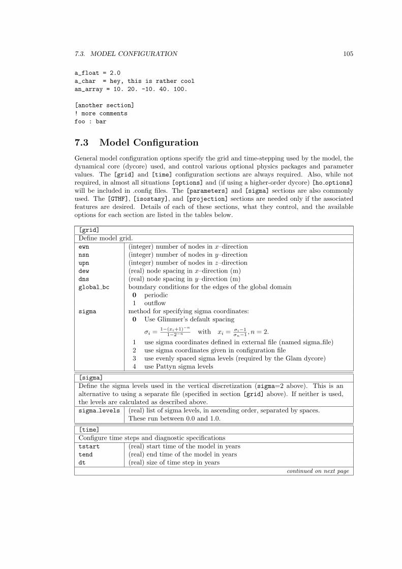
7.3. MODEL CONFIGURATION 105
a_float = 2.0
a_char = hey, this is rather cool
an_array = 10. 20. -10. 40. 100.
[another section]
! more comments
foo : bar
7.3 Model Configuration
General model configuration options specify the grid and time-stepping used by the model, thedynamical core (dycore) used, and control various optional physics packages and parametervalues. The [grid] and [time] configuration sections are always required. Also, while notrequired, in almost all situations [options] and (if using a higher-order dycore) [ho options]
will be included in .config files. The [parameters] and [sigma] sections are also commonlyused. The [GTHF], [isostasy], and [projection] sections are needed only if the associatedfeatures are desired. Details of each of these sections, what they control, and the availableoptions for each section are listed in the tables below.
[grid]
Define model grid.ewn (integer) number of nodes in x–directionnsn (integer) number of nodes in y–directionupn (integer) number of nodes in z–directiondew (real) node spacing in x–direction (m)dns (real) node spacing in y–direction (m)global bc boundary conditions for the edges of the global domain
0 periodic1 outflow
sigma method for specifying sigma coordinates:0 Use Glimmer’s default spacing
σi =1−(xi+1)−n
1−2−n with xi =σi−1σn−1 , n = 2.
1 use sigma coordinates defined in external file (named sigma file)2 use sigma coordinates given in configuration file3 use evenly spaced sigma levels (required by the Glam dycore)4 use Pattyn sigma levels
[sigma]
Define the sigma levels used in the vertical discretization (sigma=2 above). This is analternative to using a separate file (specified in section [grid] above). If neither is used,the levels are calculated as described above.sigma levels (real) list of sigma levels, in ascending order, separated by spaces.
These run between 0.0 and 1.0.
[time]
Configure time steps and diagnostic specificationststart (real) start time of the model in yearstend (real) end time of the model in yearsdt (real) size of time step in years
continued on next page
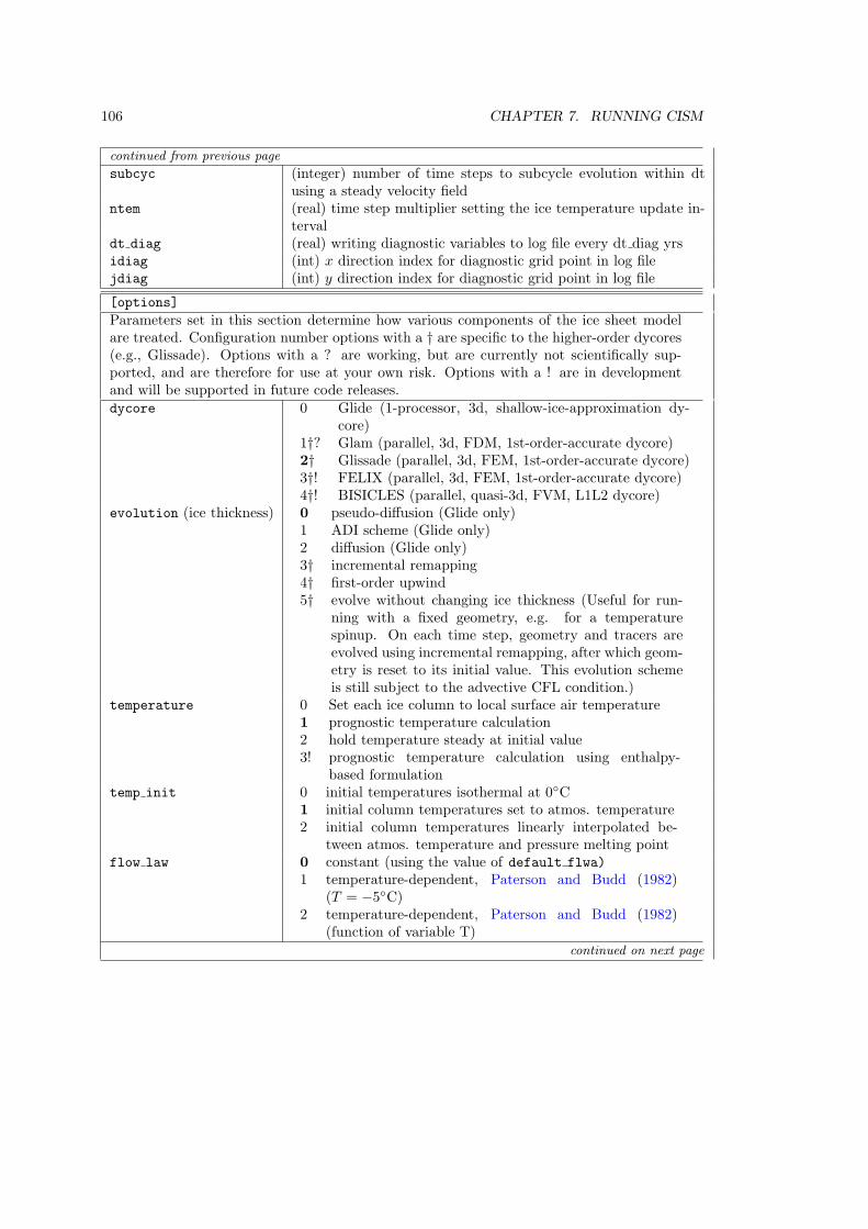
106 CHAPTER 7. RUNNING CISM
continued from previous page
subcyc (integer) number of time steps to subcycle evolution within dtusing a steady velocity field
ntem (real) time step multiplier setting the ice temperature update in-terval
dt diag (real) writing diagnostic variables to log file every dt diag yrsidiag (int) x direction index for diagnostic grid point in log filejdiag (int) y direction index for diagnostic grid point in log file
[options]
Parameters set in this section determine how various components of the ice sheet modelare treated. Configuration number options with a † are specific to the higher-order dycores(e.g., Glissade). Options with a ? are working, but are currently not scientifically sup-ported, and are therefore for use at your own risk. Options with a ! are in developmentand will be supported in future code releases.dycore 0 Glide (1-processor, 3d, shallow-ice-approximation dy-
core)1†? Glam (parallel, 3d, FDM, 1st-order-accurate dycore)2† Glissade (parallel, 3d, FEM, 1st-order-accurate dycore)3†! FELIX (parallel, 3d, FEM, 1st-order-accurate dycore)4†! BISICLES (parallel, quasi-3d, FVM, L1L2 dycore)
evolution (ice thickness) 0 pseudo-diffusion (Glide only)1 ADI scheme (Glide only)2 diffusion (Glide only)3† incremental remapping4† first-order upwind5† evolve without changing ice thickness (Useful for run-
ning with a fixed geometry, e.g. for a temperaturespinup. On each time step, geometry and tracers areevolved using incremental remapping, after which geom-etry is reset to its initial value. This evolution schemeis still subject to the advective CFL condition.)
temperature 0 Set each ice column to local surface air temperature1 prognostic temperature calculation2 hold temperature steady at initial value3! prognostic temperature calculation using enthalpy-
based formulationtemp init 0 initial temperatures isothermal at 0C
1 initial column temperatures set to atmos. temperature2 initial column temperatures linearly interpolated be-
tween atmos. temperature and pressure melting pointflow law 0 constant (using the value of default flwa)
1 temperature-dependent, Paterson and Budd (1982)(T = −5C)
2 temperature-dependent, Paterson and Budd (1982)(function of variable T)
continued on next page
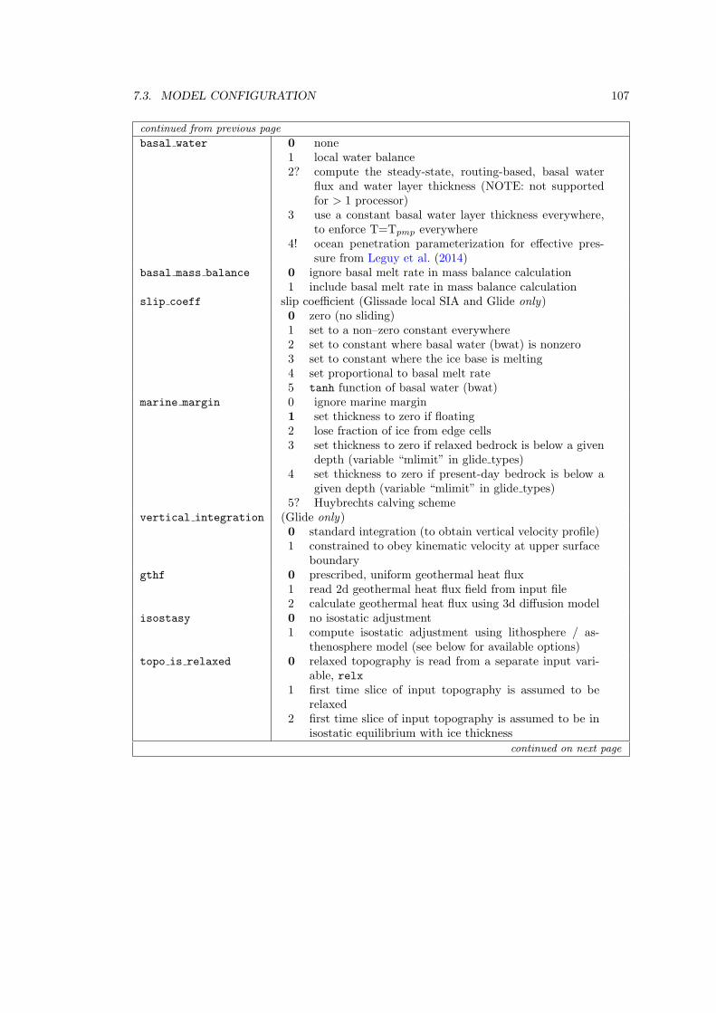
7.3. MODEL CONFIGURATION 107
continued from previous page
basal water 0 none1 local water balance2? compute the steady-state, routing-based, basal water
flux and water layer thickness (NOTE: not supportedfor > 1 processor)
3 use a constant basal water layer thickness everywhere,to enforce T=Tpmp everywhere
4! ocean penetration parameterization for effective pres-sure from Leguy et al. (2014)
basal mass balance 0 ignore basal melt rate in mass balance calculation1 include basal melt rate in mass balance calculation
slip coeff slip coefficient (Glissade local SIA and Glide only)0 zero (no sliding)1 set to a non–zero constant everywhere2 set to constant where basal water (bwat) is nonzero3 set to constant where the ice base is melting4 set proportional to basal melt rate5 tanh function of basal water (bwat)
marine margin 0 ignore marine margin1 set thickness to zero if floating2 lose fraction of ice from edge cells3 set thickness to zero if relaxed bedrock is below a given
depth (variable “mlimit” in glide types)4 set thickness to zero if present-day bedrock is below a
given depth (variable “mlimit” in glide types)5? Huybrechts calving scheme
vertical integration (Glide only)0 standard integration (to obtain vertical velocity profile)1 constrained to obey kinematic velocity at upper surface
boundarygthf 0 prescribed, uniform geothermal heat flux
1 read 2d geothermal heat flux field from input file2 calculate geothermal heat flux using 3d diffusion model
isostasy 0 no isostatic adjustment1 compute isostatic adjustment using lithosphere / as-
thenosphere model (see below for available options)topo is relaxed 0 relaxed topography is read from a separate input vari-
able, relx1 first time slice of input topography is assumed to be
relaxed2 first time slice of input topography is assumed to be in
isostatic equilibrium with ice thicknesscontinued on next page
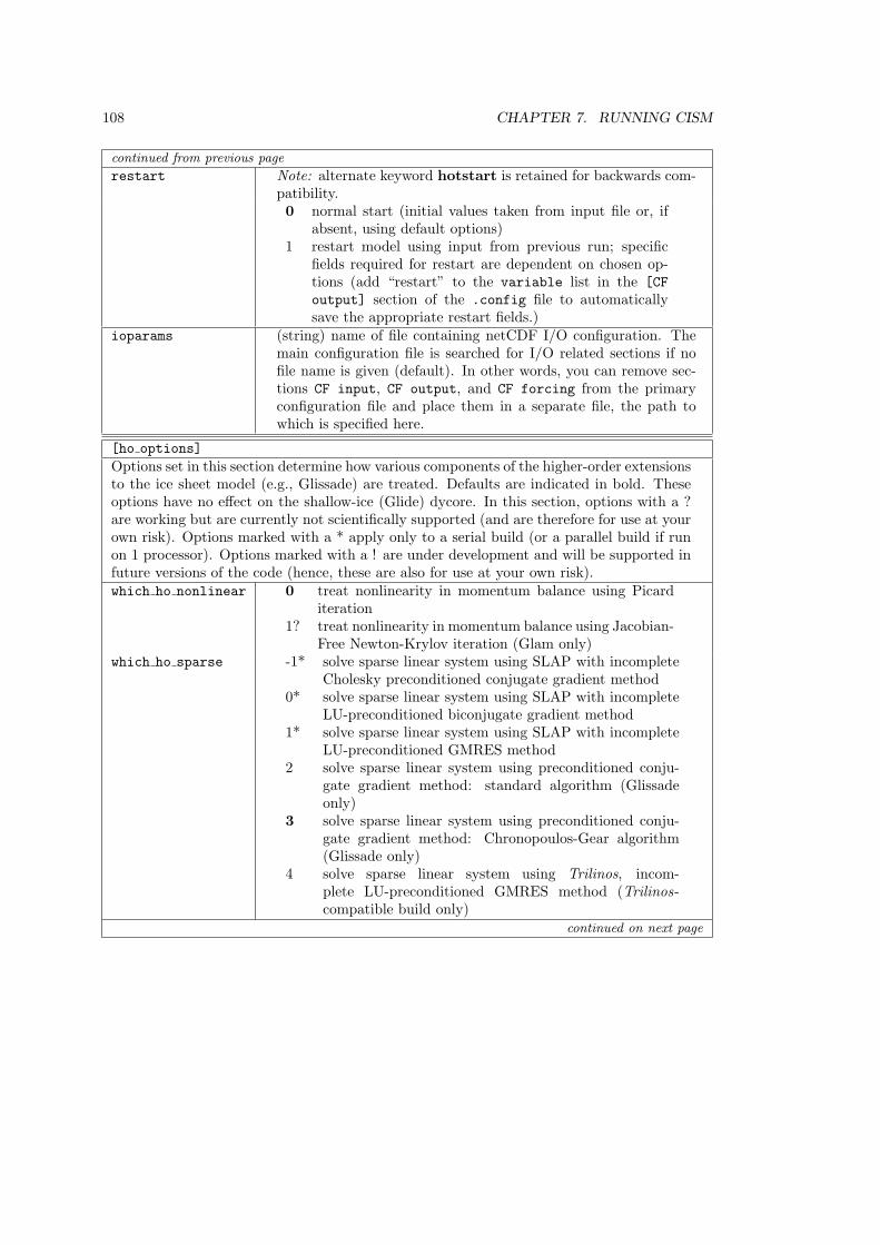
108 CHAPTER 7. RUNNING CISM
continued from previous page
restart Note: alternate keyword hotstart is retained for backwards com-patibility.0 normal start (initial values taken from input file or, if
absent, using default options)1 restart model using input from previous run; specific
fields required for restart are dependent on chosen op-tions (add “restart” to the variable list in the [CF
output] section of the .config file to automaticallysave the appropriate restart fields.)
ioparams (string) name of file containing netCDF I/O configuration. Themain configuration file is searched for I/O related sections if nofile name is given (default). In other words, you can remove sec-tions CF input, CF output, and CF forcing from the primaryconfiguration file and place them in a separate file, the path towhich is specified here.
[ho options]
Options set in this section determine how various components of the higher-order extensionsto the ice sheet model (e.g., Glissade) are treated. Defaults are indicated in bold. Theseoptions have no effect on the shallow-ice (Glide) dycore. In this section, options with a ?are working but are currently not scientifically supported (and are therefore for use at yourown risk). Options marked with a * apply only to a serial build (or a parallel build if runon 1 processor). Options marked with a ! are under development and will be supported infuture versions of the code (hence, these are also for use at your own risk).which ho nonlinear 0 treat nonlinearity in momentum balance using Picard
iteration1? treat nonlinearity in momentum balance using Jacobian-
Free Newton-Krylov iteration (Glam only)which ho sparse -1* solve sparse linear system using SLAP with incomplete
Cholesky preconditioned conjugate gradient method0* solve sparse linear system using SLAP with incomplete
LU-preconditioned biconjugate gradient method1* solve sparse linear system using SLAP with incomplete
LU-preconditioned GMRES method2 solve sparse linear system using preconditioned conju-
gate gradient method: standard algorithm (Glissadeonly)
3 solve sparse linear system using preconditioned conju-gate gradient method: Chronopoulos-Gear algorithm(Glissade only)
4 solve sparse linear system using Trilinos, incom-plete LU-preconditioned GMRES method (Trilinos-compatible build only)
continued on next page

7.3. MODEL CONFIGURATION 109
continued from previous page
which ho efvs 0 use a constant value for the effective viscosity (i.e., linearviscosity). The default value is 2336041 Pa yr (as usedby ISMIP-HOM Test F).
1 set the effective viscosity to a value based on the flowrate factor: efvs = 0.5 ∗A−1/n
2 use the effective strain rate to compute the effective vis-cosity (i.e., full nonlinear treatment)
which ho disp -1 no dissipation term included in temperature equation0 calculate dissipation in temperature equation assuming
SIA ice dynamics1 calculate dissipation in temperature equation assuming
first-order ice dynamicswhich ho babc Implementation of basal boundary condition in higher-order dy-
core0 constant value of “beta”1 specify a simple pattern for “beta” (hardcoded, mainly
useful for debugging)2 read map of yield stress (in Pa) from input field
“mintauf” to simulate sliding over a plastic subglacialtill (Picard-based solution)
3 calculate “beta” as linear (inverse) function of basal wa-ter thickness
4 (virtually) no slip everywhere in domain (“beta” set tovery large value)
5 read map of “beta” from .nc input file using standardI/O
6 no slip everywhere in domain (using Dirichlet basal BC)7! read map of yield stress (in Pa) from input field
“mintauf” to simulate sliding over a plastic subglacialtill (Newton-based solution)
8* Spatial field of “beta” required for ISMIP-HOM TestC (avoids interpolation error associated with option 5;works for a single processor only)
9! Weertman-style power-law accounting for effective pres-sure (Eq. 5.33)
10! Coulomb friction law (Eq. 5.34)continued on next page
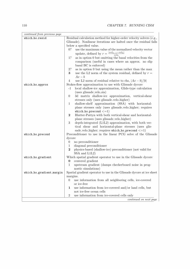
110 CHAPTER 7. RUNNING CISM
continued from previous page
which ho resid Residual calculation method for higher-order velocity solvers (e.g.,Glissade). Nonlinear iterations are halted once the residual fallsbelow a specified value.0? use the maximum value of the normalized velocity vector
update, defined by r = |velk−1−velk|velk
1? as in option 0 but omitting the basal velocities from thecomparison (useful in cases where an approx. no slipbasal BC is enforced)
2? as in option 0 but using the mean rather than the max3 use the L2 norm of the system residual, defined by r =
Ax− b4 use L2 norm of residual relative to rhs, |Ax− b|/|b|
which ho approx Stokes-flow approximation to use with Glissade dycore-1 local shallow-ice approximation, Glide-type calculation
(uses glissade velo sia)0 3d matrix shallow-ice approximation, vertical-shear
stresses only (uses glissade velo higher)1 shallow-shelf approximation (SSA) with horizontal-
plane stresses only (uses glissade velo higher; requireswhich ho precond <=1)
2 Blatter-Pattyn with both vertical-shear and horizontal-plane stresses (uses glissade velo higher)
3 depth-integrated (L1L2) approximation, with both ver-tical shear and horizontal-plane stresses (uses glis-sade velo higher; requires which ho precond <=1)
which ho precond Preconditioner to use in the linear PCG solve of the Glissadedycore0 no preconditioner1 diagonal preconditioner2 physics-based (shallow-ice) preconditioner (not valid for
SSA and L1L2)which ho gradient Which spatial gradient operator to use in the Glissade dycore
0 centered gradient1 upstream gradient (damps checkerboard noise in prog-
nostic simulations)which ho gradient margin Spatial gradient operator to use in the Glissade dycore at ice sheet
margins.0 use information from all neighboring cells, ice-covered
or ice-free1 use information from ice-covered and/or land cells, but
not ice-free ocean cells2 use information from ice-covered cells only
continued on next page
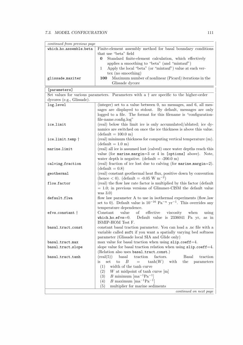
7.3. MODEL CONFIGURATION 111
continued from previous page
which ho assemble beta Finite-element assembly method for basal boundary conditionsthat use “beta” field0 Standard finite-element calculation, which effectively
applies a smoothing to “beta” (and “mintauf”)1 Apply the local “beta” (or “mintauf”) value at each ver-
tex (no smoothing)glissade maxiter 100 Maximum number of nonlinear (Picard) iterations in the
Glissade dycore
[parameters]
Set values for various parameters. Parameters with a † are specific to the higher-orderdycores (e.g., Glissade).log level (integer) set to a value between 0, no messages, and 6, all mes-
sages are displayed to stdout. By default, messages are onlylogged to a file. The format for this filename is “configuration-file-name.config.log”
ice limit (real) below this limit ice is only accumulated/ablated; ice dy-namics are switched on once the ice thickness is above this value.(default = 100.0 m)
ice limit temp † (real) minimum thickness for computing vertical temperature (m).(default = 1.0 m)
marine limit (real) all ice is assumed lost (calved) once water depths reach thisvalue (for marine margin=3 or 4 in [options] above). Note,water depth is negative. (default = -200.0 m)
calving fraction (real) fraction of ice lost due to calving (for marine margin=2).(default = 0.8)
geothermal (real) constant geothermal heat flux, positive down by convention(hence < 0). (default = -0.05 W m−2)
flow factor (real) the flow law rate factor is multiplied by this factor (default= 1.0; in previous versions of Glimmer-CISM the default valuewas 3.0)
default flwa flow law parameter A to use in isothermal experiments (flow lawset to 0). Default value is 10−16 Pa−n yr−1. This overrides anytemperature dependence.
efvs constant † Constant value of effective viscosity when usingwhich ho efvs=0. Default value is 2336041 Pa yr, as inISMIP-HOM Test F.
basal tract const constant basal traction parameter. You can load a .nc file with avariable called soft if you want a spatially varying bed softnessparameter (Glissade local SIA and Glide only)
basal tract max max value for basal traction when using slip coeff=4.basal tract slope slope value for basal traction relation when using slip coeff=4.
(Relation also uses basal tract const.)basal tract tanh (real(5)) basal traction factors. Basal traction
is set to B = tanh(W ) with the parameters(1) width of the tanh curve(2) W at midpoint of tanh curve [m](3) B minimum [ma−1Pa−1](4) B maximum [ma−1Pa−1](5) multiplier for marine sediments
continued on next page
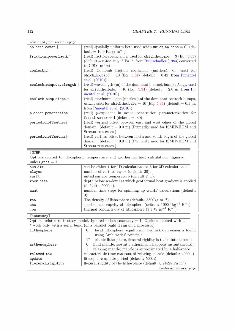
112 CHAPTER 7. RUNNING CISM
continued from previous page
ho beta const † (real) spatially uniform beta used when which ho babc = 0. (de-fault = 10.0 Pa yr m−1)
friction powerlaw k † (real) friction coefficient k used for which ho babc = 9 (Eq. 5.33)(default = 8.4e-9 m y−1 Pa−2, from Bindschadler (1983) convertedto CISM units)
coulomb c † (real) Coulomb friction coefficient (unitless), C, used forwhich ho babc = 10 (Eq. 5.34) (default = 0.42, from Pimentelet al. (2010))
coulomb bump wavelength † (real) wavelength (m) of the dominant bedrock bumps, λmax, usedfor which ho babc = 10 (Eq. 5.34) (default = 2.0 m, from Pi-mentel et al. (2010))
coulomb bump slope † (real) maximum slope (unitless) of the dominant bedrock bumps,mmax, used for which ho babc = 10 (Eq. 5.34) (default = 0.5 m,from Pimentel et al. (2010))
p ocean penetration (real) p-exponent in ocean penetration parameterization for(basal water = 4 (default = 0.0)
periodic offset ew† (real) vertical offset between east and west edges of the globaldomain. (default = 0.0 m) (Primarily used for ISMIP-HOM andStream test cases.)
periodic offset ns† (real) vertical offset between north and south edges of the globaldomain. (default = 0.0 m) (Primarily used for ISMIP-HOM andStream test cases.)
[GTHF]
Options related to lithospheric temperature and geothermal heat calculation. Ignoredunless gthf = 1.num dim can be either 1 for 1D calculations or 3 for 3D calculations.nlayer number of vertical layers (default: 20).surft initial surface temperature (default 2C).rock base depth below sea-level at which geothermal heat gradient is applied
(default: -5000m).numt number time steps for spinning up GTHF calculations (default:
0).rho The density of lithosphere (default: 3300kg m−3).shc specific heat capcity of lithosphere (default: 1000J kg−1 K−1).con thermal conductivity of lithosphere (3.3 W m−1 K−1).
[isostasy]
Options related to isostasy model. Ignored unless isostasy = 1. Options marked with a* work only with a serial build (or a parallel build if run on 1 processor).lithosphere 0 local lithosphere, equilibrium bedrock depression is found
using Archimedes’ principle1* elastic lithosphere, flexural rigidity is taken into account
asthenosphere 0 fluid mantle, isostatic adjustment happens instantaneously1 relaxing mantle, mantle is approximated by a half-space
relaxed tau characteristic time constant of relaxing mantle (default: 4000.a)update lithosphere update period (default: 500.a)flexural rigidity flexural rigidity of the lithosphere (default: 0.24e25 Pa m3)
continued on next page
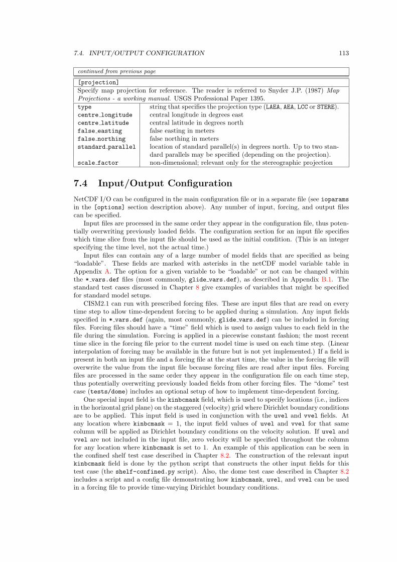
7.4. INPUT/OUTPUT CONFIGURATION 113
continued from previous page
[projection]
Specify map projection for reference. The reader is referred to Snyder J.P. (1987) MapProjections - a working manual. USGS Professional Paper 1395.type string that specifies the projection type (LAEA, AEA, LCC or STERE).centre longitude central longitude in degrees eastcentre latitude central latitude in degrees northfalse easting false easting in metersfalse northing false northing in metersstandard parallel location of standard parallel(s) in degrees north. Up to two stan-
dard parallels may be specified (depending on the projection).scale factor non-dimensional; relevant only for the stereographic projection
7.4 Input/Output Configuration
NetCDF I/O can be configured in the main configuration file or in a separate file (see ioparamsin the [options] section description above). Any number of input, forcing, and output filescan be specified.
Input files are processed in the same order they appear in the configuration file, thus poten-tially overwriting previously loaded fields. The configuration section for an input file specifieswhich time slice from the input file should be used as the initial condition. (This is an integerspecifying the time level, not the actual time.)
Input files can contain any of a large number of model fields that are specified as being“loadable”. These fields are marked with asterisks in the netCDF model variable table inAppendix A. The option for a given variable to be “loadable” or not can be changed withinthe * vars.def files (most commonly, glide vars.def), as described in Appendix B.1. Thestandard test cases discussed in Chapter 8 give examples of variables that might be specifiedfor standard model setups.
CISM2.1 can run with prescribed forcing files. These are input files that are read on everytime step to allow time-dependent forcing to be applied during a simulation. Any input fieldsspecified in * vars.def (again, most commonly, glide vars.def) can be included in forcingfiles. Forcing files should have a “time” field which is used to assign values to each field in thefile during the simulation. Forcing is applied in a piecewise constant fashion; the most recenttime slice in the forcing file prior to the current model time is used on each time step. (Linearinterpolation of forcing may be available in the future but is not yet implemented.) If a field ispresent in both an input file and a forcing file at the start time, the value in the forcing file willoverwrite the value from the input file because forcing files are read after input files. Forcingfiles are processed in the same order they appear in the configuration file on each time step,thus potentially overwriting previously loaded fields from other forcing files. The “dome” testcase (tests/dome) includes an optional setup of how to implement time-dependent forcing.
One special input field is the kinbcmask field, which is used to specify locations (i.e., indicesin the horizontal grid plane) on the staggered (velocity) grid where Dirichlet boundary conditionsare to be applied. This input field is used in conjunction with the uvel and vvel fields. Atany location where kinbcmask = 1, the input field values of uvel and vvel for that samecolumn will be applied as Dirichlet boundary conditions on the velocity solution. If uvel andvvel are not included in the input file, zero velocity will be specified throughout the columnfor any location where kinbcmask is set to 1. An example of this application can be seen inthe confined shelf test case described in Chapter 8.2. The construction of the relevant inputkinbcmask field is done by the python script that constructs the other input fields for thistest case (the shelf-confined.py script). Also, the dome test case described in Chapter 8.2includes a script and a config file demonstrating how kinbcmask, uvel, and vvel can be usedin a forcing file to provide time-varying Dirichlet boundary conditions.
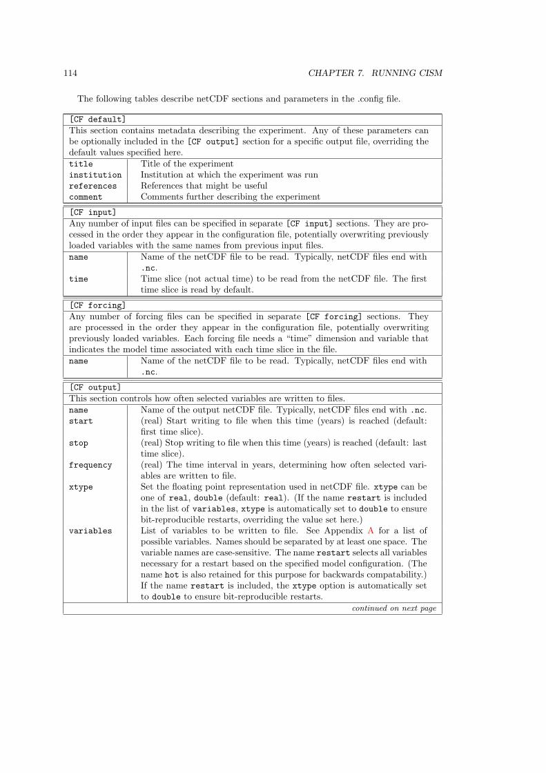
114 CHAPTER 7. RUNNING CISM
The following tables describe netCDF sections and parameters in the .config file.
[CF default]
This section contains metadata describing the experiment. Any of these parameters canbe optionally included in the [CF output] section for a specific output file, overriding thedefault values specified here.title Title of the experimentinstitution Institution at which the experiment was runreferences References that might be usefulcomment Comments further describing the experiment
[CF input]
Any number of input files can be specified in separate [CF input] sections. They are pro-cessed in the order they appear in the configuration file, potentially overwriting previouslyloaded variables with the same names from previous input files.name Name of the netCDF file to be read. Typically, netCDF files end with
.nc.time Time slice (not actual time) to be read from the netCDF file. The first
time slice is read by default.
[CF forcing]
Any number of forcing files can be specified in separate [CF forcing] sections. Theyare processed in the order they appear in the configuration file, potentially overwritingpreviously loaded variables. Each forcing file needs a “time” dimension and variable thatindicates the model time associated with each time slice in the file.name Name of the netCDF file to be read. Typically, netCDF files end with
.nc.
[CF output]
This section controls how often selected variables are written to files.name Name of the output netCDF file. Typically, netCDF files end with .nc.start (real) Start writing to file when this time (years) is reached (default:
first time slice).stop (real) Stop writing to file when this time (years) is reached (default: last
time slice).frequency (real) The time interval in years, determining how often selected vari-
ables are written to file.xtype Set the floating point representation used in netCDF file. xtype can be
one of real, double (default: real). (If the name restart is includedin the list of variables, xtype is automatically set to double to ensurebit-reproducible restarts, overriding the value set here.)
variables List of variables to be written to file. See Appendix A for a list ofpossible variables. Names should be separated by at least one space. Thevariable names are case-sensitive. The name restart selects all variablesnecessary for a restart based on the specified model configuration. (Thename hot is also retained for this purpose for backwards compatability.)If the name restart is included, the xtype option is automatically setto double to ensure bit-reproducible restarts.
continued on next page
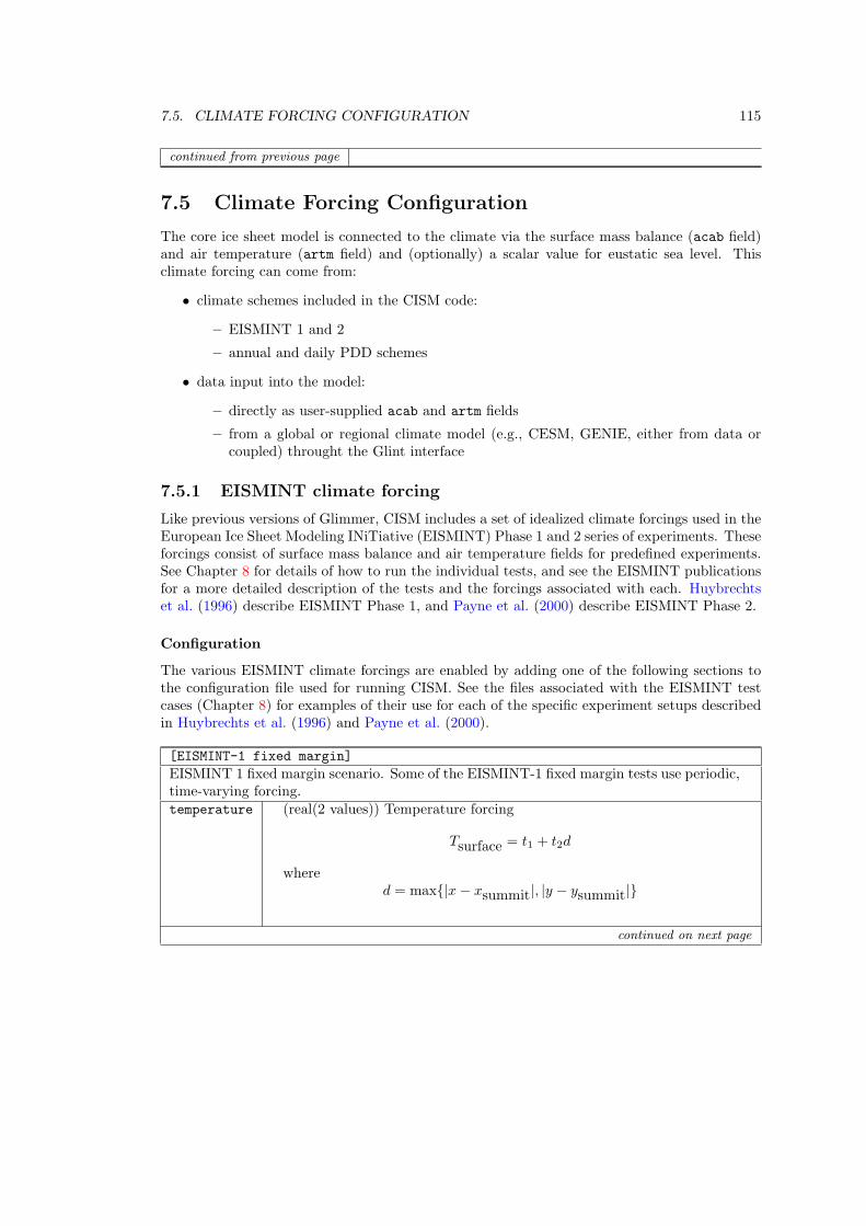
7.5. CLIMATE FORCING CONFIGURATION 115
continued from previous page
7.5 Climate Forcing Configuration
The core ice sheet model is connected to the climate via the surface mass balance (acab field)and air temperature (artm field) and (optionally) a scalar value for eustatic sea level. Thisclimate forcing can come from:
• climate schemes included in the CISM code:
– EISMINT 1 and 2
– annual and daily PDD schemes
• data input into the model:
– directly as user-supplied acab and artm fields
– from a global or regional climate model (e.g., CESM, GENIE, either from data orcoupled) throught the Glint interface
7.5.1 EISMINT climate forcing
Like previous versions of Glimmer, CISM includes a set of idealized climate forcings used in theEuropean Ice Sheet Modeling INiTiative (EISMINT) Phase 1 and 2 series of experiments. Theseforcings consist of surface mass balance and air temperature fields for predefined experiments.See Chapter 8 for details of how to run the individual tests, and see the EISMINT publicationsfor a more detailed description of the tests and the forcings associated with each. Huybrechtset al. (1996) describe EISMINT Phase 1, and Payne et al. (2000) describe EISMINT Phase 2.
Configuration
The various EISMINT climate forcings are enabled by adding one of the following sections tothe configuration file used for running CISM. See the files associated with the EISMINT testcases (Chapter 8) for examples of their use for each of the specific experiment setups describedin Huybrechts et al. (1996) and Payne et al. (2000).
[EISMINT-1 fixed margin]
EISMINT 1 fixed margin scenario. Some of the EISMINT-1 fixed margin tests use periodic,time-varying forcing.temperature (real(2 values)) Temperature forcing
Tsurface = t1 + t2d
whered = max|x− xsummit|, |y − ysummit|
continued on next page
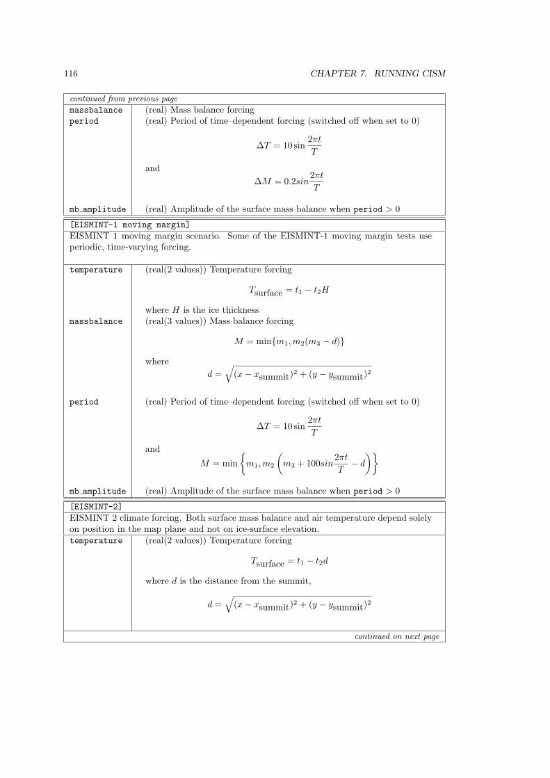
116 CHAPTER 7. RUNNING CISM
continued from previous page
massbalance (real) Mass balance forcingperiod (real) Period of time–dependent forcing (switched off when set to 0)
∆T = 10 sin2πt
T
and
∆M = 0.2sin2πt
T
mb amplitude (real) Amplitude of the surface mass balance when period > 0
[EISMINT-1 moving margin]
EISMINT 1 moving margin scenario. Some of the EISMINT-1 moving margin tests useperiodic, time-varying forcing.
temperature (real(2 values)) Temperature forcing
Tsurface = t1 − t2H
where H is the ice thicknessmassbalance (real(3 values)) Mass balance forcing
M = minm1,m2(m3 − d)
where
d =√
(x− xsummit)2 + (y − ysummit)
2
period (real) Period of time–dependent forcing (switched off when set to 0)
∆T = 10 sin2πt
T
and
M = min
m1,m2
(m3 + 100sin
2πt
T− d
)mb amplitude (real) Amplitude of the surface mass balance when period > 0
[EISMINT-2]
EISMINT 2 climate forcing. Both surface mass balance and air temperature depend solelyon position in the map plane and not on ice-surface elevation.temperature (real(2 values)) Temperature forcing
Tsurface = t1 − t2d
where d is the distance from the summit,
d =√(x− xsummit)
2 + (y − ysummit)2
continued on next page
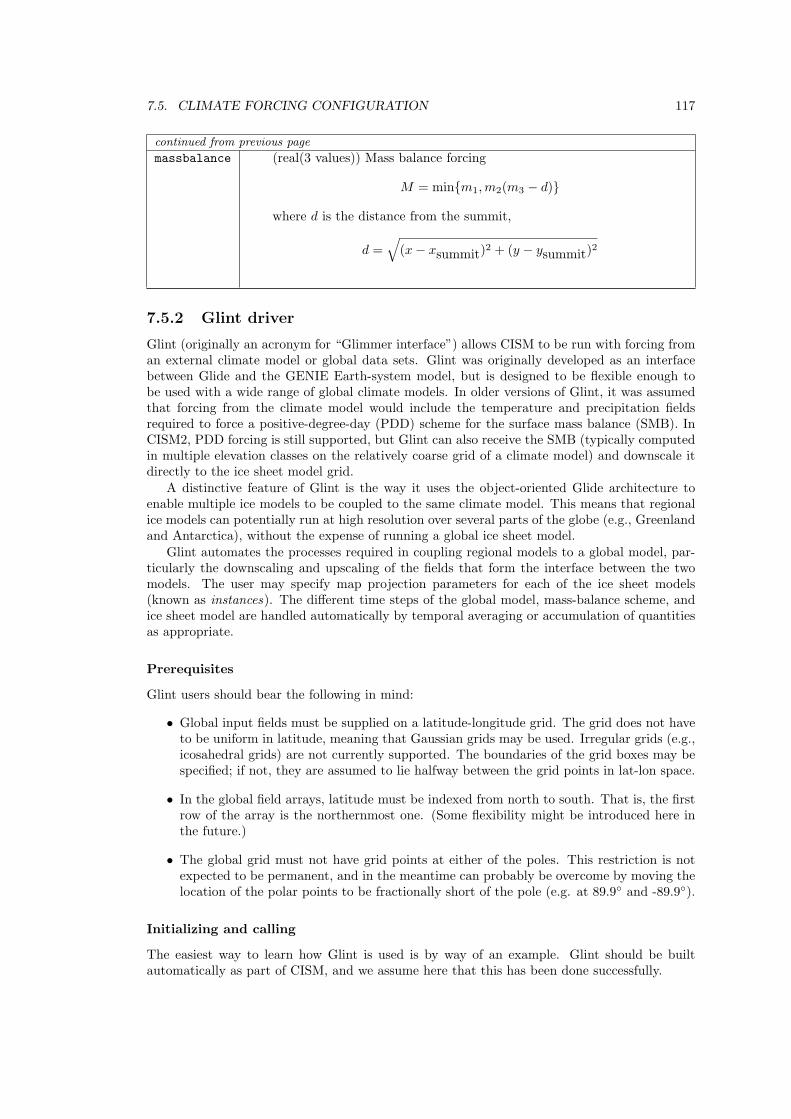
7.5. CLIMATE FORCING CONFIGURATION 117
continued from previous page
massbalance (real(3 values)) Mass balance forcing
M = minm1,m2(m3 − d)
where d is the distance from the summit,
d =√
(x− xsummit)2 + (y − ysummit)
2
7.5.2 Glint driver
Glint (originally an acronym for “Glimmer interface”) allows CISM to be run with forcing froman external climate model or global data sets. Glint was originally developed as an interfacebetween Glide and the GENIE Earth-system model, but is designed to be flexible enough tobe used with a wide range of global climate models. In older versions of Glint, it was assumedthat forcing from the climate model would include the temperature and precipitation fieldsrequired to force a positive-degree-day (PDD) scheme for the surface mass balance (SMB). InCISM2, PDD forcing is still supported, but Glint can also receive the SMB (typically computedin multiple elevation classes on the relatively coarse grid of a climate model) and downscale itdirectly to the ice sheet model grid.
A distinctive feature of Glint is the way it uses the object-oriented Glide architecture toenable multiple ice models to be coupled to the same climate model. This means that regionalice models can potentially run at high resolution over several parts of the globe (e.g., Greenlandand Antarctica), without the expense of running a global ice sheet model.
Glint automates the processes required in coupling regional models to a global model, par-ticularly the downscaling and upscaling of the fields that form the interface between the twomodels. The user may specify map projection parameters for each of the ice sheet models(known as instances). The different time steps of the global model, mass-balance scheme, andice sheet model are handled automatically by temporal averaging or accumulation of quantitiesas appropriate.
Prerequisites
Glint users should bear the following in mind:
• Global input fields must be supplied on a latitude-longitude grid. The grid does not haveto be uniform in latitude, meaning that Gaussian grids may be used. Irregular grids (e.g.,icosahedral grids) are not currently supported. The boundaries of the grid boxes may bespecified; if not, they are assumed to lie halfway between the grid points in lat-lon space.
• In the global field arrays, latitude must be indexed from north to south. That is, the firstrow of the array is the northernmost one. (Some flexibility might be introduced here inthe future.)
• The global grid must not have grid points at either of the poles. This restriction is notexpected to be permanent, and in the meantime can probably be overcome by moving thelocation of the polar points to be fractionally short of the pole (e.g. at 89.9 and -89.9).
Initializing and calling
The easiest way to learn how Glint is used is by way of an example. Glint should be builtautomatically as part of CISM, and we assume here that this has been done successfully.
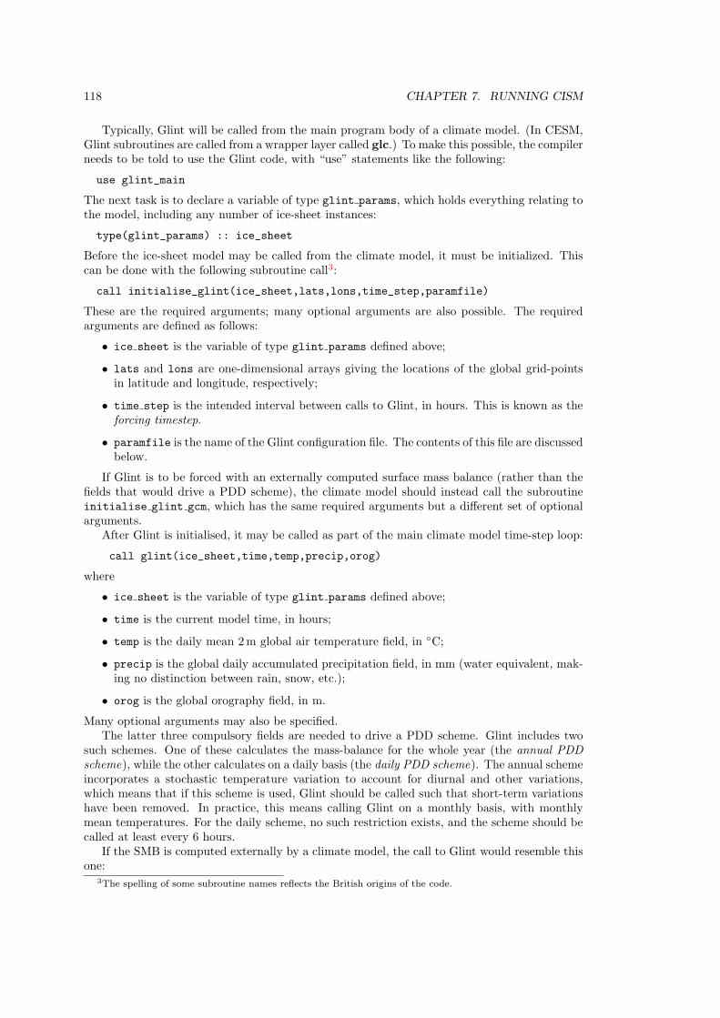
118 CHAPTER 7. RUNNING CISM
Typically, Glint will be called from the main program body of a climate model. (In CESM,Glint subroutines are called from a wrapper layer called glc.) To make this possible, the compilerneeds to be told to use the Glint code, with “use” statements like the following:
use glint_main
The next task is to declare a variable of type glint params, which holds everything relating tothe model, including any number of ice-sheet instances:
type(glint_params) :: ice_sheet
Before the ice-sheet model may be called from the climate model, it must be initialized. Thiscan be done with the following subroutine call3:
call initialise_glint(ice_sheet,lats,lons,time_step,paramfile)
These are the required arguments; many optional arguments are also possible. The requiredarguments are defined as follows:
• ice sheet is the variable of type glint params defined above;
• lats and lons are one-dimensional arrays giving the locations of the global grid-pointsin latitude and longitude, respectively;
• time step is the intended interval between calls to Glint, in hours. This is known as theforcing timestep.
• paramfile is the name of the Glint configuration file. The contents of this file are discussedbelow.
If Glint is to be forced with an externally computed surface mass balance (rather than thefields that would drive a PDD scheme), the climate model should instead call the subroutineinitialise glint gcm, which has the same required arguments but a different set of optionalarguments.
After Glint is initialised, it may be called as part of the main climate model time-step loop:
call glint(ice_sheet,time,temp,precip,orog)
where
• ice sheet is the variable of type glint params defined above;
• time is the current model time, in hours;
• temp is the daily mean 2m global air temperature field, in C;
• precip is the global daily accumulated precipitation field, in mm (water equivalent, mak-ing no distinction between rain, snow, etc.);
• orog is the global orography field, in m.
Many optional arguments may also be specified.The latter three compulsory fields are needed to drive a PDD scheme. Glint includes two
such schemes. One of these calculates the mass-balance for the whole year (the annual PDDscheme), while the other calculates on a daily basis (the daily PDD scheme). The annual schemeincorporates a stochastic temperature variation to account for diurnal and other variations,which means that if this scheme is used, Glint should be called such that short-term variationshave been removed. In practice, this means calling Glint on a monthly basis, with monthlymean temperatures. For the daily scheme, no such restriction exists, and the scheme should becalled at least every 6 hours.
If the SMB is computed externally by a climate model, the call to Glint would resemble thisone:
3The spelling of some subroutine names reflects the British origins of the code.
7.5. CLIMATE FORCING CONFIGURATION 119
call glint_gcm(ice_sheet,time,qsmb,tsrf,topo)
where the last three arguments (all compulsory) are defined as follows:
• qsmb is the surface mass balance in kg m−2 s−1;
• tsrf is the surface ground temperature in C, used as an upper thermal boundary con-dition for the ice sheet; and
• topo is the surface elevation in m.
These fields contain two horizontal dimensions, along with a third dimension for elevation class.CESM typically computes these quantities in 10 elevation classes per glaciated grid cell in theclimate model.
Among the optional arguments are the following output fields (returned by Glint to theclimate model):
• gfrac is the fractional grid cell area covered by ice;
• gtopo is the mean surface elevation in m;
• ghflx is the upwelling heat flux at the ice sheet surface, in W m2;
• grofi is the solid runoff flux (i.e., the calving flux) in kg m−2 s−1;
• grofl is the liquid runoff flux in kg m−2 s−1. This includes basal and possibly internalmelting, but not surface melting (which has already been computed by the climate model).
These fields are required by CESM to update its land-surface types and topography and toconserve heat and water when CISM is coupled interactively to the climate model. The firstthree fields are computed for each elevation class in each climate model grid cell, and the tworunoff fluxes are averaged over each grid cell. The initial “g” denotes that these fields have beenupscaled to the global climate grid.
Finishing off
After the desired number of time steps have been run, Glint may have some tidying up to do.To do this, the subroutine end glint must be called:
call end_glint(ice_sheet)
Configuration
Glint uses the same configuration file format as the rest of CISM. If there is only one ice sheetinstance, all the configuration data for Glint and Glide (or Glissade) can reside in the same file.If two or more instances are used, a top-level file specifies the number of model instances andthe name of a configuration file for each one. Configuration sections specific to Glint are asfollows:
[Glint]
Section specifying number of instances.n instance (integer) Number of instances (default=1)
[Glint instance]
Specifies the name of an instance-specific configuration file. Unnecessary if we only have oneinstance whose configuration data is in the main config file.
continued on next page
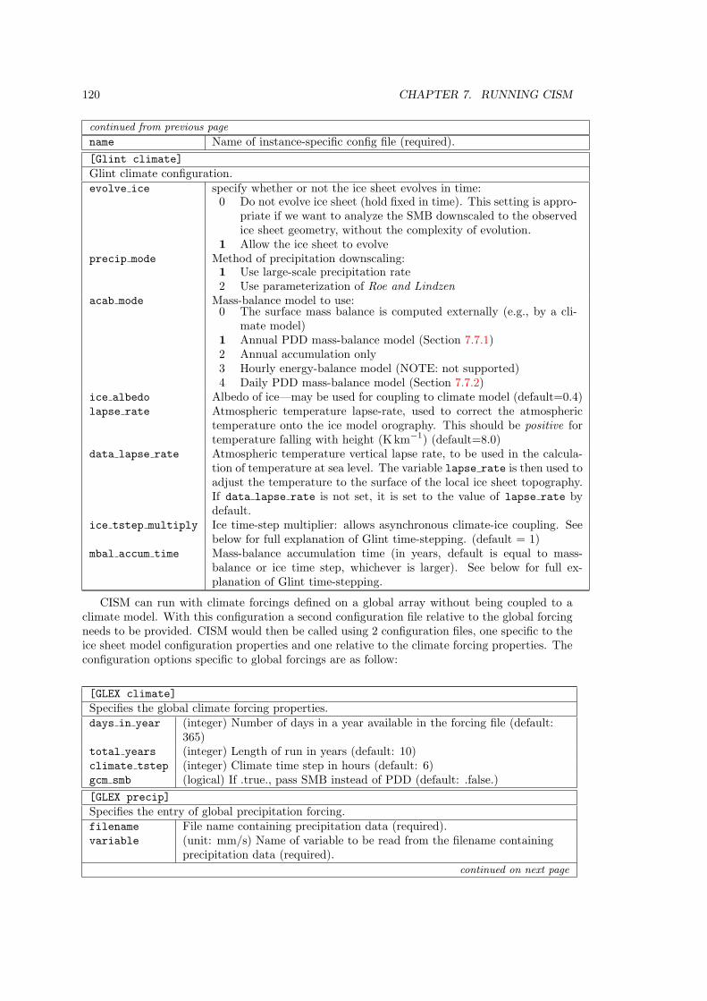
120 CHAPTER 7. RUNNING CISM
continued from previous page
name Name of instance-specific config file (required).
[Glint climate]
Glint climate configuration.evolve ice specify whether or not the ice sheet evolves in time:
0 Do not evolve ice sheet (hold fixed in time). This setting is appro-priate if we want to analyze the SMB downscaled to the observedice sheet geometry, without the complexity of evolution.
1 Allow the ice sheet to evolveprecip mode Method of precipitation downscaling:
1 Use large-scale precipitation rate2 Use parameterization of Roe and Lindzen
acab mode Mass-balance model to use:0 The surface mass balance is computed externally (e.g., by a cli-
mate model)1 Annual PDD mass-balance model (Section 7.7.1)2 Annual accumulation only3 Hourly energy-balance model (NOTE: not supported)4 Daily PDD mass-balance model (Section 7.7.2)
ice albedo Albedo of ice—may be used for coupling to climate model (default=0.4)lapse rate Atmospheric temperature lapse-rate, used to correct the atmospheric
temperature onto the ice model orography. This should be positive fortemperature falling with height (Kkm−1) (default=8.0)
data lapse rate Atmospheric temperature vertical lapse rate, to be used in the calcula-tion of temperature at sea level. The variable lapse rate is then used toadjust the temperature to the surface of the local ice sheet topography.If data lapse rate is not set, it is set to the value of lapse rate bydefault.
ice tstep multiply Ice time-step multiplier: allows asynchronous climate-ice coupling. Seebelow for full explanation of Glint time-stepping. (default = 1)
mbal accum time Mass-balance accumulation time (in years, default is equal to mass-balance or ice time step, whichever is larger). See below for full ex-planation of Glint time-stepping.
CISM can run with climate forcings defined on a global array without being coupled to aclimate model. With this configuration a second configuration file relative to the global forcingneeds to be provided. CISM would then be called using 2 configuration files, one specific to theice sheet model configuration properties and one relative to the climate forcing properties. Theconfiguration options specific to global forcings are as follow:
[GLEX climate]
Specifies the global climate forcing properties.days in year (integer) Number of days in a year available in the forcing file (default:
365)total years (integer) Length of run in years (default: 10)climate tstep (integer) Climate time step in hours (default: 6)gcm smb (logical) If .true., pass SMB instead of PDD (default: .false.)
[GLEX precip]
Specifies the entry of global precipitation forcing.filename File name containing precipitation data (required).variable (unit: mm/s) Name of variable to be read from the filename containing
precipitation data (required).continued on next page
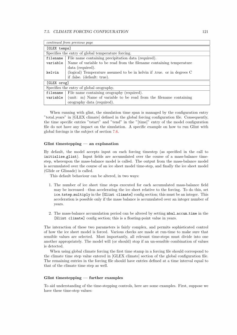
7.5. CLIMATE FORCING CONFIGURATION 121
continued from previous page
[GLEX temps]
Specifies the entry of global temperature forcing.filename File name containing precipitation data (required).variable Name of variable to be read from the filename containing temperature
data (required).kelvin (logical) Temperature assumed to be in kelvin if .true. or in degrees C
if .false. (default: true).
[GLEX orog]
Specifies the entry of global orography.filename File name containing orography (required).variable (unit: m) Name of variable to be read from the filename containing
orography data (required).
When running with glint, the simulation time span is managed by the configuration entry”total years” in [GLEX climate] defined in the global forcing configuration file. Consequently,the time specific entries ”tstart” and ”tend” in the ”[time]” entry of the model configurationfile do not have any impact on the simulation. A specific example on how to run Glint withglobal forcings is the subject of section 7.6.
Glint timestepping — an explanation
By default, the model accepts input on each forcing timestep (as specified in the call toinitialise glint). Input fields are accumulated over the course of a mass-balance time-step, whereupon the mass-balance model is called. The output from the mass-balance modelis accumulated over the course of an ice sheet model time-step, and finally the ice sheet model(Glide or Glissade) is called.
This default behaviour can be altered, in two ways:
1. The number of ice sheet time steps executed for each accumulated mass-balance fieldmay be increased—thus accelerating the ice sheet relative to the forcing. To do this, setice tstep multiply in the [Glint climate] config section; this must be an integer. Thisacceleration is possible only if the mass balance is accumulated over an integer number ofyears.
2. The mass-balance accumulation period can be altered by setting mbal accum time in the[Glint climate] config section; this is a floating-point value in years.
The interaction of these two parameters is fairly complex, and permits sophisticated controlof how the ice sheet model is forced. Various checks are made at run-time to make sure thatsensible values are selected. Most importantly, all relevant time-steps must divide into oneanother appropriately. The model will (or should) stop if an un-sensible combination of valuesis detected.
When using global climate forcing the first time stamp in a forcing file should correspond tothe climate time step value entered in [GLEX climate] section of the global configuration file.The remaining entries in the forcing file should have entries defined at a time interval equal tothat of the climate time step as well.
Glint timestepping — further examples
To aid understanding of the time-stepping controls, here are some examples. First, suppose wehave these time-step values:
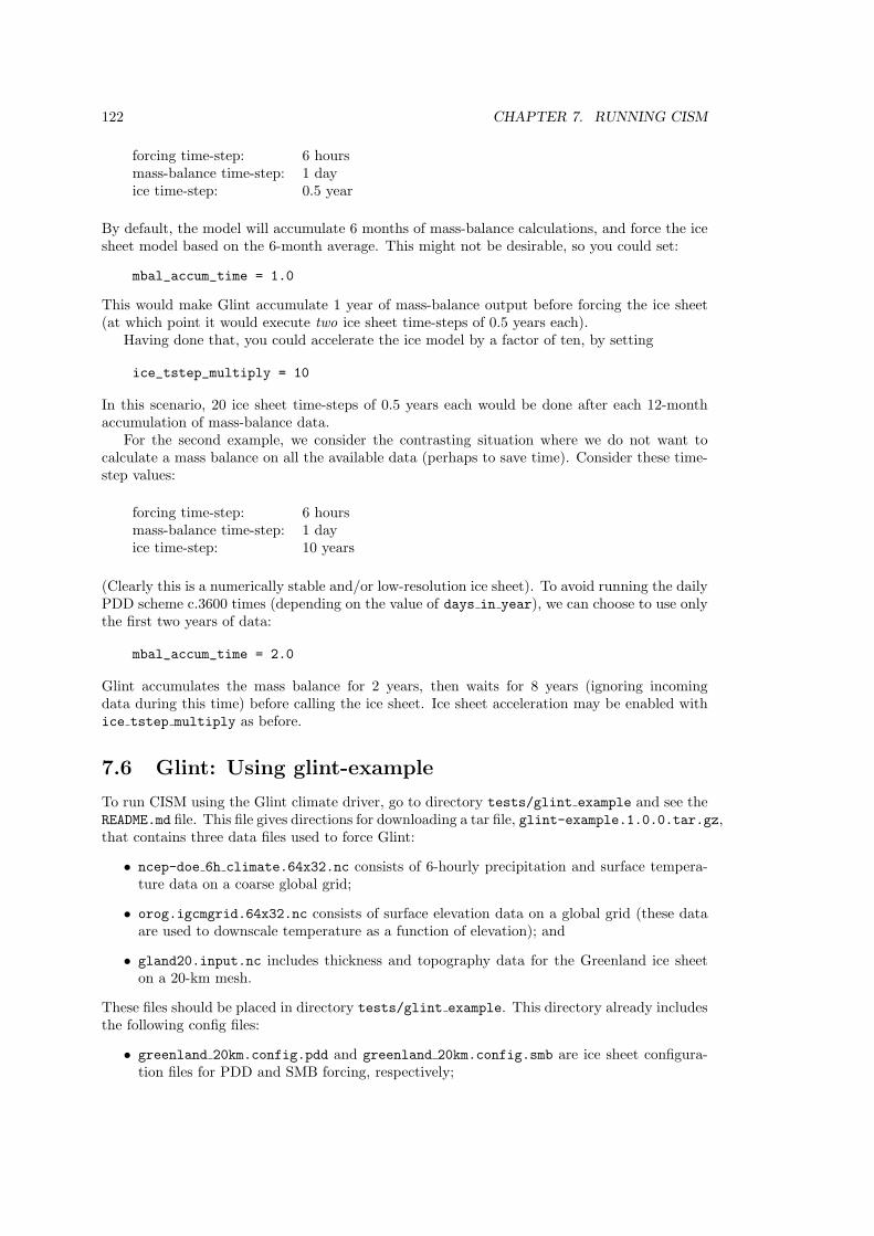
122 CHAPTER 7. RUNNING CISM
forcing time-step: 6 hoursmass-balance time-step: 1 dayice time-step: 0.5 year
By default, the model will accumulate 6 months of mass-balance calculations, and force the icesheet model based on the 6-month average. This might not be desirable, so you could set:
mbal_accum_time = 1.0
This would make Glint accumulate 1 year of mass-balance output before forcing the ice sheet(at which point it would execute two ice sheet time-steps of 0.5 years each).
Having done that, you could accelerate the ice model by a factor of ten, by setting
ice_tstep_multiply = 10
In this scenario, 20 ice sheet time-steps of 0.5 years each would be done after each 12-monthaccumulation of mass-balance data.
For the second example, we consider the contrasting situation where we do not want tocalculate a mass balance on all the available data (perhaps to save time). Consider these time-step values:
forcing time-step: 6 hoursmass-balance time-step: 1 dayice time-step: 10 years
(Clearly this is a numerically stable and/or low-resolution ice sheet). To avoid running the dailyPDD scheme c.3600 times (depending on the value of days in year), we can choose to use onlythe first two years of data:
mbal_accum_time = 2.0
Glint accumulates the mass balance for 2 years, then waits for 8 years (ignoring incomingdata during this time) before calling the ice sheet. Ice sheet acceleration may be enabled withice tstep multiply as before.
7.6 Glint: Using glint-example
To run CISM using the Glint climate driver, go to directory tests/glint example and see theREADME.md file. This file gives directions for downloading a tar file, glint-example.1.0.0.tar.gz,that contains three data files used to force Glint:
• ncep-doe 6h climate.64x32.nc consists of 6-hourly precipitation and surface tempera-ture data on a coarse global grid;
• orog.igcmgrid.64x32.nc consists of surface elevation data on a global grid (these dataare used to downscale temperature as a function of elevation); and
• gland20.input.nc includes thickness and topography data for the Greenland ice sheeton a 20-km mesh.
These files should be placed in directory tests/glint example. This directory already includesthe following config files:
• greenland 20km.config.pdd and greenland 20km.config.smb are ice sheet configura-tion files for PDD and SMB forcing, respectively;
7.7. SUPPLIED MASS-BALANCE SCHEMES 123
• glint example.config.pdd and glint example.config.smb are the corresponding cli-mate configuration files.
To apply the PDD scheme, type
./cism_driver greenland_20km.config.pdd glint-example.config.pdd
and to apply the SMB scheme, type
./cism_driver greenland_20km.config.smb glint-example.config.smb
The 6-hourly temperature and precipitation data are tailored for a PDD scheme. The same data,however, can also supply a crude surface mass balance and surface temperature in multipleelevation classes, imitating the forcing from a climate model such as CESM. (Accumulationis set equal to precipitation, and ablation is assumed to be linearly related to the downscaledtemperature. This scheme is convenient for testing but obviously is not appropriate for science.)By default, two files are output at a specified frequency: a history file containing variables ofinterest (e.g., thickness, velocity, and SMB) is output every 10 years, and a “hot” file containingthe variables required for exact restart is output every 1000 years.
7.7 Supplied mass-balance schemes
Users are free to supply their own mass-balance model for use with Glide. However, Glintincludes two positive-degree-day models for mass balance, one annual and one daily. Thissection describes how to configure and call these models.
NOTE: CISM2 development has focused on CESM-style coupling where the SMB is com-puted externally. The two PDD schemes (and the following description) are identical to thosein the original Glimmer code, but the schemes have not been extensively tested. Users shouldproceed with caution.
7.7.1 Annual PDD scheme
The annual PDD scheme is contained in the f90 module glimmer pdd, and the model parametersare contained in the derived type glimmer pdd params. Configuration data is contained in astandard CISM config file, which needs to be read before initializing the mass-balance model.The model is initialized by calling the subroutine glimmer pdd init, and the mass-balance maybe calculated annually by calling glimmer pdd mbal.
Example of use:
use glimmer_pdd
use glimmer_config
...
type(glimmer_pdd_params) :: pdd_scheme
type(ConfigSection),pointer :: config
...
call glimmer_pdd_init(pdd_scheme,config)
...
call glimmer_pdd_mbal(pdd_scheme,artm,arng,prcp,ablt,acab)
124 CHAPTER 7. RUNNING CISM
In the subroutine call to glimmer pdd mbal, apart from the parameter variable pdd scheme,there are three input fields (artm, arng and prcp), which are, respectively, the annual meanair temperature, annual temperature half-range, and annual accumulated precipitation fields.The final two arguments are output fields — annual ablation (ablt) and annual mass-balance(acab). Temperatures are in degrees Celsius, and precipitation, ablation and mass-balance aremeasured in m of water equivalent.
Degree-day calculation
The greater part of the information in the glimmer pdd params derived type comprises a look-uptable (the PDD table). The model is implemented this way for computational efficiency.
The table has two dimensions: mean annual air temperature (Ta) (as the second index) andannual air temperature half range (i.e., from July’s mean to the annual mean ∆Ta) (as the firstindex). Following Huybrechts and others [1991], daily air temperatures (T ′
a) are assumed tofollow a sinusoidal cycle
T ′a = Ta +∆Ta cos
(2πt
A
)+R(0, σ) (7.1)
where A is the period of a year and R is a random fluctuation drawn from a normal distributionwith mean 0 C and standard deviation σ C. Huybrechts and others [1991] indicate that thenumber of positive degree days (D, C days) for this temperature series can be evaluated as
D =1
σ√2π
A∫0
T ′a+2.5σ∫0
Ta × exp
(−(Ta − T ′
a)2
2σ2
)dTdt (7.2)
where t is time. The table is completed by evaluating this integral using a public-domainalgorithm (Romberg integration) by Bauer [1961]. The inner and outer integrals are coded astwo subroutines (inner integral and pdd integrand), which call the Romburg integrationrecursively.
The main parameter needed is the assumed standard deviation of daily air temperatures,which can be set in the configuration file (the default is 5 C).
The positive-degree days are then looked up in the table (as a function of Ta and ∆Ta). Wetake care to check that this look up is in done within the bounds of the table. The final valueof P is determined using bilinear interpolation given the four nearest entries in the table to theactual values of Ta and ∆Ta.
The remainder of the loop completes the calculation of the ablation and accumulation giventhis value for P .
Mass balance calculation
We use the following symbols: a is total annual ablation; as is potential snow ablation; b0 is thecapacity of the snowpack to hold meltwater by refreezing; the total number of positive degreedays (D); degree-day factors for snow and ice (fs and fi); and the fraction of snowfall thatcan be held in the snowpack as refrozen meltwater (Wmax). The degree-day factors have beenconverted from ice to water equivalents using the ratio of densities.
First, determine the depth of superimposed ice (b0) that would have to be formed beforerunoff (mass loss) occurs as a constant fraction (Wmax) of precipitation (P ):
b0 = WmaxP. (7.3)
Now determine the amount of snow melt by applying a constant degree-day factor for snow tothe number of positive degree-days:
as = fsD. (7.4)
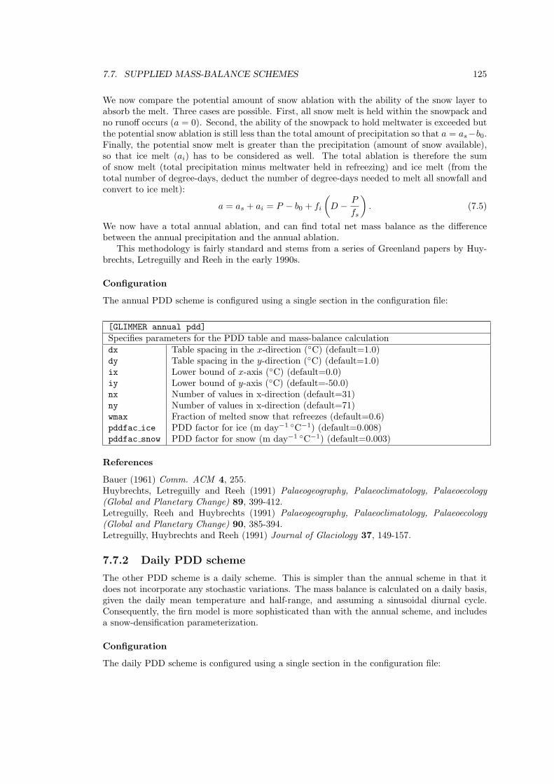
7.7. SUPPLIED MASS-BALANCE SCHEMES 125
We now compare the potential amount of snow ablation with the ability of the snow layer toabsorb the melt. Three cases are possible. First, all snow melt is held within the snowpack andno runoff occurs (a = 0). Second, the ability of the snowpack to hold meltwater is exceeded butthe potential snow ablation is still less than the total amount of precipitation so that a = as−b0.Finally, the potential snow melt is greater than the precipitation (amount of snow available),so that ice melt (ai) has to be considered as well. The total ablation is therefore the sumof snow melt (total precipitation minus meltwater held in refreezing) and ice melt (from thetotal number of degree-days, deduct the number of degree-days needed to melt all snowfall andconvert to ice melt):
a = as + ai = P − b0 + fi
(D − P
fs
). (7.5)
We now have a total annual ablation, and can find total net mass balance as the differencebetween the annual precipitation and the annual ablation.
This methodology is fairly standard and stems from a series of Greenland papers by Huy-brechts, Letreguilly and Reeh in the early 1990s.
Configuration
The annual PDD scheme is configured using a single section in the configuration file:
[GLIMMER annual pdd]
Specifies parameters for the PDD table and mass-balance calculationdx Table spacing in the x-direction (C) (default=1.0)dy Table spacing in the y-direction (C) (default=1.0)ix Lower bound of x-axis (C) (default=0.0)iy Lower bound of y-axis (C) (default=-50.0)nx Number of values in x-direction (default=31)ny Number of values in x-direction (default=71)wmax Fraction of melted snow that refreezes (default=0.6)pddfac ice PDD factor for ice (m day−1 C−1) (default=0.008)pddfac snow PDD factor for snow (m day−1 C−1) (default=0.003)
References
Bauer (1961) Comm. ACM 4, 255.Huybrechts, Letreguilly and Reeh (1991) Palaeogeography, Palaeoclimatology, Palaeoecology(Global and Planetary Change) 89, 399-412.Letreguilly, Reeh and Huybrechts (1991) Palaeogeography, Palaeoclimatology, Palaeoecology(Global and Planetary Change) 90, 385-394.Letreguilly, Huybrechts and Reeh (1991) Journal of Glaciology 37, 149-157.
7.7.2 Daily PDD scheme
The other PDD scheme is a daily scheme. This is simpler than the annual scheme in that itdoes not incorporate any stochastic variations. The mass balance is calculated on a daily basis,given the daily mean temperature and half-range, and assuming a sinusoidal diurnal cycle.Consequently, the firn model is more sophisticated than with the annual scheme, and includesa snow-densification parameterization.
Configuration
The daily PDD scheme is configured using a single section in the configuration file:
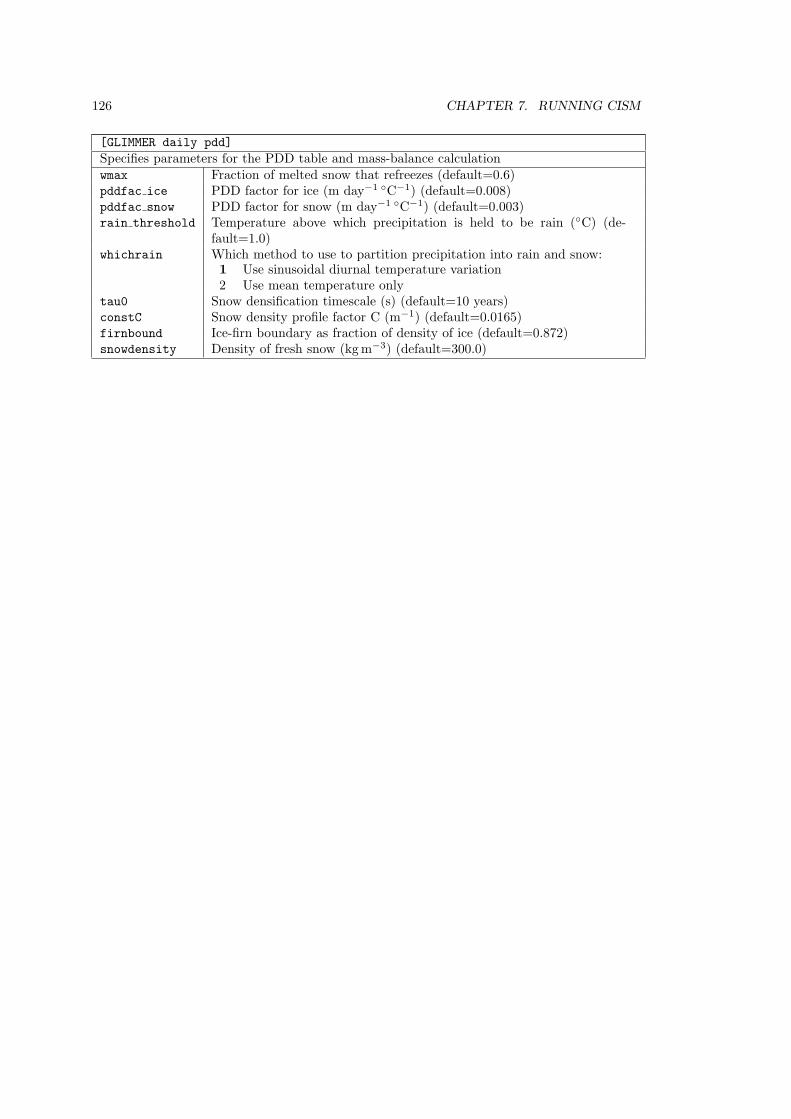
126 CHAPTER 7. RUNNING CISM
[GLIMMER daily pdd]
Specifies parameters for the PDD table and mass-balance calculationwmax Fraction of melted snow that refreezes (default=0.6)pddfac ice PDD factor for ice (m day−1 C−1) (default=0.008)pddfac snow PDD factor for snow (m day−1 C−1) (default=0.003)rain threshold Temperature above which precipitation is held to be rain (C) (de-
fault=1.0)whichrain Which method to use to partition precipitation into rain and snow:
1 Use sinusoidal diurnal temperature variation2 Use mean temperature only
tau0 Snow densification timescale (s) (default=10 years)constC Snow density profile factor C (m−1) (default=0.0165)firnbound Ice-firn boundary as fraction of density of ice (default=0.872)snowdensity Density of fresh snow (kgm−3) (default=300.0)
Chapter 8
Test Cases
Test cases for CISM include experiments with analytic solutions, standardized experiments with-out analytic solutions but for which community benchmarks are available, and some experimentsspecific to CISM which have been well characterized by CISM developers.
Here we organize test cases based on the velocity solver that is most appropriate for eachtest. Any velocity solver can be used with any test if the .config file settings are adjustedmanually. In some cases, however, the results may be difficult to interpret.
Each test directory includes a README.md file with some technical details about how torun the test. Many tests have python scripts that are used to set up the initial condition and,in some cases, execute the model. Some tests have an additional python script for analyzingthe CISM output.
The user must manually provide each test with access to the CISM executable. There areseveral ways to do this:
• Softlink the executable into the directory, e.g.:
ln -s ../../builds/mac-gnu/cism driver/cism driver ./
This is the recommended procedure during development so that the test will always beusing the most up-to-date version of the executable.
• Use the -e command line option to point to include an explicit path for the executable(for test case run scripts that support this option), e.g.:
./runDome.py -e ../../builds/mac-gnu/cism driver/cism driver
This is useful for quickly trying a different version of CISM (e.g., comparing serial andparallel executables).
• Add the directory containing the CISM executable to your environment PATH.
• Copy the executable into the directory. This is typically not the most efficient approach,but may make sense in some situations.
The python scripts generally have useful command line options that control their execution.Typically, you can see details by using the --help (or -h) command line option, e.g.:
./runDome.py --help
The various tests are described below.
8.1 Shallow-Ice Test Cases
These tests are primarily useful for testing the shallow-ice approximation (SIA) dynamical core,Glide (see Chapter 4). The Glissade dycore also has a shallow-ice option (see Section 6.2.2).
127
128 CHAPTER 8. TEST CASES
8.1.1 Halfar dome
The Halfar test case describes the time evolution of a parabolic dome of ice, as described byHalfar (1983). For a flat-bedded SIA problem, this case has an analytic solution for the timevarying ice thickness. We start with the general SIA ice evolution equation,
∂H
∂t= ∇ · (ΓHn+2|∇H|n−1∇H), (8.1)
where n is the exponent in the Glen flow law, commonly taken as 3, and Γ is a positive constant:
Γ =2
n+ 2A(ρg)n. (8.2)
For n = 3, the time-dependent solution is
H(t, r) = H0
(t0t
) 19
1−(( t0t
) 118 r
R0
) 43
37
, (8.3)
where
t0 =1
18Γ
(7
4
)3R4
0
H70
, (8.4)
and H0, R0 are the central height of the dome and its radius at time t = t0. For more details,see Halfar (1983), Bueler et al. (2005), and this link1.
Provided files
Our implementation of the Halfar dome test has an initial radius of R0 = 21.2 km and an initialthickness of H = 707.1 m. These values can be changed by editing the halfarDome function inrunHalfar.py.
• README.mdInformation about the test case, including technical details about running it.
• halfar.configThis is the config file defining CISM options. It is set up to run Glide.
• halfar-HO.configThis alternative config file is set up to run Glissade using the Blatter-Pattyn approximationof Stokes flow. By manually setting which ho approx under [ho options], users canchoose other approximations (see Section 7.3).
• runHalfar.pyThis python script generates the dome initial condition and runs CISM.
• halfar results.pyThis script compares model results to the analytic solution.
1http://www.giseis.alaska.edu/input/carl/teaching/extra/bueler notes.pdf
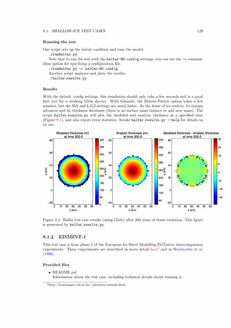
8.1. SHALLOW-ICE TEST CASES 129
Running the test
One script sets up the initial condition and runs the model:./runHalfar.py
Note that to run the test with the halfar-HO.config settings, you can use the -c comman-dline option for specifying a configuration file:
./runHalfar.py -c halfar-HO.config
Another script analyzes and plots the results:./halfar results.py
Results
With the default .config settings, this simulation should only take a few seconds and is a goodfirst test for a working Glide dycore. With Glissade, the Blatter-Pattyn option takes a fewminutes, but the SIA and L1L2 settings are much faster. As the dome of ice evolves, its marginadvances and its thickness decreases (there is no surface mass balance to add new mass). Thescript halfar results.py will plot the modeled and analytic thickness at a specified time(Figure 8.1), and also report error statistics. Invoke halfar results.py --help for details onits use.
Figure 8.1: Halfar test case results (using Glide) after 200 years of dome evolution. This figureis generated by halfar results.py.
8.1.2 EISMINT-1
This test case is from phase 1 of the European Ice Sheet Modelling INiTiative intercomparisonexperiments. These experiments are described in more detail here2 and in Huybrechts et al.(1996).
Provided files
• README.mdInformation about the test case, including technical details about running it.
2http://homepages.vub.ac.be/˜phuybrec/eismint.html
130 CHAPTER 8. TEST CASES
• *.configThere are .config files for each of the six experiments in EISMINT 1: three fixed marginexperiments (fm) and three moving margin experiments (mm).
Running the test
There is no script for running these experiments. They are simply run manually, e.g. using:./cism driver e1-fm.1.config
Results
These experiments are meant to be run to steady-state, and the supplied .config files are setup to run for long enough to do this. These simulations take more than a few minutes tocomplete. As the ice sheet evolves, its shape eventually equilibrates with the imposed surfacemass balance. Currently there is no script for analyzing the model results. However, users canvisually compare their results to those in Huybrechts et al. (1996).
8.1.3 EISMINT-2
This test case is from phase 2 of the European Ice Sheet Modelling INiTiative intercomparisonexperiments. These experiments are described in more detail here3 and in Payne et al. (2000).
Provided files
• README.mdInformation about the test case, including technical details about running it.
• *.configThere are 11 .config files: one for each of the experiments described in Payne et al. (2000).
• mound.nc, trough.ncThese are input netCDF files used by the EISMINT-2 experiments.
Running the test
There is no script for running these experiments. They are run manually, e.g. using:./cism driver e2.a.config
Results
These experiments are meant to be run to steady-state, and the supplied .config files are set upto run for long enough to do this. Some experiments use the final state of a previous experimentas the initial condition (e.g., most experiments following experiment A use the final state fromA as an initial condition). See the experimental descriptions in Payne et al. (2000) for details.These simulations take more than a few minutes to complete. As the ice sheet evolves, its shapeequilibrates with the imposed surface mass balance. There is no script for analyzing modelresults, but users can visually compare their results to those in Payne et al. (2000), and alsocompare model diagnostics (e.g., ice area, volume, and maximum thickness) to Table 4 of thatpaper.
8.1.4 Glint example
Section 7.6 explains how to set up and run the Glint example test case. We summarize thatinformation here.
3http://homepages.vub.ac.be/˜phuybrec/eismint.html
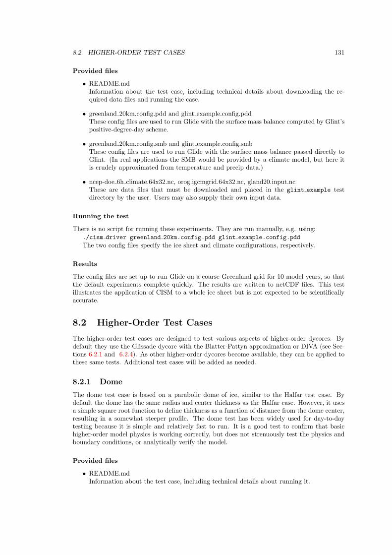
8.2. HIGHER-ORDER TEST CASES 131
Provided files
• README.mdInformation about the test case, including technical details about downloading the re-quired data files and running the case.
• greenland 20km.config.pdd and glint example.config.pddThese config files are used to run Glide with the surface mass balance computed by Glint’spositive-degree-day scheme.
• greenland 20km.config.smb and glint example.config.smbThese config files are used to run Glide with the surface mass balance passed directly toGlint. (In real applications the SMB would be provided by a climate model, but here itis crudely approximated from temperature and precip data.)
• ncep-doe 6h climate.64x32.nc, orog.igcmgrid.64x32.nc, gland20.input.ncThese are data files that must be downloaded and placed in the glint example testdirectory by the user. Users may also supply their own input data.
Running the test
There is no script for running these experiments. They are run manually, e.g. using:./cism driver greenland 20km.config.pdd glint example.config.pdd
The two config files specify the ice sheet and climate configurations, respectively.
Results
The config files are set up to run Glide on a coarse Greenland grid for 10 model years, so thatthe default experiments complete quickly. The results are written to netCDF files. This testillustrates the application of CISM to a whole ice sheet but is not expected to be scientificallyaccurate.
8.2 Higher-Order Test Cases
The higher-order test cases are designed to test various aspects of higher-order dycores. Bydefault they use the Glissade dycore with the Blatter-Pattyn approximation or DIVA (see Sec-tions 6.2.1 and 6.2.4). As other higher-order dycores become available, they can be applied tothese same tests. Additional test cases will be added as needed.
8.2.1 Dome
The dome test case is based on a parabolic dome of ice, similar to the Halfar test case. Bydefault the dome has the same radius and center thickness as the Halfar case. However, it usesa simple square root function to define thickness as a function of distance from the dome center,resulting in a somewhat steeper profile. The dome test has been widely used for day-to-daytesting because it is simple and relatively fast to run. It is a good test to confirm that basichigher-order model physics is working correctly, but does not strenuously test the physics andboundary conditions, or analytically verify the model.
Provided files
• README.mdInformation about the test case, including technical details about running it.
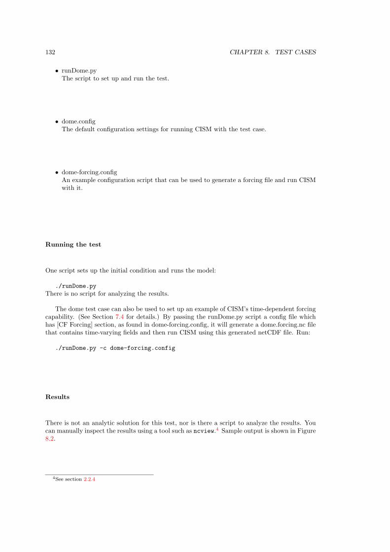
132 CHAPTER 8. TEST CASES
• runDome.pyThe script to set up and run the test.
• dome.configThe default configuration settings for running CISM with the test case.
• dome-forcing.configAn example configuration script that can be used to generate a forcing file and run CISMwith it.
Running the test
One script sets up the initial condition and runs the model:
./runDome.py
There is no script for analyzing the results.
The dome test case can also be used to set up an example of CISM’s time-dependent forcingcapability. (See Section 7.4 for details.) By passing the runDome.py script a config file whichhas [CF Forcing] section, as found in dome-forcing.config, it will generate a dome.forcing.nc filethat contains time-varying fields and then run CISM using this generated netCDF file. Run:
./runDome.py -c dome-forcing.config
Results
There is not an analytic solution for this test, nor is there a script to analyze the results. Youcan manually inspect the results using a tool such as ncview.4 Sample output is shown in Figure8.2.
4See section 2.2.4
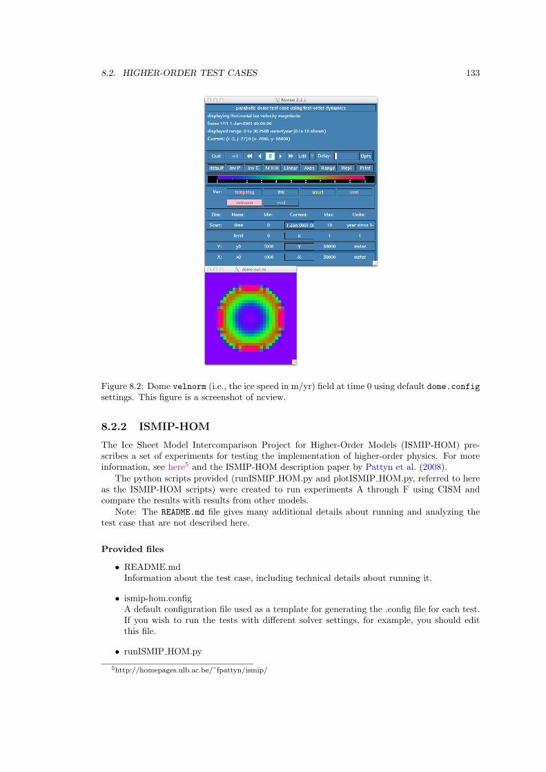
8.2. HIGHER-ORDER TEST CASES 133
Figure 8.2: Dome velnorm (i.e., the ice speed in m/yr) field at time 0 using default dome.configsettings. This figure is a screenshot of ncview.
8.2.2 ISMIP-HOM
The Ice Sheet Model Intercomparison Project for Higher-Order Models (ISMIP-HOM) pre-scribes a set of experiments for testing the implementation of higher-order physics. For moreinformation, see here5 and the ISMIP-HOM description paper by Pattyn et al. (2008).
The python scripts provided (runISMIP HOM.py and plotISMIP HOM.py, referred to hereas the ISMIP-HOM scripts) were created to run experiments A through F using CISM andcompare the results with results from other models.
Note: The README.md file gives many additional details about running and analyzing thetest case that are not described here.
Provided files
• README.mdInformation about the test case, including technical details about running it.
• ismip-hom.configA default configuration file used as a template for generating the .config file for each test.If you wish to run the tests with different solver settings, for example, you should editthis file.
• runISMIP HOM.py
5http://homepages.ulb.ac.be/˜fpattyn/ismip/
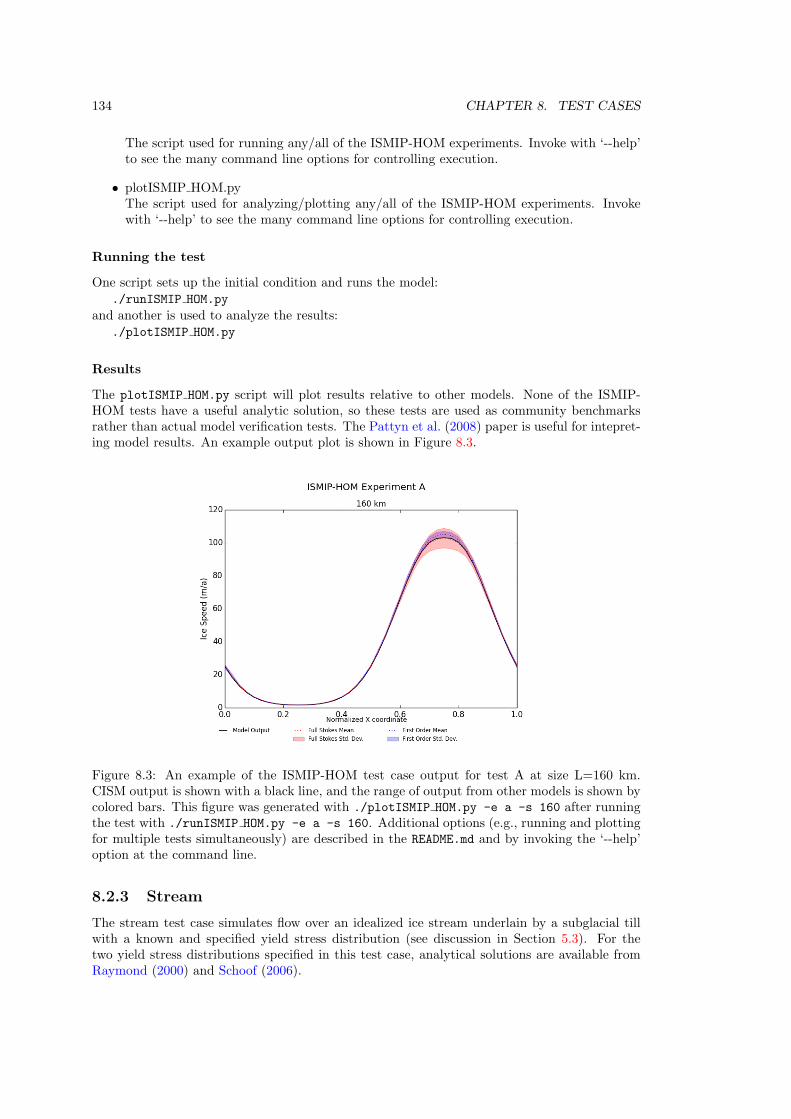
134 CHAPTER 8. TEST CASES
The script used for running any/all of the ISMIP-HOM experiments. Invoke with ‘--help’to see the many command line options for controlling execution.
• plotISMIP HOM.pyThe script used for analyzing/plotting any/all of the ISMIP-HOM experiments. Invokewith ‘--help’ to see the many command line options for controlling execution.
Running the test
One script sets up the initial condition and runs the model:./runISMIP HOM.py
and another is used to analyze the results:./plotISMIP HOM.py
Results
The plotISMIP HOM.py script will plot results relative to other models. None of the ISMIP-HOM tests have a useful analytic solution, so these tests are used as community benchmarksrather than actual model verification tests. The Pattyn et al. (2008) paper is useful for intepret-ing model results. An example output plot is shown in Figure 8.3.
Figure 8.3: An example of the ISMIP-HOM test case output for test A at size L=160 km.CISM output is shown with a black line, and the range of output from other models is shown bycolored bars. This figure was generated with ./plotISMIP HOM.py -e a -s 160 after runningthe test with ./runISMIP HOM.py -e a -s 160. Additional options (e.g., running and plottingfor multiple tests simultaneously) are described in the README.md and by invoking the ‘--help’option at the command line.
8.2.3 Stream
The stream test case simulates flow over an idealized ice stream underlain by a subglacial tillwith a known and specified yield stress distribution (see discussion in Section 5.3). For thetwo yield stress distributions specified in this test case, analytical solutions are available fromRaymond (2000) and Schoof (2006).
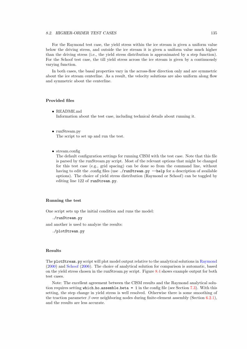
8.2. HIGHER-ORDER TEST CASES 135
For the Raymond test case, the yield stress within the ice stream is given a uniform valuebelow the driving stress, and outside the ice stream it is given a uniform value much higherthan the driving stress (i.e., the yield stress distribution is approximated by a step function).For the Schoof test case, the till yield stress across the ice stream is given by a continuouslyvarying function.
In both cases, the basal properties vary in the across-flow direction only and are symmetricabout the ice stream centerline. As a result, the velocity solutions are also uniform along flowand symmetric about the centerline.
Provided files
• README.mdInformation about the test case, including technical details about running it.
• runStream.pyThe script to set up and run the test.
• stream.configThe default configuration settings for running CISM with the test case. Note that this fileis parsed by the runStream.py script. Most of the relevant options that might be changedfor this test case (e.g., grid spacing) can be done so from the command line, withouthaving to edit the .config files (use ./runStream.py --help for a description of availableoptions). The choice of yield stress distribution (Raymond or Schoof) can be toggled byediting line 122 of runStream.py.
Running the test
One script sets up the initial condition and runs the model:
./runStream.py
and another is used to analyze the results:
./plotStream.py
Results
The plotStream.py script will plot model output relative to the analytical solutions in Raymond(2000) and Schoof (2006). The choice of analytical solution for comparison is automatic, basedon the yield stress chosen in the runStream.py script. Figure 8.4 shows example output for bothtest cases.
Note: The excellent agreement between the CISM results and the Raymond analytical solu-tion requires setting which ho assemble beta = 1 in the config file (see Section 7.3). With thissetting, the step change in yield stress is well resolved. Otherwise there is some smoothing ofthe traction parameter β over neighboring nodes during finite-element assembly (Section 6.2.1),and the results are less accurate.
136 CHAPTER 8. TEST CASES
Figure 8.4: Comparison between CISM model output (black) and analytic solution (red) forthe Raymond (top) and Schoof (bottom) stream test cases. This figure was generated with./plotStream.py after running the test with ./runStream.py. Additional runtime options aredescribed in the README.md and by invoking the ‘--help’ option at the command line.
8.2.4 Confined shelf
The confined shelf test is based on tests 3 and 4 of the idealized (i.e., not Ross) EISMINTshelf test cases. It simulates the flow within an idealized, 500 m thick ice shelf in a confined,rectangular embayment. Grounded ice is not explicitly modeled but included in the modelsetup as Dirichlet boundary conditions for velocity along the ice shelf edges. More detailed
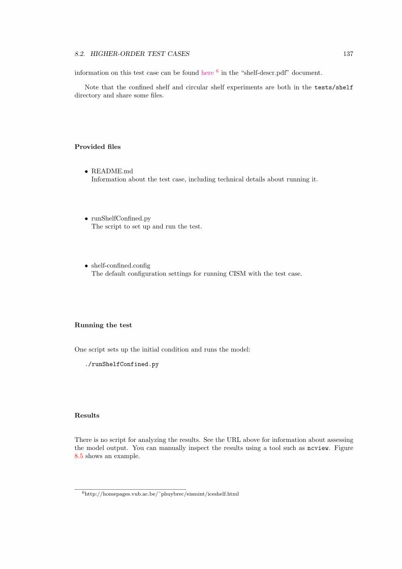
8.2. HIGHER-ORDER TEST CASES 137
information on this test case can be found here 6 in the “shelf-descr.pdf” document.
Note that the confined shelf and circular shelf experiments are both in the tests/shelf
directory and share some files.
Provided files
• README.mdInformation about the test case, including technical details about running it.
• runShelfConfined.pyThe script to set up and run the test.
• shelf-confined.configThe default configuration settings for running CISM with the test case.
Running the test
One script sets up the initial condition and runs the model:
./runShelfConfined.py
Results
There is no script for analyzing the results. See the URL above for information about assessingthe model output. You can manually inspect the results using a tool such as ncview. Figure8.5 shows an example.
6http://homepages.vub.ac.be/˜phuybrec/eismint/iceshelf.html
138 CHAPTER 8. TEST CASES
Figure 8.5: Confined shelf velnorm field using default shelf-confined.config settings. Thisfigure is a screenshot of ncview.
8.2.5 Circular shelf
The circular shelf test case is a variant on the confined shelf discussed above. It simulates theflow within a circular ice shelf with a uniform thickness of 1000 m, which is grounded at a singlegrid point at its center. This test case confirms a working “floating ice” boundary condition in2D (i.e., in map plane view) and also confirms radial symmetry.
Note that the confined shelf and circular shelf experiments are both in the tests/shelf
directory and share some files.
Provided files
• README.mdInformation about the test case, including technical details about running it.
• runShelfCircular.pyThe script to set up and run the test.
• shelf-circular.configThe default configuration settings for running CISM with the test case.
Running the test
One script sets up the initial condition and runs the model:
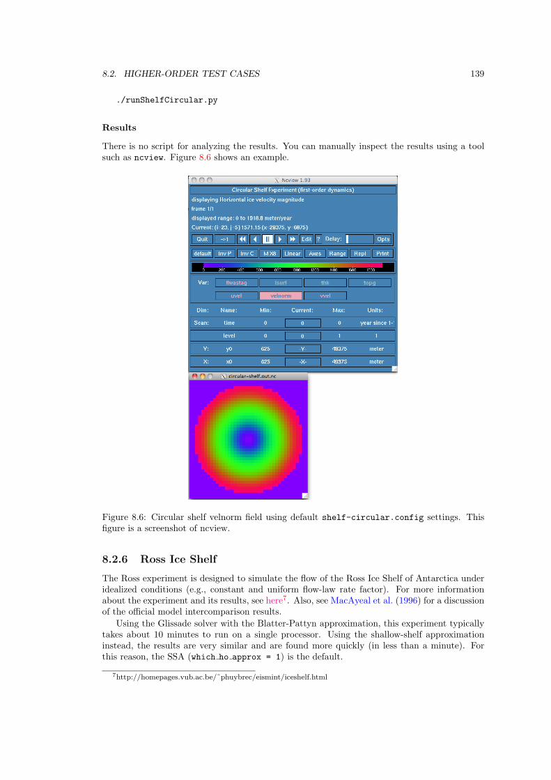
8.2. HIGHER-ORDER TEST CASES 139
./runShelfCircular.py
Results
There is no script for analyzing the results. You can manually inspect the results using a toolsuch as ncview. Figure 8.6 shows an example.
Figure 8.6: Circular shelf velnorm field using default shelf-circular.config settings. Thisfigure is a screenshot of ncview.
8.2.6 Ross Ice Shelf
The Ross experiment is designed to simulate the flow of the Ross Ice Shelf of Antarctica underidealized conditions (e.g., constant and uniform flow-law rate factor). For more informationabout the experiment and its results, see here7. Also, see MacAyeal et al. (1996) for a discussionof the official model intercomparison results.
Using the Glissade solver with the Blatter-Pattyn approximation, this experiment typicallytakes about 10 minutes to run on a single processor. Using the shallow-shelf approximationinstead, the results are very similar and are found more quickly (in less than a minute). Forthis reason, the SSA (which ho approx = 1) is the default.
7http://homepages.vub.ac.be/˜phuybrec/eismint/iceshelf.html
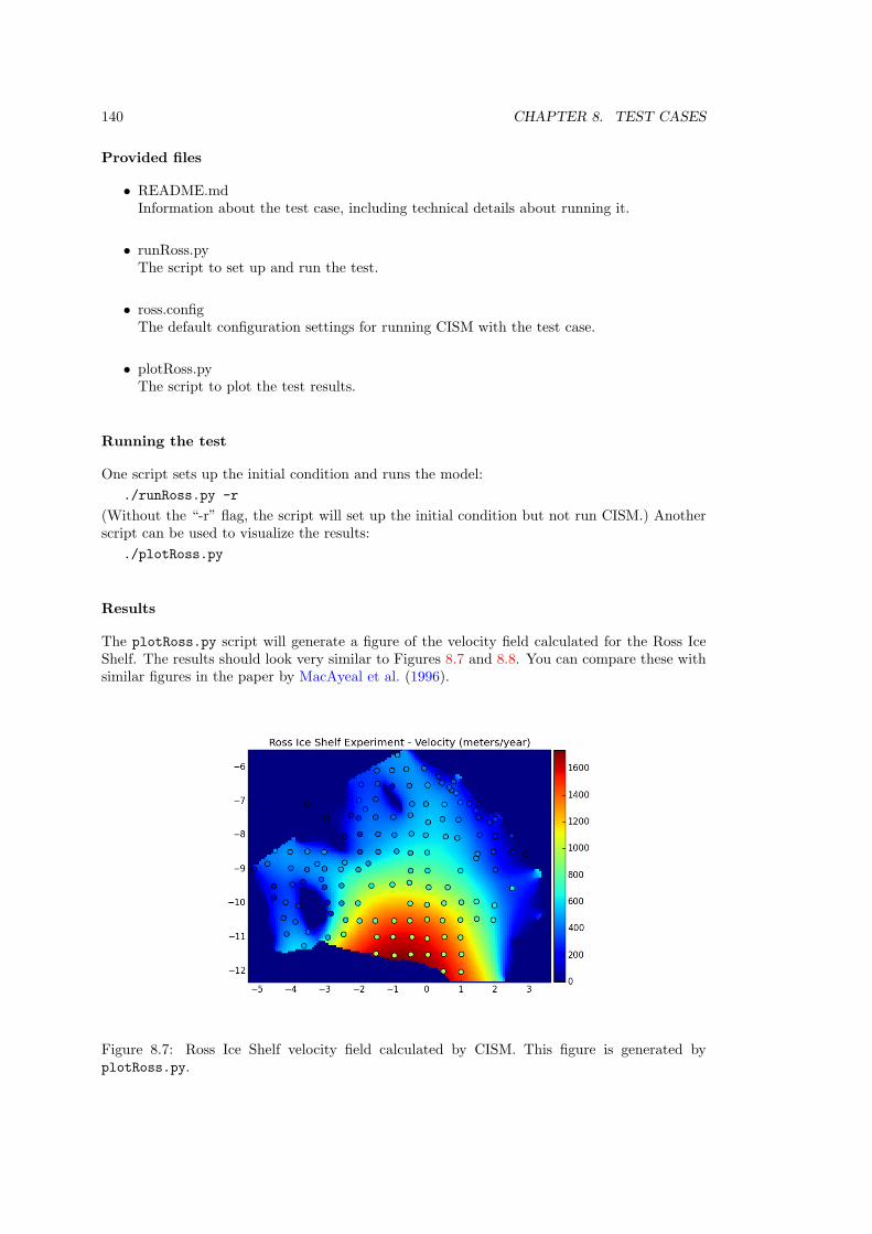
140 CHAPTER 8. TEST CASES
Provided files
• README.mdInformation about the test case, including technical details about running it.
• runRoss.pyThe script to set up and run the test.
• ross.configThe default configuration settings for running CISM with the test case.
• plotRoss.pyThe script to plot the test results.
Running the test
One script sets up the initial condition and runs the model:
./runRoss.py -r
(Without the “-r” flag, the script will set up the initial condition but not run CISM.) Anotherscript can be used to visualize the results:
./plotRoss.py
Results
The plotRoss.py script will generate a figure of the velocity field calculated for the Ross IceShelf. The results should look very similar to Figures 8.7 and 8.8. You can compare these withsimilar figures in the paper by MacAyeal et al. (1996).
Figure 8.7: Ross Ice Shelf velocity field calculated by CISM. This figure is generated byplotRoss.py.
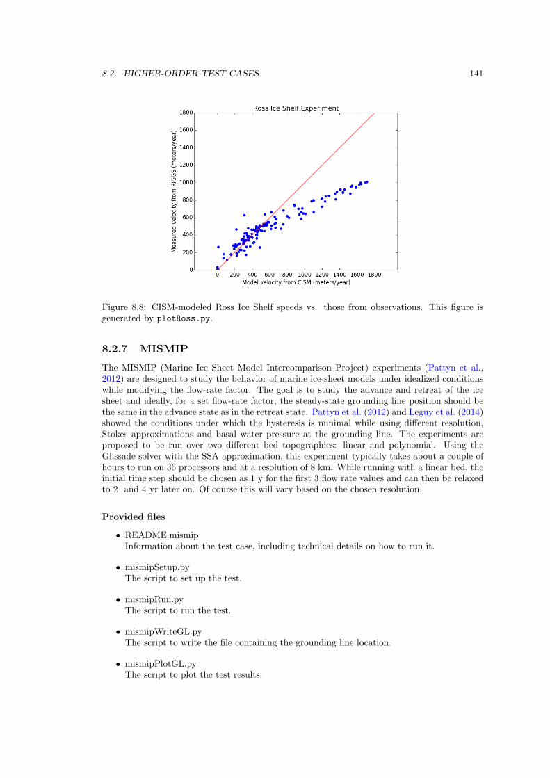
8.2. HIGHER-ORDER TEST CASES 141
Figure 8.8: CISM-modeled Ross Ice Shelf speeds vs. those from observations. This figure isgenerated by plotRoss.py.
8.2.7 MISMIP
The MISMIP (Marine Ice Sheet Model Intercomparison Project) experiments (Pattyn et al.,2012) are designed to study the behavior of marine ice-sheet models under idealized conditionswhile modifying the flow-rate factor. The goal is to study the advance and retreat of the icesheet and ideally, for a set flow-rate factor, the steady-state grounding line position should bethe same in the advance state as in the retreat state. Pattyn et al. (2012) and Leguy et al. (2014)showed the conditions under which the hysteresis is minimal while using different resolution,Stokes approximations and basal water pressure at the grounding line. The experiments areproposed to be run over two different bed topographies: linear and polynomial. Using theGlissade solver with the SSA approximation, this experiment typically takes about a couple ofhours to run on 36 processors and at a resolution of 8 km. While running with a linear bed, theinitial time step should be chosen as 1 y for the first 3 flow rate values and can then be relaxedto 2 and 4 yr later on. Of course this will vary based on the chosen resolution.
Provided files
• README.mismipInformation about the test case, including technical details on how to run it.
• mismipSetup.pyThe script to set up the test.
• mismipRun.pyThe script to run the test.
• mismipWriteGL.pyThe script to write the file containing the grounding line location.
• mismipPlotGL.pyThe script to plot the test results.
142 CHAPTER 8. TEST CASES
• mismip.config.templateThe default configuration template settings for running CISM with the test case. Inputswill vary based on the options used with the setup file.
• runCISM.cheyenne.templateThe template script to submit a job on Cheyenne HPC system. The wall time, number ofnodes and processors will need to be adjusted depending on the need of the simulation.
Running the test
For detailed instruction, follow the instruction from the README.mismip file. In short the orderof operations are:
Set up the experiment (add options if need be):
> python mismipSetup.py
Run the experiment (add options if need be):
> python mismipRun.py
Write the grounding line position to a file (add options if need be):
> python mismipWriteGL.py
Plot the results (add options if need be):
> python mismipPlotGL.py
Results
The mismipPlotGL.py script will generate a figure of the grounding line position as a functionof the flow-rate factor inverse at the end of each experiment and the semi-analytic solution fromSchoof (2007). The results should look very similar to Figures 8.9 (for the linear bed) and 8.10(for the polynomial bed) when using the ”powerlaw” (Schoof, 2007) basal friction law. You cancompare these with similar figures in the papers by Pattyn et al. (2012) and Leguy et al. (2014).
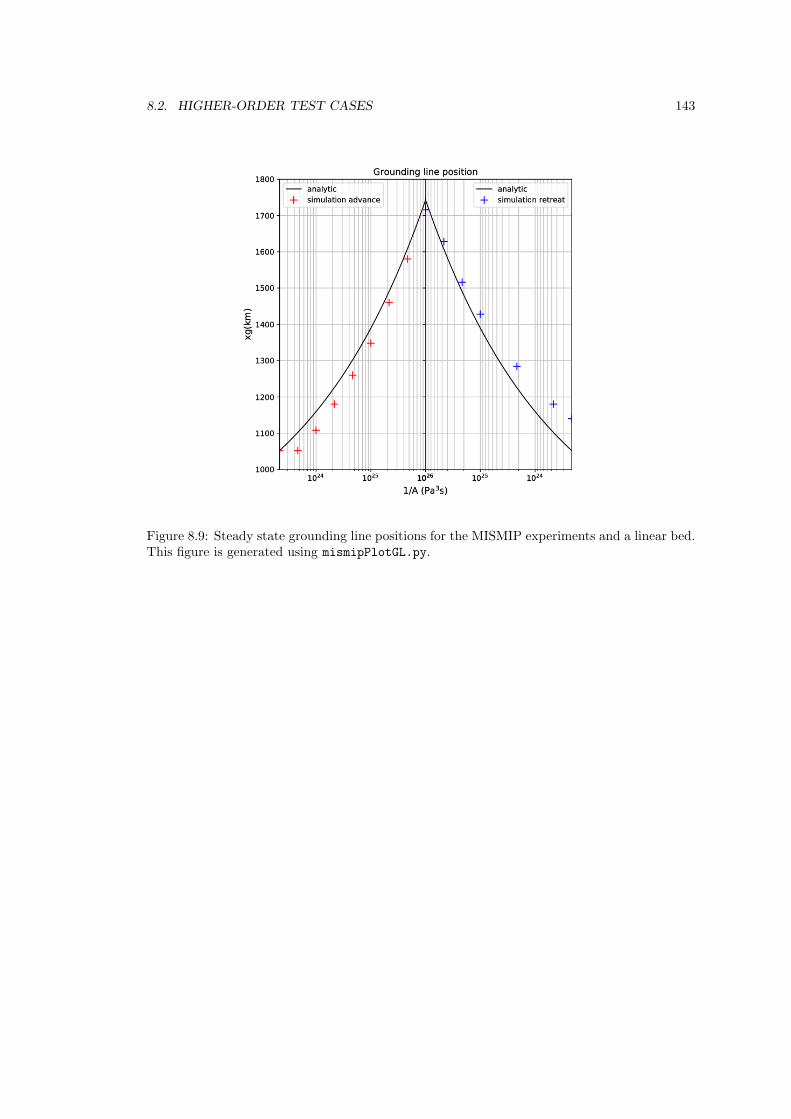
8.2. HIGHER-ORDER TEST CASES 143
Figure 8.9: Steady state grounding line positions for the MISMIP experiments and a linear bed.This figure is generated using mismipPlotGL.py.
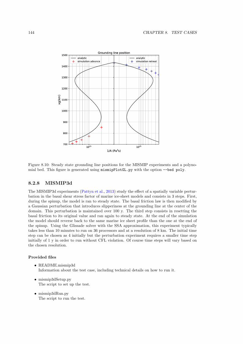
144 CHAPTER 8. TEST CASES
Figure 8.10: Steady state grounding line positions for the MISMIP experiments and a polyno-mial bed. This figure is generated using mismipPlotGL.py with the option --bed poly.
8.2.8 MISMIP3d
The MISMIP3d experiments (Pattyn et al., 2013) study the effect of a spatially variable pertur-bation in the basal shear stress factor of marine ice-sheet models and consists in 3 steps. First,during the spinup, the model is ran to steady state. The basal friction law is then modified bya Gaussian perturbation that introduces slipperiness at the grounding line at the center of thedomain. This perturbation is maintained over 100 y. The third step consists in resetting thebasal friction to its original value and ran again to steady state. At the end of the simulationthe model should reverse back to the same marine ice sheet profile than the one at the end ofthe spinup. Using the Glissade solver with the SSA approximation, this experiment typicallytakes less than 10 minutes to run on 36 processors and at a resolution of 8 km. The initial timestep can be chosen as 4 initially but the perturbation experiment requires a smaller time stepinitially of 1 y in order to run without CFL violation. Of course time steps will vary based onthe chosen resolution.
Provided files
• README.mismip3dInformation about the test case, including technical details on how to run it.
• mismip3dSetup.pyThe script to set up the test.
• mismip3dRun.pyThe script to run the test.
8.2. HIGHER-ORDER TEST CASES 145
• mismip3dWriteGL.pyThe script to write the file containing the grounding line location.
• mismip3dPlotGL.pyThe script to plot the test results.
• mismip3d.config.templateThe default configuration template settings for running CISM with the test case. Inputswill vary based on the options used with the setup file.
• runCISM.cheyenne.templateThe template script to submit a job on Cheyenne HPC system. The wall time, number ofnodes and processors will need to be adjusted depending on the need of the simulation.
Running the test
For detailed instruction, follow the instruction from the README.mismip3d file. In short theorder of operations are:
Set up the experiment (add options if need be):
> python mismip3dSetup.py
Run the experiment (add options if need be):
> python mismip3dRun.py
Write the grounding line position to a file (add options if need be):
> python mismip3dWriteGL.py
Plot the results:
> python mismip3dPlotGL.py
Results
The mismip3dPlotGL.py script will generate a figure of the grounding line positions for eachstep of the experiments as a function of spatial location. Note that the grounding line positionfor the non-perturbed experiment can be compared to the semi-analytic solution from Schoof(2007). The results should look very similar to Figure 8.11 when using the ”powerlaw” (Schoof,2007) basal friction law. You can compare these with similar figures in Pattyn et al. (2013) (inthe paper the results are plotted over half of the y-axis due to symmetry of the perturbation).
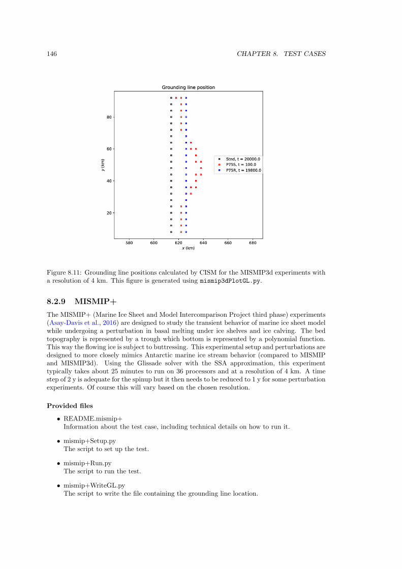
146 CHAPTER 8. TEST CASES
Figure 8.11: Grounding line positions calculated by CISM for the MISMIP3d experiments witha resolution of 4 km. This figure is generated using mismip3dPlotGL.py.
8.2.9 MISMIP+
The MISMIP+ (Marine Ice Sheet and Model Intercomparison Project third phase) experiments(Asay-Davis et al., 2016) are designed to study the transient behavior of marine ice sheet modelwhile undergoing a perturbation in basal melting under ice shelves and ice calving. The bedtopography is represented by a trough which bottom is represented by a polynomial function.This way the flowing ice is subject to buttressing. This experimental setup and perturbations aredesigned to more closely mimics Antarctic marine ice stream behavior (compared to MISMIPand MISMIP3d). Using the Glissade solver with the SSA approximation, this experimenttypically takes about 25 minutes to run on 36 processors and at a resolution of 4 km. A timestep of 2 y is adequate for the spinup but it then needs to be reduced to 1 y for some perturbationexperiments. Of course this will vary based on the chosen resolution.
Provided files
• README.mismip+Information about the test case, including technical details on how to run it.
• mismip+Setup.pyThe script to set up the test.
• mismip+Run.pyThe script to run the test.
• mismip+WriteGL.pyThe script to write the file containing the grounding line location.
8.2. HIGHER-ORDER TEST CASES 147
• mismip+PlotGL.pyThe script to plot the test results.
• mismip+.config.templateThe default configuration template settings for running CISM with the test case. Inputswill vary based on the options used with the setup file.
• runCISM.cheyenne.templateThe template script to submit a job on Cheyenne HPC system. The wall time, number ofnodes and processors will need to be adjusted depending on the need of the simulation.
Running the test
For detailed instruction, follow the instruction from the README.mismip+ file. In short the orderof operations are:
Set up the experiment (add options if need be):
> python mismip+Setup.py
Run the experiment (add options if need be):
> python mismip+Run.py
Write the grounding line position to a file (add options if need be):
> python mismip+WriteGL.py
Plot the results:
> python mismip+PlotGL.py
Results
The mismip+PlotGL.py script will generate a figure of the grounding line positions and thegrounded area for each step of the control and perturbed experiments as a function of spatiallocation and time respectively. The results should look very similar to Figure 8.12 when usingthe ”Schoof2005” (Schoof, 2005; Leguy et al., 2014) basal friction law. You can compare it withsimilar figures in Asay-Davis et al. (2016).
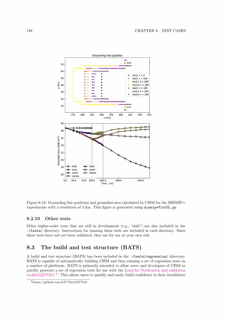
148 CHAPTER 8. TEST CASES
Figure 8.12: Grounding line positions and grounded area calculated by CISM for the MISMIP+experiments with a resolution of 4 km. This figure is generated using mismip+PlotGL.py.
8.2.10 Other tests
Other higher-order tests that are still in development (e.g., “slab”) are also included in the./tests/ directory. Instructions for running these tests are included in each directory. Sincethese tests have not yet been validated, they are for use at your own risk.
8.3 The build and test structure (BATS)
A build and test structure (BATS) has been included in the ./tests/regression/ directory.BATS is capable of automatically building CISM and then running a set of regression tests ona number of platforms. BATS is primarily intended to allow users and developers of CISM toquickly generate a set of regression tests for use with the Land Ice Verification and validationtoolkit(LIVVkit) 8. This allows users to quickly and easily build confidence in their installation
8https://github.com/LIVVkit/LIVVkit
8.3. THE BUILD AND TEST STRUCTURE (BATS) 149
of CISM and, by extension, their scientific results.
Provided files
• README.mdInformation about the build and test structure, including technical details about using it.
• build and test.py
The main script to build CISM, and run a set of regression tests.
• setup hopper.bash and setup titan.bash
Scripts to load the needed modules on the higher-performance-computing architecturesHopper (NERSC) and Titan (OLCF).
• util/
A directory containing a set of helper python modules and files for build and test.py.
Using BATS
BATS works very similar to how you would build CISM and run one or more CISM tests. BATSwill build a version of CISM, and then either run a set of regression tests if you are using apersonal computer (PC), or setup a series of regression tests and generate a job submissionscript if you are using a high-performance-computing architecture (HPC).
For example, on the HPC Titan, if you wanted to build CISM using the gnu compiler, andrun a set of regression tests, you would run these commands:
cd tests/regression/
source setup_titan.bash
./build_and_test.py -p titan -c gnu -b ./build
which will result in BATS generating all the CMake build files into a new directory calledbuild and building CISM into the directory build/cism driver. BATS will then setup a setof CISM’s higher-order tests:
• Dome (at a variety of resolutions and processor counts)
• Circular and confined shelf
• ISMIP-HOM a and c (at 20 and 80 km resolutions)
• ISMIP-HOM f
• Stream
All the files associated with each test will be output to a new directory called reg test/titan-gnu,which has a directory structure that mirrors CISMS test directory structure:
reg_test/
PLATFORM-COMPILER/
CMakeCache.txt
higher-order/
dome/
dome.RESO.pPRC.*
timing/
dome-t?.RESO.pPRC.*
ismip-hom
ismip-hom-a.RESO.pPRC.*
150 CHAPTER 8. TEST CASES
ismip-hom-c.RESO.pPRC.*
ismip-hom-f.0100.pPRC.*
shelf
shelf-circular.RESO.pPRC.*
shelf-confined.RESO.pPRC.*
stream
stream.RESO.pPRC.*
--------------------------------------------
Jobs/
platform_job.small
platform_job.small_timing_?
platform_job.large
platform_job.large_timing_?
submit_all_jobs.bash
clean_timing.bash
where * and ? are POSIX regular expressions metacharacters, RESO is a number indicating theresolution the test was run at (the meaning of the number is test dependent), and pPRC is anumber, prefixed by a p, indicating the number of processors used when running the model.This reg test directory will be formatted to used with LIVVkit directly. Note: everythingbelow the dashed line will only appear on HPC systems (tests are immediately run on PCs).submit all jobs.bash will submit all the jobs in the jobs/ directory and clean timing.bash
will clean out any */timing/ directory such that only the timing files remain (to be used afterall jobs finish).
Advanced usage
BATS is designed to be flexible and work with any LIVVkit usage scenario. In order to do that,BATS provides a number of options to configure which system you are using, when/where/howCISM is built, the destination of the output directory, and which tests are run. For moreinformation, see the LIVVkit wiki 9.
9https://github.com/LIVVkit/LIVVkit/wiki

Part II
Appendix
151

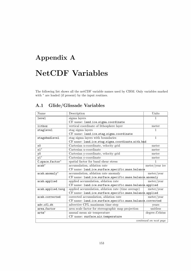
Appendix A
NetCDF Variables
The following list shows all the netCDF variable names used by CISM. Only variables markedwith ∗ are loaded (if present) by the input routines.
A.1 Glide/Glissade Variables
Name Description Units
level sigma layers 1CF name: land ice sigma coordinate
lithoz vertical coordinate of lithosphere layer meterstaglevel stag sigma layers 1
CF name: land ice stag sigma coordinate
stagwbndlevel stag sigma layers with boundaries 1CF name: land ice stag sigma coordinate with bnd
x0 Cartesian x-coordinate, velocity grid meterx1∗ Cartesian x-coordinate metery0 Cartesian y-coordinate, velocity grid metery1∗ Cartesian y-coordinate meterC space factor∗ spatial factor for basal shear stress 1acab∗ accumulation, ablation rate meter/year ice
CF name: land ice surface specific mass balance
acab anomaly∗ accumulation, ablation rate anomaly meter/yearCF name: land ice surface specific mass balance anomaly
acab applied applied accumulation, ablation rate meter/yearCF name: land ice surface specific mass balance applied
acab applied tavg applied accumulation, ablation rate (time average) meter/yearCF name: land ice surface specific mass balance applied
acab corrected corrected accumulation, ablation rate meter/yearCF name: land ice surface specific mass balance corrected
adv cfl dt advective CFL maximum time step yearsarea factor area scale factor for stereographic map projection unitlessartm∗ annual mean air temperature degree Celsius
CF name: surface air temperature
continued on next page
153
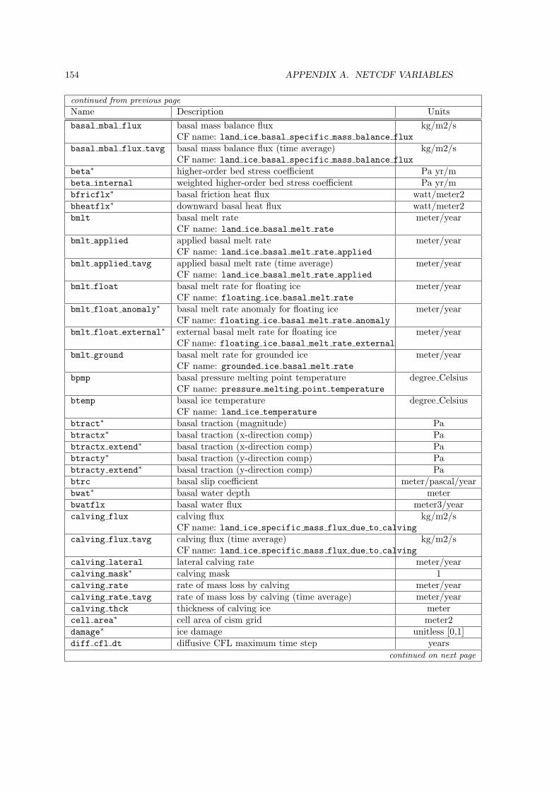
154 APPENDIX A. NETCDF VARIABLES
continued from previous page
Name Description Units
basal mbal flux basal mass balance flux kg/m2/sCF name: land ice basal specific mass balance flux
basal mbal flux tavg basal mass balance flux (time average) kg/m2/sCF name: land ice basal specific mass balance flux
beta∗ higher-order bed stress coefficient Pa yr/mbeta internal weighted higher-order bed stress coefficient Pa yr/mbfricflx∗ basal friction heat flux watt/meter2bheatflx∗ downward basal heat flux watt/meter2bmlt basal melt rate meter/year
CF name: land ice basal melt rate
bmlt applied applied basal melt rate meter/yearCF name: land ice basal melt rate applied
bmlt applied tavg applied basal melt rate (time average) meter/yearCF name: land ice basal melt rate applied
bmlt float basal melt rate for floating ice meter/yearCF name: floating ice basal melt rate
bmlt float anomaly∗ basal melt rate anomaly for floating ice meter/yearCF name: floating ice basal melt rate anomaly
bmlt float external∗ external basal melt rate for floating ice meter/yearCF name: floating ice basal melt rate external
bmlt ground basal melt rate for grounded ice meter/yearCF name: grounded ice basal melt rate
bpmp basal pressure melting point temperature degree CelsiusCF name: pressure melting point temperature
btemp basal ice temperature degree CelsiusCF name: land ice temperature
btract∗ basal traction (magnitude) Pabtractx∗ basal traction (x-direction comp) Pabtractx extend∗ basal traction (x-direction comp) Pabtracty∗ basal traction (y-direction comp) Pabtracty extend∗ basal traction (y-direction comp) Pabtrc basal slip coefficient meter/pascal/yearbwat∗ basal water depth meterbwatflx basal water flux meter3/yearcalving flux calving flux kg/m2/s
CF name: land ice specific mass flux due to calving
calving flux tavg calving flux (time average) kg/m2/sCF name: land ice specific mass flux due to calving
calving lateral lateral calving rate meter/yearcalving mask∗ calving mask 1calving rate rate of mass loss by calving meter/yearcalving rate tavg rate of mass loss by calving (time average) meter/yearcalving thck thickness of calving ice metercell area∗ cell area of cism grid meter2damage∗ ice damage unitless [0,1]diff cfl dt diffusive CFL maximum time step years
continued on next page
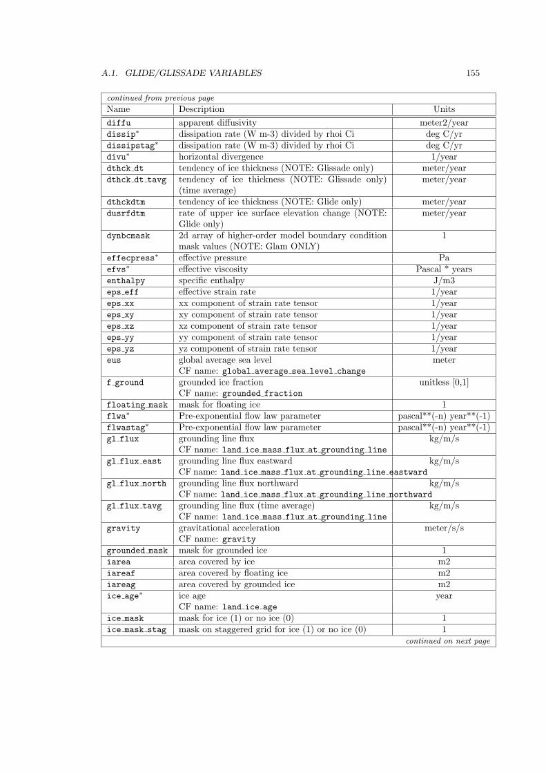
A.1. GLIDE/GLISSADE VARIABLES 155
continued from previous page
Name Description Units
diffu apparent diffusivity meter2/yeardissip∗ dissipation rate (W m-3) divided by rhoi Ci deg C/yrdissipstag∗ dissipation rate (W m-3) divided by rhoi Ci deg C/yrdivu∗ horizontal divergence 1/yeardthck dt tendency of ice thickness (NOTE: Glissade only) meter/yeardthck dt tavg tendency of ice thickness (NOTE: Glissade only)
(time average)meter/year
dthckdtm tendency of ice thickness (NOTE: Glide only) meter/yeardusrfdtm rate of upper ice surface elevation change (NOTE:
Glide only)meter/year
dynbcmask 2d array of higher-order model boundary conditionmask values (NOTE: Glam ONLY)
1
effecpress∗ effective pressure Paefvs∗ effective viscosity Pascal * yearsenthalpy specific enthalpy J/m3eps eff effective strain rate 1/yeareps xx xx component of strain rate tensor 1/yeareps xy xy component of strain rate tensor 1/yeareps xz xz component of strain rate tensor 1/yeareps yy yy component of strain rate tensor 1/yeareps yz yz component of strain rate tensor 1/yeareus global average sea level meter
CF name: global average sea level change
f ground grounded ice fraction unitless [0,1]CF name: grounded fraction
floating mask mask for floating ice 1flwa∗ Pre-exponential flow law parameter pascal**(-n) year**(-1)flwastag∗ Pre-exponential flow law parameter pascal**(-n) year**(-1)gl flux grounding line flux kg/m/s
CF name: land ice mass flux at grounding line
gl flux east grounding line flux eastward kg/m/sCF name: land ice mass flux at grounding line eastward
gl flux north grounding line flux northward kg/m/sCF name: land ice mass flux at grounding line northward
gl flux tavg grounding line flux (time average) kg/m/sCF name: land ice mass flux at grounding line
gravity gravitational acceleration meter/s/sCF name: gravity
grounded mask mask for grounded ice 1iarea area covered by ice m2iareaf area covered by floating ice m2iareag area covered by grounded ice m2ice age∗ ice age year
CF name: land ice age
ice mask mask for ice (1) or no ice (0) 1ice mask stag mask on staggered grid for ice (1) or no ice (0) 1
continued on next page
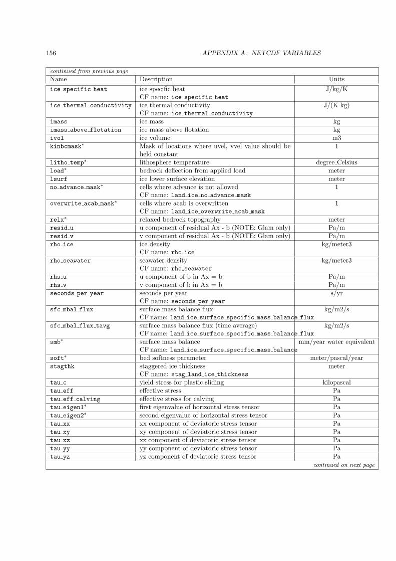
156 APPENDIX A. NETCDF VARIABLES
continued from previous page
Name Description Units
ice specific heat ice specific heat J/kg/KCF name: ice specific heat
ice thermal conductivity ice thermal conductivity J/(K kg)CF name: ice thermal conductivity
imass ice mass kgimass above flotation ice mass above flotation kgivol ice volume m3kinbcmask∗ Mask of locations where uvel, vvel value should be
held constant1
litho temp∗ lithosphere temperature degree Celsiusload∗ bedrock deflection from applied load meterlsurf ice lower surface elevation meterno advance mask∗ cells where advance is not allowed 1
CF name: land ice no advance mask
overwrite acab mask∗ cells where acab is overwritten 1CF name: land ice overwrite acab mask
relx∗ relaxed bedrock topography meterresid u u component of residual Ax - b (NOTE: Glam only) Pa/mresid v v component of residual Ax - b (NOTE: Glam only) Pa/mrho ice ice density kg/meter3
CF name: rho ice
rho seawater seawater density kg/meter3CF name: rho seawater
rhs u u component of b in Ax = b Pa/mrhs v v component of b in Ax = b Pa/mseconds per year seconds per year s/yr
CF name: seconds per year
sfc mbal flux surface mass balance flux kg/m2/sCF name: land ice surface specific mass balance flux
sfc mbal flux tavg surface mass balance flux (time average) kg/m2/sCF name: land ice surface specific mass balance flux
smb∗ surface mass balance mm/year water equivalentCF name: land ice surface specific mass balance
soft∗ bed softness parameter meter/pascal/yearstagthk staggered ice thickness meter
CF name: stag land ice thickness
tau c yield stress for plastic sliding kilopascaltau eff effective stress Patau eff calving effective stress for calving Patau eigen1∗ first eigenvalue of horizontal stress tensor Patau eigen2∗ second eigenvalue of horizontal stress tensor Patau xx xx component of deviatoric stress tensor Patau xy xy component of deviatoric stress tensor Patau xz xz component of deviatoric stress tensor Patau yy yy component of deviatoric stress tensor Patau yz yz component of deviatoric stress tensor Pa
continued on next page
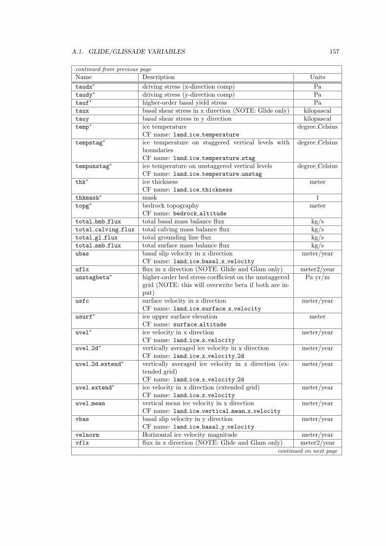
A.1. GLIDE/GLISSADE VARIABLES 157
continued from previous page
Name Description Units
taudx∗ driving stress (x-direction comp) Pataudy∗ driving stress (y-direction comp) Patauf∗ higher-order basal yield stress Pataux basal shear stress in x direction (NOTE: Glide only) kilopascaltauy basal shear stress in y direction kilopascaltemp∗ ice temperature degree Celsius
CF name: land ice temperature
tempstag∗ ice temperature on staggered vertical levels withboundaries
degree Celsius
CF name: land ice temperature stag
tempunstag∗ ice temperature on unstaggered vertical levels degree CelsiusCF name: land ice temperature unstag
thk∗ ice thickness meterCF name: land ice thickness
thkmask∗ mask 1topg∗ bedrock topography meter
CF name: bedrock altitude
total bmb flux total basal mass balance flux kg/stotal calving flux total calving mass balance flux kg/stotal gl flux total grounding line flux kg/stotal smb flux total surface mass balance flux kg/subas basal slip velocity in x direction meter/year
CF name: land ice basal x velocity
uflx flux in x direction (NOTE: Glide and Glam only) meter2/yearunstagbeta∗ higher-order bed stress coefficient on the unstaggered
grid (NOTE: this will overwrite beta if both are in-put)
Pa yr/m
usfc surface velocity in x direction meter/yearCF name: land ice surface x velocity
usurf∗ ice upper surface elevation meterCF name: surface altitude
uvel∗ ice velocity in x direction meter/yearCF name: land ice x velocity
uvel 2d∗ vertically averaged ice velocity in x direction meter/yearCF name: land ice x velocity 2d
uvel 2d extend∗ vertically averaged ice velocity in x direction (ex-tended grid)
meter/year
CF name: land ice x velocity 2d
uvel extend∗ ice velocity in x direction (extended grid) meter/yearCF name: land ice x velocity
uvel mean vertical mean ice velocity in x direction meter/yearCF name: land ice vertical mean x velocity
vbas basal slip velocity in y direction meter/yearCF name: land ice basal y velocity
velnorm Horizontal ice velocity magnitude meter/yearvflx flux in x direction (NOTE: Glide and Glam only) meter2/year
continued on next page
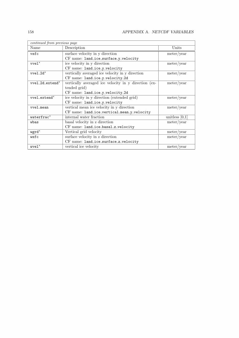
158 APPENDIX A. NETCDF VARIABLES
continued from previous page
Name Description Units
vsfc surface velocity in y direction meter/yearCF name: land ice surface y velocity
vvel∗ ice velocity in y direction meter/yearCF name: land ice y velocity
vvel 2d∗ vertically averaged ice velocity in y direction meter/yearCF name: land ice y velocity 2d
vvel 2d extend∗ vertically averaged ice velocity in y direction (ex-tended grid)
meter/year
CF name: land ice y velocity 2d
vvel extend∗ ice velocity in y direction (extended grid) meter/yearCF name: land ice y velocity
vvel mean vertical mean ice velocity in y direction meter/yearCF name: land ice vertical mean y velocity
waterfrac∗ internal water fraction unitless [0,1]wbas basal velocity in z direction meter/year
CF name: land ice basal z velocity
wgrd∗ Vertical grid velocity meter/yearwsfc surface velocity in z direction meter/year
CF name: land ice surface z velocity
wvel∗ vertical ice velocity meter/year
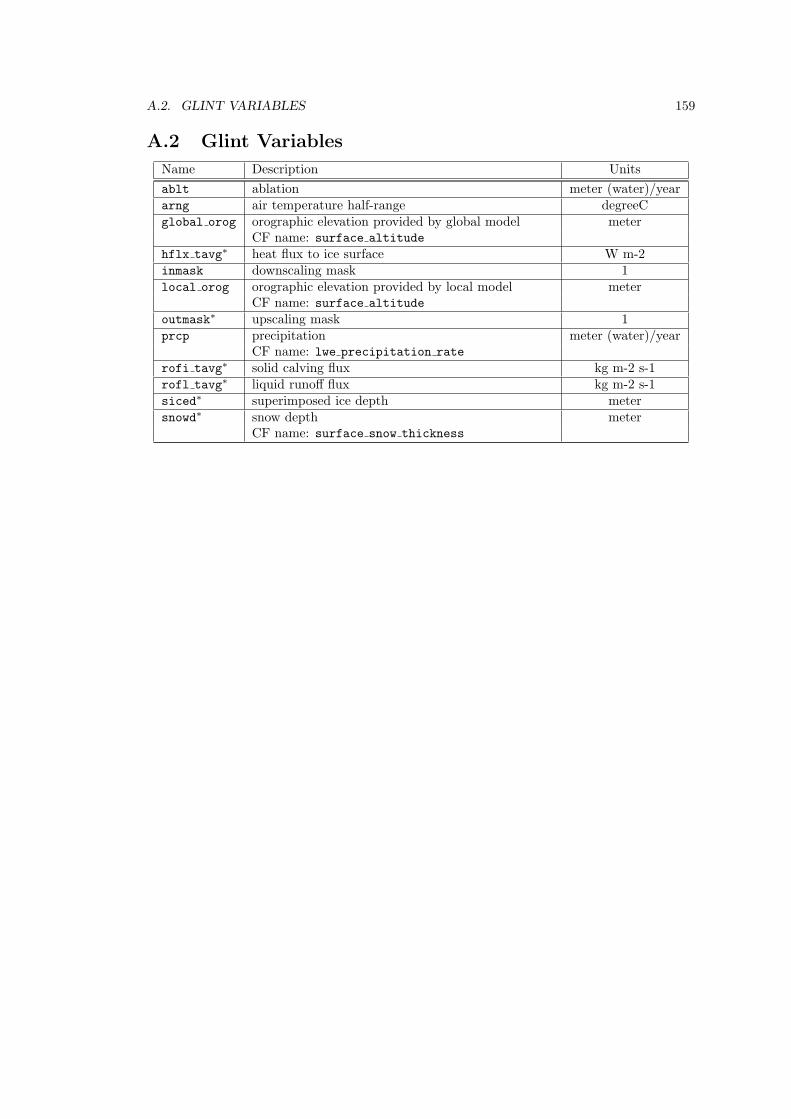
A.2. GLINT VARIABLES 159
A.2 Glint Variables
Name Description Units
ablt ablation meter (water)/yeararng air temperature half-range degreeCglobal orog orographic elevation provided by global model meter
CF name: surface altitude
hflx tavg∗ heat flux to ice surface W m-2inmask downscaling mask 1local orog orographic elevation provided by local model meter
CF name: surface altitude
outmask∗ upscaling mask 1prcp precipitation meter (water)/year
CF name: lwe precipitation rate
rofi tavg∗ solid calving flux kg m-2 s-1rofl tavg∗ liquid runoff flux kg m-2 s-1siced∗ superimposed ice depth metersnowd∗ snow depth meter
CF name: surface snow thickness

160 APPENDIX A. NETCDF VARIABLES
Appendix B
Input and Output (I/O)
B.1 NetCDF I/O
The netCDF1 library is used for platform-independent, binary file I/O. CISM uses the f90netCDF interface. Several source files are automatically generated from template files and avariable definition file using a python script. The netCDF files adhere to the CF convention2 fornaming climate variables. The netCDF files also store parameters used to define the geographicprojection.
B.1.1 Data structures
Information associated with each dataset is stored in the glimmer nc stat type. Variable anddimension IDs are retrived from the data set by using the relevant netCDF library calls. Meta-data (such as title, institution and comments) are stored in the derived type glimmer nc meta.
Input and output files are managed by two separate linked lists. Elements of the input filelist contain the number of available time slices and information describing which time slice(s)should be read. Output file elements describe how often data should be written and the currenttime.
B.1.2 Code generator
Much of the code needed to do netCDF I/O is repetitive and can therefore be automaticallygenerated. The code generator, generate ncvars.py, is written in python and produces sourcefiles from a template ncdf template.in and the variable definition file (Section B.1.3). Thetemplates are valid source files; the generator simply replaces special comments with the codegenerated from the variable file.
B.1.3 Variable definition file
All netCDF variables are defined in control files, MOD vars.def, where MOD is the name ofthe model subsystem. Variables can be modified/added by editing these files to provide I/Ofunctionality for additional variables beyond those listed in Appendix A. A common examplewould be to modify the file glide vars.def in ./libglide so that additional standard variablescan be treated as “loadable” on input, or so that other standard variables internal to the codecan be written to NetCDF output. Note that if MOD vars.def is modified, the CMake configurescript must be re-sourced before running “make” in order for those changes to be applied.
1http://www.unidata.ucar.edu/packages/netcdf/2http://cfconventions.org/
161
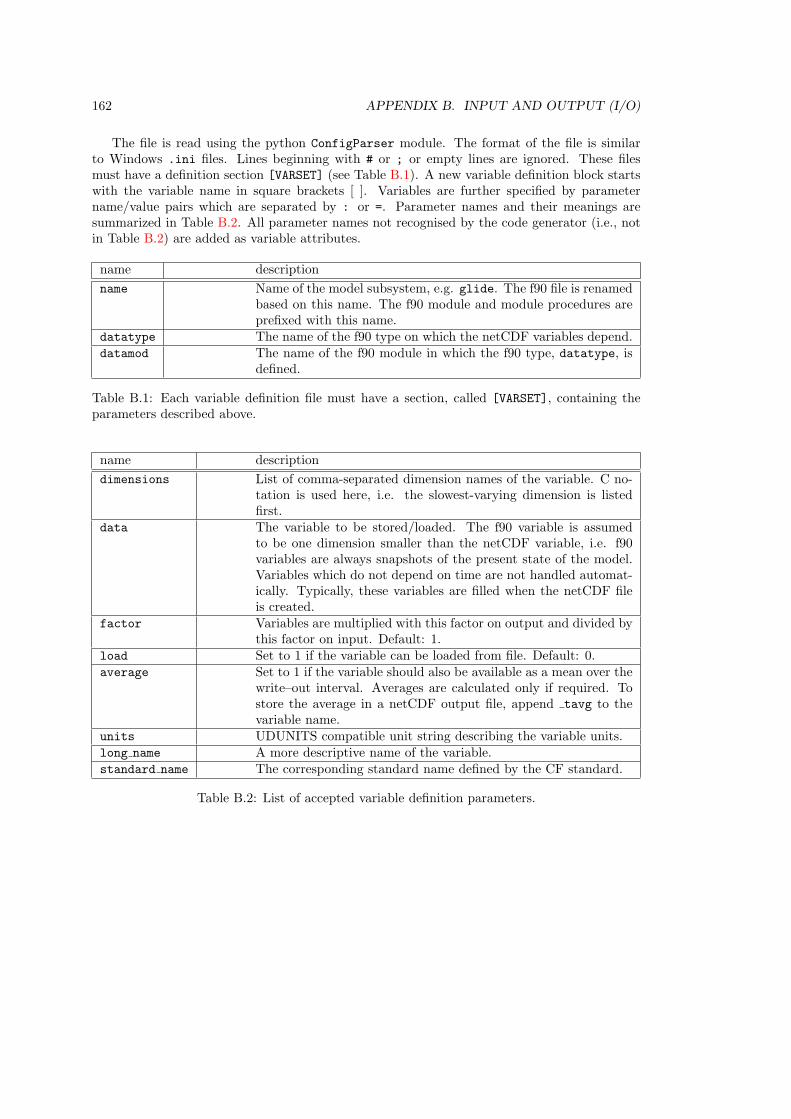
162 APPENDIX B. INPUT AND OUTPUT (I/O)
The file is read using the python ConfigParser module. The format of the file is similarto Windows .ini files. Lines beginning with # or ; or empty lines are ignored. These filesmust have a definition section [VARSET] (see Table B.1). A new variable definition block startswith the variable name in square brackets [ ]. Variables are further specified by parametername/value pairs which are separated by : or =. Parameter names and their meanings aresummarized in Table B.2. All parameter names not recognised by the code generator (i.e., notin Table B.2) are added as variable attributes.
name description
name Name of the model subsystem, e.g. glide. The f90 file is renamedbased on this name. The f90 module and module procedures areprefixed with this name.
datatype The name of the f90 type on which the netCDF variables depend.datamod The name of the f90 module in which the f90 type, datatype, is
defined.
Table B.1: Each variable definition file must have a section, called [VARSET], containing theparameters described above.
name description
dimensions List of comma-separated dimension names of the variable. C no-tation is used here, i.e. the slowest-varying dimension is listedfirst.
data The variable to be stored/loaded. The f90 variable is assumedto be one dimension smaller than the netCDF variable, i.e. f90variables are always snapshots of the present state of the model.Variables which do not depend on time are not handled automat-ically. Typically, these variables are filled when the netCDF fileis created.
factor Variables are multiplied with this factor on output and divided bythis factor on input. Default: 1.
load Set to 1 if the variable can be loaded from file. Default: 0.average Set to 1 if the variable should also be available as a mean over the
write–out interval. Averages are calculated only if required. Tostore the average in a netCDF output file, append tavg to thevariable name.
units UDUNITS compatible unit string describing the variable units.long name A more descriptive name of the variable.standard name The corresponding standard name defined by the CF standard.
Table B.2: List of accepted variable definition parameters.
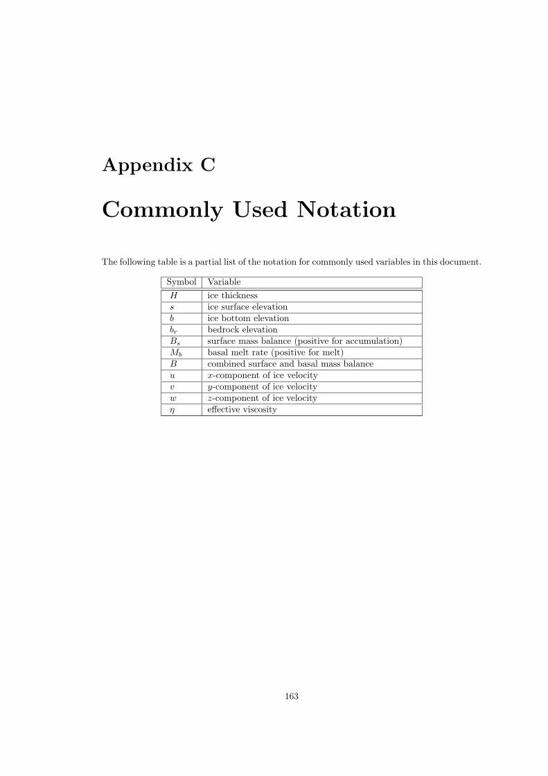
Appendix C
Commonly Used Notation
The following table is a partial list of the notation for commonly used variables in this document.
Symbol Variable
H ice thicknesss ice surface elevationb ice bottom elevationbr bedrock elevationBs surface mass balance (positive for accumulation)Mb basal melt rate (positive for melt)B combined surface and basal mass balanceu x-component of ice velocityv y-component of ice velocityw z-component of ice velocityη effective viscosity
163

164 APPENDIX C. COMMONLY USED NOTATION

Part III
Bibliography
165

Bibliography
T. Albrecht, M. Martin, M. Haseloff, R. Winkelmann, and A. Levermann. Parameterizationfor subgrid-scale motion of ice-shelf calving fronts. The Cryosphere, 5(1):35–44, 2011. doi:10.5194/tc-5-35-2011.
X. S. Asay-Davis, S. L. Cornford, G. Durand, B. K. Galton-Fenzi, R. M. Gladstone, G. H.Gudmundsson, T. Hattermann, D. M. Holland, D. Holland, P. R. Holland, D. F. Martin,P. Mathiot, F. Pattyn, and H. Seroussi. Experimental design for three interrelated marineice sheet and ocean model intercomparison projects: Mismip v. 3 (mismip+), isomip v. 2(isomip+) and misomip v. 1 (misomip1). Geosci. Model Dev., 9:2471–2497, 2016. doi: 10.5194/gmdd-9-2471-2016.
A. Aschwanden, G. Adalgeirsdottir, and C. Khroulev. Hindcasting to measure ice sheetmodel sensitivity to initial states. The Cryosphere, 7(4):1083–1093, 2013. doi: 10.5194/tc-7-1083-2013.
A. Aschwanden, M. A. Fahnestock, and M. Truffer. Complex greenland outlet glacier flowcaptured. Nat. Commun., 7, 2016. doi: 10.1038/ncomms10524.
R. Bindschadler. The importance of pressurized subglacial water in separation and sliding atthe glacier bed. J. Glaciol., 29:3–19, 1983.
H. Blatter. Velocity and stress fields in grounded glaciers - a simple algorithm for includingdeviatoric stress gradients. J. Glaciol., 41(138):333–344, 1995.
W.F. Budd, P.L. Keage, and N.A. Blundy. Empirical studies of ice sliding. J. Glaciol., 23(89):157–170, 1979.
Ed Bueler and Jed Brown. Shallow shelf approximation as a “sliding law” in a thermomechan-ically coupled ice sheet model. J. Geophys. Res., 114(F3):1–21, July 2009.
Ed Bueler, Craig S. Lingle, Jed A. Kallen-Brown, David N. Covey, and Latrice N. Bowman.Exact solutions and verification of numerical models for isothermal ice sheets. J. Glaciol., 51(173):291–306, 2005. doi: 10.3189/172756505781829449.
K. Cuffey and W. S. B. Paterson. The Physics of Glaciers. Butterworth-Heinneman, Amster-dam, 4th edition, 2010.
J. K. Dukowicz and J. R. Baumgardner. Incremental remapping as a transport/advectionalgorithm. J. Comput. Phys., 160:318–335, 2000.
J. K. Dukowicz, S. F. Price, and W. H. Lipscomb. Consistent approximations and boundaryconditions for ice-sheet dynamics from a principle of least action. J. Glaciol., 56(197):480–496,2010.
167
168 BIBLIOGRAPHY
O Gagliardini, T Zwinger, F Gillet-Chaulet, G Durand, L Favier, B De Fleurian, R Greve,M Malinen, C Martin, P Raback, J Ruokolainen, M Sacchettini, M Schafer, H Seddik, andJ Thies. Capabilities and performance of Elmer/Ice, a new-generation ice sheet model. Geosci.Model Dev., 6(4):1299–1318, 2013.
D. N. Goldberg. A variationally derived, depth-integrated approximation to a higher-order glaciological flow model. J. Glaciol., 57(201):157–170, 2011. doi: 10.3189/002214311795306763.
M. K. M. Hagdorn. Reconstruction of the Past and Forecast of the Future European and BritishIce Sheets and Associated Sea Level Change. PhD thesis, University of Edinburgh, 2003.
P Halfar. On the dynamics of the ice sheets 2. J. Geophys. Res., 88(C10):6043–6051, 1983.
R.C.A. Hindmarsh. A numerical comparison of approximations to the stokes equations used inice sheet and glacier modeling. J. Geophys. Res., 109, 2004. doi: 10.1029/2003JF000065.
J. R. Holton. An Introduction to Dynamic Meteorology, volume 48 of International GeophysicsSeries. Academic Press, New York, 3rd edition, 1992.
K. H. Huebner, D. L. Dewhirst, D. E. Smith, and T. G. Byrom. The Finite Element Methodfor Engineers. Wiley, New York, 4th edition, 2001.
T.J.R. Hughes. The Finite Element Method: Linear Static and Dynamic Finite Element Anal-ysis. Dover Civil and Mechanical Engineering. Dover, Mineola, New York, 1st edition, 2000.
K. Hutter. Theoretical Glaciology. Mathematical Approaches to Geophysics. D. Reidel Publish-ing Company, Dordrecht, Boston, Lancaster, 1983.
P. Huybrechts. A three–dimensional time–dependent numerical model for polar ice sheets; somebasic testing with a stable and efficient finite difference scheme. Technical report, GeografischInstituut, Vrije Universiteit Brussel, Belgium, 1986.
Philippe Huybrechts, Tony Payne, and The EISMINT Intercomparison Group. The EISMINTbenchmarks for testing ice–sheet models. Ann. Glaciol., 23:1–12, 1996.
I Joughin, B Smith, IM Howat, T Scambos, and T Moon. Measures greenland ice sheet velocitymap from insar data. National Snow and Ice Data Center., Boulder, Colorado USA. doi:nsidc-0478.001, 2010.
Nina Kirchner, Kolumban Hutter, Martin Jakobsson, and Richard Gyllencreutz. Capabili-ties and limitations of numerical ice sheet models: a discussion for Earth-scientists andmodelers. Quat. Sci. Rev., 30(25-26):3691–3704, December 2011. ISSN 02773791. doi:10.1016/j.quascirev.2011.09.012.
K. Lambeck and S. M. Nakiboglu. Seamount loading and stress in the ocean lithosphere. J.Geophys. Res., 85:6403–6418, 1980.
G. R. Leguy, X. S. Asay-Davis, and W. H. Lipscomb. Parameterization of basal friction neargrounding lines in a one-dimensional ice sheet model. The Cryosphere, 8(4):1239–1259, July2014. ISSN 1994-0424. doi: 10.5194/tc-8-1239-2014.
Wei Leng, Lili Ju, Max Gunzburger, Stephen Price, and Todd Ringler. A parallel high-orderaccurate finite element nonlinear Stokes ice sheet model and benchmark experiments. J.Geophys. Res., 117(F1), 2012.
W. H. Lipscomb and E. C. Hunke. Modeling sea ice transport using incremental remapping.Mon. Wea. Rev., 132:1341–1354, 2004.
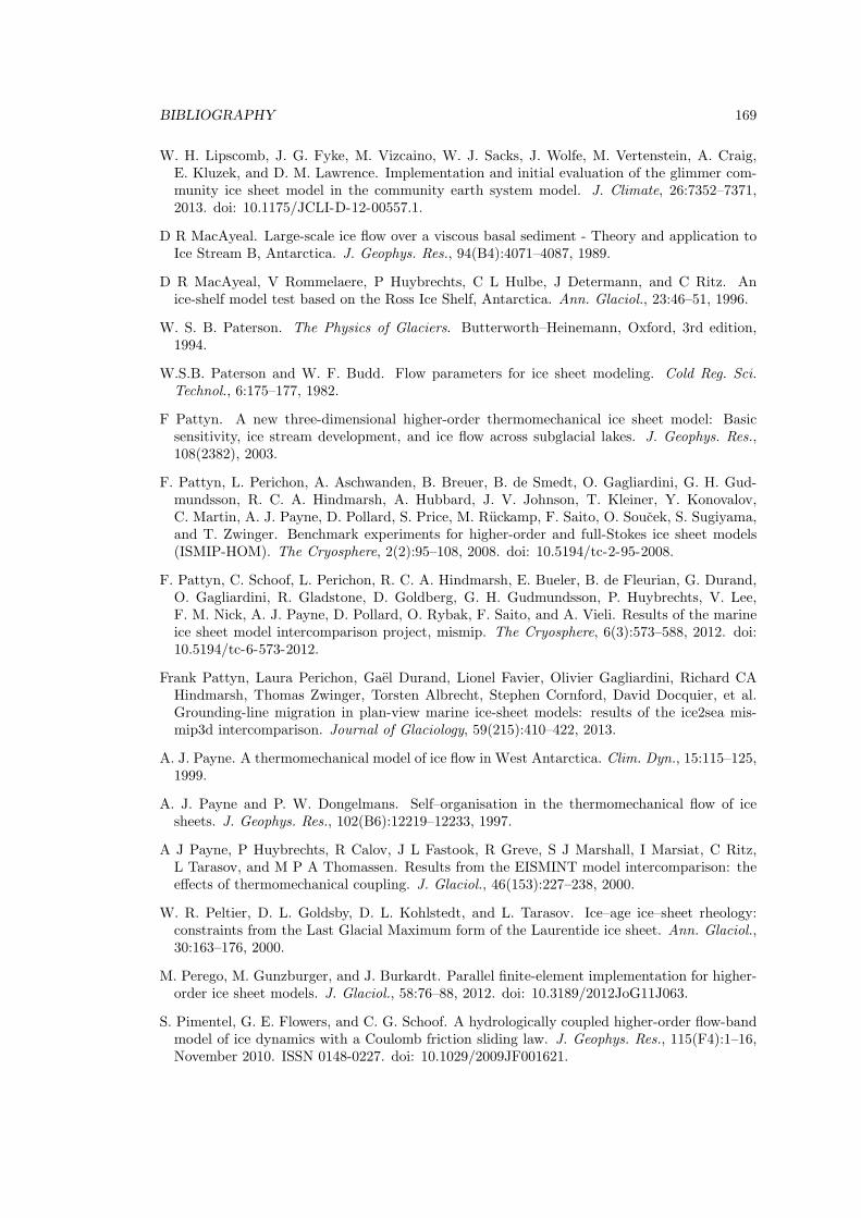
BIBLIOGRAPHY 169
W. H. Lipscomb, J. G. Fyke, M. Vizcaino, W. J. Sacks, J. Wolfe, M. Vertenstein, A. Craig,E. Kluzek, and D. M. Lawrence. Implementation and initial evaluation of the glimmer com-munity ice sheet model in the community earth system model. J. Climate, 26:7352–7371,2013. doi: 10.1175/JCLI-D-12-00557.1.
D R MacAyeal. Large-scale ice flow over a viscous basal sediment - Theory and application toIce Stream B, Antarctica. J. Geophys. Res., 94(B4):4071–4087, 1989.
D R MacAyeal, V Rommelaere, P Huybrechts, C L Hulbe, J Determann, and C Ritz. Anice-shelf model test based on the Ross Ice Shelf, Antarctica. Ann. Glaciol., 23:46–51, 1996.
W. S. B. Paterson. The Physics of Glaciers. Butterworth–Heinemann, Oxford, 3rd edition,1994.
W.S.B. Paterson and W. F. Budd. Flow parameters for ice sheet modeling. Cold Reg. Sci.Technol., 6:175–177, 1982.
F Pattyn. A new three-dimensional higher-order thermomechanical ice sheet model: Basicsensitivity, ice stream development, and ice flow across subglacial lakes. J. Geophys. Res.,108(2382), 2003.
F. Pattyn, L. Perichon, A. Aschwanden, B. Breuer, B. de Smedt, O. Gagliardini, G. H. Gud-mundsson, R. C. A. Hindmarsh, A. Hubbard, J. V. Johnson, T. Kleiner, Y. Konovalov,C. Martin, A. J. Payne, D. Pollard, S. Price, M. Ruckamp, F. Saito, O. Soucek, S. Sugiyama,and T. Zwinger. Benchmark experiments for higher-order and full-Stokes ice sheet models(ISMIP-HOM). The Cryosphere, 2(2):95–108, 2008. doi: 10.5194/tc-2-95-2008.
F. Pattyn, C. Schoof, L. Perichon, R. C. A. Hindmarsh, E. Bueler, B. de Fleurian, G. Durand,O. Gagliardini, R. Gladstone, D. Goldberg, G. H. Gudmundsson, P. Huybrechts, V. Lee,F. M. Nick, A. J. Payne, D. Pollard, O. Rybak, F. Saito, and A. Vieli. Results of the marineice sheet model intercomparison project, mismip. The Cryosphere, 6(3):573–588, 2012. doi:10.5194/tc-6-573-2012.
Frank Pattyn, Laura Perichon, Gael Durand, Lionel Favier, Olivier Gagliardini, Richard CAHindmarsh, Thomas Zwinger, Torsten Albrecht, Stephen Cornford, David Docquier, et al.Grounding-line migration in plan-view marine ice-sheet models: results of the ice2sea mis-mip3d intercomparison. Journal of Glaciology, 59(215):410–422, 2013.
A. J. Payne. A thermomechanical model of ice flow in West Antarctica. Clim. Dyn., 15:115–125,1999.
A. J. Payne and P. W. Dongelmans. Self–organisation in the thermomechanical flow of icesheets. J. Geophys. Res., 102(B6):12219–12233, 1997.
A J Payne, P Huybrechts, R Calov, J L Fastook, R Greve, S J Marshall, I Marsiat, C Ritz,L Tarasov, and M P A Thomassen. Results from the EISMINT model intercomparison: theeffects of thermomechanical coupling. J. Glaciol., 46(153):227–238, 2000.
W. R. Peltier, D. L. Goldsby, D. L. Kohlstedt, and L. Tarasov. Ice–age ice–sheet rheology:constraints from the Last Glacial Maximum form of the Laurentide ice sheet. Ann. Glaciol.,30:163–176, 2000.
M. Perego, M. Gunzburger, and J. Burkardt. Parallel finite-element implementation for higher-order ice sheet models. J. Glaciol., 58:76–88, 2012. doi: 10.3189/2012JoG11J063.
S. Pimentel, G. E. Flowers, and C. G. Schoof. A hydrologically coupled higher-order flow-bandmodel of ice dynamics with a Coulomb friction sliding law. J. Geophys. Res., 115(F4):1–16,November 2010. ISSN 0148-0227. doi: 10.1029/2009JF001621.
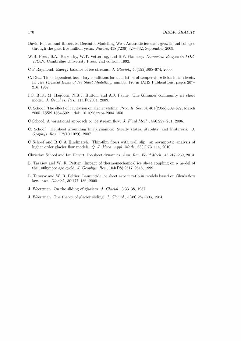
170 BIBLIOGRAPHY
David Pollard and Robert M Deconto. Modelling West Antarctic ice sheet growth and collapsethrough the past five million years. Nature, 458(7236):329–332, September 2009.
W.H. Press, S.A. Teukolsky, W.T. Vetterling, and B.P. Flannery. Numerical Recipes in FOR-TRAN. Cambridge University Press, 2nd edition, 1992.
C F Raymond. Energy balance of ice streams. J. Glaciol., 46(155):665–674, 2000.
C. Ritz. Time dependent boundary conditions for calculation of temperature fields in ice sheets.In The Physical Basis of Ice Sheet Modelling, number 170 in IAHS Publications, pages 207–216, 1987.
I.C. Rutt, M. Hagdorn, N.R.J. Hulton, and A.J. Payne. The Glimmer community ice sheetmodel. J. Geophys. Res., 114:F02004, 2009.
C. Schoof. The effect of cavitation on glacier sliding. Proc. R. Soc. A, 461(2055):609–627, March2005. ISSN 1364-5021. doi: 10.1098/rspa.2004.1350.
C Schoof. A variational approach to ice stream flow. J. Fluid Mech., 556:227–251, 2006.
C. Schoof. Ice sheet grounding line dynamics: Steady states, stability, and hysteresis. J.Geophys. Res, 112(10.1029), 2007.
C Schoof and R C A Hindmarsh. Thin-film flows with wall slip: an asymptotic analysis ofhigher order glacier flow models. Q. J. Mech. Appl. Math., 63(1):73–114, 2010.
Christian Schoof and Ian Hewitt. Ice-sheet dynamics. Ann. Rev. Fluid Mech., 45:217–239, 2013.
L. Tarasov and W. R. Peltier. Impact of thermomechanical ice sheet coupling on a model ofthe 100kyr ice age cycle. J. Geophys. Res., 104(D8):9517–9545, 1999.
L. Tarasov and W. R. Peltier. Laurentide ice sheet aspect ratio in models based on Glen’s flowlaw. Ann. Glaciol., 30:177–186, 2000.
J. Weertman. On the sliding of glaciers. J. Glaciol., 3:33–38, 1957.
J. Weertman. The theory of glacier sliding. J. Glaciol., 5(39):287–303, 1964.