City, Culture and Society 3 (2012) 189–200

Contents lists available at SciVerse ScienceDirect

City, Culture and Society

journal homepage: www.elsevier .com/locate /ccs

The impact of professional sports facilities on housing values: Evidencefrom census block group data

Xia Feng a, Brad R. Humphreys b,⇑a College of William and Mary, Virginia, United Statesb University of Alberta, Cananda

a r t i c l e i n f o a b s t r a c t

Article history:Received 5 February 2012Received in revised form date 23 June 2012Accepted 25 June 2012Available online 31 July 2012

Keywords:Spatial dependenceSports facilityResidential property value

1877-9166/$ - see front matter � 2012 Elsevier Ltd. Ahttp://dx.doi.org/10.1016/j.ccs.2012.06.017

⇑ Corresponding author. Address: Department of Ecton, AB, Canada T6G 2H4. Tel.: +1 780 492 5143; fax:

E-mail address: brad.humphreys@ualberta.ca (B.R.1 Alternatively, public subsidies may continue to be

sports leagues have significantly more bargaining pexercise monopoly power by keeping viable markets bowners can exploit this to extract subsidies from cities

We estimate the effect of proximity on residential property values in US cities using a hedonic housingprice model with spatial autocorrelation. Estimates based on all 1990 and 2000 Census block groupswithin five miles of every NFL, NBA, MLB, and NHL facility in the US suggest that the median house valuein block groups is higher in block groups closer to facilities, suggesting that positive externalities fromprofessional sports facilities may be capitalized into residential real estate prices. The existence of exter-nal benefits may justify some of the large public subsidies for construction and operation of professionalsports facilities.

� 2012 Elsevier Ltd. All rights reserved.

Introduction

Despite a lack of evidence that sports facilities generatetangible positive economic benefits, cities continue to sub-sidize the construction of new sports facilities in order toattract new teams or keep existing ones. The persistentsubsidies indicate that professional sports facilities maygenerate some benefits and suggest looking beyond directeconomic impact, in terms of income, jobs, and taxes, forevidence.1 One place to look for evidence of intangible ben-efits is in the value of fixed assets like real estate. The valueof some non-market public goods like open space, good airquality, high quality schools, etc., appears to be capitalizedinto housing values and reflected in wages in the form ofcompensating differentials, based on empirical estimatesfrom standard hedonic models. If air quality and green spaceaffect wages and housing values, then non-economic bene-fits generated by sports facilities and teams might also becapitalized into these prices.

The literature examining the economic impact of sportscontains relatively few studies that examine the effect of

ll rights reserved.

onomics, 8-14 Tory, Edmon-+1 780 492 3300.Humphreys).provided because monopoly

ower than cities. If leaguesereft of teams, existing teamby threatening to move.

sports facilities on housing values, even though intangiblebenefits are frequently mentioned as potentially importantbenefits generated by sports facilities. Only a handful of pa-pers investigate the effects of sports facilities on housingvalues or rents: Ahlfeldt and Kavetsos (2011), Ahlfeld andMaennig (2010), Carlino and Coulson (2004), Dehring, Dep-ken, and Ward (2007), Kiel, Matheson, and Sullivan (2010)and Tu (2005). We examine the effects of spatial proximityto a sports facility on housing values using cross-sectionaldata from the 1990 and 2000 United States Censuses. Thisresearch differs from existing studies in several ways. First,it uses data from a relatively small geographic scope- cen-sus block group level data. This has several advantages overmore aggregated data in that it allows us to control for spa-tial heterogeneity across cities. The effect of spatial proxim-ity to a sports facility on housing values can also beexamined more precisely in block group level data becausea variable reflecting the distance from a facility to eachblock group can be incorporated in the empirical model.Second, the sample contains data from all MetropolitanStatistical Areas (MSAs) with a franchise in any of the fourmajor professional sports leagues, the National FootballLeague (NFL), the National Basketball Association (NBA),the National Hockey League (NHL) and Major League Base-ball (MLB). The effect of different types of sports facilitieson housing values may vary because of different eventscheduling patterns for the facilities. For example, amongthe four professional sports facilities, NBA and/or HNL

190 X. Feng, B.R. Humphreys / City, Culture and Society 3 (2012) 189–200

arenas and MLB stadiums are used more frequently thanNFL stadiums because there are at least 41 NBA and NHLregular season home games a year and 81 MLB regular sea-son home games a year but only 8 NFL regular season homegames. Most facilities also hose some pre-season games ona regular basis. Moreover, arenas host many other activitieslike concerts and trade shows, and some arenas are hometo both NBA and NHL teams, which may enhance theirdesirability. Finally, our empirical methodology explicitlycontrols for spatial dependence in the data by accountingfor spatial autocorrelation. This important element hasbeen ignored in most of the existing literature on the spa-tial economic impact of professional sports facilities. Wefind evidence that the median residential house value in acensus block group decreases as the block group gets far-ther from a sports facility, even after controlling for blockgroup characteristics and spatial dependence in the data.This suggests that professional sports facilities may gener-ate intangible benefits that are capitalized in housingvalues.

Related literature

A few papers have examined the effect of sports facilitieson rents and property values. Carlino and Coulson (2004)found evidence that NFL teams and facilities generatenon-economic benefits in central cities and their associatedMSAs. Given that professional sports are, at some level, anon-excludable public good, Carlino and Coulson (2004)posited that the intangible benefits from the NFL manifestthemselves as compensating differentials the same wayas other contributors to the quality of life in a community,such as clean air, low crime, and pleasant weather. Citiesthat gain an NFL team will have higher quality of life thancities that do not, producing higher rents or lower wages.Carlino and Coulson (2004) estimated two hedonic pricemodels, one for housing rents and the other for wages,using data from 53 of the 60 largest MSAs in 1993 and1999, at three different levels of geographic aggregation:central city level, MSA level, and Consolidated MetropolitanStatistical Area (CMSA) level. Their results indicated thatthe presence of an NFL franchise raised rent by approxi-mately 8% in central cities. Unlike other studies using hedo-nic models to measure the effects of attributes on housingprices in a specific location with individual housing data,this study was the first to employ cross-sectional dataacross major central cities and their associated MSAs usingdata from the American Housing Survey.

Carlino and Coulson (2004) did not address any potentialnegative effects generated by an NFL franchise on rent. Pro-fessional sports facilities may generate negative externali-ties because they also produce disamenities, such astraffic jams, noise, and trash. The net effect of sports facili-ties on housing values depends on the relative size of thepositive and negative effects. If the positive effect domi-nates negative effect, then the net effect will be positive.In other words, the sign of the net effect cannot be deter-mined a priori.

Carlino and Coulson’s (2004) estimates are not robust tochanges in the geographic scope of the sample, suggestingthat intangible benefits may exhibit spatial heterogeneity.The effect of sports facilities located in the urban core of

cities may not spillover substantially to suburban areas.While suburban residents might derive benefits from livingin a MSA that is home to a team, these benefits may dimin-ish as the distance from the facility increases. So expandingthe geographic scope from central cities to MSA, or evenbigger CMSA, without controlling for spatial heterogeneitymay not identify the effects of the presence of an NFL teamon property values.

Spatial heterogeneity has been shown to be an impor-tant element of urban housing markets. Spatial heterogene-ity exists in cities because housing values depend onsurrounding amenities like good school quality and lowcrime rates. Variation in these amenities across spacemay affect housing values. So distance from a sports facilitycan be expected to affect housing values. We hypothesizethat the economic impacts on housing values would behigher near a sports facility than far from the facility, anddecline as the distance from the facility increases, givenother things equal.

Kiel et al. (2010) performed a study similar to Carlinoand Coulson (2004), but examined housing prices, not rent.This study also used data from the American Housing Sur-vey in 1993 and 1999. Like Carlino and Coulson (2004), Kielet al. (2010) estimated a hedonic model where the log ofthe owner-reported housing value was the dependent var-iable. They did not account for spatial dependence in thedata. Kiel et al. (2010) found no relationship between resi-dential housing values and proximity to NFL stadiums, aftercontrolling for other factors affecting housing values.

Four similar case studies on the spatial economic impactof sports facilities have recently been published: Ahlfeldtand Kavetsos (2011), Ahlfeldt and Maennig (2010), Dehringet al. (2007), and Tu (2005). The first two examined the ef-fects of an NFL stadium on property values while the thirdand fourth examined the effect of sports stadiums on prop-erty values in Europe. Tu (2005) analyzed the impact of Fe-dEx Field, home of NFL’s Washington Redskins, on housingvalues in Price George’s County, Maryland. Dehring et al.(2007) analyzed the impacts of announcements about a po-tential football stadium for the Dallas Cowboys in Arling-ton, Texas on housing values. Ahlfeld and Maennig (2010)analyzed the effect of three stadiums on assessed land va-lue in Berlin. Ahlfeldt and Kavetsos (2011) analyzed the ef-fect of the new Wembley stadium and Emirates stadium,on property values in London. These four papers reacheddifferent conclusions. Tu (2005) found a positive effect ofFedEx Field on housing values within three miles of the sta-dium; Ahlfeld and Maennig (2007) found both positive andnegative effects of stadiums on housing values in Berlin;Dehring et al. (2007) found a negative aggregate impactof the three announcements on property values. Ahlfeldtand Kavetsos (2011) found a positive effect of new stadiumannouncements on property values.

Tu (2005) did not account for spatial dependence, whichexists in spatial cross-sectional data, but instead modeledspatial proximity to FedEx Field by including a distancevariable and three distance dummy variables indicating ifthe property is located in ‘‘impact areas” with three differ-ent radii: one-mile, two-miles, and three-miles..

Tu (2005) estimated a series of standard hedonic modelsto measure the price differentials between houses locatedin close proximity to FedEx Field and those with similar

X. Feng, B.R. Humphreys / City, Culture and Society 3 (2012) 189–200 191

attributes but located at a distance from the stadium, andfound that houses within a one-mile radius from the sta-dium are priced lower than comparable units outside thethree-mile impact area. Tu (2005) also used a difference-in-difference approach to examine changes in the impactof FedEx Field on property values over three time periods:pre-development, development, and post-development.

Dehring et al. (2007) investigated two sets of stadiumannouncements concerning a new stadium for the NFL’sDallas Cowboys: a proposal to build a new stadium in Dal-las Fair Park which was ultimately abandoned; and a pro-posal to build a stadium in Arlington that wasundertaken. Dehring et al. (2007) employed a standard he-donic housing price model and a difference-in-differenceapproach to estimate the effects of these announcementson nearby residential property values. For the Dallas FairPark case, they found that property values increased nearDallas Fair Park after the announcement of the new sta-dium proposal. However, in Dallas County, which wouldhave paid for the stadium with increased sales taxes, resi-dential property values decreased after the announcement.These patterns reversed when the proposal was aban-doned. Three additional announcements concerning theproposed stadium in Arlington all had a negative impacton property values, but each was individually insignificant.The aggregate impact of the three announcements wasnegative and statistically significant. The accumulated netimpact corresponded to an approximate 1.5% decline inproperty values in Arlington, which was almost equal tothe anticipated household sales tax burden.

Again, both models in these two papers may be misspec-ified due to their failure to correct for spatial autocorrela-tion, leading to biased estimates. By explicitly accountingfor spatial autocorrelation, this study should produce unbi-ased and consistent estimates of the effect of sports facili-ties on housing values.

Alhfeldt and Maennig (2010) examined the effect ofthree multipurpose sports facilities on property values inBerlin. This case study is of considerable interest, as thesefacilities were built as urban redevelopment anchors inblighted neighborhoods. This study controlled for spatialdependence in the data. Alhfeldt and Maennig (2007) pres-ent evidence that sports facilities raise the assessed value ofsome properties within 3000 m of sports facilities, althoughthe impact declines with distance and the data also containsome evidence of a negative impact.

Some recent empirical evidence suggests that the non-pecuniary impacts of professional sports teams and facili-ties may vary across space (Coates & Humphreys, 2005).By analyzing voting on subsidies for professional sportsfacilities in two cities, Houston, Texas and Green Bay,Wisconsin, Coates and Humphreys (2005) found that votersliving in close proximity to facilities tend to favor subsidiesmore than voters living farther from the facilities. Also theyshowed precincts with more renters in Green Bay cast alarge share of ‘‘yes” votes for a subsidy for Lambeau Fieldwhile precincts with more renters in Houston cast a smallershare of ‘‘yes” votes for subsidies for a new basketballarena, which is consistent with Carlino and Coulson(2004) result in that it suggests a relationship betweenrenters and benefits from sports. This evidence indicatesthat the benefits generated by professional sports are

distributed unevenly not only across space within one citybut also across cities and implies the existence of spatialheterogeneity both within a city and across cities.

In summary, the existing literature contains some evi-dence that professional sports facilities generate externali-ties. The net effect of these externalities can be eitherpositive or negative. The existing evidence is based on de-tailed case studies of specific cities and facilities, and mostdoes not account for spatial dependence in the data. We ex-tend this literature by developing a comprehensive data setcontaining observations from many cities containing awide variety of sports facilities. We also extend the com-monly used hedonic housing price model to include spatialautocorrelation, a common feature in these data.

Empirical model

The standard hedonic housing price model relates themarket value of a residential property, usually measuredby sales price, to measures of housing unit attributes andneighborhood characteristics that determine the propertyvalues. When estimating a hedonic housing price model,an empirical researcher faces a choice among a number ofpossible functional forms for the empirical model. Theexisting literature uses linear functional forms (Palmquist,1984), semi-log functional forms (Carlino & Coulson,2004; Kiel et al., 2010), and log–log functional forms (Basu& Thibodeau, 1998). Each has advantages and disadvan-tages. For example, from an economic perspective, boththe log-linear and log–log forms permit the marginal impli-cit price of a particular attribute to vary across the observa-tions while the linear form forces a constant effect. Theadvantage of the linear form is that it is intuitive and pro-vides a direct estimate of the marginal implicit price of anattribute- the coefficient estimate on the attribute variablein the equation. The empirical hedonic model specificationused here is

Y ¼ aþ Xbþ e ð1Þ

where Y denotes an nx1 vector of housing values or log ofthe housing values, X is an nxk matrix of explanatory vari-ables representing housing structure attributes, individualsports facility characteristics, and locational attributes.Some variables in X are expressed in log forms. X is assumedto be uncorrelated with the error term e. a and b are vectorsof unknown parameters to be estimated. e is the standardrandom error term, which is uncorrelated with the explan-atory variables, with mean zero and variance constant.

Spatial autocorrelation

Spatial autocorrelation can be loosely defined as thecoincidence of value similarity and locational similarity(Anselin & Bera, 1998). Formally, spatial autocorrelationcan be expressed by the moment condition

Covðyi; yjÞ ¼ EðyiyjÞ � EðyiÞ � EðyjÞ–0 for i–j ð2Þ

where i and j refer to individual locations, yi and yj refer tothe values of a random variable at that location. Spatialautocorrelation can be positive where similar values (highor low) for a random variable tend to cluster in space or neg-ative where locations tend to be surrounded by neighbors

192 X. Feng, B.R. Humphreys / City, Culture and Society 3 (2012) 189–200

with very dissimilar values. Of the two types, positivespatial autocorrelation is more intuitive and is observedmuch more in reality than negative spatial autocorrelation.Spatial autocorrelation exists in cross-sectional data be-cause the variables examined share locational characteris-tics. Housing prices are spatially autocorrelated for thesame reason. Economists have long called attention to spa-tial autocorrelation when evaluating housing prices (Basu &Thibodeau, 1998; Can, 1992; Dubin, 1992; Kim, Phipps, andAnselin, 2003). Despite the recent advances in spatial dataanalysis and spatial econometrics (Anselin, 1988, 2003a;Anselin, Florax, and Rey, 2004), spatial autocorrelation hasnot been considered in existing hedonic housing studies ofthe impacts of spatial facilities. The existence of spatialautocorrelation in the data set implies a loss of information.By including a spatial lagged dependent variable or errorterm into the model, the loss of information can be explic-itly addressed (Anselin & Bera, 1998).

A crucial issue in modeling spatial autocorrelation is todefine the locations for which the values of the equation er-ror term are correlated, i.e., neighbors. Neighbors can bedefined by both geographical features, e.g., distance, conti-guity, and demographic or economic characteristics, e.g.,population density, trade flow. However, house prices areassumed to capitalize the locational amenities which maybe spatially autocorrelated. Therefore, the identification ofneighbors for observations on housing prices should bebased on geographic features.

Spatial lags

In general, spatial lag models are analogous to autore-gressive model used in time-series analysis. But there isan important distinction between these two models. Inspatial data, the autoregressive term induces simultaneitydue to the two-way interaction among neighbors, i.e., thespatial shift operator or spatial lag operator takes formsof both yi�1 and yi+1 , while there is no counterpart to timeseries data.

Following Anselin (1988), the formal spatial lag hedonicmodel, or spatial autoregressive (SAR) lag model can berepresented as follows (Anselin, 1988):

y ¼ qWyþ Xbþ e ð3Þwhere q is the spatial autoregressive parameter with |q| < 1,W is an n � n row-standardized spatial weights matrix thatrepresents the neighbor structure with spatial lag Wy as aweighted average of neighboring values, and the other vari-ables are as in Eq. (1). After some manipulation, the reducedform of the spatial lag model can be expressed

y ¼ ðI � qWÞ�1Xbþ ðI � qWÞ�1e ð4Þwhere the ‘‘Leontief Inverse” ðI � qWÞ�1 links the depen-dent variable y to all the xi in the system through a spatialmultiplier. Note that expanding the ‘‘Leontief Inverse” ma-trix leads to an expanded form given that |q| < 1 and wij,the element of W, is less than 1 for row-standardized spatialweights:

ðI � qWÞ�1 ¼ I þ qW þ q2W2 þ ::: ð5Þwhere each observation of dependent variable is linked toall observations of the explanatory variables through this

spatial multiplier. In addition, Eqs. (4) and (5) show howthe dependent variable y at location i is related to the errorterms at all locations in the system through the same spatialmultiplier in the SAR process. So this SAR process generatesa global range of spillovers, which is referred as a type ofglobal autocorrelation since it relates all the locations inthe system to each other (Anselin, 2003b). This SAR processwell captures the features of housing market in that thereare neighboring spillover effects on houses each other dueto shared neighborhood amenities. So each house price af-fects all the other houses in the neighborhood, but with dis-tance decay. This simultaneity due to the two-way spatialinteraction makes the spatial lag term Wy correlated withthe equation error term, which makes the OLS estimatorsbiased and inconsistent. Anselin (1988) develops maximumlikelihood and instrumental variables estimators to correctfor this problem. The following section discusses theseestimators.

Spatial errors

There are two different specifications for the errorterms: spatial autoregressive errors and spatial movingaverage errors. Accordingly, two types of spatial error mod-els can be specified. The spatial autoregressive (SAR) errormodel is similar to Eq. (3) but with a spatial lag in the errorterm (Anselin, 1988):

e ¼ kWeþ u ð6Þwhere k is the spatial autoregressive parameter with |k| < 1,W is the weights matrix, and u is a vector of i.i.d. errors. Likethe spatial lag model solved for y, the above error term canbe expressed:

e ¼ ½I � kW��1u ð7Þwhere similarly, for |k| < 1 and wij < 1, the expansion of the‘‘Leontief Inverse” matrix is:

ðI � kWÞ�1 ¼ I þ kW þ k2W2 þ ::: ð8ÞThe variance–covariance matrix for the vector of error

terms is

Eðee0Þ ¼ r2½ðI � kWÞ0ðI � kWÞ��1

¼ r2 ðI � kWÞ�1ðI � kWÞ�10h i ð9Þ

which is the product of the Leontief expansion and its trans-pose. Again this type of variance–covariance structure is re-ferred as global by Anselin (2003b), since it relates alllocations in the system to each other. This global nature im-plies that, for this SAR error process, a shock in the error uat any location in the housing market will propagate to allother locations according to the above Leontief expansion.The OLS estimator, while still unbiased, will be no longer effi-cient under this error structure. So the estimation of spatialautoregressive error model should be based on maximumlikelihood or instrumental variables method (Anselin, 1988).

The spatial moving average (SMA) error model can beexpressed as

e ¼ cWuþ u ð10Þwhere c is the SMA parameter, and the other variables arethe same as in Eq. (6). The SMA error process is quite

2 See Anselin (2002) for a full review of contiguity based spatial weights matrix.3 For example, when the border is a river, the observations on the both sides of

rivers may be neighbors using k-nearest neighbor criterion. But in practice, theseobservations barely have any spillover effects each other due to the segmentation ofthe river.

X. Feng, B.R. Humphreys / City, Culture and Society 3 (2012) 189–200 193

different from the spatial autoregressive error model in thatSMA only produces a local range of spillover effects, becauseEq. (10) is already a reduced form and does not contain theinverse matrix term (Anselin, 2003b). Formally, it can beexpressed:

Eðee0Þ ¼ r2 ðI þ cWÞðI þ cWÞ0� �

¼ r2 I þ cðW þW ’Þ þ c2WW 0� � ð11Þ

From Eq. (11), the variance–covariance structure of SMAdepends only on the first and second order neighbors in-stead of all the observations as in spatial autoregressive er-ror model. Beyond two ‘‘bands” of neighbors, the spatialcovariance is zero. Again OLS estimation of the SMA modelwill still remain unbiased but be inefficient due to theresulting error covariance structure.

In both spatial error models, spatial dependence in theerror terms may induce heteroskedasticity because thediagonal elements in both Eqs. (9) and (11), the varianceof both processes at each location, depend on the diagonalelements in W2, WW0, W02, and so on, which are directly re-lated to the number of neighbors for each location. So if theneighborhood structure is not constant across space, thenheteroskedastic errors result. One way to avoid this resultis to define a k-nearest neighbor spatial weights matrixwhere the number of neighbors is a constant or using spa-tial two-stage least squares estimation to correct for het-eroskedastic errors (Anselin, 1988). Compared to thespatial autoregressive error model, SMA is not used oftenas it only accounts for local externalities in errors. We usea spatial autoregressive error model, described in the fol-lowing section, in our empirical analysis.

Specification of the spatial weights matrix

A spatial weights matrix is an n � n positive symmetricmatrix, W, which specifies the ‘‘neighborhood set” for eachobservation as nonzero elements. In each row i, a nonzeroelement wij defines column j as a neighbor of i. So wij = 1when iand j are neighbors, and wij = 0 otherwise. Conven-tionally, the diagonal elements of the weights matrix areset to zero, i.e., wii = 0. The weights matrix is row standard-ized such that the weights of a row sum to one. The rowstandardized weights matrix makes the spatial lag terman average of all neighboring values and thus allows forspatial smoothing of the neighboring values. It ensures thatthe spatial parameters in many spatial stochastic processesare comparable between models.

The specification of neighborhood sets, in whichelements are set to nonzero values, is important becauseit captures the extent of spatial interaction and spatialexternalities. In the case of housing markets, nonzeroelements in the weights matrix represent the spillovereffects from each house on its neighbors. Due to thefeatures of both housing markets and housing data, thespecification of the neighborhood set for each house isespecially important.

A number of definitions of neighborhoods and associ-ated spatial weights matrices have been proposed in theliterature. The traditional approach relies on geographicstructure or the spatial structure of the observations. In thisapproach, areal units are defined as ‘‘neighbors” if theyshare a common border, which is called first-order contigu-

ity, or if they are within a given distance of each other; i.e.,wij = 1 for dij < t, where dij is the distance between observa-tions i and j, and t is the distance cut-off value.2 In GeoDa, aspatial econometrics software program, a spatial weightsmatrix can be constructed based on border contiguity, dis-tance contiguity, and k-nearest neighbors. For the bordercontiguity, GeoDa can create first-order and higher-orderweights matrices based on rook contiguity (common bound-aries) and queen contiguity (both common boundaries andcommon vertices). Each of these three ways has its ownadvantages and disadvantages. For example, when there isa high degree of heterogeneity in the spatial distribution ofareal units (polygon) or points, the distance based spatialweights matrix will generate non-constant number of neigh-bors for each observation. As noted above, one way to solvethis heterogeneity problem is to constrain the neighborstructure to the k-nearest neighbors. Non-symmetricweights matrix does not capture the two-way interaction ex-isted among the spatial observations because non-symmetryimplies subject iis a neighbor of subject j but not vice versa.Though in some rare cases, spatial effect might be just one-way and irreversible like in time-series analysis, in mostcases including examining the housing value, the spatial ef-fect is two-way interaction and the spatial weights matrix,therefore, must be defined as a symmetric one. So it is notappropriate to construct k-nearest neighbor weights matrixin this study. Also k-nearest neighbor weights matrix is veryrigid and may not be appropriate in some given situations.3

So one must carefully choose the way to define spatialweights matrix in empirical applications.

In rural housing markets, a spatial weights matrix basedon contiguity may not be appropriate because houses inrural areas may be far apart each other and be separatedby some geographic features so that they are not contigu-ous. A rural spatial weights matrix based on contiguitymay include houses with no neighbors or ‘‘islands,” a disad-vantage of using a distance-based spatial weights matrix inrural housing markets. However, in urban areas, houses aremore contiguous and lot sizes do not vary much, so bothcontiguity and distance based spatial weights matrixshould be feasible. In the following empirical analysis, weuse a spatial weights matrix based on common boundariesor rook contiguity.

Data description

The main sources of data are the Census 1990 and 2000Long Forms. Census data contain a large amount of eco-nomic and demographic information on U.S. households,including detailed geographic information, at various geo-graphical levels from state to census block group. The dataused were collected directly from Census CD + Map 1990and Census CD 2000 Long Form SF3 produced by Geolytics,Inc., which provide a geographic interface for 1990 and2000 Long Form census data.

We use data from the 1990 and 2000 Decennial Cen-suses at the block group level. Data at this level of aggrega-

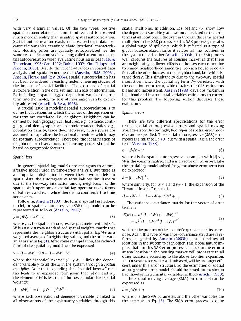
Table 1AFacilities in sample – MLB and MLB/NFL/NHL.

Facility name Sport Team MSA/CMSA

Chase Field/Bank One Ballpark* MLB Diamondbacks Phoenix, AZ MSATurner Field* MLB Braves Atlanta, GA MSAOriole Park at Camden Yards* MLB Oriloes Baltimore, MD MSAFenway Park MLB Red Sox Boston–Lawrence–Salem, MA-NH CMSAWrigley Field MLB Cubs Chicago–Gary–Lake County, IL-IN-WI CMSANew Comiskey Park* MLB White Sox Chicago–Gary–Lake County, IL-IN-WI CMSAComiskey Park# MLB White Sox Chicago–Gary–Lake County, IL-IN-WI CMSAJacobs Field* MLB Indians Cleveland–Akron–Lorain, OH CMSACoors Field* MLB Rockies Denver–Boulder, CO CMSAComericaPark* MLB Tigers Detroit–Ann Arbor, MI CMSATiger Stadium MLB Tigers Detroit–Ann Arbor, MI CMSAAstros Field* MLB Astros Houston–Galveston–Brazoria, TX CMSAKauffman Stadium MLB Royals Kansas City, MO-KS MSADodger Stadium MLB Dodgers Los Angeles–Anaheim–Riverside, CA CMSAMilwaukee County Stadium MLB Brewers Milwaukee–Racine, WI CMSAShea Stadium MLB Mets New York CMSAYankee Stadium MLB Yankees New York CMSAAT&TPark* MLB Giants San Francisco-Oakland-San Jose, CA CMSASafeCO Field* MLB Mariners Seattle–Tacoma, WA CMSABusch Stadium MLB Cardinals St. Louis, MO-IL MSABallpark at Arlington* MLB Rangers Dallas–Fort Worth, TX CMSAArlington Stadium# MLB Rangers Dallas–Fort Worth, TX CMSAAnaheim Stadium/Edison Field MLB/NFL Angels/Rams Los Angeles–Anaheim–Riverside, CA CMSAAtlanta–Fulton County Stadium# MLB/NFL Braves/Falcons Atlanta, GA MSABaltimore Memorial Stadium MLB/NFL Orioles/Colts Baltimore, MD MSACleveland stadium# MLB/NFL Indians/Browns Cleveland–Akron–Lorain, OH CMSARiverfront Stadium/Cinergy Field MLB/NFL Reds/Bengals Cincinnati–Hamilton, OH-KY-IN CMSAMile High Stadium MLB/NFL Rockies/Broncos Denver–Boulder, CO CMSADolphin Stadium MLB/NFL Marins/ Miami Dolphins Miami–Fort Lauderdale, FL CMSAAstrodome MLB/NFL Astros/Oilers Houston–Galveston–Brazoria, TX CMSAOakland Coliseum MLB/NFL Athletics/Raiders San Francisco–Oakland–San Jose, CA CMSAVeterans Stadium MLB/NFL Phillies/Eagles Philadelphia CMSAThree Rivers Stadium MLB/NFL Pirates/Steelers Pittsburgh–Beaver Valley, PA CMSAQualcomm Stadium MLB/NFL Padres/Chargers San Diego, CA MSACandlestick Park MLB/NFL Giants/49ers San Francisco–Oakland–San Jose, CA CMSAKingdome# MLB/NFL Mariners/Seahawks Seattle–Tacoma, WA CMSAMetrodome MLB/NFL/NBA Twins/Vikings/T-wolves Minneapolis–St. Paul, MN–WI MSATropicana Field* MLB/NHL Devil Rays/Lightning Tampa–St. Petersburg–Clearwater, FL MSA

4 For 1990, we only include those facilities built before 1990 and not demolished by1990. The stadiums with * were built after 1990 and therefore not included in the1990 sample but in the 2000 sample. For the 2000 sample, we only include those builtbefore (including) 2000 and not demolished by 2000. The stadiums with # weredemolished by 2000 and therefore not included in the 2000 sample but are still in the1990 sample.

194 X. Feng, B.R. Humphreys / City, Culture and Society 3 (2012) 189–200

tion represents a compromise between the MSA level dataused by Carlino and Coulson (2004) and Kiel et al. (2010),and the micro-level data used by Tu (2005), Dehring, et al(2007) and Ahlfeld and Maennig (2010), Kiel et al. (2010)and Ahlfeldt and Kavetsos (2011). Census block groupsare collections of census blocks containing between 600and 3000 people. They are the smallest unit of analysis inpublicly available Census data that contain both demo-graphic and economic characteristics and geographicaldescriptors that will allow us to correct for spatial depen-dence. Data at more aggregated levels, like counties orMSAs would obscure the spatial effects, while publiclyavailable Census micro data do not contain detailed geo-graphic descriptors. The main limitation of block groupdata is that the block group median or average values donot fully reflect the underlying distributions of propertyvalues in the micro data. But we feel that the benefits ofusing data at the block-group level, in terms of providingdata from a large number of metropolitan areas acrossthe country and a large number of sports facilities, out-weighs the limitations.

We use block group level data from the 1990 and 2000Censuses. Unfortunately, we cannot pool these data be-cause the geographical boundaries of the block groupschanged from 1990 to 2000. Thus for any particular 1990Census block group, there does not exist an exact corre-sponding block group in the 2000 Census. Because of this

lack of correspondence, we estimate separate models forthe 1990 and 2000 Censuses.

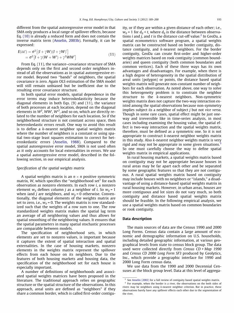
Our data contain all of the stadiums and arenas in use inthe NFL, NBA, NHL, and MLB in the 1990 and/or 2000 Cen-sus. This comprehensive set of sports facilities yields a largedata set containing 126 individual sports facilities in 45MSAs. Tables 1A, 1B and 1C show the facilities includedin the sample, the MSAs, and the teams that play in them.4

Table 2 contains summary statistics for the key variablesappearing in Eq. (3), the spatial hedonic model. The samplecontains 28,500 block groups in 1990 and 30,346 blockgroups in 2000. The dependent variable is the median valueof all owner occupied housing units in each block group.The average of these block group medians in the samplewas $116,131 in 1990 and $162,228 in 2000. For the hous-ing structure attributes, the mean value of percent of owneroccupied units with complete kitchen facilities and withplumbing facilities is close to 100% for both periods. Mostof the sports facility sites in the sample contained multiplefacilities.

Table 1BFacilities in sample, NBA and NBA/NHL.

Facility name Sport Team MSA/CMSA

Charlotte Coliseum NBA Hornets Charlotte–Gastonia–Rock Hill, NC–SC MSAQuicken Loans Arena* NBA Cavaliers Cleveland–Akron–Lorain, OH CMSARichfield Coliseum# NBA Cavaliers Cleveland–Akron–Lorain, OH CMSAMcNichols Sports Arena# NBA Nuggets Denver–Boulder, CO CMSACobo Arena NBA Pistons Detroit–Ann Arbor, MI CMSAThe Palace of Auburn Hills NBA Pistons Detroit–Ann Arbor, MI CMSAOakland Arena NBA Warriors San Francisco–Oakland–San Jose, CA CMSAThe CompaqCenter NBA Rockets Houston–Galveston–Brazoria, TX CMSAConseco Fieldhouse* NBA Pacers Indianapolis, IN MSAMarket Square Arena NBA Pacers Indianapolis, IN MSAThe Los Angeles Sports Arena NBA Clippers Los Angeles–Anaheim–Riverside, CA CMSAMemphis Pyramid* NBA Grizzlies Memphis, TN-MS-AR MSAAmerican Airlines Arena* NBA Heat Miami–Fort Lauderdale, FL CMSAThe Bradley Center NBA Bucks Milwaukee–Racine, WI CMSATarget Center NBA Timberwolves Minneapolis–St. Paul, MN–WI MSANew Orleans Arena* NBA Hornets New Orleans, LA MSATD Waterhouse Centre NBA Magic Orlando, FL MSARose Graden* NBA Trailblazers Portland–Vancouver, OR–WA CMSAThe Memorial Coliseum NBA Trailblazers Portland–Vancouver, OR–WA CMSAThe Arco Arena NBA Kings Sacramento, CA MSAAlamodome* NBA Spurs San Antonio, TX MSAHemisFair Arena# NBA Spurs San Antonio, TX MSAKey Arena NBA Supersonics Seattle–Tacoma, WA CMSADeltaCenter* NBA Jazz Salt Lake City–Ogden, UT MSASpectrum NBA/NHL 76ers/Flyers Philadelphia CMSAThe Omni# NBA/NHL Hawks /Flames Atlanta, GA MSAPhilips Arena* NBA/NHL Hawks/ Thrashers Atlanta, GA MSATD Banknorth Garden* NBA/NHL Celtics/Bruins Boston–Lawrence–Salem, MA-NH CMSAThe Boston Garden# NBA/NHL Celtics/Bruins Boston–Lawrence–Salem, MA-NH CMSAUnited Center* NBA/NHL Bulls/ Blackhawks Chicago–Gary–Lake County, IL–IN–WI CMSAChicago Stadium# NBA/NHL Bulls/Blackhawks Chicago–Gary–Lake County, IL–IN–WI CMSAReunion Arena NBA/NHL Mavericks/Stars Dallas–Fort Worth, TX CMSAPepsi Center* NBA/NHL Nuggets/ Avalanche Denver–Boulder, CO CMSAStaples Center* NBA/NHL Lakers/Clippers/ Kings Los Angeles–Anaheim–Riverside, CA CMSAGreat Western Forum NBA/NHL Lakers/Kings Los Angeles–Anaheim–Riverside, CA CMSAThe Miami Arena NBA/NHL Heat/Panthers Miami–Fort Lauderdale, FL CMSAMilwaukee Arena NBA Bucks Milwaukee–Racine, WI CMSAContinental Airlines Arena NBA/NHL Nets/ Devils New York CMSAMadison Square Garden NBA/NHL Knicks/Rangers New York CMSAFirst Union Center* NBA/NHL 76ers/ Flyers Philadelphia CMSAAmerica West Arena* NBA/NHL Suns/Coyotes Phoenix, AZ MSAVerizon Center* NBA/NHL Bullets/ Capitals Washington, DC-MD-VA MSACapital Center NBA/NHL Wizards/Capitals Washington, DC-MD-VA MSA

X. Feng, B.R. Humphreys / City, Culture and Society 3 (2012) 189–200 195

One of the major issues in the hedonic housing literatureis the selection of control variables to explain observed var-iation in housing values. The literature contains two broadcategories of explanatory variables: characteristics of thehousing units, including lot size and structural characteris-tics; and characteristics of the neighborhood, including so-cio-economic characteristics such as racial compositionand median household income, and public amenities suchas schools and parks. The latter category is the focus ofmany hedonic studies and has been extended to includecrime, air quality, water quality, and other environmentalamenities.5 Ideally, the empirical model should control foras many housing unit specific and neighborhood specificcharacteristics as possible, but sometimes data availabilityis a major determinant of the selection of explanatoryvariables.

We use explanatory variables, grouped into three cate-gories: housing structure attributes, neighborhood charac-teristics, and sports facility related characteristics. Thefirst category contains percent of owner occupied housing

5 See Boyle and Kiel (2001) for a full review of house price hedonic studies. Butsome studies did not include any neighborhood characteristics at all (Basu &Thibodeau, 1998; Can, 1992).

units with structure detached, average number of bed-rooms in owner occupied housing units, average numberof vehicles owned by owner occupied housing units, andmedian age of owner occupied housing units. Most of thesehousing attributes are examined in the standard hedonichousing literature but the selection of these housing attri-butes is influenced by data availability.

The second category, neighborhood characteristics,seems to be unmotivated in the hedonic literature. Thesevariables are often included in an ad hoc fashion, with littletheoretical justification foundation and empirical motiva-tion. Following the existing literature and some theoreticalconsiderations, our choices in the second category includemedian block group household income, distance from theblock group to the central business district (CBD),6 percentof population 25 years old and over with high school orequivalent degrees, percent of population 25 years old andover with bachelor’s degrees, percent of population that isblack, and percent of Hispanic population. In addition we in-clude a vector of city specific dummy variables to capture

6 All the distance variables are calculated from centroid to centroid of the blockgroups. For example, distance to the CBD is calculated from the centroid of each blockgroup to the centroid of CBD block groups. Distance to the sports facility is calculatedfrom the centroid of each block group to the block group where the facility is located.

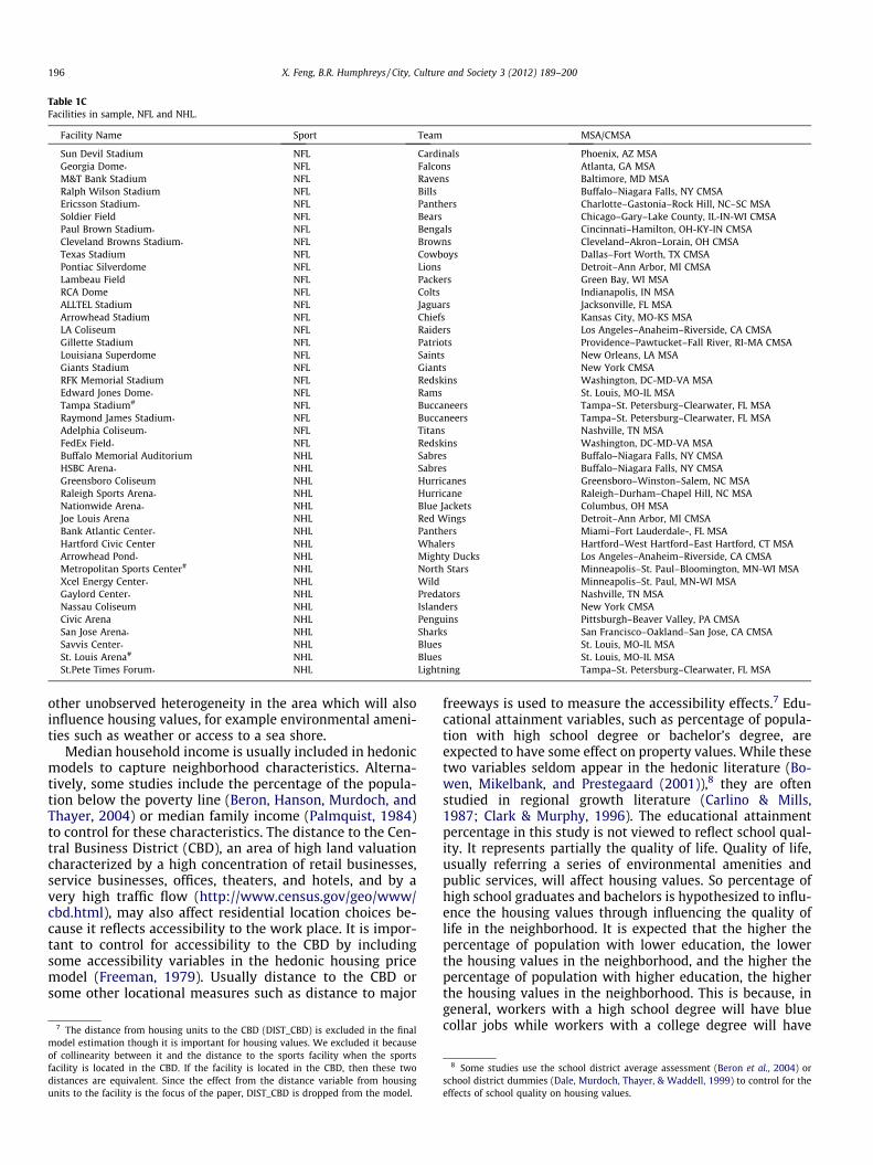
Table 1CFacilities in sample, NFL and NHL.

Facility Name Sport Team MSA/CMSA

Sun Devil Stadium NFL Cardinals Phoenix, AZ MSAGeorgia Dome* NFL Falcons Atlanta, GA MSAM&T Bank Stadium NFL Ravens Baltimore, MD MSARalph Wilson Stadium NFL Bills Buffalo–Niagara Falls, NY CMSAEricsson Stadium* NFL Panthers Charlotte–Gastonia–Rock Hill, NC–SC MSASoldier Field NFL Bears Chicago–Gary–Lake County, IL-IN-WI CMSAPaul Brown Stadium* NFL Bengals Cincinnati–Hamilton, OH-KY-IN CMSACleveland Browns Stadium* NFL Browns Cleveland–Akron–Lorain, OH CMSATexas Stadium NFL Cowboys Dallas–Fort Worth, TX CMSAPontiac Silverdome NFL Lions Detroit–Ann Arbor, MI CMSALambeau Field NFL Packers Green Bay, WI MSARCA Dome NFL Colts Indianapolis, IN MSAALLTEL Stadium NFL Jaguars Jacksonville, FL MSAArrowhead Stadium NFL Chiefs Kansas City, MO-KS MSALA Coliseum NFL Raiders Los Angeles–Anaheim–Riverside, CA CMSAGillette Stadium NFL Patriots Providence–Pawtucket–Fall River, RI-MA CMSALouisiana Superdome NFL Saints New Orleans, LA MSAGiants Stadium NFL Giants New York CMSARFK Memorial Stadium NFL Redskins Washington, DC-MD-VA MSAEdward Jones Dome* NFL Rams St. Louis, MO-IL MSATampa Stadium# NFL Buccaneers Tampa–St. Petersburg–Clearwater, FL MSARaymond James Stadium* NFL Buccaneers Tampa–St. Petersburg–Clearwater, FL MSAAdelphia Coliseum* NFL Titans Nashville, TN MSAFedEx Field* NFL Redskins Washington, DC-MD-VA MSABuffalo Memorial Auditorium NHL Sabres Buffalo–Niagara Falls, NY CMSAHSBC Arena* NHL Sabres Buffalo–Niagara Falls, NY CMSAGreensboro Coliseum NHL Hurricanes Greensboro–Winston–Salem, NC MSARaleigh Sports Arena* NHL Hurricane Raleigh–Durham–Chapel Hill, NC MSANationwide Arena* NHL Blue Jackets Columbus, OH MSAJoe Louis Arena NHL Red Wings Detroit–Ann Arbor, MI CMSABank Atlantic Center* NHL Panthers Miami–Fort Lauderdale-, FL MSAHartford Civic Center NHL Whalers Hartford–West Hartford–East Hartford, CT MSAArrowhead Pond* NHL Mighty Ducks Los Angeles–Anaheim–Riverside, CA CMSAMetropolitan Sports Center# NHL North Stars Minneapolis–St. Paul–Bloomington, MN-WI MSAXcel Energy Center* NHL Wild Minneapolis–St. Paul, MN-WI MSAGaylord Center* NHL Predators Nashville, TN MSANassau Coliseum NHL Islanders New York CMSACivic Arena NHL Penguins Pittsburgh–Beaver Valley, PA CMSASan Jose Arena* NHL Sharks San Francisco–Oakland–San Jose, CA CMSASavvis Center* NHL Blues St. Louis, MO-IL MSASt. Louis Arena# NHL Blues St. Louis, MO-IL MSASt.Pete Times Forum* NHL Lightning Tampa–St. Petersburg–Clearwater, FL MSA

196 X. Feng, B.R. Humphreys / City, Culture and Society 3 (2012) 189–200

other unobserved heterogeneity in the area which will alsoinfluence housing values, for example environmental ameni-ties such as weather or access to a sea shore.

Median household income is usually included in hedonicmodels to capture neighborhood characteristics. Alterna-tively, some studies include the percentage of the popula-tion below the poverty line (Beron, Hanson, Murdoch, andThayer, 2004) or median family income (Palmquist, 1984)to control for these characteristics. The distance to the Cen-tral Business District (CBD), an area of high land valuationcharacterized by a high concentration of retail businesses,service businesses, offices, theaters, and hotels, and by avery high traffic flow (http://www.census.gov/geo/www/cbd.html), may also affect residential location choices be-cause it reflects accessibility to the work place. It is impor-tant to control for accessibility to the CBD by includingsome accessibility variables in the hedonic housing pricemodel (Freeman, 1979). Usually distance to the CBD orsome other locational measures such as distance to major

7 The distance from housing units to the CBD (DIST_CBD) is excluded in the finalmodel estimation though it is important for housing values. We excluded it becauseof collinearity between it and the distance to the sports facility when the sportsfacility is located in the CBD. If the facility is located in the CBD, then these twodistances are equivalent. Since the effect from the distance variable from housingunits to the facility is the focus of the paper, DIST_CBD is dropped from the model.

freeways is used to measure the accessibility effects.7 Edu-cational attainment variables, such as percentage of popula-tion with high school degree or bachelor’s degree, areexpected to have some effect on property values. While thesetwo variables seldom appear in the hedonic literature (Bo-wen, Mikelbank, and Prestegaard (2001)),8 they are oftenstudied in regional growth literature (Carlino & Mills,1987; Clark & Murphy, 1996). The educational attainmentpercentage in this study is not viewed to reflect school qual-ity. It represents partially the quality of life. Quality of life,usually referring a series of environmental amenities andpublic services, will affect housing values. So percentage ofhigh school graduates and bachelors is hypothesized to influ-ence the housing values through influencing the quality oflife in the neighborhood. It is expected that the higher thepercentage of population with lower education, the lowerthe housing values in the neighborhood, and the higher thepercentage of population with higher education, the higherthe housing values in the neighborhood. This is because, ingeneral, workers with a high school degree will have bluecollar jobs while workers with a college degree will have

8 Some studies use the school district average assessment (Beron et al., 2004) orschool district dummies (Dale, Murdoch, Thayer, & Waddell, 1999) to control for theeffects of school quality on housing values.

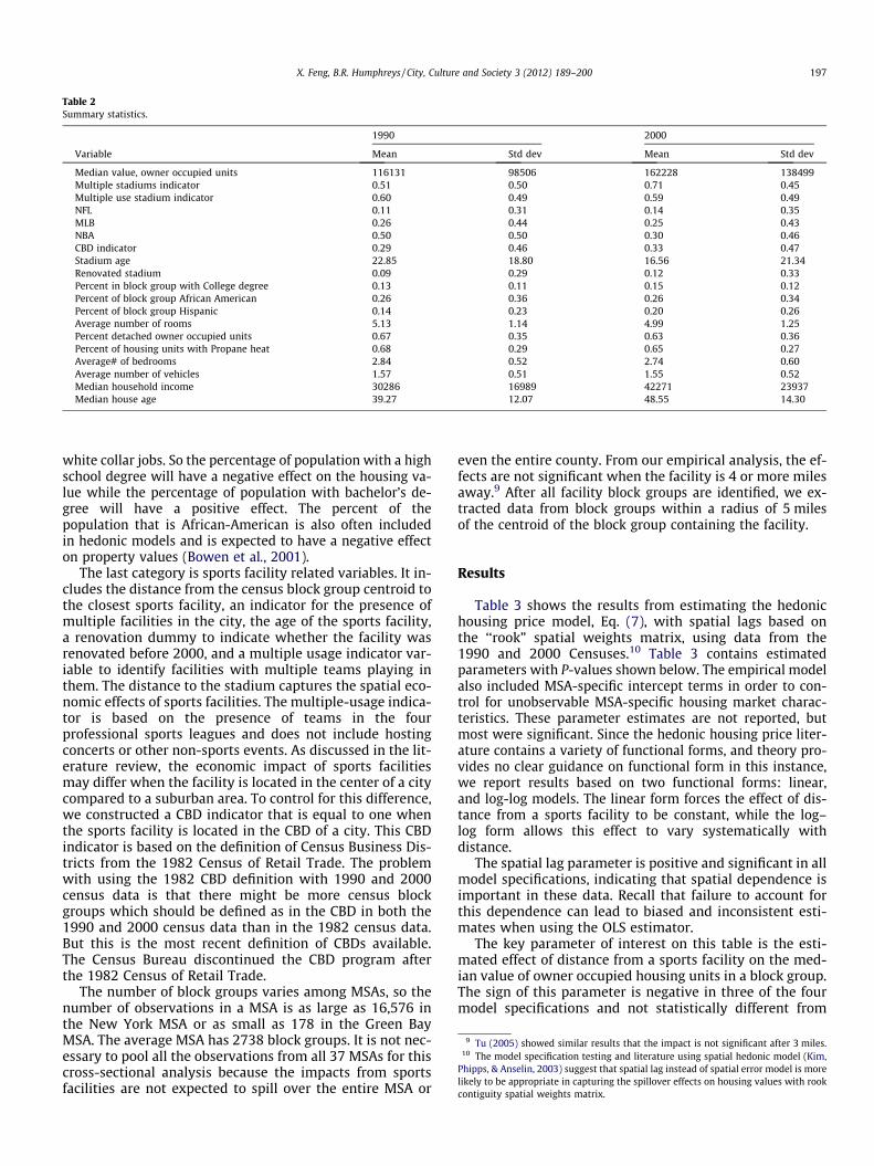
Table 2Summary statistics.

1990 2000

Variable Mean Std dev Mean Std dev

Median value, owner occupied units 116131 98506 162228 138499Multiple stadiums indicator 0.51 0.50 0.71 0.45Multiple use stadium indicator 0.60 0.49 0.59 0.49NFL 0.11 0.31 0.14 0.35MLB 0.26 0.44 0.25 0.43NBA 0.50 0.50 0.30 0.46CBD indicator 0.29 0.46 0.33 0.47Stadium age 22.85 18.80 16.56 21.34Renovated stadium 0.09 0.29 0.12 0.33Percent in block group with College degree 0.13 0.11 0.15 0.12Percent of block group African American 0.26 0.36 0.26 0.34Percent of block group Hispanic 0.14 0.23 0.20 0.26Average number of rooms 5.13 1.14 4.99 1.25Percent detached owner occupied units 0.67 0.35 0.63 0.36Percent of housing units with Propane heat 0.68 0.29 0.65 0.27Average# of bedrooms 2.84 0.52 2.74 0.60Average number of vehicles 1.57 0.51 1.55 0.52Median household income 30286 16989 42271 23937Median house age 39.27 12.07 48.55 14.30

9 Tu (2005) showed similar results that the impact is not significant after 3 miles.10 The model specification testing and literature using spatial hedonic model (Kim,

Phipps, & Anselin, 2003) suggest that spatial lag instead of spatial error model is morelikely to be appropriate in capturing the spillover effects on housing values with rookcontiguity spatial weights matrix.

X. Feng, B.R. Humphreys / City, Culture and Society 3 (2012) 189–200 197

white collar jobs. So the percentage of population with a highschool degree will have a negative effect on the housing va-lue while the percentage of population with bachelor’s de-gree will have a positive effect. The percent of thepopulation that is African-American is also often includedin hedonic models and is expected to have a negative effecton property values (Bowen et al., 2001).

The last category is sports facility related variables. It in-cludes the distance from the census block group centroid tothe closest sports facility, an indicator for the presence ofmultiple facilities in the city, the age of the sports facility,a renovation dummy to indicate whether the facility wasrenovated before 2000, and a multiple usage indicator var-iable to identify facilities with multiple teams playing inthem. The distance to the stadium captures the spatial eco-nomic effects of sports facilities. The multiple-usage indica-tor is based on the presence of teams in the fourprofessional sports leagues and does not include hostingconcerts or other non-sports events. As discussed in the lit-erature review, the economic impact of sports facilitiesmay differ when the facility is located in the center of a citycompared to a suburban area. To control for this difference,we constructed a CBD indicator that is equal to one whenthe sports facility is located in the CBD of a city. This CBDindicator is based on the definition of Census Business Dis-tricts from the 1982 Census of Retail Trade. The problemwith using the 1982 CBD definition with 1990 and 2000census data is that there might be more census blockgroups which should be defined as in the CBD in both the1990 and 2000 census data than in the 1982 census data.But this is the most recent definition of CBDs available.The Census Bureau discontinued the CBD program afterthe 1982 Census of Retail Trade.

The number of block groups varies among MSAs, so thenumber of observations in a MSA is as large as 16,576 inthe New York MSA or as small as 178 in the Green BayMSA. The average MSA has 2738 block groups. It is not nec-essary to pool all the observations from all 37 MSAs for thiscross-sectional analysis because the impacts from sportsfacilities are not expected to spill over the entire MSA or

even the entire county. From our empirical analysis, the ef-fects are not significant when the facility is 4 or more milesaway.9 After all facility block groups are identified, we ex-tracted data from block groups within a radius of 5 milesof the centroid of the block group containing the facility.

Results

Table 3 shows the results from estimating the hedonichousing price model, Eq. (7), with spatial lags based onthe ‘‘rook” spatial weights matrix, using data from the1990 and 2000 Censuses.10 Table 3 contains estimatedparameters with P-values shown below. The empirical modelalso included MSA-specific intercept terms in order to con-trol for unobservable MSA-specific housing market charac-teristics. These parameter estimates are not reported, butmost were significant. Since the hedonic housing price liter-ature contains a variety of functional forms, and theory pro-vides no clear guidance on functional form in this instance,we report results based on two functional forms: linear,and log-log models. The linear form forces the effect of dis-tance from a sports facility to be constant, while the log–log form allows this effect to vary systematically withdistance.

The spatial lag parameter is positive and significant in allmodel specifications, indicating that spatial dependence isimportant in these data. Recall that failure to account forthis dependence can lead to biased and inconsistent esti-mates when using the OLS estimator.

The key parameter of interest on this table is the esti-mated effect of distance from a sports facility on the med-ian value of owner occupied housing units in a block group.The sign of this parameter is negative in three of the fourmodel specifications and not statistically different from

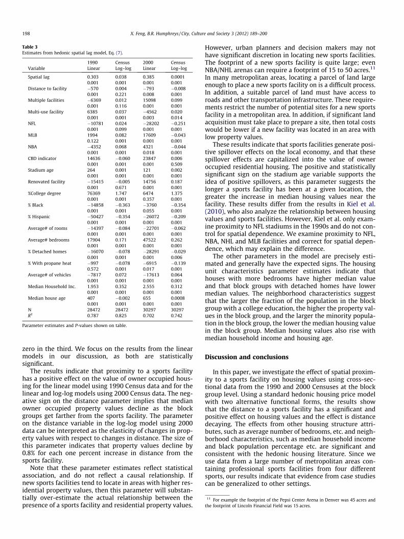
Table 3Estimates from hedonic spatial lag model, Eq. (7).

1990 Census 2000 CensusVariable Linear Log–log Linear Log–log

Spatial lag 0.303 0.038 0.385 0.00010.001 0.001 0.001 0.001

Distance to facility �570 0.004 �793 �0.0080.001 0.221 0.008 0.001

Multiple facilities �6369 0.012 15098 0.0990.001 0.116 0.001 0.001

Multi-use facility 6385 0.037 �4562 0.0200.001 0.001 0.003 0.014

NFL �10781 0.024 �28202 �0.2510.001 0.099 0.001 0.001

MLB 1994 0.082 17609 �0.0430.122 0.001 0.001 0.001

NBA �4352 0.068 4321 �0.0440.001 0.001 0.018 0.001

CBD indicator 14636 �0.060 23847 0.0060.001 0.001 0.001 0.509

Stadium age 264 0.001 121 0.0020.001 0.001 0.001 0.001

Renovated facility �15415 �0.005 14756 0.1870.001 0.671 0.001 0.001

%College degree 76369 1.747 6474 1.3750.001 0.001 0.357 0.001

% Black �14858 �0.363 �3760 �0.3540.001 0.001 0.055 0.001

% Hispanic �50427 �0.354 �26072 �0.2090.001 0.001 0.001 0.001

Average# of rooms �14397 �0.084 �22701 �0.0620.001 0.001 0.001 0.001

Average# bedrooms 17904 0.171 47522 0.2620.001 0.001 0.001 0.001

% Detached homes �16070 �0.078 �28291 �0.0290.001 0.001 0.001 0.006

% With propane heat �997 �0.078 �6915 �0.1390.572 0.001 0.017 0.001

Average# of vehicles �7817 0.072 �17613 0.0640.001 0.001 0.001 0.001

Median Household Inc. 1.953 0.352 2.555 0.3120.001 0.001 0.001 0.001

Median house age 407 �0.002 655 0.00080.001 0.001 0.001 0.001

N 28472 28472 30297 30297R2 0.787 0.825 0.702 0.742

Parameter estimates and P-values shown on table.

11 For example the footprint of the Pepsi Center Arena in Denver was 45 acres andthe footprint of Lincoln Financial Field was 15 acres.

198 X. Feng, B.R. Humphreys / City, Culture and Society 3 (2012) 189–200

zero in the third. We focus on the results from the linearmodels in our discussion, as both are statisticallysignificant.

The results indicate that proximity to a sports facilityhas a positive effect on the value of owner occupied hous-ing for the linear model using 1990 Census data and for thelinear and log-log models using 2000 Census data. The neg-ative sign on the distance parameter implies that medianowner occupied property values decline as the blockgroups get farther from the sports facility. The parameteron the distance variable in the log-log model using 2000data can be interpreted as the elasticity of changes in prop-erty values with respect to changes in distance. The size ofthis parameter indicates that property values decline by0.8% for each one percent increase in distance from thesports facility.

Note that these parameter estimates reflect statisticalassociation, and do not reflect a causal relationship. Ifnew sports facilities tend to locate in areas with higher res-idential property values, then this parameter will substan-tially over-estimate the actual relationship between thepresence of a sports facility and residential property values.

However, urban planners and decision makers may nothave significant discretion in locating new sports facilities.The footprint of a new sports facility is quite large; evenNBA/NHL arenas can require a footprint of 15 to 50 acres.11

In many metropolitan areas, locating a parcel of land largeenough to place a new sports facility on is a difficult process.In addition, a suitable parcel of land must have access toroads and other transportation infrastructure. These require-ments restrict the number of potential sites for a new sportsfacility in a metropolitan area. In addition, if significant landacquisition must take place to prepare a site, then total costswould be lower if a new facility was located in an area withlow property values.

These results indicate that sports facilities generate posi-tive spillover effects on the local economy, and that thesespillover effects are capitalized into the value of owneroccupied residential housing. The positive and statisticallysignificant sign on the stadium age variable supports theidea of positive spillovers, as this parameter suggests thelonger a sports facility has been at a given location, thegreater the increase in median housing values near thefacility. These results differ from the results in Kiel et al.(2010), who also analyze the relationship between housingvalues and sports facilities. However, Kiel et al. only exam-ine proximity to NFL stadiums in the 1990s and do not con-trol for spatial dependence. We examine proximity to NFL,NBA, NHL and MLB facilities and correct for spatial depen-dence, which may explain the difference.

The other parameters in the model are precisely esti-mated and generally have the expected signs. The housingunit characteristics parameter estimates indicate thathouses with more bedrooms have higher median valueand that block groups with detached homes have lowermedian values. The neighborhood characteristics suggestthat the larger the fraction of the population in the blockgroup with a college education, the higher the property val-ues in the block group, and the larger the minority popula-tion in the block group, the lower the median housing valuein the block group. Median housing values also rise withmedian household income and housing age.

Discussion and conclusions

In this paper, we investigate the effect of spatial proxim-ity to a sports facility on housing values using cross-sec-tional data from the 1990 and 2000 Censuses at the blockgroup level. Using a standard hedonic housing price modelwith two alternative functional forms, the results showthat the distance to a sports facility has a significant andpositive effect on housing values and the effect is distancedecaying. The effects from other housing structure attri-butes, such as average number of bedrooms, etc. and neigh-borhood characteristics, such as median household incomeand black population percentage etc. are significant andconsistent with the hedonic housing literature. Since weuse data from a large number of metropolitan areas con-taining professional sports facilities from four differentsports, our results indicate that evidence from case studiescan be generalized to other settings.

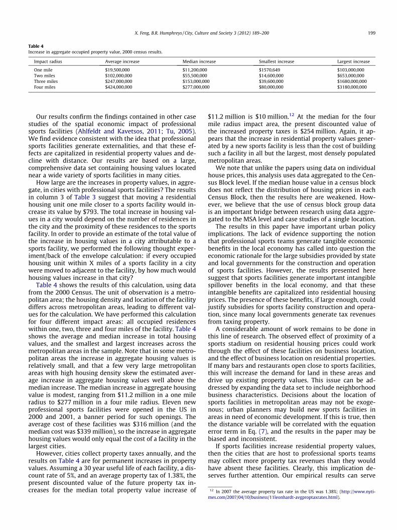
Table 4Increase in aggregate occupied property value, 2000 census results.

Impact radius Average increase Median increase Smallest increase Largest increase

One mile $19,500,000 $11,200,000 $1570,649 $103,000,000Two miles $102,000,000 $55,500,000 $14,600,000 $653,000,000Three miles $247,000,000 $153,000,000 $39,600,000 $1680,000,000Four miles $424,000,000 $277,000,000 $80,000,000 $3180,000,000

12 In 2007 the average property tax rate in the US was 1.38%; (http://www.nyti-

X. Feng, B.R. Humphreys / City, Culture and Society 3 (2012) 189–200 199

Our results confirm the findings contained in other casestudies of the spatial economic impact of professionalsports facilities (Ahlfeldt and Kavetsos, 2011; Tu, 2005).We find evidence consistent with the idea that professionalsports facilities generate externalities, and that these ef-fects are capitalized in residential property values and de-cline with distance. Our results are based on a large,comprehensive data set containing housing values locatednear a wide variety of sports facilities in many cities.

How large are the increases in property values, in aggre-gate, in cities with professional sports facilities? The resultsin column 3 of Table 3 suggest that moving a residentialhousing unit one mile closer to a sports facility would in-crease its value by $793. The total increase in housing val-ues in a city would depend on the number of residences inthe city and the proximity of these residences to the sportsfacility. In order to provide an estimate of the total value ofthe increase in housing values in a city attributable to asports facility, we performed the following thought exper-iment/back of the envelope calculation: if every occupiedhousing unit within X miles of a sports facility in a citywere moved to adjacent to the facility, by how much wouldhousing values increase in that city?

Table 4 shows the results of this calculation, using datafrom the 2000 Census. The unit of observation is a metro-politan area; the housing density and location of the facilitydiffers across metropolitan areas, leading to different val-ues for the calculation. We have performed this calculationfor four different impact areas: all occupied residenceswithin one, two, three and four miles of the facility. Table 4shows the average and median increase in total housingvalues, and the smallest and largest increases across themetropolitan areas in the sample. Note that in some metro-politan areas the increase in aggregate housing values isrelatively small, and that a few very large metropolitanareas with high housing density skew the estimated aver-age increase in aggregate housing values well above themedian increase. The median increase in aggregate housingvalue is modest, ranging from $11.2 million in a one mileradius to $277 million in a four mile radius. Eleven newprofessional sports facilities were opened in the US in2000 and 2001, a banner period for such openings. Theaverage cost of these facilities was $316 million (and themedian cost was $339 million), so the increase in aggregatehousing values would only equal the cost of a facility in thelargest cities.

However, cities collect property taxes annually, and theresults on Table 4 are for permanent increases in propertyvalues. Assuming a 30 year useful life of each facility, a dis-count rate of 5%, and an average property tax of 1.38%, thepresent discounted value of the future property tax in-creases for the median total property value increase of

$11.2 million is $10 million.12 At the median for the fourmile radius impact area, the present discounted value ofthe increased property taxes is $254 million. Again, it ap-pears that the increase in residential property values gener-ated by a new sports facility is less than the cost of buildingsuch a facility in all but the largest, most densely populatedmetropolitan areas.

We note that unlike the papers using data on individualhouse prices, this analysis uses data aggregated to the Cen-sus Block level. If the median house value in a census blockdoes not reflect the distribution of housing prices in eachCensus Block, then the results here are weakened. How-ever, we believe that the use of census block group datais an important bridge between research using data aggre-gated to the MSA level and case studies of a single location.

The results in this paper have important urban policyimplications. The lack of evidence supporting the notionthat professional sports teams generate tangible economicbenefits in the local economy has called into question theeconomic rationale for the large subsidies provided by stateand local governments for the construction and operationof sports facilities. However, the results presented heresuggest that sports facilities generate important intangiblespillover benefits in the local economy, and that theseintangible benefits are capitalized into residential housingprices. The presence of these benefits, if large enough, couldjustify subsidies for sports facility construction and opera-tion, since many local governments generate tax revenuesfrom taxing property.

A considerable amount of work remains to be done inthis line of research. The observed effect of proximity of asports stadium on residential housing prices could workthrough the effect of these facilities on business location,and the effect of business location on residential properties.If many bars and restaurants open close to sports facilities,this will increase the demand for land in these areas anddrive up existing property values. This issue can be ad-dressed by expanding the data set to include neighborhoodbusiness characteristics. Decisions about the location ofsports facilities in metropolitan areas may not be exoge-nous; urban planners may build new sports facilities inareas in need of economic development. If this is true, thenthe distance variable will be correlated with the equationerror term in Eq. (7), and the results in the paper may bebiased and inconsistent.

If sports facilities increase residential property values,then the cities that are host to professional sports teamsmay collect more property tax revenues than they wouldhave absent these facilities. Clearly, this implication de-serves further attention. Our empirical results can serve

mes.com/2007/04/10/business/11leonhardt-avgproptaxrates.html).

200 X. Feng, B.R. Humphreys / City, Culture and Society 3 (2012) 189–200

as the basis of a cost-benefit study comparing the value ofsports facility subsidies to the additional property tax rev-enues generated by these facilities.

Acknowledgements

We thank Luc Anselin, John Braden, Andy Isserman andparticipants in several REAP seminars at the University ofIllinois for valuable comments and suggestions.

References

Ahlfeld, G., & Maennig, W. (2010). Impact of sports arenas on land values: evidencefrom Berlin. Annals of Regional Science, 44(2), 205–227.

Ahlfeldt, G. M., & Kavetsos, G. (2011). Form or Function? The Impact of New FootballStadia on Property Prices in London, SERC Discussion Papers, Spatial EconomicsResearch Centre, LSE. http://EconPapers.repec.org/RePEc:cep:sercdp:0087.

Anselin, L. (1988). Spatial econometrics: methods and models. Boston: KluwerAcademic.

Anselin, L. (2002). Under the hood: issues in the specification and interpretation ofspatial regression models. Agricultural Economics, 27, 247–267.

Anselin, L. (2003a) GeoDa.Anselin, L. (2003). Spatial externalities, spatial multipliers, and spatial

econometrics. International Regional Science Review, 26(2), 153–166.Anselin, L., and Bera, A.K. (1998), ‘‘Spatial Dependence in Linear Regression Models

with an Introduction to Spatial Econometrics”, Handbook of Applied EconomicStatistics, Eds A. Ullah and D. Giles, New York: Marcel Dehker.

Anselin, L., Florax, R. J. G. M., & Rey, S. J. (Eds.). (2004). Advances in spatialeconometrics: methodology, tools and applications. Berlin: Springer-Verlag.

Basu, S., & Thibodeau, T. G. (1998). Analysis of spatial autocorrelation in houseprices. Journal of Real Estate Finance and Economics, 17(1), 61–85.

Beron, K.J., Hanson, Y., Murdoch, J.C., and Thayer, M.A. (2004), ‘‘Hedonic PriceFunctions and Spatial Dependence: Implications for the Demand for Urban AirQuality”, Chapter 12 in Advances in Spatial Econometrics: Methodology, Toolsand Applications. Berlin: Springer-Verlag .

Bowen, W. M., Mikelbank, B., & Prestegaard, D. M. (2001). Theoretical and empiricalconsiderations regarding space in hedonic housing price model applications.Growth and Change, 32(4).

Boyle, M. A., & Kiel, K. A. (2001). A survey of house price hedonic studies of theimpact of environmental externalities. Journal of Real Estate Literature, 19(2),116–144.

Can, A. (1992). Specification and estimation of hedonic housing price models.Regional Science and Urban Economics, 22(3), 453–474.

Carlino, G. A., & Coulson, N. E. (2004). Compensating differentials and the socialbenefits of the NFL. Journal of Urban Economics, 56(1), 25–50.

Carlino, G. A., & Mills, E. S. (1987). The determinants of county growth. Journal ofRegional Science, 27(1), 39–54.

Clark, D. E., & Murphy, C. A. (1996). Countywide employment and populationgrowth: an analysis of1980s. Journal of Regional Science, 36(2), 235–256.

Coates, D., & Humphreys, B. R. (2005). Proximity benefits and voting on stadium andarena subsidies. Journal of Urban Economics, 59(2), 285–299.

Dale, L., Murdoch, J. C., Thayer, M. A., & Waddell, P. A. (1999). Do property valuesrebound from environmental stigmas? Evidence from Dallas. Land Economics,75(2), 311–326.

Dehring, C. A., Depken, C. A., & Ward, M. R. (2007). The impact of stadiumannouncements on residential property values: evidence from a naturalexperiment in Dallas-fort worth. Contemporary Economic Policy, 25(4), 627–638.

Dubin, Robin A. (1992). Spatial autocorrelation and neighborhood quality. RegionalScience and Urban Economics, 22(3), 433–452.

Freeman, A. M. (1979). Hedonic prices, property values and measuringenvironmental benefits: a survey of the issues. Scandinavian Journal ofEconomics, 81(2), 154–173.

Kiel, K. A., Matheson, V. and Sullivan, C. (2010). ‘‘The Effect of Sports Franchises onProperty Values: The Role of Owners versus Renters,” Working Papers 1007,International Association of Sports Economists & North American Association ofSports Economists.

Kim, C. W., Phipps, T. T., & Anselin, L. (2003). Measuring the benefits of air qualityimprovement: a spatial hedonic approach. Journal of Environmental Economicsand Management, 45(1), 24–39.

Palmquist, R. B. (1984). Estimating the demand for the characteristics of housing.The Review of Economics and Statistics, 66(3), 394–404.

Tu, C. C. (2005). How does a new sports stadium affect housing values? The case ofFedEx field. Land Economics, 81(3), 379–395.