Classroom Tips and Techniques: Circle Inscribed in a Parabola

Robert J. Lopez

Emeritus Professor of Mathematics and Maple Fellow

Maplesoft

Introduction

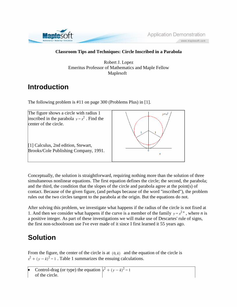
The following problem is #11 on page 300 (Problems Plus) in [1].

The figure shows a circle with radius 1

inscribed in the parabola . Find the

center of the circle.

[1] Calculus, 2nd edition, Stewart,

Brooks/Cole Publishing Company, 1991.

Conceptually, the solution is straightforward, requiring nothing more than the solution of three

simultaneous nonlinear equations. The first equation defines the circle; the second, the parabola;

and the third, the condition that the slopes of the circle and parabola agree at the point(s) of

contact. Because of the given figure, (and perhaps because of the word "inscribed"), the problem

rules out the two circles tangent to the parabola at the origin. But the equations do not.

After solving this problem, we investigate what happens if the radius of the circle is not fixed at

1. And then we consider what happens if the curve is a member of the family , where n is

a positive integer. As part of these investigations we will make use of Descartes' rule of signs,

the first non-schoolroom use I've ever made of it since I first learned it 55 years ago.

Solution

From the figure, the center of the circle is at and the equation of the circle is

. Table 1 summarizes the ensuing calculations.

Control-drag (or type) the equation

of the circle.

Press the Enter key.

Context Menu:

Differentiate≻Implicitly

Set y as the dependent variable; x as

the independent.

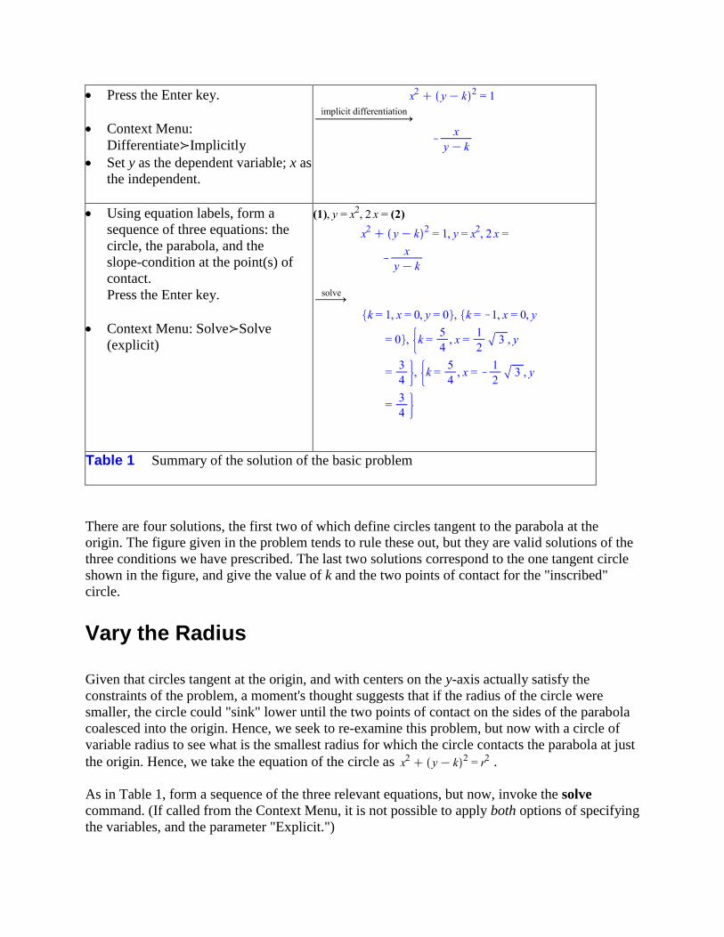
Using equation labels, form a

sequence of three equations: the

circle, the parabola, and the

slope-condition at the point(s) of

contact.

Press the Enter key.

Context Menu: Solve≻Solve

(explicit)

Table 1 Summary of the solution of the basic problem

There are four solutions, the first two of which define circles tangent to the parabola at the

origin. The figure given in the problem tends to rule these out, but they are valid solutions of the

three conditions we have prescribed. The last two solutions correspond to the one tangent circle

shown in the figure, and give the value of k and the two points of contact for the "inscribed"

circle.

Vary the Radius

Given that circles tangent at the origin, and with centers on the y-axis actually satisfy the

constraints of the problem, a moment's thought suggests that if the radius of the circle were

smaller, the circle could "sink" lower until the two points of contact on the sides of the parabola

coalesced into the origin. Hence, we seek to re-examine this problem, but now with a circle of

variable radius to see what is the smallest radius for which the circle contacts the parabola at just

the origin. Hence, we take the equation of the circle as .

As in Table 1, form a sequence of the three relevant equations, but now, invoke the solve

command. (If called from the Context Menu, it is not possible to apply both options of specifying

the variables, and the parameter "Explicit.")

Again, there are four solutions, the first two of which correspond to circles tangent at the origin.

The second two solutions correspond to the single circle tangent to the "sides" of the parabola.

From these solutions, we see that , so defines the circle for which the two

points of contact coalesce into the origin. This circle then has its center at .

Vary the Curve

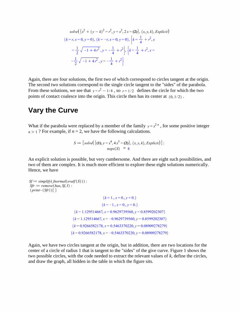
What if the parabola were replaced by a member of the family , for some positive integer

? For example, if n = 2, we have the following calculations.

=

An explicit solution is possible, but very cumbersome. And there are eight such possibilities, and

two of them are complex. It is much more efficient to explore these eight solutions numerically.

Hence, we have

Again, we have two circles tangent at the origin, but in addition, there are two locations for the

center of a circle of radius 1 that is tangent to the "sides" of the give curve. Figure 1 shows the

two possible circles, with the code needed to extract the relevant values of k, define the circles,

and draw the graph, all hidden in the table in which the figure sits.

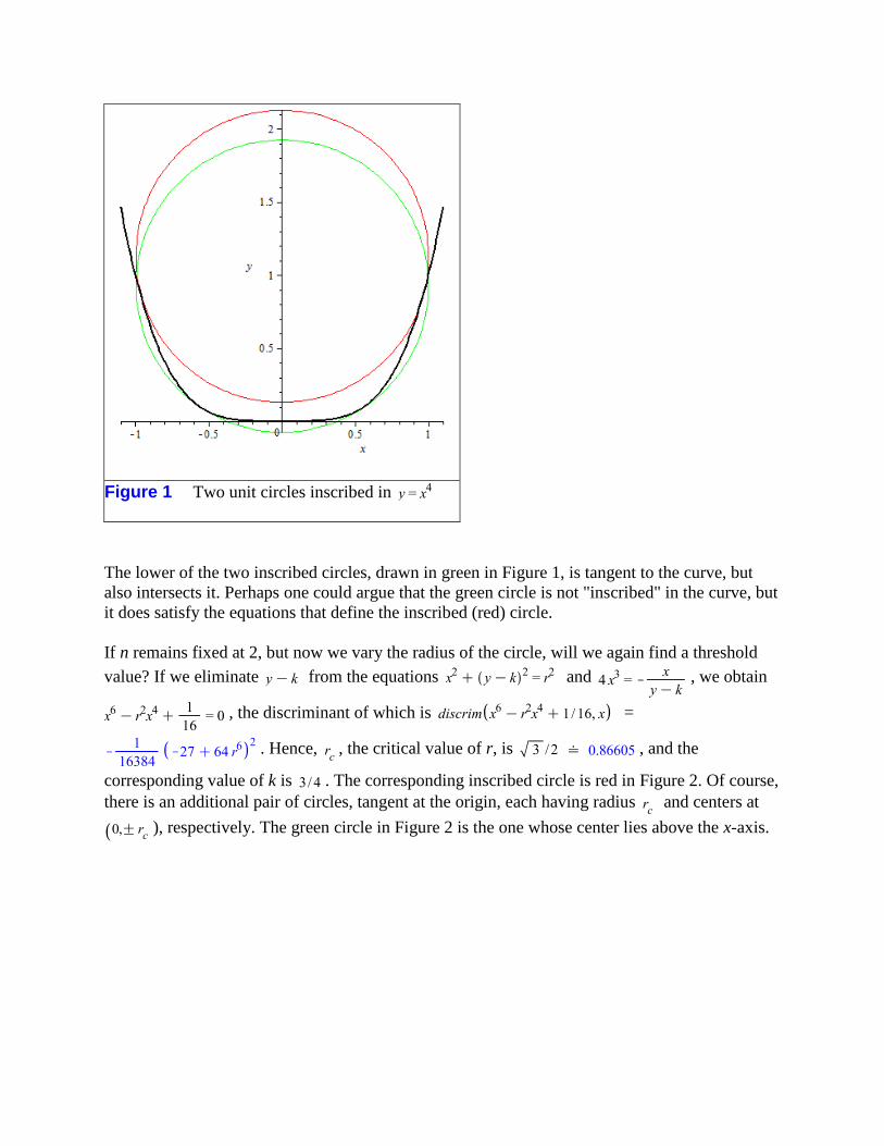
Figure 1 Two unit circles inscribed in

The lower of the two inscribed circles, drawn in green in Figure 1, is tangent to the curve, but

also intersects it. Perhaps one could argue that the green circle is not "inscribed" in the curve, but

it does satisfy the equations that define the inscribed (red) circle.

If n remains fixed at 2, but now we vary the radius of the circle, will we again find a threshold

value? If we eliminate from the equations and , we obtain

, the discriminant of which is =

. Hence, , the critical value of r, is , and the

corresponding value of k is . The corresponding inscribed circle is red in Figure 2. Of course,

there is an additional pair of circles, tangent at the origin, each having radius and centers at

), respectively. The green circle in Figure 2 is the one whose center lies above the x-axis.

Figure 2 One "inscribed" circle (red) when

=

The red circle in Figure 2 and the pair of circles tangent at the origin can be determined from the

real solutions of the equations

namely, from

If there are two circles inscribed in . Figure 1 exemplifies this case. If , there

is a pair of circles tangent at the origin, and with centers at .

Vary the Radius and the Curve

To what extent can we fathom the behavior of circles inscribed in the general member of the

family ? Some of the direct attacks we made above for the cases n = 1 and 2 fail for

general n. However, we can eliminate from the equations

, obtaining

We'd now like the discriminant of . Maple's discriminant for the polynomial p is obtained in

terms of the resultant of the polynomials p and its derivative. This resultant is a multiple of the

product of the evaluations of one polynomial at the zeros of the other. Since the zeros here are at

best expressed in terms of the RootOf structure, Maple's discrim command fails.

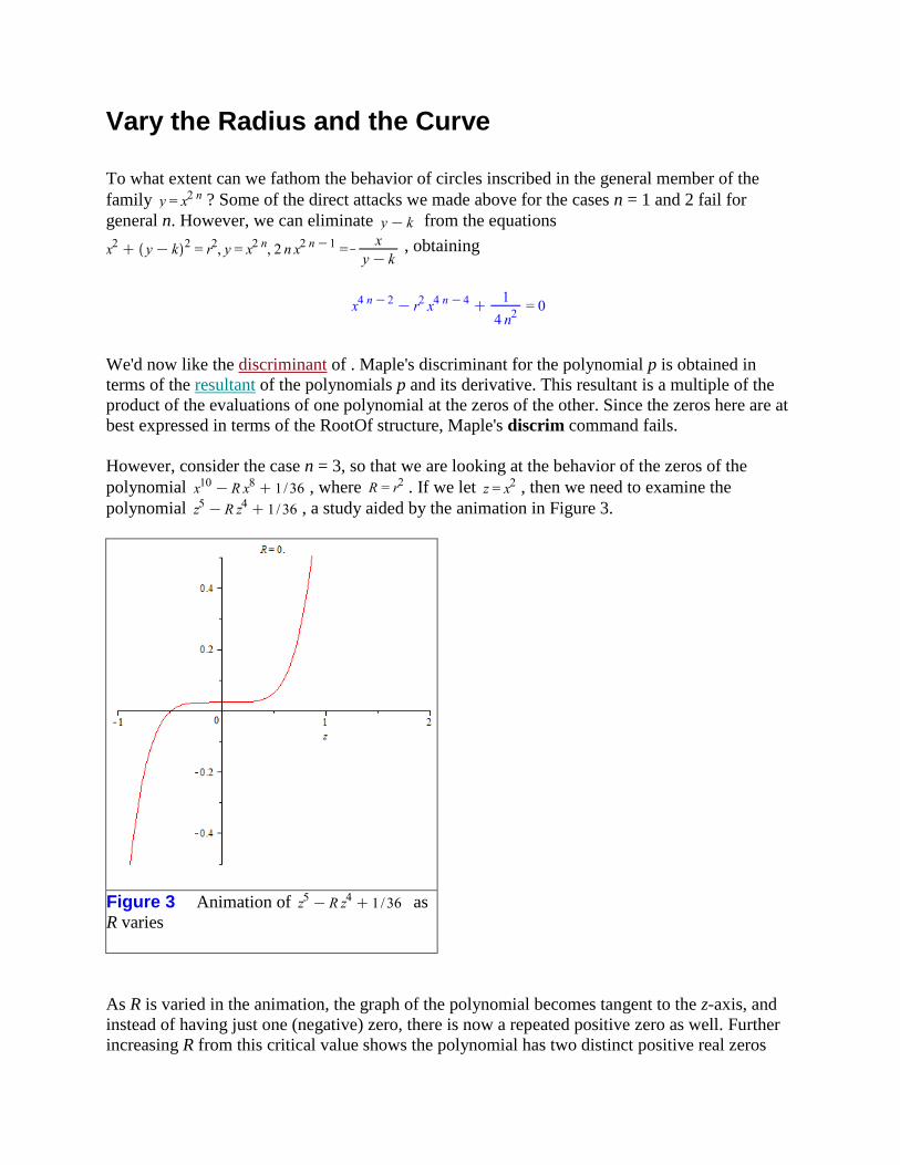
However, consider the case n = 3, so that we are looking at the behavior of the zeros of the

polynomial , where . If we let , then we need to examine the

polynomial , a study aided by the animation in Figure 3.

Figure 3 Animation of as

R varies

As R is varied in the animation, the graph of the polynomial becomes tangent to the z-axis, and

instead of having just one (negative) zero, there is now a repeated positive zero as well. Further

increasing R from this critical value shows the polynomial has two distinct positive real zeros

and still the one negative real zero. At the critical value of R, the polynomial has a zero at a zero

of derivative. That's why the discriminant is given in terms of the resultant, and why the resultant

is a product of the values of the polynomial at the zeros of the derivative.

In this particular case, when R causes the fifth-degree polynomial in z to have a repeated real,

positive zero, this zero is the value of , so taking the square root gives the positive and

negative values of the x-coordinate of the point of contact of the inscribed circle. And since x

appears as two even powers in , the substitution results in a polynomial equation

, where the polynomial is now of odd degree.

The zeros of this polynomial fall into one of three cases: one negative real zero, and (1) no

positive real zeros; and (2), a double positive real zero; and (3), two distinct positive real zeros.

We establish this with Descartes' rule of signs. There are two sign changes in the polynomial.

Hence, there are either two positive zeros, or no positive zeros. Changing z to its negative results

in a polynomial with one sign change, so there is exactly one negative real zero. Thus, as R

varies, there will be either no real positive zeros or two, and that includes the case of the double

real positive zero. (Incidentally, this is the only time since I got out of high school in 1958 that

I've ever made more than a pedantic use of Descartes' rule of signs. Shortly after starting college

came the computer age, and then came the calculator age, and who needed those cumbersome

processes for finding zeros of polynomials when there was all this wonderful technology

available?)

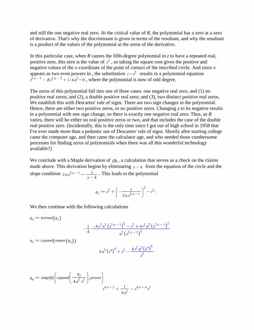
We conclude with a Maple derivation of , a calculation that serves as a check on the claims

made above. This derivation begins by eliminating from the equation of the circle and the

slope condition . This leads to the polynomial

We then continue with the following calculations

In essence, we have obtained . If we now differentiate and solve to find the critical number,

evaluate the polynomial at the critical number, set this expression equal to zero and solve for r,

we will have found , the critical value of the radius. Consequently, we continue with

as the critical number, and

as , the critical value of the radius as a function of n. Table 2 lists values for for several

values of n.

Table 2 Values of for several values of n

Legal Notice: © Maplesoft, a division of Waterloo Maple Inc. 2011. Maplesoft and Maple are

trademarks of Waterloo Maple Inc. This application may contain errors and Maplesoft is not

liable for any damages resulting from the use of this material. This application is intended for

non-commercial, non-profit use only. Contact Maplesoft for permission if you wish to use this

application in for-profit activities.