CLIMATE CHANGE MONITORING REPORT 2006

November 2007

JAPAN METEOROLOGICAL AGENCY

Published by the Japan Meteorological Agency

1-3-4 Otemachi, Chiyoda-ku, Tokyo 100-8122, Japan

Telephone +81 3 3211 4966 Facsimile +81 3 3211 2032 E-mail iao-jma@met.kishou.go.jp

CLIMATE CHANGE MONITORING REPORT 2006

November 2007

JAPAN METEOROLOGICAL AGENCY

Cover: Three-dimensional representations of monthly variations in zonally averaged atmospheric CO2 distribution (concentrations (top) and growth rates (bottom)). This analysis was performed using data archived by the WDCGG.

Preface There has been increasing global concern over the adverse effects that human activities have on the earth’s climate, and environmental issues such as global warming have become problems that need to be dealt with immediately worldwide. The Intergovernmental Panel on Climate Change (IPCC), established in 1988 by the World Meteorological Organization (WMO) and the United Nations Environment Programme (UNEP), indicated in its 4th Assessment Report adopted in February 2007 that warming of the climate system is unequivocal; the Scientific Assessment of Ozone Depletion report (WMO and UNEP et al (2006)) suggested that the Antarctic ozone hole is expected to continue for decades. In order to resolve these pressing issues of the global environment, it is necessary to comprehensively grasp the status and nature of the changes that are taking place in the climate system. This includes the atmosphere and oceans as well as atmospheric components such as carbon dioxide and ozone. The Japan Meteorological Agency (JMA), in close cooperation with the relevant national and international authorities and organizations including the WMO, has actively pursued monitoring of climate change and clarification of its mechanism. Since 1996, JMA has published a series of assessments under the title of Climate Change Monitoring Report. These publications include the outcome of JMA’s activities such as monitoring and analysis of greenhouse gases and the ozone layer, thereby providing up-to-date information on the climatic conditions of the world and Japan. The current issue reports several highlights from 2006 such as a record-high ozone hole size and the third-highest global average surface temperature in the last 120 years. Also included in this issue is new information on yellow sand (Aeolian dust), acid rain and oceanic pollution. It is my hope that readers of the report will find it useful in gaining a better understanding of the latest status of the climate toward further protection of the global environment. I would like to take this opportunity to convey my deep appreciation to the members of the Advisory Group of the Council for Climatic Issues of JMA under the chairmanship of Dr. H. Kondo for their pertinent comments and guidance in our work on this report.

(Tetsu Hiraki)

Director-General Japan Meteorological Agency

Contents

Part I Climate 1

1. Global climate 1.1 Global climate 1 1.2 Global surface temperature and precipitation 5

Column - Climate at Syowa Station, Antarctica 8 2. Climate of Japan

2.1 Climate of Japan in 2006 9 2.2 Major meteorological disasters in Japan 15

2.3 Surface temperature and precipitation in Japan 18 2.4 Long-term trend of extreme events in Japan 20 Column - Long-term trend of heavy rain analyzed from AMeDAS data 27

2.5 Tropical cyclones 30 2.6 Urban heat island effects in metropolitan areas of Japan 32

Part II Oceans 36

1. Global Oceans 1.1 Global sea surface temperature 36 1.2 El Niño and La Niña 38

1.3 Sea ice in the Arctic and Antarctic areas 42

2. The western North Pacific and the seas adjacent to Japan 2.1 Sea surface temperatures and ocean currents in the western North Pacific 43 2.2 Sea level around Japan 45

2.3 Sea ice in the Sea of Okhotsk 49 2.4 Marine pollution in the western North Pacific 50

Part III Atmospheric Environment 55

1. Monitoring of greenhouse gases and ozone-depleting substances 1.1 Greenhouse gases and ozone-depleting substances in the atmosphere 56 1.2 Oceanic carbon dioxide 67

1.3 Aerosols 71 2. Monitoring of the ozone layer and ultraviolet radiation

2.1 Observational results of the ozone layer 75 2.2 Solar UV radiation 79

3. Yellow sand (Aeolian dust) and acid rain 3.1 Yellow sand (Aeolian dust) 82 3.2 Acid rain 84

Map 1 Geographical subdivisions of Japan 86 Map 2 Distribution of surface meteorological observation stations in Japan 87

1

Part I Climate 1 Global climate

1.1 Global climate

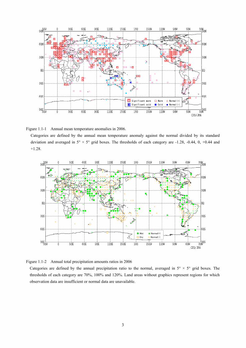
1.1.1 Major climate anomalies Figures 1.1-1 and 1.1-2 show anomalies in the annual mean temperature (normalized by its

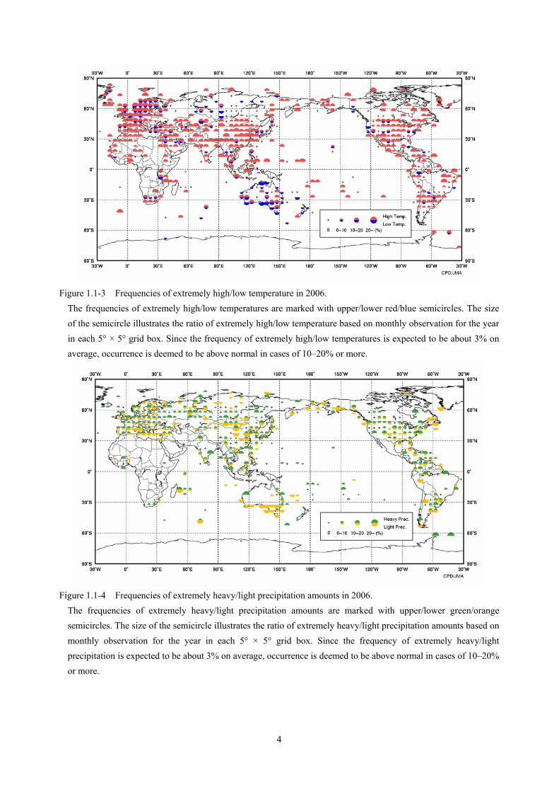
standard deviation) and ratios in the annual total precipitation amount in 2006 respectively. The climatological normal values for temperature and precipitation amounts are calculated using statistics from the period 1971–2000. Figures 1.1-3 and 1.1-4 show frequencies of extremely high/low temperatures and heavy/light precipitation amounts respectively. Extremely high/low temperatures and heavy/light precipitation amounts are defined as values that are observed only once every 30 years or longer. Monthly and seasonal values are omitted in this report.

Annual mean temperatures were above normal in most of the world except southern Siberia and the coastal areas of Australia. They were significantly higher in western Europe, eastern North America and from China to the Middle East (Figure 1.1-1). Extremely high temperatures were frequently observed over wide areas from Asia to Europe (Figure 1.1-3), especially in the latter half of the year, while extremely low temperatures were observed in Europe, Siberia and Australia for a few months.

Annual precipitation amounts were above normal in eastern and western Siberia, around India, southeastern Africa, around the Caribbean Sea and northwestern Australia, while they were below normal in southern Europe, southeastern Australia, over the eastern Indian Ocean and from Mongolia to northern China (Figure 1.1-2). Extremely heavy/light precipitation amounts were also frequently observed in the same areas (Figure 1.1-4). 1.1.2 Regional climate anomalies

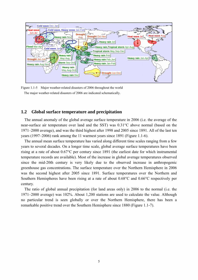
The regional climate anomalies of 2006 are described below. Major weather-related disasters reported by EM-DAT (the OFDA/CRED International Disaster Database of Belgium’s Université Catholique de Louvain) in 2006 are indicated schematically in Figure 1.1-5.

1) East Asia and Siberia

Annual temperatures were above normal except in southern Siberia. Extremely high monthly temperatures were frequently observed over wide areas of China in the latter half of the year. Annual precipitation amounts were above normal in eastern Siberia and from western Siberia to central Asia, while levels were below normal in Mongolia. Extremely light monthly precipitation amounts were frequently observed in northern China in spring and autumn, and in southwestern China in summer. It was extremely wet from Japan to the Korean peninsula due to the active Baiu front. 2) South Asia

Annual temperatures were above normal throughout the whole region, and extremely high monthly temperatures were frequently observed over wide areas. Annual precipitation amounts were above normal in the southern Philippines and from Pakistan to India, while they were

2

below normal in northeastern India. In southeastern Asia, extremely heavy monthly precipitation amounts were frequently observed in the northern part, while extremely light monthly precipitation amounts were observed in Indonesia in the latter half of the year. Around India, extremely heavy monthly precipitation amounts were frequently observed in Pakistan and western India. 3) Europe

Annual temperatures were above normal throughout the whole region, and extremely high monthly temperatures were frequently observed over wide areas of western Europe from April. In northern Europe, annual precipitation amounts were above normal, and extremely heavy monthly precipitation amounts were observed from autumn onward. In southern Europe, annual precipitation amounts were below normal, and extremely light monthly precipitation amounts were frequently observed from spring onward. 4) Africa and the Middle East

Annual temperatures were above normal in the regions for which monthly climate data are available. Extremely high monthly temperatures were observed over wide areas of northern Africa and the Middle East in June and August. Annual precipitation amounts were above normal in southeastern Africa, the islands of the western Indian Ocean and most of northwestern Africa, while they were below normal in a few parts of northwestern Africa and the Middle East. 5) North America

Annual temperatures were significantly higher except for northwestern North America. Extremely high monthly temperatures were observed over wide areas in January and April. Annual precipitation amounts were above normal from eastern Canada to the northeastern USA, from central Canada to the northwestern USA, from the southwestern USA to western Mexico and around the Caribbean Sea, while they were below normal in the central USA. It was extremely wet in the northeastern USA in June, September and October. 6) South America

Annual temperatures were above normal in the regions for which monthly climate data are available. Extremely high monthly temperatures were frequently observed. Annual precipitation amounts were above normal in Chile and around Venezuela, and extremely heavy monthly precipitation amounts were frequently observed around Venezuela in the first half of the year. 7) Oceania

Annual temperatures were above normal in the inner area of eastern Australia and from Micronesia to southern Polynesia. They were below normal in the coastal areas of Australia, and extremely low monthly temperatures were observed over wide areas of Australia in April and May. Annual precipitation amounts were above normal in northwestern Australia and northern Melanesia, while they were below normal in southeastern Australia and the islands of the eastern Indian Ocean. Extremely light precipitation amounts were observed in southeastern Australia in the latter half of the year.

3

Significant warm □ Warm ○ Normal(+)

Significant cold ■ Cold ● Normal(-)

Significant warm □ Warm ○ Normal(+)

Significant cold ■ Cold ● Normal(-)

Figure 1.1-1 Annual mean temperature anomalies in 2006.

Categories are defined by the annual mean temperature anomaly against the normal divided by its standard deviation and averaged in 5° × 5° grid boxes. The thresholds of each category are -1.28, -0.44, 0, +0.44 and +1.28.

● Wet ● Normal(+)

○ Dry ○ Normal(-)

Figure 1.1-2 Annual total precipitation amounts ratios in 2006

Categories are defined by the annual precipitation ratio to the normal, averaged in 5° × 5° grid boxes. The thresholds of each category are 70%, 100% and 120%. Land areas without graphics represent regions for which observation data are insufficient or normal data are unavailable.

4

Figure 1.1-3 Frequencies of extremely high/low temperature in 2006.

The frequencies of extremely high/low temperatures are marked with upper/lower red/blue semicircles. The size of the semicircle illustrates the ratio of extremely high/low temperature based on monthly observation for the year in each 5° × 5° grid box. Since the frequency of extremely high/low temperatures is expected to be about 3% on average, occurrence is deemed to be above normal in cases of 10–20% or more.

Figure 1.1-4 Frequencies of extremely heavy/light precipitation amounts in 2006.

The frequencies of extremely heavy/light precipitation amounts are marked with upper/lower green/orange semicircles. The size of the semicircle illustrates the ratio of extremely heavy/light precipitation amounts based on monthly observation for the year in each 5° × 5° grid box. Since the frequency of extremely heavy/light precipitation is expected to be about 3% on average, occurrence is deemed to be above normal in cases of 10–20% or more.

5

Heat waveJun-Jul

Heat waveHeat waveJun-Jul

Heavy rain JulHeavy rainHeavy rain Jul

Heavy rain Aug-NovHeavy rainHeavy rain Aug-Nov

Cold wave, Heavy snow Jan-FebCold wave, Heavy snowCold wave, Heavy snow Jan-Feb

Drought Jan-JunDroughtDrought Jan-Jun

Cold wave Dec-JanCold waveCold wave Dec-Jan

Heat wave JulHeat waveHeat wave Jul Heat wave AugHeat waveHeat wave Aug

Drought Jun-DecDroughtDrought Jun-Dec

Heavy rain NovHeavy rainHeavy rain Nov

Heavy rain FebHeavy rainHeavy rain Feb

Heavy rain Feb,JunHeavy rainHeavy rain Feb,Jun

Tropical storm May,Sep-DecTropical stormTropical storm May,Sep-Dec

Heavy rainMay,Aug-OctHeavy rainHeavy rain

May,Aug-Oct

DroughtAug

DroughtDroughtAug

Heavy rain Jan-AprHeavy rainHeavy rain Jan-Apr

Flood Mar-AprFloodFlood Mar-Apr

Heavy rain DecHeavy rainHeavy rain Dec

Heavy rainMay-Aug

Heavy rainHeavy rainMay-Aug

Storm Sep-OctSSttormorm Sep-Oct Heavy rain Jan-FebHeavy rainHeavy rain Jan-Feb

Cold wave JanCold waveCold wave Jan Heavy rain,Tropical storm Apr-AugHeavy Heavy rainrain,Tropical,Tropical stormstorm Apr-Aug

Drought Oct-NovDroughtDrought Oct-Nov

Figure 1.1-5 Major weather-related disasters of 2006 throughout the world

The major weather-related disasters of 2006 are indicated schematically.

1.2 Global surface temperature and precipitation

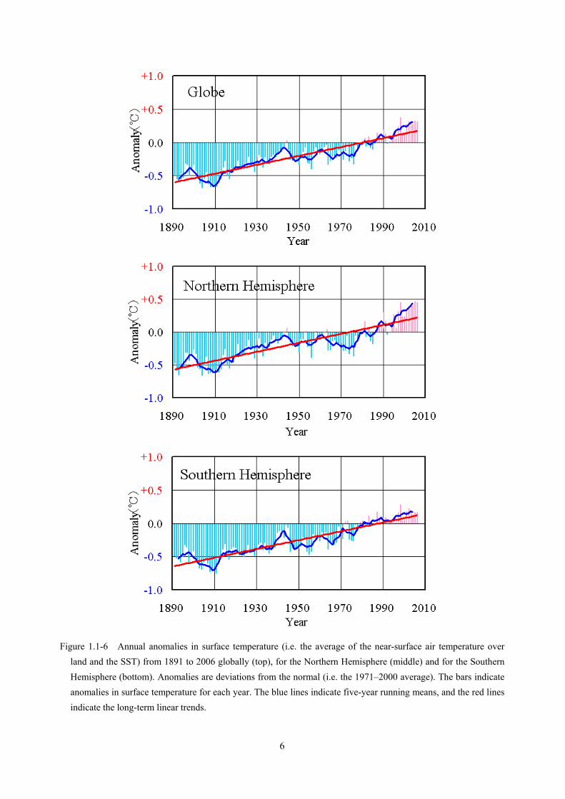
The annual anomaly of the global average surface temperature in 2006 (i.e. the average of the near-surface air temperature over land and the SST) was 0.31°C above normal (based on the 1971–2000 average), and was the third highest after 1998 and 2005 since 1891. All of the last ten years (1997–2006) rank among the 11 warmest years since 1891 (Figure 1.1-6).

The annual mean surface temperature has varied along different time scales ranging from a few years to several decades. On a longer time scale, global average surface temperatures have been rising at a rate of about 0.67°C per century since 1891 (the earliest date for which instrumental temperature records are available). Most of the increase in global average temperatures observed since the mid-20th century is very likely due to the observed increase in anthropogenic greenhouse gas concentrations. The surface temperature over the Northern Hemisphere in 2006 was the second highest after 2005 since 1891. Surface temperatures over the Northern and Southern Hemispheres have been rising at a rate of about 0.68°C and 0.66°C respectively per century.

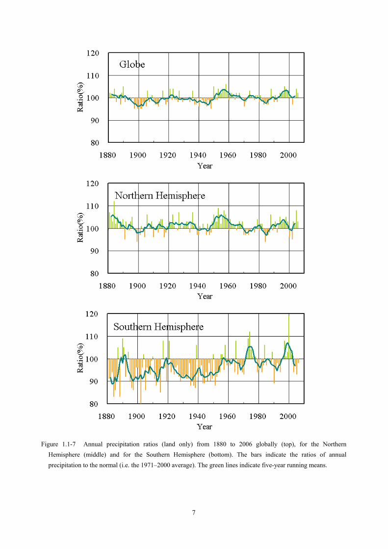
The ratio of global annual precipitation (for land areas only) in 2006 to the normal (i.e. the 1971–2000 average) was 102%. About 1,200 stations are used to calculate the value. Although no particular trend is seen globally or over the Northern Hemisphere, there has been a remarkable positive trend over the Southern Hemisphere since 1880 (Figure 1.1-7).

6

Figure 1.1-6 Annual anomalies in surface temperature (i.e. the average of the near-surface air temperature over

land and the SST) from 1891 to 2006 globally (top), for the Northern Hemisphere (middle) and for the Southern Hemisphere (bottom). Anomalies are deviations from the normal (i.e. the 1971–2000 average). The bars indicate anomalies in surface temperature for each year. The blue lines indicate five-year running means, and the red lines indicate the long-term linear trends.

7

Figure 1.1-7 Annual precipitation ratios (land only) from 1880 to 2006 globally (top), for the Northern Hemisphere (middle) and for the Southern Hemisphere (bottom). The bars indicate the ratios of annual precipitation to the normal (i.e. the 1971–2000 average). The green lines indicate five-year running means.

8

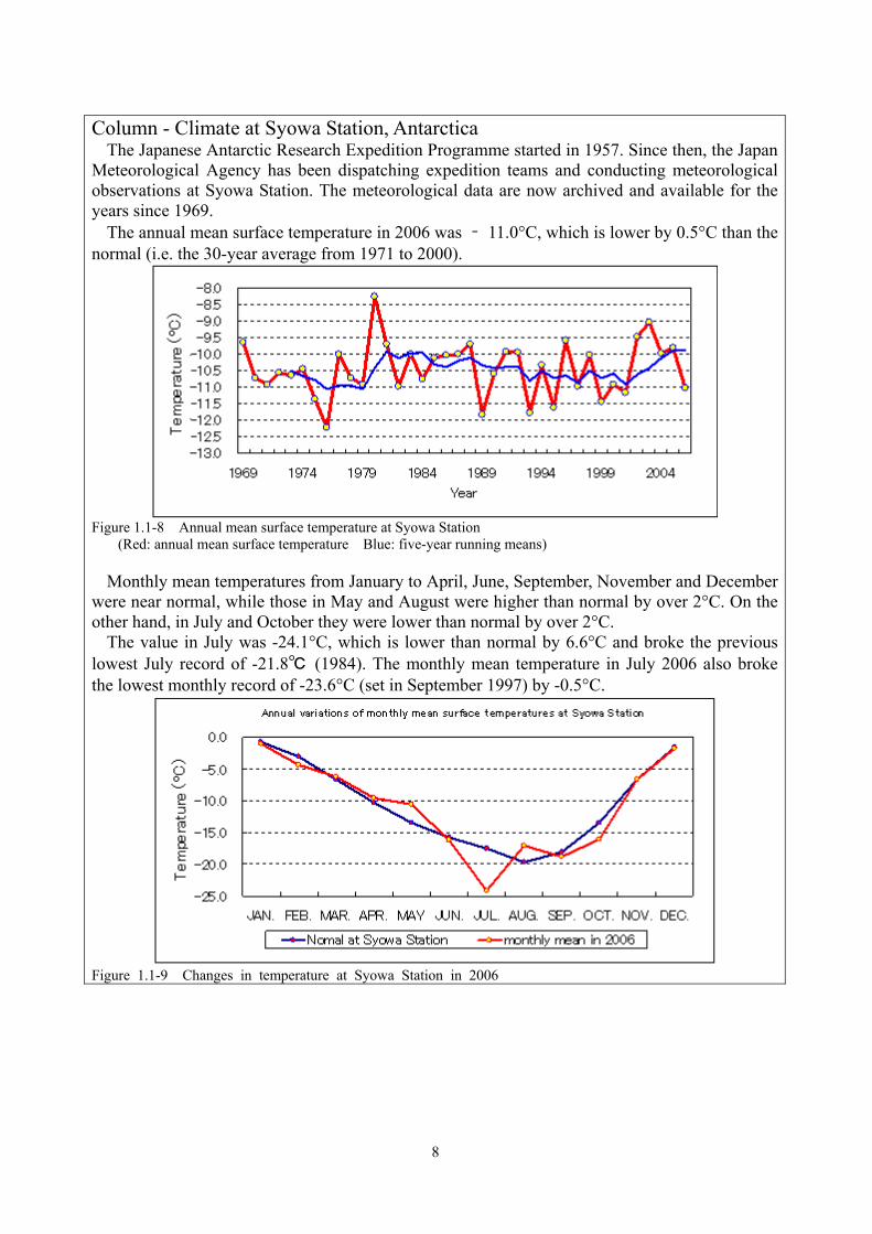
Column - Climate at Syowa Station, Antarctica The Japanese Antarctic Research Expedition Programme started in 1957. Since then, the Japan

Meteorological Agency has been dispatching expedition teams and conducting meteorological observations at Syowa Station. The meteorological data are now archived and available for the years since 1969.

The annual mean surface temperature in 2006 was – 11.0°C, which is lower by 0.5°C than the normal (i.e. the 30-year average from 1971 to 2000).

Figure 1.1-8 Annual mean surface temperature at Syowa Station

(Red: annual mean surface temperature Blue: five-year running means)

Monthly mean temperatures from January to April, June, September, November and December were near normal, while those in May and August were higher than normal by over 2°C. On the other hand, in July and October they were lower than normal by over 2°C.

The value in July was -24.1°C, which is lower than normal by 6.6°C and broke the previous lowest July record of -21.8℃ (1984). The monthly mean temperature in July 2006 also broke the lowest monthly record of -23.6°C (set in September 1997) by -0.5°C.

Figure 1.1-9 Changes in temperature at Syowa Station in 2006

9

2 Climate of Japan

2.1 Japan’s Climate in 2006

Through December 2005 and the first half of January 2006, strong winter monsoon patterns repeatedly appeared and brought record snowfall on the Japan Sea side for the first time in about two decades. In the latter half of the winter, warm days alternatively appeared, but sporadic heavy snowfall, avalanches and snow-related flooding occurred in mountainous areas. JMA refers to these conditions as “the heavy snowfall of winter 2006”.

In spring, fluctuations in temperature were large and spring mean temperatures were near normal in most regions of Japan. Cold vortices passing slowly over Japan in April and active stationary fronts along the Pacific coast in May brought unusually low sunshine durations in most regions.

The onset of the Baiu front (Japan’s rainy season) was near normal or later than normal in most regions of the country. The front was more active than in normal years, and heavy rainfall occurred nationwide. Remarkably heavy rainfall, referred to by JMA as “the heavy rainfall of July 2006”, continued from 15 to 24 July, and serious disasters were experienced nationwide. The end of the Baiu front was later than normal in most regions, except for an early departure in the Nansei Islands which resulted in below-normal sunshine durations in summer nationwide. In August, on the other hand, hot days were dominant due to the Pacific high covering Japan, and summer mean temperatures were above normal in all regions.

Warm, fine days were dominant nationwide in autumn due to frequent migratory highs and rare cold spells. Autumn mean temperatures were above normal, and the western and eastern parts of Japan experienced a record-breaking warm October. The Akisame front (which brings rainy days in autumn as the Baiu front does in early summer) was inactive, which resulted in above-normal sunshine durations nationwide and remarkably little rain in western Japan and the Nansei Islands. Conversely, in northern and eastern Japan, several developed lows brought heavy rainfall. In November, short-period deluges and tornadoes frequently occurred due to the unstable atmosphere forming low-level advection of wetter and warmer air. A tornado that hit Saroma Town in Hokkaido district caused serious damage.

Warm days were also dominant in December due to a weaker-than-normal winter monsoon, and snowfall amounts on the Japan Sea side were below normal.

The number of tropical cyclones (TC) with a maximum wind speed stronger than 17.2 m/s formed in the western North Pacific in 2006 was 23, which was below normal (normal: 26.7, range of near-normal: 25-29). The number of landfalls on the mainland of Japan was two, which was near normal (normal: 2.6). The number of TCs that came within 300 km of the mainland and islands of Japan was ten, which was also near normal (normal: 10.8). A tornado that formed in concurrence with Typhoon 0613 caused serious damage to Nobeoka City in Miyazaki Prefecture.

2.1.1 Annual climate anomalies and records (Table 1.2-1, Figure 1.2-1) 1) Annual mean temperatures

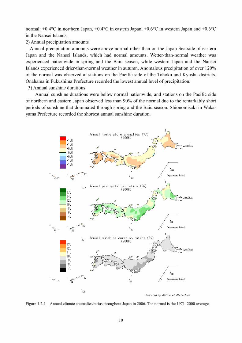
The anomaly of nationwide annual mean temperatures was +0.44°C, the tenth highest on record since 1898 (details in Section 2.3). Regional mean temperature anomalies were all above

10

normal: +0.4°C in northern Japan, +0.4°C in eastern Japan, +0.6°C in western Japan and +0.6°C in the Nansei Islands. 2) Annual precipitation amounts

Annual precipitation amounts were above normal other than on the Japan Sea side of eastern Japan and the Nansei Islands, which had normal amounts. Wetter-than-normal weather was experienced nationwide in spring and the Baiu season, while western Japan and the Nansei Islands experienced drier-than-normal weather in autumn. Anomalous precipitation of over 120% of the normal was observed at stations on the Pacific side of the Tohoku and Kyushu districts. Onahama in Fukushima Prefecture recorded the lowest annual level of precipitation. 3) Annual sunshine durations

Annual sunshine durations were below normal nationwide, and stations on the Pacific side of northern and eastern Japan observed less than 90% of the normal due to the remarkably short periods of sunshine that dominated through spring and the Baiu season. Shionomisaki in Waka-yama Prefecture recorded the shortest annual sunshine duration.

Figure 1.2-1 Annual climate anomalies/ratios throughout Japan in 2006. The normal is the 1971–2000 average.

11

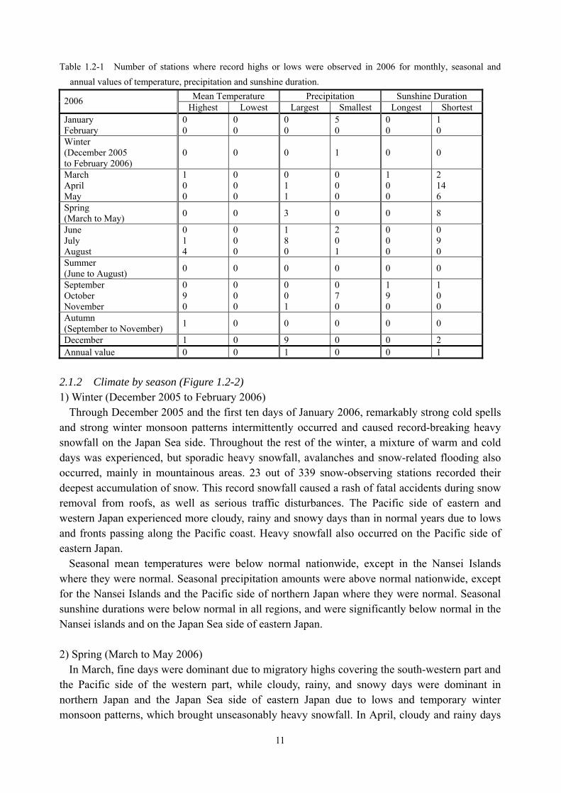
Table 1.2-1 Number of stations where record highs or lows were observed in 2006 for monthly, seasonal and annual values of temperature, precipitation and sunshine duration.

Mean Temperature Precipitation Sunshine Duration 2006 Highest Lowest Largest Smallest Longest Shortest

January February

0 0

0 0

0 0

5 0

0 0

1 0

Winter (December 2005 to February 2006)

0 0 0 1 0 0

March April May

1 0 0

0 0 0

0 1 1

0 0 0

1 0 0

2 14 6

Spring (March to May) 0 0 3 0 0 8

June July August

0 1 4

0 0 0

1 8 0

2 0 1

0 0 0

0 9 0

Summer (June to August) 0 0 0 0 0 0

September October November

0 9 0

0 0 0

0 0 1

0 7 0

1 9 0

1 0 0

Autumn (September to November) 1 0 0 0 0 0

December 1 0 9 0 0 2 Annual value 0 0 1 0 0 1

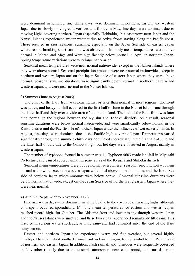
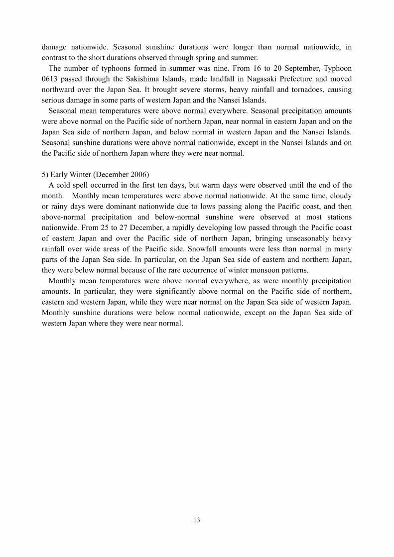
2.1.2 Climate by season (Figure 1.2-2) 1) Winter (December 2005 to February 2006)

Through December 2005 and the first ten days of January 2006, remarkably strong cold spells and strong winter monsoon patterns intermittently occurred and caused record-breaking heavy snowfall on the Japan Sea side. Throughout the rest of the winter, a mixture of warm and cold days was experienced, but sporadic heavy snowfall, avalanches and snow-related flooding also occurred, mainly in mountainous areas. 23 out of 339 snow-observing stations recorded their deepest accumulation of snow. This record snowfall caused a rash of fatal accidents during snow removal from roofs, as well as serious traffic disturbances. The Pacific side of eastern and western Japan experienced more cloudy, rainy and snowy days than in normal years due to lows and fronts passing along the Pacific coast. Heavy snowfall also occurred on the Pacific side of eastern Japan.

Seasonal mean temperatures were below normal nationwide, except in the Nansei Islands where they were normal. Seasonal precipitation amounts were above normal nationwide, except for the Nansei Islands and the Pacific side of northern Japan where they were normal. Seasonal sunshine durations were below normal in all regions, and were significantly below normal in the Nansei islands and on the Japan Sea side of eastern Japan. 2) Spring (March to May 2006)

In March, fine days were dominant due to migratory highs covering the south-western part and the Pacific side of the western part, while cloudy, rainy, and snowy days were dominant in northern Japan and the Japan Sea side of eastern Japan due to lows and temporary winter monsoon patterns, which brought unseasonably heavy snowfall. In April, cloudy and rainy days

12

were dominant nationwide, and chilly days were dominant in northern, eastern and western Japan due to slowly moving cold vortices and fronts. In May, fine days were dominant due to moving highs covering northern Japan (especially Hokkaido), but eastern/western Japan and the Nansei Islands experienced wetter weather due to active fronts staying along the Pacific coast. These resulted in short seasonal sunshine, especially on the Japan Sea side of eastern Japan where record-breaking short sunshine was observed. Monthly mean temperatures were above normal in March and May, and were significantly below normal in April in northern Japan. Spring temperature variations were very large nationwide.

Seasonal mean temperatures were near normal nationwide, except in the Nansei Islands where they were above normal. Seasonal precipitation amounts were near normal nationwide, except in northern and western Japan and on the Japan Sea side of eastern Japan where they were above normal. Seasonal sunshine durations were significantly below normal in northern, eastern and western Japan, and were near normal in the Nansei Islands. 3) Summer (June to August 2006)

The onset of the Baiu front was near normal or later than normal in most regions. The front was active, and heavy rainfall occurred in the first half of June in the Nansei Islands and through the latter half and July over a wide area of the main island. The end of the Baiu front was later than normal in the regions between the Kyushu and Tohoku districts. As a result, seasonal sunshine durations were below normal nationwide, and were significantly below normal in the Kanto district and the Pacific side of northern Japan under the influence of wet easterly winds. In August, fine days were dominant due to the Pacific high covering Japan. Temperatures varied significantly through the summer; chilly days dominated sporadically in the first half of June and the latter half of July due to the Okhotsk high, but hot days were observed in August mainly in western Japan.

The number of typhoons formed in summer was 11. Typhoon 0603 made landfall in Miyazaki Prefecture, and caused severe rainfall in some areas of the Kyushu and Shikoku districts.

Seasonal mean temperatures were above normal everywhere. Seasonal precipitation was near normal nationwide, except in western Japan which had above normal amounts, and the Japan Sea side of northern Japan where amounts were below normal. Seasonal sunshine durations were below normal nationwide, except on the Japan Sea side of northern and eastern Japan where they were near normal.

4) Autumn (September to November 2006)

Fine and warm days were dominant nationwide due to the coverage of moving highs, although cold spells occurred sporadically. Monthly mean temperatures for eastern and western Japan reached record highs for October. The Akisame front and lows passing through western Japan and the Nansei Islands were inactive, and these two areas experienced remarkably little rain. This resulted in serious water shortages, as little rainwater had remained since the end of the Baiu rainy season.

Eastern and northern Japan also experienced warm and fine weather, but several highly developed lows supplied southerly warm and wet air, bringing heavy rainfall to the Pacific side of northern and eastern Japan. In addition, flash rainfall and tornadoes were frequently observed in November (mainly due to the unstable atmosphere near cold fronts), and caused serious

13

damage nationwide. Seasonal sunshine durations were longer than normal nationwide, in contrast to the short durations observed through spring and summer.

The number of typhoons formed in summer was nine. From 16 to 20 September, Typhoon 0613 passed through the Sakishima Islands, made landfall in Nagasaki Prefecture and moved northward over the Japan Sea. It brought severe storms, heavy rainfall and tornadoes, causing serious damage in some parts of western Japan and the Nansei Islands.

Seasonal mean temperatures were above normal everywhere. Seasonal precipitation amounts were above normal on the Pacific side of northern Japan, near normal in eastern Japan and on the Japan Sea side of northern Japan, and below normal in western Japan and the Nansei Islands. Seasonal sunshine durations were above normal nationwide, except in the Nansei Islands and on the Pacific side of northern Japan where they were near normal. 5) Early Winter (December 2006)

A cold spell occurred in the first ten days, but warm days were observed until the end of the month. Monthly mean temperatures were above normal nationwide. At the same time, cloudy or rainy days were dominant nationwide due to lows passing along the Pacific coast, and then above-normal precipitation and below-normal sunshine were observed at most stations nationwide. From 25 to 27 December, a rapidly developing low passed through the Pacific coast of eastern Japan and over the Pacific side of northern Japan, bringing unseasonably heavy rainfall over wide areas of the Pacific side. Snowfall amounts were less than normal in many parts of the Japan Sea side. In particular, on the Japan Sea side of eastern and northern Japan, they were below normal because of the rare occurrence of winter monsoon patterns.

Monthly mean temperatures were above normal everywhere, as were monthly precipitation amounts. In particular, they were significantly above normal on the Pacific side of northern, eastern and western Japan, while they were near normal on the Japan Sea side of western Japan. Monthly sunshine durations were below normal nationwide, except on the Japan Sea side of western Japan where they were near normal.

14

(a) (b)

(c) (d)

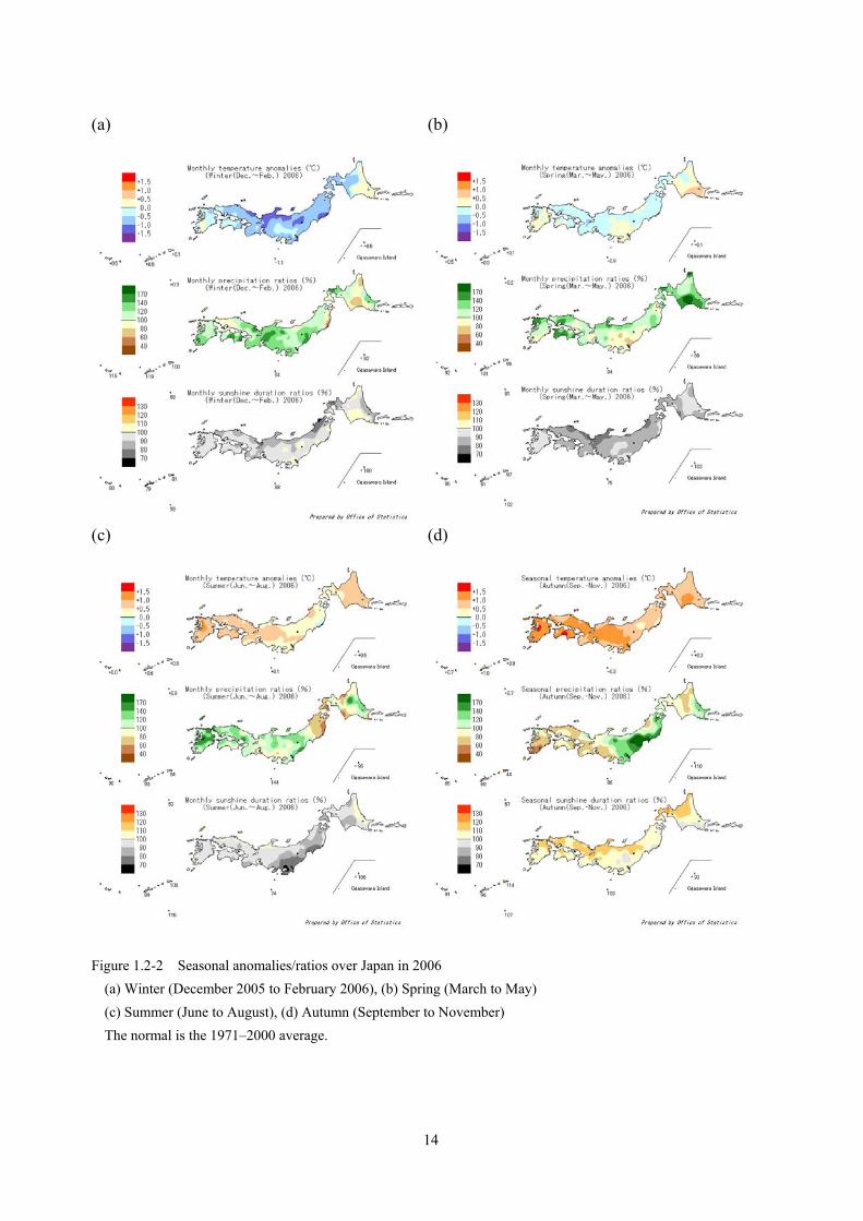
Figure 1.2-2 Seasonal anomalies/ratios over Japan in 2006

(a) Winter (December 2005 to February 2006), (b) Spring (March to May) (c) Summer (June to August), (d) Autumn (September to November) The normal is the 1971–2000 average.

15

2.2 Major meteorological disasters in Japan

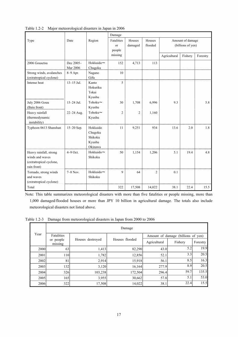
The meteorological disasters of 2006 were characterized by the 2006 Gousetsu (heavy snowfall) between December 2005 and March 2006, and the extensive tornado-related damage that accompanied the typhoon and rain front in Miyazaki Prefecture’s Nobeoka City and Hokkaido’s Saroma Town. In terms of the total damage caused by disasters in 2006, 322 people were killed or unaccounted for, 17,508 houses were damaged or destroyed, and 14,022 houses were flooded. The total damage amounted to 76.0 billion yen (details: 38.1 billion yen agricultural, 15.5 billion yen forestry and 22.4 billion yen fishery damages).

This section, including Table 1.2-2, summarizes the major meteorological disasters of 2006 and their causes.

Table 1.2-3 shows damage caused by meteorological disasters from 2000 to 2006.

Ｏ The 2006 Gousetsu (December 2005–March 2006) Strong cold air surged southward around Japan from December 2005 to the beginning of

January 2006, causing intermittent heavy winter monsoons. Severe snowfall occurred on the Japan Sea side, where some observatories saw record snowfall in December. In addition, heavy snowfall occurred frequently in the mountainous areas on the Japan Sea side after the middle of January 2006. The conditions from the middle of December 2005 to the middle of January 2006 caused a number of accidents such as slipping while removing snow from rooftops and injuries from collapsed houses. 152 fatalities and 4,713 damaged houses were reported throughout Japan. This disaster was named the 2006 Gousetsu by JMA. Ｏ Strong winds, avalanches (8–9 April)

A developing extra-tropical cyclone moved from the Japan Sea to the offshore area of Sanriku from 8 to 9 April. Stormy weather brought avalanches in the mountainous areas of Gifu and Nagano Prefectures, particularly on 9 April. Ten fatalities or people missing were reported throughout Japan. Ｏ Intense heat (13–15 July)

A subtropical high covering the country brought high temperatures in western Japan, causing five heatstroke-related fatalities. Ｏ The July 2006 Gouu (heavy rainfall) (15–24 July)

The Baiu front from Kyushu to Honshu was active from 15 to 24 July. Heavy rainfall in Nagano, Shimane, Kumamoto and Kagoshima Prefectures brought over twice the normal monthly total in July. Landslides and flood damage occurred in the Kyushu, San-in, Kinki and Hokuriku regions, especially in Nagano and Kagoshima Prefectures. 30 fatalities or people missing, 1,708 damaged houses and 6,996 flooded houses were reported. This disaster was named the July 2006 Gouu by JMA.

16

Ｏ Heavy rainfall (22–24 August) Localized heavy rain and thunderstorms occurred in areas from Kyushu to Tohoku as a result

of atmospheric instability. Two fatalities or people missing, two damaged houses and 1,160 flooded houses were reported. Ｏ Typhoon 0613 Shanshan (15–20 September)

Typhoon 0613 Shanshan passed near Ishigaki Island in the early morning of 16 September, and moved northeast to the west of Okinawa Island. Typhoon Shanshan developed to a maximum wind speed of 40 m/s on 17 September, and landed in Nagasaki Prefecture’s Sasebo City at around 18.00 JST (Japan Standard Time) on 17 September. The typhoon then moved northeast through northern Kyushu and reached the Japan Sea at around 20.00 JST. Shanshan re-landed in Hokkaido’s Ishikari City at around 06.00 JST on 20 September, came off to Okhotsk through Abashiri City after 08.00 JST, and changed to an extratropical cyclone around 09.00 JST. This typhoon and front caused heavy rain in Okinawa, Oita, Nagasaki, Saga, Fukuoka and Hiroshima Prefectures, exceeding the normal monthly rainfall for the whole of September and bringing tornadoes that caused three fatalities in Miyazaki Prefecture’s Nobeoka City. 11 fatalities or people missing and 9,251 damaged houses were reported. Agricultural damage amounted to JPY 13.6 billion. Ｏ Heavy rainfall, strong winds and waves (4–9 October)

The stationary front to the south coast of Honshu was activated by the approach of typhoon 0616 Bebinca from 4 October. In addition, an extratropical cyclone generated along the front on the coast of Shikoku moved along the south coast of Honshu, developed rapidly on 6 October, moved to the offshore area of Sanriku on 7 October, and came off to the east of Hokkaido on 8 October. Strong winds with a maximum speed of over 25 m/s and waves of over 8 m occurred on the Pacific Ocean side from Kanto to Hokkaido. Heavy rainfall of over 250 mm was seen on the Pacific Ocean side of Tohoku and the Okhotsk side of Hokkaido. The Abashiri subprefecture of Hokkaido in particular had over three times the normal monthly rainfall of October. 50 fatalities or people missing, 1,154 damaged houses and 1,206 flooded houses were reported throughout the whole of Japan. Fishery damage amounted to JPY 19.4 billion. Ｏ Tornado, strong winds and waves (7–8 November)

A developing extratropical cyclone front moved northeast over the Japan Sea, and its cold front passed through Hokkaido during the daytime on 7 November. A tornado that caused nine fatalities occurred at 13.25 JST in Hokkaido’s Saroma Town.

17

Table 1.2-2 Major meteorological disasters in Japan in 2006 Damage

Amount of damage (billions of yen)

Type Date Region Fatalitiesor

people missing

Houses damaged

Houses flooded

Agricultural Fishery Forestry

2006 Gousetsu Dec 2005– Mar 2006

Hokkaido～Chugoku

152 4,713 113

Strong winds, avalanches (extratropical cyclone)

8–9 Apr. Nagano Gifu

10

Intense heat 13–15 Jul. Kanto Hokuriku Tokai Kyushu

5

July 2006 Gouu (Baiu front)

15–24 Jul. Tohoku～ Kyushu

30 1,708 6,996 9.3 5.8

Heavy rainfall (thermodynamic

instability)

22–24 Aug. Tohoku～ Kyushu

2 2 1,160

Typhoon 0613 Shanshan 15–20 Sep. Hokkaido Chugoku Shikoku Kyushu Okinawa

11 9,251 934 13.6 2.0 1.8

Heavy rainfall, strong winds and waves (extratropical cyclone, rain front)

4–9 Oct. Hokkaido～Shikoku

50 1,154 1,206 5.1 19.4 4.8

Tornado, strong winds and waves (extratropical cyclone)

7–8 Nov. Hokkaido～Shikoku

9 64 2 0.1

Total 322 17,508 14,022 38.1 22.4 15.5

Note: This table summarizes meteorological disasters with more than five fatalities or people missing, more than 1,000 damaged/flooded houses or more than JPY 10 billion in agricultural damage. The totals also include meteorological disasters not listed above.

Table 1.2-3 Damage from meteorological disasters in Japan from 2000 to 2006

Damage

Amount of damage (billions of yen) Year Fatalities or people

missing Houses destroyed Houses flooded

Agricultural Fishery Forestry

2000 63 1,413 82,290 43.0 5.2 19.9

2001 110 1,782 12,856 52.1 3.3 20.5

2002 81 2,914 15,918 56.1 8.5 16.3

2003 132 3,120 16,164 277.9 8.9 20.5

2004 326 103,238 172,504 296.4 59.7 135.5

2005 165 3,955 30,662 57.8 5.1 53.0

2006 322 17,508 14,022 38.1 22.4 15.5

18

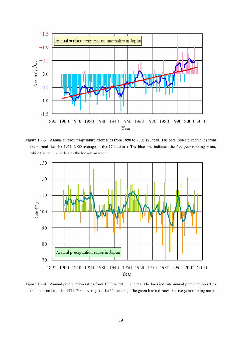
2.3 Surface temperature and precipitation in Japan

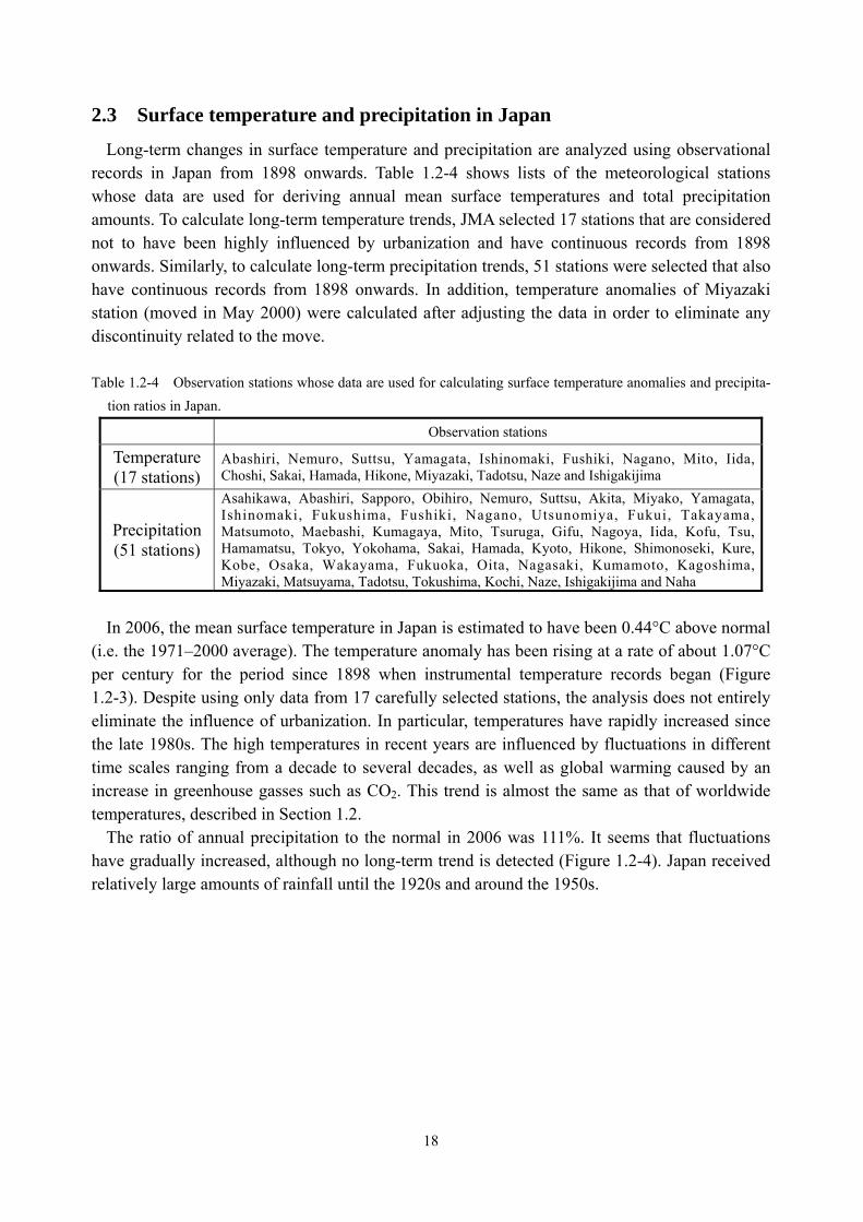
Long-term changes in surface temperature and precipitation are analyzed using observational records in Japan from 1898 onwards. Table 1.2-4 shows lists of the meteorological stations whose data are used for deriving annual mean surface temperatures and total precipitation amounts. To calculate long-term temperature trends, JMA selected 17 stations that are considered not to have been highly influenced by urbanization and have continuous records from 1898 onwards. Similarly, to calculate long-term precipitation trends, 51 stations were selected that also have continuous records from 1898 onwards. In addition, temperature anomalies of Miyazaki station (moved in May 2000) were calculated after adjusting the data in order to eliminate any discontinuity related to the move.

Table 1.2-4 Observation stations whose data are used for calculating surface temperature anomalies and precipita-

tion ratios in Japan.

Observation stations

Temperature (17 stations)

Abashiri, Nemuro, Suttsu, Yamagata, Ishinomaki, Fushiki, Nagano, Mito, Iida, Choshi, Sakai, Hamada, Hikone, Miyazaki, Tadotsu, Naze and Ishigakijima

Precipitation (51 stations)

Asahikawa, Abashiri, Sapporo, Obihiro, Nemuro, Suttsu, Akita, Miyako, Yamagata, Ishinomaki, Fukushima, Fushiki, Nagano, Utsunomiya, Fukui, Takayama, Matsumoto, Maebashi, Kumagaya, Mito, Tsuruga, Gifu, Nagoya, Iida, Kofu, Tsu, Hamamatsu, Tokyo, Yokohama, Sakai, Hamada, Kyoto, Hikone, Shimonoseki, Kure, Kobe, Osaka, Wakayama, Fukuoka, Oita, Nagasaki, Kumamoto, Kagoshima, Miyazaki, Matsuyama, Tadotsu, Tokushima, Kochi, Naze, Ishigakijima and Naha

In 2006, the mean surface temperature in Japan is estimated to have been 0.44°C above normal

(i.e. the 1971–2000 average). The temperature anomaly has been rising at a rate of about 1.07°C per century for the period since 1898 when instrumental temperature records began (Figure 1.2-3). Despite using only data from 17 carefully selected stations, the analysis does not entirely eliminate the influence of urbanization. In particular, temperatures have rapidly increased since the late 1980s. The high temperatures in recent years are influenced by fluctuations in different time scales ranging from a decade to several decades, as well as global warming caused by an increase in greenhouse gasses such as CO2. This trend is almost the same as that of worldwide temperatures, described in Section 1.2.

The ratio of annual precipitation to the normal in 2006 was 111%. It seems that fluctuations have gradually increased, although no long-term trend is detected (Figure 1.2-4). Japan received relatively large amounts of rainfall until the 1920s and around the 1950s.

19

Figure 1.2-3 Annual surface temperature anomalies from 1898 to 2006 in Japan. The bars indicate anomalies from the normal (i.e. the 1971–2000 average of the 17 stations). The blue line indicates the five-year running mean, while the red line indicates the long-term trend.

Figure 1.2-4 Annual precipitation ratios from 1898 to 2006 in Japan. The bars indicate annual precipitation ratios

to the normal (i.e. the 1971–2000 average of the 51 stations). The green line indicates the five-year running mean.

20

2.4 Long-term trend of extreme events in Japan

The trends of extreme climatic events in Japan are described in this section: extreme monthly mean temperatures and monthly precipitation amounts, and the number of days with extreme temperatures or precipitation amounts above certain thresholds (e.g. 30ºC, 100 mm). The observation stations used for this research are the same 17 for temperature and 51 for precipitation in Section 2.3 (see Table 1.2-4).

2.4.1 Long-term trend of extreme temperatures (1) Extreme monthly mean temperatures

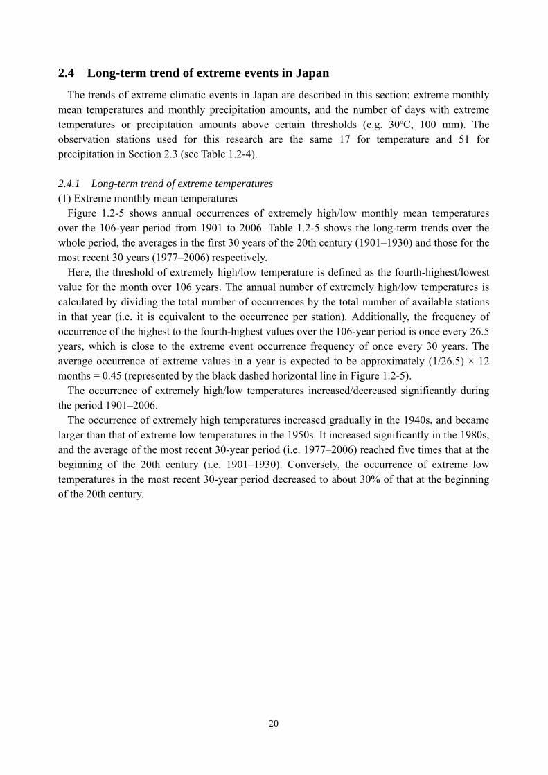
Figure 1.2-5 shows annual occurrences of extremely high/low monthly mean temperatures over the 106-year period from 1901 to 2006. Table 1.2-5 shows the long-term trends over the whole period, the averages in the first 30 years of the 20th century (1901–1930) and those for the most recent 30 years (1977–2006) respectively.

Here, the threshold of extremely high/low temperature is defined as the fourth-highest/lowest value for the month over 106 years. The annual number of extremely high/low temperatures is calculated by dividing the total number of occurrences by the total number of available stations in that year (i.e. it is equivalent to the occurrence per station). Additionally, the frequency of occurrence of the highest to the fourth-highest values over the 106-year period is once every 26.5 years, which is close to the extreme event occurrence frequency of once every 30 years. The average occurrence of extreme values in a year is expected to be approximately (1/26.5) × 12 months = 0.45 (represented by the black dashed horizontal line in Figure 1.2-5).

The occurrence of extremely high/low temperatures increased/decreased significantly during the period 1901–2006.

The occurrence of extremely high temperatures increased gradually in the 1940s, and became larger than that of extreme low temperatures in the 1950s. It increased significantly in the 1980s, and the average of the most recent 30-year period (i.e. 1977–2006) reached five times that at the beginning of the 20th century (i.e. 1901–1930). Conversely, the occurrence of extreme low temperatures in the most recent 30-year period decreased to about 30% of that at the beginning of the 20th century.

21

Figure 1.2-5 Annual number of occurrences of extremely high/low monthly mean temperatures

The annual number of occurrences of the highest/lowest first-to-fourth values for each month during the period 1901–2006 are indicated. The thin blue/red lines indicate the annual occurrence of extremely high/low monthly mean temperatures divided by the total number of monthly observation data sets available in the year (i.e. the average occurrence per station). The thick blue/red lines indicate the 11-year running mean value. The thick dashed black line indicates the expected frequency of the highest/lowest first-to-fourth values for each month over the 106-year period.

Table 1.2-5 Long-term trends of extremely high/low monthly temperatures

The long-term trend refers to the linear trend and the occurrence per station per ten-year period. The asterisk (*) means that the trend is significant at a 95% confidence level. The average occurrence per station during the first 30 years of the 20th century (i.e. 1901–1930) and the most recent 30-year period (i.e. 1977–2006) are also indicated respectively.

Extremely high monthly temperatures

Average of 1901–1930 0.21 Trend for 1901–2006: +0.11 /10 years (*) Average of 1977–2006 1.06

Extremely low monthly temperatures

Average of 1901–1930 0.78 Trend for 1901–2006: -0.08 /10 years (*) Average of 1977–2006 0.23

(2) Annual number of days with maximum temperatures ≥30ºC and ≥35ºC

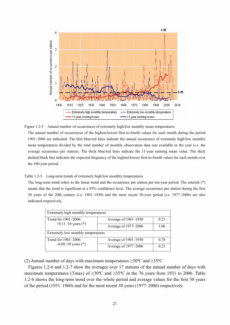
Figures 1.2-6 and 1.2-7 show the averages over 17 stations of the annual number of days with maximum temperatures (Tmax) of ≥30ºC and ≥35ºC in the 76 years from 1931 to 2006. Table 1.2-6 shows the long-term trend over the whole period and average values for the first 30 years of the period (1931–1960) and for the most recent 30 years (1977–2006) respectively.

22

Here, where there are months in which the number of days with missing observation data is more than 20% of the total, the annual data for the year at that station are not used in the calculation above. The same process is followed in part (3) of this section and in part (2) of Section 2.4.2.

The annual number of days with Tmax≥30ºC shows no significant trend in the period 1931–2006, and there is little difference between the averages of the first 30 years and the most recent 30 years. However, an increasing trend has been seen since the 1980s, and the most recent 11-year average is the highest since 1931.

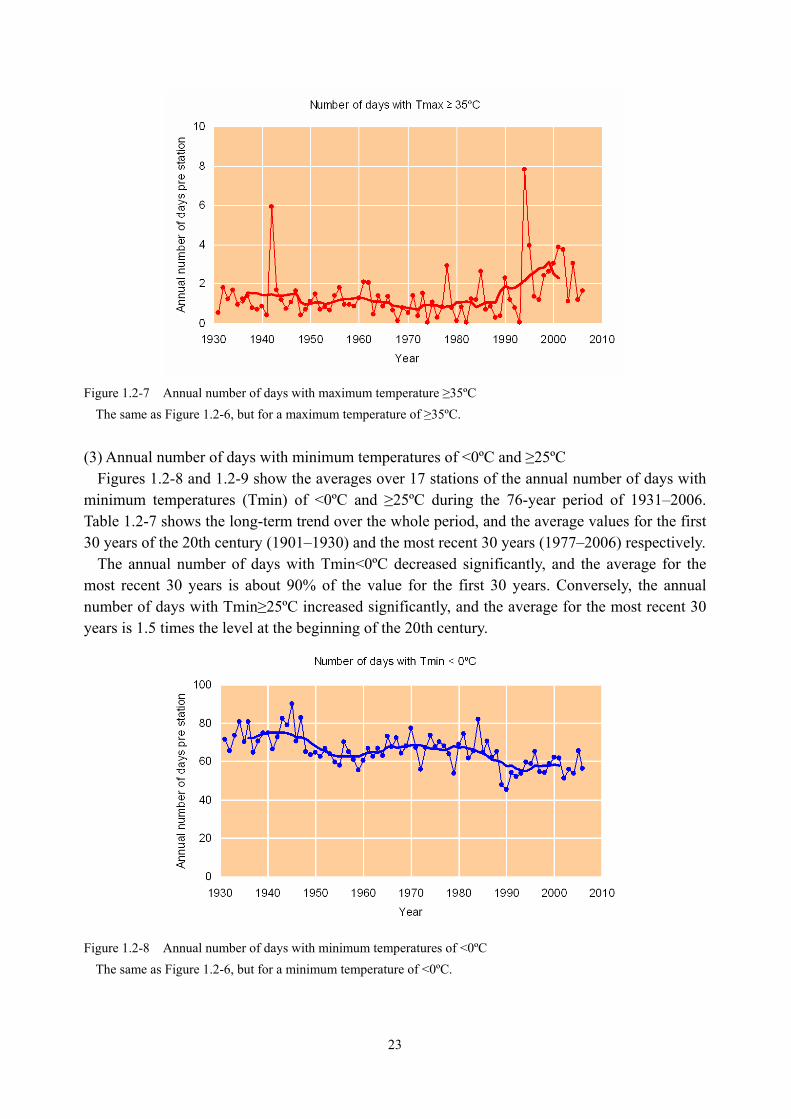
The annual number of days with Tmax≥35ºC increased significantly in the period 1931–2006, and the average of the most recent 30 years reached 1.5 times that of 1931–1960. No large variability was seen until the 1970s, but the level increased in the 1980s and has often been more than two days per station since the middle of the 1990s.

Table 1.2-6 Long-term trends in the annual number of days with maximum temperatures of ≥30ºC and ≥35ºC

The table is the same as that in 1-2.5, except the trend during the period 1931–2006 is indicated as the change every 10 years (unit: day/station). The average occurrences per station in the first 30 years (1931–1960) and the most recent 30 years (1977–2006) are also indicated respectively.

Annual number of days with Tmax≥30ºC

Average of 1931–1960 38.4 days Trend in 1931–2006: +0.19 days/10 years Average of 1977–2006 38.8 days

Annual number of days with Tmax≥35ºC

Average of 1931–1960 1.2 days Trend in 1931–2006: +0.14 days/10 years (*) Average of 1977–2006 1.8 days

Figure 1.2-6 Annual number of days with maximum temperature ≥30ºC

Annual number of days per station. The thin line indicates the value for each year, and the thick line indicates the 11-year running mean value.

23

Figure 1.2-7 Annual number of days with maximum temperature ≥35ºC

The same as Figure 1.2-6, but for a maximum temperature of ≥35ºC.

(3) Annual number of days with minimum temperatures of <0ºC and ≥25ºC

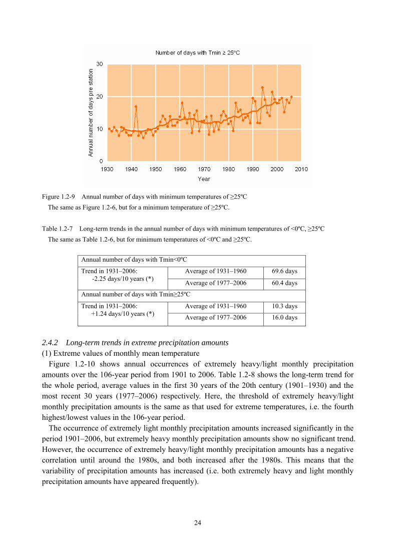
Figures 1.2-8 and 1.2-9 show the averages over 17 stations of the annual number of days with minimum temperatures (Tmin) of <0ºC and ≥25ºC during the 76-year period of 1931–2006. Table 1.2-7 shows the long-term trend over the whole period, and the average values for the first 30 years of the 20th century (1901–1930) and the most recent 30 years (1977–2006) respectively.

The annual number of days with Tmin<0ºC decreased significantly, and the average for the most recent 30 years is about 90% of the value for the first 30 years. Conversely, the annual number of days with Tmin≥25ºC increased significantly, and the average for the most recent 30 years is 1.5 times the level at the beginning of the 20th century.

Figure 1.2-8 Annual number of days with minimum temperatures of <0ºC

The same as Figure 1.2-6, but for a minimum temperature of <0ºC.

24

Figure 1.2-9 Annual number of days with minimum temperatures of ≥25ºC

The same as Figure 1.2-6, but for a minimum temperature of ≥25ºC. Table 1.2-7 Long-term trends in the annual number of days with minimum temperatures of <0ºC, ≥25ºC

The same as Table 1.2-6, but for minimum temperatures of <0ºC and ≥25ºC.

Annual number of days with Tmin<0ºC

Average of 1931–1960 69.6 days Trend in 1931–2006: -2.25 days/10 years (*) Average of 1977–2006 60.4 days

Annual number of days with Tmin≥25ºC

Average of 1931–1960 10.3 days Trend in 1931–2006: +1.24 days/10 years (*) Average of 1977–2006 16.0 days

2.4.2 Long-term trends in extreme precipitation amounts (1) Extreme values of monthly mean temperature

Figure 1.2-10 shows annual occurrences of extremely heavy/light monthly precipitation amounts over the 106-year period from 1901 to 2006. Table 1.2-8 shows the long-term trend for the whole period, average values in the first 30 years of the 20th century (1901–1930) and the most recent 30 years (1977–2006) respectively. Here, the threshold of extremely heavy/light monthly precipitation amounts is the same as that used for extreme temperatures, i.e. the fourth highest/lowest values in the 106-year period.

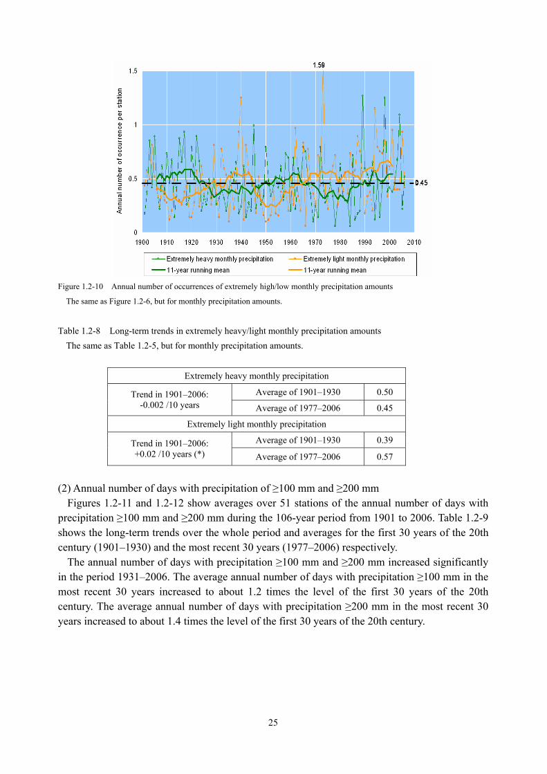
The occurrence of extremely light monthly precipitation amounts increased significantly in the period 1901–2006, but extremely heavy monthly precipitation amounts show no significant trend. However, the occurrence of extremely heavy/light monthly precipitation amounts has a negative correlation until around the 1980s, and both increased after the 1980s. This means that the variability of precipitation amounts has increased (i.e. both extremely heavy and light monthly precipitation amounts have appeared frequently).

25

Figure 1.2-10 Annual number of occurrences of extremely high/low monthly precipitation amounts

The same as Figure 1.2-6, but for monthly precipitation amounts.

Table 1.2-8 Long-term trends in extremely heavy/light monthly precipitation amounts The same as Table 1.2-5, but for monthly precipitation amounts.

Extremely heavy monthly precipitation

Average of 1901–1930 0.50 Trend in 1901–2006: -0.002 /10 years Average of 1977–2006 0.45

Extremely light monthly precipitation

Average of 1901–1930 0.39 Trend in 1901–2006: +0.02 /10 years (*) Average of 1977–2006 0.57

(2) Annual number of days with precipitation of ≥100 mm and ≥200 mm

Figures 1.2-11 and 1.2-12 show averages over 51 stations of the annual number of days with precipitation ≥100 mm and ≥200 mm during the 106-year period from 1901 to 2006. Table 1.2-9 shows the long-term trends over the whole period and averages for the first 30 years of the 20th century (1901–1930) and the most recent 30 years (1977–2006) respectively.

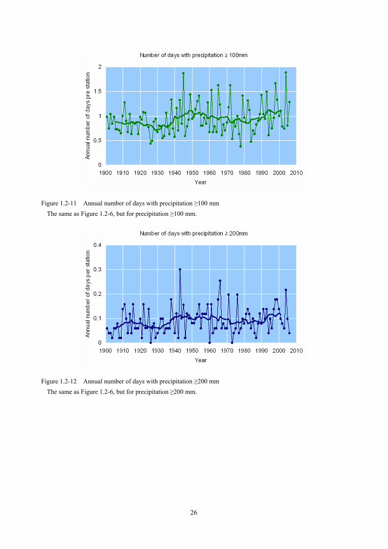
The annual number of days with precipitation ≥100 mm and ≥200 mm increased significantly in the period 1931–2006. The average annual number of days with precipitation ≥100 mm in the most recent 30 years increased to about 1.2 times the level of the first 30 years of the 20th century. The average annual number of days with precipitation ≥200 mm in the most recent 30 years increased to about 1.4 times the level of the first 30 years of the 20th century.

26

Figure 1.2-11 Annual number of days with precipitation ≥100 mm The same as Figure 1.2-6, but for precipitation ≥100 mm.

Figure 1.2-12 Annual number of days with precipitation ≥200 mm The same as Figure 1.2-6, but for precipitation ≥200 mm.

27

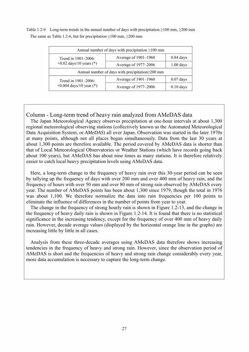
Table 1.2-9 Long-term trends in the annual number of days with precipitation ≥100 mm, ≥200 mm The same as Table 1.2-6, but for precipitation ≥100 mm, ≥200 mm.

Annual number of days with precipitation ≥100 mm

Average of 1901–1960 0.84 days Trend in 1901–2006: +0.02 days/10 years (*) Average of 1977–2006 1.00 days

Annual number of days with precipitation≥200 mm

Average of 1901–1960 0.07 days Trend in 1901–2006: +0.004 days/10 year (*) Average of 1977–2006 0.10 days

Column - Long-term trend of heavy rain analyzed from AMeDAS data

The Japan Meteorological Agency observes precipitation at one-hour intervals at about 1,300 regional meteorological observing stations (collectively known as the Automated Meteorological Data Acquisition System, or AMeDAS) all over Japan. Observation was started in the later 1970s at many points, although not all places began simultaneously. Data from the last 30 years at about 1,300 points are therefore available. The period covered by AMeDAS data is shorter than that of Local Meteorological Observatories or Weather Stations (which have records going back about 100 years), but AMeDAS has about nine times as many stations. It is therefore relatively easier to catch local heavy precipitation levels using AMeDAS data.

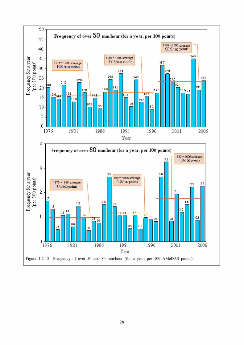
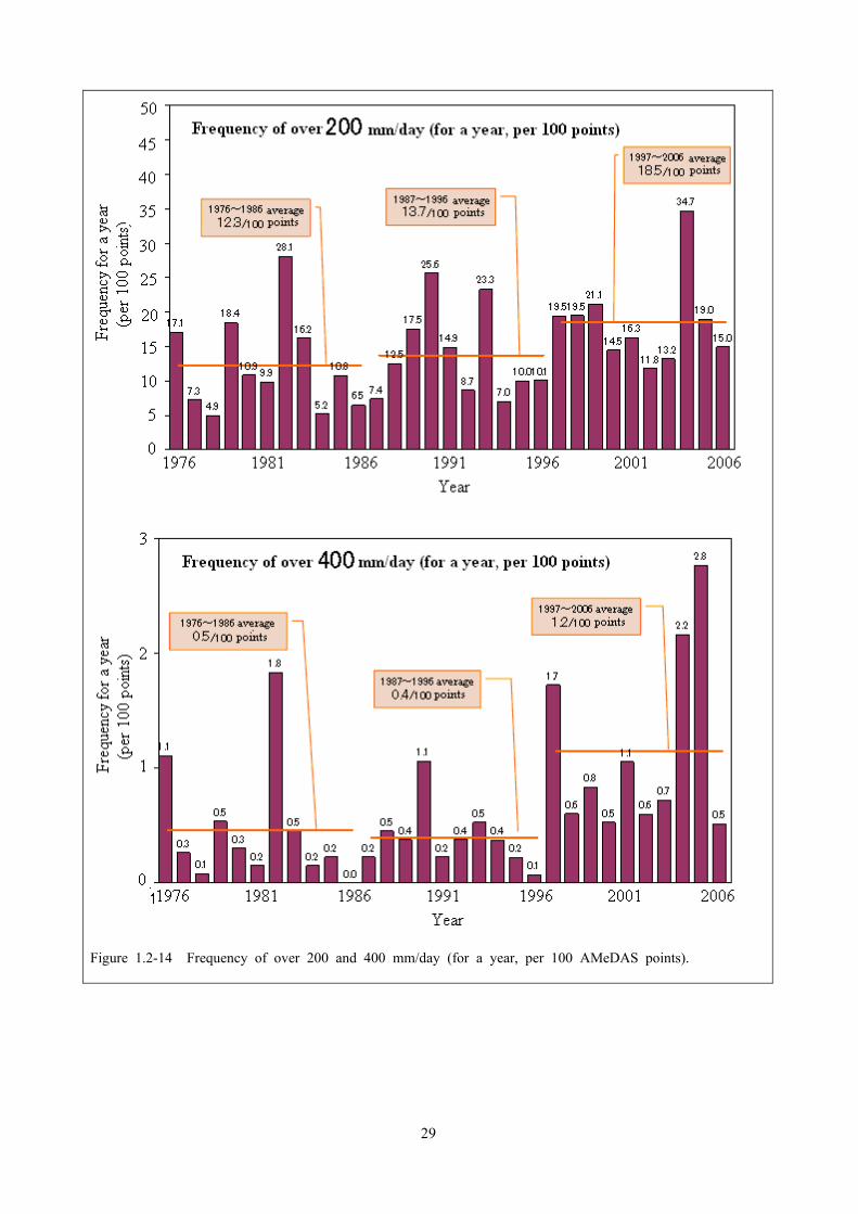
Here, a long-term change in the frequency of heavy rain over this 30-year period can be seen

by tallying up the frequency of days with over 200 mm and over 400 mm of heavy rain, and the frequency of hours with over 50 mm and over 80 mm of strong rain observed by AMeDAS every year. The number of AMeDAS points has been about 1,300 since 1979, though the total in 1976 was about 1,100. We therefore normalize the data into rain frequencies per 100 points to eliminate the influence of differences in the number of points from year to year.

The change in the frequency of strong hourly rain is shown in Figure 1.2-13, and the change in the frequency of heavy daily rain is shown in Figure 1.2-14. It is found that there is no statistical significance in the increasing tendency, except for the frequency of over 400 mm of heavy daily rain. However, decade average values (displayed by the horizontal orange line in the graphs) are increasing little by little in all cases.

Analysis from these three-decade averages using AMeDAS data therefore shows increasing

tendencies in the frequency of heavy and strong rain. However, since the observation period of AMeDAS is short and the frequencies of heavy and strong rain change considerably every year, more data accumulation is necessary to capture the long-term change.

28

Figure 1.2-13 Frequency of over 50 and 80 mm/hour (for a year, per 100 AMeDAS points).

29

Figure 1.2-14 Frequency of over 200 and 400 mm/day (for a year, per 100 AMeDAS points).

30

2.5 Tropical cyclones

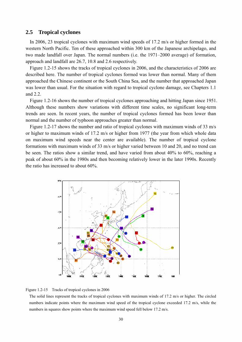
In 2006, 23 tropical cyclones with maximum wind speeds of 17.2 m/s or higher formed in the western North Pacific. Ten of these approached within 300 km of the Japanese archipelago, and two made landfall over Japan. The normal numbers (i.e. the 1971–2000 average) of formation, approach and landfall are 26.7, 10.8 and 2.6 respectively.

Figure 1.2-15 shows the tracks of tropical cyclones in 2006, and the characteristics of 2006 are described here. The number of tropical cyclones formed was lower than normal. Many of them approached the Chinese continent or the South China Sea, and the number that approached Japan was lower than usual. For the situation with regard to tropical cyclone damage, see Chapters 1.1 and 2.2.

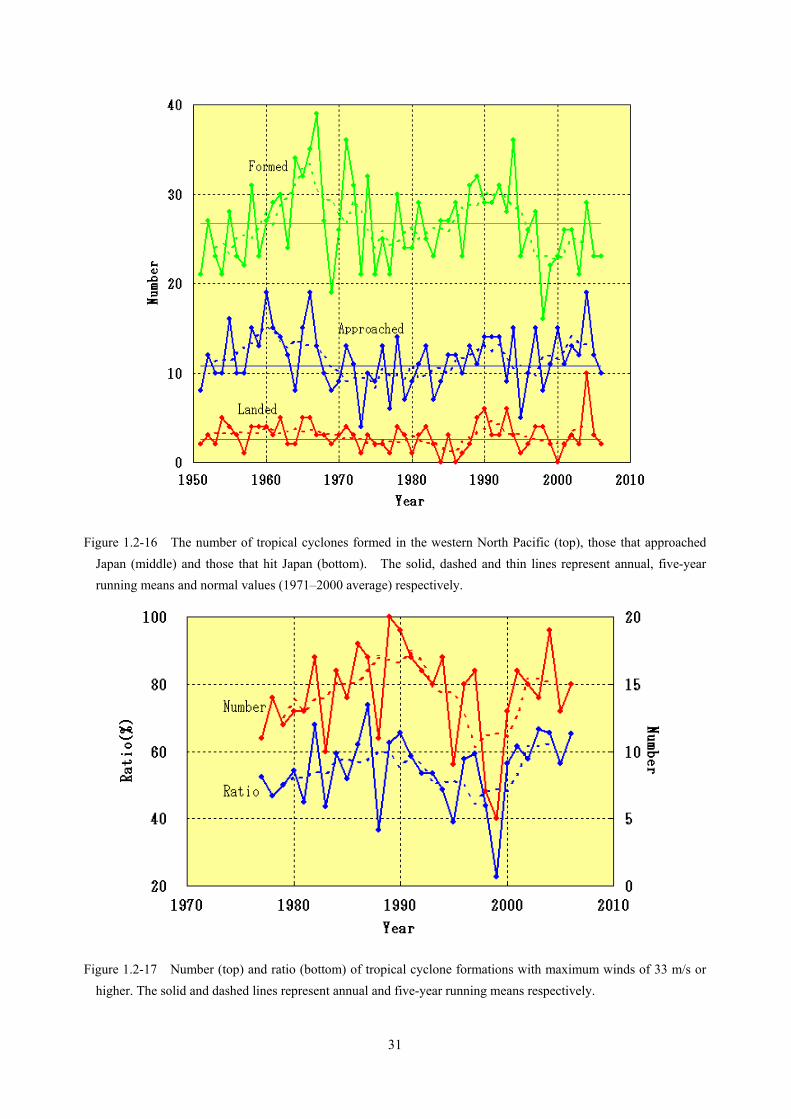
Figure 1.2-16 shows the number of tropical cyclones approaching and hitting Japan since 1951. Although these numbers show variations with different time scales, no significant long-term trends are seen. In recent years, the number of tropical cyclones formed has been lower than normal and the number of typhoon approaches greater than normal.

Figure 1.2-17 shows the number and ratio of tropical cyclones with maximum winds of 33 m/s or higher to maximum winds of 17.2 m/s or higher from 1977 (the year from which whole data on maximum wind speeds near the center are available). The number of tropical cyclone formations with maximum winds of 33 m/s or higher varied between 10 and 20, and no trend can be seen. The ratios show a similar trend, and have varied from about 40% to 60%, reaching a peak of about 60% in the 1980s and then becoming relatively lower in the later 1990s. Recently the ratio has increased to about 60%.

Figure 1.2-15 Tracks of tropical cyclones in 2006

The solid lines represent the tracks of tropical cyclones with maximum winds of 17.2 m/s or higher. The circled numbers indicate points where the maximum wind speed of the tropical cyclone exceeded 17.2 m/s, while the numbers in squares show points where the maximum wind speed fell below 17.2 m/s.

31

Figure 1.2-16 The number of tropical cyclones formed in the western North Pacific (top), those that approached Japan (middle) and those that hit Japan (bottom). The solid, dashed and thin lines represent annual, five-year running means and normal values (1971–2000 average) respectively.

Figure 1.2-17 Number (top) and ratio (bottom) of tropical cyclone formations with maximum winds of 33 m/s or

higher. The solid and dashed lines represent annual and five-year running means respectively.

32

2.6 Urban heat island effects in metropolitan areas of Japan

In order to contribute toward formulating policies for the mitigation of urban heat island (UHI) effects, the Japan Meteorological Agency (JMA) has conducted research into how UHI actually influences urban climates and what kind of weather conditions are likely to aggravate its impact. In 2006, JMA carried out a case study on the UHI effects occurring in the Kinki and Kanto regions on typical summer days.

2.6.1 Temperature trend in Japan’s metropolitan areas

In July 2006, monthly mean temperatures were near normal across the Kinki region, in spite of sunshine durations that were below normal at many observation stations in Kinki primarily due to the Baiu front’s activity. In August, dominant high pressure systems brought above-normal sunshine durations to the region, leading to monthly mean temperatures that were more than one degree above normal at most stations. In Kyoto, Osaka and Nara in particular, mean maximum temperatures two degrees above normal were recorded. Meanwhile, monthly mean temperatures in the Kanto region for July 2006 were below or near normal at most stations, chiefly due to below-normal sunshine durations associated with the Baiu front’s activity. In August, however, temperatures were above normal in terms of the monthly mean and the mean daily maximum, as well as the mean daily minimum. Sunshine durations were below or near normal at most stations, which indicates that synoptic weather conditions were rarely favorable to the development of significant UHI effects.

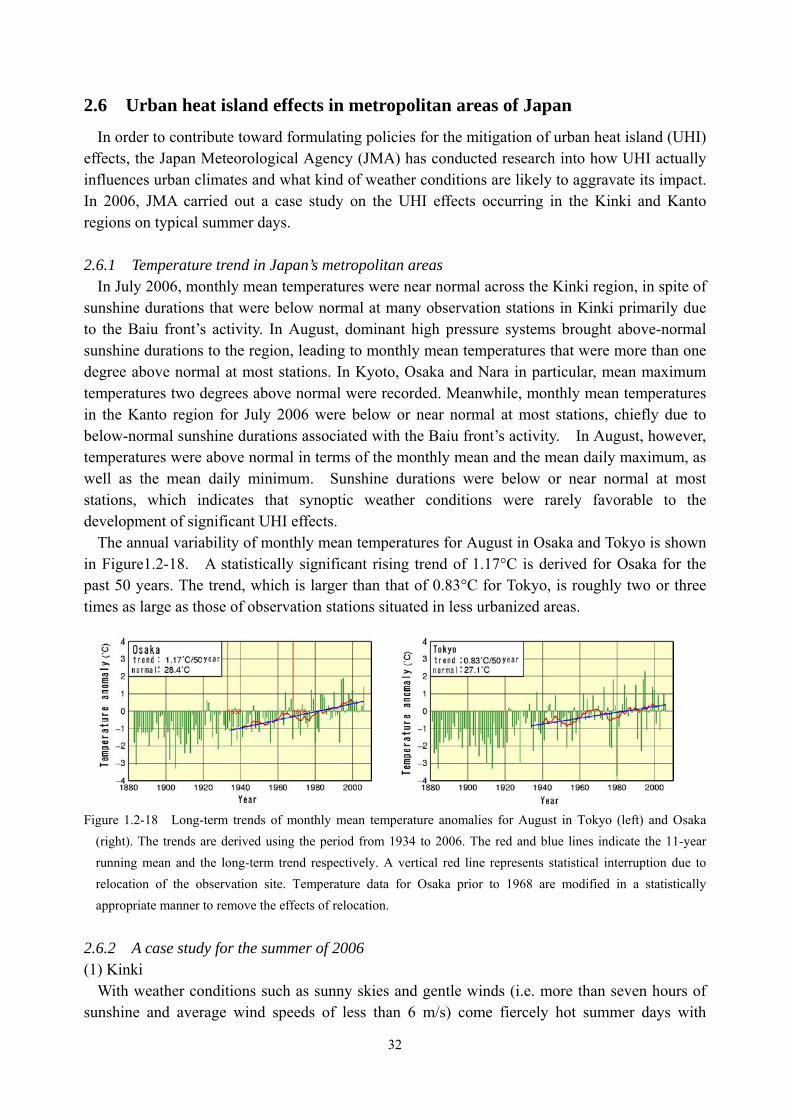
The annual variability of monthly mean temperatures for August in Osaka and Tokyo is shown in Figure1.2-18. A statistically significant rising trend of 1.17°C is derived for Osaka for the past 50 years. The trend, which is larger than that of 0.83°C for Tokyo, is roughly two or three times as large as those of observation stations situated in less urbanized areas.

Figure 1.2-18 Long-term trends of monthly mean temperature anomalies for August in Tokyo (left) and Osaka

(right). The trends are derived using the period from 1934 to 2006. The red and blue lines indicate the 11-year running mean and the long-term trend respectively. A vertical red line represents statistical interruption due to relocation of the observation site. Temperature data for Osaka prior to 1968 are modified in a statistically appropriate manner to remove the effects of relocation.

2.6.2 A case study for the summer of 2006 (1) Kinki

With weather conditions such as sunny skies and gentle winds (i.e. more than seven hours of sunshine and average wind speeds of less than 6 m/s) come fiercely hot summer days with

33

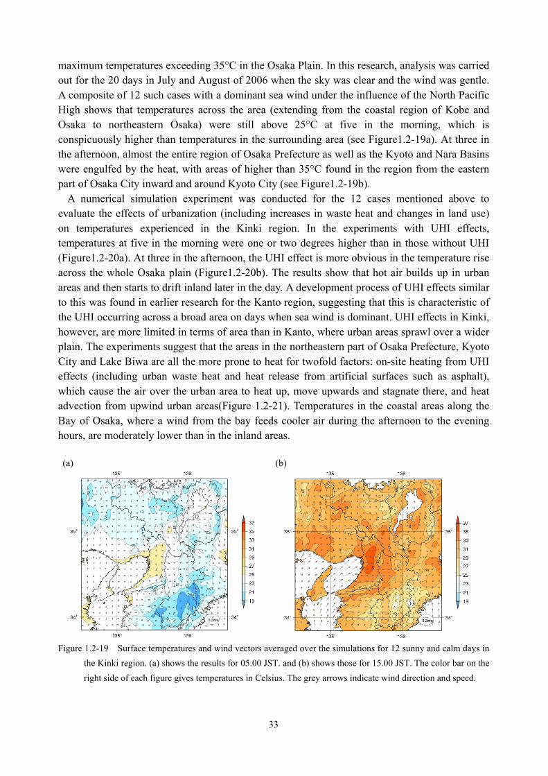
maximum temperatures exceeding 35°C in the Osaka Plain. In this research, analysis was carried out for the 20 days in July and August of 2006 when the sky was clear and the wind was gentle. A composite of 12 such cases with a dominant sea wind under the influence of the North Pacific High shows that temperatures across the area (extending from the coastal region of Kobe and Osaka to northeastern Osaka) were still above 25°C at five in the morning, which is conspicuously higher than temperatures in the surrounding area (see Figure1.2-19a). At three in the afternoon, almost the entire region of Osaka Prefecture as well as the Kyoto and Nara Basins were engulfed by the heat, with areas of higher than 35°C found in the region from the eastern part of Osaka City inward and around Kyoto City (see Figure1.2-19b).

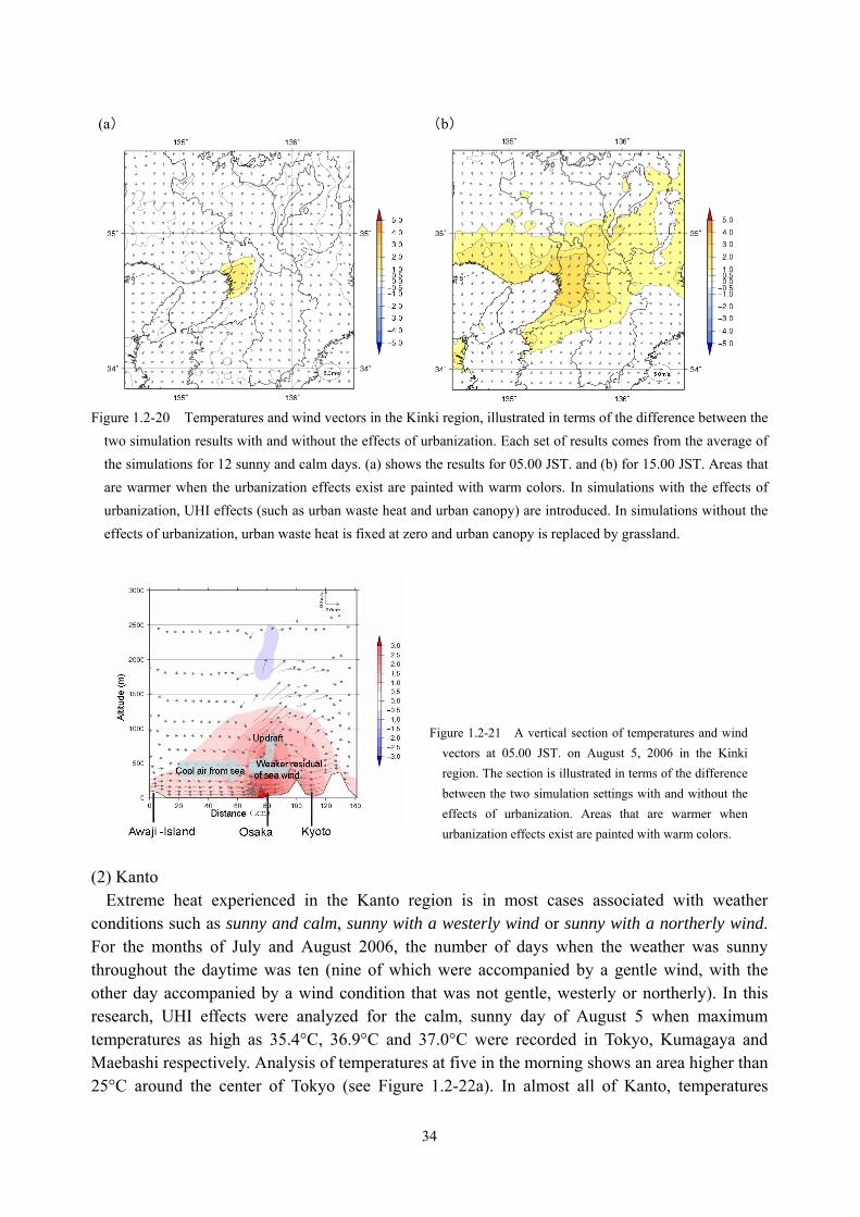
A numerical simulation experiment was conducted for the 12 cases mentioned above to evaluate the effects of urbanization (including increases in waste heat and changes in land use) on temperatures experienced in the Kinki region. In the experiments with UHI effects, temperatures at five in the morning were one or two degrees higher than in those without UHI (Figure1.2-20a). At three in the afternoon, the UHI effect is more obvious in the temperature rise across the whole Osaka plain (Figure1.2-20b). The results show that hot air builds up in urban areas and then starts to drift inland later in the day. A development process of UHI effects similar to this was found in earlier research for the Kanto region, suggesting that this is characteristic of the UHI occurring across a broad area on days when sea wind is dominant. UHI effects in Kinki, however, are more limited in terms of area than in Kanto, where urban areas sprawl over a wider plain. The experiments suggest that the areas in the northeastern part of Osaka Prefecture, Kyoto City and Lake Biwa are all the more prone to heat for twofold factors: on-site heating from UHI effects (including urban waste heat and heat release from artificial surfaces such as asphalt), which cause the air over the urban area to heat up, move upwards and stagnate there, and heat advection from upwind urban areas(Figure 1.2-21). Temperatures in the coastal areas along the Bay of Osaka, where a wind from the bay feeds cooler air during the afternoon to the evening hours, are moderately lower than in the inland areas.

(a) (b)

Figure 1.2-19 Surface temperatures and wind vectors averaged over the simulations for 12 sunny and calm days in

the Kinki region. (a) shows the results for 05.00 JST. and (b) shows those for 15.00 JST. The color bar on the right side of each figure gives temperatures in Celsius. The grey arrows indicate wind direction and speed.

34

(a） （b）

Figure 1.2-20 Temperatures and wind vectors in the Kinki region, illustrated in terms of the difference between the

two simulation results with and without the effects of urbanization. Each set of results comes from the average of the simulations for 12 sunny and calm days. (a) shows the results for 05.00 JST. and (b) for 15.00 JST. Areas that are warmer when the urbanization effects exist are painted with warm colors. In simulations with the effects of urbanization, UHI effects (such as urban waste heat and urban canopy) are introduced. In simulations without the effects of urbanization, urban waste heat is fixed at zero and urban canopy is replaced by grassland.

Figure 1.2-21 A vertical section of temperatures and wind vectors at 05.00 JST. on August 5, 2006 in the Kinki region. The section is illustrated in terms of the difference between the two simulation settings with and without the effects of urbanization. Areas that are warmer when urbanization effects exist are painted with warm colors.

(2) Kanto

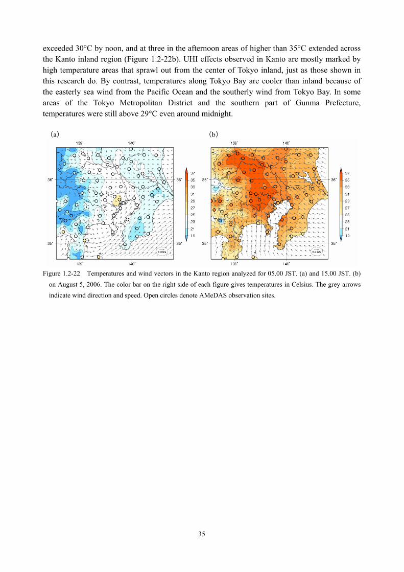
Extreme heat experienced in the Kanto region is in most cases associated with weather conditions such as sunny and calm, sunny with a westerly wind or sunny with a northerly wind. For the months of July and August 2006, the number of days when the weather was sunny throughout the daytime was ten (nine of which were accompanied by a gentle wind, with the other day accompanied by a wind condition that was not gentle, westerly or northerly). In this research, UHI effects were analyzed for the calm, sunny day of August 5 when maximum temperatures as high as 35.4°C, 36.9°C and 37.0°C were recorded in Tokyo, Kumagaya and Maebashi respectively. Analysis of temperatures at five in the morning shows an area higher than 25°C around the center of Tokyo (see Figure 1.2-22a). In almost all of Kanto, temperatures

35

exceeded 30°C by noon, and at three in the afternoon areas of higher than 35°C extended across the Kanto inland region (Figure 1.2-22b). UHI effects observed in Kanto are mostly marked by high temperature areas that sprawl out from the center of Tokyo inland, just as those shown in this research do. By contrast, temperatures along Tokyo Bay are cooler than inland because of the easterly sea wind from the Pacific Ocean and the southerly wind from Tokyo Bay. In some areas of the Tokyo Metropolitan District and the southern part of Gunma Prefecture, temperatures were still above 29°C even around midnight. （a） （b）

Figure 1.2-22 Temperatures and wind vectors in the Kanto region analyzed for 05.00 JST. (a) and 15.00 JST. (b) on August 5, 2006. The color bar on the right side of each figure gives temperatures in Celsius. The grey arrows indicate wind direction and speed. Open circles denote AMeDAS observation sites.

36

Part II Oceans Oceans, which cover about 70 percent of the earth's surface, are a major component of the

climate system and have a significant effect on the motion of the atmosphere. In order to monitor oceans, the Japan Meteorological Agency conducts various kinds of oceanographic observation such as research vessel surveys and deployment of ocean data buoys and profiling floats. Based on these observational data as well as satellite observations and reports from voluntary merchant ships and fishing boats, oceanographic conditions such as water temperature distribution and ocean currents are analyzed using modern technology including numerical models. In addition to the monitoring of these physical parameters, JMA conducts regular surveys to monitor marine pollution. The results of ocean monitoring in 2006 are summarized in this chapter. Details of the monitoring results and recent information are available on the Marine Diagnosis Report web site (in Japanese) at http://www.data.kishou.go.jp/kaiyou/shindan/.

1 Global Oceans

1.1 Global sea surface temperature

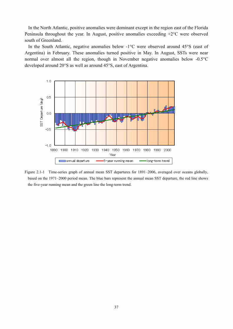
Figure 2.1-1 shows the long-term rising trend (0.50°C per century) in the global average sea surface temperature (SST), represented in the form of departure from the 1971–2000 mean. The 2006 SST departure was +0.21°C, which is ranked as the second highest since 1900, next only to 1998 and parallel with 2002, 2003 and 2005.

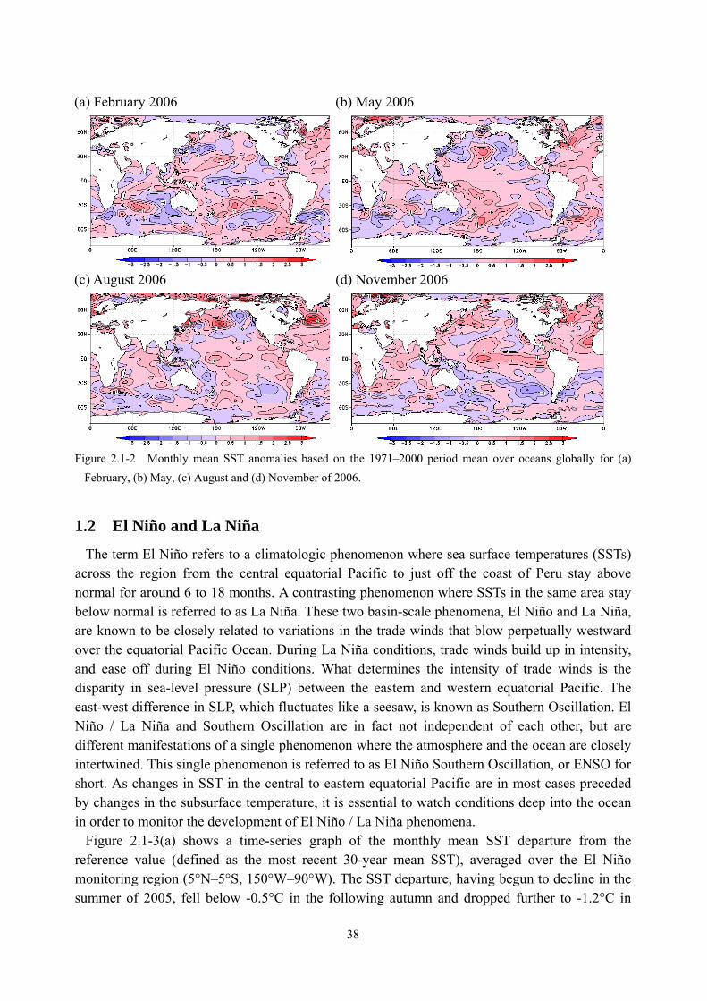
Figure 2.1-2 shows the global SST anomalies based on the 1971–2000 mean for February, May, August and November of 2006. In the mid to high latitude of the North Pacific, negative anomalies were observed in the western region from February through May, although these had disappeared by November. In February, positive anomalies exceeding +1°C developed at around 30°N in the central region. The positive anomaly area began to move northward with increased intensity, resulting in positive anomalies exceeding +2°C at around 40°N in August. In the eastern region, negative anomalies below -1°C were observed around 30°N in May and south of Alaska in August. Both of these negative anomalies had mostly vanished by November.

In the equatorial Pacific Ocean, negative anomalies exceeding -1°C were observed in February in the region from the date line to 120°W. These negative anomalies had disappeared by May, and SSTs then returned to near normal all over the equatorial Pacific. In August, however, positive anomalies exceeding +1°C began to develop in the vicinity of the date line and off the coast of South America. By November, the whole region east of the date line had been covered with positive anomalies.

In the mid to high latitude of the South Pacific Ocean, positive anomalies were observed stretching east and west around 30°S in February. The eastern part of these positive anomalies had disappeared by May. Negative anomalies were observed around 45°S in the eastern South Pacific from February, and eventually developed into anomalies below -1°C in November.

In the mid to high latitude of the Indian Ocean, negative anomalies below -1°C and positive anomalies exceeding +1°C were observed west of Australia and southeast of Madagascar respectively in February. Both of these anomalies had shrunk by May. In the equatorial Indian Ocean, a pattern of positive in the west and negative in the east had been sustained since August.

37

In the North Atlantic, positive anomalies were dominant except in the region east of the Florida Peninsula throughout the year. In August, positive anomalies exceeding +2°C were observed south of Greenland.

In the South Atlantic, negative anomalies below -1°C were observed around 45°S (east of Argentina) in February. These anomalies turned positive in May. In August, SSTs were near normal over almost all the region, though in November negative anomalies below -0.5°C developed around 20°S as well as around 45°S, east of Argentina.

Figure 2.1-1 Time-series graph of annual mean SST departures for 1891–2006, averaged over oceans globally,

based on the 1971–2000 period mean. The blue bars represent the annual mean SST departure, the red line shows the five-year running mean and the green line the long-term trend.

38

(a) February 2006 (b) May 2006

(c) August 2006 (d) November 2006

Figure 2.1-2 Monthly mean SST anomalies based on the 1971–2000 period mean over oceans globally for (a) February, (b) May, (c) August and (d) November of 2006.

1.2 El Niño and La Niña

The term El Niño refers to a climatologic phenomenon where sea surface temperatures (SSTs) across the region from the central equatorial Pacific to just off the coast of Peru stay above normal for around 6 to 18 months. A contrasting phenomenon where SSTs in the same area stay below normal is referred to as La Niña. These two basin-scale phenomena, El Niño and La Niña, are known to be closely related to variations in the trade winds that blow perpetually westward over the equatorial Pacific Ocean. During La Niña conditions, trade winds build up in intensity, and ease off during El Niño conditions. What determines the intensity of trade winds is the disparity in sea-level pressure (SLP) between the eastern and western equatorial Pacific. The east-west difference in SLP, which fluctuates like a seesaw, is known as Southern Oscillation. El Niño / La Niña and Southern Oscillation are in fact not independent of each other, but are different manifestations of a single phenomenon where the atmosphere and the ocean are closely intertwined. This single phenomenon is referred to as El Niño Southern Oscillation, or ENSO for short. As changes in SST in the central to eastern equatorial Pacific are in most cases preceded by changes in the subsurface temperature, it is essential to watch conditions deep into the ocean in order to monitor the development of El Niño / La Niña phenomena.

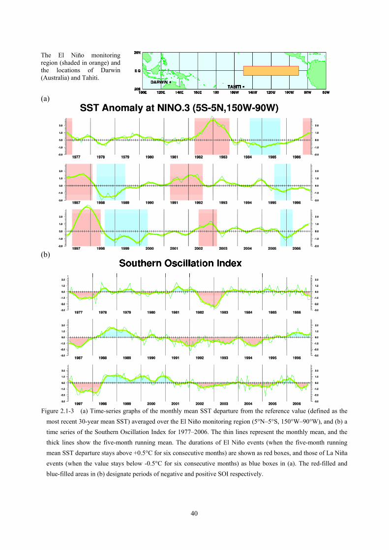
Figure 2.1-3(a) shows a time-series graph of the monthly mean SST departure from the reference value (defined as the most recent 30-year mean SST), averaged over the El Niño monitoring region (5°N–5°S, 150°W–90°W). The SST departure, having begun to decline in the summer of 2005, fell below -0.5°C in the following autumn and dropped further to -1.2°C in

39

December. The five-month running mean SST departure remained below -0.5°C all through the six-month period from the autumn of 2005 to the spring of 2006, thus fulfilling JMA’s criterion for a La Niña episode. From the spring of 2006 onwards, the SST departure was seen to rise, and turned positive in the following summer. In September, the five-month running mean departure reached +0.6°C. As of the end of 2006, the SST departure was still positive.

Figure 2.1-3(b) shows time-series graphs of the Southern Oscillation Index (SOI), which is defined as the difference between SLP anomalies observed at Tahiti in the Southern Pacific Ocean and at Darwin, Australia. Generally, SOI swings to the negative side during El Niño and to the positive side during La Niña. From the autumn of 2005 through the spring of 2006, the five-month running mean SOI continued to be positive (reflecting the ongoing La Niña episode), while the monthly mean SOI was seen fluctuating roughly on a two-month cycle. From the summer of 2006 onward, the monthly mean SOI turned negative in response to rising SST in the eastern Pacific. The negative SOI lasted until the end of 2006.

Figures 2.1-2 (a), (b), (c) and (d) show the monthly mean SST anomalies for February, May, August and November of 2006 respectively. In February, negative SST anomalies were observed extending from the vicinity of the date line to 120°W in the equatorial Pacific, although by May they had vanished and SSTs returned to near normal all over the region. From August, positive SST anomalies exceeding +1°C began to develop around the date line and off the coast of Peru. In November, positive SST anomalies were seen extending over the equatorial Pacific east of the date line.

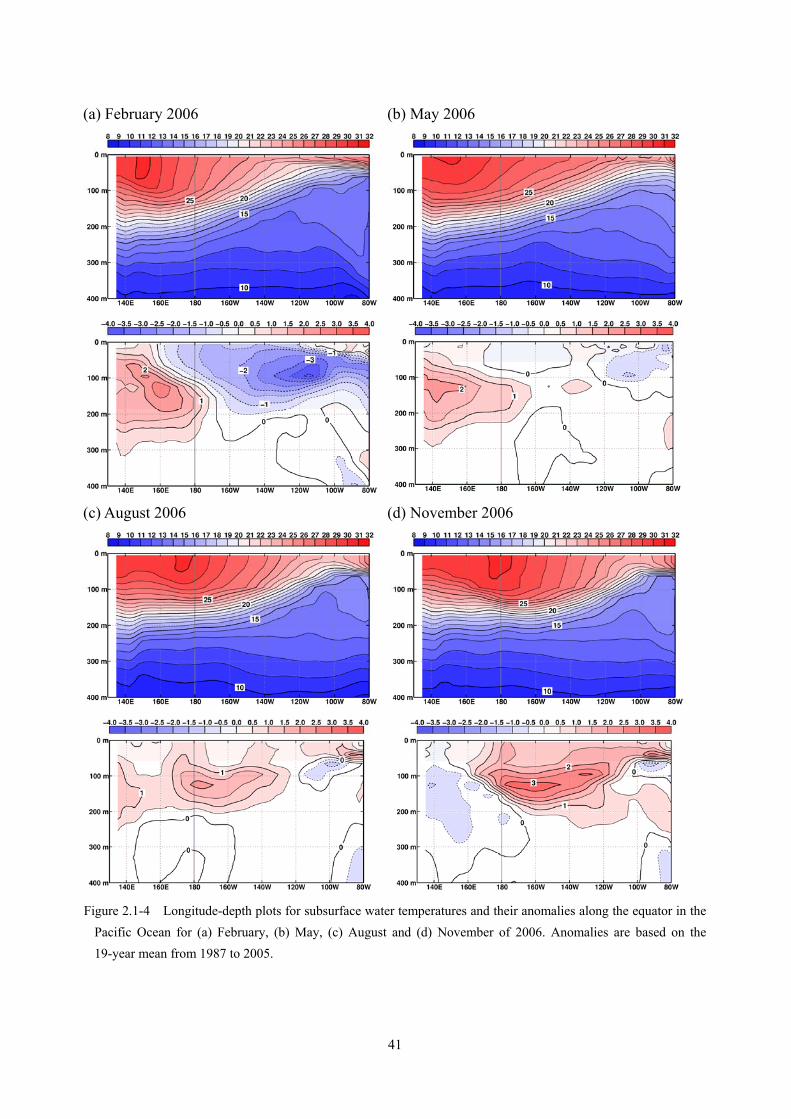
Figures 2.1-4 (a), (b), (c) and (d) show subsurface water temperatures and their anomalies down to a depth of 400 m along the equator in the Pacific Ocean for February, May, August and November of 2006. Under normal conditions, the thermocline, which is marked by a thin layer where the temperature drops abruptly with depth (roughly equivalent to the depth of the 20°C isothermal line), has an uphill gradient towards the east. In February 2006, the west-east gradient of the thermocline was enhanced, reflecting the positive temperature anomalies in the west and the negative ones in the east that were observed around the depth of the thermocline. During the subsequent months, positive anomalies in the west propagated eastward successively, which eventually caused the negative anomalies in the east to disappear. Positive temperature anomalies appeared off the coast of Peru in August, and extended all over the equatorial Pacific east of the date line.

40

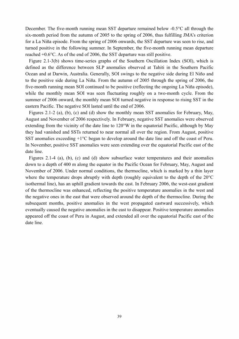
The El Niño monitoring region (shaded in orange) and the locations of Darwin (Australia) and Tahiti.

(a)

(b)

Figure 2.1-3 (a) Time-series graphs of the monthly mean SST departure from the reference value (defined as the

most recent 30-year mean SST) averaged over the El Niño monitoring region (5°N–5°S, 150°W–90°W), and (b) a time series of the Southern Oscillation Index for 1977–2006. The thin lines represent the monthly mean, and the thick lines show the five-month running mean. The durations of El Niño events (when the five-month running mean SST departure stays above +0.5°C for six consecutive months) are shown as red boxes, and those of La Niña events (when the value stays below -0.5°C for six consecutive months) as blue boxes in (a). The red-filled and blue-filled areas in (b) designate periods of negative and positive SOI respectively.

41

(a) February 2006 (b) May 2006

(c) August 2006 (d) November 2006

Figure 2.1-4 Longitude-depth plots for subsurface water temperatures and their anomalies along the equator in the

Pacific Ocean for (a) February, (b) May, (c) August and (d) November of 2006. Anomalies are based on the 19-year mean from 1987 to 2005.

42

1.3 Sea ice in the Arctic and Antarctic areas

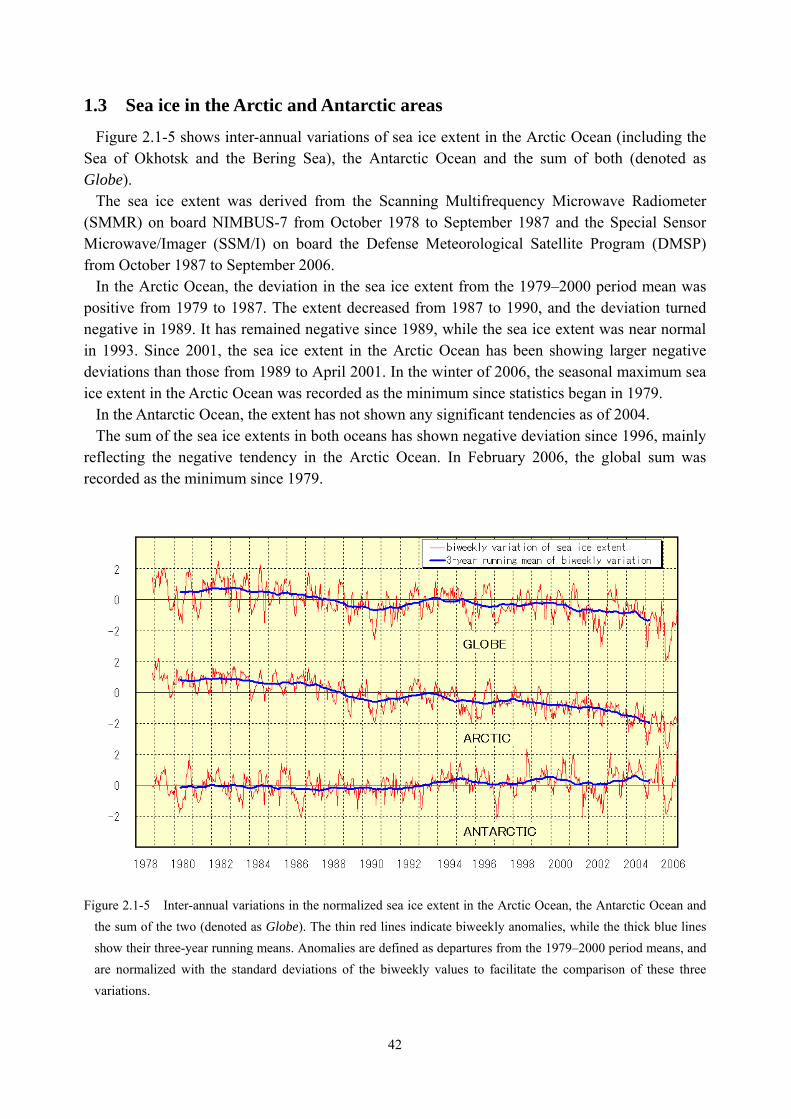
Figure 2.1-5 shows inter-annual variations of sea ice extent in the Arctic Ocean (including the Sea of Okhotsk and the Bering Sea), the Antarctic Ocean and the sum of both (denoted as Globe).

The sea ice extent was derived from the Scanning Multifrequency Microwave Radiometer (SMMR) on board NIMBUS-7 from October 1978 to September 1987 and the Special Sensor Microwave/Imager (SSM/I) on board the Defense Meteorological Satellite Program (DMSP) from October 1987 to September 2006.

In the Arctic Ocean, the deviation in the sea ice extent from the 1979–2000 period mean was positive from 1979 to 1987. The extent decreased from 1987 to 1990, and the deviation turned negative in 1989. It has remained negative since 1989, while the sea ice extent was near normal in 1993. Since 2001, the sea ice extent in the Arctic Ocean has been showing larger negative deviations than those from 1989 to April 2001. In the winter of 2006, the seasonal maximum sea ice extent in the Arctic Ocean was recorded as the minimum since statistics began in 1979.

In the Antarctic Ocean, the extent has not shown any significant tendencies as of 2004. The sum of the sea ice extents in both oceans has shown negative deviation since 1996, mainly

reflecting the negative tendency in the Arctic Ocean. In February 2006, the global sum was recorded as the minimum since 1979.

Figure 2.1-5 Inter-annual variations in the normalized sea ice extent in the Arctic Ocean, the Antarctic Ocean and

the sum of the two (denoted as Globe). The thin red lines indicate biweekly anomalies, while the thick blue lines show their three-year running means. Anomalies are defined as departures from the 1979–2000 period means, and are normalized with the standard deviations of the biweekly values to facilitate the comparison of these three variations.

43

2 The western North Pacific and the seas adjacent to Japan

2.1 Sea surface temperature and ocean currents in the western North Pacific

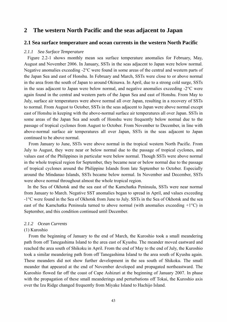
2.1.1 Sea Surface Temperature Figure 2.2-1 shows monthly mean sea surface temperature anomalies for February, May,

August and November 2006. In January, SSTs in the seas adjacent to Japan were below normal. Negative anomalies exceeding -2°C were found in some areas of the central and western parts of the Japan Sea and east of Honshu. In February and March, SSTs were close to or above normal in the area from the south of Japan to around Okinawa. In April, due to a strong cold surge, SSTs in the seas adjacent to Japan were below normal, and negative anomalies exceeding -2°C were again found in the central and western parts of the Japan Sea and east of Honshu. From May to July, surface air temperatures were above normal all over Japan, resulting in a recovery of SSTs to normal. From August to October, SSTs in the seas adjacent to Japan were above normal except east of Honshu in keeping with the above-normal surface air temperatures all over Japan. SSTs in some areas of the Japan Sea and south of Honshu were frequently below normal due to the passage of tropical cyclones from August to October. From November to December, in line with above-normal surface air temperatures all over Japan, SSTs in the seas adjacent to Japan continued to be above normal.

From January to June, SSTs were above normal in the tropical western North Pacific. From July to August, they were near or below normal due to the passage of tropical cyclones, and values east of the Philippines in particular were below normal. Though SSTs were above normal in the whole tropical region for September, they became near or below normal due to the passage of tropical cyclones around the Philippine Islands from late September to October. Especially around the Mindanao Islands, SSTs became below normal. In November and December, SSTs were above normal throughout almost the whole tropical region.

In the Sea of Okhotsk and the sea east of the Kamchatka Peninsula, SSTs were near normal from January to March. Negative SST anomalies began to spread in April, and values exceeding -1°C were found in the Sea of Okhotsk from June to July. SSTs in the Sea of Okhotsk and the sea east of the Kamchatka Peninsula turned to above normal (with anomalies exceeding +1°C) in September, and this condition continued until December. 2.1.2 Ocean Currents (1) Kuroshio

From the beginning of January to the end of March, the Kuroshio took a small meandering path from off Tanegashima Island to the area east of Kyushu. The meander moved eastward and reached the area south of Shikoku in April. From the end of May to the end of July, the Kuroshio took a similar meandering path from off Tanegashima Island to the area south of Kyushu again. These meanders did not show further development in the sea south of Shikoku. The small meander that appeared at the end of November developed and propagated northeastward. The Kuroshio flowed far off the coast of Cape Ashizuri at the beginning of January 2007. In phase with the propagation of these small meanderings and perturbations off Tokai, the Kuroshio axis over the Izu Ridge changed frequently from Miyake Island to Hachijo Island.

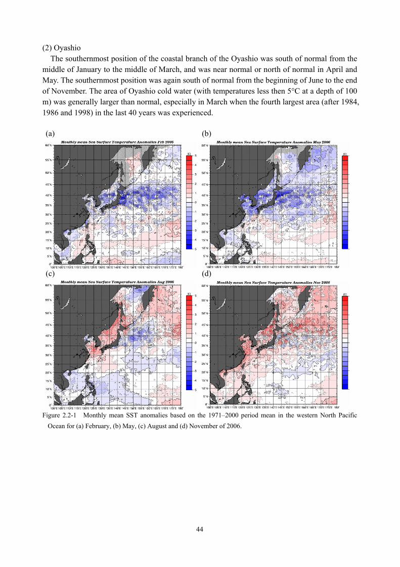
44

(2) Oyashio The southernmost position of the coastal branch of the Oyashio was south of normal from the

middle of January to the middle of March, and was near normal or north of normal in April and May. The southernmost position was again south of normal from the beginning of June to the end of November. The area of Oyashio cold water (with temperatures less then 5°C at a depth of 100 m) was generally larger than normal, especially in March when the fourth largest area (after 1984, 1986 and 1998) in the last 40 years was experienced. (a) (b)

(c) (d)

Figure 2.2-1 Monthly mean SST anomalies based on the 1971–2000 period mean in the western North Pacific Ocean for (a) February, (b) May, (c) August and (d) November of 2006.

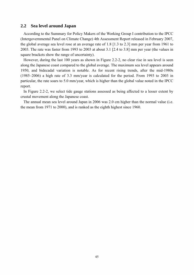
45

2.2 Sea level around Japan

According to the Summary for Policy Makers of the Working Group I contribution to the IPCC (Intergovernmental Panel on Climate Change) 4th Assessment Report released in February 2007, the global average sea level rose at an average rate of 1.8 [1.3 to 2.3] mm per year from 1961 to 2003. The rate was faster from 1993 to 2003 at about 3.1 [2.4 to 3.8] mm per year (the values in square brackets show the range of uncertainty).

However, during the last 100 years as shown in Figure 2.2-2, no clear rise in sea level is seen along the Japanese coast compared to the global average. The maximum sea level appears around 1950, and bidecadal variation is notable. As for recent rising trends, after the mid-1980s (1985–2006) a high rate of 3.3 mm/year is calculated for the period. From 1993 to 2003 in particular, the rate soars to 5.0 mm/year, which is higher than the global value noted in the IPCC report.

In Figure 2.2-2, we select tide gauge stations assessed as being affected to a lesser extent by crustal movement along the Japanese coast.

The annual mean sea level around Japan in 2006 was 2.0 cm higher than the normal value (i.e. the mean from 1971 to 2000), and is ranked as the eighth highest since 1960.

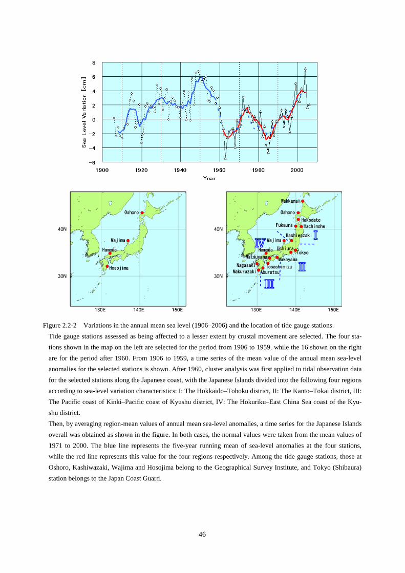
46

Figure 2.2-2 Variations in the annual mean sea level (1906–2006) and the location of tide gauge stations.

Tide gauge stations assessed as being affected to a lesser extent by crustal movement are selected. The four sta-tions shown in the map on the left are selected for the period from 1906 to 1959, while the 16 shown on the right are for the period after 1960. From 1906 to 1959, a time series of the mean value of the annual mean sea-level anomalies for the selected stations is shown. After 1960, cluster analysis was first applied to tidal observation data for the selected stations along the Japanese coast, with the Japanese Islands divided into the following four regions according to sea-level variation characteristics: I: The Hokkaido–Tohoku district, II: The Kanto–Tokai district, III: The Pacific coast of Kinki–Pacific coast of Kyushu district, IV: The Hokuriku–East China Sea coast of the Kyu-shu district. Then, by averaging region-mean values of annual mean sea-level anomalies, a time series for the Japanese Islands overall was obtained as shown in the figure. In both cases, the normal values were taken from the mean values of 1971 to 2000. The blue line represents the five-year running mean of sea-level anomalies at the four stations, while the red line represents this value for the four regions respectively. Among the tide gauge stations, those at Oshoro, Kashiwazaki, Wajima and Hosojima belong to the Geographical Survey Institute, and Tokyo (Shibaura) station belongs to the Japan Coast Guard.

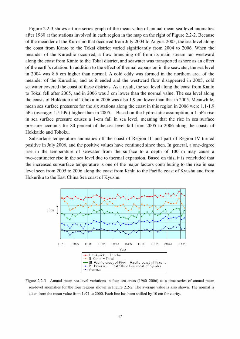
47

Figure 2.2-3 shows a time-series graph of the mean value of annual mean sea-level anomalies after 1960 at the stations involved in each region in the map on the right of Figure 2.2-2. Because of the meander of the Kuroshio that occurred from July 2004 to August 2005, the sea level along the coast from Kanto to the Tokai district varied significantly from 2004 to 2006. When the meander of the Kuroshio occurred, a flow branching off from its main stream ran westward along the coast from Kanto to the Tokai district, and seawater was transported ashore as an effect of the earth’s rotation. In addition to the effect of thermal expansion in the seawater, the sea level in 2004 was 8.6 cm higher than normal. A cold eddy was formed in the northern area of the meander of the Kuroshio, and as it ended and the westward flow disappeared in 2005, cold seawater covered the coast of these districts. As a result, the sea level along the coast from Kanto to Tokai fell after 2005, and in 2006 was 3 cm lower than the normal value. The sea level along the coasts of Hokkaido and Tohoku in 2006 was also 1.9 cm lower than that in 2005. Meanwhile, mean sea surface pressures for the six stations along the coast in this region in 2006 were 1.1-1.9 hPa (average: 1.5 hPa) higher than in 2005. Based on the hydrostatic assumption, a 1-hPa rise in sea surface pressure causes a 1-cm fall in sea level, meaning that the rise in sea surface pressure accounts for 80 percent of the sea-level fall from 2005 to 2006 along the coasts of Hokkaido and Tohoku.

Subsurface temperature anomalies off the coast of Region III and part of Region IV turned positive in July 2006, and the positive values have continued since then. In general, a one-degree rise in the temperature of seawater from the surface to a depth of 100 m may cause a two-centimeter rise in the sea level due to thermal expansion. Based on this, it is concluded that the increased subsurface temperature is one of the major factors contributing to the rise in sea level seen from 2005 to 2006 along the coast from Kinki to the Pacific coast of Kyushu and from Hokuriku to the East China Sea coast of Kyushu.

Figure 2.2-3 Annual mean sea-level variations in four sea areas (1960–2006) as a time series of annual mean

sea-level anomalies for the four regions shown in Figure 2.2-2. The average value is also shown. The normal is taken from the mean value from 1971 to 2000. Each line has been shifted by 10 cm for clarity.

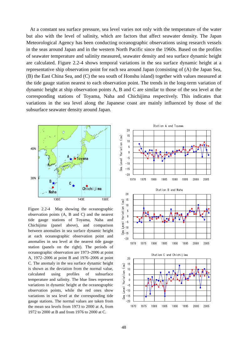
48

At a constant sea surface pressure, sea level varies not only with the temperature of the water but also with the level of salinity, which are factors that affect seawater density. The Japan Meteorological Agency has been conducting oceanographic observations using research vessels in the seas around Japan and in the western North Pacific since the 1960s. Based on the profiles of seawater temperature and salinity measured, seawater density and sea surface dynamic height are calculated. Figure 2.2-4 shows temporal variations in the sea surface dynamic height at a representative ship observation point for each sea around Japan (consisting of (A) the Japan Sea, (B) the East China Sea, and (C) the sea south of Honshu island) together with values measured at the tide gauge station nearest to each observation point. The trends in the long-term variation of dynamic height at ship observation points A, B and C are similar to those of the sea level at the corresponding stations of Toyama, Naha and Chichijima respectively. This indicates that variations in the sea level along the Japanese coast are mainly influenced by those of the subsurface seawater density around Japan.

Figure 2.2-4 Map showing the oceanographic observation points (A, B and C) and the nearest tide gauge stations of Toyama, Naha and Chichijima (panel above), and comparison between anomalies in sea surface dynamic height at each oceanographic observation point and anomalies in sea level at the nearest tide gauge station (panels on the right). The periods of oceanographic observation are 1973–2006 at point A, 1972–2006 at point B and 1976–2006 at point C. The anomaly in the sea surface dynamic height is shown as the deviation from the normal value, calculated using profiles of subsurface temperature and salinity. The blue lines represent variations in dynamic height at the oceanographic observation points, while the red ones show variations in sea level at the corresponding tide gauge stations. The normal values are taken from the mean sea levels from 1973 to 2000 at A, from 1972 to 2000 at B and from 1976 to 2000 at C.

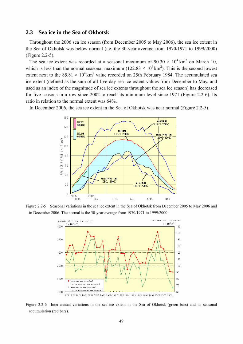
49

2.3 Sea ice in the Sea of Okhotsk

Throughout the 2006 sea ice season (from December 2005 to May 2006), the sea ice extent in the Sea of Okhotsk was below normal (i.e. the 30-year average from 1970/1971 to 1999/2000) (Figure 2.2-5).

The sea ice extent was recorded at a seasonal maximum of 90.30 × 104 km2 on March 10, which is less than the normal seasonal maximum (122.83 × 104 km2). This is the second lowest extent next to the 85.81 × 104 km2 value recorded on 25th February 1984. The accumulated sea ice extent (defined as the sum of all five-day sea ice extent values from December to May, and used as an index of the magnitude of sea ice extents throughout the sea ice season) has decreased for five seasons in a row since 2002 to reach its minimum level since 1971 (Figure 2.2-6). Its ratio in relation to the normal extent was 64%.

In December 2006, the sea ice extent in the Sea of Okhotsk was near normal (Figure 2.2-5).

Figure 2.2-5 Seasonal variations in the sea ice extent in the Sea of Okhotsk from December 2005 to May 2006 and

in December 2006. The normal is the 30-year average from 1970/1971 to 1999/2000.

Figure 2.2-6 Inter-annual variations in the sea ice extent in the Sea of Okhotsk (green bars) and its seasonal

accumulation (red bars).

50

2.4 Marine pollution in the western North Pacific

Activities based on an international framework are essential toward the prevention of marine pollution. In Japan, the Law Relating to the Prevention of Marine Pollution and Maritime Disaster took effect in 1971 against a background of discussion on the adoption of the Convention on the Prevention of Marine Pollution by Dumping of Wastes and other Matter (a.k.a. the London Dumping Convention, or LDC) and the International Convention for the Prevention of Pollution from Ships (a.k.a. the MARPOL73/78 Convention). For the purposes of preventing marine pollution and preserving the marine environment based on this law, the Japan Meteorological Agency (JMA) has been monitoring background marine pollution since 1972. 2.4.1 Floating pollutants (plastics)

Floating pollutants are counted by continuous observation from the bridges of research vessels during the daytime. When observers find a floating pollutant, they record its location and type, and “NIL” is recorded if no pollutant is found. JMA pays particular attention to plastics among floating pollutants. Plastics are categorized into the four types of polystyrene foams, fishing gear, plastic film and other plastics. The data observed are arranged by adding together the floating plastics counted along cruise tracks of 100 km each.

Figure 2.2-7 shows the distribution of floating plastics in the four seasons of 2006. A black circle whose size corresponds to the number of plastics found is plotted on the ship’s position at noon of each day (“+” symbols denote “NIL”). In 2006, the total track length was 64,705 km, and the total number of observed floating plastics was 3,447. In some parts of the sea adjacent to Japan, more than 50 pieces/100 km were found from spring to autumn of 2006. 10-20 pieces/100 km were also found in the areas around 30°N, south of the Kuroshio and the Kuroshio Extension. In the areas south of 20°N, only several pieces per 100 km were found throughout all seasons.

Figure 2.2-8 shows the observed amount of floating plastic (in pieces/100 km) of the four categories in each area. In 2006, the observed amount averaged over the whole track was 5.4 pieces/100 km, which is almost the same as the 2005 level of 5.2 pieces/100 km. In the Japan Sea, the amount of floating plastic observed in 2006 was 12.6 pieces/100 km, slightly up from the 10.5 pieces/100 km value of 2005. On the other hand, in the East China Sea, the figure for 2006 was 7.2 pieces/100 km, down from 10.0 pieces/100 km in 2005. Polystyrene foams (representing 53% of the average number over all tracks) and fishing gear (16%) accounted for a large part of the categories of observed floating plastics.

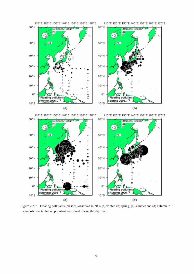
51

Figure 2.2-7 Floating pollutants (plastics) observed in 2006 (a) winter, (b) spring, (c) summer and (d) autumn. “+”

symbols denote that no pollutant was found during the daytime.

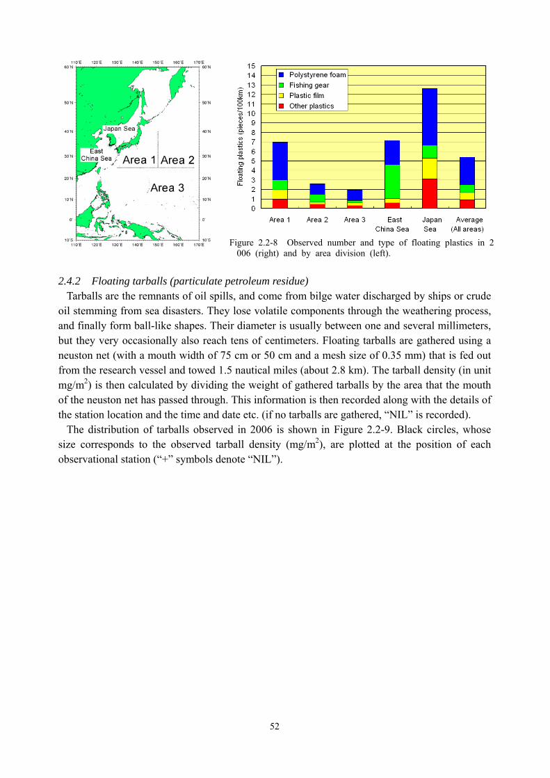
52

Figure 2.2-8 Observed number and type of floating plastics in 2

006 (right) and by area division (left). 2.4.2 Floating tarballs (particulate petroleum residue)

Tarballs are the remnants of oil spills, and come from bilge water discharged by ships or crude oil stemming from sea disasters. They lose volatile components through the weathering process, and finally form ball-like shapes. Their diameter is usually between one and several millimeters, but they very occasionally also reach tens of centimeters. Floating tarballs are gathered using a neuston net (with a mouth width of 75 cm or 50 cm and a mesh size of 0.35 mm) that is fed out from the research vessel and towed 1.5 nautical miles (about 2.8 km). The tarball density (in unit mg/m2) is then calculated by dividing the weight of gathered tarballs by the area that the mouth of the neuston net has passed through. This information is then recorded along with the details of the station location and the time and date etc. (if no tarballs are gathered, “NIL” is recorded).

The distribution of tarballs observed in 2006 is shown in Figure 2.2-9. Black circles, whose size corresponds to the observed tarball density (mg/m2), are plotted at the position of each observational station (“+” symbols denote “NIL”).

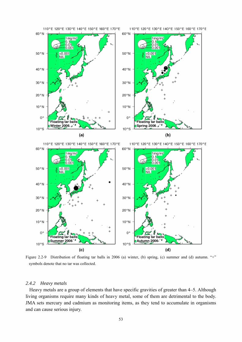
53

Figure 2.2-9 Distribution of floating tar balls in 2006 (a) winter, (b) spring, (c) summer and (d) autumn. “+”

symbols denote that no tar was collected.

2.4.2 Heavy metals Heavy metals are a group of elements that have specific gravities of greater than 4–5. Although

living organisms require many kinds of heavy metal, some of them are detrimental to the body. JMA sets mercury and cadmium as monitoring items, as they tend to accumulate in organisms and can cause serious injury.

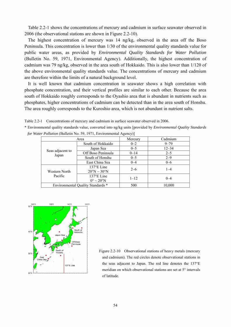
54

Table 2.2-1 shows the concentrations of mercury and cadmium in surface seawater observed in 2006 (the observational stations are shown in Figure 2.2-10).

The highest concentration of mercury was 14 ng/kg, observed in the area off the Boso Peninsula. This concentration is lower than 1/30 of the environmental quality standards value for public water areas, as provided by Environmental Quality Standards for Water Pollution (Bulletin No. 59, 1971, Environmental Agency). Additionally, the highest concentration of cadmium was 79 ng/kg, observed in the area south of Hokkaido. This is also lower than 1/120 of the above environmental quality standards value. The concentrations of mercury and cadmium are therefore within the limits of a natural background level.

It is well known that cadmium concentration in seawater shows a high correlation with phosphate concentration, and their vertical profiles are similar to each other. Because the area south of Hokkaido roughly corresponds to the Oyashio area that is abundant in nutrients such as phosphates, higher concentrations of cadmium can be detected than in the area south of Honshu. The area roughly corresponds to the Kuroshio area, which is not abundant in nutrient salts. Table 2.2-1 Concentrations of mercury and cadmium in surface seawater observed in 2006. * Environmental quality standards value, converted into ng/kg units [provided by Environmental Quality Standards

for Water Pollution (Bulletin No. 59, 1971, Environmental Agency)] Area Mercury Cadmium

South of Hokkaido 0–2 9–79 Japan Sea 0–5 12–34

Off Boso Peninsula 0–14 2–5 South of Honshu 0–5 2–9

Seas adjacent to Japan

East China Sea 0–4 0–6 137°E Line

20°N ~ 30°N 2–6 1–4 Western North Pacific 137°E Line

0° ~ 20°N 1–12 0–4

Environmental Quality Standards * 500 10,000

Figure 2.2-10 Observational stations of heavy metals (mercury and cadmium). The red circles denote observational stations in the seas adjacent to Japan. The red line denotes the 137°E meridian on which observational stations are set at 5° intervals of latitude.

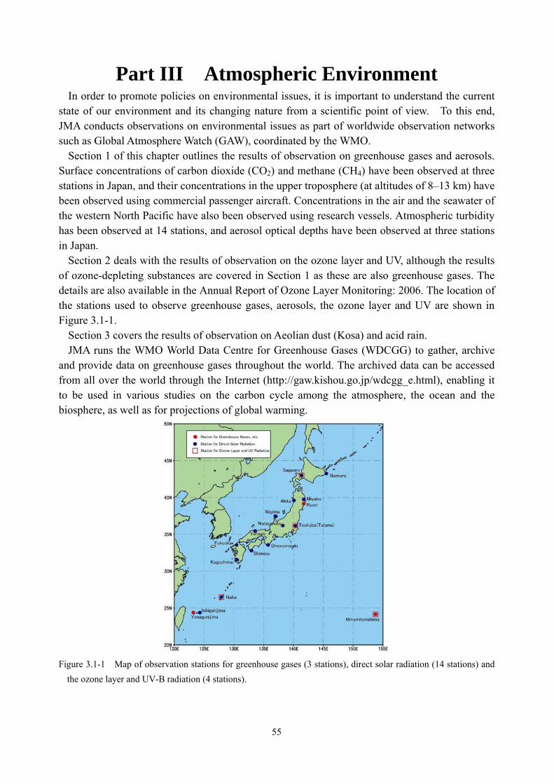
55

Part III Atmospheric Environment In order to promote policies on environmental issues, it is important to understand the current

state of our environment and its changing nature from a scientific point of view. To this end, JMA conducts observations on environmental issues as part of worldwide observation networks such as Global Atmosphere Watch (GAW), coordinated by the WMO.

Section 1 of this chapter outlines the results of observation on greenhouse gases and aerosols. Surface concentrations of carbon dioxide (CO2) and methane (CH4) have been observed at three stations in Japan, and their concentrations in the upper troposphere (at altitudes of 8–13 km) have been observed using commercial passenger aircraft. Concentrations in the air and the seawater of the western North Pacific have also been observed using research vessels. Atmospheric turbidity has been observed at 14 stations, and aerosol optical depths have been observed at three stations in Japan.

Section 2 deals with the results of observation on the ozone layer and UV, although the results of ozone-depleting substances are covered in Section 1 as these are also greenhouse gases. The details are also available in the Annual Report of Ozone Layer Monitoring: 2006. The location of the stations used to observe greenhouse gases, aerosols, the ozone layer and UV are shown in Figure 3.1-1.

Section 3 covers the results of observation on Aeolian dust (Kosa) and acid rain. JMA runs the WMO World Data Centre for Greenhouse Gases (WDCGG) to gather, archive

and provide data on greenhouse gases throughout the world. The archived data can be accessed from all over the world through the Internet (http://gaw.kishou.go.jp/wdcgg_e.html), enabling it to be used in various studies on the carbon cycle among the atmosphere, the ocean and the biosphere, as well as for projections of global warming.

Figure 3.1-1 Map of observation stations for greenhouse gases (3 stations), direct solar radiation (14 stations) and

the ozone layer and UV-B radiation (4 stations).

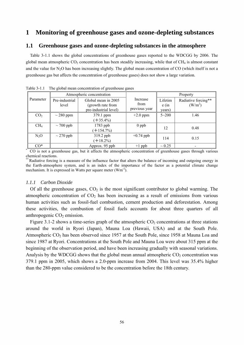
56

1 Monitoring of greenhouse gases and ozone-depleting substances

1.1 Greenhouse gases and ozone-depleting substances in the atmosphere Table 3-1.1 shows the global concentrations of greenhouse gases reported to the WDCGG by 2006. The

global mean atmospheric CO2 concentration has been steadily increasing, while that of CH4 is almost constant and the value for N2O has been increasing slightly. The global mean concentration of CO (which itself is not a greenhouse gas but affects the concentration of greenhouse gases) does not show a large variation. Table 3-1.1 The global mean concentration of greenhouse gases

Atmospheric concentration Property Parameter Pre-industrial

level Global mean in 2005

(growth rate from pre-industrial level)

Increase

from previous year

Lifetime (in

years)

Radiative forcing** (W/m2)

CO2 ~ 280 ppm 379.1 ppm (＋35.4%)

+2.0 ppm 5~200 1.46

CH4 ~ 700 ppb 1783 ppb (＋154.7%)

0 ppb 12 0.48

N2O ~ 270 ppb 319.2 ppb (＋18.2%)

+0.74 ppb 114 0.15

CO* Approx. 95 ppb +1 ppb ~ 0.25 - * CO is not a greenhouse gas, but it affects the atmospheric concentration of greenhouse gases through various chemical reactions. ** Radiative forcing is a measure of the influence factor that alters the balance of incoming and outgoing energy in the Earth-atmosphere system, and is an index of the importance of the factor as a potential climate change mechanism. It is expressed in Watts per square meter (Wm-2). 1.1.1 Carbon Dioxide

Of all the greenhouse gases, CO2 is the most significant contributor to global warming. The atmospheric concentration of CO2 has been increasing as a result of emissions from various human activities such as fossil-fuel combustion, cement production and deforestation. Among these activities, the combustion of fossil fuels accounts for about three quarters of all anthropogenic CO2 emission.

Figure 3.1-2 shows a time-series graph of the atmospheric CO2 concentrations at three stations around the world in Ryori (Japan), Mauna Loa (Hawaii, USA) and at the South Pole. Atmospheric CO2 has been observed since 1957 at the South Pole, since 1958 at Mauna Loa and since 1987 at Ryori. Concentrations at the South Pole and Mauna Loa were about 315 ppm at the beginning of the observation period, and have been increasing gradually with seasonal variations. Analysis by the WDCGG shows that the global mean annual atmospheric CO2 concentration was 379.1 ppm in 2005, which shows a 2.0-ppm increase from 2004. This level was 35.4% higher than the 280-ppm value considered to be the concentration before the 18th century.

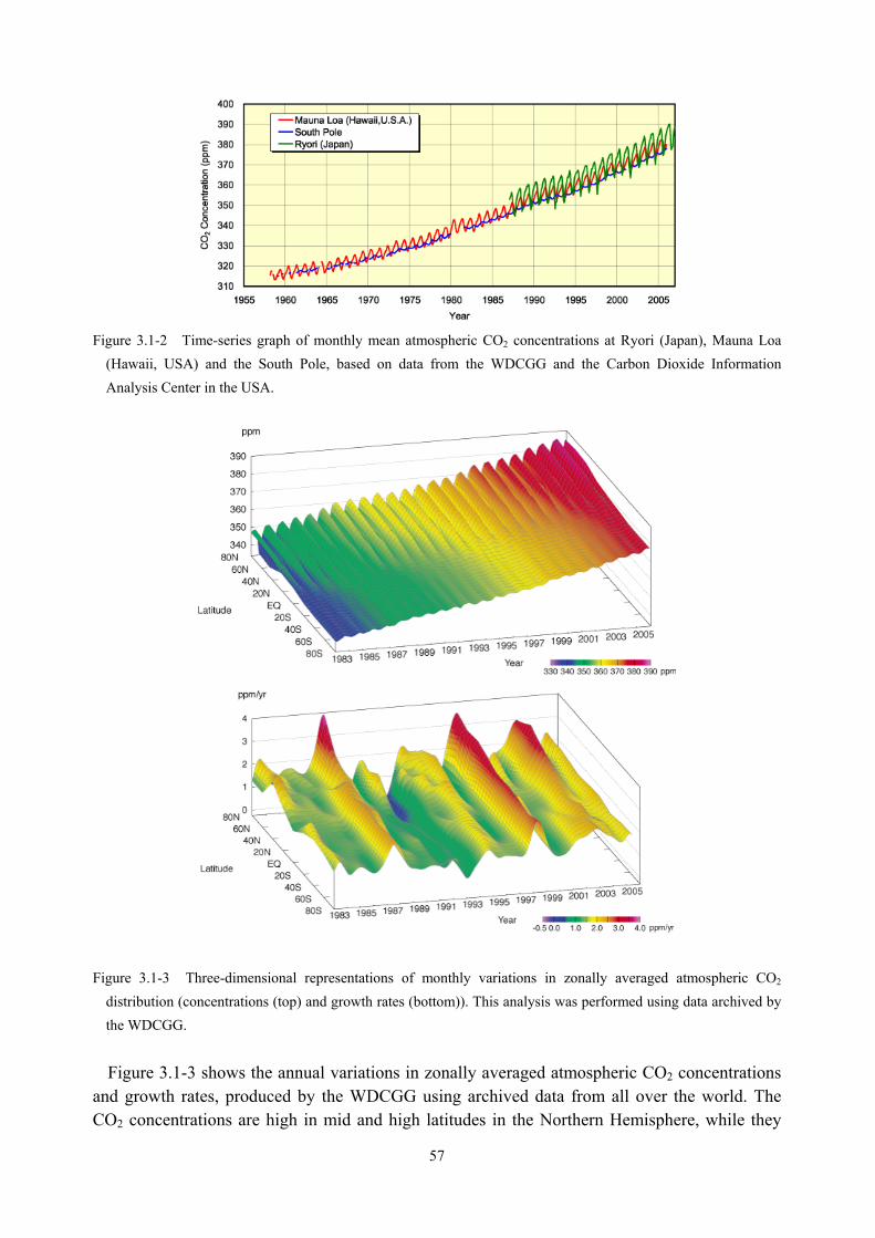
57

Figure 3.1-2 Time-series graph of monthly mean atmospheric CO2 concentrations at Ryori (Japan), Mauna Loa

(Hawaii, USA) and the South Pole, based on data from the WDCGG and the Carbon Dioxide Information Analysis Center in the USA.

Figure 3.1-3 Three-dimensional representations of monthly variations in zonally averaged atmospheric CO2 distribution (concentrations (top) and growth rates (bottom)). This analysis was performed using data archived by the WDCGG.

Figure 3.1-3 shows the annual variations in zonally averaged atmospheric CO2 concentrations

and growth rates, produced by the WDCGG using archived data from all over the world. The CO2 concentrations are high in mid and high latitudes in the Northern Hemisphere, while they

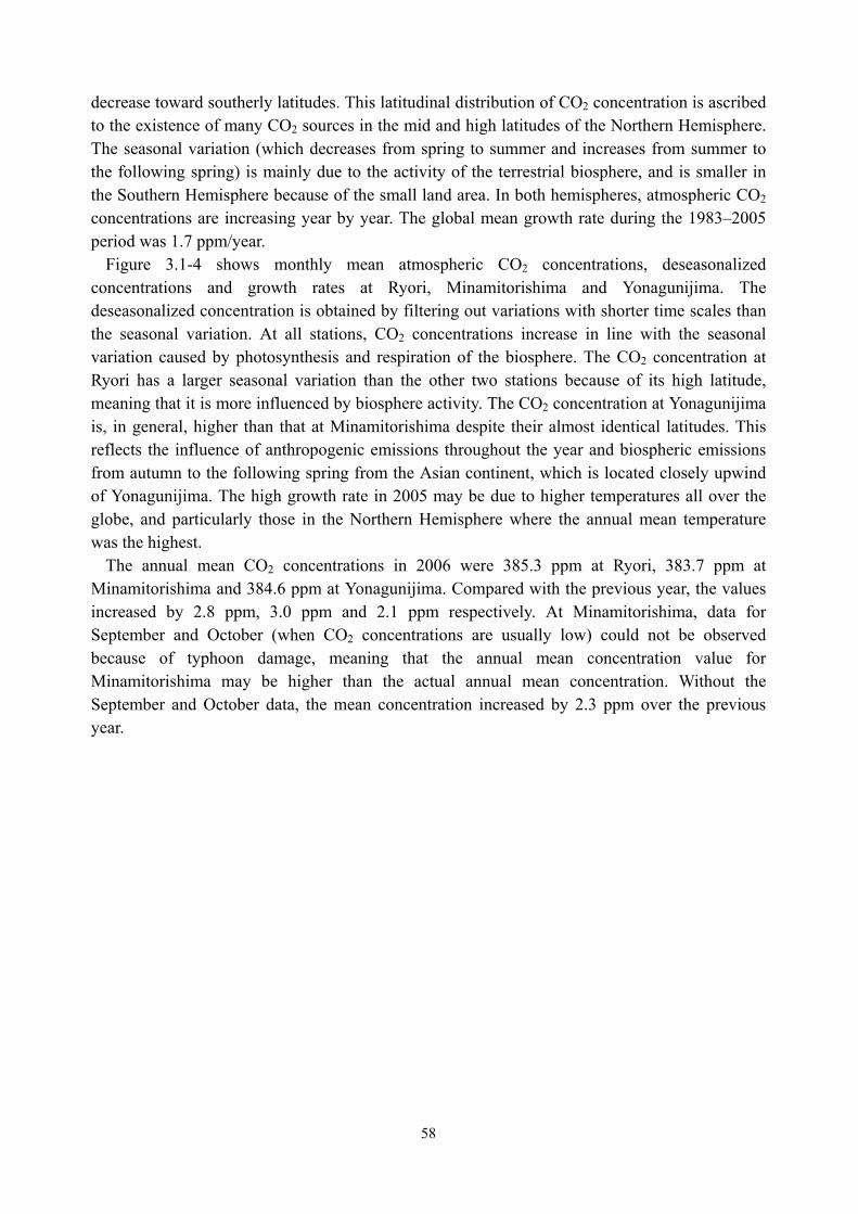
58

decrease toward southerly latitudes. This latitudinal distribution of CO2 concentration is ascribed to the existence of many CO2 sources in the mid and high latitudes of the Northern Hemisphere. The seasonal variation (which decreases from spring to summer and increases from summer to the following spring) is mainly due to the activity of the terrestrial biosphere, and is smaller in the Southern Hemisphere because of the small land area. In both hemispheres, atmospheric CO2 concentrations are increasing year by year. The global mean growth rate during the 1983–2005 period was 1.7 ppm/year.

Figure 3.1-4 shows monthly mean atmospheric CO2 concentrations, deseasonalized concentrations and growth rates at Ryori, Minamitorishima and Yonagunijima. The deseasonalized concentration is obtained by filtering out variations with shorter time scales than the seasonal variation. At all stations, CO2 concentrations increase in line with the seasonal variation caused by photosynthesis and respiration of the biosphere. The CO2 concentration at Ryori has a larger seasonal variation than the other two stations because of its high latitude, meaning that it is more influenced by biosphere activity. The CO2 concentration at Yonagunijima is, in general, higher than that at Minamitorishima despite their almost identical latitudes. This reflects the influence of anthropogenic emissions throughout the year and biospheric emissions from autumn to the following spring from the Asian continent, which is located closely upwind of Yonagunijima. The high growth rate in 2005 may be due to higher temperatures all over the globe, and particularly those in the Northern Hemisphere where the annual mean temperature was the highest.

The annual mean CO2 concentrations in 2006 were 385.3 ppm at Ryori, 383.7 ppm at Minamitorishima and 384.6 ppm at Yonagunijima. Compared with the previous year, the values increased by 2.8 ppm, 3.0 ppm and 2.1 ppm respectively. At Minamitorishima, data for September and October (when CO2 concentrations are usually low) could not be observed because of typhoon damage, meaning that the annual mean concentration value for Minamitorishima may be higher than the actual annual mean concentration. Without the September and October data, the mean concentration increased by 2.3 ppm over the previous year.

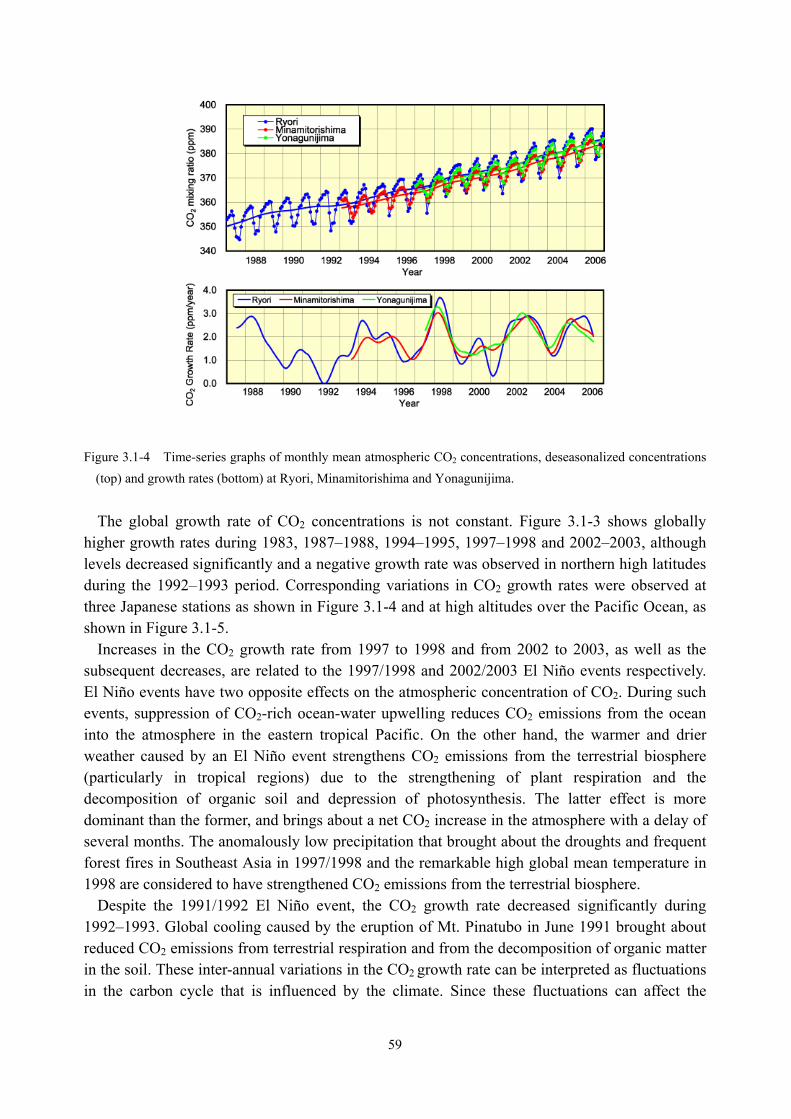
59

Figure 3.1-4 Time-series graphs of monthly mean atmospheric CO2 concentrations, deseasonalized concentrations

(top) and growth rates (bottom) at Ryori, Minamitorishima and Yonagunijima.

The global growth rate of CO2 concentrations is not constant. Figure 3.1-3 shows globally

higher growth rates during 1983, 1987–1988, 1994–1995, 1997–1998 and 2002–2003, although levels decreased significantly and a negative growth rate was observed in northern high latitudes during the 1992–1993 period. Corresponding variations in CO2 growth rates were observed at three Japanese stations as shown in Figure 3.1-4 and at high altitudes over the Pacific Ocean, as shown in Figure 3.1-5.

Increases in the CO2 growth rate from 1997 to 1998 and from 2002 to 2003, as well as the subsequent decreases, are related to the 1997/1998 and 2002/2003 El Niño events respectively. El Niño events have two opposite effects on the atmospheric concentration of CO2. During such events, suppression of CO2-rich ocean-water upwelling reduces CO2 emissions from the ocean into the atmosphere in the eastern tropical Pacific. On the other hand, the warmer and drier weather caused by an El Niño event strengthens CO2 emissions from the terrestrial biosphere (particularly in tropical regions) due to the strengthening of plant respiration and the decomposition of organic soil and depression of photosynthesis. The latter effect is more dominant than the former, and brings about a net CO2 increase in the atmosphere with a delay of several months. The anomalously low precipitation that brought about the droughts and frequent forest fires in Southeast Asia in 1997/1998 and the remarkable high global mean temperature in 1998 are considered to have strengthened CO2 emissions from the terrestrial biosphere.

Despite the 1991/1992 El Niño event, the CO2 growth rate decreased significantly during 1992–1993. Global cooling caused by the eruption of Mt. Pinatubo in June 1991 brought about reduced CO2 emissions from terrestrial respiration and from the decomposition of organic matter in the soil. These inter-annual variations in the CO2 growth rate can be interpreted as fluctuations in the carbon cycle that is influenced by the climate. Since these fluctuations can affect the

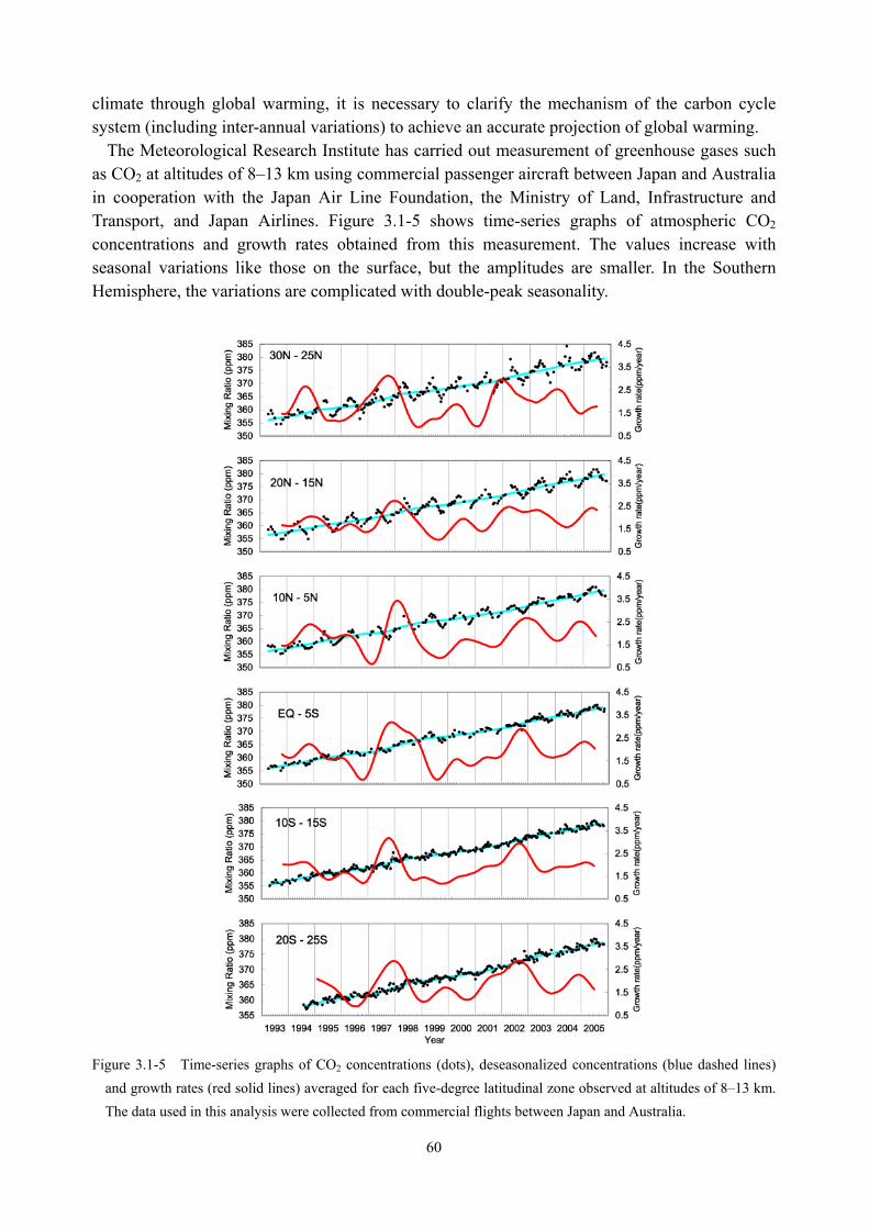
60

climate through global warming, it is necessary to clarify the mechanism of the carbon cycle system (including inter-annual variations) to achieve an accurate projection of global warming.

The Meteorological Research Institute has carried out measurement of greenhouse gases such as CO2 at altitudes of 8–13 km using commercial passenger aircraft between Japan and Australia in cooperation with the Japan Air Line Foundation, the Ministry of Land, Infrastructure and Transport, and Japan Airlines. Figure 3.1-5 shows time-series graphs of atmospheric CO2 concentrations and growth rates obtained from this measurement. The values increase with seasonal variations like those on the surface, but the amplitudes are smaller. In the Southern Hemisphere, the variations are complicated with double-peak seasonality.

Figure 3.1-5 Time-series graphs of CO2 concentrations (dots), deseasonalized concentrations (blue dashed lines)

and growth rates (red solid lines) averaged for each five-degree latitudinal zone observed at altitudes of 8–13 km. The data used in this analysis were collected from commercial flights between Japan and Australia.

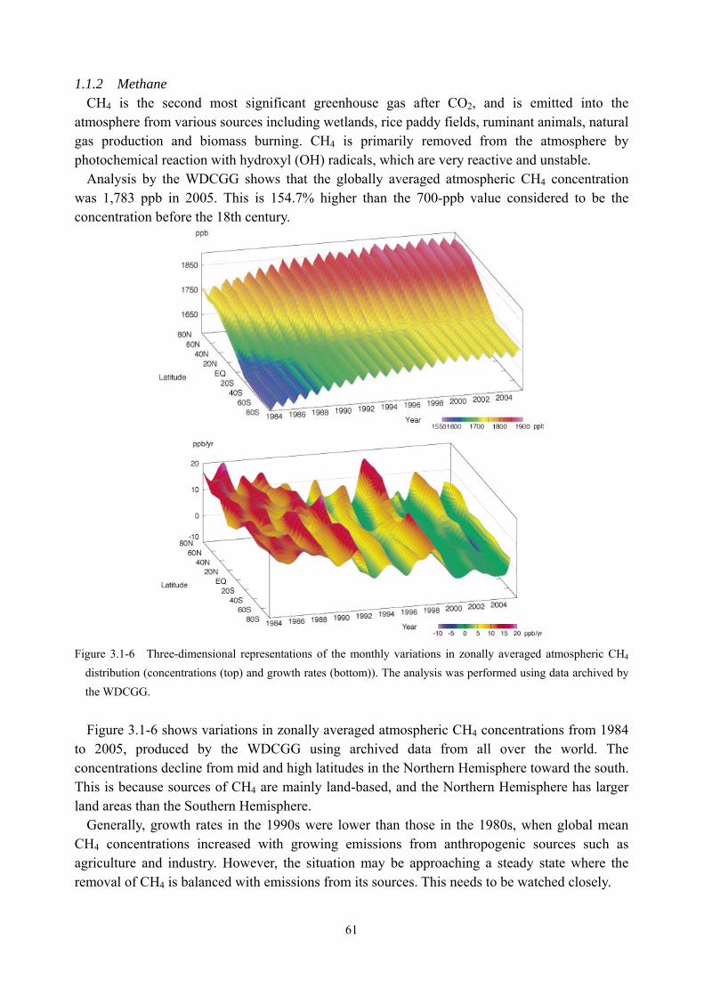
61

1.1.2 Methane CH4 is the second most significant greenhouse gas after CO2, and is emitted into the

atmosphere from various sources including wetlands, rice paddy fields, ruminant animals, natural gas production and biomass burning. CH4 is primarily removed from the atmosphere by photochemical reaction with hydroxyl (OH) radicals, which are very reactive and unstable.

Analysis by the WDCGG shows that the globally averaged atmospheric CH4 concentration was 1,783 ppb in 2005. This is 154.7% higher than the 700-ppb value considered to be the concentration before the 18th century.

Figure 3.1-6 Three-dimensional representations of the monthly variations in zonally averaged atmospheric CH4

distribution (concentrations (top) and growth rates (bottom)). The analysis was performed using data archived by the WDCGG.

Figure 3.1-6 shows variations in zonally averaged atmospheric CH4 concentrations from 1984

to 2005, produced by the WDCGG using archived data from all over the world. The concentrations decline from mid and high latitudes in the Northern Hemisphere toward the south. This is because sources of CH4 are mainly land-based, and the Northern Hemisphere has larger land areas than the Southern Hemisphere.

Generally, growth rates in the 1990s were lower than those in the 1980s, when global mean CH4 concentrations increased with growing emissions from anthropogenic sources such as agriculture and industry. However, the situation may be approaching a steady state where the removal of CH4 is balanced with emissions from its sources. This needs to be watched closely.

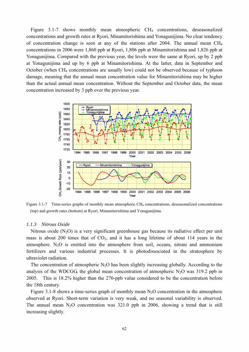
62

Figure 3.1-7 shows monthly mean atmospheric CH4 concentrations, deseasonalized concentrations and growth rates at Ryori, Minamitorishima and Yonagunijima. No clear tendency of concentration change is seen at any of the stations after 2004. The annual mean CH4 concentrations in 2006 were 1,860 ppb at Ryori, 1,806 ppb at Minamitorishima and 1,826 ppb at Yonagunijima. Compared with the previous year, the levels were the same at Ryori, up by 2 ppb at Yonagunijima and up by 6 ppb at Minamitorishima. At the latter, data in September and October (when CH4 concentrations are usually low) could not be observed because of typhoon damage, meaning that the annual mean concentration value for Minamitorishima may be higher than the actual annual mean concentration. Without the September and October data, the mean concentration increased by 3 ppb over the previous year.

Figure 3.1-7 Time-series graphs of monthly mean atmospheric CH4 concentrations, deseasonalized concentrations

(top) and growth rates (bottom) at Ryori, Minamitorishima and Yonagunijima. 1.1.3 Nitrous Oxide

Nitrous oxide (N2O) is a very significant greenhouse gas because its radiative effect per unit mass is about 200 times that of CO2, and it has a long lifetime of about 114 years in the atmosphere. N2O is emitted into the atmosphere from soil, oceans, nitrate and ammonium fertilizers and various industrial processes. It is photodissociated in the stratosphere by ultraviolet radiation.

The concentration of atmospheric N2O has been slightly increasing globally. According to the analysis of the WDCGG, the global mean concentration of atmospheric N2O was 319.2 ppb in 2005. This is 18.2% higher than the 270-ppb value considered to be the concentration before the 18th century.

Figure 3.1-8 shows a time-series graph of monthly mean N2O concentration in the atmosphere observed at Ryori. Short-term variation is very weak, and no seasonal variability is observed. The annual mean N2O concentration was 321.0 ppb in 2006, showing a trend that is still increasing slightly.

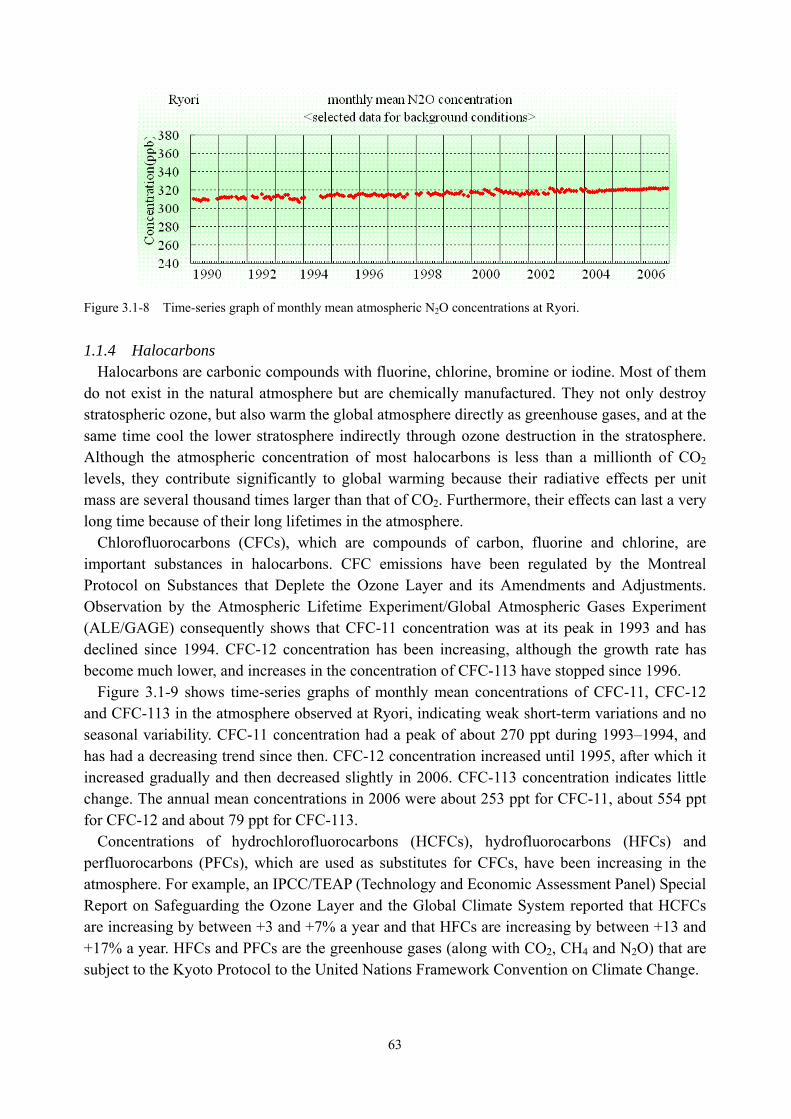
63

Figure 3.1-8 Time-series graph of monthly mean atmospheric N2O concentrations at Ryori.

1.1.4 Halocarbons

Halocarbons are carbonic compounds with fluorine, chlorine, bromine or iodine. Most of them do not exist in the natural atmosphere but are chemically manufactured. They not only destroy stratospheric ozone, but also warm the global atmosphere directly as greenhouse gases, and at the same time cool the lower stratosphere indirectly through ozone destruction in the stratosphere. Although the atmospheric concentration of most halocarbons is less than a millionth of CO2 levels, they contribute significantly to global warming because their radiative effects per unit mass are several thousand times larger than that of CO2. Furthermore, their effects can last a very long time because of their long lifetimes in the atmosphere.

Chlorofluorocarbons (CFCs), which are compounds of carbon, fluorine and chlorine, are important substances in halocarbons. CFC emissions have been regulated by the Montreal Protocol on Substances that Deplete the Ozone Layer and its Amendments and Adjustments. Observation by the Atmospheric Lifetime Experiment/Global Atmospheric Gases Experiment (ALE/GAGE) consequently shows that CFC-11 concentration was at its peak in 1993 and has declined since 1994. CFC-12 concentration has been increasing, although the growth rate has become much lower, and increases in the concentration of CFC-113 have stopped since 1996.

Figure 3.1-9 shows time-series graphs of monthly mean concentrations of CFC-11, CFC-12 and CFC-113 in the atmosphere observed at Ryori, indicating weak short-term variations and no seasonal variability. CFC-11 concentration had a peak of about 270 ppt during 1993–1994, and has had a decreasing trend since then. CFC-12 concentration increased until 1995, after which it increased gradually and then decreased slightly in 2006. CFC-113 concentration indicates little change. The annual mean concentrations in 2006 were about 253 ppt for CFC-11, about 554 ppt for CFC-12 and about 79 ppt for CFC-113.

Concentrations of hydrochlorofluorocarbons (HCFCs), hydrofluorocarbons (HFCs) and perfluorocarbons (PFCs), which are used as substitutes for CFCs, have been increasing in the atmosphere. For example, an IPCC/TEAP (Technology and Economic Assessment Panel) Special Report on Safeguarding the Ozone Layer and the Global Climate System reported that HCFCs are increasing by between +3 and +7% a year and that HFCs are increasing by between +13 and +17% a year. HFCs and PFCs are the greenhouse gases (along with CO2, CH4 and N2O) that are subject to the Kyoto Protocol to the United Nations Framework Convention on Climate Change.

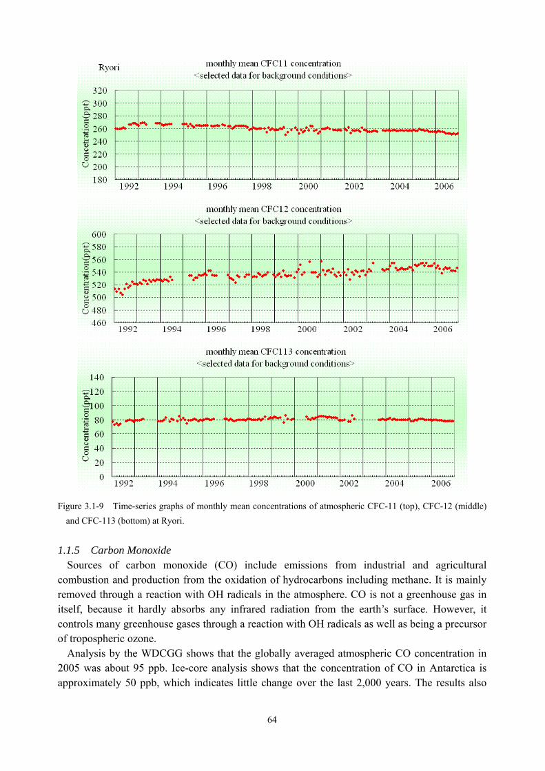
64

Figure 3.1-9 Time-series graphs of monthly mean concentrations of atmospheric CFC-11 (top), CFC-12 (middle)

and CFC-113 (bottom) at Ryori.

1.1.5 Carbon Monoxide

Sources of carbon monoxide (CO) include emissions from industrial and agricultural combustion and production from the oxidation of hydrocarbons including methane. It is mainly removed through a reaction with OH radicals in the atmosphere. CO is not a greenhouse gas in itself, because it hardly absorbs any infrared radiation from the earth’s surface. However, it controls many greenhouse gases through a reaction with OH radicals as well as being a precursor of tropospheric ozone.

Analysis by the WDCGG shows that the globally averaged atmospheric CO concentration in 2005 was about 95 ppb. Ice-core analysis shows that the concentration of CO in Antarctica is approximately 50 ppb, which indicates little change over the last 2,000 years. The results also

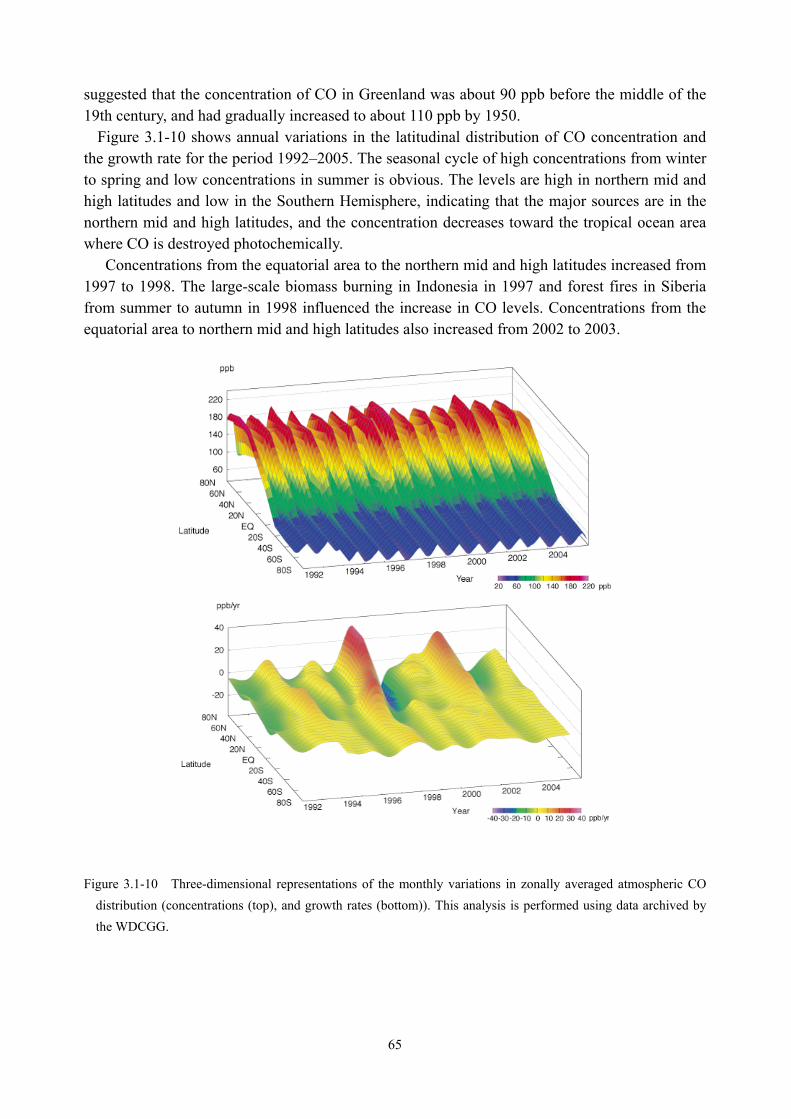
65

suggested that the concentration of CO in Greenland was about 90 ppb before the middle of the 19th century, and had gradually increased to about 110 ppb by 1950.

Figure 3.1-10 shows annual variations in the latitudinal distribution of CO concentration and the growth rate for the period 1992–2005. The seasonal cycle of high concentrations from winter to spring and low concentrations in summer is obvious. The levels are high in northern mid and high latitudes and low in the Southern Hemisphere, indicating that the major sources are in the northern mid and high latitudes, and the concentration decreases toward the tropical ocean area where CO is destroyed photochemically.

Concentrations from the equatorial area to the northern mid and high latitudes increased from 1997 to 1998. The large-scale biomass burning in Indonesia in 1997 and forest fires in Siberia from summer to autumn in 1998 influenced the increase in CO levels. Concentrations from the equatorial area to northern mid and high latitudes also increased from 2002 to 2003.

Figure 3.1-10 Three-dimensional representations of the monthly variations in zonally averaged atmospheric CO

distribution (concentrations (top), and growth rates (bottom)). This analysis is performed using data archived by the WDCGG.

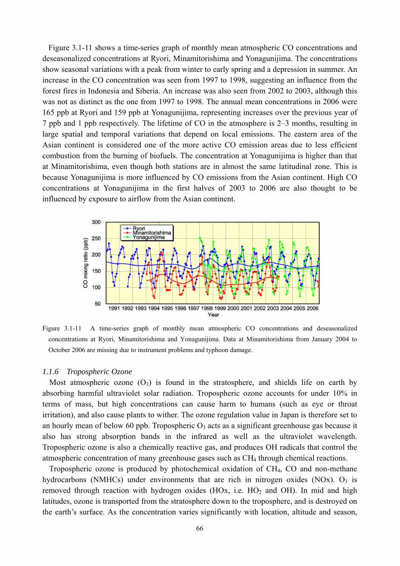
66

Figure 3.1-11 shows a time-series graph of monthly mean atmospheric CO concentrations and deseasonalized concentrations at Ryori, Minamitorishima and Yonagunijima. The concentrations show seasonal variations with a peak from winter to early spring and a depression in summer. An increase in the CO concentration was seen from 1997 to 1998, suggesting an influence from the forest fires in Indonesia and Siberia. An increase was also seen from 2002 to 2003, although this was not as distinct as the one from 1997 to 1998. The annual mean concentrations in 2006 were 165 ppb at Ryori and 159 ppb at Yonagunijima, representing increases over the previous year of 7 ppb and 1 ppb respectively. The lifetime of CO in the atmosphere is 2–3 months, resulting in large spatial and temporal variations that depend on local emissions. The eastern area of the Asian continent is considered one of the more active CO emission areas due to less efficient combustion from the burning of biofuels. The concentration at Yonagunijima is higher than that at Minamitorishima, even though both stations are in almost the same latitudinal zone. This is because Yonagunijima is more influenced by CO emissions from the Asian continent. High CO concentrations at Yonagunijima in the first halves of 2003 to 2006 are also thought to be influenced by exposure to airflow from the Asian continent.

Figure 3.1-11 A time-series graph of monthly mean atmospheric CO concentrations and deseasonalized

concentrations at Ryori, Minamitorishima and Yonagunijima. Data at Minamitorishima from January 2004 to October 2006 are missing due to instrument problems and typhoon damage.

1.1.6 Tropospheric Ozone

Most atmospheric ozone (O3) is found in the stratosphere, and shields life on earth by absorbing harmful ultraviolet solar radiation. Tropospheric ozone accounts for under 10% in terms of mass, but high concentrations can cause harm to humans (such as eye or throat irritation), and also cause plants to wither. The ozone regulation value in Japan is therefore set to an hourly mean of below 60 ppb. Tropospheric O3 acts as a significant greenhouse gas because it also has strong absorption bands in the infrared as well as the ultraviolet wavelength. Tropospheric ozone is also a chemically reactive gas, and produces OH radicals that control the atmospheric concentration of many greenhouse gases such as CH4 through chemical reactions.

Tropospheric ozone is produced by photochemical oxidation of CH4, CO and non-methane hydrocarbons (NMHCs) under environments that are rich in nitrogen oxides (NOx). O3 is removed through reaction with hydrogen oxides (HOx, i.e. HO2 and OH). In mid and high latitudes, ozone is transported from the stratosphere down to the troposphere, and is destroyed on the earth’s surface. As the concentration varies significantly with location, altitude and season,

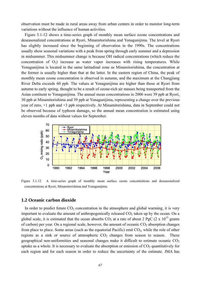
67

observation must be made in rural areas away from urban centers in order to monitor long-term variations without the influence of human activities.

Figure 3.1-12 shows a time-series graph of monthly mean surface ozone concentrations and deseasonalized concentrations at Ryori, Minamitorishima and Yonagunijima. The level at Ryori has slightly increased since the beginning of observation in the 1990s. The concentrations usually show seasonal variations with a peak from spring through early summer and a depression in midsummer. This midsummer change is because OH radical concentrations (which reduce the concentration of O3) increase as water vapor increases with rising temperatures. While Yonagunijima is located in the same latitudinal zone as Minamitorishima, the concentration at the former is usually higher than that at the latter. In the eastern region of China, the peak of monthly mean ozone concentration is observed in autumn, and the maximum at the Changjiang River Delta exceeds 60 ppb. The values at Yonagunijima are higher than those at Ryori from autumn to early spring, thought to be a result of ozone-rich air masses being transported from the Asian continent to Yonagunijima. The annual mean concentrations in 2006 were 39 ppb at Ryori, 30 ppb at Minamitorishima and 39 ppb at Yonagunijima, representing a change over the previous year of zero, +1 ppb and +3 ppb respectively. At Minamitorishima, data in September could not be observed because of typhoon damage, so the annual mean concentration is estimated using eleven months of data without values for September.

Figure 3.1-12 A time-series graph of monthly mean surface ozone concentrations and deseasonalized

concentrations at Ryori, Minamitorishima and Yonagunijima.

1.2 Oceanic carbon dioxide

In order to predict future CO2 concentration in the atmosphere and global warming, it is very important to evaluate the amount of anthropogenically released CO2 taken up by the ocean. On a global scale, it is estimated that the ocean absorbs CO2 at a rate of about 2 PgC (2 x 1015 grams of carbon) per year. On a regional scale, however, the amount of oceanic CO2 absorption changes from place to place. Some areas (such as the equatorial Pacific) emit CO2, while the role of other regions as a sink or source of atmospheric CO2 changes from season to season. These geographical non-uniformities and seasonal changes make it difficult to estimate oceanic CO2 uptake as a whole. It is necessary to evaluate the absorption or emission of CO2 quantitatively for each region and for each season in order to reduce the uncertainty of the estimate. JMA has

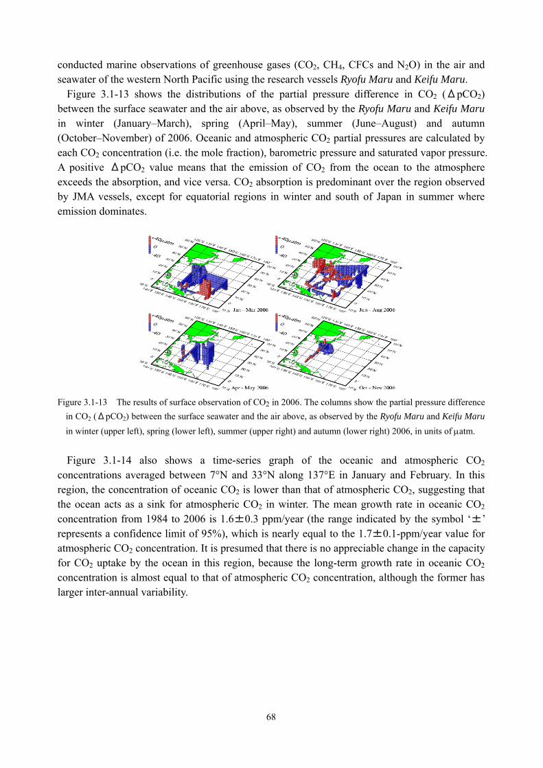
68

conducted marine observations of greenhouse gases (CO2, CH4, CFCs and N2O) in the air and seawater of the western North Pacific using the research vessels Ryofu Maru and Keifu Maru.

Figure 3.1-13 shows the distributions of the partial pressure difference in CO2 (ΔpCO2) between the surface seawater and the air above, as observed by the Ryofu Maru and Keifu Maru in winter (January–March), spring (April–May), summer (June–August) and autumn (October–November) of 2006. Oceanic and atmospheric CO2 partial pressures are calculated by each CO2 concentration (i.e. the mole fraction), barometric pressure and saturated vapor pressure. A positive ΔpCO2 value means that the emission of CO2 from the ocean to the atmosphere exceeds the absorption, and vice versa. CO2 absorption is predominant over the region observed by JMA vessels, except for equatorial regions in winter and south of Japan in summer where emission dominates.

Figure 3.1-13 The results of surface observation of CO2 in 2006. The columns show the partial pressure difference

in CO2 (ΔpCO2) between the surface seawater and the air above, as observed by the Ryofu Maru and Keifu Maru in winter (upper left), spring (lower left), summer (upper right) and autumn (lower right) 2006, in units of μatm.

Figure 3.1-14 also shows a time-series graph of the oceanic and atmospheric CO2

concentrations averaged between 7°N and 33°N along 137°E in January and February. In this region, the concentration of oceanic CO2 is lower than that of atmospheric CO2, suggesting that the ocean acts as a sink for atmospheric CO2 in winter. The mean growth rate in oceanic CO2 concentration from 1984 to 2006 is 1.6±0.3 ppm/year (the range indicated by the symbol ‘±’ represents a confidence limit of 95%), which is nearly equal to the 1.7±0.1-ppm/year value for atmospheric CO2 concentration. It is presumed that there is no appreciable change in the capacity for CO2 uptake by the ocean in this region, because the long-term growth rate in oceanic CO2 concentration is almost equal to that of atmospheric CO2 concentration, although the former has larger inter-annual variability.

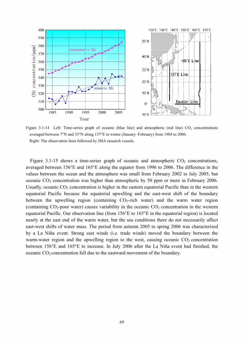
69

Figure 3.1-14 Left: Time-series graph of oceanic (blue line) and atmospheric (red line) CO2 concentrations

averaged between 7°N and 33°N along 137°E in winter (January–February) from 1984 to 2006. Right: The observation lines followed by JMA research vessels.

Figure 3.1-15 shows a time-series graph of oceanic and atmospheric CO2 concentrations, averaged between 156°E and 165°E along the equator from 1996 to 2006. The difference in the values between the ocean and the atmosphere was small from February 2002 to July 2005, but oceanic CO2 concentration was higher than atmospheric by 50 ppm or more in February 2006. Usually, oceanic CO2 concentration is higher in the eastern equatorial Pacific than in the western equatorial Pacific because the equatorial upwelling and the east-west shift of the boundary between the upwelling region (containing CO2-rich water) and the warm water region (containing CO2-poor water) causes variability in the oceanic CO2 concentration in the western equatorial Pacific. Our observation line (from 156°E to 165°E in the equatorial region) is located nearly at the east end of the warm water, but the sea conditions there do not necessarily affect east-west shifts of water mass. The period from autumn 2005 to spring 2006 was characterized by a La Niña event. Strong east winds (i.e. trade winds) moved the boundary between the warm-water region and the upwelling region to the west, causing oceanic CO2 concentration between 156°E and 165°E to increase. In July 2006 after the La Niña event had finished, the oceanic CO2 concentration fell due to the eastward movement of the boundary.

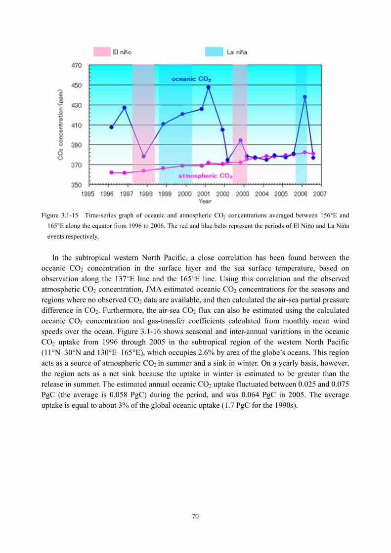
70

Figure 3.1-15 Time-series graph of oceanic and atmospheric CO2 concentrations averaged between 156°E and

165°E along the equator from 1996 to 2006. The red and blue belts represent the periods of El Niño and La Niña events respectively.

In the subtropical western North Pacific, a close correlation has been found between the

oceanic CO2 concentration in the surface layer and the sea surface temperature, based on observation along the 137°E line and the 165°E line. Using this correlation and the observed atmospheric CO2 concentration, JMA estimated oceanic CO2 concentrations for the seasons and regions where no observed CO2 data are available, and then calculated the air-sea partial pressure difference in CO2. Furthermore, the air-sea CO2 flux can also be estimated using the calculated oceanic CO2 concentration and gas-transfer coefficients calculated from monthly mean wind speeds over the ocean. Figure 3.1-16 shows seasonal and inter-annual variations in the oceanic CO2 uptake from 1996 through 2005 in the subtropical region of the western North Pacific (11°N–30°N and 130°E–165°E), which occupies 2.6% by area of the globe’s oceans. This region acts as a source of atmospheric CO2 in summer and a sink in winter. On a yearly basis, however, the region acts as a net sink because the uptake in winter is estimated to be greater than the release in summer. The estimated annual oceanic CO2 uptake fluctuated between 0.025 and 0.075 PgC (the average is 0.058 PgC) during the period, and was 0.064 PgC in 2005. The average uptake is equal to about 3% of the global oceanic uptake (1.7 PgC for the 1990s).

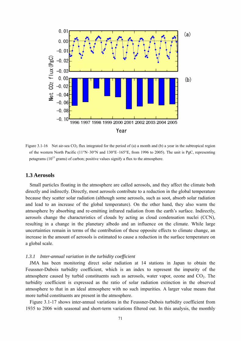
71

Figure 3.1-16 Net air-sea CO2 flux integrated for the period of (a) a month and (b) a year in the subtropical region

of the western North Pacific (11°N–30°N and 130°E–165°E, from 1996 to 2005). The unit is PgC, representing petagrams (1015 grams) of carbon; positive values signify a flux to the atmosphere.

1.3 Aerosols

Small particles floating in the atmosphere are called aerosols, and they affect the climate both directly and indirectly. Directly, most aerosols contribute to a reduction in the global temperature because they scatter solar radiation (although some aerosols, such as soot, absorb solar radiation and lead to an increase of the global temperature). On the other hand, they also warm the atmosphere by absorbing and re-emitting infrared radiation from the earth’s surface. Indirectly, aerosols change the characteristics of clouds by acting as cloud condensation nuclei (CCN), resulting in a change in the planetary albedo and an influence on the climate. While large uncertainties remain in terms of the contribution of these opposite effects to climate change, an increase in the amount of aerosols is estimated to cause a reduction in the surface temperature on a global scale.

1.3.1 Inter-annual variation in the turbidity coefficient

JMA has been monitoring direct solar radiation at 14 stations in Japan to obtain the Feussner-Dubois turbidity coefficient, which is an index to represent the impurity of the atmosphere caused by turbid constituents such as aerosols, water vapor, ozone and CO2. The turbidity coefficient is expressed as the ratio of solar radiation extinction in the observed atmosphere to that in an ideal atmosphere with no such impurities. A larger value means that more turbid constituents are present in the atmosphere.

Figure 3.1-17 shows inter-annual variations in the Feussner-Dubois turbidity coefficient from 1935 to 2006 with seasonal and short-term variations filtered out. In this analysis, the monthly

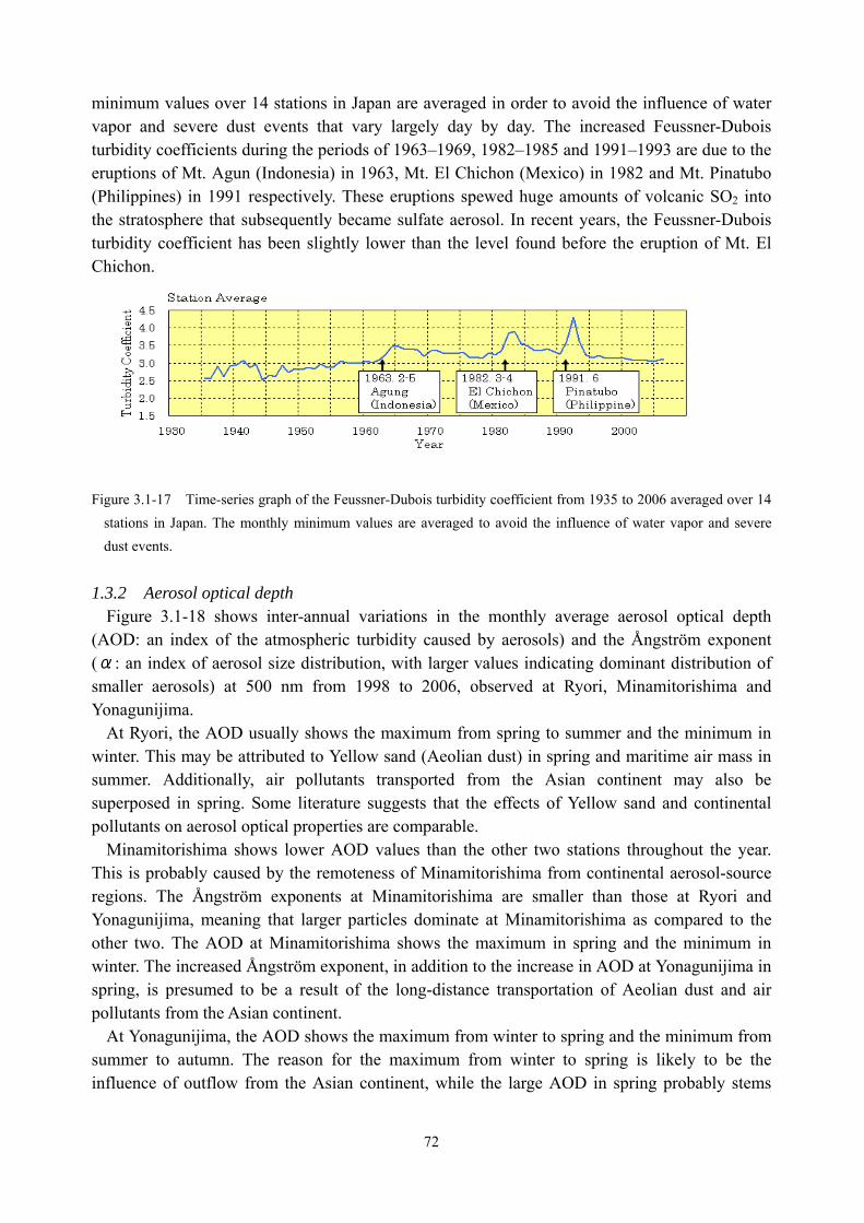
72

minimum values over 14 stations in Japan are averaged in order to avoid the influence of water vapor and severe dust events that vary largely day by day. The increased Feussner-Dubois turbidity coefficients during the periods of 1963–1969, 1982–1985 and 1991–1993 are due to the eruptions of Mt. Agun (Indonesia) in 1963, Mt. El Chichon (Mexico) in 1982 and Mt. Pinatubo (Philippines) in 1991 respectively. These eruptions spewed huge amounts of volcanic SO2 into the stratosphere that subsequently became sulfate aerosol. In recent years, the Feussner-Dubois turbidity coefficient has been slightly lower than the level found before the eruption of Mt. El Chichon.

Figure 3.1-17 Time-series graph of the Feussner-Dubois turbidity coefficient from 1935 to 2006 averaged over 14 stations in Japan. The monthly minimum values are averaged to avoid the influence of water vapor and severe dust events.

1.3.2 Aerosol optical depth Figure 3.1-18 shows inter-annual variations in the monthly average aerosol optical depth

(AOD: an index of the atmospheric turbidity caused by aerosols) and the Ångström exponent (α: an index of aerosol size distribution, with larger values indicating dominant distribution of smaller aerosols) at 500 nm from 1998 to 2006, observed at Ryori, Minamitorishima and Yonagunijima.

At Ryori, the AOD usually shows the maximum from spring to summer and the minimum in winter. This may be attributed to Yellow sand (Aeolian dust) in spring and maritime air mass in summer. Additionally, air pollutants transported from the Asian continent may also be superposed in spring. Some literature suggests that the effects of Yellow sand and continental pollutants on aerosol optical properties are comparable.

Minamitorishima shows lower AOD values than the other two stations throughout the year. This is probably caused by the remoteness of Minamitorishima from continental aerosol-source regions. The Ångström exponents at Minamitorishima are smaller than those at Ryori and Yonagunijima, meaning that larger particles dominate at Minamitorishima as compared to the other two. The AOD at Minamitorishima shows the maximum in spring and the minimum in winter. The increased Ångström exponent, in addition to the increase in AOD at Yonagunijima in spring, is presumed to be a result of the long-distance transportation of Aeolian dust and air pollutants from the Asian continent.

At Yonagunijima, the AOD shows the maximum from winter to spring and the minimum from summer to autumn. The reason for the maximum from winter to spring is likely to be the influence of outflow from the Asian continent, while the large AOD in spring probably stems

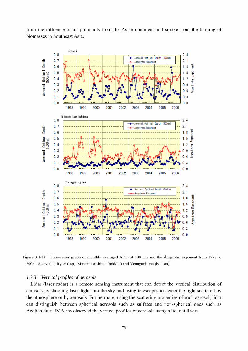
73

from the influence of air pollutants from the Asian continent and smoke from the burning of biomasses in Southeast Asia.

Figure 3.1-18 Time-series graph of monthly averaged AOD at 500 nm and the Ångström exponent from 1998 to 2006, observed at Ryori (top), Minamitorishima (middle) and Yonagunijima (bottom).

1.3.3 Vertical profiles of aerosols

Lidar (laser radar) is a remote sensing instrument that can detect the vertical distribution of aerosols by shooting laser light into the sky and using telescopes to detect the light scattered by the atmosphere or by aerosols. Furthermore, using the scattering properties of each aerosol, lidar can distinguish between spherical aerosols such as sulfates and non-spherical ones such as Aeolian dust. JMA has observed the vertical profiles of aerosols using a lidar at Ryori.

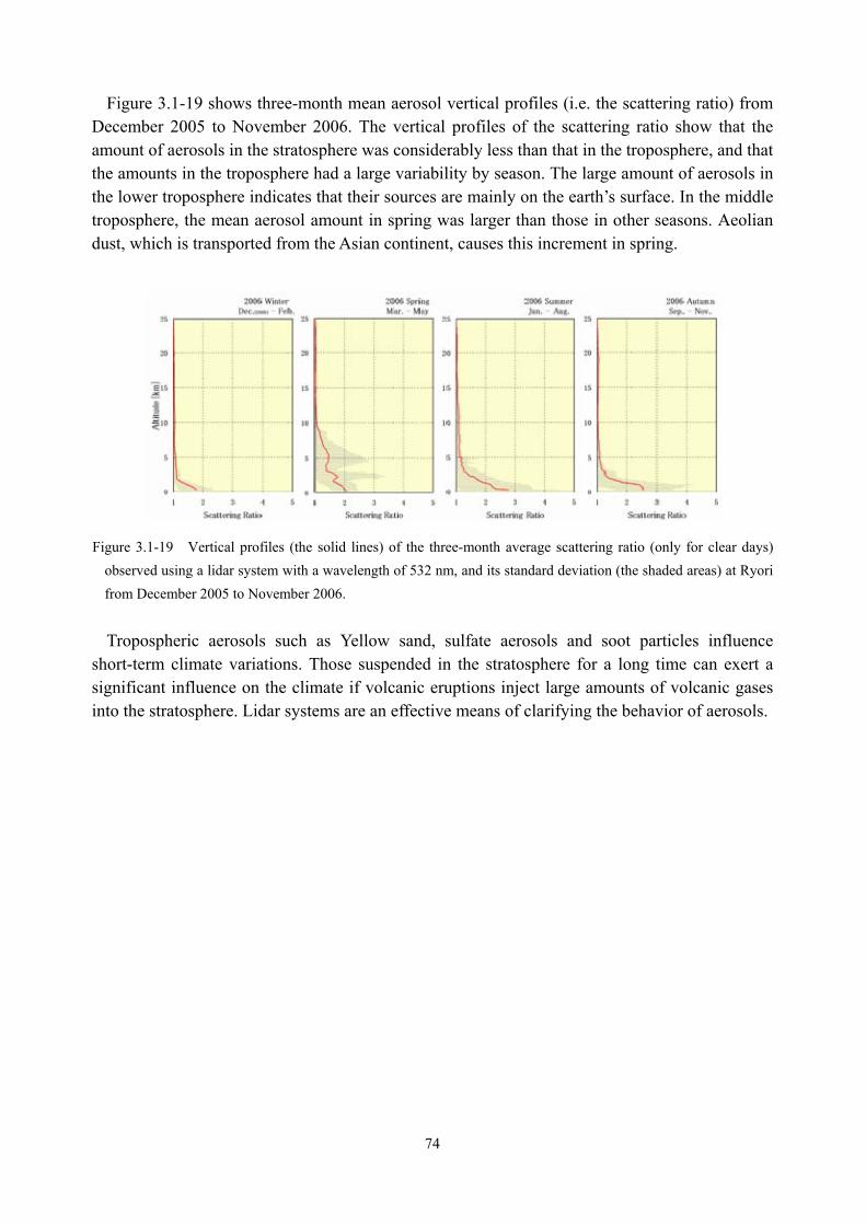
74

Figure 3.1-19 shows three-month mean aerosol vertical profiles (i.e. the scattering ratio) from December 2005 to November 2006. The vertical profiles of the scattering ratio show that the amount of aerosols in the stratosphere was considerably less than that in the troposphere, and that the amounts in the troposphere had a large variability by season. The large amount of aerosols in the lower troposphere indicates that their sources are mainly on the earth’s surface. In the middle troposphere, the mean aerosol amount in spring was larger than those in other seasons. Aeolian dust, which is transported from the Asian continent, causes this increment in spring.

Figure 3.1-19 Vertical profiles (the solid lines) of the three-month average scattering ratio (only for clear days)

observed using a lidar system with a wavelength of 532 nm, and its standard deviation (the shaded areas) at Ryori from December 2005 to November 2006.

Tropospheric aerosols such as Yellow sand, sulfate aerosols and soot particles influence

short-term climate variations. Those suspended in the stratosphere for a long time can exert a significant influence on the climate if volcanic eruptions inject large amounts of volcanic gases into the stratosphere. Lidar systems are an effective means of clarifying the behavior of aerosols.

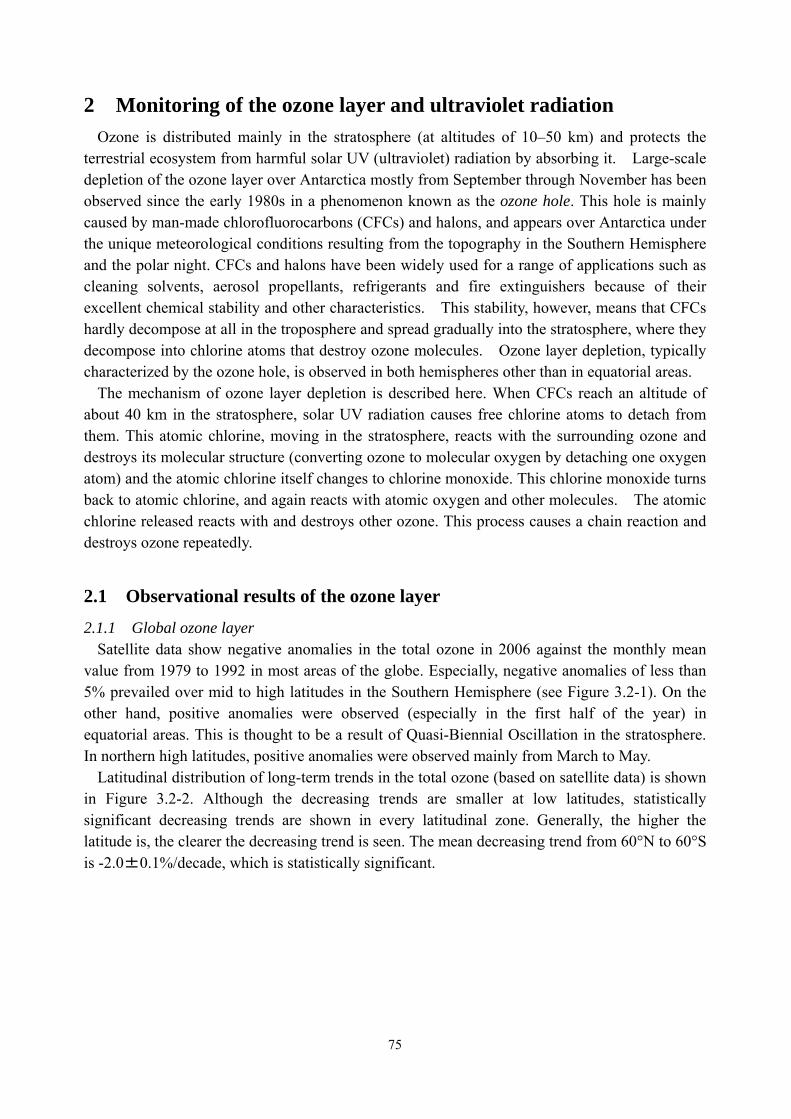
75

2 Monitoring of the ozone layer and ultraviolet radiation

Ozone is distributed mainly in the stratosphere (at altitudes of 10–50 km) and protects the terrestrial ecosystem from harmful solar UV (ultraviolet) radiation by absorbing it. Large-scale depletion of the ozone layer over Antarctica mostly from September through November has been observed since the early 1980s in a phenomenon known as the ozone hole. This hole is mainly caused by man-made chlorofluorocarbons (CFCs) and halons, and appears over Antarctica under the unique meteorological conditions resulting from the topography in the Southern Hemisphere and the polar night. CFCs and halons have been widely used for a range of applications such as cleaning solvents, aerosol propellants, refrigerants and fire extinguishers because of their excellent chemical stability and other characteristics. This stability, however, means that CFCs hardly decompose at all in the troposphere and spread gradually into the stratosphere, where they decompose into chlorine atoms that destroy ozone molecules. Ozone layer depletion, typically characterized by the ozone hole, is observed in both hemispheres other than in equatorial areas.

The mechanism of ozone layer depletion is described here. When CFCs reach an altitude of about 40 km in the stratosphere, solar UV radiation causes free chlorine atoms to detach from them. This atomic chlorine, moving in the stratosphere, reacts with the surrounding ozone and destroys its molecular structure (converting ozone to molecular oxygen by detaching one oxygen atom) and the atomic chlorine itself changes to chlorine monoxide. This chlorine monoxide turns back to atomic chlorine, and again reacts with atomic oxygen and other molecules. The atomic chlorine released reacts with and destroys other ozone. This process causes a chain reaction and destroys ozone repeatedly.

2.1 Observational results of the ozone layer

2.1.1 Global ozone layer Satellite data show negative anomalies in the total ozone in 2006 against the monthly mean

value from 1979 to 1992 in most areas of the globe. Especially, negative anomalies of less than 5% prevailed over mid to high latitudes in the Southern Hemisphere (see Figure 3.2-1). On the other hand, positive anomalies were observed (especially in the first half of the year) in equatorial areas. This is thought to be a result of Quasi-Biennial Oscillation in the stratosphere. In northern high latitudes, positive anomalies were observed mainly from March to May.

Latitudinal distribution of long-term trends in the total ozone (based on satellite data) is shown in Figure 3.2-2. Although the decreasing trends are smaller at low latitudes, statistically significant decreasing trends are shown in every latitudinal zone. Generally, the higher the latitude is, the clearer the decreasing trend is seen. The mean decreasing trend from 60°N to 60°S is -2.0±0.1%/decade, which is statistically significant.

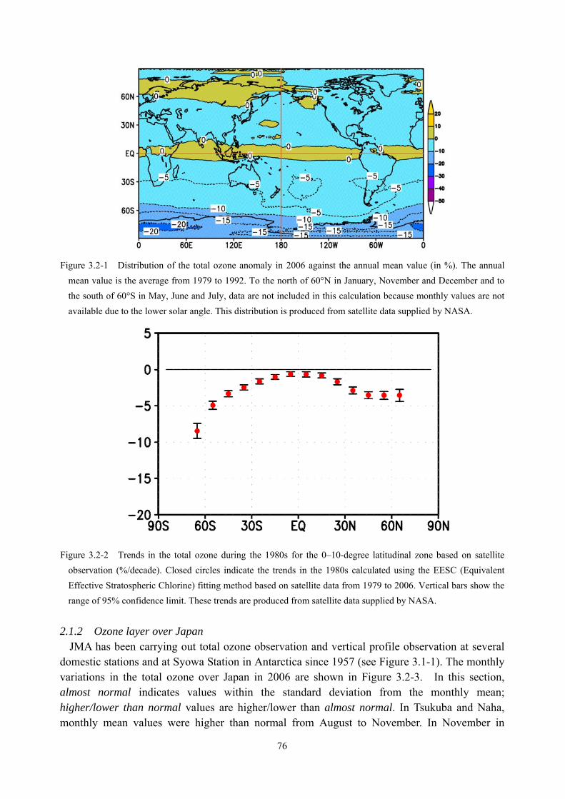
76

Figure 3.2-1 Distribution of the total ozone anomaly in 2006 against the annual mean value (in %). The annual mean value is the average from 1979 to 1992. To the north of 60°N in January, November and December and to the south of 60°S in May, June and July, data are not included in this calculation because monthly values are not available due to the lower solar angle. This distribution is produced from satellite data supplied by NASA.

Figure 3.2-2 Trends in the total ozone during the 1980s for the 0–10-degree latitudinal zone based on satellite

observation (%/decade). Closed circles indicate the trends in the 1980s calculated using the EESC (Equivalent Effective Stratospheric Chlorine) fitting method based on satellite data from 1979 to 2006. Vertical bars show the range of 95% confidence limit. These trends are produced from satellite data supplied by NASA.

2.1.2 Ozone layer over Japan

JMA has been carrying out total ozone observation and vertical profile observation at several domestic stations and at Syowa Station in Antarctica since 1957 (see Figure 3.1-1). The monthly variations in the total ozone over Japan in 2006 are shown in Figure 3.2-3. In this section, almost normal indicates values within the standard deviation from the monthly mean; higher/lower than normal values are higher/lower than almost normal. In Tsukuba and Naha, monthly mean values were higher than normal from August to November. In November in

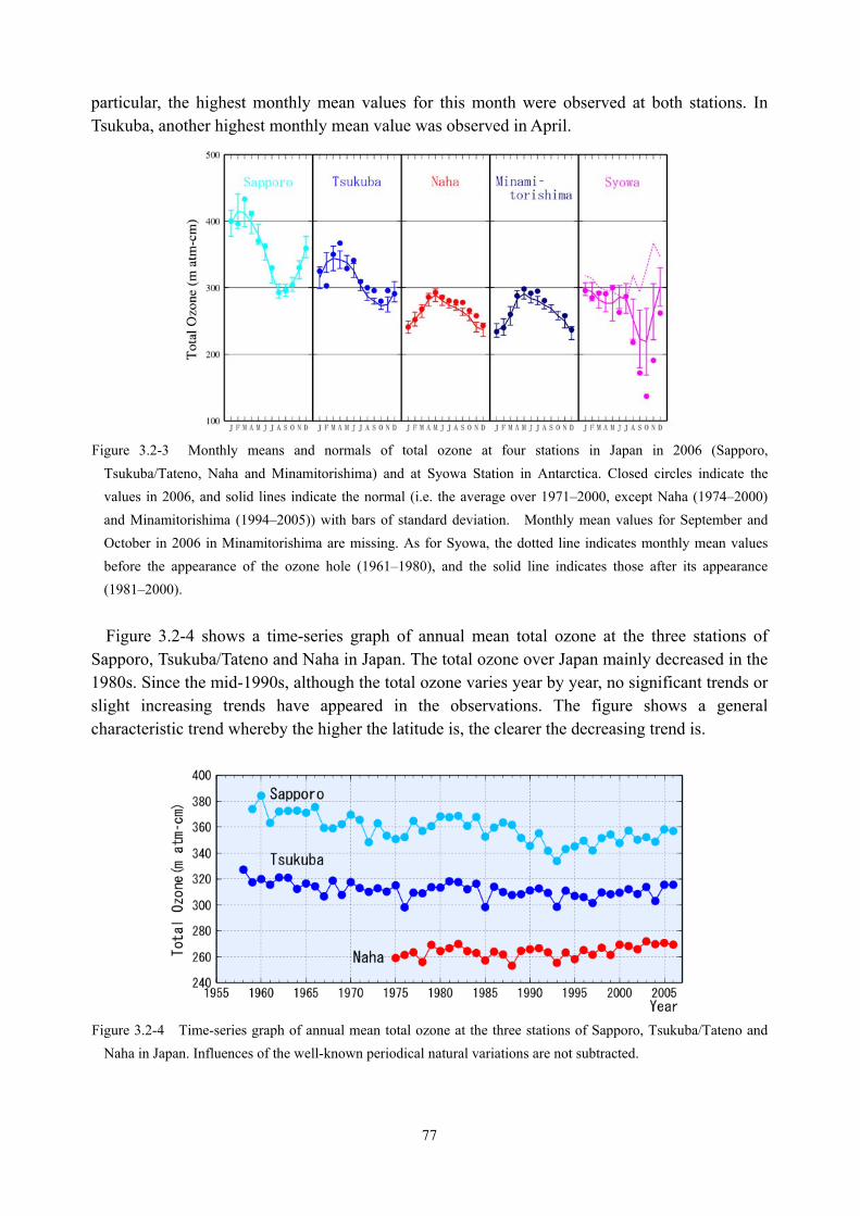
77

particular, the highest monthly mean values for this month were observed at both stations. In Tsukuba, another highest monthly mean value was observed in April.

Figure 3.2-3 Monthly means and normals of total ozone at four stations in Japan in 2006 (Sapporo,

Tsukuba/Tateno, Naha and Minamitorishima) and at Syowa Station in Antarctica. Closed circles indicate the values in 2006, and solid lines indicate the normal (i.e. the average over 1971–2000, except Naha (1974–2000) and Minamitorishima (1994–2005)) with bars of standard deviation. Monthly mean values for September and October in 2006 in Minamitorishima are missing. As for Syowa, the dotted line indicates monthly mean values before the appearance of the ozone hole (1961–1980), and the solid line indicates those after its appearance (1981–2000).

Figure 3.2-4 shows a time-series graph of annual mean total ozone at the three stations of

Sapporo, Tsukuba/Tateno and Naha in Japan. The total ozone over Japan mainly decreased in the 1980s. Since the mid-1990s, although the total ozone varies year by year, no significant trends or slight increasing trends have appeared in the observations. The figure shows a general characteristic trend whereby the higher the latitude is, the clearer the decreasing trend is.

Figure 3.2-4 Time-series graph of annual mean total ozone at the three stations of Sapporo, Tsukuba/Tateno and Naha in Japan. Influences of the well-known periodical natural variations are not subtracted.

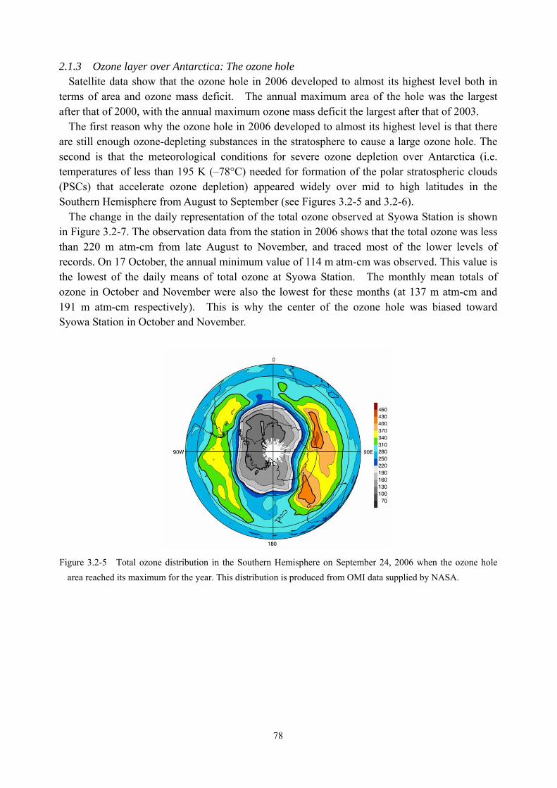
78

2.1.3 Ozone layer over Antarctica: The ozone hole Satellite data show that the ozone hole in 2006 developed to almost its highest level both in

terms of area and ozone mass deficit. The annual maximum area of the hole was the largest after that of 2000, with the annual maximum ozone mass deficit the largest after that of 2003.

The first reason why the ozone hole in 2006 developed to almost its highest level is that there are still enough ozone-depleting substances in the stratosphere to cause a large ozone hole. The second is that the meteorological conditions for severe ozone depletion over Antarctica (i.e. temperatures of less than 195 K (–78°C) needed for formation of the polar stratospheric clouds (PSCs) that accelerate ozone depletion) appeared widely over mid to high latitudes in the Southern Hemisphere from August to September (see Figures 3.2-5 and 3.2-6).

The change in the daily representation of the total ozone observed at Syowa Station is shown in Figure 3.2-7. The observation data from the station in 2006 shows that the total ozone was less than 220 m atm-cm from late August to November, and traced most of the lower levels of records. On 17 October, the annual minimum value of 114 m atm-cm was observed. This value is the lowest of the daily means of total ozone at Syowa Station. The monthly mean totals of ozone in October and November were also the lowest for these months (at 137 m atm-cm and 191 m atm-cm respectively). This is why the center of the ozone hole was biased toward Syowa Station in October and November.

Figure 3.2-5 Total ozone distribution in the Southern Hemisphere on September 24, 2006 when the ozone hole area reached its maximum for the year. This distribution is produced from OMI data supplied by NASA.

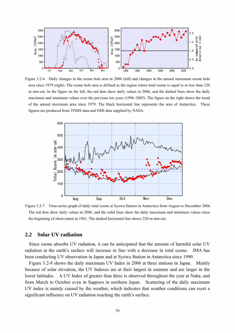
79

Figure 3.2-6 Daily changes in the ozone hole area in 2006 (left) and changes in the annual maximum ozone hole

area since 1979 (right). The ozone hole area is defined as the region where total ozone is equal to or less than 220 m atm-cm. In the figure on the left, the red dots show daily values in 2006, and the dashed lines show the daily maximum and minimum values over the previous ten years (1996–2005). The figure on the right shows the trend of the annual maximum area since 1979. The black horizontal line represents the area of Antarctica. These figures are produced from TOMS data and OMI data supplied by NASA.

Figure 3.2-7 Time-series graph of daily total ozone at Syowa Station in Antarctica from August to December 2006.

The red dots show daily values in 2006, and the solid lines show the daily maximum and minimum values since the beginning of observation in 1961. The dashed horizontal line shows 220 m atm-cm.

2.2 Solar UV radiation

Since ozone absorbs UV radiation, it can be anticipated that the amount of harmful solar UV radiation at the earth’s surface will increase in line with a decrease in total ozone. JMA has been conducting UV observation in Japan and at Syowa Station in Antarctica since 1990.

Figure 3.2-8 shows the daily maximum UV Index in 2006 at three stations in Japan. Mainly because of solar elevation, the UV Indexes are at their largest in summer and are larger in the lower latitudes. A UV Index of greater than three is observed throughout the year at Naha, and from March to October even in Sapporo in northern Japan. Scattering of the daily maximum UV index is mainly caused by the weather, which indicates that weather conditions can exert a significant influence on UV radiation reaching the earth’s surface.

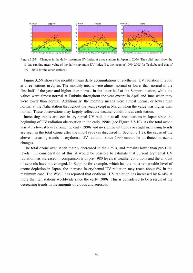
80

Figure 3.2-8 Changes in the daily maximum UV Index at three stations in Japan in 2006. The solid lines show the

15-day running mean value of the daily maximum UV Index (i.e. the mean of 1990–2005 for Tsukuba and that of 1991–2005 for the other stations).

Figure 3.2-9 shows the monthly mean daily accumulations of erythemal UV radiation in 2006

at three stations in Japan. The monthly means were almost normal or lower than normal in the first half of the year and higher than normal in the latter half at the Sapporo station, while the values were almost normal at Tsukuba throughout the year except in April and June when they were lower than normal. Additionally, the monthly means were almost normal or lower than normal at the Naha station throughout the year, except in March when the value was higher than normal. These observations may largely reflect the weather conditions at each station.

Increasing trends are seen in erythemal UV radiation at all three stations in Japan since the beginning of UV radiation observation in the early 1990s (see Figure 3.2-10). As the total ozone was at its lowest level around the early 1990s and no significant trends or slight increasing trends are seen in the total ozone after the mid-1990s (as discussed in Section 2.1.2), the cause of the above increasing trends in erythemal UV radiation since 1990 cannot be attributed to ozone changes.

The total ozone over Japan mainly decreased in the 1980s, and remains lower than pre-1980 levels. In consideration of this, it would be possible to estimate that current erythemal UV radiation has increased in comparison with pre-1980 levels if weather conditions and the amount of aerosols have not changed. In Sapporo for example, which has the most remarkable level of ozone depletion in Japan, the increase in erythemal UV radiation may reach about 6% in the maximum case. The WMO has reported that erythemal UV radiation has increased by 6-14% at more than ten stations worldwide since the early 1980s. This is considered to be a result of the decreasing trends in the amounts of clouds and aerosols.

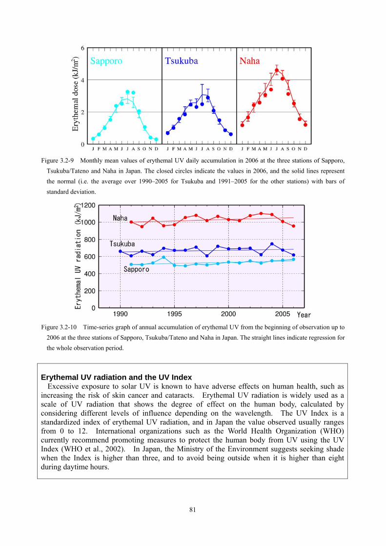
81

Figure 3.2-9 Monthly mean values of erythemal UV daily accumulation in 2006 at the three stations of Sapporo,

Tsukuba/Tateno and Naha in Japan. The closed circles indicate the values in 2006, and the solid lines represent the normal (i.e. the average over 1990–2005 for Tsukuba and 1991–2005 for the other stations) with bars of standard deviation.

Figure 3.2-10 Time-series graph of annual accumulation of erythemal UV from the beginning of observation up to

2006 at the three stations of Sapporo, Tsukuba/Tateno and Naha in Japan. The straight lines indicate regression for the whole observation period.

Erythemal UV radiation and the UV Index

Excessive exposure to solar UV is known to have adverse effects on human health, such as increasing the risk of skin cancer and cataracts. Erythemal UV radiation is widely used as a scale of UV radiation that shows the degree of effect on the human body, calculated by considering different levels of influence depending on the wavelength. The UV Index is a standardized index of erythemal UV radiation, and in Japan the value observed usually ranges from 0 to 12. International organizations such as the World Health Organization (WHO) currently recommend promoting measures to protect the human body from UV using the UV Index (WHO et al., 2002). In Japan, the Ministry of the Environment suggests seeking shade when the Index is higher than three, and to avoid being outside when it is higher than eight during daytime hours.

82

3 Yellow sand (Aeolian dust) and acid rain 3.1 Yellow sand (Aeolian dust)

Yellow sand (Aeolian dust) is a meteorological phenomenon in which fine dust in barren areas of the Asian Continent is blown up by strong winds and transported over long distances, making the atmosphere hazy. The Taklimakan Desert, the Gobi Desert and the Loess Plateau are known as places where dust particles are blown up. Such dust sometimes arrives as far as the United States or Canada across the Pacific Ocean depending on weather conditions. Research shows that the radius of most of the dust particles transported over Japan is about 1.6 micrometers, in contrast to sulfate aerosol particles that are generally smaller than 1 micrometer. Dust particles are therefore generally large in comparison with sulfate aerosols. Yellow sand is usually frequently observed in spring, although it is also sometimes seen in autumn. The latest research reveals a persistent thin dust layer over Japan during the summer.

In the source areas of yellow sand, human damage may have an impact on the occurrence of large-scale dust storms. In Japan, yellow sand causes a traffic hazard and affects laundry and vehicle bodies. It also affects the global climate through absorption and scattering of solar radiation, absorption of infrared radiation and cloud formation processes. Floating dust weakly absorbs solar radiation and heats the atmosphere, but the scattering of solar radiation simultaneously reduces the surface radiation. According to the global dust transport model developed by the Meteorological Research Institute, the presence of dust results in a weak global cooling effect of -0.3 W/m2 compared with a dust-free atmosphere. 3.1.1 Occurrences of yellow sand over Japan in 2006

JMA’s 98 meteorological stations carry out observation of yellow sand. If staff at a station observe Kosa dust, "yellow sand" is recorded.

The number of days when any meteorological station in Japan observes yellow sand (referred to below simply as the number of days) was 42 in 2006. The total daily number of meteorological stations observing yellow sand (the total daily number of stations below) was 606 in 2006. The number of days was 21 in April 2006, which is the second highest after April 2005. Yellow sand was observed extensively over Japan on April 8, 9, 18, 19, 24 and 25. In Tokyo,

the phenomenon was observed on April 18 and 19 (the first time since April 14, 2000), causing a great deal of public concern.

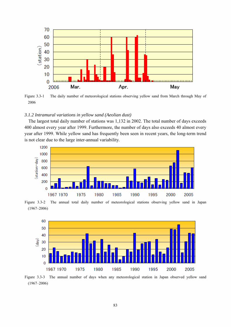
83

Figure 3.3-1 The daily number of meteorological stations observing yellow sand from March through May of

2006

3.1.2 Intramural variations in yellow sand (Aeolian dust) The largest total daily number of stations was 1,132 in 2002. The total number of days exceeds

400 almost every year after 1999. Furthermore, the number of days also exceeds 40 almost every year after 1999. While yellow sand has frequently been seen in recent years, the long-term trend is not clear due to the large inter-annual variability.

Figure 3.3-2 The annual total daily number of meteorological stations observing yellow sand in Japan

(1967–2006)

Figure 3.3-3 The annual number of days when any meteorological station in Japan observed yellow sand

(1967–2006)

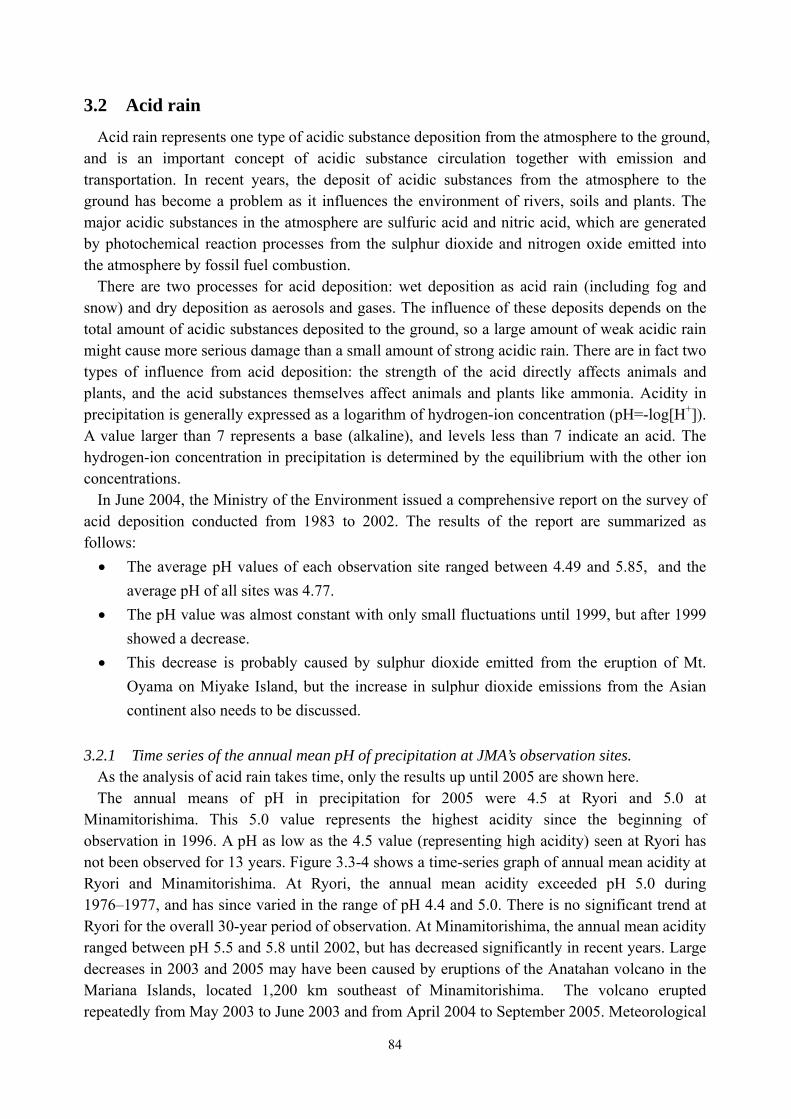
84

3.2 Acid rain

Acid rain represents one type of acidic substance deposition from the atmosphere to the ground, and is an important concept of acidic substance circulation together with emission and transportation. In recent years, the deposit of acidic substances from the atmosphere to the ground has become a problem as it influences the environment of rivers, soils and plants. The major acidic substances in the atmosphere are sulfuric acid and nitric acid, which are generated by photochemical reaction processes from the sulphur dioxide and nitrogen oxide emitted into the atmosphere by fossil fuel combustion.

There are two processes for acid deposition: wet deposition as acid rain (including fog and snow) and dry deposition as aerosols and gases. The influence of these deposits depends on the total amount of acidic substances deposited to the ground, so a large amount of weak acidic rain might cause more serious damage than a small amount of strong acidic rain. There are in fact two types of influence from acid deposition: the strength of the acid directly affects animals and plants, and the acid substances themselves affect animals and plants like ammonia. Acidity in precipitation is generally expressed as a logarithm of hydrogen-ion concentration (pH=-log[H+]). A value larger than 7 represents a base (alkaline), and levels less than 7 indicate an acid. The hydrogen-ion concentration in precipitation is determined by the equilibrium with the other ion concentrations.

In June 2004, the Ministry of the Environment issued a comprehensive report on the survey of acid deposition conducted from 1983 to 2002. The results of the report are summarized as follows: • The average pH values of each observation site ranged between 4.49 and 5.85, and the

average pH of all sites was 4.77. • The pH value was almost constant with only small fluctuations until 1999, but after 1999

showed a decrease. • This decrease is probably caused by sulphur dioxide emitted from the eruption of Mt.

Oyama on Miyake Island, but the increase in sulphur dioxide emissions from the Asian continent also needs to be discussed.

3.2.1 Time series of the annual mean pH of precipitation at JMA’s observation sites.

As the analysis of acid rain takes time, only the results up until 2005 are shown here. The annual means of pH in precipitation for 2005 were 4.5 at Ryori and 5.0 at

Minamitorishima. This 5.0 value represents the highest acidity since the beginning of observation in 1996. A pH as low as the 4.5 value (representing high acidity) seen at Ryori has not been observed for 13 years. Figure 3.3-4 shows a time-series graph of annual mean acidity at Ryori and Minamitorishima. At Ryori, the annual mean acidity exceeded pH 5.0 during 1976–1977, and has since varied in the range of pH 4.4 and 5.0. There is no significant trend at Ryori for the overall 30-year period of observation. At Minamitorishima, the annual mean acidity ranged between pH 5.5 and 5.8 until 2002, but has decreased significantly in recent years. Large decreases in 2003 and 2005 may have been caused by eruptions of the Anatahan volcano in the Mariana Islands, located 1,200 km southeast of Minamitorishima. The volcano erupted repeatedly from May 2003 to June 2003 and from April 2004 to September 2005. Meteorological

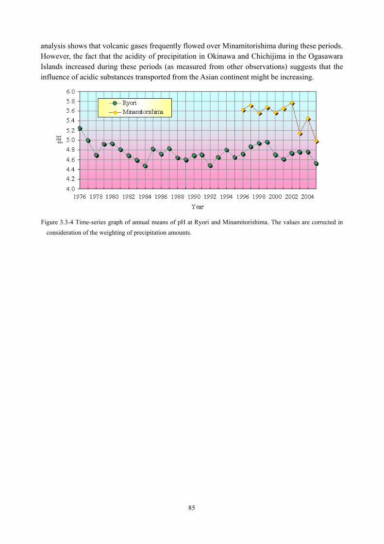
85

analysis shows that volcanic gases frequently flowed over Minamitorishima during these periods. However, the fact that the acidity of precipitation in Okinawa and Chichijima in the Ogasawara Islands increased during these periods (as measured from other observations) suggests that the influence of acidic substances transported from the Asian continent might be increasing.

Figure 3.3-4 Time-series graph of annual means of pH at Ryori and Minamitorishima. The values are corrected in consideration of the weighting of precipitation amounts.

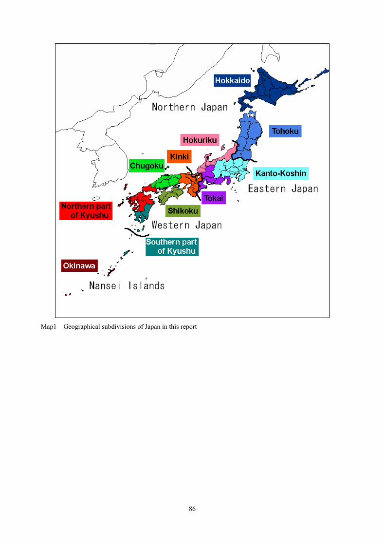
86

Map1 Geographical subdivisions of Japan in this report

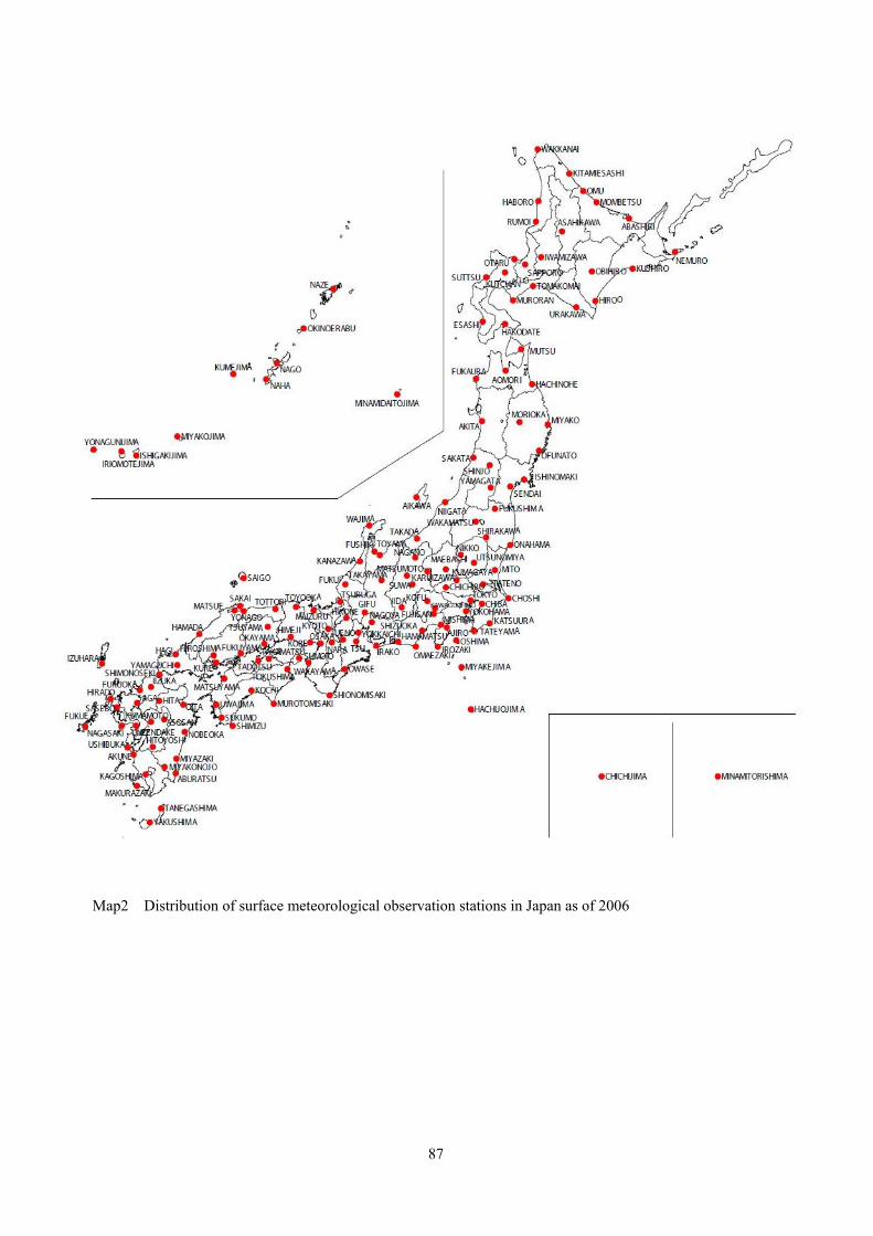
87

Map2 Distribution of surface meteorological observation stations in Japan as of 2006