Embed Size (px)
DESCRIPTION
COE 561 Digital System Design & Synthesis Logic Synthesis Background. Dr. Aiman H. El-Maleh Computer Engineering Department King Fahd University of Petroleum & Minerals. Outline. Boolean Algebra Boolean Functions Basic Definitions Representations of Boolean Functions - PowerPoint PPT Presentation
Citation preview
COE 561COE 561Digital System Design & Digital System Design &
SynthesisSynthesisLogic Synthesis BackgroundLogic Synthesis Background
COE 561COE 561Digital System Design & Digital System Design &
SynthesisSynthesisLogic Synthesis BackgroundLogic Synthesis Background
Dr. Aiman H. El-Maleh
Computer Engineering Department
King Fahd University of Petroleum & Minerals
Dr. Aiman H. El-Maleh
Computer Engineering Department
King Fahd University of Petroleum & Minerals
2
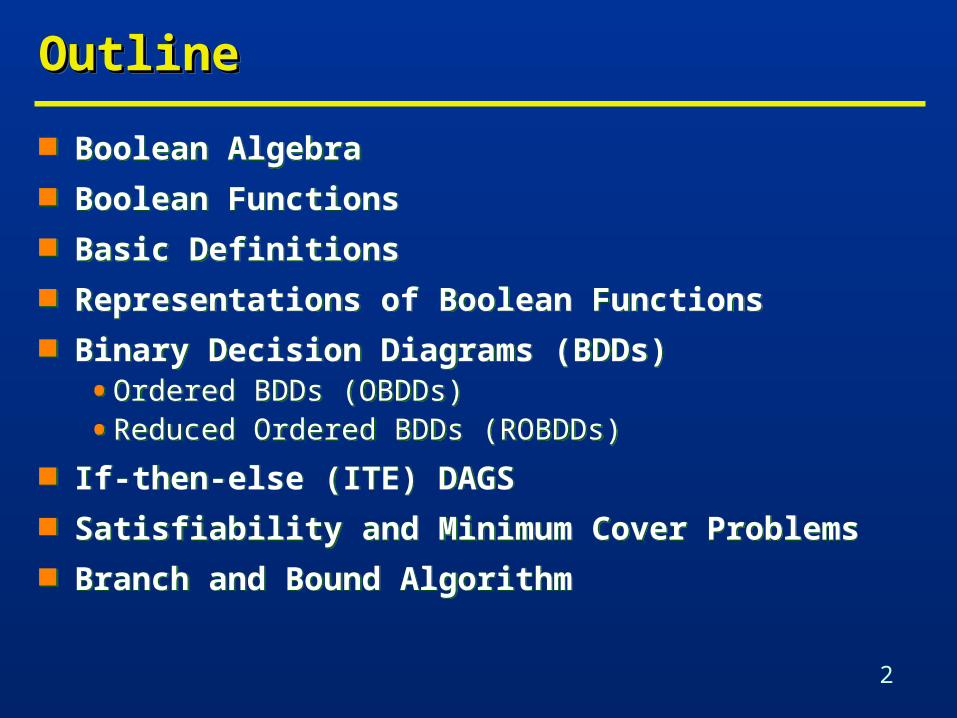
OutlineOutlineOutlineOutline
Boolean Algebra Boolean Functions Basic Definitions Representations of Boolean Functions Binary Decision Diagrams (BDDs)
• Ordered BDDs (OBDDs)
• Reduced Ordered BDDs (ROBDDs)
If-then-else (ITE) DAGS Satisfiability and Minimum Cover Problems Branch and Bound Algorithm
Boolean Algebra Boolean Functions Basic Definitions Representations of Boolean Functions Binary Decision Diagrams (BDDs)
• Ordered BDDs (OBDDs)
• Reduced Ordered BDDs (ROBDDs)
If-then-else (ITE) DAGS Satisfiability and Minimum Cover Problems Branch and Bound Algorithm
3
Boolean AlgebraBoolean AlgebraBoolean AlgebraBoolean Algebra
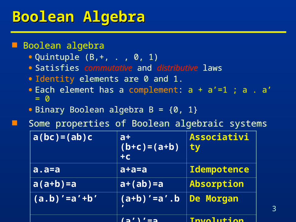
Boolean algebra• Quintuple (B,+, . , 0, 1)
• Satisfies commutative and distributive laws
• Identity elements are 0 and 1.
• Each element has a complement: a + a’=1 ; a . a’ = 0
• Binary Boolean algebra B = {0, 1}
Some properties of Boolean algebraic systems
Boolean algebra• Quintuple (B,+, . , 0, 1)
• Satisfies commutative and distributive laws
• Identity elements are 0 and 1.
• Each element has a complement: a + a’=1 ; a . a’ = 0
• Binary Boolean algebra B = {0, 1}
Some properties of Boolean algebraic systems
Associativitya+(b+c)=(a+b)+c
a(bc)=(ab)c
Idempotencea+a=aa.a=a
Absorptiona+(ab)=aa(a+b)=a
De Morgan(a+b)’=a’.b’(a.b)’=a’+b’
Involution(a’)’=a
4
Boolean FunctionsBoolean FunctionsBoolean FunctionsBoolean Functions
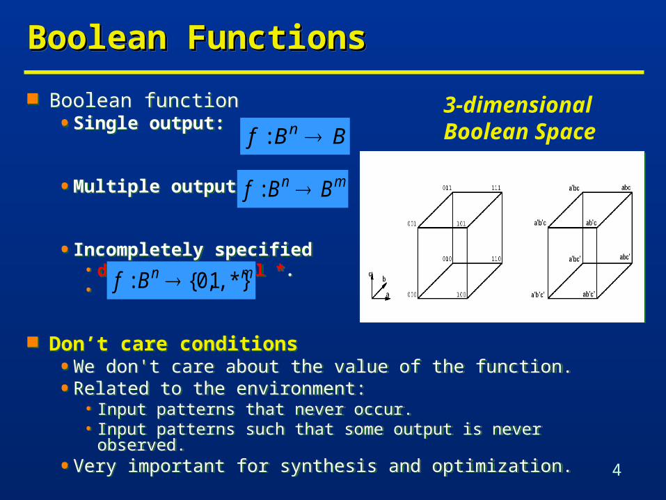
Boolean function• Single output:
• Multiple output:
• Incompletely specified• don't care symbol *.•
Don’t care conditions• We don't care about the value of the function.• Related to the environment:
• Input patterns that never occur.• Input patterns such that some output is never observed.
• Very important for synthesis and optimization.
BBf n :
mn BBf :
mnBf ,*}1,0{:
3-dimensional Boolean Space
5
Definitions …Definitions …Definitions …Definitions …
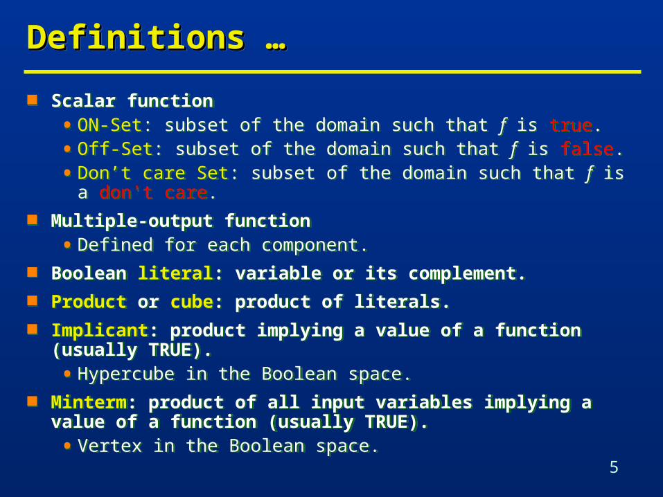
Scalar function
• ON-Set: subset of the domain such that f is true.
• Off-Set: subset of the domain such that f is false.
• Don’t care Set: subset of the domain such that f is a don't care. Multiple-output function
• Defined for each component. Boolean literal: variable or its complement. Product or cube: product of literals. Implicant: product implying a value of a function (usually TRUE).
• Hypercube in the Boolean space. Minterm: product of all input variables implying a value of a
function (usually TRUE).
• Vertex in the Boolean space.
6
… … Definitions …Definitions …… … Definitions …Definitions …
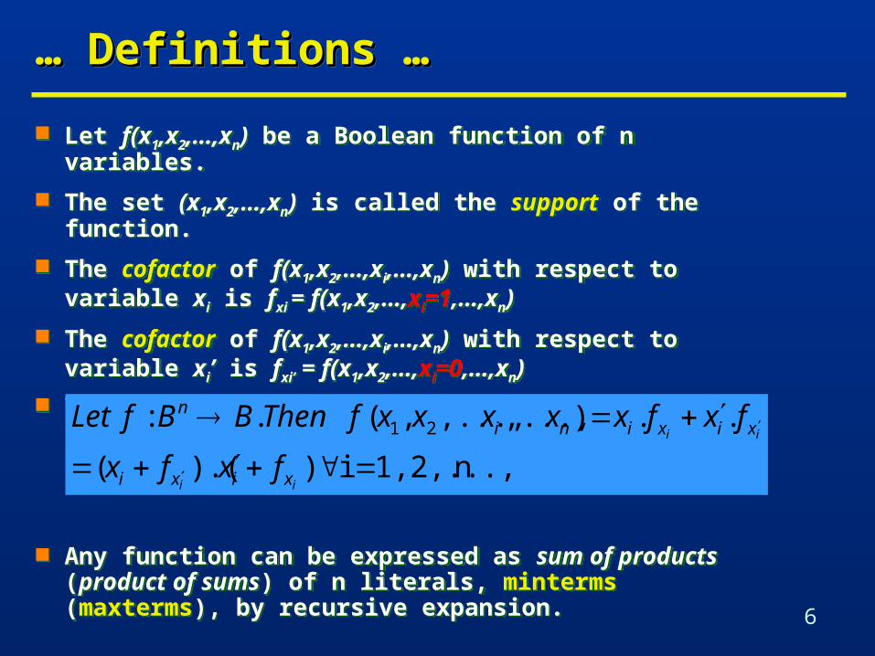
Let f(x1,x2,…,xn) be a Boolean function of n variables.
The set (x1,x2,…,xn) is called the support of the function.
The cofactor of f(x1,x2,…,xi,…,xn) with respect to variable xi is fxi = f(x1,x2,…,xi=1,…,xn)
The cofactor of f(x1,x2,…,xi,…,xn) with respect to variable xi’ is fxi’ = f(x1,x2,…,xi=0,…,xn)
Theorem: Shannon's Expansion
Any function can be expressed as sum of products (product of sums) of n literals, minterms (maxterms), by recursive expansion.
n1,2,...,i )).((
..),...,,...,,( .: 21
ii
ii
xixi
xixinin
fxfx
fxfxxxxxfThenBBfLet
7
… … Definitions …Definitions …… … Definitions …Definitions …
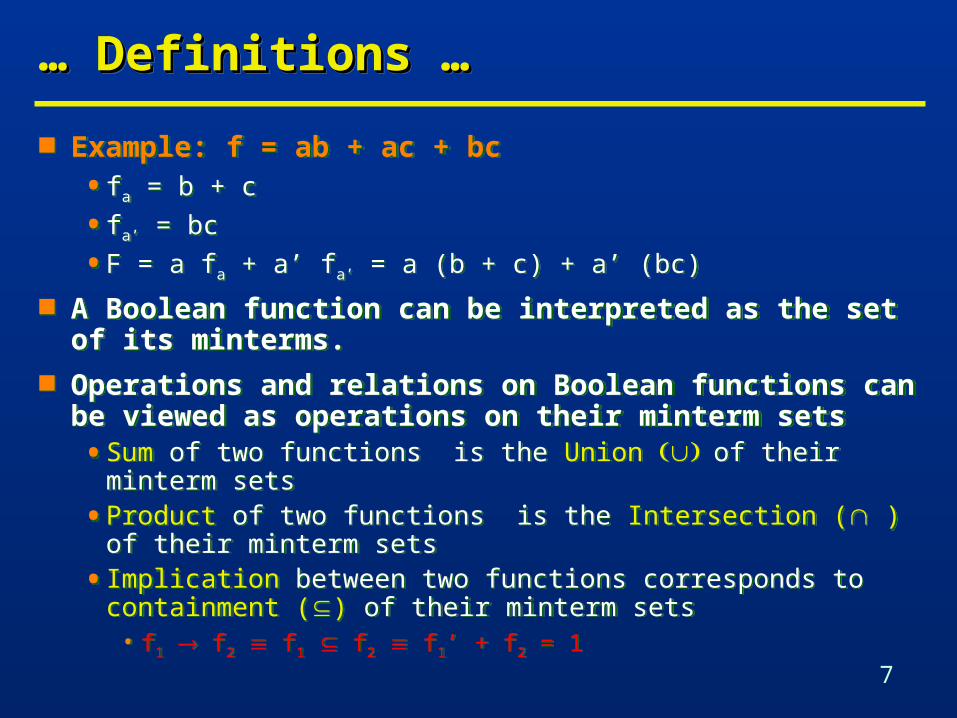
Example: f = ab + ac + bc
• fa = b + c
• fa’ = bc
• F = a fa + a’ fa’ = a (b + c) + a’ (bc)
A Boolean function can be interpreted as the set of its minterms.
Operations and relations on Boolean functions can be viewed as operations on their minterm sets• Sum of two functions is the Union of their minterm sets
• Product of two functions is the Intersection ( ) of their minterm sets
• Implication between two functions corresponds to containment () of their minterm sets
• f1 f2 f1 f2 f1’ + f2 = 1
8
… … Definitions …Definitions …… … Definitions …Definitions …
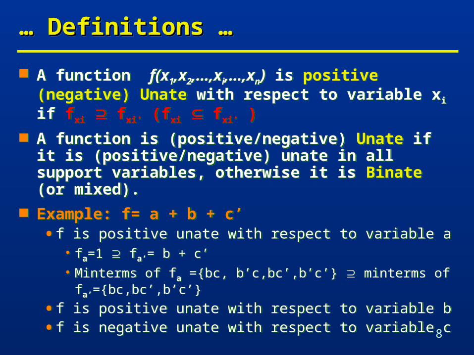
A function f(x1,x2,…,xi,…,xn) is positive (negative) Unate with respect to variable xi if fxi fxi’ (fxi fxi’ )
A function is (positive/negative) Unate if it is (positive/negative) unate in all support variables, otherwise it is Binate (or mixed).
Example: f= a + b + c’• f is positive unate with respect to variable a
• fa=1 fa’= b + c’
• Minterms of fa ={bc, b’c,bc’,b’c’} minterms of fa’={bc,bc’,b’c’}
• f is positive unate with respect to variable b
• f is negative unate with respect to variable c
9
… … DefinitionsDefinitions… … DefinitionsDefinitions
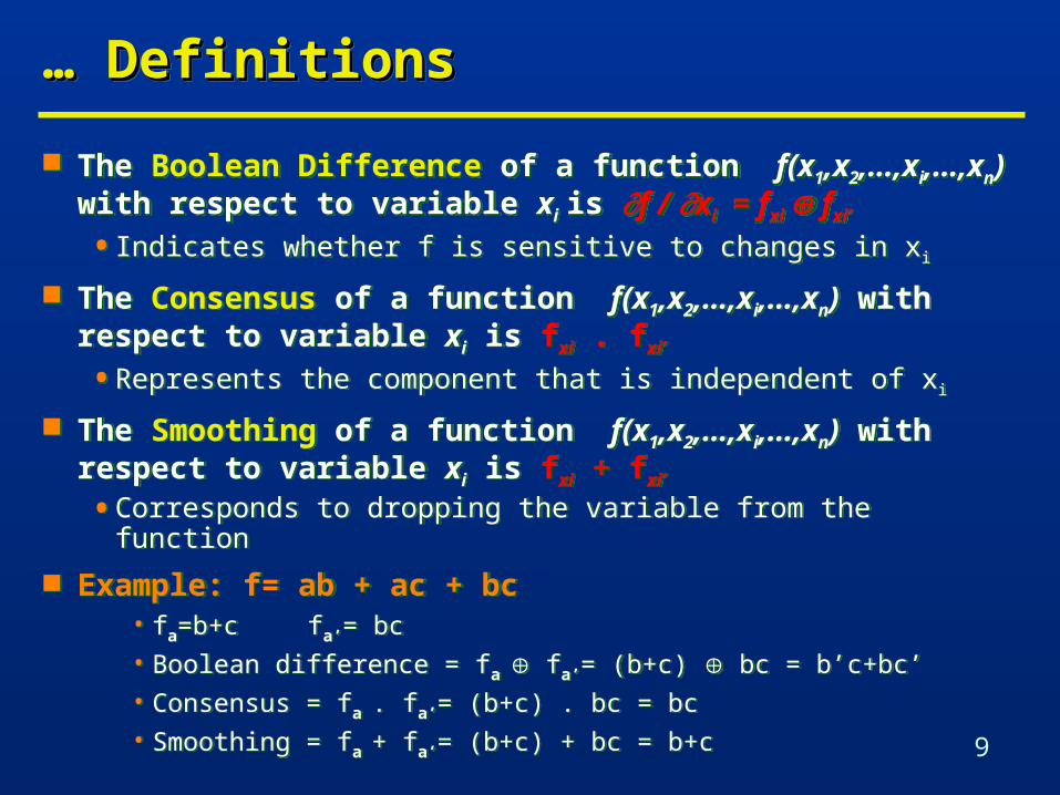
The Boolean Difference of a function f(x1,x2,…,xi,…,xn) with respect to variable xi is f / xi = fxi fxi’
• Indicates whether f is sensitive to changes in xi
The Consensus of a function f(x1,x2,…,xi,…,xn) with respect to variable xi is fxi . fxi’
• Represents the component that is independent of xi
The Smoothing of a function f(x1,x2,…,xi,…,xn) with respect to variable xi is fxi + fxi’
• Corresponds to dropping the variable from the function
Example: f= ab + ac + bc• fa=b+c fa’= bc
• Boolean difference = fa fa’= (b+c) bc = b’c+bc’
• Consensus = fa . fa’= (b+c) . bc = bc
• Smoothing = fa + fa’= (b+c) + bc = b+c

10
Boolean Expansion Based on Orthonormal Boolean Expansion Based on Orthonormal Basis …Basis …Boolean Expansion Based on Orthonormal Boolean Expansion Based on Orthonormal Basis …Basis …
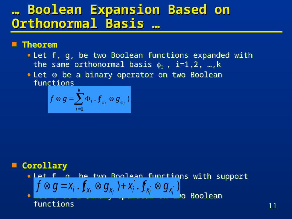
Let i , i=1,2, …,k be a set of Boolean functions such that i=1 to k i = 1 and i . j = 0 for i j {1,2,…,k}.
An Orthonormal Expansion of a function f is
f= i=1 to k fi . i
fi is called the generalized cofactor of f w.r.t. i i.
The generalized cofactor may not be unique
• f . i fi f + i ‘
Example: f = ab+ac+bc; 1 = ab; 2 = a’+b’;
• ab f1 1 ; let f1 = 1
• a’bc+ab’c f2 ab+bc+ac ; let f2 = a’bc+ab’c
• f = I fI . + 2 f2 = ab (1) + (a’+b’)(a’bc+ab’c)=ab+bc+ac
11
… … Boolean Expansion Based on Boolean Expansion Based on Orthonormal Basis …Orthonormal Basis …… … Boolean Expansion Based on Boolean Expansion Based on Orthonormal Basis …Orthonormal Basis …
Theorem• Let f, g, be two Boolean functions expanded with the same
orthonormal basis I , i=1,2, …,k
• Let be a binary operator on two Boolean functions
Corollary
• Let f, g, be two Boolean functions with support variables {xi, i=1,2, …,n}.
• Let be a binary operator on two Boolean functions
Theorem• Let f, g, be two Boolean functions expanded with the same
orthonormal basis I , i=1,2, …,k
• Let be a binary operator on two Boolean functions
Corollary
• Let f, g, be two Boolean functions with support variables {xi, i=1,2, …,n}.
• Let be a binary operator on two Boolean functions
).(1
iigfgf
k
i
i
).().(iiii xxixxi gfxgfxgf
12
… … Boolean Expansion Based on Boolean Expansion Based on Orthonormal BasisOrthonormal Basis… … Boolean Expansion Based on Boolean Expansion Based on Orthonormal BasisOrthonormal Basis
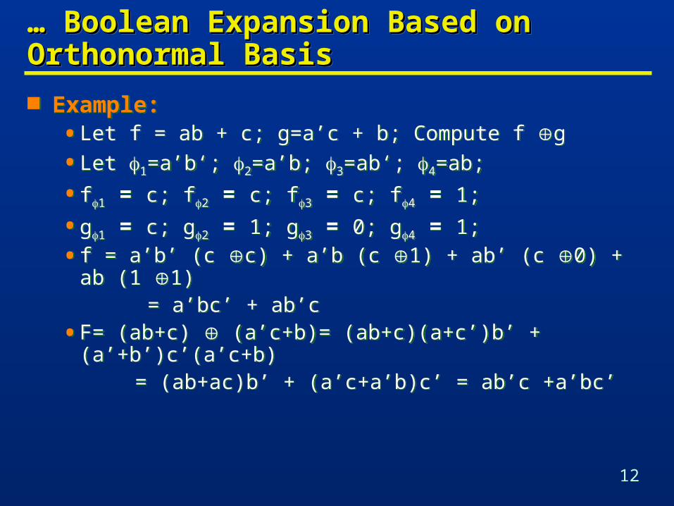
Example:• Let f = ab + c; g=a’c + b; Compute f g
• Let 1=a’b‘; 2=a’b; 3=ab‘; 4=ab;
• f1 = c; f2 = c; f3 = c; f4 = 1;
• g1 = c; g2 = 1; g3 = 0; g4 = 1;
• f = a’b’ (c c) + a’b (c 1) + ab’ (c 0) + ab (1 1) = a’bc’ + ab’c
• F= (ab+c) (a’c+b)= (ab+c)(a+c’)b’ + (a’+b’)c’(a’c+b) = (ab+ac)b’ + (a’c+a’b)c’ = ab’c +a’bc’
13
Representations of Boolean FunctionsRepresentations of Boolean FunctionsRepresentations of Boolean FunctionsRepresentations of Boolean Functions
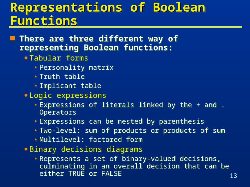
There are three different way of representing Boolean functions:• Tabular forms
• Personality matrix• Truth table• Implicant table
• Logic expressions• Expressions of literals linked by the + and . Operators• Expressions can be nested by parenthesis• Two-level: sum of products or products of sum• Multilevel: factored form
• Binary decisions diagrams• Represents a set of binary-valued decisions, culminating in an
overall decision that can be either TRUE or FALSE
14
Tabular RepresentationsTabular RepresentationsTabular RepresentationsTabular Representations
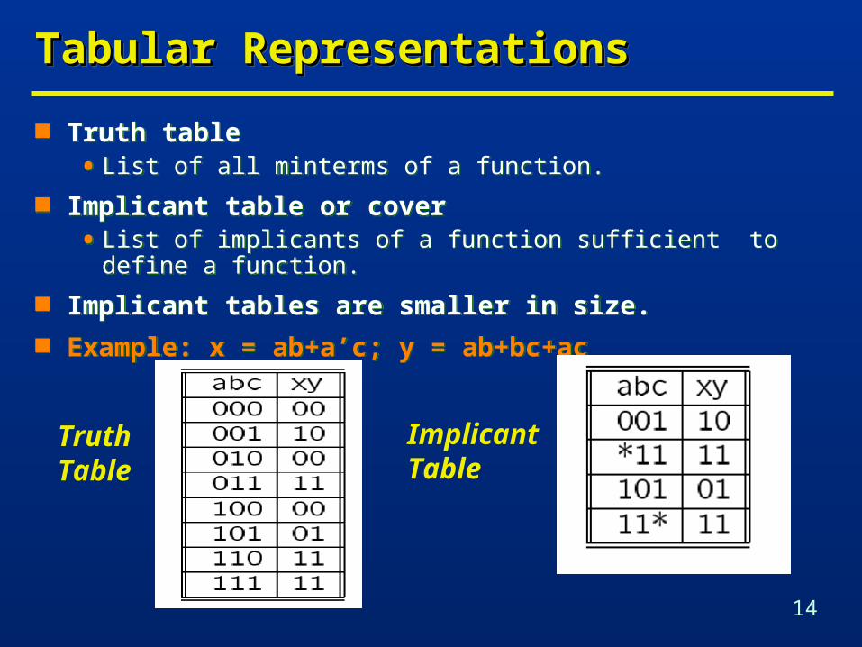
Truth table• List of all minterms of a function.
Implicant table or cover• List of implicants of a function sufficient to define a function.
Implicant tables are smaller in size. Example: x = ab+a’c; y = ab+bc+ac
Truth table• List of all minterms of a function.
Implicant table or cover• List of implicants of a function sufficient to define a function.
Implicant tables are smaller in size. Example: x = ab+a’c; y = ab+bc+ac
Truth Table
Implicant Table
15
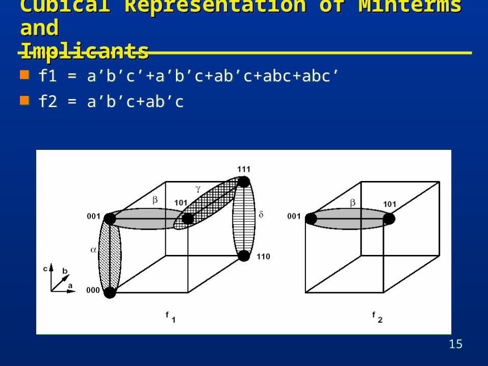
Cubical Representation of Minterms andCubical Representation of Minterms andImplicantsImplicantsCubical Representation of Minterms andCubical Representation of Minterms andImplicantsImplicants
f1 = a’b’c’+a’b’c+ab’c+abc+abc’ f2 = a’b’c+ab’c
f1 = a’b’c’+a’b’c+ab’c+abc+abc’ f2 = a’b’c+ab’c
16
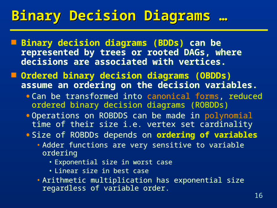
Binary Decision Diagrams …Binary Decision Diagrams …Binary Decision Diagrams …Binary Decision Diagrams …
Binary decision diagrams (BDDs) can be represented by trees or rooted DAGs, where decisions are associated with vertices.
Ordered binary decision diagrams (OBDDs) assume an ordering on the decision variables.• Can be transformed into canonical forms, reduced ordered
binary decision diagrams (ROBDDs)
• Operations on ROBDDS can be made in polynomial time of their size i.e. vertex set cardinality
• Size of ROBDDs depends on ordering of variables• Adder functions are very sensitive to variable ordering
• Exponential size in worst case• Linear size in best case
• Arithmetic multiplication has exponential size regardless of variable order.
17
… … Binary Decision Diagrams …Binary Decision Diagrams …… … Binary Decision Diagrams …Binary Decision Diagrams …
An OBDD is a rooted DAG with vertex set V. Each non-leaf vertex has as attributes
• a pointer index(v) {1,2,…n} to an input variable {x1,x2,…,xi,…,xn} .
• Two children low(v) and high(v) V.
A leaf vertex v has as an attribute a value value(v) B. For any vertex pair {v,low(v)} (and {v,high(v)}) such that
no vertex is a leaf, index(v)<index(low(v)) (index(v)<index(high(v))
An OBDD with root v denotes a function fv such that• If v is a leaf with value(v)=1, then fv=1
• If v is a leaf with value(v)=0, then fv=0
• If v is not a leaf and index(v)=i, then fv= xi ‘ . flow(v) + xi . fhigh(v)
18
… … Binary Decision DiagramsBinary Decision Diagrams… … Binary Decision DiagramsBinary Decision Diagrams
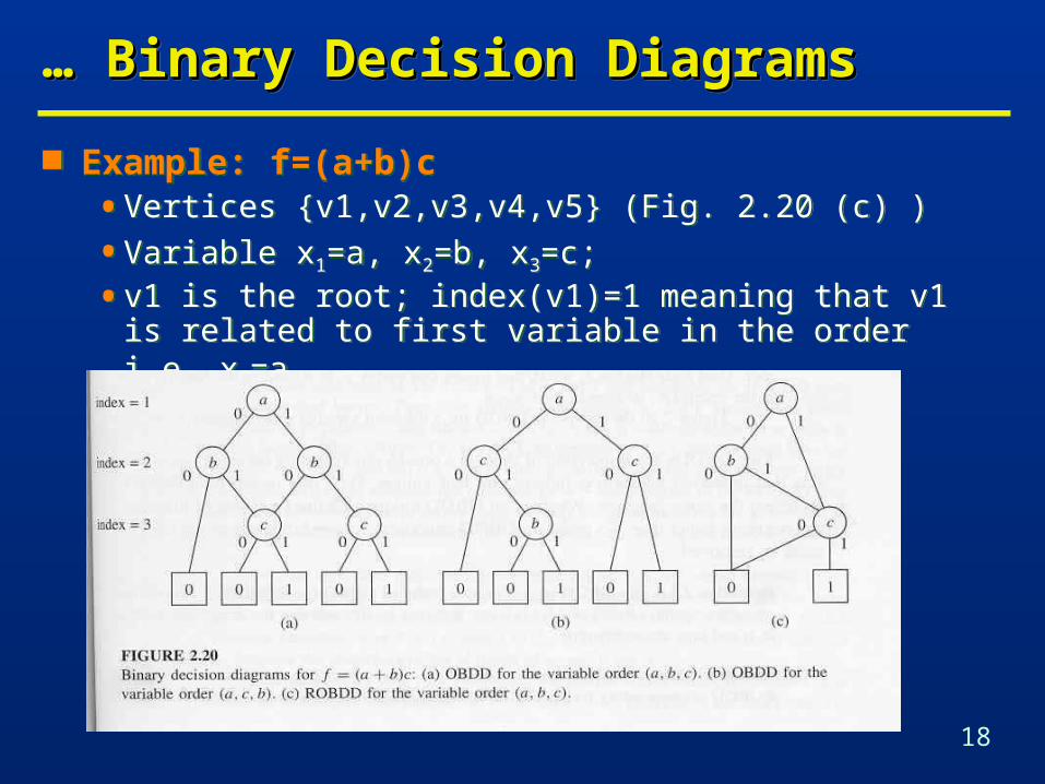
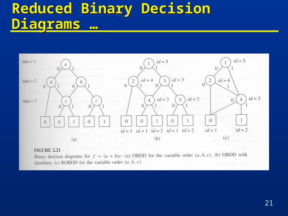
Example: f=(a+b)c• Vertices {v1,v2,v3,v4,v5} (Fig. 2.20 (c) )
• Variable x1=a, x2=b, x3=c;
• v1 is the root; index(v1)=1 meaning that v1 is related to first variable in the order i.e. x1=a
Example: f=(a+b)c• Vertices {v1,v2,v3,v4,v5} (Fig. 2.20 (c) )
• Variable x1=a, x2=b, x3=c;
• v1 is the root; index(v1)=1 meaning that v1 is related to first variable in the order i.e. x1=a
19
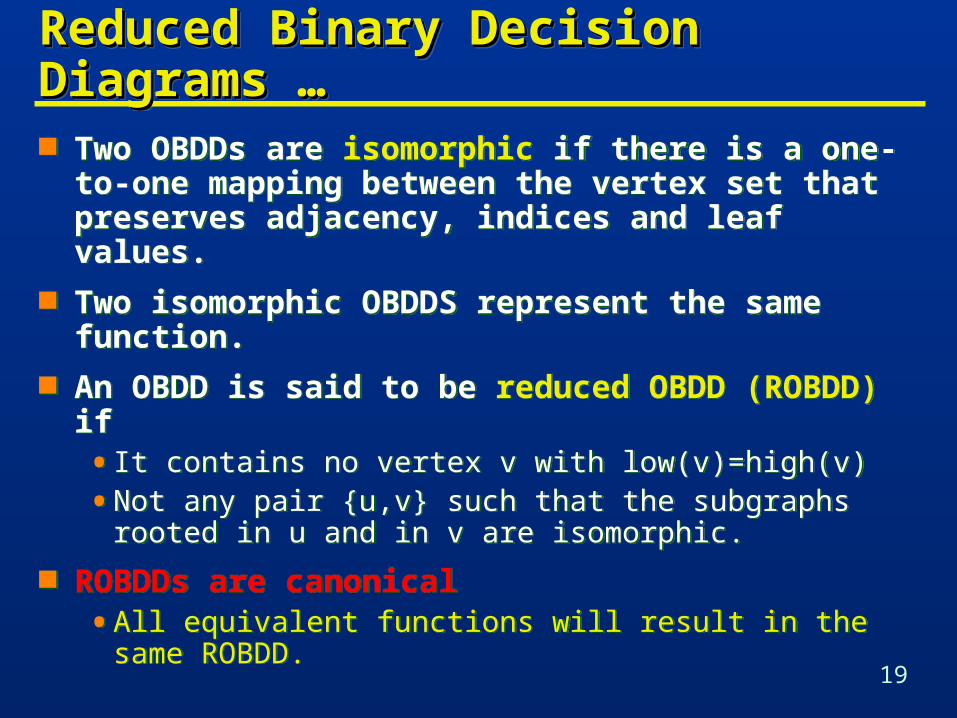
Reduced Binary Decision Diagrams …Reduced Binary Decision Diagrams …Reduced Binary Decision Diagrams …Reduced Binary Decision Diagrams …
Two OBDDs are isomorphic if there is a one-to-one mapping between the vertex set that preserves adjacency, indices and leaf values.
Two isomorphic OBDDS represent the same function. An OBDD is said to be reduced OBDD (ROBDD) if
• It contains no vertex v with low(v)=high(v)
• Not any pair {u,v} such that the subgraphs rooted in u and in v are isomorphic.
ROBDDs are canonical• All equivalent functions will result in the same ROBDD.
20
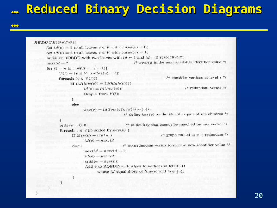
… … Reduced Binary Decision Diagrams …Reduced Binary Decision Diagrams …… … Reduced Binary Decision Diagrams …Reduced Binary Decision Diagrams …
21
Reduced Binary Decision Diagrams …Reduced Binary Decision Diagrams …Reduced Binary Decision Diagrams …Reduced Binary Decision Diagrams …
22
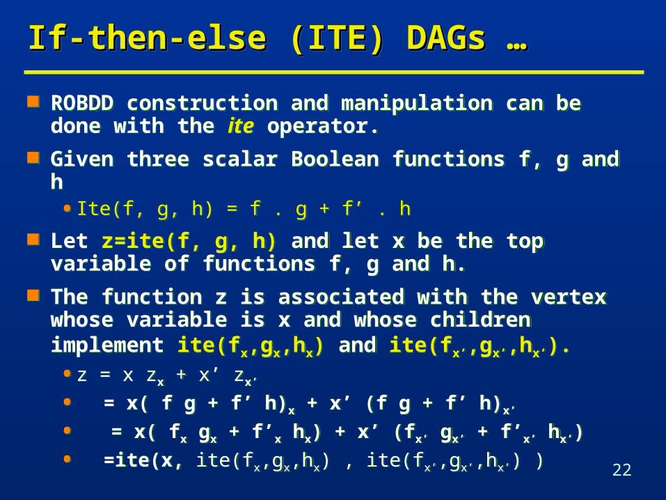
If-then-else (ITE) DAGs …If-then-else (ITE) DAGs …If-then-else (ITE) DAGs …If-then-else (ITE) DAGs …
ROBDD construction and manipulation can be done with the ite operator.
Given three scalar Boolean functions f, g and h• Ite(f, g, h) = f . g + f’ . h
Let z=ite(f, g, h) and let x be the top variable of functions f, g and h.
The function z is associated with the vertex whose variable is x and whose children implement ite(fx,gx,hx) and ite(fx’,gx’,hx’).
• z = x zx + x’ zx’
• = x( f g + f’ h)x + x’ (f g + f’ h)x’
• = x( fx gx + f’x hx) + x’ (fx’ gx’ + f’x’ hx’)
• =ite(x, ite(fx,gx,hx) , ite(fx’,gx’,hx’) )
23
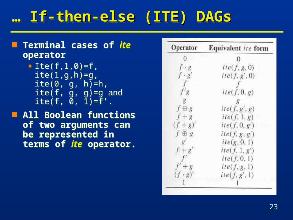
… … If-then-else (ITE) DAGsIf-then-else (ITE) DAGs… … If-then-else (ITE) DAGsIf-then-else (ITE) DAGs
Terminal cases of ite operator• Ite(f,1,0)=f, ite(1,g,h)=g,
ite(0, g, h)=h, ite(f, g, g)=g and ite(f, 0, 1)=f’.
All Boolean functions of two arguments can be represented in terms of ite operator.
Terminal cases of ite operator• Ite(f,1,0)=f, ite(1,g,h)=g,
ite(0, g, h)=h, ite(f, g, g)=g and ite(f, 0, 1)=f’.
All Boolean functions of two arguments can be represented in terms of ite operator.
24
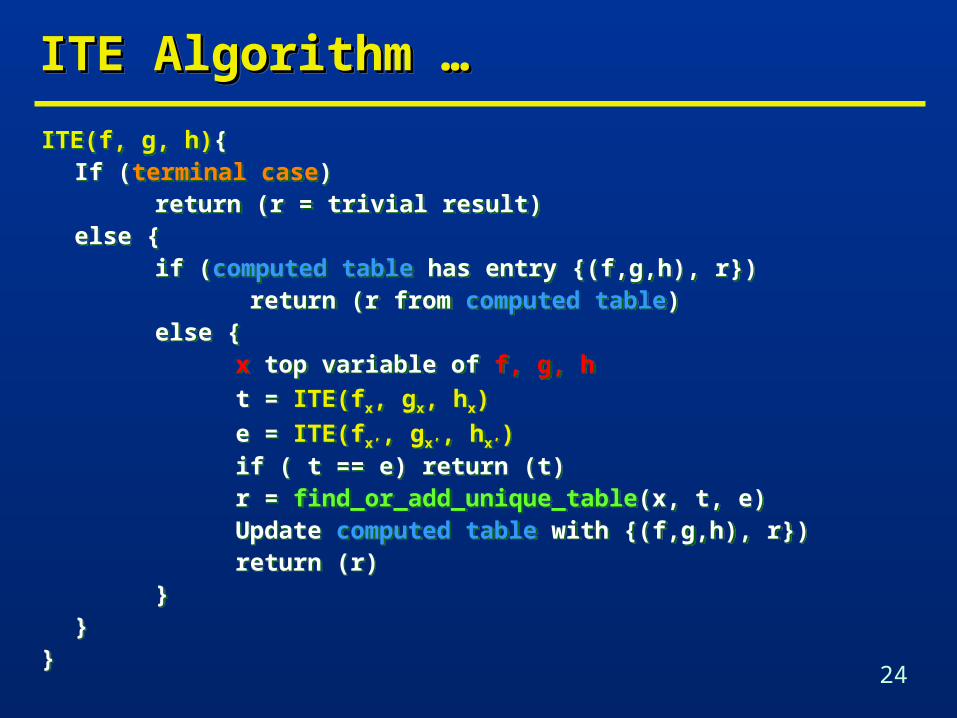
ITE Algorithm …ITE Algorithm …ITE Algorithm …ITE Algorithm …
ITE(f, g, h){If (terminal case)
return (r = trivial result)else {
if (computed table has entry {(f,g,h), r}) return (r from computed table)
else {x top variable of f, g, h
t = ITE(fx, gx, hx)
e = ITE(fx’, gx’, hx’) if ( t == e) return (t)r = find_or_add_unique_table(x, t, e)Update computed table with {(f,g,h), r})return (r)
}}
}
25
… … ITE AlgorithmITE Algorithm… … ITE AlgorithmITE Algorithm
Uses two tables• Unique table: stores ROBDD information in a strong
canonical form• Equivalence check is just a test on the equality of the identifiers• Contains a key for a vertex of an ROBDD• Key is a triple of variable, identifiers of left and right children
• Computed table: to improve the performance of the algorithm• Mapping between any tripe (f, g, h) and vertex implementing
ite(f, g, h).
26
Applications of ITE DAGsApplications of ITE DAGsApplications of ITE DAGsApplications of ITE DAGs
Implication of two functions is Tautology• f g f’ + g = 1
• Check if ite(f, g, 1) has identifier equal to that of leaf value 1
• Alternatively, a function associated with a vertex is tautology if both of its children are tautology
Functional composition • Replacing a variable by another expression
• fx=g = fx g + fx’ g’ = ite(g, fx, fx’)
Consensus
• fx . fx’ ite(fx, fx’, 0)
Smoothing
• fx + fx’ ite(fx,1, fx’)
27
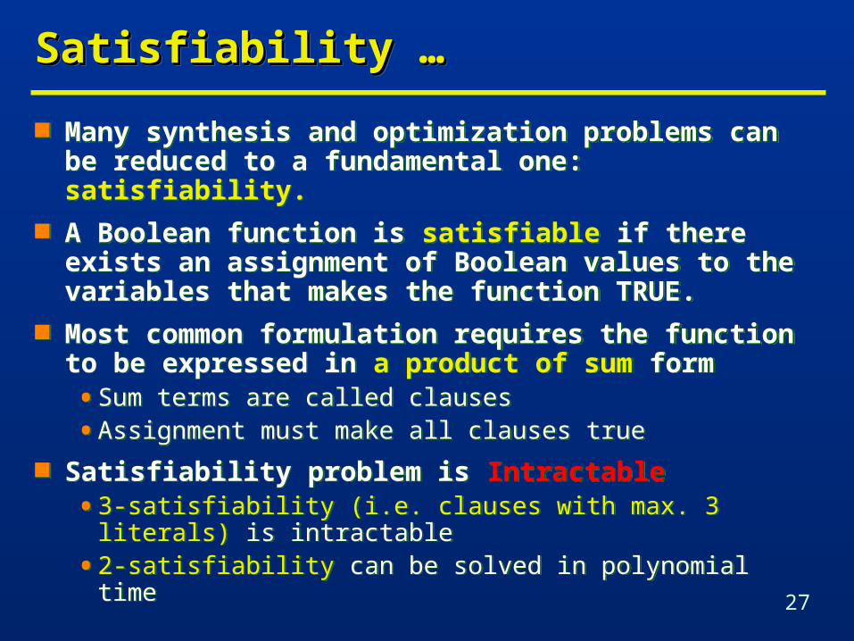
Satisfiability …Satisfiability …Satisfiability …Satisfiability …
Many synthesis and optimization problems can be reduced to a fundamental one: satisfiability.
A Boolean function is satisfiable if there exists an assignment of Boolean values to the variables that makes the function TRUE.
Most common formulation requires the function to be expressed in a product of sum form • Sum terms are called clauses
• Assignment must make all clauses true
Satisfiability problem is Intractable• 3-satisfiability (i.e. clauses with max. 3 literals) is intractable
• 2-satisfiability can be solved in polynomial time
28
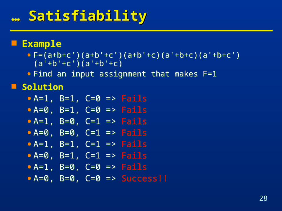
… … SatisfiabilitySatisfiability… … SatisfiabilitySatisfiability
Example• F=(a+b+c')(a+b'+c')(a+b'+c)(a'+b+c)(a'+b+c')(a'+b'+c')(a'+b'+c)
• Find an input assignment that makes F=1
Solution
• A=1, B=1, C=0 => Fails
• A=0, B=1, C=0 => Fails
• A=1, B=0, C=1 => Fails
• A=0, B=0, C=1 => Fails
• A=1, B=1, C=1 => Fails
• A=0, B=1, C=1 => Fails
• A=1, B=0, C=0 => Fails
• A=0, B=0, C=0 => Success!!
29
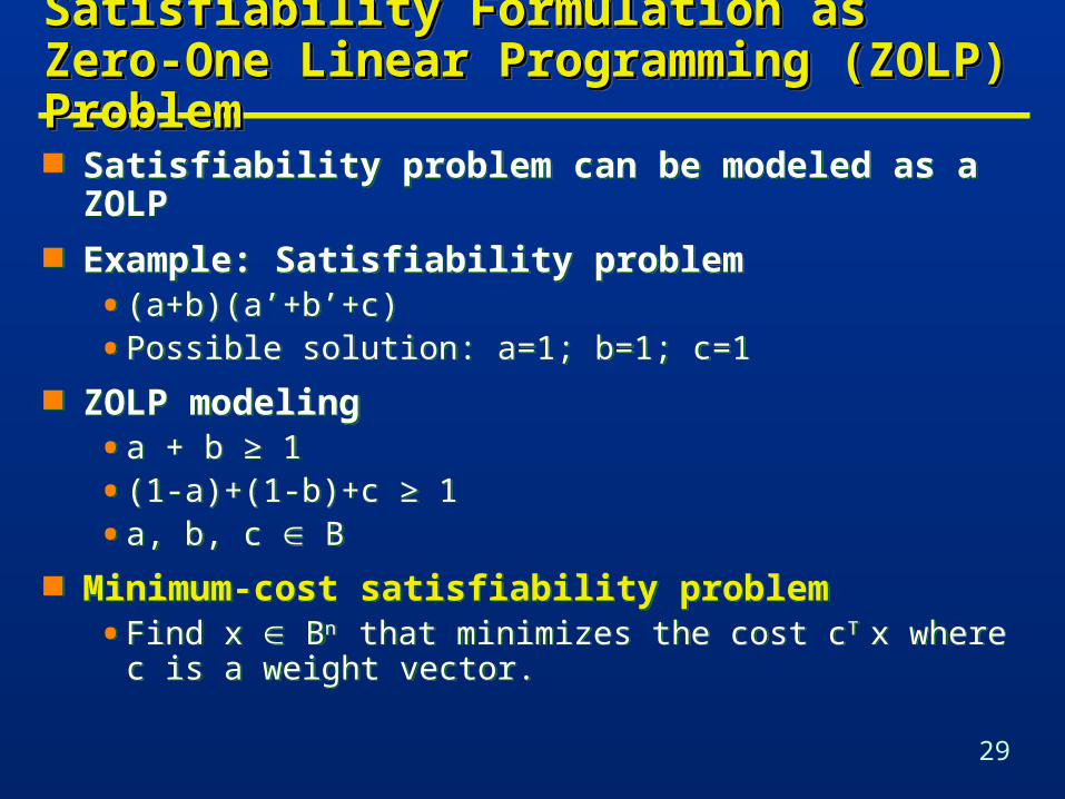
Satisfiability Formulation as Zero-One Satisfiability Formulation as Zero-One Linear Programming (ZOLP) ProblemLinear Programming (ZOLP) ProblemSatisfiability Formulation as Zero-One Satisfiability Formulation as Zero-One Linear Programming (ZOLP) ProblemLinear Programming (ZOLP) Problem
Satisfiability problem can be modeled as a ZOLP Example: Satisfiability problem
• (a+b)(a’+b’+c)
• Possible solution: a=1; b=1; c=1
ZOLP modeling• a + b ≥ 1
• (1-a)+(1-b)+c ≥ 1
• a, b, c B
Minimum-cost satisfiability problem• Find x Bn that minimizes the cost cT x where c is a weight
vector.
Satisfiability problem can be modeled as a ZOLP Example: Satisfiability problem
• (a+b)(a’+b’+c)
• Possible solution: a=1; b=1; c=1
ZOLP modeling• a + b ≥ 1
• (1-a)+(1-b)+c ≥ 1
• a, b, c B
Minimum-cost satisfiability problem• Find x Bn that minimizes the cost cT x where c is a weight
vector.
30
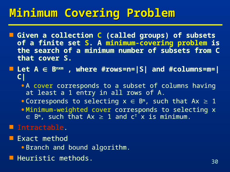
Minimum Covering Problem Minimum Covering Problem Minimum Covering Problem Minimum Covering Problem
Given a collection C (called groups) of subsets of a finite set S. A minimum-covering problem is the search of a minimum number of subsets from C that cover S.
Let A Bnxm , where #rows=n=|S| and #columns=m=|C|• A cover corresponds to a subset of columns having at least a
1 entry in all rows of A.
• Corresponds to selecting x Bm, such that Ax 1
• Minimum-weighted cover corresponds to selecting x Bm, such that Ax 1 and cT x is minimum.
Intractable. Exact method
• Branch and bound algorithm.
Heuristic methods.
31
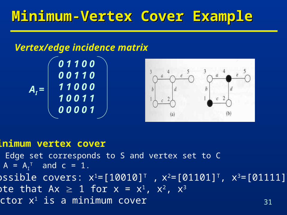
Minimum-Vertex Cover ExampleMinimum-Vertex Cover ExampleMinimum-Vertex Cover ExampleMinimum-Vertex Cover Example
0 1 1 0 00 0 1 1 01 1 0 0 01 0 0 1 10 0 0 0 1
AI =
Vertex/edge incidence matrix
• Minimum vertex cover • Edge set corresponds to S and vertex set to C• A = AI
T and c = 1.
• Possible covers: x1=[10010]T , x2=[01101]T, x3=[01111]T • Note that Ax 1 for x = x1, x2, x3
• Vector x1 is a minimum cover
32
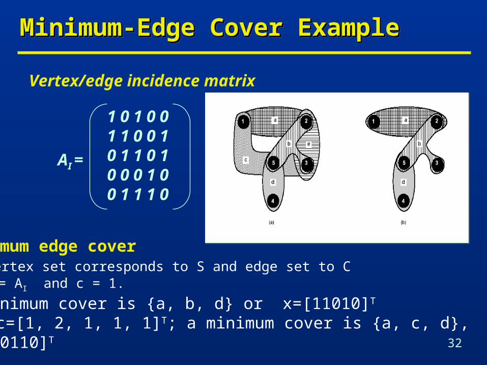
Minimum-Edge Cover ExampleMinimum-Edge Cover ExampleMinimum-Edge Cover ExampleMinimum-Edge Cover Example
1 0 1 0 01 1 0 0 10 1 1 0 10 0 0 1 00 1 1 1 0
AI =
Vertex/edge incidence matrix
• Minimum edge cover • Vertex set corresponds to S and edge set to C• A = AI and c = 1.
• A minimum cover is {a, b, d} or x=[11010]T
• Let c=[1, 2, 1, 1, 1]T; a minimum cover is {a, c, d}, x=[10110]T
33
Covering Problem Formulated as Covering Problem Formulated as Satisfiability ProblemSatisfiability ProblemCovering Problem Formulated as Covering Problem Formulated as Satisfiability ProblemSatisfiability Problem
Associate a selection variable with each group (element of C)
Associate a clause with each element of S• Each clause represents those groups that can cover the
element
• Disjunction of variables corresponding to groups
Note that the product of clauses is a unate expression• Unate cover
Edge-cover example• (x1+x3)(x1+x2+x5)(x2+x3+x5)(x4)(x2+x3+x4)=1
• (x1+x3) denotes vertex v1 must be covered by edge a or c
• x=[11010]T satisfies the product of sums expression
34
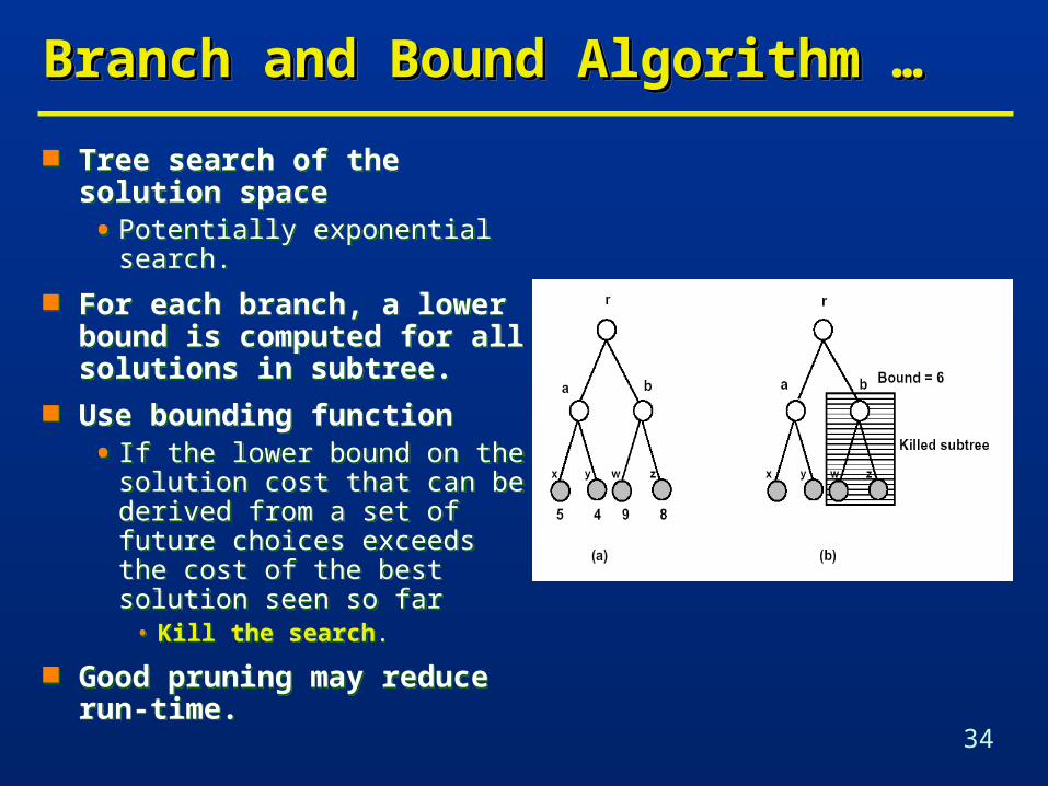
Branch and Bound Algorithm …Branch and Bound Algorithm …Branch and Bound Algorithm …Branch and Bound Algorithm …
Tree search of the solution space• Potentially exponential search.
For each branch, a lower bound is computed for all solutions in subtree.
Use bounding function• If the lower bound on the
solution cost that can be derived from a set of future choices exceeds the cost of the best solution seen so far
• Kill the search.
Good pruning may reduce run-time.
35
… … Branch and Bound AlgorithmBranch and Bound Algorithm… … Branch and Bound AlgorithmBranch and Bound Algorithm
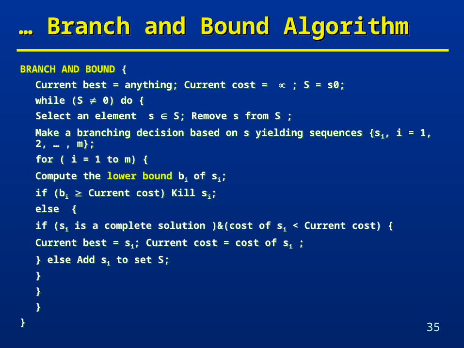
BRANCH AND BOUND {
Current best = anything; Current cost = ; S = s0;
while (S 0) do {
Select an element s S; Remove s from S ;
Make a branching decision based on s yielding sequences {si, i = 1, 2, … , m};
for ( i = 1 to m) {
Compute the lower bound bi of si;
if (bi Current cost) Kill si;
else {
if (si is a complete solution )&(cost of si < Current cost) {
Current best = si; Current cost = cost of si ;
} else Add si to set S;
}
}
}
}
36
Covering Reduction Strategies …Covering Reduction Strategies …Covering Reduction Strategies …Covering Reduction Strategies …
Partitioning• If A is block diagonal
• Solve covering problem for corresponding blocks.
Essentials• Column incident to one (or more) rows with single 1
• Select column.• Remove covered row(s) from table.
Column dominance
• If aki akj k: remove column j.
• dominating column covers more rows
Row dominance
• If aik ajk k : Remove row i.
• A cover for the dominated rows is a cover for the set
37
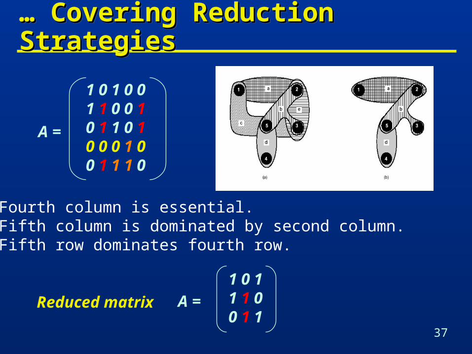
… … Covering Reduction StrategiesCovering Reduction Strategies… … Covering Reduction StrategiesCovering Reduction Strategies
1 0 1 0 01 1 0 0 10 1 1 0 10 0 0 1 00 1 1 1 0
A =
• Fourth column is essential.• Fifth column is dominated by second column.• Fifth row dominates fourth row.
1 0 11 1 00 1 1
A =Reduced matrix
38
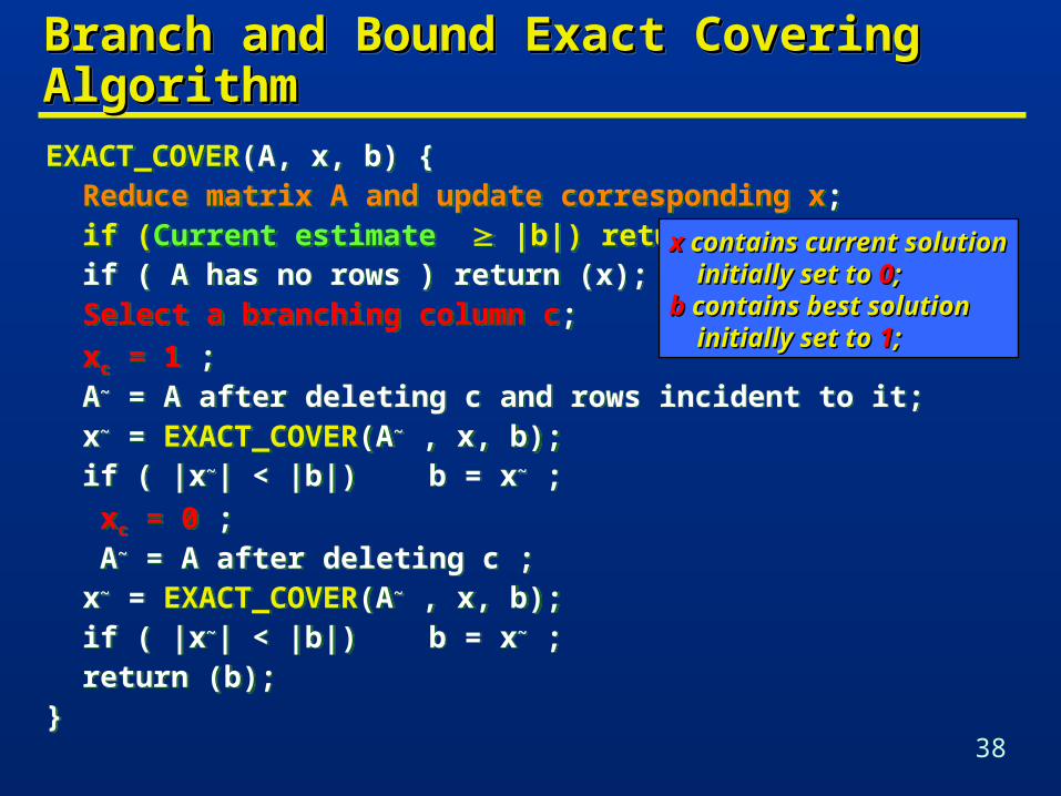
Branch and Bound Exact Covering Branch and Bound Exact Covering AlgorithmAlgorithmBranch and Bound Exact Covering Branch and Bound Exact Covering AlgorithmAlgorithm
EXACT_COVER(A, x, b) {Reduce matrix A and update corresponding x;if (Current estimate |b|) return(b);if ( A has no rows ) return (x);Select a branching column c;
xc = 1 ;A~ = A after deleting c and rows incident to it;x~ = EXACT_COVER(A~ , x, b);if ( |x~| < |b|) b = x~ ;
xc = 0 ; A~ = A after deleting c ;x~ = EXACT_COVER(A~ , x, b);if ( |x~| < |b|) b = x~ ;return (b);
}
xx contains current solution contains current solution initially set to initially set to 00;;b b contains best solutioncontains best solution initially set to initially set to 11;;
39
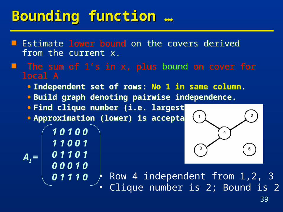
Bounding function …Bounding function …Bounding function …Bounding function …
Estimate lower bound on the covers derived from the current x.
The sum of 1’s in x, plus bound on cover for local A• Independent set of rows: No 1 in same column.
• Build graph denoting pairwise independence.
• Find clique number (i.e. largest clique)
• Approximation (lower) is acceptable.
Estimate lower bound on the covers derived from the current x.
The sum of 1’s in x, plus bound on cover for local A• Independent set of rows: No 1 in same column.
• Build graph denoting pairwise independence.
• Find clique number (i.e. largest clique)
• Approximation (lower) is acceptable.
• Row 4 independent from 1,2, 3• Clique number is 2; Bound is 2
1 0 1 0 01 1 0 0 10 1 1 0 10 0 0 1 00 1 1 1 0
AI =
40
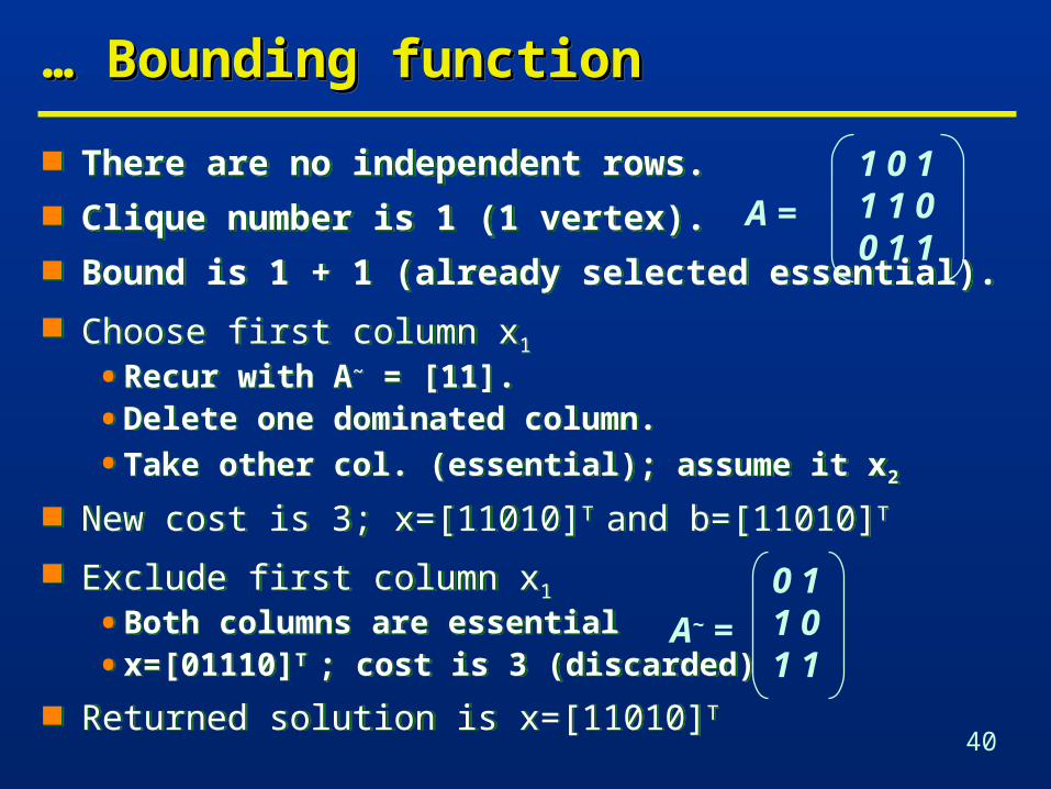
… … Bounding functionBounding function… … Bounding functionBounding function
There are no independent rows. Clique number is 1 (1 vertex). Bound is 1 + 1 (already selected essential).
Choose first column x1
• Recur with A~ = [11].
• Delete one dominated column.
• Take other col. (essential); assume it x2
New cost is 3; x=[11010]T and b=[11010]T
Exclude first column x1
• Both columns are essential
• x=[01110]T ; cost is 3 (discarded)
Returned solution is x=[11010]T
0 11 01 1
A~ =
1 0 11 1 00 1 1
A =