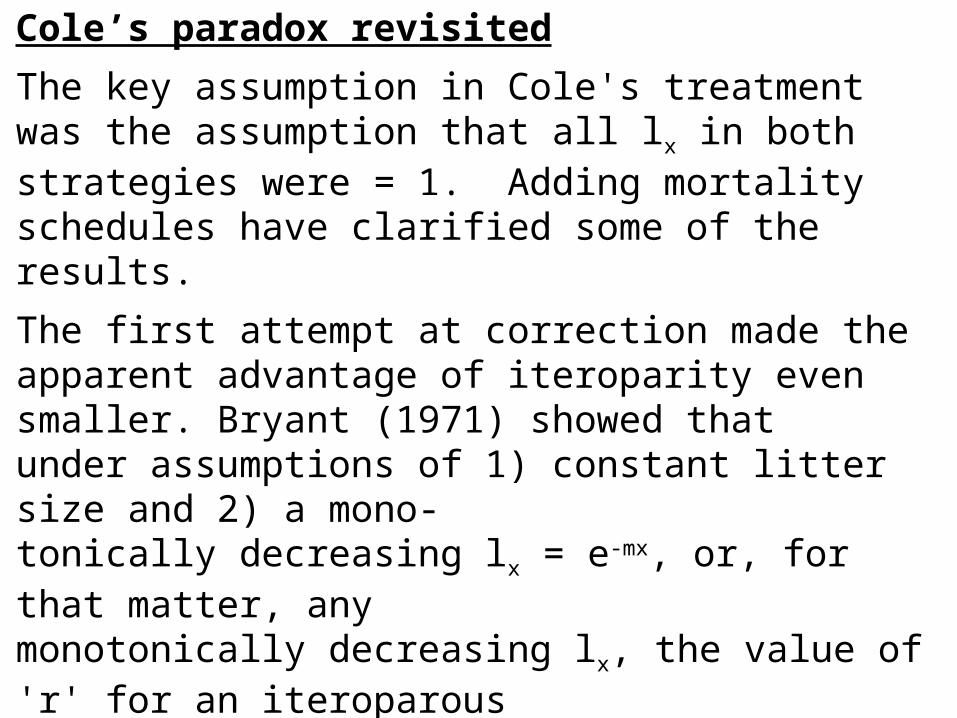
Cole’s paradox revisited

The key assumption in Cole's treatment was the assumption that all lx in both strategies were = 1. Adding mortality schedules have clarified some of the results.

The first attempt at correction made the apparent advantage of iteroparity even smaller. Bryant (1971) showed that under assumptions of 1) constant litter size and 2) a mono-tonically decreasing lx = e-mx, or, for that matter, any monotonically decreasing lx, the value of 'r' for an iteroparous species is not even increased as much as by adding 1 to the semelparous litter size.

However, a second attempt was both more ‘realistic’ and more successful.

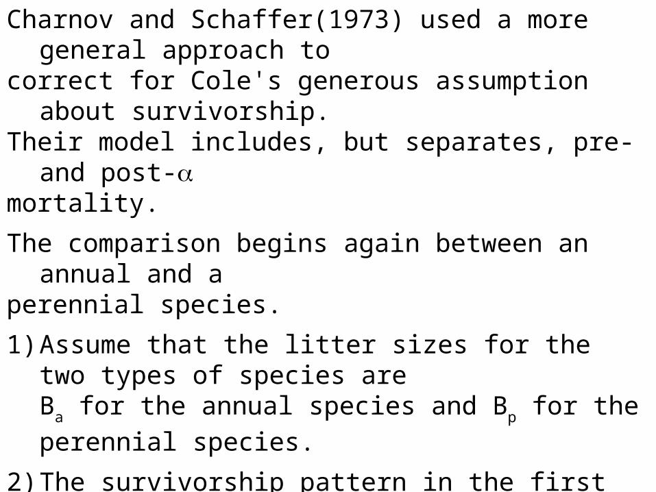
Charnov and Schaffer(1973) used a more general approach to correct for Cole's generous assumption about survivorship. Their model includes, but separates, pre- and post-mortality.

The comparison begins again between an annual and a perennial species.

1) Assume that the litter sizes for the two types of species are Ba for the annual species and Bp for the perennial species.

2) The survivorship pattern in the first year is l1 = C for both

types. Following reproduction in the first year, the semelparous species dies, and the perennial species continues with an annual proportional survivorship px = P.

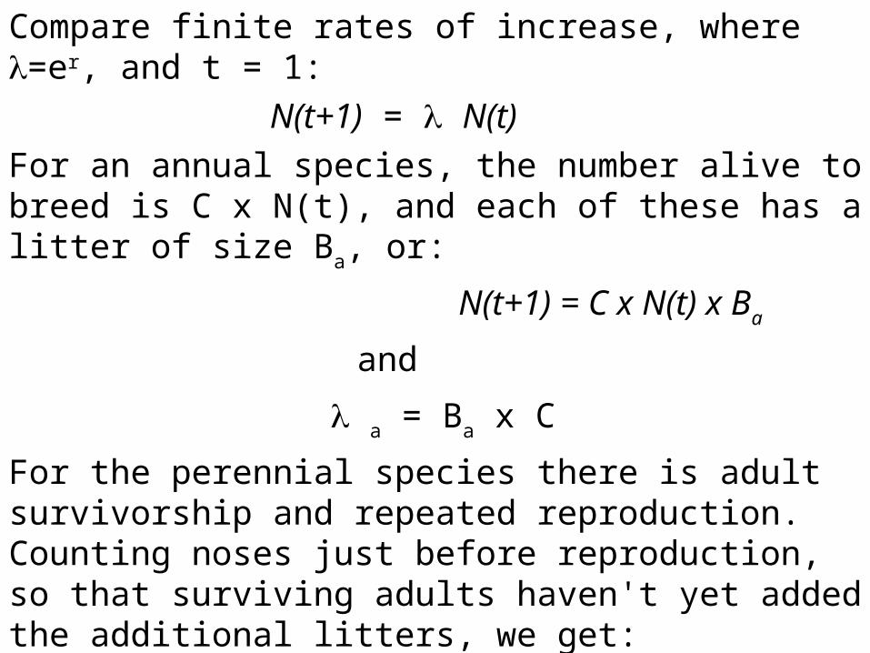
Compare finite rates of increase, where =er, and t = 1:

N(t+1) = N(t) 

For an annual species, the number alive to breed is C x N(t), and each of these has a litter of size Ba, or:

N(t+1) = C x N(t) x Ba

and

a = Ba x C

For the perennial species there is adult survivorship and repeated reproduction. Counting noses just before reproduction, so that surviving adults haven't yet added the additional litters, we get:

N(t+1) = Bp x C x N(t) + P x N(t)

and p = Bp x C + P

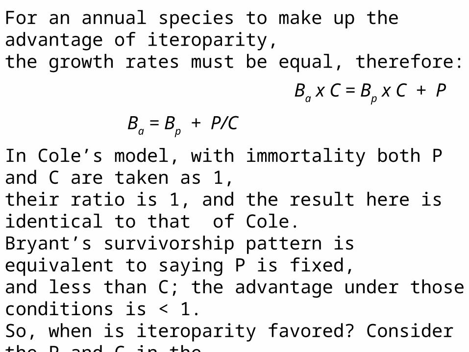
For an annual species to make up the advantage of iteroparity, the growth rates must be equal, therefore:

Ba x C = Bp x C + P

Ba = Bp + P/C

In Cole’s model, with immortality both P and C are taken as 1, their ratio is 1, and the result here is identical to that of Cole.Bryant’s survivorship pattern is equivalent to saying P is fixed, and less than C; the advantage under those conditions is < 1.So, when is iteroparity favored? Consider the P and C in the three Deevey survivorship patterns:

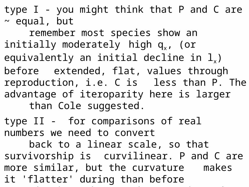
type I - you might think that P and C are ~ equal, but remember most species show an initially moderately high qx, (or equivalently an initial decline in lx) before extended, flat, values through reproduction, i.e. C is less than P. The advantage of iteroparity here is larger than Cole suggested.

type II - for comparisons of real numbers we need to convert back to a linear scale, so that survivorship is

curvilinear. P and C are more similar, but the curvature makes it 'flatter' during than before reproduction. The advantage is ~ what Cole calculated.

type III - its obvious that P is far larger than C, the early part of the curve is very steep, and the curve is relatively flat through reproduction. The advantage of iteroparity is far larger than Cole’s suggestion.

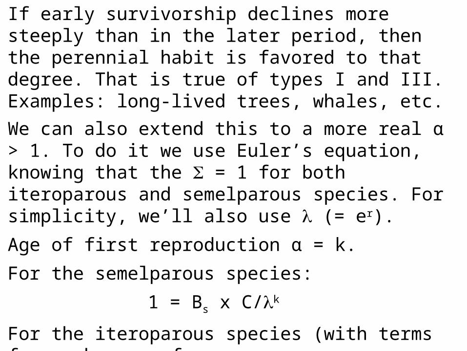
If early survivorship declines more steeply than in the later period, then the perennial habit is favored to that degree. That is true of types I and III. Examples: long-lived trees, whales, etc.

We can also extend this to a more real α > 1. To do it we use Euler’s equation, knowing that the = 1 for both iteroparous and semelparous species. For simplicity, we’ll also use (= er).

Age of first reproduction α = k.

For the semelparous species:

1 = Bs x C/k

For the iteroparous species (with terms for each year of reproduction, beginning with age k):

1 = Bi x C [1/k + P/ k+1 + P2/k+2 + …]

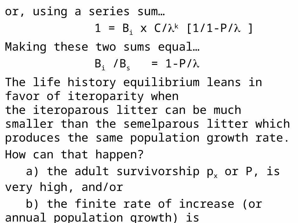
or, using a series sum…

1 = Bi x C/k [1/1-P/ ]

Making these two sums equal…

Bi /Bs = 1-P/

The life history equilibrium leans in favor of iteroparity whenthe iteroparous litter can be much smaller than the semelparous litter which produces the same population growth rate.

How can that happen?

a) the adult survivorship px or P, is very high, and/or

b) the finite rate of increase (or annual population growth) is very low.

Cole’s graph showed us (with the restrictions of his assumptions) that the higher the adult proportional survivorship the more the advantage to be gained from iteroparity, since that means many more litters will be produced over the lifespan. It also showed that the advantage grew as litters decreased in size.

The terms and quantitative advantages are different in the more realistic approach (no immortality, at least), but the basic result is identical, even in terms of the life history patterns that affect advantage.

An Energetics View of Iteroparity vs. Semelparity

The various approaches used by Cole and and others to testthe advantage of iteroparity are all based on comparison ofpopulation growth rates; they do not consider the position of the individual committed to a strategy. A final view of the contrast between iteroparity and semelparity, and when each should be expected, considers instead the energetics of the reproducing organism.

A surprising amount of modern ecological theory has come from application and/or adaptation of ideas from economics. One of those is the use of cost-benefit analyses to assess strategies.

Gadgil and Bossert (1970) used cost/benefit analysis to suggest patterns which lead to iteroparity. At any age the amount of reproductive effort which should be expended is determined by balancing the profit gained by reproduction (measured as the reproductive value at that age against the costs inevitably incurred.

To compare all possibilities, Gadgil and Bossert defined 3 shapes of profit and cost functions to be plotted against reproductive effort. The 3 kinds of curves are concave, linear and convex.

We’ll consider some examples:

Consider an example: cost and profit functions for reproduction in migrating salmonids -

The initial effort required to spawn even one egg is the enormous cost of migration from deep ocean to upstream fresh water. Thus the curve rises very sharply at low reproductive effort. However, the additional cost to spawn more eggs is basically the metabolic cost of the egg tissue, that is much more modest and basically flat (i.e. each egg costs about the same amount, independent of how many have been already formed).

The profit from increases in reproductive effort, i.e. the number of offspring, increases at least in direct proportion to the number of eggs. Schooling or other advantages of offspring groups might make the profit curve not linear, but slightly concave.

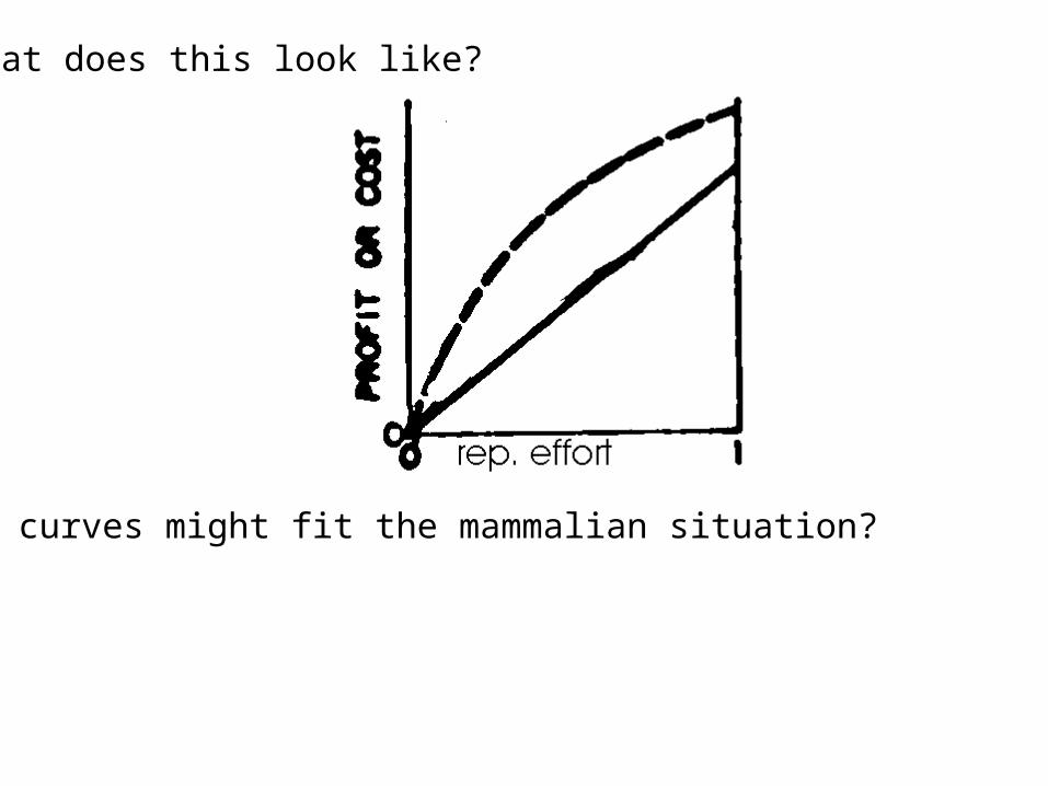
What does this look like?

Which curves might fit the mammalian situation?

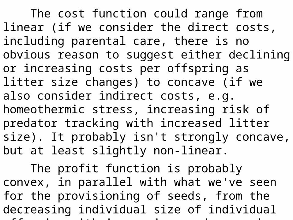
The cost function could range from linear (if we consider the direct costs, including parental care, there is no obvious reason to suggest either declining or increasing costs per offspring as litter size changes) to concave (if we also consider indirect costs, e.g. homeothermic stress, increasing risk of predator tracking with increased litter size). It probably isn't strongly concave, but at least slightly non-linear.

The profit function is probably convex, in parallel with what we've seen for the provisioning of seeds, from the decreasing individual size of individual offspring with increasing seed crop size. Again, the curvature is probably not dramatic, at least in homeothermic animals (birds, mammals) since homeothermy leads to some sharing of warmth among members of a brood, and also sharing of teats, which limits food intake no matter how hard the mother works.

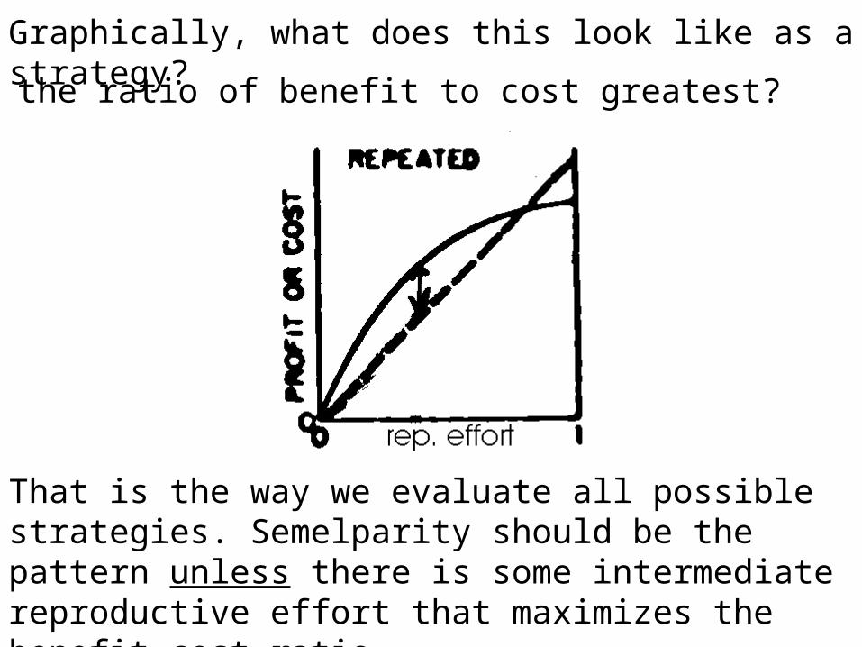
Graphically, what does this look like as a strategy?

Where is the ratio of benefit to cost greatest?

That is the way we evaluate all possible strategies. Semelparity should be the pattern unless there is some intermediate reproductive effort that maximizes the benefit-cost ratio.

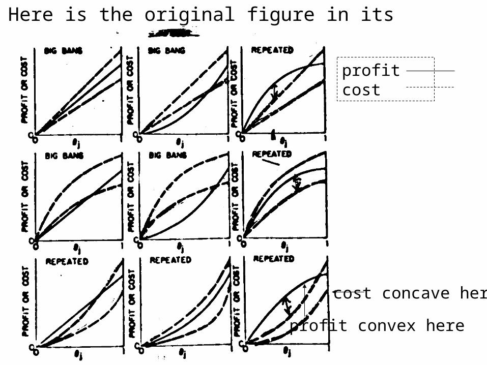
Here is the original figure in its entirety…

profit cost

profit convex here

cost concave here

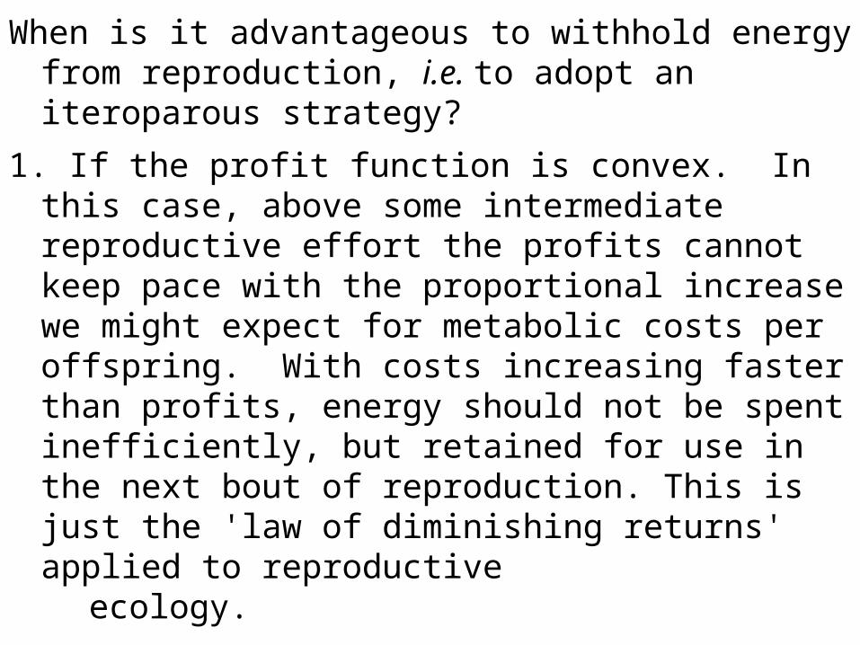
When is it advantageous to withhold energy from reproduction, i.e. to adopt an iteroparous strategy?

1.  If the profit function is convex. In this case, above some intermediate reproductive effort the profits cannot keep pace with the proportional increase we might expect for metabolic costs per offspring. With costs increasing faster than profits, energy should not be spent inefficiently, but retained for use in the next bout of reproduction. This is just the 'law of diminishing returns' applied to reproductive

ecology.

The efficiency argument even applies when the ratio remains constant. For that, the middle case, the total number of offspring produced from a given amount of energy can be maximized by reducing reproductive effort, even if benefit-cost ratio has no maximization.

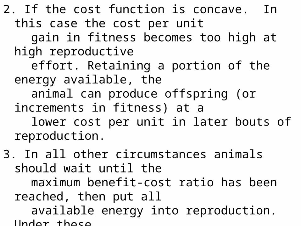
2. If the cost function is concave. In this case the cost per unit gain in fitness becomes too high at high reproductive effort. Retaining a portion of the energy available, the animal can produce offspring (or increments in fitness) at a lower cost per unit in later bouts of reproduction.

3. In all other circumstances animals should wait until the maximum benefit-cost ratio has been reached, then put all available energy into reproduction. Under these circumstances the semelparity is optimum. That includes the case where profit and cost are both linear. There is no change in cost per unit with effort,and we now know the advantage of early reproduction. There is no advantage to

restraint, especially given survivorship factors

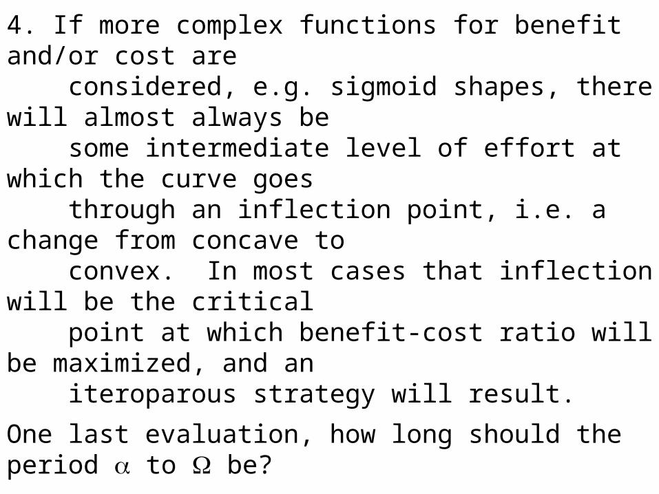
4. If more complex functions for benefit and/or cost are considered, e.g. sigmoid shapes, there will almost always be some intermediate level of effort at which the curve goes through an inflection point, i.e. a change from concave to convex. In most cases that inflection will be the critical point at which benefit-cost ratio will be maximized, and an iteroparous strategy will result.

One last evaluation, how long should the period to be?

That depends on the security of survivorship (px), and on the

variability in reproductive success. If survival is relatively assured, no single bout of reproduction is under severe pressure to produce success. Else, if survivorship is low or variable, then the pressure for success from any single bout (or a few) is much higher, and more effort (and a shorter - is likely.

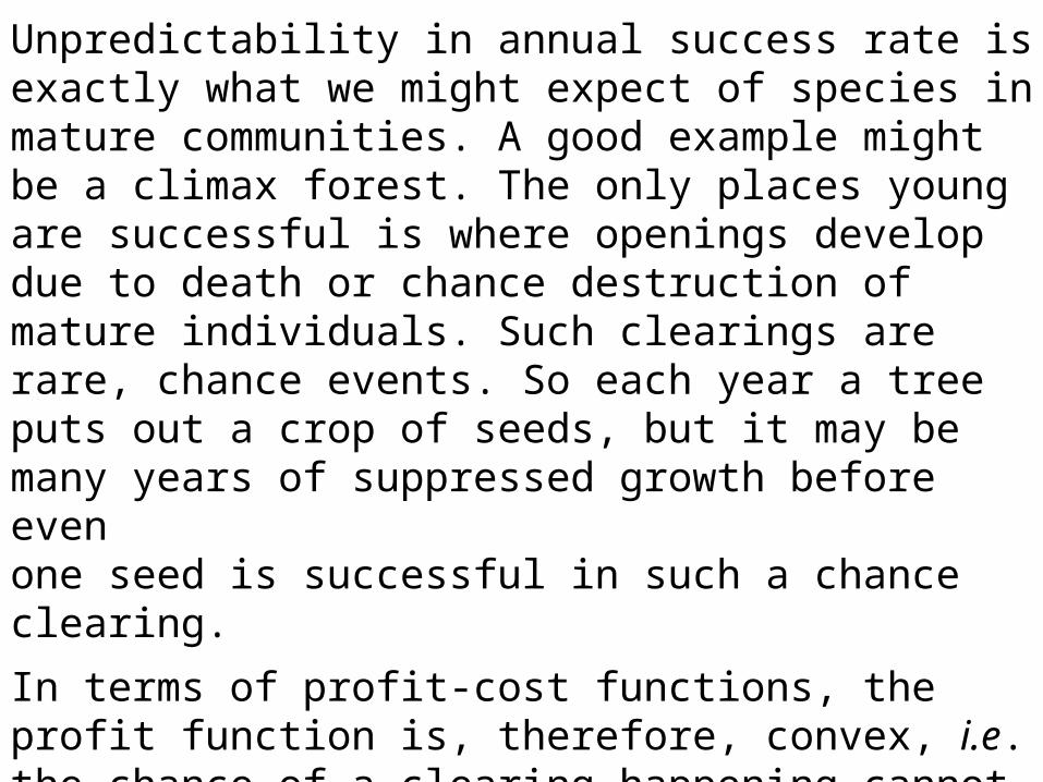
Unpredictability in annual success rate is exactly what we might expect of species in mature communities. A good example might be a climax forest. The only places young are successful is where openings develop due to death or chance destruction of mature individuals. Such clearings are rare, chance events. So each year a tree puts out a crop of seeds, but it may be many years of suppressed growth before even one seed is successful in such a chance clearing.

In terms of profit-cost functions, the profit function is, therefore, convex, i.e. the chance of a clearing happening cannot be missed, so its necessary to put out a seed crop each year, but little advantage in putting out a huge crop. Instead, energy is retained to improve survivorship and make possible a larger number of seed crops.

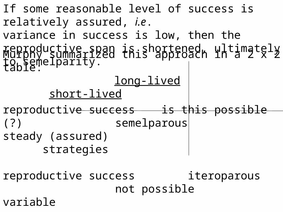
If some reasonable level of success is relatively assured, i.e.variance in success is low, then the reproductive span is shortened, ultimately to semelparity.

Murphy summarized this approach in a 2 x 2 table: long-lived short-lived

reproductive success is this possible (?) semelparoussteady (assured) strategies

reproductive success iteroparous not possiblevariable

The upper right hand box, semelparous strategies, is a necessary result of the association of lx and mx. If a species is short-lived, quantifiable as a small e0, then the only pattern to reproduction which will permit persistence is steady, assured success. Else, extinction will follow.

The lower, right hand box is also simply explained. This is what happens to a short-lived species does not have assured success. Extinction is the inevitable result when a species attempts reproduction only once (or possibly a few times) while the variability in reproductive success is high. That variability ensures that at some time a few bad years will follow in succession, and prevent an entire mature population from producing any surviving offspring, i.e. local extinction.

The closest real species come to this is to have facultative(that is have the potential for) dormancy in offspring. In this way the low survivorship of parents and low annual success in offspring can be mitigated through appearance of offspring (release from dormancy) when chances of offspring success are high.

In terms of the success of offspring, rather than annual success rates, this strategy becomes a special case of the upper right hand box, short adult life, but predictable offspring success. This strategy is fairly common in weeds, whose seeds may remain dormant for >100 years, and in some desert plants.

The box in the upper left has a ?. There are a number of approaches to indicate why that box should not be occupied by observed reproductive strategies. The most intuitive of them considers the effect of such a strategy on species interactions. This is a species which is long-lived and has predictable reproductive success. That should make this population very successful.

If the species in question is a prey item, its predator will evolve to more extensively utilize a species which is predictable, either through numerical or functionalresponses. The result of increased predation on this prey, whose life history we are following, will be either a reduced lifespan or greater variability in reproductive success.The effective result is to move the strategy for the species out of the ? box and into either of the more usual strategies.

Example(s) of this move:

A number of long-lived trees (apple trees are an example of one kind of response) have variable reproductive success; some years a heavy seed crop is produced (so-called mast years) and in other years the crop is much smaller.

This can be considered an adaptation to restrict insect (or other) herbivores by starvation, though it can also be a necessary response to energetic demands of reproduction. In this latter sense, it is a cost of reproduction. Having reproduced heavily in one year, the 'cost' is a very restricted reproduction in the following year.

There are always a variety of explanations for a pattern. Variability in reproductive success has also been used as an explanation for the strategy called ‘bet-hedging’. If there is variation in reproductive effort and success, and if reproductive effort and adult survivorship trade-off, then it pays to reduce reproductive effort in order to live longer and reproduce more times. Here’s a way of plotting that for bird clutches (sorry, plant plot unavailable):

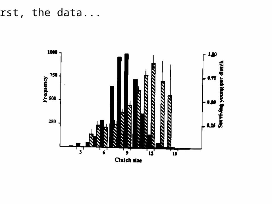
First, the data...

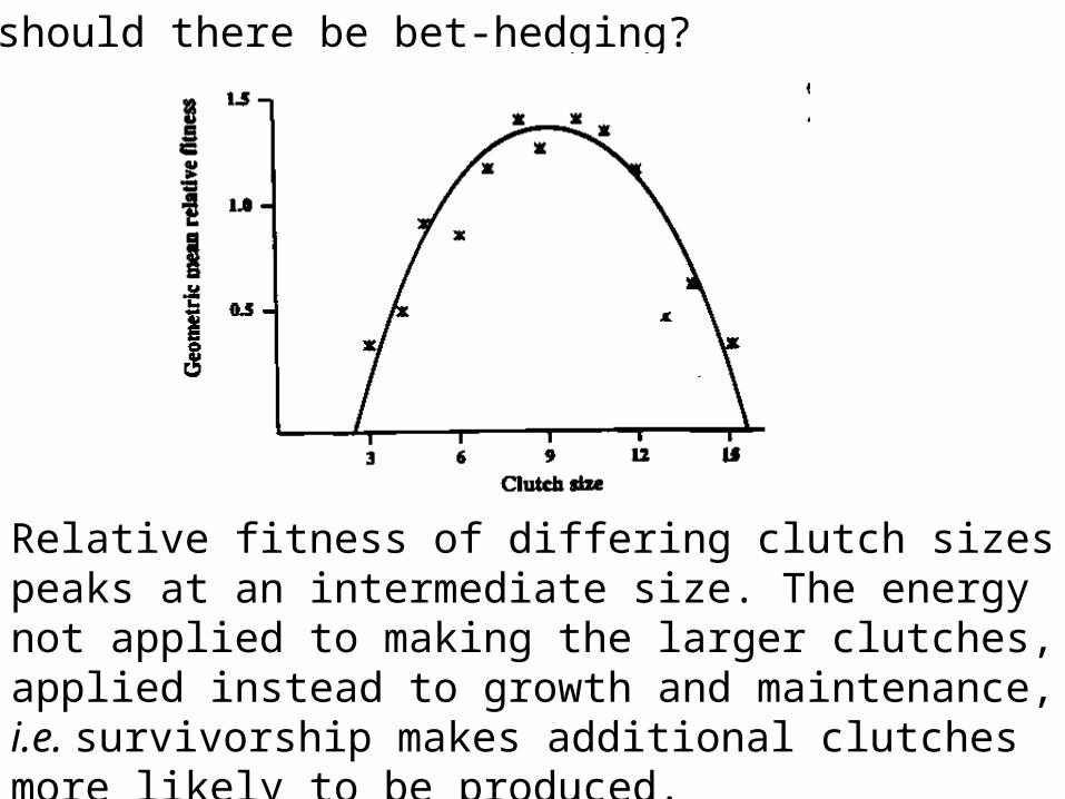
Why should there be bet-hedging?

Relative fitness of differing clutch sizes peaks at an intermediate size. The energy not applied to making the larger clutches, applied instead to growth and maintenance, i.e. survivorship makes additional clutches more likely to be produced.