Collective Experimentation: A Laboratory Study

Mikhail Freer, César Martinelli, and Siyu Wang

January 2018

Discussion Paper

Interdisciplinary Center for Economic Science 4400 University Drive, MSN 1B2, Fairfax, VA 22030 Tel: +1-703-993-4719 Fax: +1-703-993-4851 ICES Website: http://ices.gmu.edu ICES RePEc Archive Online at: http://edirc.repec.org/data/icgmuus.html

Collective Experimentation: A Laboratory Study

Mikhail Freer⇤ Cesar Martinelli† Siyu Wang‡

January 5, 2018

Abstract

We develop a simple model of collective experimentation and take it to the lab. In

equilibrium, as in the recent work of Strulovici (2010), majority rule has a bias toward

under experimentation, as good news for a minority of voters may lead a majority of

voters to abandon a policy when each of them thinks it is likely that the policy will be

passed by a future majority excluding them. We compare the behavior in the lab of

groups under majority rule and under the optimal voting rule, which precludes voting

in intermediate stages of the policy experiment. Surprisingly, performs better than the

(theoretically) optimal voting rule. Majority rule seems to be more robust than other

forms of voting when players make mistakes.

1 Introduction

Groups and societies often face decisions whose consequences for di↵erent individuals are

uncertain and can only be learn over time. As an illustration, trade reforms, changes in

immigration or environmental policies, big overhauls of the public health or the tax system,

etc. often have consequences that are heterogenous and hard to forecast for di↵erent indi-

viduals. Policy innovation in those circumstances is akin to an experiment conducted by the

society which may result in the new policies being entrenched or abandon as new evidence

mounts up. Such experiments open a new dimension to the collective choice problem, since

majority preferences in favor or against the new policies may change over time. In order

for the society to make decisions, it is necessary to specify not only a voting rule but also

how this rule is going to change over time. In this paper, we develop a simple model of the

dynamic collective experimentation problem. We use lab evidence to explore the e�ciency

⇤Department of Economics, University of Leuven (KU Leuven).

†Interdisciplinary Center for Economic Science at George Mason University.

‡Ford Motor Company.

1

implications of di↵erent dynamic voting rules from a utilitarian perspective, and to compare

game theoretic predictions with the behavior of subjects in the lab.

In the model, group members must decide whether to adopt or not a policy. It is unclear

ex ante who will benefit and who will lose from the policy. Individuals may learn that

they will win from the reform in two subsequent stages, after which they have to decide

whether to stick to the policy for good or abandon it. As in Strulovici’s (2010) influential

contribution, the policy may be derailed in an intermediate stage if a minority learns that

they will be winners, as voters in the remainder may anticipate the policy could be adopted

in the final stage even if they emerge individually as losers. In the context of the model,

the optimal voting rule specifies unanimity at intermediate stages and simple majority in

the final stage. The lab implementation reveals, surprisingly, that adopting simple majority

throughout yields more e�cient outcomes than the (game theoretic) optimal voting rule.

The reason is that simple majority is more robust to individual voters making mistakes in

a dynamic sense: the majority at the intermediate stage may derail policies that could be

adopted later on for good by a di↵erent majority by mistake. We also investigate whether

the bias toward overoptimism may be due to persistent versus temporary overoptimism, and

present evidence consistent with the latter.

The e�ciency advantages of unanimity versus simple majority is, of course, a classi-

cal theme in political economy, at least since the publication of the Calculus of Consent

(Buchanan and Tullock, 1962). To the traditional trade-o↵, predicated in a static setting,

our work adds a dynamic dimension. Evidence from the lab indicates that repeated major-

ity voting is self-correcting in a way that is not captured by equilibrium analysis. In our

setting, majority voting at an intermediate stage allows to overcome an overoptimism bias.

Subjects’ voting behavior is consistent with them overestimating their probability of success

after failing to receive high signals.

There is by now a growing theoretical literature on collective experimentation problems.

Fernandez and Rodrik (1991) provide the seminal contribution, showing that a policy may

have minority support ex ante even if it will have majority support ex post for sure if indi-

vidual voters are afraid of ending up in the losing minority. The above-mentioned article by

Strolovici models collective experimentation as a continuous time game with a continuum

of voters, identifies the deviations from e�ciency implied by adopting majority voting at

every moment and derives the (time contingent) optimal voting rule. Our model recovers

the strategic elements of Strulovici’s (2010) model in a discrete time setting with few voters

in a way that can be taken to the lab. This allows to check whether the strategic incen-

tives identified by the literature operate in a controlled setting, and explore deviations from

equilibrium predictions and their consequences.

Other recent theoretical work on collective experimentation has focused on collective

2

search by committees, as in the work of Albrech et al. (2010) and Moldovanu and Shi (2013),

on optimal voting rules for two period models, as in the work of Messner and Polborn

(2012), on incentives to over-experiment for preemptive reasons when the policymaker may

not remain in power, as in Callander and Hummel (2014), on dynamic sequential acquisition

by committees, as in Chan et al. (2015), and on extending Strolovici’s model to consider bad

signals, as in Khromenkova (2017). In spite of the growing interest and relevance of this line

of work, we are not aware of other lab research on dynamic collective experimentation.

The remainder of this paper organized as follows. Section 2 presents the simple collective

experimentation model we use and provides theoretical predictions. Section 3 provides details

about the experimental design. Section 4 presents results obtained from the experiment.

Section 5 gathers final remarks. All omitted proofs are collected in the Appendix.

2 Theoretical framework

We consider a simple three period voting game with three players in which players choose

between a safe and a risky project. Players can be of two types: high or low, depending on

whether the player receives a high (h) or a low (l) payo↵ if the risky project is implemented.

All players receive a payo↵ of s if the safe project is implemented, independently of type,

where h > s > l.

In the first period, players vote on whether to start experimenting or not. If they start

experimenting, each player receives a public signal. The signal can be high or uncertain.

If the player receives the high signal, then the player’s payo↵ from implementing the risky

project is h. If the signal is uncertain, the player does not know which payo↵ the player

would receive in case of implementing the risky project. If the player is of high type, then

there is a probability q 2 (0, 1) that the player will receive the high signal, while if the player

is of low type, there is a probability of zero that the player will receive a high signal.

In the second period, after observing the public signals received by all players, players

vote on whether to continue experimenting. If they continue, they receive signals again. For

notational simplicity, since their type has been already disclosed, we assume that players

who received high signals in period 1 receive them again in period 2. For the reminder of

players, as in the previous period, then there is a probability q 2 (0, 1) that the player will

receive the high signal, while if the player is of low type, there is a probability of zero that

the player will receive a high signal. We denote by wt 2 {0, 1, 2, 3} the total number of

“High” signals received in period t 2 {1, 2}, with w2 � w1 � 0.

Finally, in the third period, players vote on whether to implement the risky project or

the safe project. If the risky project is implemented, all voters’ types are disclosed; in either

case, all payo↵s are realized.

3

Denote by p0 the initial probability that the player is of a high type. Using Bayes’ Law,

the probability that a player is of high type after receiving an uncertain signal in period 1 is

p1 =p0(1� q)

1� p0q,

and the probability that a player is of high type after receiving uncertain signals in periods

1 and 2 is

p2 =p1(1� q)

1� p1q=

p0(1� q)2

1� 2p0q + p0q2.

We denote by

r = p2h+ (1� p2)l

the expected payo↵ from the risky project for a player that received uncertain signals in

periods 1 and 2. We assume r < s, so that a player that does not receive high signals would

prefer to adopt the safe project.

Note that a utilitarian social planner would experiment in periods 1 and 2, and would

adopt the project in the third period if w2h+(1�w2)r > 3s, and only if w2h+(1�w2)r � 3s.

We investigate the behavior of agents in the model under majority voting. We also

describe an optimal voting rule, i.e. a voting rule that implements the utilitarian social

planner’s choices. Our solution concept is Perfect Bayesian Equilibrium in undominated

strategies. As customary in voting games, we eliminate weakly dominated strategies to

avoid trivial equilibria in which no player is decisive. For notational simplicity, we assume

that players vote to continue experimenting when indi↵erent.

2.1 Majority voting and under experimentation

In this section, we provide conditions under which, in equilibrium, majority voting deviates

from the utilitarian social planner’s choices by stopping the policy after a minority gets good

news in period 1, but otherwise coincides with the social planner choices (see Figure 1).

Parameter values satisfying these restrictions allow us to test whether majority voting leads

to under experimentation as in Strulovici (2010).

We proceed by backward induction, from the last stage to the first. Since by assumption

h > s > r, in the third period only players who have obtained a high signal vote to implement

the policy, so the policy is implemented if w2 � 2. The condition in Lemma 1 below implies

that utilitarian social planner adopt the same decision than majority voting:

Lemma 1. The utilitarian social planner and majority voting outcomes coincide in the third

period if and only if1

2<

h� s

s� r< 2.

4

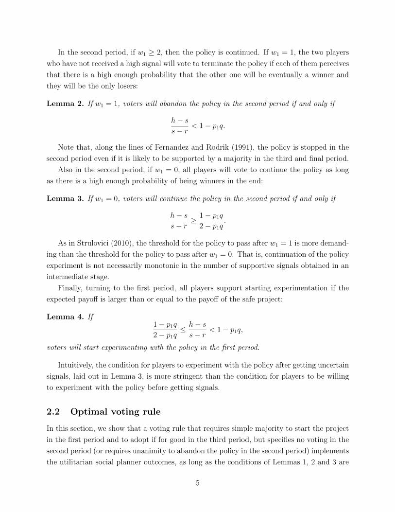
In the second period, if w1 � 2, then the policy is continued. If w1 = 1, the two players

who have not received a high signal will vote to terminate the policy if each of them perceives

that there is a high enough probability that the other one will be eventually a winner and

they will be the only losers:

Lemma 2. If w1 = 1, voters will abandon the policy in the second period if and only if

h� s

s� r< 1� p1q.

Note that, along the lines of Fernandez and Rodrik (1991), the policy is stopped in the

second period even if it is likely to be supported by a majority in the third and final period.

Also in the second period, if w1 = 0, all players will vote to continue the policy as long

as there is a high enough probability of being winners in the end:

Lemma 3. If w1 = 0, voters will continue the policy in the second period if and only if

h� s

s� r� 1� p1q

2� p1q.

As in Strulovici (2010), the threshold for the policy to pass after w1 = 1 is more demand-

ing than the threshold for the policy to pass after w1 = 0. That is, continuation of the policy

experiment is not necessarily monotonic in the number of supportive signals obtained in an

intermediate stage.

Finally, turning to the first period, all players support starting experimentation if the

expected payo↵ is larger than or equal to the payo↵ of the safe project:

Lemma 4. If1� p1q

2� p1q h� s

s� r< 1� p1q,

voters will start experimenting with the policy in the first period.

Intuitively, the condition for players to experiment with the policy after getting uncertain

signals, laid out in Lemma 3, is more stringent than the condition for players to be willing

to experiment with the policy before getting signals.

2.2 Optimal voting rule

In this section, we show that a voting rule that requires simple majority to start the project

in the first period and to adopt if for good in the third period, but specifies no voting in the

second period (or requires unanimity to abandon the policy in the second period) implements

the utilitarian social planner outcomes, as long as the conditions of Lemmas 1, 2 and 3 are

5

any

any

w2 � 2

Start

Continue

Implement

Stop

Stop

Stop

w1 = 1

w2 � 2

Start

Continue

Implement

Stop

Stop

Stop

(a) Social Planner (b) Majority Voting

Figure 1: Decision Trees

any

w2 � 2

Start

Continue

Implement

Stop

Stop

Stop

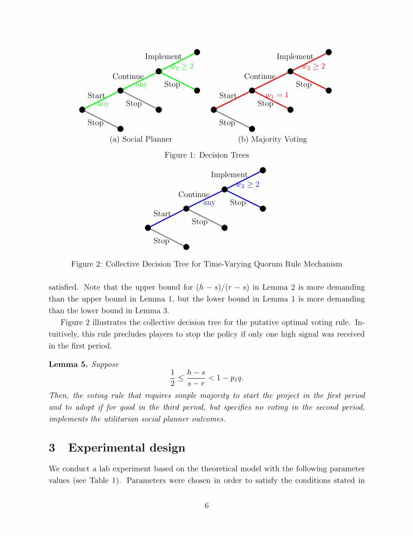
Figure 2: Collective Decision Tree for Time-Varying Quorum Rule Mechanism

satisfied. Note that the upper bound for (h � s)/(r � s) in Lemma 2 is more demanding

than the upper bound in Lemma 1, but the lower bound in Lemma 1 is more demanding

than the lower bound in Lemma 3.

Figure 2 illustrates the collective decision tree for the putative optimal voting rule. In-

tuitively, this rule precludes players to stop the policy if only one high signal was received

in the first period.

Lemma 5. Suppose1

2 h� s

s� r< 1� p1q.

Then, the voting rule that requires simple majority to start the project in the first period

and to adopt if for good in the third period, but specifies no voting in the second period,

implements the utilitarian social planner outcomes.

3 Experimental design

We conduct a lab experiment based on the theoretical model with the following parameter

values (see Table 1). Parameters were chosen in order to satisfy the conditions stated in

6

Lemmas 1, 2 and 3. Therefore, equilibrium behavior predicts that simple majority would be

suboptimal, while the optimal voting rule delivers outcomes that coincide with the utilitarian

planner choices.

Parameter ValueProbability of being high type p0 1/2Probability that signal reveals the type q 1/2High payo↵ h 500Low payo↵ l 50Safe payo↵ s 350Exchange rate 20 tokens per US dollar

Table 1: Parameters specification

The experimental design consists of two treatments. In the first treatment, subjects

make decisions under simple majority and in the second one under the optimal voting rule.

We refer to them as majority treatment and optimal treatment. The game was played 15

rounds with random reshu✏ing of the groups, to ensure that the were no repetitions with

the same group composition. The experiment was coded and conducted using oTree (Chen

et al., 2016). Experimental instructions can be found in the appendix. We conducted the

experiment with 60 undergraduate students from George Mason University. There were 36

subjects in the majority treatment and 24 in in the optimal treatment. Subjects’ earnings

varied between $10 and $40.

4 Experimental results

We start by looking at group level results to test theoretical predictions and compare the

performance of the two voting rules. Then we move on to analyzing individual behavior to

explore possible biases which caused the observed group level behavior. Finally, we present

results from the structural estimates of the Quantal Response Equilibrium model (introduced

by McKelvey and Palfrey, 1995, 1998).

4.1 Group level analysis

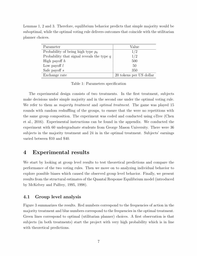
Figure 3 summarizes the results. Red numbers correspond to the frequencies of action in the

majority treatment and blue numbers correspond to the frequencies in the optimal treatment.

Green lines correspond to optimal (utilitarian planner) choices. A first observation is that

subjects (in both treatments) start the project with very high probability which is in line

with theoretical predictions.

7

t = 1 Nature t = 2 Nature t = 3

Start

Stop

w1 = 1

w1 = 0

w1 � 2

Stop

Continue

Stop

Continue

Stop

Continue

w2 = 0

w2 = 1

w2 � 2

w2 = 1

w2 � 2

w2 � 2

Stop

Implement

Stop

Implement

Stop

Implement

Stop

Implement

Stop

Implement

Stop

Implement

.04 .00

.13 .00

.28 .00

.41 .00

.951

[.83][1]

.78

.91[.64][.91]

.36

.39[.25][.39]

11

[.67][1]

.33

.37[.22][.37]

.05

.19[.03][.19]

.05 .00

.22 .09

.64 .61

.00 .00

.67 .63

.95 .87

Figure 3: Probabilities of abandoning and implementing the policy on the collective decisiontree. Red and Blue numbers correspond, respectively, to the frequencies obtained in themajority treatment and in the optimal treatment. Green lines correspond to the sociallyoptimal decisions at every node. Stopping frequencies and frequencies of policy implemen-tations displayed are conditional on the probability of reaching the node. In square bracketswe show probabilities of implementing the policy conditional only on the history of signalsreceived.

8

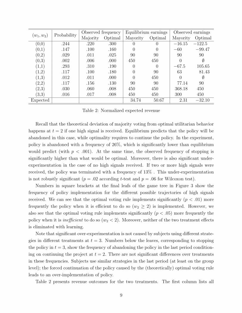
(w1, w2) ProbabilityObserved frequency Equilibrium earnings Observed earningsMajority Optimal Mayority Optimal Mayority Optimal

(0,0) .244 .220 .300 0 0 �16.15 �122.5(0,1) .147 .100 .160 0 0 �60 �99.47(0,2) .029 .011 .025 90 90 90 90(0,3) .002 .006 .000 450 450 0 ;(1,1) .293 .310 .190 0 0 �67.5 105.65(1,2) .117 .100 .180 0 90 63 81.43(1,3) .012 .011 .000 0 450 0 ;(2,2) .117 .156 .130 90 90 77.14 90(2,3) .030 .060 .008 450 450 368.18 450(3,3) .016 .017 .008 450 450 300 450

Expected 34.74 50.67 2.31 �32.10

Table 2: Normalized expected revenue

Recall that the theoretical deviation of majority voting from optimal utilitarian behavior

happens at t = 2 if one high signal is received. Equilibrium predicts that the policy will be

abandoned in this case, while optimality requires to continue the policy. In the experiment,

policy is abandoned with a frequency of 26%, which is significantly lower than equilibrium

would predict (with p < .001). At the same time, the observed frequency of stopping is

significantly higher than what would be optimal. Moreover, there is also significant under-

experimentation in the case of no high signals received. If two or more high signals were

received, the policy was terminated with a frequency of 13% . This under-experimentation

is not robustly significant (p = .02 according t-test and p = .06 for Wilcoxon test).

Numbers in square brackets at the final leafs of the game tree in Figure 3 show the

frequency of policy implementation for the di↵erent possible trajectories of high signals

received. We can see that the optimal voting rule implements significantly (p < .01) more

frequently the policy when it is e�cient to do so (w2 � 2) is implemented. However, we

also see that the optimal voting rule implements significantly (p < .05) more frequently the

policy when it is ine�cient to do so (w2 < 2). Moreover, neither of the two treatment e↵ects

is eliminated with learning.

Note that significant over-experimentation is not caused by subjects using di↵erent strate-

gies in di↵erent treatments at t = 3. Numbers below the leaves, corresponding to stopping

the policy in t = 3, show the frequency of abandoning the policy in the last period condition-

ing on continuing the project at t = 2. There are not significant di↵erences over treatments

in these frequencies. Subjects use similar strategies in the last period (at least on the group

level); the forced continuation of the policy caused by the (theoretically) optimal voting rule

leads to an over-implementation of policy.

Table 2 presents revenue outcomes for the two treatments. The first column lists all

9

possible signal histories for a group. The second one shows the theoretical probabilities with

which the history appears. The third and fourth columns show the observed frequencies for

every history by treatment. Note that there are deviations from theoretical probabilities in

both treatments, and there are di↵erences in frequencies between treatments. For compar-

ison purposes, we use theoretical probabilities instead of observed frequencies to compute

expected earnings for every treatment. The fifth and sixth columns show earning outcomes

for the group for every history derived from theoretical equilibrium behavior. The last two

columns show the averaged observed earning outcomes for every history. (The symbol ;denotes histories for which there is no observations and correspond to the zero observed

frequency events.). Revenue data is normalized by subtracting 1050 = 350⇥ 3 (revenue for

the group from the safe project). Hence, numbers in the last two columns indicate net gains

or loses from implementing the policy instead of the safe payo↵.

Expected observed revenue is higher in the majority rule treatment. This is caused

by significant over-experimentation in the optimal voting rule treatment. We conduct a

two-step bootstrapping procedure (see Appendix B for details) that confirms the statistical

significance of the di↵erences in expected net earnings presented in Table 2. Expected group

revenue under the optimal voting rule is in fact negative–the group is doing worse than

always staying with the safe payo↵. This is a consequence of both over implementation and

the fact that with our parameter specification most probability weight lies in the domain

where behavior under the optimal voting rule leads to ine�cient outcomes.

4.2 Individual level analysis

In the section we turn to the analysis of observed individual behavior. In particular, we

investigate possible behavioral biases causing observed group level results.

Recall that the equilibrium action in both treatments in the first period is to vote to

start the policy, and in the third period it is to vote to implement the policy for good in the

third period if a player has obtained a high signal, and against implementing the policy if

the player has not obtained a high signal. In the second period, in the majority treatment,

under our parameter specification, the equilibrium action is to vote to continue the policy if

a player has obtained a high signal or if no one else has obtained a high signal, and to vote

to abandon the policy otherwise.

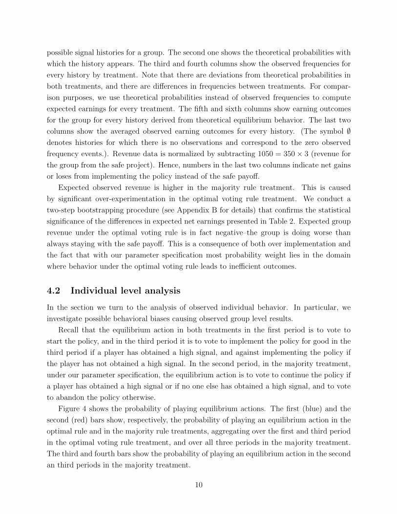
Figure 4 shows the probability of playing equilibrium actions. The first (blue) and the

second (red) bars show, respectively, the probability of playing an equilibrium action in the

optimal rule and in the majority rule treatments, aggregating over the first and third period

in the optimal voting rule treatment, and over all three periods in the majority treatment.

The third and fourth bars show the probability of playing an equilibrium action in the second

an third periods in the majority treatment.

10

Optimal Majority t = 2 t = 30

0.2

0.4

0.6

0.8

1

Frequ

ency

Figure 4: Frequency of playing equilibrium actions

The probability of playing equilibrium actions in the majority treatment is significantly

lower than in the optimal treatment; as illustrated by Figure 4, this is due to the behavior

of players in the second period. This behavior is not necessarily bad in terms of expected

earnings. The reason is that equilibrium actions are (unique) undominated best responses

in the third period, but they are not necessarily undominated best responses in the first and

second period taking into account the actual behavior of players in subsequent periods. For

instance, in the optimal voting treatment, given (negative) expected earnings, the undomi-

nated best response action in the first period would be to vote against experimenting with

the policy. In the majority treatment, the undominated best response coincides with the

equilibrium action in the first and third period, but does not coincide with the equilibrium

action in the second period. In particular, given the observed frequencies in Figure 3, the

best response action in the second period is to vote to abandon the project if w1 = 0. In

the majority treatment, deviations from equilibrium behavior in the second period help to

counter deviations from best response behavior in the final period.

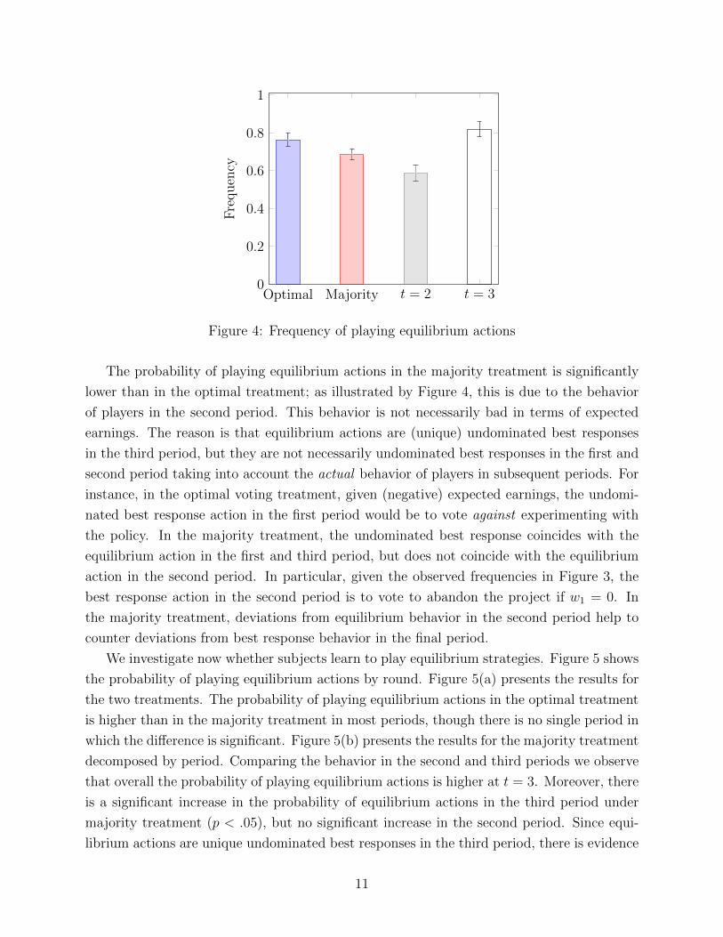
We investigate now whether subjects learn to play equilibrium strategies. Figure 5 shows

the probability of playing equilibrium actions by round. Figure 5(a) presents the results for

the two treatments. The probability of playing equilibrium actions in the optimal treatment

is higher than in the majority treatment in most periods, though there is no single period in

which the di↵erence is significant. Figure 5(b) presents the results for the majority treatment

decomposed by period. Comparing the behavior in the second and third periods we observe

that overall the probability of playing equilibrium actions is higher at t = 3. Moreover, there

is a significant increase in the probability of equilibrium actions in the third period under

majority treatment (p < .05), but no significant increase in the second period. Since equi-

librium actions are unique undominated best responses in the third period, there is evidence

11

2 4 6 8 10 12 14

0

0.2

0.4

0.6

0.8

1

Round

Frequ

ency

MajorityOptimal

2 4 6 8 10 12 14

0

0.2

0.4

0.6

0.8

1

Round

Frequ

ency

t = 2t = 3

(a) By treatment (b) By period

Figure 5: Frequency of playing equilibrium actions over time

of learning. The situation in the second period is more involved; if learning equilibrium

actions in the third period were closer to completely successful, it would make sense to play

equilibrium actions in the third period.

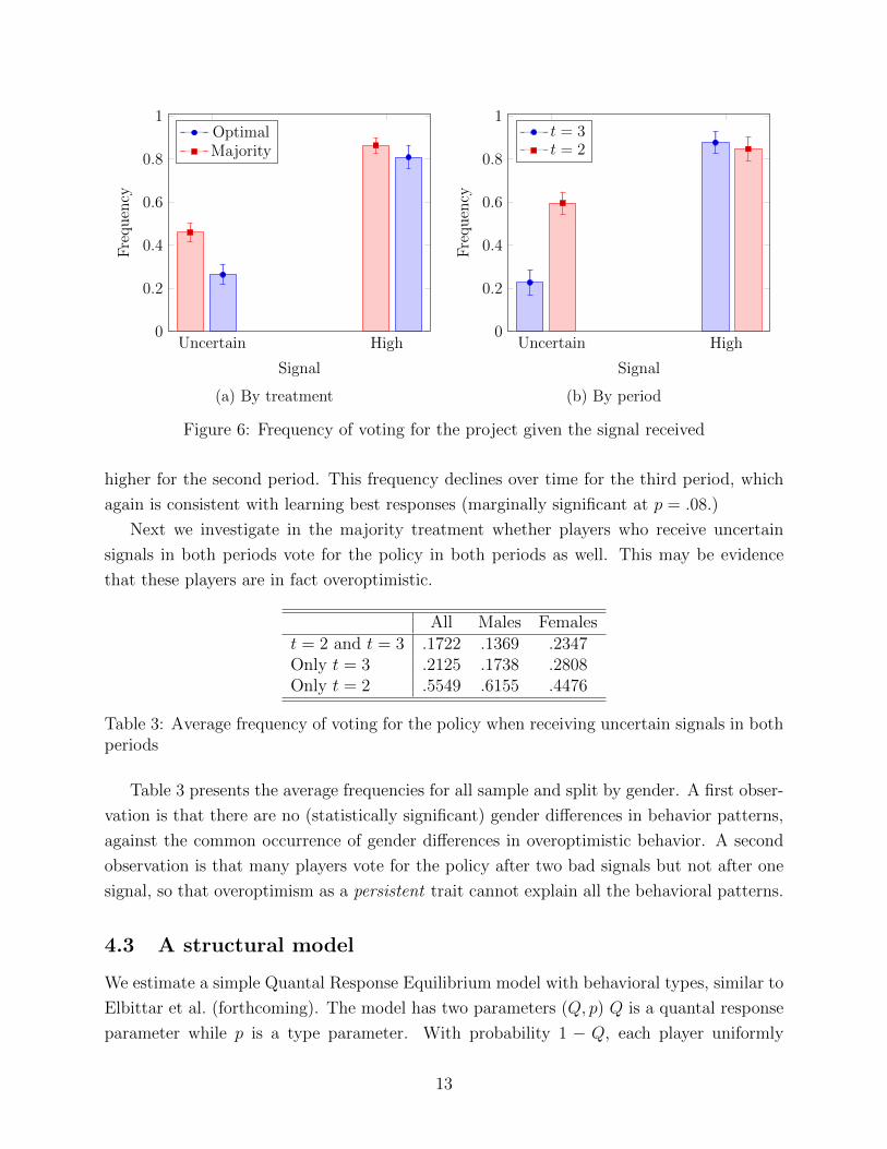
Figure 6(a) shows the frequency of voting for the policy conditional on the signal received

for both treatments. Note that voting for the policy after a high signal is the unique undom-

inated best response. There is no di↵erence in voting for the policy in this case. Note also

that voting for the policy after uncertain signals in the third period reduces the expected

earnings of the player; it can be attributed to overoptimistic expectations regarding the rev-

enue of the project for the player. For the optimal treatment, in particular, the frequency of

voting for the policy (around 25%) is evidence in favor of a bias for overoptimism. For the

majority treatment the situation is more involved; voting for the project in the third period

is evidence in support of overoptimism, but voting for the project in the second period may

or may not be a best response.

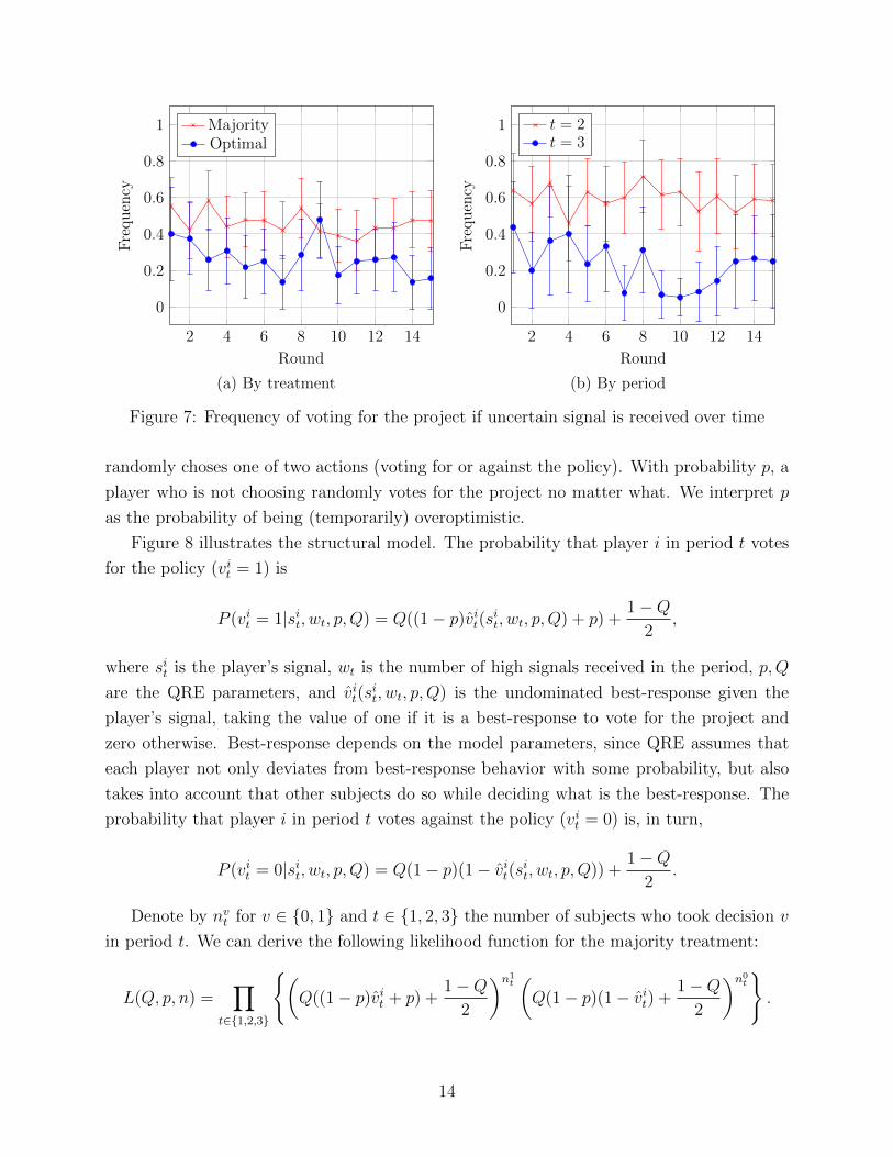
We investigate now whether overoptimistic behavior is persistent feature along the repe-

titions of the game. Figure 7 shows the frequency of voting for the policy after receiving an

uncertain signal by round. Figure 7(a) shows the frequency for di↵erent treatments. This

frequency declines over time for the optimal treatment, which is consistent with learning

best responses (marginally significant at p = .07). It remains relatively high for the majority

treatment, where it may reflect the fact that voting for the policy in the second period after

an uncertain signal may be a best response (and in fact it is the equilibrium action if no one

else obtains high signals).

Figure 7(b) shows the frequency of voting for the policy after an uncertain signal for t = 2

and t = 3 in the majority treatment over di↵erent rounds. The frequency is systematically

12

Uncertain High0

0.2

0.4

0.6

0.8

1

Signal

Frequ

ency

OptimalMajority

Uncertain High0

0.2

0.4

0.6

0.8

1

Signal

Frequ

ency

t = 3t = 2

(a) By treatment (b) By period

Figure 6: Frequency of voting for the project given the signal received

higher for the second period. This frequency declines over time for the third period, which

again is consistent with learning best responses (marginally significant at p = .08.)

Next we investigate in the majority treatment whether players who receive uncertain

signals in both periods vote for the policy in both periods as well. This may be evidence

that these players are in fact overoptimistic.

All Males Femalest = 2 and t = 3 .1722 .1369 .2347Only t = 3 .2125 .1738 .2808Only t = 2 .5549 .6155 .4476

Table 3: Average frequency of voting for the policy when receiving uncertain signals in bothperiods

Table 3 presents the average frequencies for all sample and split by gender. A first obser-

vation is that there are no (statistically significant) gender di↵erences in behavior patterns,

against the common occurrence of gender di↵erences in overoptimistic behavior. A second

observation is that many players vote for the policy after two bad signals but not after one

signal, so that overoptimism as a persistent trait cannot explain all the behavioral patterns.

4.3 A structural model

We estimate a simple Quantal Response Equilibrium model with behavioral types, similar to

Elbittar et al. (forthcoming). The model has two parameters (Q, p) Q is a quantal response

parameter while p is a type parameter. With probability 1 � Q, each player uniformly

13

2 4 6 8 10 12 14

0

0.2

0.4

0.6

0.8

1

Round

Frequ

ency

MajorityOptimal

2 4 6 8 10 12 14

0

0.2

0.4

0.6

0.8

1

Round

Frequ

ency

t = 2t = 3

(a) By treatment (b) By period

Figure 7: Frequency of voting for the project if uncertain signal is received over time

randomly choses one of two actions (voting for or against the policy). With probability p, a

player who is not choosing randomly votes for the project no matter what. We interpret p

as the probability of being (temporarily) overoptimistic.

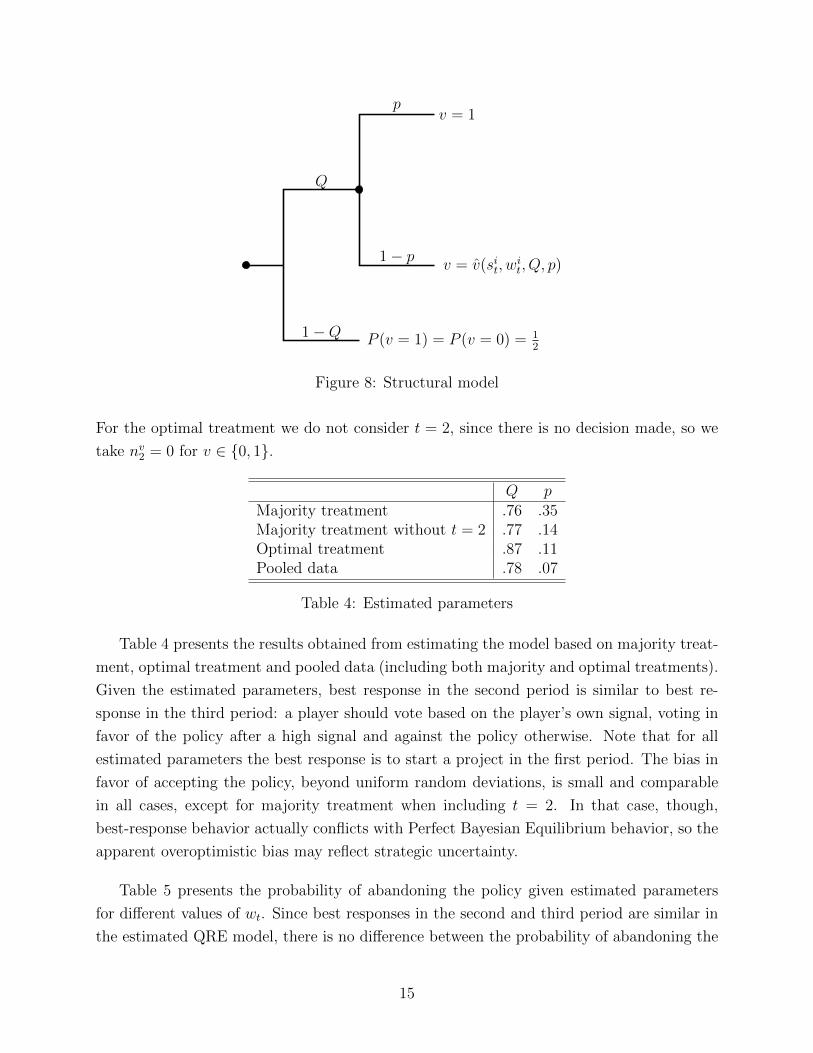
Figure 8 illustrates the structural model. The probability that player i in period t votes

for the policy (vit = 1) is

P (vit = 1|sit, wt, p, Q) = Q((1� p)vit(sit, wt, p, Q) + p) +

1�Q

2,

where sit is the player’s signal, wt is the number of high signals received in the period, p,Q

are the QRE parameters, and vit(sit, wt, p, Q) is the undominated best-response given the

player’s signal, taking the value of one if it is a best-response to vote for the project and

zero otherwise. Best-response depends on the model parameters, since QRE assumes that

each player not only deviates from best-response behavior with some probability, but also

takes into account that other subjects do so while deciding what is the best-response. The

probability that player i in period t votes against the policy (vit = 0) is, in turn,

P (vit = 0|sit, wt, p, Q) = Q(1� p)(1� vit(sit, wt, p, Q)) +

1�Q

2.

Denote by nvt for v 2 {0, 1} and t 2 {1, 2, 3} the number of subjects who took decision v

in period t. We can derive the following likelihood function for the majority treatment:

L(Q, p, n) =Y

t2{1,2,3}

(

✓

Q((1� p)vit + p) +1�Q

2

◆n1

t✓

Q(1� p)(1� vit) +1�Q

2

◆n0

t

)

.

14

Q

1�Q

p

1� p

P (v = 1) = P (v = 0) = 12

v = 1

v = v(sit, wit, Q, p)

Figure 8: Structural model

For the optimal treatment we do not consider t = 2, since there is no decision made, so we

take nv2 = 0 for v 2 {0, 1}.

Q pMajority treatment .76 .35Majority treatment without t = 2 .77 .14Optimal treatment .87 .11Pooled data .78 .07

Table 4: Estimated parameters

Table 4 presents the results obtained from estimating the model based on majority treat-

ment, optimal treatment and pooled data (including both majority and optimal treatments).

Given the estimated parameters, best response in the second period is similar to best re-

sponse in the third period: a player should vote based on the player’s own signal, voting in

favor of the policy after a high signal and against the policy otherwise. Note that for all

estimated parameters the best response is to start a project in the first period. The bias in

favor of accepting the policy, beyond uniform random deviations, is small and comparable

in all cases, except for majority treatment when including t = 2. In that case, though,

best-response behavior actually conflicts with Perfect Bayesian Equilibrium behavior, so the

apparent overoptimistic bias may reflect strategic uncertainty.

Table 5 presents the probability of abandoning the policy given estimated parameters

for di↵erent values of wt. Since best responses in the second and third period are similar in

the estimated QRE model, there is no di↵erence between the probability of abandoning the

15

wt = 0 wt = 1 wt = 2 wt = 3Majority treatment (Q = .76, p = .35) .67 .43 .14 .04Majority without t = 2 (Q = .77, p = .14) .87 .64 .17 .04Optimal treatment (Q = .87, p = .11) .93 .71 .11 .01Pooled data (Q = .78, p = .07) .93 .73 .18 .03

Table 5: Probabilities of stopping the policy conditional on wt high signals

project in the second and third periods. The estimations are relatively close the observed

frequencies, except for majority treatment when including t = 2.

Finally, we attempt to classify subjects in persistent types, best-responder or overopti-

mistic, using likelihood ratios. For the majority treatment, every subject participated in 15

repetitions of the game and made at least once decision, so that for every subject we have

between 15 and 45 observations. Similarly, for the optimal treatment, we have between 15

and 30 decisions for every subject.

Persistent best responder and overoptimistic types have di↵erent likelihood functions, and

we compare the odds of them. For all estimated decision making errors the best response

is to start a project and to vote further according to the signal player received. Hence, if

we denote by kvt the amount of times then player voted v 2 {0, 1} in period t, we can write

down the following likelihood ratio:

�(Q, k) =

�

Q+ 1�Q2

�k11

�

1�Q2

�k01

Q

t2{2,3}

n

�

Qsit +1�Q2

�k1t�

Q(1� sit) +1�Q2

�k0to

Q

t2{1,2,3}

n

�

Q+ 1�Q2

�k1t�

1�Q2

�k0to .

The numerator corresponds to the likelihood that the player is a best-responder given Q,

while the denominator corresponds to the likelihood that the player is overoptimistic given

Q. If �(Q, k) > 20 we classify a player as best responder, if �(Q, k) < 120 we classify player

as overoptimistic, otherwise the player is unclassified. One can interpret 20 : 1 odds, for

descriptive purposes, as indicating with 95% confidence that the subject is correctly classified

by the estimated model.

Majority Majority without t = 2 Optimal Pooledbest responders .50 .97 .79 .62unclassified .28 .03 .21 .25overoptimistic .22 .00 .00 .13

Table 6: Classification of subjects

Table 6 presents the fraction of subject classified by treatment and with pooled data. For

16

every column we use the parameter Q estimated from the sample (see Table 4). Except for

majority treatment when including t = 2, subjects are either classified as best-responders or

left unclassified, with few exceptions. This is further evidence against persistent overopti-

mistic types.

Note that the observed over experimentation cannot be explained by risk aversion. The

more risk-averse players are, the more they would under experiment. We conclude that the

observed behavior may be due to over optimism, but not to persistent types.

5 Final remarks

We construct a simple three-period political economy model of experimentation. In the

model, after a policy is adopted, individual voters may obtain or not conclusive signals that

they will be winners from the policy. We show that majority rule may have a bias toward

under experimentation, capturing a strategic consequence of collective experimentation first

identified by Strulovici (2010), and describe an optimal voting rule. The optimal voting

rule either requires unanimity for abandoning the policy in intermediate stages, or simply

eschews voting in intermediate stages.

We implement the model in the lab with three-player groups. Against equilibrium pre-

dictions, we find over experimentation in the lab when there is little evidence in support of

adopting the policy under both majority voting and the (theoretically) optimal voting rule.

This causes majority voting to outperform the optimal voting rule: allowing voters to vote

at intermediate stages about the policy allows them to reduce the probability that the policy

is adopted for good by mistakes made in the final stage.

We interpret mistakes in favor of adopting the policy for good in the final stage as a

consequence of over optimism. We find very little evidence in support of persistent overopti-

mism for individual subjects in the lab implementation. Some of the results may reflect the

complexity of the strategic calculus for lab participants when best response behavior given

the actual behavior of other players conflict with equilibrium predictions. Also, the impact

of individual mistakes on group decision may be lower in larger groups. Finding ways to pro-

vide subjects with more feedback about the behavior of other subjects without stretching the

design beyond what is reasonable, and using larger groups, seem avenues worth exploring.

Appendix A: Proofs

Lemma 1. The utilitarian social planner and majority voting outcomes coincide in the third

period if and only if1

2<

h� s

s� r< 2.

17

Proof. Since by assumption r = p2h + (1� p2)l < s, only players who received high signals

would vote to adopt the policy in the last period. Therefore, under the majority rule the

outcome would be to implement the policy if there were at least two good signals and abandon

otherwise. The utilitarian social planner, instead, would make a decision based on the total

welfare amount. The total utility from abandoning the policy in favor of safe alternative is

3s, the payo↵ from implementing the risky alternative after two high signals is 2h + r, and

the payo↵ from implementing the project after receiving only one high signal is h+2r. The

condition in the lemma guarantees that the social planer’s actions to coincide with majority

voting.

Lemma 2. If w1 = 1, voters will abandon the policy in the second period if and only if

h� s

s� r< 1� p1q.

Proof. Suppose w1 = 1, and consider the players who did not receive a high signal. Their

expected payo↵ can be decomposed in the following three cases:

(i) The player receives a high signal in the next period. Then the player’s payo↵ is h

for sure, since there are at least two agents with high signals and the project will be

implemented.

(ii) The player does not receive a high signal but the other player does. Then the player’s

payo↵ is r since there are two players receiving high signals and the policy will be

implemented.

(iii) None of the two players receive high signals in the next period. Then, the player’s

payo↵ is s since the project will be abandoned.

The expected payo↵ from voting for continue experimenting is then:

E⇡(Continue) = p1qh+ p1q(1� p1q)r + (1� p1q)2s.

The alternative is to abandon the project and receive the safe payo↵. Hence, the net gain of

adopting the policy is

E⇡(Continue)� s = p1q ((h� s) + (1� p1q)(r � s)) ,

which is negative if and only if (h� s)/(s� r) < 1� p1q. Hence, under the condition of the

lemma, the two players who did not receive the high signal prefer to abandon the policy in

the second period.

18

Lemma 3. If w1 = 0, voters will continue the policy in the second period if and only if

h� s

s� r� 1� p1q

2� p1q.

Proof. Suppose w1 = 0 and consider any of the three players. If the policy continues, it will

be adopted in the final period in two cases:

(i) The player obtains a high signal and at least another player does. The probability of

this event is p1q(2p1q(1� p1q) + (p1q)2) = (p1q)2(2� p1q), and in this case the player

obtains a payo↵ of h.

(ii) The player does not obtain a high signal but the other two players do. The probability

of this event is (1� p1q)(p1q)2, and in this case the player obtains a payo↵ of r.

In the remainder event the policy is not adopted in the final period and the player obtains

a payo↵ of s. Hence, the net gain of adopting the policy is:

E⇡(Continue)� s = (p1q)2 ((h� s)(2� p1q) + (r � s)(1� p1q)) ,

which is negative if and only if (h � s)/(s � r) < (1 � p1q)/(2 � p1q). Hence, the player

prefers to abandon the policy in the second period if and only if this inequality holds.

Lemma 4. If1� p1q

2� p1q h� s

s� r< 1� p1q,

voters will start experimenting with the policy in the first period.

Proof. First, let us find the probability of receiving a high payo↵ for sure in the last period

if the reform is started. There are two possible cases: either the player receives a high signal

at t = 1 (which occurs with probability p0q) or the player does not receive a high signal

at t = 1 but receives a high signal at t = 2 (which occurs with probability (1 � p0q)p1q).

The following table summarizes the probabilities of implementing the policy conditional on

possible events in these two cases.

High signal received at t w1 w2 Probability1 2 2 or 3 2p0q(1� p0q)1 3 3 (p0q)2

2 0 2 (1� p0q)22(p1q)(1� p1q)2 0 3 (1� p0q)2(p1q)2

2 2 3 (p0q)2

19

In the table we use the fact that the project is stopped if there is only one high signal

received in the first period, as implied by Lemma 2.

Now, let us calculate the probability of receiving a payo↵ of r if the reform is started. In

this case player cannot receive a high signal, which happens with probability (1�p0q)(1�p1q).

Then, the project is implemented if either both other players receive high signals at t = 2

(which happens with probability (p0q)2) or neither of them receive a high signal at t = 2

and both receive high signals at t = 3 (which happens with probability (1� p0q)2(p1q)2).

Then, the expected net gain of adopting the policy in the first period is:

E⇡(Continue)� s = (h� s)⇥

p0q�

2p0q(1� p0q) + (p0q)2�

+ (1� p0q)p1q�

(1� p0q)2(2(p1q)(1� p1q) + (p1q)

2) + (p0q)2�⇤

+(s� r)(1� p0q)(1� p1q)⇥

(p0q)2 + (1� p0q)

2(p1q)2⇤

.

Substituting and simplifying,

E⇡(Continue)� s = (h� s)(p0q)2⇥

2� p0q2 + (1� q)2(2� 3p0q + p0q

2)⇤

+(s� r)(p0q)2(1� 2p0q + p0q

2)(1 + (1� q)2).

Thus, every player prefers to adopt the policy in the first period if

h� s

s� r� (p0q)2(1� 2p0q + p0q2)(1 + (1� q)2)

(p0q)2 [2� p0q2 + (1� q)2(2� 3p0q + p0q2)], (1)

or equivalently

h� s

s� r� (1� p0q)(1� p1q)(1 + (1� q)2)

1 + (1� p0q)[(1� q)2 + (1� p1q)(1 + (1� q)2)].

We can rewrite this inequality as

1 +1

1� p1q+

p0q

(1� p0q)(1� p1q)(1 + (1� q)2)� s� r

h� s,

while we can rewrite the condition for Lemma 3 as

1 +1

1� p1q� s� r

h� s,

which is more demanding.

Lemma 5. Suppose1

2 h� s

s� r< 1� p1q.

20

Then, the voting rule that requires simple majority to start the project in the first period

and to adopt if for good in the third period, but specifies no voting in the second period,

implements the utilitarian social planner outcomes.

Proof. Since the condition of Lemma 1 is satisfied, simple majority outcomes in the last

period coincide with the utilitarian outcomes. It remains to be shown that voters adopt the

policy under simple majority in the first period when they know that there will be no voting

until the final period.

The calculation is similar to the one in the proof of Lemma 4. To the events leading to

receiving a high payo↵ for sure in the last period, we have to add the events in which only

one high signal is received in the first period:

High signal received at t w1 w2 Probability1 1 2 (1� p0q)22p1q(1� p1q)1 1 3 (1� p0q)2(p1q)2

2 1 2 or 3 2p0q(1� p0q)

Thus, respect to the calculation in the proof of Lemma 4, equation 1, the probability of

receiving a payo↵ of h in rather than s in the third period increases in

p0q(1� p0q)2�

2p1q(1� p1q) + (p1q)2�

+ (1� p0q)p1q2p0q(1� p0q),

or equivalently,

p0q(1� p0q)2�

2p1q(1� p1q) + (p1q)2 + 2p1q

�

⌘ A.

Similarly, to the events leading to receiving a expected payo↵ of r in the last period, we have

to add the event in which only one high signal is received by other players in the first period,

with the other player receiving a high signal in the second period, which has probability

2(p0q)(1�p0q)p1q. Thus, respect to the calculation in the proof of Lemma 4, the probability

of receiving a payo↵ of r in rather than s in the third period increases in

(1� p0q)(1� p1q)2p0q(1� p0q)p1q,

or equivalently,

p0q(1� p0q)2(1� p1q)(2p1q) ⌘ B.

Following the steps of the proof of Lemma 4, the condition for players to vote for adopting

the policy in the first period is then

h� s

s� r� (p0q)2(1� 2p0q + p0q2)(1 + (1� q)2) + B

(p0q)2 [2� p0q2 + (1� q)2(2� 3p0q + p0q2)] + A.

21

It is easy to check that A > B, so if inequality 1 is satisfied, the condition above is satisfied

as well.

References

James Albrech, Axel Anderson, and Susan Vroman. Search by committee. Journal of

Economic Theory, 145(1386-1407), 2010.

James Buchanan and Gordon Tullock. The Calculus of Consent. The University of Michigan

Press, 1962.

Steven Callander and Patrick Hummel. Preemptive policy experimentation. Econometrica,

82:1509–1528, 2014.

Jimmy Chan, Alessandro Lizzeri, Wing Suen, and Leeat Yariv. Deliberating collective deci-

sions. Review of Economic Studies, 2015.

Daniel L Chen, Martin Schonger, and Chris Wickens. otree—an open-source platform for

laboratory, online, and field experiments. Journal of Behavioral and Experimental Finance,

9:88–97, 2016.

Alexander Elbittar, Andrei Gomberg, Cesar Martinelli, and Thomas R Palfrey. Ignorance

and bias in collective decisions. Journal of Economic Behavior & Organization, forthcom-

ing.

Raquel Fernandez and Dani Rodrik. Resistance to reform: Status quo bias in the presence

of individual-specific uncertainty. American Economic Review, pages 1146–1155, 1991.

Daria Khromenkova. Collective experimentation with breakdowns and breakthroughs. Uni-

versity of Mannheim (unpublished), 2017.

Richard D McKelvey and Thomas R Palfrey. Quantal response equilibria for normal form

games. Games and Economic Behavior, 10(1):6–38, 1995.

Richard D McKelvey and Thomas R Palfrey. Quantal response equilibria for extensive form

games. Experimental Economics, 1(1):9–41, 1998.

Matthias Messner and Mattias K Polborn. The option to wait in collective decisions and

optimal majority rules. Journal of Public Economics, 96(5):524–540, 2012.

Benny Moldovanu and Xianwen Shi. Specialization and partisanship in committee search.

Theoretical Economics, 8(3):751–774, 2013.

22

Bruno Strulovici. Learning while voting: Determinants of collective experimentation. Econo-

metrica, 78(3):933–971, 2010.

23

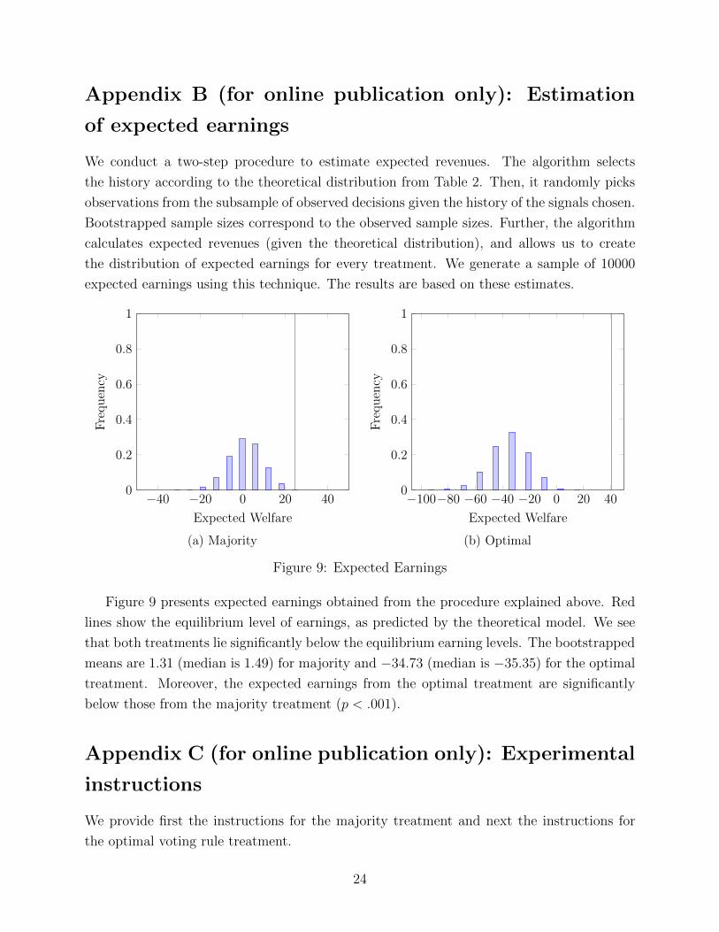
Appendix B (for online publication only): Estimation

of expected earnings

We conduct a two-step procedure to estimate expected revenues. The algorithm selects

the history according to the theoretical distribution from Table 2. Then, it randomly picks

observations from the subsample of observed decisions given the history of the signals chosen.

Bootstrapped sample sizes correspond to the observed sample sizes. Further, the algorithm

calculates expected revenues (given the theoretical distribution), and allows us to create

the distribution of expected earnings for every treatment. We generate a sample of 10000

expected earnings using this technique. The results are based on these estimates.

�40 �20 0 20 400

0.2

0.4

0.6

0.8

1

Expected Welfare

Frequ

ency

�100�80 �60 �40 �20 0 20 400

0.2

0.4

0.6

0.8

1

Expected Welfare

Frequ

ency

(a) Majority (b) Optimal

Figure 9: Expected Earnings

Figure 9 presents expected earnings obtained from the procedure explained above. Red

lines show the equilibrium level of earnings, as predicted by the theoretical model. We see

that both treatments lie significantly below the equilibrium earning levels. The bootstrapped

means are 1.31 (median is 1.49) for majority and �34.73 (median is �35.35) for the optimal

treatment. Moreover, the expected earnings from the optimal treatment are significantly

below those from the majority treatment (p < .001).

Appendix C (for online publication only): Experimental

instructions

We provide first the instructions for the majority treatment and next the instructions for

the optimal voting rule treatment.

24

Instructions

Welcome to our experiment! You have earned $5 by showing up on time. If you read and follow the instructions below carefully, you have the potential to earn up to $35. In the experiment you will earn Experimental Dollars (E$s) which will be converted into cash at the end of the experiment. For every 20 E$ you have at the end of the experiment you will be paid 1 US Dollar. You will NOT be told the names of those in your group and they will NOT be told your name. All participants have identical instructions. NO communication with other participants is allowed during this experiment. Please switch off your cell phones. If you have any questions please raise your hand, and the experimenter will assist you individually.

Decision Task

There are 15 rounds in this experiment. At the end of this experiment, only 1 round will be randomly selected to determine your final payment. Every round has equal chance of being chosen as the payoff round, therefore it is in your best interest to treat each round as if it is the one that determines your payment. At the beginning of each round, three players will compose a group, and each of you will get a Player ID (for example, Player 1, Player 2 or Player 3). The Player ID may vary from round to round. For each round, you will be randomly placed in a new group.

There is one project at each round (different project at different round). You and the other two group members jointly decide whether or not to implement a project. If a project is implemented, each of you has 50% chance to receive a high payoff: E$500, and a 50% chance to receive a low payoff: E$50. Whether each of you receive a high payoff or low payoff is independently and randomly determined at the beginning of each round. If the project is NOT implemented, each of you will receive E$350 for sure.

There are three stages for each round. At each stage, each of you will choose an action. The majority action of the group (i.e. at least two players) will be the action realized.

At Stage 1, each of you can choose INITIATE or STOP the project right away. If the majority of you choose to STOP, the project is NOT implemented and this round ends. If the majority of you choose to INITIATE the project, each of you will get a signal regarding whether you can receive high payoff if the project is implemented. The signal works in the following way:

The signal is programmed to be either “High payoff for sure” or “Uncertain.” If you are a player who will receive high payoff if the project is implemented, there is 50% chance for you to receive a signal that says “High payoff for sure”, and another 50% to receive a signal that says “Uncertain”. If you are a player who will receive the low payoff if the project is implemented, you will always receive a signal that says “Uncertain.” In other words, if you get a “High payoff for sure” signal, you will keep receiving the same signal in the following

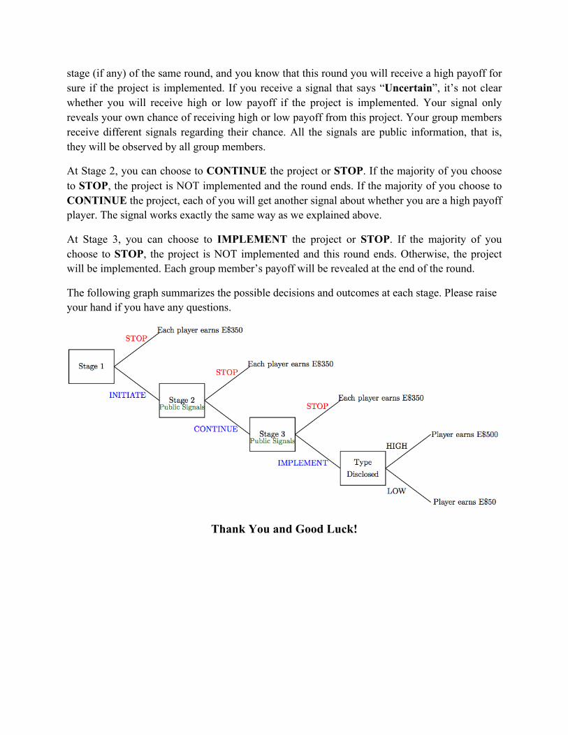
stage (if any) of the same round, and you know that this round you will receive a high payoff for sure if the project is implemented. If you receive a signal that says “Uncertain”, it’s not clear whether you will receive high or low payoff if the project is implemented. Your signal only reveals your own chance of receiving high or low payoff from this project. Your group members receive different signals regarding their chance. All the signals are public information, that is, they will be observed by all group members.

At Stage 2, you can choose to CONTINUE the project or STOP. If the majority of you choose to STOP, the project is NOT implemented and the round ends. If the majority of you choose to CONTINUE the project, each of you will get another signal about whether you are a high payoff player. The signal works exactly the same way as we explained above.

At Stage 3, you can choose to IMPLEMENT the project or STOP. If the majority of you choose to STOP, the project is NOT implemented and this round ends. Otherwise, the project will be implemented. Each group member’s payoff will be revealed at the end of the round.

The following graph summarizes the possible decisions and outcomes at each stage. Please raise your hand if you have any questions.

Thank You and Good Luck!

Instructions

Welcome to our experiment! You have earned $5 by showing up on time. If you read and follow the instructions below carefully, you have the potential to earn up to $35. In the experiment you will earn Experimental Dollars (E$s) which will be converted into cash at the end of the experiment. For every 20 E$ you have at the end of the experiment you will be paid 1 US Dollar. You will NOT be told the names of those in your group and they will NOT be told your name. All participants have identical instructions. NO communication with other participants is allowed during this experiment. Please switch off your cell phones. If you have any questions please raise your hand, and the experimenter will assist you.

Decision Task

There are 30 rounds in this experiment. At the end of this experiment, only 1 round will be randomly selected to determine your final payment. Every round has equal chance of being chosen as the payoff round, therefore it is in your best interest to treat each round as if it is the one that determines your payment. At the beginning of each round, three players will compose a group, and each of you will get a Player ID (for example, Player 1, Player 2 or Player 3). The Player ID may vary from round to round. For each round, you will be randomly placed in a new group.

There is one project at each round (different project at different round). You and the other two group members jointly decide whether or not to implement a project. If a project is implemented, each of you has 50% chance to receive a high payoff: E$500, and a 50% chance to receive a low payoff: E$50. Whether each of you receive a high payoff or low payoff is independently and randomly determined at the beginning of each round. If the project is NOT implemented, each of you will receive E$350 for sure.

There are three stages for each round. At each stage, each of you will choose an action. The majority action of the group (i.e. at least two players) will be the action realized.

At Stage 1, each of you can choose INITIATE or STOP the project right away. If the majority of you choose to STOP, the project is NOT implemented and this round ends. If the majority of you choose to INITIATE the project, each of you will get a signal regarding whether you can receive high payoff if the project is implemented. The signal works in the following way:

The signal is programmed to be either “High payoff for sure” or “Uncertain.” If you are a player who will receive high payoff if the project is implemented, there is 50% chance for you to receive a signal that says “High payoff for sure”, and another 50% to receive a signal that says “Uncertain”. If you are a player who will receive the low payoff if the project is implemented, you will always receive a signal that says “Uncertain.” In other words, if you get a “High payoff for sure” signal, you will keep receiving the same signal in the following

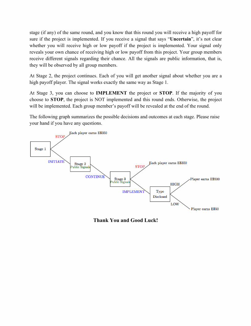
stage (if any) of the same round, and you know that this round you will receive a high payoff for sure if the project is implemented. If you receive a signal that says “Uncertain”, it’s not clear whether you will receive high or low payoff if the project is implemented. Your signal only reveals your own chance of receiving high or low payoff from this project. Your group members receive different signals regarding their chance. All the signals are public information, that is, they will be observed by all group members.

At Stage 2, the project continues. Each of you will get another signal about whether you are a high payoff player. The signal works exactly the same way as Stage 1.

At Stage 3, you can choose to IMPLEMENT the project or STOP. If the majority of you choose to STOP, the project is NOT implemented and this round ends. Otherwise, the project will be implemented. Each group member’s payoff will be revealed at the end of the round.

The following graph summarizes the possible decisions and outcomes at each stage. Please raise your hand if you have any questions.

Thank You and Good Luck!