*QuadTech

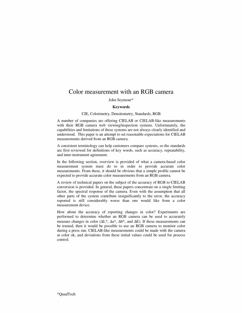
Color measurement with an RGB camera

John Seymour*

Keywords

CIE, Colorimetry, Densitometry, Standards, RGB

A number of companies are offering CIELAB or CIELAB-like measurements

with their RGB camera web viewing/inspection systems. Unfortunately, the

capabilities and limitations of these systems are not always clearly identified and

understood. This paper is an attempt to set reasonable expectations for CIELAB

measurements derived from an RGB camera.

A consistent terminology can help customers compare systems, so the standards

are first reviewed for definitions of key words, such as accuracy, repeatability,

and inter-instrument agreement.

In the following section, overview is provided of what a camera-based color

measurement system must do to in order to provide accurate color

measurements. From these, it should be obvious that a simple profile cannot be

expected to provide accurate color measurements from an RGB camera.

A review of technical papers on the subject of the accuracy of RGB to CIELAB

conversion is provided. In general, these papers concentrate on a single limiting

factor, the spectral response of the camera. Even with the assumption that all

other parts of the system contribute insignificantly to the error, the accuracy

reported is still considerably worse than one would like from a color measurement device.

How about the accuracy of reporting changes in color? Experiments are

performed to determine whether an RGB camera can be used to accurately

measure changes in color (∆L*, ∆a*, ∆b*, and ∆E). If these measurements can be trusted, then it would be possible to use an RGB camera to monitor color

during a press run. CIELAB-like measurements could be made with the camera

at color ok, and deviations from these initial values could be used for process

control.

How Good Is Good Enough?

Important definitions

When printers are considering adding a color reporting option to their web

inspection system, they would like to know how much they can rely on the

measurements. Beyond just the desire to make informed decisions between

vendors, the quality of the numbers determines what they can be used for. The

vendors have responded with a confusing array of specifications. This unfortunately makes it difficult to compare one set of vendor claims against

another.

The following are definitions for key words that appear in specifications. The

definitions, where possible, are based on standards, particularly ASTM (2002).

Precision This term is not defined in any standard on colorimetry. The word is

used in the standards, however, in two ways. In some cases, it is used to mean a

general sense of the quality of a set of measurements. In other cases the words

refers to the number of digits in the reporting of a measurement. The former is

an imprecise way to specify an instrument, and the latter is irrelevant, provided

there are enough digits reported. This word should not be to specify an

instrument.

Resolution This term is also not defined in any standard on colorimetry. The

scientific definition is given in Van Nostrand (1968): “A term used in a number

of specific cases in science to denote the process of separating closely related

forms or identities or the degree that can be discriminated.” Thus, subjecting a

colorimeter to the Farnsworth-Munsell 100 hue test – testing to see if the

instrument can reliably resolve the differences between tiny differences in color

– is a test of the colorimeter’s resolution.

Repeatability “The ISO VIM (ISO 1993) defines repeatability as a measure of

the random error of a reading and assumes that the sample standard deviation is

an estimate of repeatability. Repeatability is further defined as the standard

deviation of a set of measurements taken over a specified time period by a single

operator, on a single instrument with a single specimen.” (ASTM 2002). The repeatability of a colorimeter is determined by making multiple measurements

of a single sample in a short period of time, without moving the instrument.

Note that the average of multiple measurements generally has a smaller (that is,

better) repeatability than a single measurement, so repeatability can actually be

improved by taking multiple measurements.

Reproducibility “The ISO VIM (ISO 1993) defines reproducibility as a type of

repeatability in which either the time frame is very long, in which the operator

changes, the instrument changes, or the measurement conditions change.”

(ASTM 2002)

The repeatability and reproducibility of an instrument are similar and are both

useful. The reproducibility of an instrument is more important under normal use.

However, the repeatability is useful in assessing the instrument itself and its

contribution to the overall variability.

This distinction is useful for an online measurement tool where measurement

error includes the sheet to sheet variation of the printing process as well as the repeatability of the instrument. If the repeatability of the instrument is less than,

say, half the sheet to sheet variation, then the instrument may be deemed

acceptable.

Inter-instrument agreement “Inter-instrument agreement … describes the

reproducibility between two or more instruments, of identical design. The ISO

has no definition or description of such a concept. This is because in most test

results, a method or instrument dependent bias can be assessed.” (ASTM 2002)

The last sentence states that it is usually possible to provide a correction

between two units. I would discourage this. The correction is generally sample

dependent.

Inter-model agreement “Inter-model agreement … describes the reproducibility between two or more instruments of different design.” (ASTM 2002)

Inter-instrument agreement is the most commonly reported spec. From the

manufacturer’s standpoint, this is the most sensible spec to report, since it only

involves their own instruments.

Customers of online color measurement systems are most interested in the spec

for inter-model agreement. It is important that a measurement on the web agrees

with measurements taken offline with a handheld spectrophotometer.

Unfortunately, specifying inter-model agreement is problematic for a vendor,

since it depends not only on their own instrument, but an instrument from

another vendor. Just as importantly, inter-model agreement depends on the

proper care and upkeep of the both instruments.

Accuracy “ISO defines accuracy as the conformance of a series of readings to the accepted or true value.” (ASTM 2002) For colorimetry, the “accepted or true

value” means “measurements taken at a standards lab.” Thus, accuracy means

the inter-model agreement with a standards lab.

Generally, accuracy is established through the BCRA tiles. These are a set of

twelve ceramic tiles originally developed by the British Ceramic Research

Association. These tiles are measured by a standards lab such as NIST, and then

measured with the colorimeter to verify accuracy.

This verification establishes that the colorimeter is capable of accurately

measuring BCRA tiles. It can be expected that, the greater a sample differs from

the characteristics of the BCRA tiles, the greater the opportunity for differences

in readings. An ideal reference sample would be actual print. This is

unfortunately an unsuitable reference since it is prone to aging, physical

damage, and is not easily cleaned.

It is natural for a customer to want to have their instrument report most

accurately what the true color of a sample is. But, unlike a volt or an inch, the

color perceived depends upon at least two factors external to the sample. First,

the measurement of a sample depends upon the angles of illumination and of viewing. Second, the spectral characteristic of the lighting is important. Samples

that match under incandescent light may not match under sunlight or under

fluorescent light.

This second issue has become more of a concern of late. Fluorescent brightening

agents are becoming more and more common in paper, so the amount of UV

light directed on the sample has a large effect on the color seen or measured.

For these reasons, “accuracy” is kind of a slippery term, especially in the

printing industry.

What are the requirements?

ISO 12647-2 (ISO 2004) is a standard that covers the entire web offset print

process. There are three colorimetric requirements in this standard.

The first requirement is that solid process colors on a proof must be within 5 ∆E

of specific CIELAB numbers in the document. This imposes an accuracy

requirement for the colorimeter used on incoming proofs. This requirement does

not apply to an online system, provided that the online system is not used to

measure the proof.

The second colorimetric requirement in ISO 12647-2 (ISO 2004) does apply to

an online colorimeter. The process color solids on the color OK sheet must be

within 5 ∆E of those on the proof sheet. Presumably, two different instruments would be used to measure the proof and the color OK sheet, so this imposes an

intra-model agreement specification between the press side and online

colorimeters. The larger the discrepancy between the two instruments, the more

likely it is that good product will be rejected and bad product accepted.

How much of a discrepancy between instruments is acceptable? If the overall measurement error exceeds 30% of the tolerance window, then the measurement

device is considered unacceptable for determining whether product is in

tolerance. An error of 10% or less is considered acceptable. In between, the

device is considered marginally acceptable.

At first, one might feel that the range of acceptability is 5 ∆E. However, the

maximum range for L* would be the target value, plus or minus 5 ∆E. The total

tolerance range is thus 10 ∆E. Thus, the accuracy of the colorimeter used to

assess an OK sheet must be no more than 3 ∆E, but ideally, should be 1 ∆E.

The third colorimetric requirement in ISO 12647-2 (ISO 2004) specifies how

well color is maintained during the run. It stipulates that 68% of the process

color solids printed during the run must be within 4 ∆E, and 68% should be

within 2 ∆E . What sort of specification does this imply for our colorimeter? It’s not exactly a reproducibility spec, since reproducibility assumes that the sample

is not changing (just everything else). The most reasonable way to describe this

specification is that the colorimeter must accurately measure changes in color,

rather than accurately measure color.

The ISO 12647-2 (ISO 2004) specification for the run requires that the ∆E

measurements made by the colorimeter must be accurate to within 2.4 ∆E. (This

is 30% of the 8 ∆E range, both of which are the “must” specifications.) The ∆E

measurements should be accurate to within 0.4 ∆E (which is 0.1 times 4 ∆E).

Thus, ISO 12647-2 (ISO 2004) indirectly gives us two specs for an online

colorimeter.

1. The intra-model agreement between an online colorimeter and the

offline colorimeter must be less than 3 ∆E, and should be less than 1 ∆E.

2. The accuracy of ∆E measurement accuracy of an online colorimeter

must be less than 2.4 ∆E and should be less than 0.4 ∆E.

Recipe for “accurate” RGB measurements

Commercially available video cameras have not been designed as color

measurement devices, but rather as devices that make pictures that look good. In order to get color measurements from an RGB camera that are moderately

accurate, one needs to understand how a camera is different from a

spectrophotometer. These differences need to be designed out of the system

where possible, or corrected for otherwise.

There are various corrections described in the following sections. I have put the

corrections in the order that they should be applied to an incoming image.

Much of this section is derived from earlier published work (Seymour et al,

1995 and Seymour, 1998).

Bit depth

There has been much discussion about the idea that eight bit digitization is

inadequate for color measurement. While this is true, in most cases, this can be

remedied by averaging. Depending on the noise floor of the system, averaging a hundred pixels (over time or in a neighborhood) will achieve adequate

repeatability.

Theoretically, twelve bit acquisition is sufficient to provide enough resolution

throughout color space, particularly in the richest blacks. The noise floor of the

camera is generally high enough, however, so that anything above ten bits is not

necessary. Going twelve bits only gets you two more bits of noise.

PMZ calibration

Ideally, one would want a reading of zero to correspond to “no light”. This is

generally not the case, however, due to numerous causes (dark current, DC restoration and an analog offset in the frame grabber). This necessitates the

measuring of the “photometric zero” (PMZ) level, that is, the level read when no

light is present.

Since electronic circuits drift (particularly with temperature), it is periodically

necessary to calibrate the PMZ level. Ideally, this calibration is performed

automatically. If a system has sufficient ambient light protection and is capable

of disabling the illumination while capturing a black reference, this is possible.

If this is not possible, then it may be possible to derive the value by looking at a

black sample of known density.... but this is not recommended.

The PMZ level is assumed to be an offset which is added in analog before

digitization, so it must be subtracted from levels which are read in order to compensate.

The PMZ level is most critical when high density readings are taken. An error of

one gray value (one part in 256 for an 8 bit system) at a zero density is roughly a

0.0017D error, whereas at a density of 2.0, the same gray value error can yield a

density error of 0.2D.

We have seen on some cameras that the PMZ values are not constant for every

pixel in the imager. PMZ values should ideally be computed and stored for each

pixel.

Nonlinearity

The analog circuitry prior to an A/D converter, and the A/D converter itself, are

often not linear enough for accurate color measurement. A correction can be

made, for example, by a lookup table.

The Kodak Gray Scale is a reasonable way to check the linearity of an RGB

camera. This is a piece of photographic media glued to cardboard with twenty

neutral gray patches ranging in density from about 0.05D to about 1.95D.

The fact that the patches are neutral gray (spectrally flat) is important, since this

means that differences in spectral response between the camera channels and

XYZ are not important.

To minimize the effects of scattered light, it is helpful to measure the patches

one by one with a flat black background.

One way to make more precise measurements is to point the camera directly at

an LED. This LED will be pulse width modulated so that the amount of light

during a camera shutter period can be controlled precisely.

Scattered light

Scattering of light within the camera can significantly contribute to error in color

measurements. If a dark patch on the web is surrounded by white, scattered light can raise the reflectance from 1% to 2%. This corresponds to a change in L*

value from 9 to 15.5. Errors due to scattered light of 10 ∆E have been reported (Jansson, et al. 1998)

While nonlinearity and PMZ calibration can be corrected with a profile

approach, the effect of scattered light is dependent on the brightness of the

image outside of the patch to be measured. In effect, the image has been blurred

slightly. The coefficients of the blur function are very small, but they extend

across the entire image.

One common means for translating RGB values to CIELAB is through the use

of an ICC profile. A set of perhaps 1,000 test patches are read by the camera and

by a spectrophotometer. These measurements are then used as a lookup table.

One limitation to an ICC profile is that it cannot account for scattered light.

One means for correcting for scattered light is described in (Seymour et al., 1995). The image is blurred with a convolution function that approximates the

blur from scattered light. Some portion of this blurred image is then subtracted

from the original image. A similar method is described in (Jansson et al., 1998).

A more general approach to the correction is to perform the scatter correction in

the frequency domain by performing an FFT on the image, multiplying by a

deconvolution function, and then transforming back to the spatial domain.

Non-uniformity across the image

The lighting profile across the field of view will not be constant. The lens of the

camera will have vignetting, which makes the center of the image brighter than

the edges. To a lesser degree, the individual pixels in the sensor will vary in

sensitivity as well as PMZ.

All these effects can be corrected by dividing the acquired image by a white

reference image. Ideally, this image will be as white and uniform as possible.

We have found that a high quality paper is close enough.

Note that the white reference image should have all the corrections

(nonlinearity, PMZ, scatter) applied before dividing.

Variability in lighting intensity

The intensity of illumination will vary over time. This should be minimized and

corrected for if possible. A 1% change in overall light intensity can lead to a 0.5

∆E error. The error is largely in the L* value, and generally increases with brightness.

Note that CIELAB is less forgiving than densitometry. A 1% change in

illumination would give a density error of 0.004D, uniformly across the board.

Goniophotometric concerns

The reflectance of a surface depends upon the angle of illumination and the

angle of detection. This is obvious in the extreme case where a sheet is held so that specular light overwhelms. It is not so obvious that small changes away

from a less severe geometry can cause significant differences in measurements.

This topic has been investigated in Seymour 1996 and Spooner 1995.

The dependence of measurement upon geometry depends upon the substrate.

Rich (2004) points out that “For materials with textured or modulated surfaces

this error becomes very large.” For very glossy or very matte substrates, the

effect is less dramatic. For everything in between (which is most of what we

print on!) the effect is larger. This effect is very difficult to correct for, then,

because the amount of difference depends a great deal on how glossy the surface

is.

That said, here are some general findings. The error is largest for the darkest

colors. The correction term in reflectance is nearly linear with density. The slope and offset of this correction term depends on the stock. For some reason, black

ink seems to show twice the goniophotometric effect as cyan, magenta, and

yellow, even at the same densities.

Corrugation of the web can cause goniophotometric problems.

A telecentric lens can be use to make sure that viewing is done normal to the

web. The big disadvantage of this sort of lens is cost. The cost is prohibitive for

a field of view much larger than about four inches, since the lens must be as

large as the field of view.

Spectral response

RGB cameras do not have an XYZ spectral response. Nor is the spectral

response a linear combination of XYZ response. Because of this, it is possible to have two objects with the same RGB reflectance that have different XYZ

response, and vice versa. When viewed in the extreme, this means that there can

be no universal transform from one to the other. There will always be a certain

amount of sample dependence on the transform in much the same way that the

conversion from volume to weight depends upon the specific gravity of the

material.

The error that one can expect due to differences in spectral response will be

reviewed later in this paper.

Backing material

Because lighter grades of paper are often translucent, the reflectance will depend

on what is underneath the paper. For commercial web offset printing, show

through, where printing on the other side of the web can be seen, can be an

issue.

The standards for measuring density require that the measured sheet must be placed on a matte black surface with a density between 1.3D and 1.7D ISO 5/4

(ISO 1993). This will reduce the light that passes back up through the paper, so

the show through is minimized. The QuadTech color control system scans on a

roller that has been coated with a durable flat black coating.

The 1996 standard on colorimetry for printing, ISO 13655 (ISO 1996b) calls for

a black backing in accordance with ISO 5/4 (IOS 1993). The more recent ISO

12647-1 (ISO 1996a) also requires black backing.

On the other hand, profiling of a printing press is normally done with white

backing. Future revisions of ISO 13655 (ISO 1996b) will likely allow for either

backing. It would appear that measurements must be performed with both white

and black backing to make everyone happy. Dave McDowell et al. have addressed this problem in a TAGA paper (McDowell 2005). They provided a

method for estimating color measurements on one backing from measurements

made on another backing. Ultimately, this paper provides a solution.

It should be noted that the standards previously referenced are about printing on

paper. CGATS (Committee for Graphic Arts Technologies Standards) is

currently discussing recommendations for backing material on translucent and

clear films.

Accuracy

General description of the experimental procedures

There have been numerous papers written about various methods to convert

RGB values from a camera or scanner into CIELAB values. I found eight papers

that provide enough explanation of the methods and experimental data to allow

comparison.

The papers in this section are generally reporting on theoretical accuracy. The procedure in most papers is to start by measuring a set of samples with a

spectrophotometer. The spectra are then converted to camera RGB values using

some assumed spectral response of the camera or scanner in question.

A transform of some sort is applied to these simulated camera responses, and the

resulting CIELAB values are compared against CIELAB values computed

directly from the spectra.

The most basic transform is the matrix transform, where the RGB values are

multiplied by a 3XN matrix. In some papers, this is used as the method to

compare against more elaborate transforms.

Comments

For brevity, I report only the average color error. One can expect that the

maximum color error will be three to four times the average. I summarize the results chronologically.

I have only reported results where the training set (that is, the set of spectra that

are used to determine the parameters of the transform) is different from the test

set. This ensures that the transform has not been optimized to fit the peculiarities

of the data set.

The errors reported are a result of spectral response errors alone. It is assumed

that the system has been designed so as to make the other sources of error (as

described previously) insignificant. As such, the results here are best case.

Actual results will be worse, depending on the degree that he system has been

engineered to eliminate or correct for other potential sources of error.

Results

Kang and Anderson (Kang et al, 1992) used a neural network to convert RGB

measurements made with a color scanner of a QC60 target to XYZ. Many

results are provided, but the most useful data is their “generalization” data,

where the net is trained with one set of data and tested with another. In the tests

where they trained on 34 CMYK patches and tested on 202, they report an

average error of 8 to 12 ∆E using 3X6 matrix transform (depending on

parameters they select), and 4.5 ∆E for a 3X14 matrix transform.

Viggiano and Wang (Viggiano et al., 1993) used principal component analysis

for their transform. They analyzed the spectra of the samples to determine a set

of hypothetical spectra that best represented the full set. With this in place, the

average color error for 236 printed patches was 4.1 ∆E.

Wandell and Farrell (Wandell et al., 1993) converted RGB values of 214 printed

samples measured with a Sharp JX450 scanner into CIELAB using a 3X3

matrix, and saw average error of 6.0 ∆E. Noticing that the errors lay along an elongated ellipse, they adjusted these with a one dimensional correction,

bringing the average errors down to 2.4 ∆E.

Sodergard (Sodergard et al., 1995) reported an average accuracy of 5.8 ∆E on newsprint, using 14 term polynomial regression.

Seymour (Seymour, 1997) used 3X3 and 3X9 matrix transforms. The calibration

set of 27 patches was used to generate the transformation matrices, which were

then applied to 995 CMYK patches. The overall average color errors were 4.7

∆E for the 3X3, and 1.9 ∆E for the 3X9. When these same transforms were

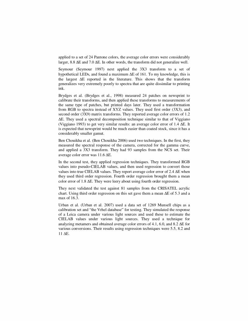
applied to a set of 24 Pantone colors, the average color errors were considerably

larger, 8.8 ∆E and 7.0 ∆E. In other words, the transform did not generalize well.

Seymour (Seymour 1997) next applied the 3X3 transform to a set of

hypothetical LEDs, and found a maximum ∆E of 161. To my knowledge, this is

the largest ∆E reported in the literature. This shows that the transform generalizes very extremely poorly to spectra that are quite dissimilar to printing

ink.

Brydges et al. (Brydges et al., 1998) measured 24 patches on newsprint to

calibrate their transforms, and then applied these transforms to measurements of

the same type of patches, but printed days later. They used a transformation from RGB to spectra instead of XYZ values. They used first order (3X3), and

second order (3X9) matrix transforms. They reported average color errors of 1.2

∆E. They used a spectral decomposition technique similar to that of Viggiano

(Viggiano 1993) to get very similar results: an average color error of 1.4 ∆E. It is expected that newsprint would be much easier than coated stock, since it has a

considerably smaller gamut.

Ben Chouikha et al. (Ben Chouikha 2006) used two techniques. In the first, they

measured the spectral response of the camera, corrected for the gamma curve,

and applied a 3X3 transform. They had 93 samples from the NCS set. Their

average color error was 11.6 ∆E.

In the second test, they applied regression techniques. They transformed RGB

values into pseudo-CIELAB values, and then used regression to convert those

values into true CIELAB values. They report average color error of 2.4 ∆E when they used third order regression. Fourth order regression brought them a mean

color error of 1.8 ∆E. They were leery about using fourth order regression.

They next validated the test against 81 samples from the CRISATEL acrylic

chart. Using third order regression on this set gave them a mean ∆E of 5.3 and a max of 16.3.

Urban et al. (Urban et al. 2007) used a data set of 1269 Munsell chips as a

calibration set and “the Vrhel database” for testing. They simulated the response

of a Leica camera under various light sources and used these to estimate the CIELAB values under various light sources. They used a technique for

analyzing metamers and obtained average color errors of 4.1, 6.0, and 8.2 ∆E for various conversions. Their results using regression techniques were 5.5, 8.2 and

11 ∆E.

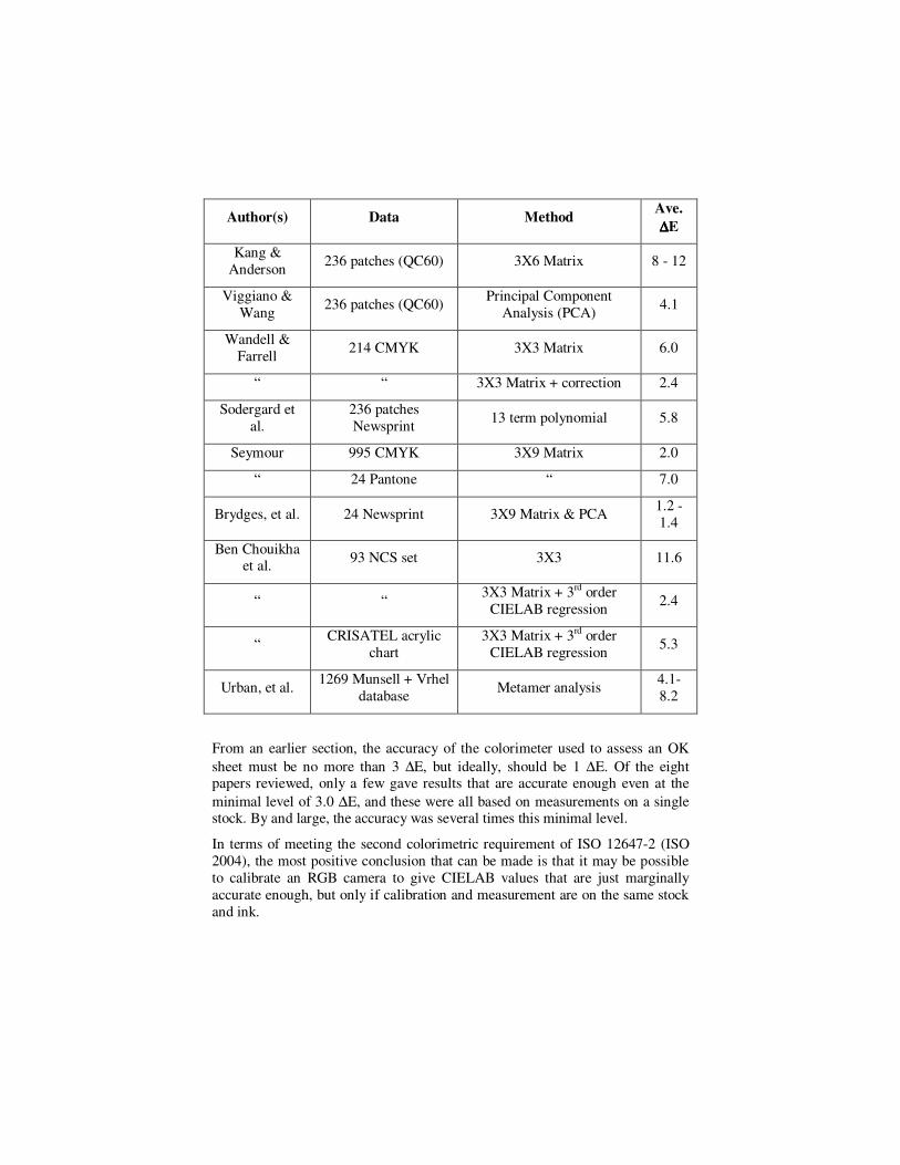
Author(s) Data Method Ave.

∆∆∆∆E

Kang &

Anderson 236 patches (QC60) 3X6 Matrix 8 - 12

Viggiano &

Wang 236 patches (QC60)

Principal Component

Analysis (PCA) 4.1

Wandell &

Farrell 214 CMYK 3X3 Matrix 6.0

“ “ 3X3 Matrix + correction 2.4

Sodergard et

al.

236 patches

Newsprint 13 term polynomial 5.8

Seymour 995 CMYK 3X9 Matrix 2.0

“ 24 Pantone “ 7.0

Brydges, et al. 24 Newsprint 3X9 Matrix & PCA 1.2 -

1.4

Ben Chouikha et al.

93 NCS set 3X3 11.6

“ “ 3X3 Matrix + 3rd order

CIELAB regression 2.4

“ CRISATEL acrylic

chart

3X3 Matrix + 3rd order

CIELAB regression 5.3

Urban, et al. 1269 Munsell + Vrhel

database Metamer analysis

4.1-

8.2

From an earlier section, the accuracy of the colorimeter used to assess an OK

sheet must be no more than 3 ∆E, but ideally, should be 1 ∆E. Of the eight papers reviewed, only a few gave results that are accurate enough even at the

minimal level of 3.0 ∆E, and these were all based on measurements on a single stock. By and large, the accuracy was several times this minimal level.

In terms of meeting the second colorimetric requirement of ISO 12647-2 (ISO

2004), the most positive conclusion that can be made is that it may be possible

to calibrate an RGB camera to give CIELAB values that are just marginally

accurate enough, but only if calibration and measurement are on the same stock

and ink.

Other measures

The previous papers all focused on the accuracy of RGB camera derived

CIELAB measurements. In my review of the literature, I found two papers that

looked at other issues.

Repeatability and reproducibility

An early paper by Simoaa (Simoaa 1987) states that

When compared with discrete photo detectors, the CCD sensors suffer from

rather low signal dynamics, poor noise figures and even low speed due to the serial readout mechanism.

That is to say, the repeatability of CCD devices is inadequate for color

measurement.

Another early paper by Lehtonen (Lehtonen et al, 1991) came to a similar

conclusion:

“These detectors [CCDs] are, however, not efficient enough to meet the

measuring requirements of high-quality prints, in which the black printer may

have a density scale of up to 2.5 D-units.”

A somewhat more recent article in Graphic Arts Monthly (anonymous, 1996)

reiterated these concerns:

“As [Miles Southworth] points out, the thousands of sensors in each camera each has its own gain and color sensitivity. Sometimes each has a signal-to-

noise level that makes it difficult to measure low levels of light accurately.”

None of these papers provided experimental results, so it is hard to determine

how the authors came to their conclusions. The authors evidently did not

consider the benefit of averaging. At any rate, there have been considerable

improvements in the signal quality of CCDs since these papers were published.

Connolly et al. (Connolly 1996) focused on determining the reproducibility of

video cameras. She used a standard 3X3 matrix transform to convert RGB

measurements into XYZ, and took measurements over a period of days. Her

results showed a 0.33 ∆E reproducibility in one test, and 0.19 ∆E in another.

Color difference accuracy

A paper by Tobin et al. (Tobin et al. 2000) looked not at how accurately an RGB

camera can report CIELAB values, but how accurately it can measure ∆E

values.

They used a method called projection onto convex sets to convert RGB values

from a Dalsa camera into CIELAB values. From actual measurements of seven

pairs of similar Pantone patches they computed ∆E values. The errors in

computation of color errors (∆Ecmc) were as large as 2. Their results in measuring spot colors through a textile print run were similar.

A more recent paper by Valencia and Millan (Valencia et al. 2004) investigated

the ability of an RGB camera to reliably distinguish between small color

differences of nearly neutral colors. They measured two sets of Munsell chips:

one set tightly clustered around a pale gray, and the other around a dark grey.

They established that the repeatability of camera measurements for the camera

was quite satisfactory, being less than one tenth of a ∆E. The camera measurements were compared against a spectroradiometer. “The absolute discrepancy between the camera and the reference instrument is less than 0.5

CIELAB units in general”

A related result was reported for the correlation between Status T density

measurements and colorimetric tolerances (Seymour, 2007). The conclusion of

this paper is that changes in Status T density could stand in as a proxy for ∆E during a print run. One would expect that the issues for an arbitrary camera

RGB space would be very similar to those of the Status T color space.

Test of color difference accuracy

From the results of the previous section, it would appear that the accuracy of

RGB camera color difference measurements might be acceptable for verifying

color tolerance within a print run.

Assumptions

The acceptability of an RGB camera depends upon what it is called upon to do.

The assumption is that the camera makes RGB measurements of the printed

work at color ok (that is, when color is deemed acceptable, possibly with a handheld spectrophotometer). Camera CIELAB values are derived from these

RGB measurements and these camera-derived CIELAB values are subsequently

used for comparison against similar measurements taken later in the print run.

The results in this section are not based on direct camera measurements, but

rather on spectral measurements of a large number of samples. I have assumed a

hypothetical spectral response for the camera, and further assumed that all of the

other issues mentioned in section 3 have been properly taking care of.

Data set

A test target of 1,296 patches was printed on a web offset press. The test target

was comprised of all possible combinations of CMYK at 0%, 5%, 25%, 50%,

75%, and solid.

Densities were brought to nominal and a sheet was pulled. The cyan solid ink density was raised by roughly 0.10 D, and another sheet was pulled. The cyan

solid ink density was than lowered to roughly 0.10 D below nominal. In this

way, there were samples of the test target with three different amounts of cyan

ink, much like one might expect through a press run.

Magenta, yellow and black inks were similarly adjusted so that there were nine

sets of targets.

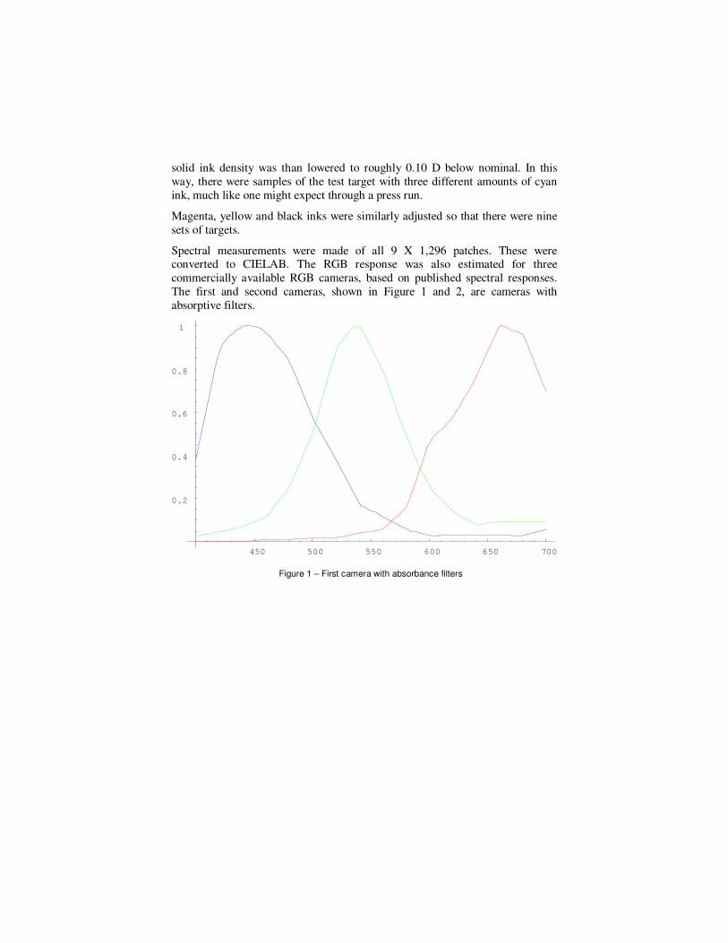
Spectral measurements were made of all 9 X 1,296 patches. These were converted to CIELAB. The RGB response was also estimated for three

commercially available RGB cameras, based on published spectral responses.

The first and second cameras, shown in Figure 1 and 2, are cameras with

absorptive filters.

450 500 550 600 650 700

0.2

0.4

0.6

0.8

1

Figure 1 – First camera with absorbance filters

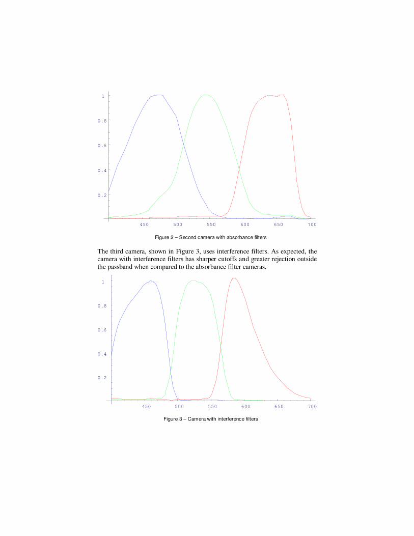
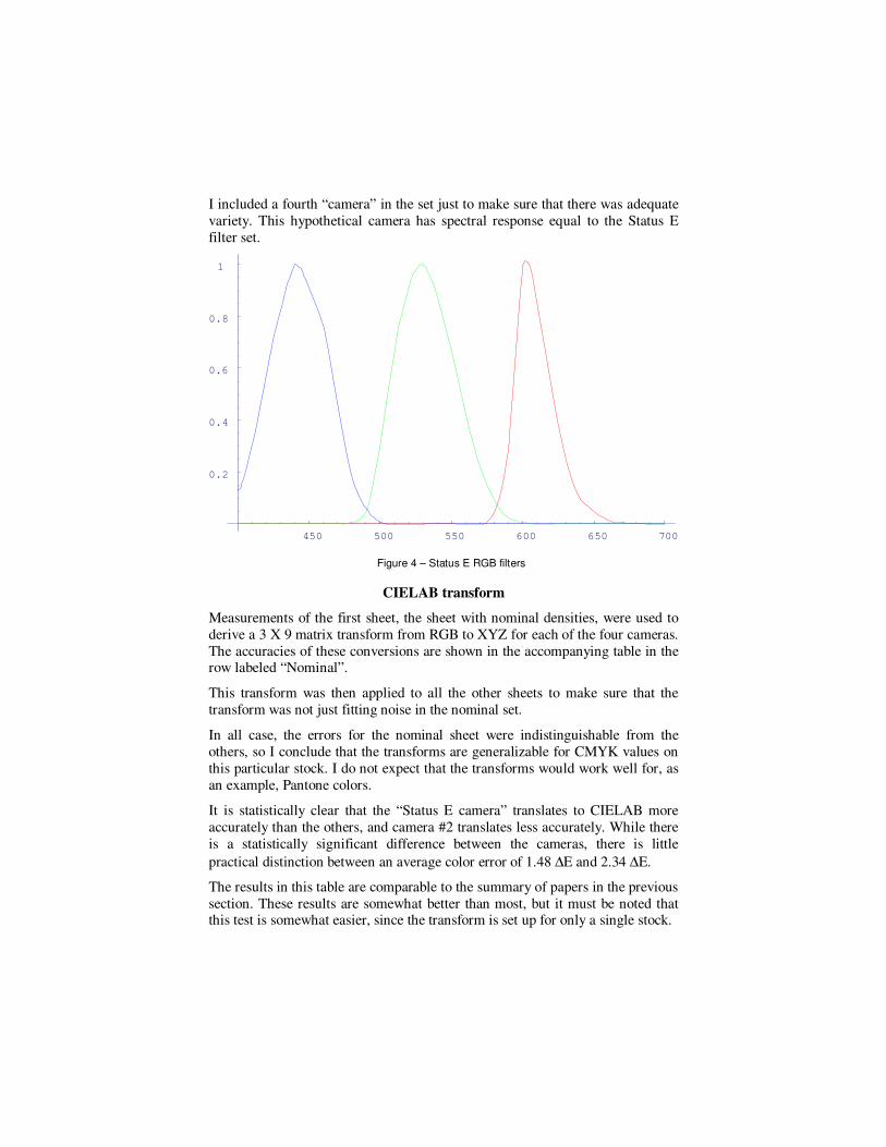
The third camera, shown in Figure 3, uses interference filters. As expected, the camera with interference filters has sharper cutoffs and greater rejection outside

the passband when compared to the absorbance filter cameras.

450 500 550 600 650 700

0.2

0.4

0.6

0.8

1

Figure 3 – Camera with interference filters

Figure 2 – Second camera with absorbance filters

450 500 550 600 650 700

0.2

0.4

0.6

0.8

1

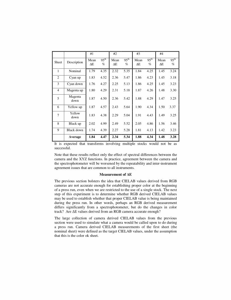
I included a fourth “camera” in the set just to make sure that there was adequate

variety. This hypothetical camera has spectral response equal to the Status E

filter set.

CIELAB transform

Measurements of the first sheet, the sheet with nominal densities, were used to

derive a 3 X 9 matrix transform from RGB to XYZ for each of the four cameras.

The accuracies of these conversions are shown in the accompanying table in the row labeled “Nominal”.

This transform was then applied to all the other sheets to make sure that the

transform was not just fitting noise in the nominal set.

In all case, the errors for the nominal sheet were indistinguishable from the

others, so I conclude that the transforms are generalizable for CMYK values on

this particular stock. I do not expect that the transforms would work well for, as

an example, Pantone colors.

It is statistically clear that the “Status E camera” translates to CIELAB more

accurately than the others, and camera #2 translates less accurately. While there

is a statistically significant difference between the cameras, there is little

practical distinction between an average color error of 1.48 ∆E and 2.34 ∆E.

The results in this table are comparable to the summary of papers in the previous

section. These results are somewhat better than most, but it must be noted that this test is somewhat easier, since the transform is set up for only a single stock.

450 500 550 600 650 700

0.2

0.4

0.6

0.8

1

Figure 4 – Status E RGB filters

#1 #2 #3 #4

Sheet Description Mean

∆E

95th %

Mean

∆E

95th %

Mean

∆E

95th %

Mean

∆E

95th %

1 Nominal 1.79 4.35 2.32 5.35 1.84 4.25 1.45 3.24

2 Cyan up 1.83 4.52 2.36 5.47 1.86 4.23 1.45 3.18

3 Cyan down 1.76 4.27 2.25 5.13 1.86 4.25 1.45 3.23

4 Magenta up 1.80 4.29 2.31 5.18 1.87 4.26 1.48 3.30

5 Magenta

down 1.87 4.50 2.36 5.42 1.88 4.29 1.47 3.25

6 Yellow up 1.87 4.57 2.43 5.64 1.90 4.34 1.50 3.37

7 Yellow down

1.83 4.38 2.29 5.04 1.91 4.43 1.49 3.25

8 Black up 2.02 4.99 2.49 5.52 2.05 4.86 1.56 3.46

9 Black down 1.74 4.39 2.27 5.28 1.81 4.13 1.42 3.23

Average 1.84 4.47 2.34 5.34 1.88 4.34 1.48 3.28

It is expected that transforms involving multiple stocks would not be as

successful.

Note that these results reflect only the effect of spectral differences between the

camera and the XYZ functions. In practice, agreement between the camera and

the spectrophotometer will be worsened by the repeatability and inter-instrument

agreement issues that are common to all instruments.

Measurement of ∆E

The previous section bolsters the idea that CIELAB values derived from RGB

cameras are not accurate enough for establishing proper color at the beginning

of a press run, even when we are restricted to the use of a single stock. The next step of this experiment is to determine whether RGB derived CIELAB values

may be used to establish whether that proper CIELAB value is being maintained

during the press run. In other words, perhaps an RGB derived measurement

differs significantly from a spectrophotometer, but do the changes in color

track? Are ∆E values derived from an RGB camera accurate enough?

The large collection of camera derived CIELAB values from the previous

section were used to simulate what a camera would be called upon to do during

a press run. Camera derived CIELAB measurements of the first sheet (the

nominal sheet) were defined as the target CIELAB values, under the assumption

that this is the color ok sheet.

Color differences were then computed between the nominal set of 1,296 patches

and the 1,296 “cyan +0.1 D” patches, between the nominal and the “cyan -

0.1D”, and so on. This provided eight sets of 1,296 color differences.

There is no particular reason to treat the first sheet as the target. The second

sheet might just as well stand in for the color ok sheet and be compared against

the following seven sheets. With this, we have fifteen (eight plus seven) sets of color differences. In like fashion, the third sheet (“cyan -0.1D”) can be used as

the target, and compared against the remaining six.

All together, it is possible to perform 36 comparisons (8 + 7 + 6 + … + 2 + 1)

between pairs of sheets, simulating a variety of color differences which could

typically occur during a press run. All together, this resulted in 36 X 1,296 =

46,656 color differences.

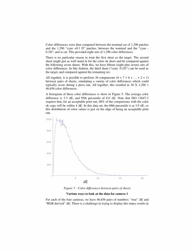
A histogram of these color differences is show in Figure 5. The average color

difference is 3.3 ∆E, and 95th percentile of 8.0 ∆E. Note that ISO 12647-2 requires that, for an acceptable print run, 68% of the comparisons with the color

ok copy will be within 4 ∆E. In this data set, the 68th percentile is at 3.9 ∆E, so this distribution of color values is just on the edge of being an acceptable print

run.

Figure 5 – Color differences between pairs of sheets

Various ways to look at the data for camera 1

For each of the four cameras, we have 46,656 pairs of numbers: “true” ∆E and

“RGB derived” ∆E. There is a challenge in trying to display this many results in

5 10 15 20

200

400

600

800

1000

∆E

a meaningful way, so I will look at the results from one camera, camera 1, in

many different ways.

Note that while the ∆E is never negative, the error can be negative, which is to

say, the RGB derived ∆E would be too large; or the error may be positive, which

is to say the RGB derived ∆E is too small.

The simplest analysis is to use standard statistics. On average, the ∆E values

differ by 0.20 ∆E (the mean of the absolute value of the difference), and 95% of

the errors are less than 0.59 ∆E.

This is acceptable. From section 3.2, we determined that (for ISO 12647-2

compliance) ∆E measurements made by the colorimeter must be accurate to

within 2.4 ∆E and should be accurate to within 0.4 ∆E.

Another way to gauge the agreement between the two measurements of color

difference is to compute the correlation coefficient between them. The

correlation coefficient between the true ∆E values and the RGB derived ∆E values was 0.994, which is an excellent correlation.

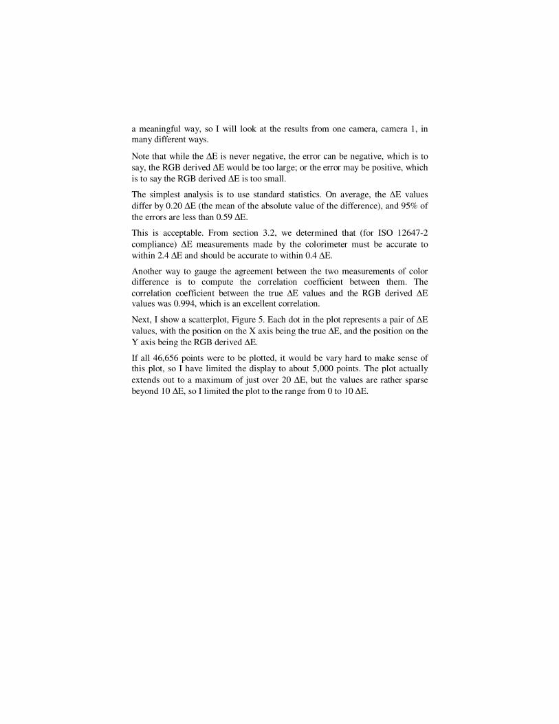
Next, I show a scatterplot, Figure 5. Each dot in the plot represents a pair of ∆E

values, with the position on the X axis being the true ∆E, and the position on the

Y axis being the RGB derived ∆E.

If all 46,656 points were to be plotted, it would be vary hard to make sense of

this plot, so I have limited the display to about 5,000 points. The plot actually

extends out to a maximum of just over 20 ∆E, but the values are rather sparse

beyond 10 ∆E, so I limited the plot to the range from 0 to 10 ∆E.

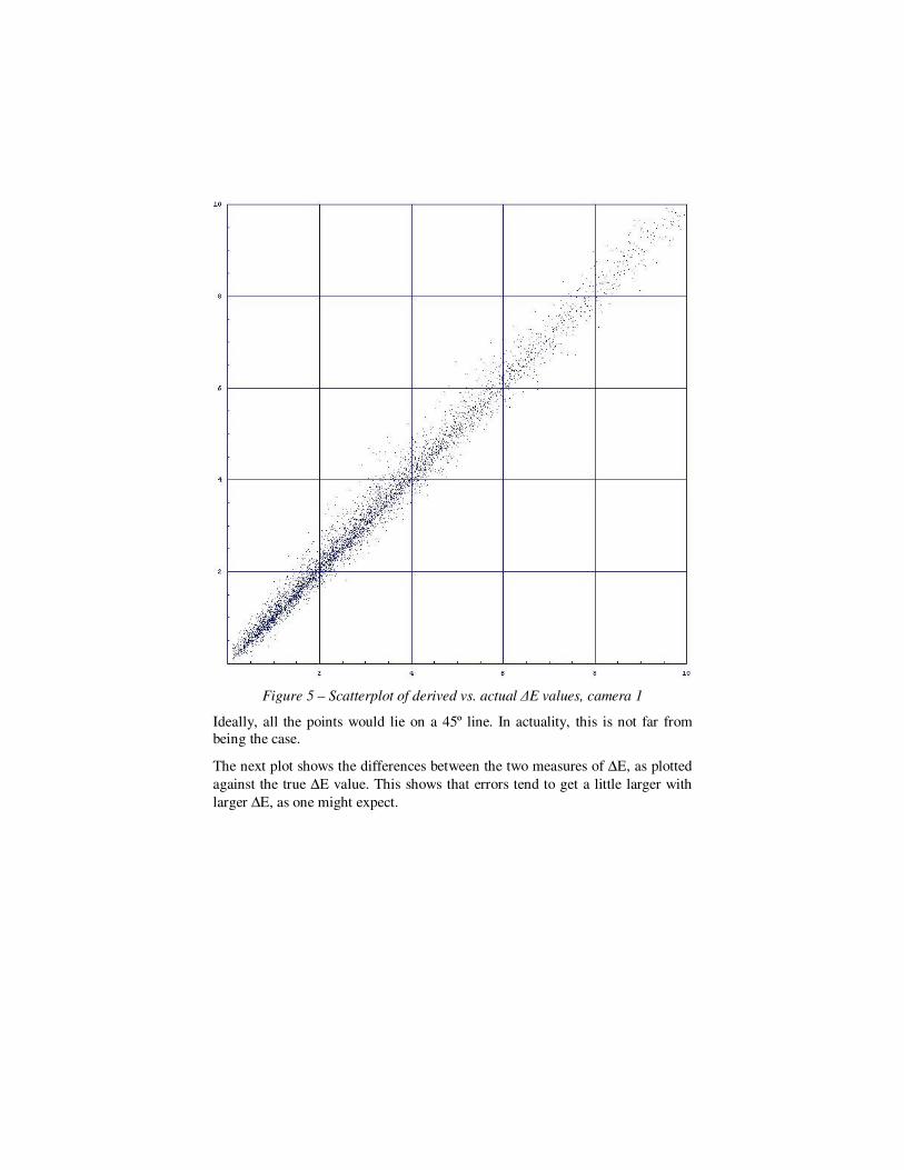
Figure 5 – Scatterplot of derived vs. actual ∆E values, camera 1

Ideally, all the points would lie on a 45º line. In actuality, this is not far from

being the case.

The next plot shows the differences between the two measures of ∆E, as plotted

against the true ∆E value. This shows that errors tend to get a little larger with

larger ∆E, as one might expect.

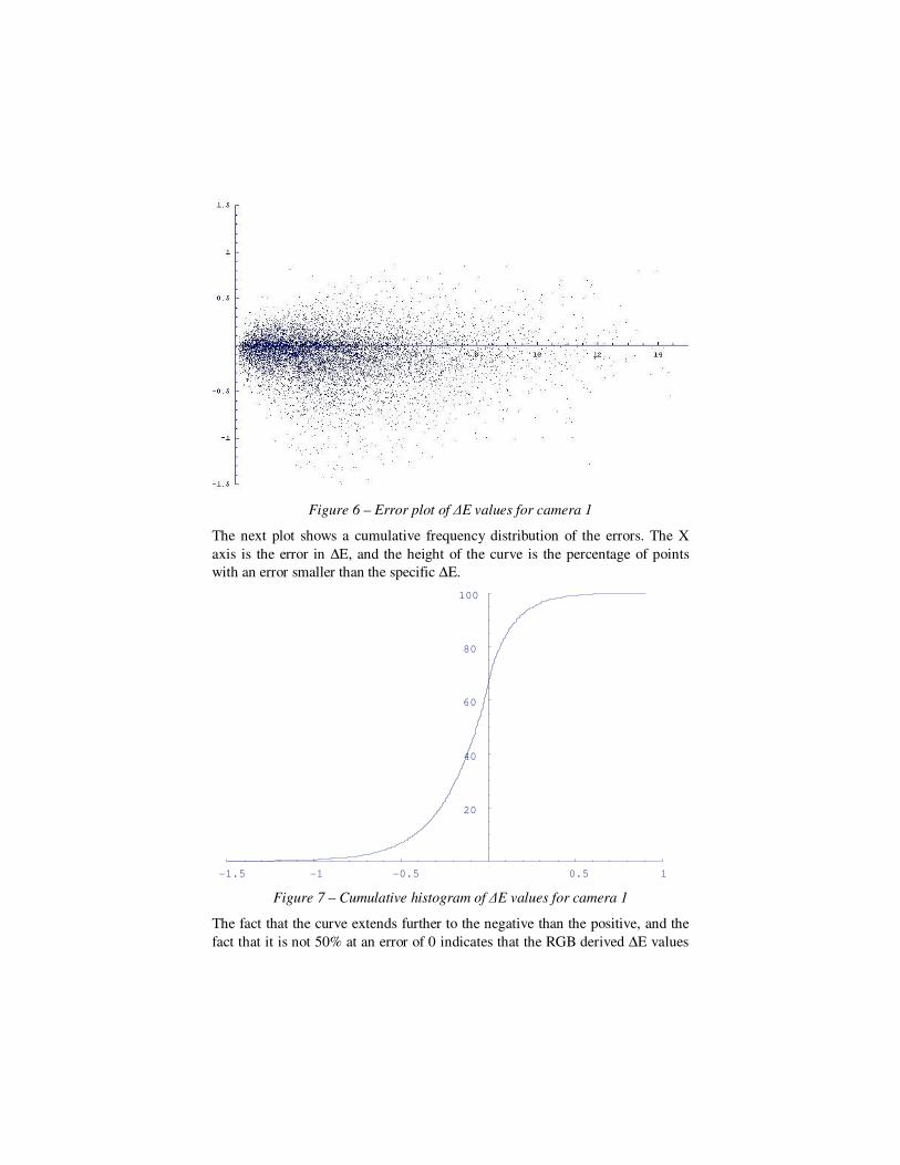
Figure 6 – Error plot of ∆E values for camera 1

The next plot shows a cumulative frequency distribution of the errors. The X

axis is the error in ∆E, and the height of the curve is the percentage of points

with an error smaller than the specific ∆E.

Figure 7 – Cumulative histogram of ∆E values for camera 1

The fact that the curve extends further to the negative than the positive, and the

fact that it is not 50% at an error of 0 indicates that the RGB derived ∆E values

-1.5 -1 -0.5 0.5 1

20

40

60

80

100

tend to run a little larger than the true ∆E values, at least for this particular

camera. (This is not the case for the other cameras.)

False conclusion rate for the four cameras

The previous section helps understand how well the two measurements of ∆E

agree. The real test, though, is how well the RGB derived values work when put

into practice. One important use of these ∆E values during the press run is to determine, on a sheet by sheet basis, which sheets are in compliance, and which

are not. As mentioned before, ISO 12647-2 (ISO 2004) says that 68% of the

sheets must be in compliance. For this purpose, the relevant question is how

often the RGB derived measurements will agree on whether a given

measurement is in tolerance.

For the simulated camera 1 measurements, 66.6% of the time, both the camera

and the spectro agreed that the sample was beyond the 4 ∆E tolerance. The camera and spectro also agreed on classifying 30.2% of the samples as out of

tolerance.

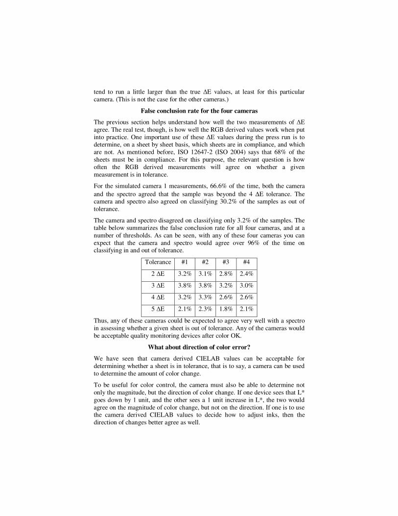
The camera and spectro disagreed on classifying only 3.2% of the samples. The

table below summarizes the false conclusion rate for all four cameras, and at a

number of thresholds. As can be seen, with any of these four cameras you can

expect that the camera and spectro would agree over 96% of the time on classifying in and out of tolerance.

Tolerance #1 #2 #3 #4

2 ∆E 3.2% 3.1% 2.8% 2.4%

3 ∆E 3.8% 3.8% 3.2% 3.0%

4 ∆E 3.2% 3.3% 2.6% 2.6%

5 ∆E 2.1% 2.3% 1.8% 2.1%

Thus, any of these cameras could be expected to agree very well with a spectro

in assessing whether a given sheet is out of tolerance. Any of the cameras would

be acceptable quality monitoring devices after color OK.

What about direction of color error?

We have seen that camera derived CIELAB values can be acceptable for

determining whether a sheet is in tolerance, that is to say, a camera can be used

to determine the amount of color change.

To be useful for color control, the camera must also be able to determine not

only the magnitude, but the direction of color change. If one device sees that L*

goes down by 1 unit, and the other sees a 1 unit increase in L*, the two would

agree on the magnitude of color change, but not on the direction. If one is to use the camera derived CIELAB values to decide how to adjust inks, then the

direction of changes better agree as well.

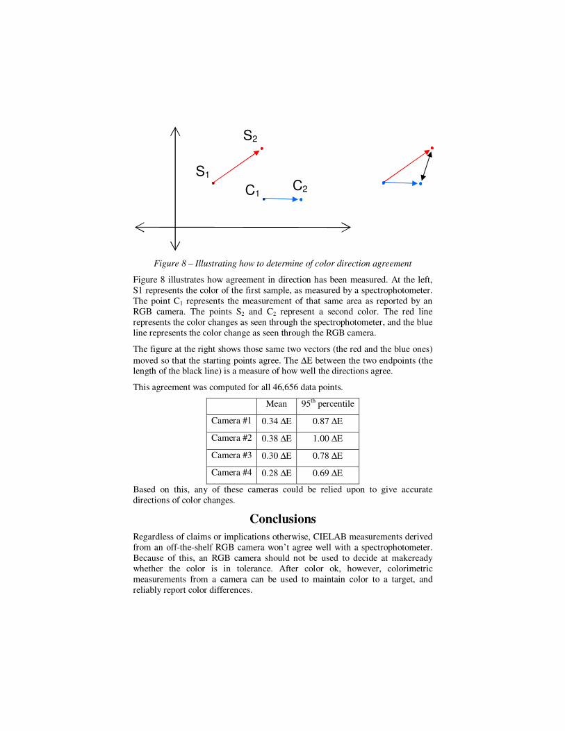
Figure 8 – Illustrating how to determine of color direction agreement

Figure 8 illustrates how agreement in direction has been measured. At the left,

S1 represents the color of the first sample, as measured by a spectrophotometer.

The point C1 represents the measurement of that same area as reported by an

RGB camera. The points S2 and C2 represent a second color. The red line

represents the color changes as seen through the spectrophotometer, and the blue

line represents the color change as seen through the RGB camera.

The figure at the right shows those same two vectors (the red and the blue ones)

moved so that the starting points agree. The ∆E between the two endpoints (the length of the black line) is a measure of how well the directions agree.

This agreement was computed for all 46,656 data points.

Mean 95th percentile

Camera #1 0.34 ∆E 0.87 ∆E

Camera #2 0.38 ∆E 1.00 ∆E

Camera #3 0.30 ∆E 0.78 ∆E

Camera #4 0.28 ∆E 0.69 ∆E

Based on this, any of these cameras could be relied upon to give accurate

directions of color changes.

Conclusions

Regardless of claims or implications otherwise, CIELAB measurements derived

from an off-the-shelf RGB camera won’t agree well with a spectrophotometer.

Because of this, an RGB camera should not be used to decide at makeready

whether the color is in tolerance. After color ok, however, colorimetric

measurements from a camera can be used to maintain color to a target, and

reliably report color differences.

S1

S2

C1 C2

Acknowledgements

I would like to thank my proofreaders: Jeff Bast and Bobbi Olp.

Literature Cited

Anonymous,

1996 “Choosing sensor for press color control”, Graphic Arts Monthly, October, 1996

ASTM

2002 ASTM 2214-02 “Standard Practice for Specifying and Verifying the Performance of Color-Measuring Instruments”

Brydges, D., F. Deppner, H. Kunzli, K. Heuberger, and R.D. Hersch,

1998 “Application of a 3-CCD color camera for colorimetric and densitometric measurements”, SPIE 3300, 1998

Ben Chouikha M. Placais, B., Pouleau, G. Sautot, S., and Vienot, F, Benefits

2006 “Drawbacks of two Methods for Characterizing Digital Cameras”, CGIV 2006 proc. IS&T, p. 185 - 188

Connolly, C., TWW Leung, and JH Nobbs,

1996 “The use of video cameras for remote colour measurement”, JSDC, 112, 1-4, 1996

ISO

1993 ISO VIM, “The International Vocabulary of Basic and General Terms in Metrology”

1983 ISO 5/4:1983, “Photography - Density Measurements - Part 4: Geometric conditions for reflection density”

1996 ISO 12647-1:1996, “Graphic technology - Process control for the manufacture

of half-tone colour separations, proof and production prints - Part 1: Parameters and measurement methods”

1996 ISO 13655:1996, “Graphic technology – Spectral measurement and colorimetric computation for graphic arts images”

2004 ISO 12647-2:2004(E), “Graphic technology – Process control for the production of half-tone colour separations, proof and production prints – Part 2: Offset lithographic processes”

Jansson, Peter and Robert Breault,

1998 “Correcting color-measurement error caused by stray light in image scanners, The Sixth Color Imaging Conference: Color Science, Systems and Applications”, pp. 69-73

Kang, H. R. and P. G. Anderson

1992 “Neural network applications to the color scanner and printer calibrations”, J. Elect. Imaging, vol. 1(2), pp. 125 - 135, April 1992

Lehtonen, T., H. Juhola, R. Launonen, U. Pulkkinen,

1991 “On-press control of the newspaper print quality”, TAGA proceedings 1991

McDowell, David, Robert Chung, and Lingjung Chong,

2005 “Correcting measured colorimetric data for differences in backing materials”, TAGA 2005

Rich, Danny,

2004 “Graphic technology – improving the inter-instrument agreement between spectrocolorimeters”, CGATS white paper

Seymour, Rappette, Vroman, Chu, Moersfelder, Gill and Voss

1995 “System and method of monitoring color in a printing press”, US Patent 5,724,259, filed May 4, 1995

Seymour, John,

1996 “The goniophotometry of printing ink”, TAGA proceedings 1996

1997 “Why Do Color Transforms Work?”, Proc. SPIE Vol. 3018, p. 156-164, 1997

1998 “Standards Considerations for Video Densitometry”, GCA Metrology IV

2007 “How many ∆Es are there in a ∆D?”, TAGA proceedings, 2007

2009 “Color Measurement on a flexo press with an RGB camera”, Flexo Magazine, Feb. 2009

Simomaa, K.,

1987 “Are the CCD sensors good enough for print quality monitoring?”, TAGA proceedings 1987, pps 174-185

Sodergard, Caj, Tapio Lehtonen, Raimo Launonen, and Juuso Aikas,

1995 “A system for inspecting colour printing quality”, TAGA 1995, pps. 620 – 634

Spooner, D.,

1995 “An Anthology of Color Measurement Error Mechanisms”, Society of Plastics Engineers Regional Technical Conference

Tobin, K.W., Jr., M.A. Hunt, J.S. Goddard, Jr., K.W. Hylton, R.K. Richards, M.L. Simpson, D.A. Treece,

2000 “Accommodating multiple illumination sources in an imaging colorimetry environment”, Proceedings of SPIE: Machine Vision Applications in Industrial Inspection VIII, Vol. 3966, January 2000.

Urban, Phillip, Roy S. Berns, Rolf-Rainer Grigat,

2007 “Color Correction by Considering the Distribution of Metamers within the Mismatch Gamut”, Society for Imaging Science and Technology, Fifteenth Color Imaging Conference, 2007

Valencia, Edison, Maria S. Millan Garcia-Verela,

2004 “Measuring small color differences in the nearly neutral region by 3CCD

camera”, SPIE Proceedings volume 5622, 2004

Van Nostrand, D.

1968 Van Nostrand’s Scientific Encyclopedia, D. Van Nostrand Company, Fourth Edition

Viggiano, J. A. Stephen, C. Jeffery Wang

1993 “A Novel Method for colorimetric characterization of scanners”, TAGA 1993

Wandell, Brian A. and J. E. Farrell,

1993 “Water into wine: converting scanner RGB to tristimulus XYZ”, Proc. SPIE

1909, pp. 92 - 101, 1993