Embed Size (px)
Citation preview

I L L I N 0 IUNIVERSITY OF ILLINOIS AT URBANA-CHAMPAIGN
PRODUCTION NOTE
University of Illinois atUrbana-Champaign Library
Large-scale Digitization Project, 2007.
S


ILLINOIS______NIATTURATL HSTORVY
Aquatic Biology Technical Report 87/14
SURVEY
Comparative Analysis of FishPopulations in Illinois Impoundments:
Gear Efficiencies andStandards for Condition Factors
Aquatic Biology SectionTechnical Report
Peter B. Bayley and Douglas J. Austen

Illinois Natural History SurveyAquatic Biology Section Technical Report 87/14
COMPARATIVE ANALYSIS OF FISHPOPULATIONS IN ILLINOIS IMPOUNDMENTS:
Gear Efficiencies and Standards for Condition Factors
Peter B. Bayley and Douglas J. Austen
Robert W. Gorden, HeadAquatic Biology Section
September 1987
Peter B. Bayley, PrincipalnvestigatorAquatic Biology Section
SUMMARY OF PROJECT
The major emphasis of this project was in the design and implementation of afisheries data base, the Fisheries Analysis System (FAS), that would provideinformation for managers and researchers on a long-term basis. The secondary, butno less important, emphasis was to interpret and analyze FAS data at the District andState levels.
An overview of FAS is presented in Aquatic Biology Technical Report 87/10.A description of the fish population survey data processing in the DISTRICT FAS partof the system is described in the form of a manual in Aquatic Biology TechnicalReport 87/11 which results from part of the work required under Jobs 101.1 and101.3. Creel Survey data processing is described in Aquatic Biology TechnicalReport 87/12 and completes the requirements under Jobs 101.1 and 101.3. Thestatewide data base, STATE FAS, is described along with uploading anddownloading procedures in Aquatic Biology Technical Report 87/13 (Jobs 101.4and 101.5). Technical Report 87/14 presents an analysis of efficiencies of gearsused in generating most of the data in FAS and an analysis of standard parametersfor condition factors, resulting from requirements under Jobs 101.2 and 101.6.
This technical report is part of the final report of Project F-46-R, Comparative Analysis ofFish Communities in Impoundments, which was conducted under a memorandum ofunderstanding between the Illinois Department of Conservation and the Board ofTrustees of the University of Illinois. The actual work was performed by the Illinois NaturalHistory Survey, a division of the Department of Energy and Natural Resources. Theproject was supported through Federal Aid in Sport Fish Restoration by the U.S. Fishand Wildlife Service, the Illinois Department of Conservation, and the Illinois NaturalHistory Survey. The form, content, and data interpretation are the responsibility of theUniversity of Illinois and the Illinois Natural History Survey, and not that of the IllinoisDepartment of Conservation.
PREFACE
A large data base describing natural or semi-natural resources is not necessarilyin a form that allows comparative analyses on the raw data. Comparisons among orwithin impoundments often require that the data be standardized. Such data are notachieved by standardizing the sampling procedure alone, when inferences about fishpopulations are required. This report addresses problems that affect thecomparability of fish population abundances and condition factors of fish, issuesthat are important to managers and researchers who use this data base.
Gear efficiency, addressed in the first chapter, is as fundamental to fisheriesmanagement as it is to research in fisheries or fish population dynamics. Comparingpopulations between impoundments or habitats can, without an understanding of theefficiency of the sampling methods, produce conclusions that have nothing to dowith the fish populations, but rather reflect the relative ease of capture by size orspecies of fish in different environments. Environmental factors that are used toexplain a hypothetical biological or fishery effect on a fish population, as measuredby the catch per unit effort, may be the same factors that are causing the effect due toa relationship with the catchability of the fish.
The second chapter contains an analysis of the STATE FAS data base in order todefine standards for parameters used to assess the Le Cren condition factor.Condition factor expresses the average well being of individual fish from apopulation which is independent of the size of the population. Condition factor is acomparative index and therefore requires standard parameters for each species. Webelieve that standards relevant for Illinois waters which express the expectedweight-at-length for each major species is an important tool for impoundmentmanagers.
ACKNOWLEDGMENTS
Valuable field assistance was provided by: Lorrie Crossett, David Dowling,Bob Fields, Mike Hooe, Thomas Kwak, Christine Mayer, Barry Newman, ToddPowless, Gary Senger, and Ted Stork from INHS; and Dale Burkett, Larry Cruse,Gary Lutterbie, Alec Pulley, and Harry Wight from IDOC. Data for condition factoranalyses was provided by IDOC District Managers and Harry Wight. Jana Waitemanaged redactional work on this report.
RECOMMENDATIONS
1. Data from all Illinois impoundments sampled in a standardized manner byIDOC biologists should be contributed to FAS.
2. All ancillary measurements listed in DISTRICT FAS for each sample andimpoundment "station" should be recorded for use in efficiency corrections andhabitat comparisons.
3. All sampling sites are fixed but should be selected without bias towardsparticular habitats associated with large fish concentrations. Sites should berepresentative of the impoundment and should, if possible, be selectedrandomly in the area delimited by each impoundment "station."
4. Electrofishing runs should be made as short as practically possible. Extendedsamples cannot be associated with environmental characteristics needed toreduce bias when correcting for efficiency and to make comparisons amonghabitat classifications. Runs covering 5,100 ft (1,550 m) of shoreline,equivalent to about 30 min. of electrofishing, are recommended. Inferences ofpopulation densities are only possible for a few of the species in inshore areasthat have limited weed cover, moderate depth, are not extremely turbid or clear,have moderate to high conductivities, and are sampled in the fall or spring.Confidence intervals of estimates are strongly affected by the total quantity ofsampling effort and to some extent by the sampling variance due to spatialheterogeneity.
5. The current quantity of sampling effort by gillnet fleets in impoundments isonly appropriate as an indicator of the presence of some fish species that maynot be detected by other methods.
6. The current sampling strategy of minnow seines is barely adequate to assessthe strength of recruitment and inadequate to estimate abundance density.
7. A system of reporting changes to impoundments (including fish stocking andhydrological or thermal alterations) is needed to include these data in STATEFAS.
8. Standards computed for the Le Cren condition factor based on Illinoisimpoundments should be used. Other indices of condition can be computed inDISTRICT FAS for some species for comparison with other published results.
9. Software support for the DISTRICT FAS and STATE FAS components shouldcontinue. Less time-consuming methods of data output should be developedon the downloaded STATE FAS using interface programs on R-BASE SYSTEMV.
Chapter 1
GEAR EFFICIENCIES
INTRODUCTION
A standard fishing gear operated in a consistent manner does not ensure that thecatch per unit effort (CPUE) has a constant relationship with the biomass orabundance of a given fish group. Comparative studies demand that comparablesamples be taken from different impoundments. These water bodies may becomparable in the ecological and fisheries sense, but may have physical differencesthat affect catchability, and hence affect our ability to compare abundance densities.
Many fishery decisions require knowledge of the structure of fish populationsrather than their density. No fishing method provides an unbiased size frequencydistribution because of size selectivity. Consequently, estimates of mortality rates orProportional Stock Density (PSD) are biased by an amount depending on the gear,the species, and the pertinent range of fish lengths.
Most biological surveys in Illinois impoundments depend primarily on theboat-mounted, triple-electrode, 230-V AC electroshocker powered by a 3-phase,3,000-W generator. This unit is supplemented by a variety of other methods,including standard gillnet fleets, minnow seines, passive trap devices (trap, hoop,fyke nets), otter trawl, trammel nets, and rotenone.
Determination of efficiency of a gear type under a given operational moderequires that it be calibrated under field conditions. Normal operation of the gearthat fishes a vulnerable population whose size can be estimated will provideunbiased gear efficiency estimates. The vulnerable population (typically a mixture ofdifferent species) in a pond or a blocked off section of an impoundment can bedetermined by (1) stocking known populations prior to the fishing operation, (2)draining the water body, (3) treatment by rotenone or primacord (explosive) whoseefficiency is also determined, (4) classical mark-recapture methods, or (5) classicalmultiple removal methods.
Method (4) provides very approximate population estimates unless a highproportion of the marked fish can be recaptured. Method (5) requires that all the fishhave an equal probability of capture and that subsequent removals are not affected byeach previous fishing operation, in addition to the high catchability assumption formethod (4) (Bayley 1985). In this study the more convenient methods (1) and (2)were employed where possible, and (3) was employed in numerous coves and someponds in the State, often in conjunction with rotenone treatments for other studies orreclamation projects.
Neither rotenone nor primacord is 100% efficient. The following sectionpresents the results of experiments to determine their efficiencies of these samplingmethods.
1-1
ROTENONE AND PRIMACORD EFFICIENCIES
Methods
The percent recovery of marked fish was used to estimate the efficiencies ofrotenone or primacord for different fish groups and site conditions. Theseefficiencies were then used to estimate the number of fish that were vulnerable tocapture within the enclosure by the principal gear (electroshocker, gillnet fleet, orminnow seine) at the beginning of the experiment. In addition to principal gearcalibration, this study of 31 treated enclosures or ponds (Table 1-1) provides thefirst comprehensive analysis of the effectiveness of rotenone and primacord samplesunder a variety of conditions found in Midwestern impoundments.
The sample from the principal gear supplied the majority of marked fish.Marked fish in good condition were returned to the enclosed water body afteridentification and measurement. If additional fish were needed, supplementaryelectrofishing or seining was carried out in similar habitats adjacent to the calibrationzone. Such additional, marked fish were always a very small proportion of the totalfish within the enclosed area. Marked fish were returned to their respective habitatsin the enclosure.
Coves were isolated using block nets of 0.5-in or 0.75-in. bar mesh. ASCUBA diver inspected the nets to ensure that the lead line was firmly grounded.Often in a cove with two arms, each arm was blocked separately and a thirdenclosure was made at their junction. In these cases, fish were marked differently ineach cove so that escapement could be observed independently of the recapturepercentage in each enclosure. Sometimes enclosures were made withinimpoundments or large coves up to 5.565 ha (15 acres) that were then treated withrotenone or drained. Such enclosures were typically along open shorelines up to adepth of 1-2.5 m. The location and the design of enclosures depended on theprincipal gear being calibrated.
Rotenone was applied as an emulsion mixed with water and spread by apropeller attachment to a concentration of 3 ppm. Some of the rotenone was alsospread by backpack sprayer in shallow areas. Rotenone was detoxified usingpotassium permanganate at 3 ppm after 3-4 h. A curtain of potassium permanganatewas maintained outside the enclosure in case of drifting.
Detonating cord (reinforced primacord, Ensign Bickford Company, 50grains/ft or 10.63 g/m) was negatively buoyant and was suspended in mid-waterusing wooden floats attached at 10-m intervals to the cord. The parallel lines weresecured at the ends to prevent drifting. The layout was very similar to that depictedin Metzger and Shafland (1986) except that we used higher densities of detonatingcord networks. Standard splicing techniques were used to join lines and add branchlines to enter small bays. Detonation was effected by an electric blasting cap andbattery power source.
With one exception, coves or ponds were sampled for at least 3 d including theday of application. Each day's catch was recorded separately. The exception was a2-d, preliminary primacord sample in a cove at Lake Sangchris using a 'low-density'detonating cord arrangement, that assumed a minimum lethal range of 3.5-4 m (i.e.,distance between parallel lines was 7-8 m, distance from shore to line was 3.5-4 m).
1-2
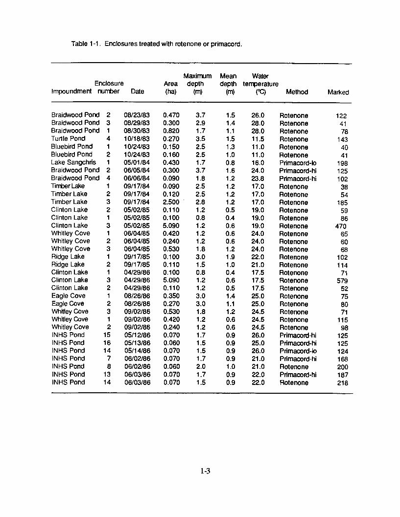
Table 1-1. Enclosures treated with rotenone or primacord.
Maximum Mean WaterEnclosure Area depth depth temperature
Impoundment number Date (ha) (m) (m) (0C) Method Marked
Braidwood Pond 2 08/23/83 0.470Braidwood Pond 3 08/29/83 0.300Braidwood Pond 1 08/30/83 0.820Turtle Pond 4 10/18/83 0.270Bluebird Pond 1 10/24/83 0.150Bluebird Pond 2 10/24/83 0.160Lake Sangchris 1 05/01/84 0.430Braidwood Pond 2 06/05/84 0.300Braidwood Pond 4 06/06/84 0.090Timber LakeTimber LakeTimber LakeClinton LakeClinton LakeClinton LakeWhitley CoveWhitley CoveWhitley CoveRidge LakeRidge LakeClinton LakeClinton LakeClinton LakeEagle CoveEagle CoveWhitley CoveWhitley CoveWhitley CoveINHS PondINHS PondINHS PondINHS PondINHS PondINHS PondINHS Pond
1 09/17/84 0.0902 09/17/84 0.1203 09/17/84 2.5002 05/02/85 0.1101 05/02/85 0.1003 05/02/85 5.0901 06/04/85 0.4202 06/04/85 0.2403 06/04/85 0.5301 09/17/85 0.1002 09/17/85 0.1101 04/29/86 0.1003 04/29/86 5.0902 04/29/86 0.1101 08/26/86 0.3502 08/26/86 0.2703 09/02/86 0.5301 09/02/86 0.4202 09/02/86 0.240
15 05/12/86 0.07016 05/13/86 0.06014 05/14/86 0.070
7 06/02/86 0.0708 06/02/86 0.060
13 06/03/86 0.07014 06/03/86 0.070
3.72.91.73.52.52.51.73.71.82.52.52.81.20.81.21.21.21.83.01.50.81.21.23.03.01.81.21.21.71.51.51.72.01.71.5
1.51.41.11.51.31.00.81.61.21.21.21.20.50.40.60.60.61.21.91.00.40.60.51.41.11.20.60.60.90.90.90.91.00.90.9
26.0 Rotenone28.0 Rotenone28.0 Rotenone11.5 Rotenone11.0 Rotenone11.0 Rotenone16.0 Primacord-lo24.0 Primacord-hi23.8 Primacord-hi17.0 Rotenone17.0 Rotenone17.0 Rotenone19.0 Rotenone19.0 Rotenone19.0 Rotenone24.0 Rotenone24.0 Rotenone24.0 Rotenone22.0 Rotenone21.0 Rotenone17.5 Rotenone17.5 Rotenone17.5 Rotenone25.0 Rotenone25.0 Rotenone24.5 Rotenone24.5 Rotenone24.5 Rotenone26.0 Primacord-hi25.0 Primacord-hi26.0 Primacord-lo21.0 Primacord-hi21.0 Rotenone22.0 Primacord-hi22.0 Rotenone
1-3
1224178
1434041
1981251023854
1855986
470656068
10211471
57952758071
11598
125125124168200187218
Fish retrieval was so poor after 2 d that rotenone was applied. Two more enclosuresat Braidwood Cooling Pond and four INHS ponds were sampled using detonatingcord in a 'high- density' arrangement (effective killing range of 2 m) that was twicethe density used in Lake Sangchris. Fish were retrieved for 3 d. All otherenclosures or impoundments, excluding drainable bodies, were sampled withrotenone because it was cheaper, more convenient, and had higher efficiencies.
Even though the fish were to be subsequently exposed to rotenone orexplosive, considerable care was taken in handling fish for mark and release,because specimens of unnatural buoyancy would likely have different catchabilitiesthan unmarked fish. A galvano-narcotic trough (Blancheteau et al. 1961, Lamarque1963, Hartley 1967) that uses a 48-V DC current to hold fish pointed towards theanode in a state of galvano-narcosis was useful for marking and measuring delicatefish, especially shad, drum, and the young of all species. There is no after-effectand recovery to normal buoyancy and swimming ability is fast.
A recommended chemical dye for fish marking, Bismark Brown Y, wasinvestigated by Bayley (1983), but mortality rates exceeded those of controls whenfish were colored sufficiently to distinguish them. Consequently, we used finclipping as our marking technique. Fish were marked by clipping a third of theupper and/or lower lobe of the caudal fin at an angle of 45°. These clips were mostconvenient to observe recaptured fish, to distinguish them from others with findamage, and to minimize handling during marking. When three contiguousenclosures were used, each was stocked with fish of a different clip combination:upper, lower, or upper and lower. A few species have lobeless caudal fins, such asthe drum. Such individuals >6 cm long could still be clipped in a similar mannerand be subsequently recognized. Fish with forked tailfins >3 cm long were clipped.Fish collected in rotenone or primacord samples were double-checked for marks byexperienced personnel. Many small fish were preserved for later examination toavoid hasty inspection.
We further reduced handling of delicate fish by photographing each batch ofmarked fish in the trough with a centimeter grid on the bottom (Bayley 1983). Thewater level was lowered so that all but very small fish would turn on their sides,permitting species to be identified from the photographs. Numbers and relative sizesof each species within each batch were recorded to check with each photograph.Photographed fish were measured to the extremity of the median rays of the caudalfin. Conversion formulae were used to correct these lengths to compressed totallength for appropriate species, and to correct for a small bias due to the fish beingslightly above the scale. Fish were measured from the photographs using a graphicstablet or electronic calipers that sent the information directly to an Apple //emicrocomputer. These data were converted to unbiased total length estimates byconversion formulae and output for incorporation into the data base. Robust fishwere clipped and measured on a measuring board and recorded manually.
Data Analysis
A total of 4,480 fish were marked or stocked in 36 enclosures (includingponds) (Table 1-1), averaging 124 fish/enclosure. Treating each enclosure as aseparate entity would result in catchability estimates that are too dependent on thevicissitudes of small numbers of fish, particularly when they are broken down into
1-4
length groups and species groups. A more robust efficiency model was sought tocombine data from comparable sets of impoundments and to provide estimates of thevariance of efficiency.
Preliminary data exploration revealed that fish size was an important factordetermining retrieval efficiency (number recaptured x 100/number marked). Clearlyit is not possible to mark constant numbers of fish in given size ranges and species.Retrieval efficiency based on fixed length ranges resulted in highly variable numbersof marked fish per estimate, with estimates for some larger and smaller fish groupsoften based on only a few individuals. Therefore, we grouped fish within lengthranges that were not too wide to mask the effect of length but contained a relativelyconstant number of fish per group.
An algorithm was developed that arranged each marked fish from a sampleaccording to length and split this array into groups of equal numbers of fish. Thiswas done for major species, species groups, and all species combined. Groupnumbers of 10 individuals for species or species groups and 25 individuals for allspecies combined were chosen. A maximum 15-cm length range was permitted fora group. Most groups were much smaller that this limit, but the range of some largerfish attained this limit before the designated group number was reached. In suchcases, a minimum of five individuals per group was used to conserve information onlarger fish. The algorithm progressed from the largest to the smallest marked fish inthe array, assigning recaptured individuals to the appropriate length groups andcalculating efficiencies and mean lengths. If the number of remaining, smallest fishin the array were less than the designated group number, they were added to theprevious group provided that all fish were within the 15-cm range, which wasusually the case. Otherwise, only groups of five individuals or more were used.Mean lengths were calculated for all groups.
This process resulted in a comprehensive data set that permitted the effects offish size, species, and a variety of physical factors on the retrieval efficiency ofrotenone and primacord to be analyzed statistically. The physical factors investigatedincluded those listed in Table 1-1, plus shoreline length, secchi disk readings, a hardcover rating, and a macrophyte cover rating. Analyses of variance (ANOVA) andcovariance (ANCOVA) and multivariate regressions were used to compare retrievalefficiencies of rotenone and primacord with respect to major species or speciesgroups while controlling for the effect of fish size. ANOVA and ANCOVA testswere considered significant at P < 0.05, although most results were significant at P< 0.01. Multiple regression coefficients can be misleading, and a stricter level of P< 0.01 was adopted. Enclosures that had one value with an external studentizedresidual at P < 0.001 were excluded from the model under consideration. Theseenclosures were considered separately. The choice of water bodies and enclosureswas generally dictated by opportunity, available size of block nets, and localphysical conditions, except for the INHS ponds. The ponds are very similar, and arandom allocation of treatments was possible. Therefore, these two sets ofenclosures were analyzed separately.
Results
Preliminary analyses were made with all species combined. Because mostprincipal gear calibrations depended on the non-INHS enclosures that were
1-5
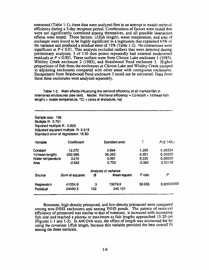
rotenoned (Table 1-1), these data were analyzed first in an attempt to model retrievalefficiency during a 3-day recapture period. Combinations of factors were tested thatwere not significantly correlated among themselves, and all possible interactioneffects were. tested. Three factors: 1/(fish length), water temperature, and area ofenclosure were found to be highly significant in a regression that explained 63% ofthe variance and produced a residual error of 15% (Table 1-2). No interactions weresignificant at P < 0.01. This analysis excluded outliers that were detected duringpreliminary analyses; 3 of 110 data points repeatedly had external studentizedresiduals at P < 0.001. These outliers were from Clinton Lake enclosure 1 (1985),Whitley Creek enclosure 2 (1985), and Braidwood Pond enclosure 3. Higherproportions of fish from the enclosures at Clinton Lake and Whitley Creek escapedto adjoining enclosures compared with other areas with contiguous enclosures.Escapement from Braidwood Pond enclosure 3 could not be estimated. Data fromthese three enclosures were analyzed separately.
Table 1-2. Main effects infuencing the retrieval efficiency of all marked fish inrotenoned enclosures (see text). Model: Retrieval efficiency = Constant + 1/(mean fishlength) + (water temperature, *C) + (area of enclosure, ha)
Sample size: 106Multiple R: 0.791Squared multiple R: 0.626Adjusted squared multiple R: 0.615Standard error of regression: 15.50
Variable Coefficient Standard error T P (2 TAIL)
Constant 12.272 9.564 1.283 0.202341/(mean length) -252.865 36.380 -6.951 0.00000Water temperature 3.219 0.391 8.225 0.00000Area -2.543 0.752 -3.383 0.00102
Analysis of varianceSource Sum-of-squares df Mean-square F-ratio P
Regression 41024.6 3 13674.9 56.955 0.00000000Residual 24490.3 102 240.101
Rotenone, high-density primacord, and low-density primacord were comparedamong non-INHS enclosures and among INHS ponds. The pattern of retrievalefficiency of primacord was similar to that ofrotenone; it increased with increasingfish size and reached a plateau or maximum as fish lengths approached 15-20 cm(Figures 1-1 and 1-2). In ANCOVA tests, the effect of length was accounted for byusing the covariate 1/fish length, because this variable provided the best overall fitamong the three methods.
1-6
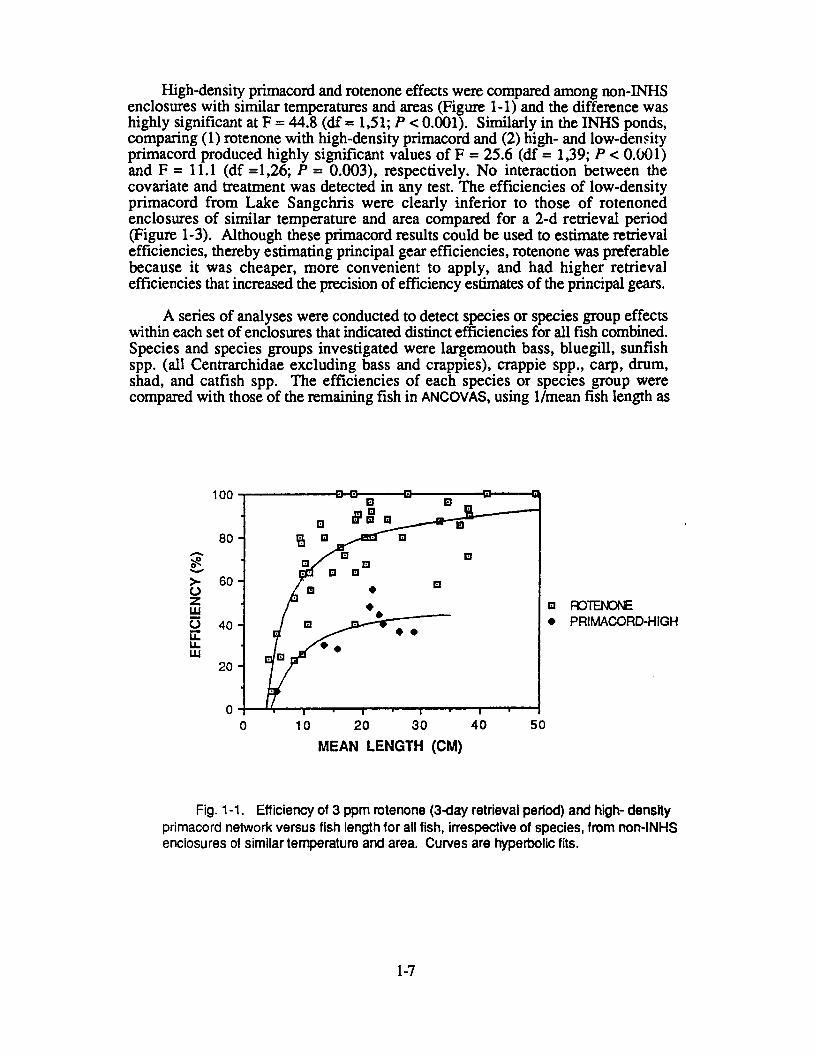
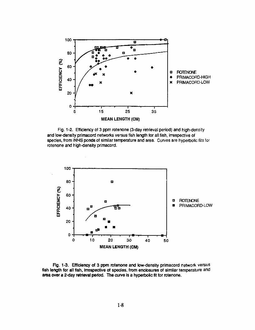
High-density primacord and rotenone effects were compared among non-INHSenclosures with similar temperatures and areas (Figure 1-1) and the difference washighly significant at F = 44.8 (df = 1,51; P < 0.001). Similarly in the INHS ponds,comparing (1) rotenone with high-density primacord and (2) high- and low-densityprimacord produced highly significant values of F = 25.6 (df = 1,39; P < 0.001)and F = 11.1 (df = 1,26; P = 0.003), respectively. No interaction between thecovariate and treatment was detected in any test. The efficiencies of low-densityprimacord from Lake Sangchris were clearly inferior to those of rotenonedenclosures of similar temperature and area compared for a 2-d retrieval period(Figure 1-3). Although these primacord results could be used to estimate retrievalefficiencies, thereby estimating principal gear efficiencies, rotenone was preferablebecause it was cheaper, more convenient to apply, and had higher retrievalefficiencies that increased the precision of efficiency estimates of the principal gears.
A series of analyses were conducted to detect species or species group effectswithin each set of enclosures that indicated distinct efficiencies for all fish combined.Species and species groups investigated were largemouth bass, bluegill, sunfishspp. (all Centrarchidae excluding bass and crappies), crappie spp., carp, drum,shad, and catfish spp. The efficiencies of each species or species group werecompared with those of the remaining fish in ANCOVAS, using 1/mean fish length as
100
80
> 60
LLC.) 4o0U.
20
0
SFOTENONE* PRIMACORD-HIGH
0 10 20 30 40 50
MEAN LENGTH (CM)
Fig. 1-1. Efficiency of 3 ppm rotenone (3-day retrieval period) and high- densityprimacord network versus fish length for all fish, irrespective of species, from non-INHSenclosures of similar temperature and area. Curves are hyperbolic fits.
1-7
SFROTENONE
* PRIMACORD-HIGHx PRIMACORD-LOW
5 15 25 35
MEAN LENGTH (CM)
Fig. 1-2. Efficiency of 3 ppm rotenone (3-day retrieval period) and high-densityand low-density primacord networks versus fish length for all fish, irrespective ofspecies, from INHS ponds of similar temperature and area. Curves are hyperbolic fits forrotenone and high-density primacord.
100-
80-
60-
40-
20 -
0 10 20 30 40
B ROTENONE* PRIMACORD-LOW
50MEAN LENGTH (CM)
Fig. 1-3. Efficiency of 3 ppm rotenone and low-density primacord network versusfish length for all fish, Irrespective of species, from enclosures of similar temperature andarea over a 2-day retrieval period. The curve is a hyperbolic fit for rotenone.
1-8
100
80
600z
40
20
>.
UJE5LLLU
/ Bad
WW
I I I~'0 40 1 I
601101.N
II • I | . I • I I • |
the covariate. Interactions between the treatment (species vs. remainder) and thecovariate were tested; none were significant at P < 0.05. No species or speciesgroup was found to be significantly different (P < 0.05) than the remaining speciesin rotenone or primacord samples in either non-INHS enclosures or INHS ponds,with the single exception of largemouth bass in the low-density primacord sample inLake Sangchris.
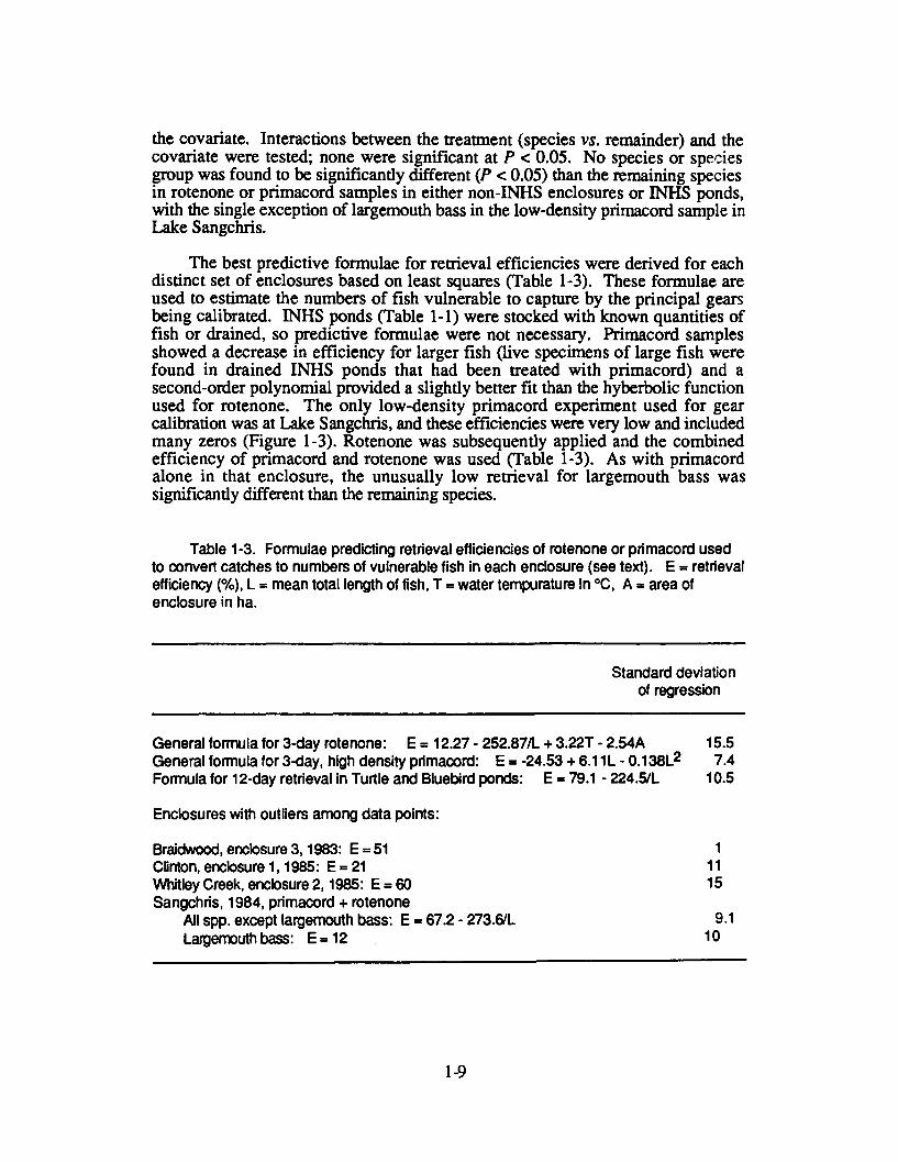
The best predictive formulae for retrieval efficiencies were derived for eachdistinct set of enclosures based on least squares (Table 1-3). These formulae areused to estimate the numbers of fish vulnerable to capture by the principal gearsbeing calibrated. INHS ponds (Table 1-1) were stocked with known quantities offish or drained, so predictive formulae were not necessary. Primacord samplesshowed a decrease in efficiency for larger fish (live specimens of large fish werefound in drained INHS ponds that had been treated with primacord) and asecond-order polynomial provided a slightly better fit than the hyberbolic functionused for rotenone. The only low-density primacord experiment used for gearcalibration was at Lake Sangchris, and these efficiencies were very low and includedmany zeros (Figure 1-3). Rotenone was subsequently applied and the combinedefficiency of primacord and rotenone was used (Table 1-3). As with primacordalone in that enclosure, the unusually low retrieval for largemouth bass wassignificantly different than the remaining species.
Table 1-3. Formulae predicting retrieval efficiencies of rotenone or primacord usedto convert catches to numbers of vulnerable fish in each enclosure (see text). E = retrievalefficiency (%), L = mean total length of fish, T = water tempurature in OC, A = area ofenclosure in ha.
Standard deviationof regression
General formula for 3-day rotenone: E = 12.27 - 252.87/L + 3.22T - 2.54A 15.5General formula for 3-day, high density primacord: E = -24.53 + 6.11L - 0.138L2 7.4Formula for 12-day retrieval in Turtle and Bluebird ponds: E = 79.1 - 224.5/L 10.5
Enclosures with outliers among data points:
Braidwood, enclosure 3,1983: E = 51 1Clinton, enclosure 1, 1985: E = 21 11Whitley Creek, enclosure 2, 1985: E = 60 15Sangchris, 1984, primacord + rotenone
All spp. except largemouth bass: E = 67.2 - 273.6/L 9.1Largemouth bass: E = 12 10
1-9
Constant efficiency and standard deviation estimates were calculated when nofactors were found significant (Table 1-3). The coefficient of variation forlargemouth bass in Lake Sangchris (83%) was considered too high to reliablyestimate the vulnerable population for the electrofishing calibration. Estimates ofvulnerable populations in the enclosures in Turtle and Bluebird ponds were moreprecise when using the higher efficiency data resulting from a 12-d retrieval periodthan those predicted by the general formula, so the appropriate regression in Table1-3 was used in these enclosures.
Discussion
The three, highly significant factors (Table 1-2) have logical explanations.Small fish are generally known to have poor retrieval efficiencies. They undergoerratic, disoriented swimming under the influence of rotenone and tend to get stuckin soft substrates. Such fish are less likely to bloat and rise during the second andthird days than are larger fish. The retrieval procedure was equally thorough for allsizes of fish, and the amount of hard cover or macrophytes were not found to besignificant factors. Smaller fish succumb more quickly and may fall prey to largerfish.
The positive effect of temperature is well known. At higher temperaturesrotenone acts more quickly and fish decompose and bloat rapidly, so that more fishcan be recovered in the first 3 d. The low temperatures at Turtle and Bluebird pondsresulted in only 40% efficiency for large fish after 3 d, but fish rose and could beidentified and measured for another 9 d, resulting in a maximum efficiency of 66%.When the data were reanalyzed excluding these two ponds, the temperature effectwas still significant at P < 0.001.
The negative effect of enclosure area is less easily explained. If area werecorrelated to mean depth, more deep water would result in fewer fish being observedon the bottom that do not subsequently rise. However, area was not correlated withmean depth (P = 0.05) and the latter was not a significant factor in the model (P =0.915). Also, secchi disk reading, affecting visibility of fish on the bottom, was nota significant factor. Less efficient retrieval by a crew covering a larger area mightexplain the effect. However, when persistent winds blew the fish to one bank, suchas in Clinton Lake in 1985, retrieval was easier but retrieval efficiency did notincrease. Other factors that made retrieval tedious, such as macrophyte and hardcover, were not reflected in lower retrieval efficiencies. However, we feel that, ingeneral, manpower limitations in large areas probably contributed to less efficientretrieval. In addition, the highly significant negative effect of area may be due to thedifficulty of attaining an even concentration of rotenone over a large area, resultingin refuges where fish could escape.
The striking differences between primacord and rotenone efficiencies andbetween the two densities of primacord networks was surprising in view of theenthusiasm of Metzger and Shafland (1986) for primacord, even though they used alower density network than the lowest one used in this study. Conditions in Floridawere especially suited for containment of the shock wave: deep channels withvertical limestone walls. Conversely, a windier climate made it more difficult forthem to contain rotenone in an enclosure, although they also found higherefficiencies using rotenone. We found that the lower efficiency of primacord could
1-10
be attributed to an incomplete kill; 20-44% of stocked fish were still alive when theINHS ponds were drained following primacord application, compared with 0% forthose treated with rotenone. Even if primacord had comparable retrieval efficiencies,rotenone is preferable because it is more convenient to set up and is cheaper(including the cost of detoxicant) for the dimensions of enclosures employed heie.
EFFICIENCIES OF THE BOAT ELECTROSHOCKER
Introduction
The boat-mounted, triple-electrode, 230-V AC electroshocker powered by a3-phase, 3,000-W generator is consistently used for sampling impoundments byIDOC and INHS. Each phase is connected to an electrode; the boat itself is notconnected. One dipper and a boatman controlling the outboard motor comprise thecrew; the boatman also dips fish. Flexible copper-based conduit electrodes wereused in these experiments, which are used by INHS and a majority of IDOCpersonnel. The electrodes are cleaned with abrasive paper regularly to maintaingood conductance in water. Although some IDOC personnel use stiff, copper rods,we believe that the flexible, unweighted electrodes, which drop more easily intowoody habitats, should be the standard.
Differences between personnel and type of generator may affect catchability.We tested the two common generators used that conform to the abovespecifications--Homelite and Kohler. Also, many samples were taken by IDOCpersonnel. However, comparable equipment does not ensure comparableefficiencies. These experiments conformed to IDOC recommendations on samplingmethods that, in fact, represent the existing practice of most personnel. The majorissues are distance versus time as a measure of effort, the average speed of approachto new habitat, and distance offshore. A standardized sample should cover a givendistance, including habitats representative of the impoundment. Because the normalpractice is to "circle back" to pick up stunned fish that, due to local concentrations,could not be picked up on the first pass, using time as a unit of effort results in a
1600
1200
I-z-_ 800
0 400
0
0 BLOCKED AREAS* PONDS* LARGE LAKES
0 10 20 30 40 50 60 70 80
DURATION (MIN)
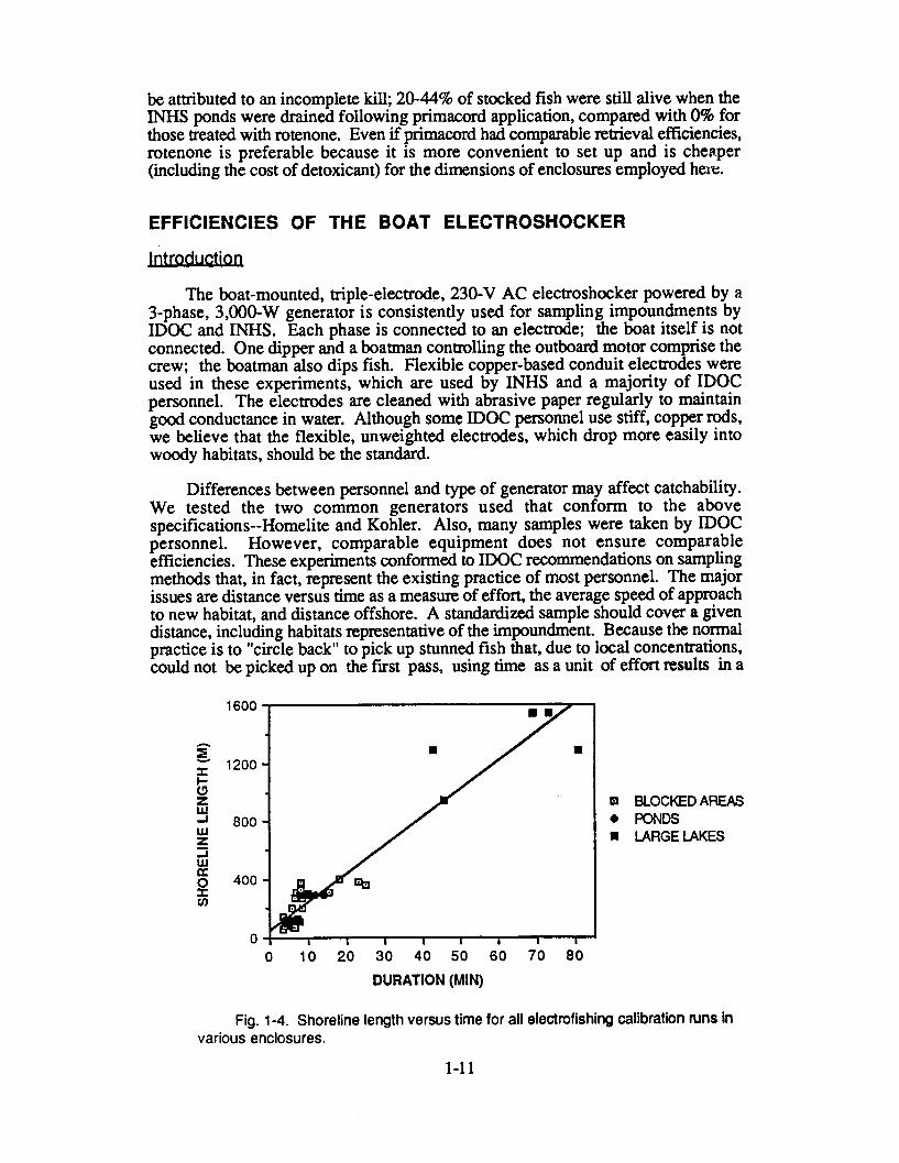
Fig. 1-4. Shoreline length versus time for all electrofishing calibration runs invarious enclosures.
1-11

CPUE index that underestimates fish density when large quantities are encountered.Time is important, however, with respect to the speed of covering new water. Afaster speed generally produces more large fish, except where such good habitats asbrush piles occur, which are fished at a slower speed. The plot of distance versustime for 59 electrofishing calibrations (Figure 1-4) is remarkably consistentconsidering the potential for variation; no differences were detected between INHSand IDOC boatmen. The average speed for all runs was 0.43 m/sec (±0.15 SD).Distance of the boat from the shoreline depends on sufficient water depth. Exceptfor shallow areas that do not permit the outboard motor to clear the bottom, thedistance is close enough so that the dipper can just reach the water's edge unlessexcessive weeds are present.
Our calibrations simulated this process during fall and spring when regularelectrofishing surveys occur. They cannot be applied to other times of the year,when the inshore/offshore distribution of many fish species differs and otherphysical conditions outside the ranges tested may occur.
Efficiency and Design
The efficiency of the standard gear is the proportion of a given species and sizegroup of fish that is removed from a given area by a standard fishing operation asdescribed above. In the experiments, the given area is the one within which thevulnerable population is estimated. This area may be a whole water body that hasbeen drained or rotenoned, or an area blocked off from a larger impoundment thathas been subsequently treated with rotenone or primacord.
The ratio of the area to the shoreline length, which is equivalent to the meanwidth of the sample run, is important. The boat electrofisher fishes a relativelynarrow band along the shoreline. Therefore, the efficiency relative to an area withina defined distance from shore, called the inshore zone, may be different than thatrelative to the whole impoundment. The difference will depend on the proportion offish outside the inshore zone. Comparing a series of large water bodies of varyingarea to shoreline ratios may be feasible when the fish concerned are known tooccupy only the inshore area, such as the young walleye in Sern's (1978)calibrations. Otherwise, inshore factors that affect catchability may be confusedwith the inshore/offshore distribution, which affects vulnerability to the gear.Moreover, a larger set of factors may be responsible for overall lake catchabilitywhich would be difficult to unravel in a multivariate analysis from a limited numberof samples. Conversely, a larger number of inshore zone calibrations are possibleunder a given budget and a smaller number of factors affecting catchability need tobe assessed. This advantage must be compared to the desirability of predictingabundance in large water bodies. The inshore zone calibrations cannot do thisexcept for very small or narrow water bodies of similar area to shoreline ratios, butthey can provide a basis for comparing abundances among inshore habitats in thesame or different lakes.
This study, having no precedents, concentrated on inshore zone calibrations(54) but also included five 'large water-body' calibrations in impoundments (Tables1-4 and 1-5). This analysis concentrates on the inshore calibrations. A preliminaryanalysis of the large water-body calibrations is presented; a more detailed analysisawaits sampling variance data from similar waters across Illinois.
1-12
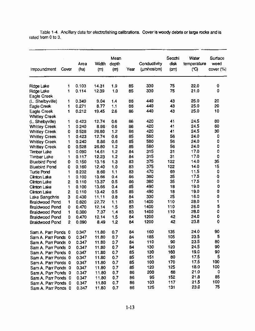
Table 1-4. Ancillary data for electrofishing calibrations. Cover is woody debris or large rocks and israted from 0 to 3.
Impoundment Cover
MeanArea Width depth(ha) (m) (m)
ConductivityYear (gmhos/cm)
Secchidisk(cm)
Watertemperature
(CC)
Ridge LakeRidge LakeEagle Creek(L. Shelbyville)Eagle CreekEagle CreekWhitley Creek(L. Shelbyville)Whitley CreekWhitley CreekWhitley CreekWhitley CreekWhitley CreekTimber LakeTimber LakeBluebird PondBluebird PondTurtle PondClinton LakeClinton LakeClinton LakeClinton LakeLake SangchrisBraidwood PondBraidwood PondBraidwood PondBraidwood PondBraidwood Pond
Sam A. Parr PondsSam A. Parr PondsSam A. Parr PondsSam A. Parr PondsSam A. Parr PondsSam A. Parr PondsSam A. Parr PondsSam A. Parr PondsSam A. Parr PondsSam A. Parr PondsSam A. Parr PondsSam A. Parr Ponds
I1
11I
1101I01100I1212310I02
000000000000
0.103 14.31 1.90.114 12.39 1.0
0.3490.2710.212
0.4230.2400.5280.4230.2400.5280.0900.1170.1500.1600.2020.1000.1100.1000.1100.4300.8200.4700.3000.4700.090
0.3470.3470.3470.3470.3470.3470.3470.3470.3470.3470.3470.347
9.048.77
19.45
12.748.86-
26.8012.748.86
26.8014.6112.2313.1612.408.60
13.6613.3713.6613.4211.1122.7212.14
7.3712.14
8.49
11.8011.8011.8011.8011.8011.8011.8011.8011.8011.8011.8011.80
1.41.12.6
0.60.61.20.60.61.21.21.21.31.01.10.40.50.40.50.81.11.51.41.51.2
0.70.70.70.70.70.70.70.70.70.70.70.7
Surfaceweed
cover (%)
8585
868686
868686858585848483838386868585848383838484
848484848585858586868686
330330
440440440
420420420580580580315315375375470380380490490330
14001400140012001200
16018511013013015110012020095
103125
7575
434343
4141415656563131
122122693535181825
1101101104242
13510590
12016080
17012568
152117131
22.021.0
25.025.025.0
24.524.524.524.024.024.017.017.014.014.011.517.517.519.019.016.028.026.028.024.023.8
24.023.523.524.519.017.517.518.021.021.821.523.0
00
202010
806030
000003515
00000015000
905
809090
5100100
085
10075
1-13
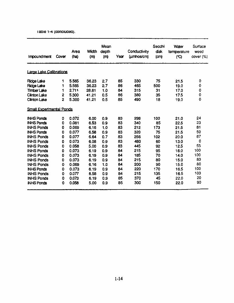
Saoie 1-4 (concluoeo).
Mean Secchi Water SurfaceArea Width depth Conductivity disk temperature weed
Impoundment Cover (ha) (m) (m) Year (pmhos/cm) (cm) (OC) cover (%)
Large Lake Calibrations
Ridge Lake 1 5.565 36.23 2.7 85 330 75 21.5 0Ridge Lake 1 5.565 36.23 2.7 86 465 500 19.0 0Timber Lake 1 2.711 28.81 1.0 84 315 31 17.0 0Clinton Lake 2 5.300 41.21 0.5 86 380 35 17.5 0Clinton Lake 2 5.300 41.21 0.5 85 490 18 19.0 0
Small Experimental Ponds
INHS Ponds 0 0.072 6.00 0.9 83 298 100 21.0 24INHS Ponds 0 0.081 6.53 0.9 83 340 85 22.5 23INHS Ponds 0 0.069 6.16 1.0 83 212 173 21.5 81INHS Ponds 0 0.077 6.58 0.9 83 320 75 21.5 50INHS Ponds 0 0.077 6.64 0.7 83 256 102 20.0 87INHS Ponds 0 0.073 6.08 0.9 83 480 60 13.0 0INHS Ponds 0 0.058 5.00 0.9 83 445 92 12.5 55INHS Ponds 0 0.073 6.19 0.9 84 215 95 16.0 100INHS Ponds 0 0.073 6.19 0.9 84 185 70 14.0 100INHS Ponds 0 0.073 6.19 0.9 84 215 80 15.0 80INHS Ponds 0 0.069 6.16 1.0 84 200 90 15.0 80INHS Ponds 0 0.073 6.19 0.9 84 220 170 16.5 100INHS Ponds 0 0.077 6.58 0.9 84 215 135 16.5 100INHS Ponds 0 0.073 6.19 0.9 85 370 45 22.0 20INHS Ponds 0 0.058 5.00 0.9 85 300 150 22.0 90
1-14
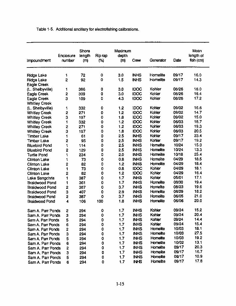
Table 1-5. Additional ancillary for electrofishing calibrations.
Shore Maximum MeanEnclosure length Rip rap depth length of
Impoundment number (m) (%) (m) Crew Generator Date fish (cm)
Ridge LakeRidge LakeEagle Creek(L. Shelbyville)Eagle CreekEagle CreekWhitley Creek(L. Shelbyville)Whitley CreekWhitley CreekWhitley CreekWhitley CreekWhitley CreekTimber LakeTimber LakeBluebird PondBluebird PondTurtle PondClinton LakeClinton LakeClinton LakeClinton LakeLake SangchrisBraidwood PondBraidwood PondBraidwood PondBraidwood PondBraidwood Pond
Sam A. Parr PondsSam A. Parr PondsSam A. Parr PondsSam A. Parr PondsSam A. Parr PondsSam A. Parr PondsSam A. Parr PondsSam A. Parr PondsSam A. Parr PondsSam A. Parr PondsSam A. Parr PondsSam A. Parr Ponds
12
123
I23I23I212112I21I2324
235623562356
7292
386309109
3322711973322711976195
11412923473827382
387361387407387106
294294294294294294294294294294294294
00
000
000-00000000000000000
100
000000000000
3.0 INHS Homelite1.5 INHS Homelite
3.0 IDOC Kohler3.0 IDOC Kohler4.3 IDOC Kohler
1.2 IDOC Kohler1.2 IDOC Kohler1.8 IDOC Kohler1.2 IDOC Kohler1.2 IDOC Kohler1.8 IDOC Kohler2.5 INHS Kohler2.5 INHS Kohler2.5 INHS Homelite2.5 INHS Homelte2.0 INHS Homelite0.8 INHS Homelite1.2 INHS Homelite0.8 IDOC Kohler1.2 IDOC Kohler1.7 INHS Kohler1.7 INHS Homelite3.7 INHS Homelte2.9 INHS Homelite3.7 INHS Homelite1.8 INHS Homelite
1.7 INHS Kohler1.7 INHS Kohler1.7 INHS Kohler1.7 INHS Kohler1.7 INHS Homelte1.7 INHS Homelite1.7 INHS Homelite1.7 INHS Homelite1.7 INHS Homelite1.7 INHS Homelite1.7 INHS Homehte1.7 INHS Homelite
1-15
09/1709/17
08/2608/2608/26
09/0209/0209/0206/0306/0306/0309/1709/1710/2410/2410/1804/2904/2904/2904/2905/0108/3008/2308/2906/0506/06
09/2409/2409/2409/2410/0310/0310/0310/0209/1709/1709/1709/17
16.014.3
16.016.417.2
16.614.715.018.719.320.523.419.215.013.325.418.518.418.116.417.119.419.618.221.020.0
15.220.414.415.418.127.519.213.120.316.710.917.8
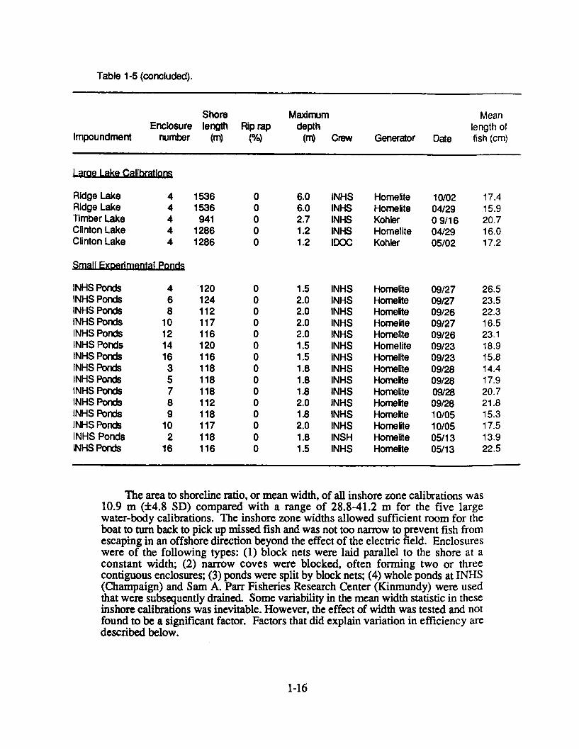
Table 1-5 (concluded).
Shore Maximum MeanEnclosure length Rip rap depth length of
Impoundment number (m) (%) (m) Crew Generator Date fish (cm)
Large Lake Calibrations
Ridge Lake 4 1536 0 6.0 INHS Homelite 10/02 17.4Ridge Lake 4 1536 0 6.0 INHS Homelite 04/29 15.9Timber Lake 4 941 0 2.7 INHS Kohler 09/16 20.7Clinton Lake 4 1286 0 1.2 INHS Homelite 04/29 16.0Clinton Lake 4 1286 0 1.2 IDOC Kohler 05/02 17.2
Small Experimental Ponds
INHS Ponds 4 120 0 1.5 INHS Homelite 09/27 26.5INHS Ponds 6 124 0 2.0 INHS Homelite 09/27 23.5INHS Ponds 8 112 0 2.0 INHS Homelite 09/26 22.3INHS Ponds 10 117 0 2.0 INHS Homelite 09/27 16.5INHS Ponds 12 116 0 2.0 INHS Homelite 09/26 23.1INHS Ponds 14 120 0 1.5 INHS Homelite 09/23 18.9INHS Ponds 16 116 0 1.5 INHS Homerite 09/23 15.8INHS Ponds 3 118 0 1.8 INHS Homelte 09/28 14.4INHS Ponds 5 118 0 1.8 INHS Homelite 09/28 17.9INHS Ponds 7 118 0 1.8 INHS Homelite 09/28 20.7INHS Ponds 8 112 0 2.0 INHS Homelite 09/28 21.8INHS Ponds 9 118 0 1.8 INHS Homelite 10/05 15.3INHS Ponds 10 117 0 2.0 INHS Homelite 10/05 17.5INHS Ponds 2 118 0 1.8 INSH Homelite 05/13 13.9INHS Ponds 16 116 0 1.5 INHS Homelite 05/13 22.5
The area to shoreline ratio, or mean width, of all inshore zone calibrations was10.9 m (±4.8 SD) compared with a range of 28.8-41.2 m for the five largewater-body calibrations. The inshore zone widths allowed sufficient room for theboat to turn back to pick up missed fish and was not too narrow to prevent fish fromescaping in an offshore direction beyond the effect of the electric field. Enclosureswere of the following types: (1) block nets were laid parallel to the shore at aconstant width; (2) narrow coves were blocked, often forming two or threecontiguous enclosures; (3) ponds were split by block nets; (4) whole ponds at INHS(Champaign) and Sam A. Parr Fisheries Research Center (Kinmundy) were usedthat were subsequently drained. Some variability in the mean width statistic in theseinshore calibrations was inevitable. However, the effect of width was tested and notfound to be a significant factor. Factors that did explain variation in efficiency aredescribed below.
1-16
Analysis and Results
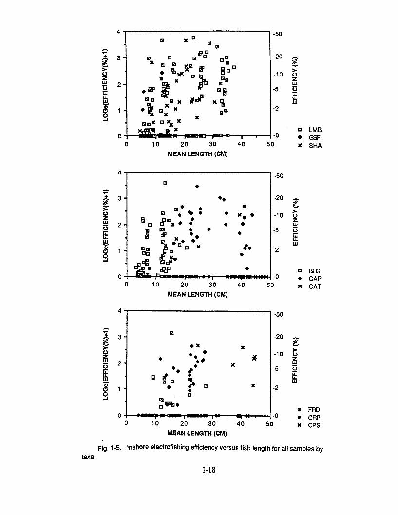
The number of possible approaches to the analysis of this large, complex dataset is almost infinite. Attempts to stabilize the variability, such as combining speciesof similar catchability or combining fish within large length groups, had to bebalanced by the need to find differences due to taxa, fish size, and ancillary factors.The large numbers of vulnerable fish precluded the necessity of dealing with variablelength groups, as was the case with the limited quantities of marked fish used in therotenone/primacord estimates. Four length groups (0-9.99, 10-19.9, 20-29.99, and30+ cm) were used in inshore calibrations; the mean length was calculated from thelength frequency of vulnerable fish within each group. Whole water-bodycalibrations produced sufficiently large quantities of fish to use 7 length groups:0-9.99, 10-14.99, 15-19.99, 20-24.99, 25-29.99, 30-39.99, 40+ cm. As with themarked fish analysis, efficiency estimates based on fewer than five recovered fishwere not included in the analysis. In addition to all species combined, nine taxawere analyzed: largemouth bass (LMB), bluegill (BLG), green sunfish (GSF),freshwater drum (FRD), shad spp. (SHA), carp (CAP), crappie spp. (CRP), catfishspp. (CAT: channel catfish and yellow and black bullheads), and carpsucker spp.(CPS: mostly quillback, river carpsucker, some redhorse and buffalo spp.).
Preliminary analyses revealed that the distributions of efficiencies werestrongly positively skewed. These were normalized by a log transformation ofefficiency as a percentage after adding 1 to allow transformation of zero efficiencies.Figures show the transformed data as the ordinate, and untransformed efficienciesare shown on the right of each graph. All data plotted by length and taxa werehighly variable (Figure 1-5) but various independent factors could explain asignificant part of the variance in log(efficiency + 1).
Because of the inevitable interaction between taxa and mean length, groups ofuncorrelated ancillary factors (Tables 1-4 and 1-5) were initially tested in multiplecorrelations with efficiencies of all fish, regardless of species, pooled in respectivelength groups. All regressions were checked for first-order interactions and those atP < 0.05 are indicated. Efficiency was not influenced by temperatures, secchi diskvalues, conductivities, hard cover ratings, enclosed areas, or area to shoreline lengthratios (mean width) encountered in these experiments. Anomolously low efficiencieswere obtained from the 0.09-ha enclosure in Timber Lake, which was the smallestblocked area with a very short shoreline. Data from this enclosure were excludedfrom the analysis. Results were highly variable for the INHS ponds but thisvariability could not be explained by any factor. This could be attributed to theirsmall area and the limited numbers of fish of restricted length ranges; therefore,INHS pond data were excluded from this series of analyses.
Conversely, the larger ponds at the Sam A. Parr Fisheries Research Center andthe blocked enclosures showed highly significant effects of mean fish length, meanfish length squared, and percentage surface weed cover (Table 1-6). Thecoefficients of these predictors and the residual error were very similar. In addition,mean depth was highly significant in blocked enclosures (it was constant in theponds). Analyses of other, uncorrelated ancillary factors revealed no significanteffects as was the case with the entire data set including INHS ponds. There was nodifference (P = 0.295) between the efficiencies of the Sam A. Parr ponds andblocked enclosures in an analysis of covariance, using the four factors as covariates.
1-17
÷ 3
z5 2
-Imi
3
00 o
zuJ
ELU
0 LMB* GSF
0 10 20 30 40 50 x SHAMEAN LENGTH (CM)
4
3
zoLU
LU
0 10 20 30
MEAN LENGTH (CM)
+
*
E5Vz3L
00I0-J
3-
2-
1-
00 10 20 30 40
40 5
5
-50
-20 o
-10z
-5 5U-UJ
* BLG* CAPx CAT
-2
-0
-50
-20
-10 0LU
-5 5I-mU.LU
-2
0 FRD* CRPx CPS
-00o
MEAN LENGTH (CM)
Fig. 1-5. Inshore electrofishing efficiency versus fish length for all samples bytaxa.
1-18
0 *
R*im0 * % * * x *
0a I? * ? * *0 a- * *M }°'" x *-
OpMs^[CalB___»«
*x x
m~b,
6domols" SIAMAL AM x.
m
----
*
*50
4
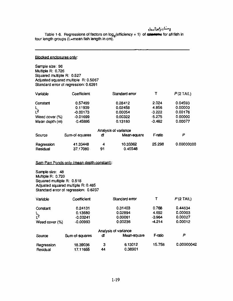
Table 1-6. Regressions of factors on loge(efficiency + 1) of e -tnee for all fish infour length groups (L=mean fish length in cm).
Blocked enclosures only:
Sample size: 96Multiple R: 0.726Squared multiple R: 0.527Adjusted squared multiple R: 0.5067Standard error of regression: 0.6391
Variable
ConstantLL2
Weed cover (%)Mean depth (m)
Source
RegressionResidual
Coefficient
0.574990.11939
-0.00173-0.01699-0.45895
Sum-of-squares
41.3344837.17080
Standard error
0.284120.024580.000540.003220.13180
Analysis of variancedf Mean-square
491
10.333620.45548
T
2.0244.856
-3.222-5.275-3.482
F-ratb
25.298
P (2 TAIL)
0.045930.000000.001760.000000.00077
P
0.00000000
Sam Parr Ponds only (mean depth constant:
Sample size: 48Multiple R: 0.720Squared multiple R: 0.518Adjusted squared multiple R: 0.485Standard error of regression: 0.6237
Variable
ConstantLL2Weed cover (%)
Source
RegressionResidual
Coefficient
0.241310.13580-0.00241-0.00993
Sum-of-squares
18.3903617.11655
Standard error
0.314030.028940.000610.00236
Analysis of variancedf Mean-square
344
6.130120.38901
T
0.7684.692-3.964-4.214
F-ratio
15.758
P (2 TAIL)
0.446340.000030.000270.00012
P
0.00000042
1-19
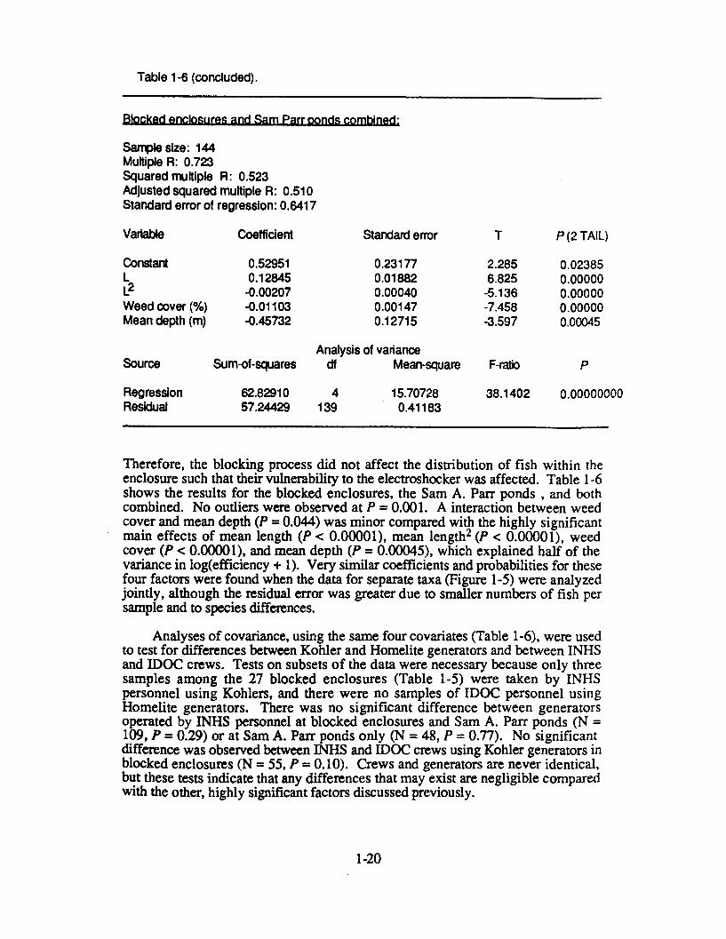
Table 1-6 (concluded).
Blocked enclosures and Sam Parr ponds combined:
Sample size: 144Multiple R: 0.723Squared multiple R: 0.523Adjusted squared multiple R: 0.510Standard error of regression: 0.6417
Variable Coefficient Standard error T P (2 TAIL)
Constant 0.52951 0.23177 2.285 0.02385L 0.12845 0.01882 6.825 0.00000L2 -0.00207 0.00040 -5.136 0.00000Weed cover (%) -0.01103 0.00147 -7.458 0.00000Mean depth (m) -0.45732 0.12715 -3.597 0.00045
Analysis of varianceSource Sum-of-squares df Mean-square F-ratio P
Regression 62.82910 4 15.70728 38.1402 0.00000000Residual 57.24429 139 0.41183
Therefore, the blocking process did not affect the distribution of fish within theenclosure such that their vulnerability to the electroshocker was affected. Table 1-6shows the results for the blocked enclosures, the Sam A. Parr ponds , and bothcombined. No outliers were observed at P = 0.001. A interaction between weedcover and mean depth (P = 0.044) was minor compared with the highly significantmain effects of mean length (P < 0.00001), mean length2 (P < 0.00001), weedcover (P < 0.00001), and mean depth (P = 0.00045), which explained half of thevariance in log(efficiency + 1). Very similar coefficients and probabilities for thesefour factors were found when the data for separate taxa (Figure 1-5) were analyzedjointly, although the residual error was greater due to smaller numbers of fish persample and to species differences.
Analyses of covariance, using the same four covariates (Table 1-6), were usedto test for differences between Kohler and Homelite generators and between INHSand IDOC crews. Tests on subsets of the data were necessary because only threesamples among the 27 blocked enclosures (Table 1-5) were taken by INHSpersonnel using Kohlers, and there were no samples of IDOC personnel usingHomelite generators. There was no significant difference between generatorsoperated by INHS personnel at blocked enclosures and Sam A. Parr ponds (N =109, P = 0.29) or at Sam A. Parr ponds only (N = 48, P = 0.77). No significantdifference was observed between INHS and IDOC crews using Kohler generators inblocked enclosures (N = 55, P = 0.10). Crews and generators are never identical,but these tests indicate that any differences that may exist are negligible comparedwith the other, highly significant factors discussed previously.
1-20
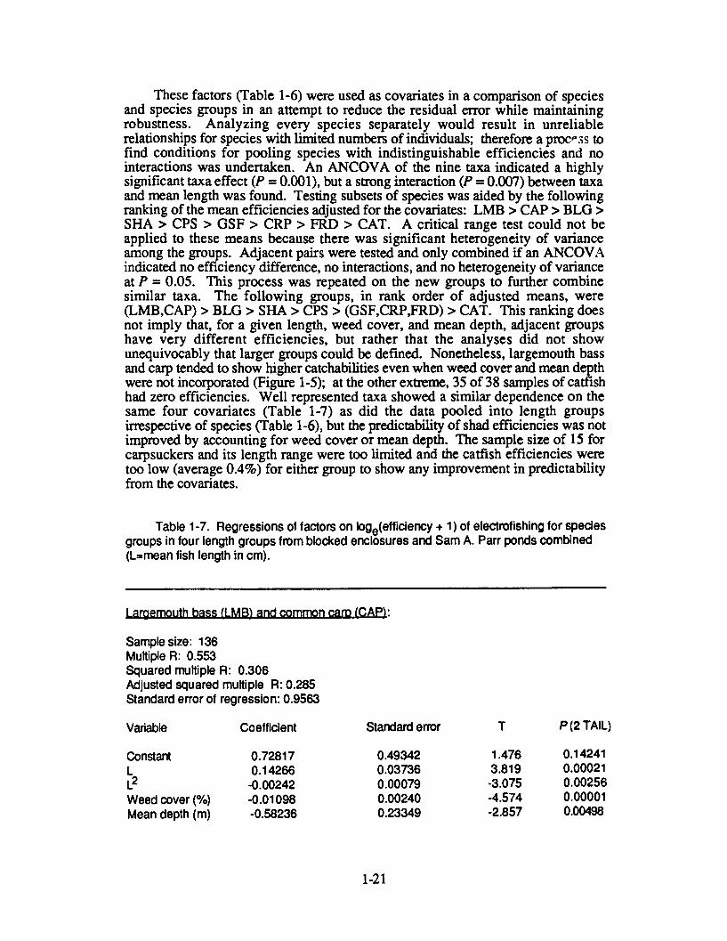
These factors (Table 1-6) were used as covariates in a comparison of speciesand species groups in an attempt to reduce the residual error while maintainingrobustness. Analyzing every species separately would result in unreliablerelationships for species with limited numbers of individuals; therefore a process tofind conditions for pooling species with indistinguishable efficiencies and nointeractions was undertaken. An ANCOVA of the nine taxa indicated a highlysignificant taxa effect (P = 0.001), but a strong interaction (P = 0.007) between taxaand mean length was found. Testing subsets of species was aided by the followingranking of the mean efficiencies adjusted for the covariates: LMB > CAP > BLG >SHA > CPS > GSF > CRP > FRD > CAT. A critical range test could not beapplied to these means because there was significant heterogeneity of varianceamong the groups. Adjacent pairs were tested and only combined if an ANCOVAindicated no efficiency difference, no interactions, and no heterogeneity of varianceat P = 0.05. This process was repeated on the new groups to further combinesimilar taxa. The following groups, in rank order of adjusted means, were(LMB,CAP) > BLG > SHA > CPS > (GSF,CRP,FRD) > CAT. This ranking doesnot imply that, for a given length, weed cover, and mean depth, adjacent groupshave very different efficiencies, but rather that the analyses did not showunequivocably that larger groups could be defined. Nonetheless, largemouth bassand carp tended to show higher catchabilities even when weed cover and mean depthwere not incorporated (Figure 1-5); at the other extreme, 35 of 38 samples of catfishhad zero efficiencies. Well represented taxa showed a similar dependence on thesame four covariates (Table 1-7) as did the data pooled into length groupsirrespective of species (Table 1-6), but the predictability of shad efficiencies was notimproved by accounting for weed cover or mean depth. The sample size of 15 forcarpsuckers and its length range were too limited and the catfish efficiencies weretoo low (average 0.4%) for either group to show any improvement in predictabilityfrom the covariates.
Table 1-7. Regressions of factors on loge(efficiency + 1) of electrofishing for speciesgroups in four length groups from blocked enclosures and Sam A. Parr ponds combined(L=mean fish length in cm).
Largemouth bass (LMB) and common carp (CAP):
Sample size: 136Multiple R: 0.553Squared multiple R: 0.306Adjusted squared multiple R: 0.285Standard error of regression: 0.9563
Variable Coefficient Standard error T P (2 TAIL)
Constant 0.72817 0.49342 1.476 0.14241L 0.14266 0.03736 3.819 0.00021L2 -0.00242 0.00079 -3.075 0.00256Weed cover (%) -0.01098 0.00240 -4.574 0.00001Mean depth (m) -0.58236 0.23349 -2.857 0.00498
1-21
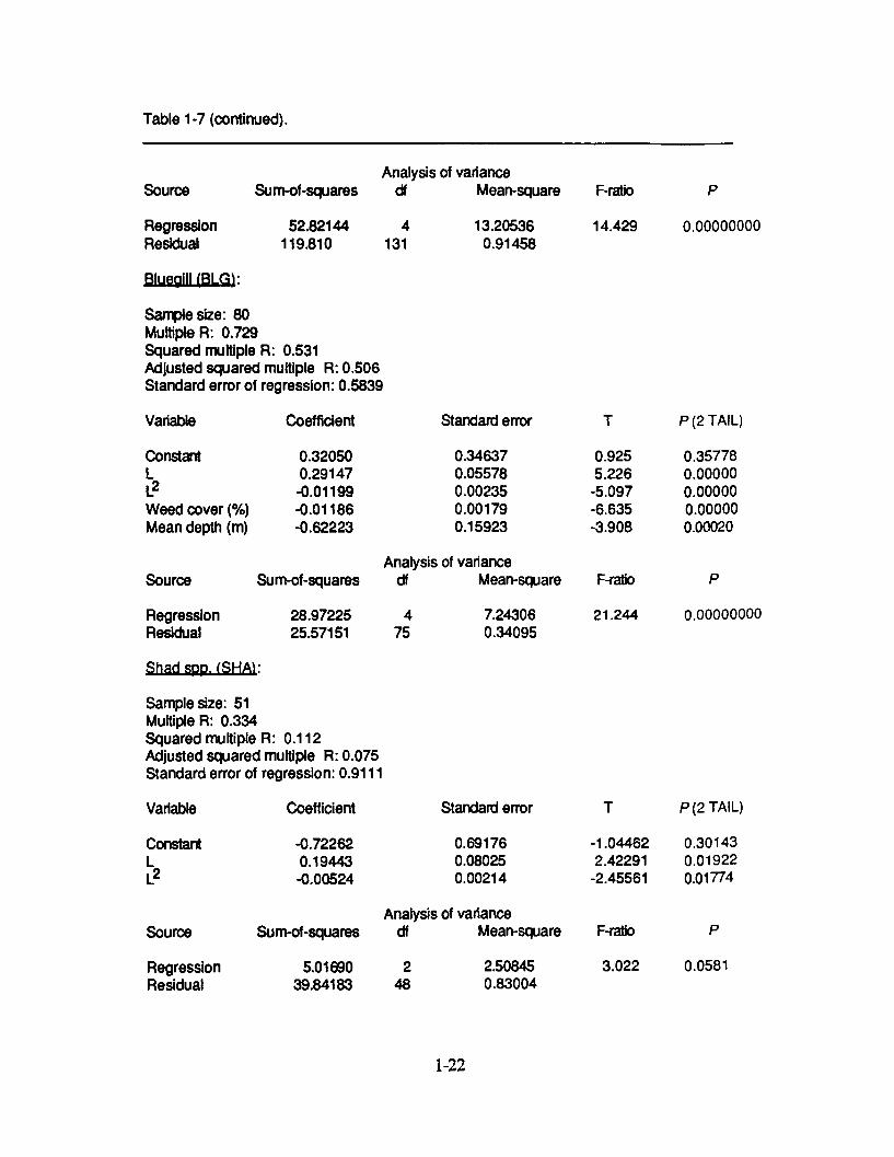
Table 1-7 (continued).
Sum-of-squares
52.82144119.810
Analysis of variancedf Mean-square
4131
Bluegill (BLG):
Sample size: 80Multiple R: 0.729Squared multiple R: 0.531Adjusted squared multiple R: 0.506Standard error of regression: 0.5839
Variable
ConstantLL2Weed cover (%)Mean depth (m)
Source
RegressionResidual
Coefficient
0.320500.29147-0.01199-0.01186-0.62223
Sum-of-squares
28.9722525.57151
Standard error
0.346370.055780.002350.001790.15923
Analysis of variancedf Mean-square
475
7.243060.34095
T
0.9255.226
-5.097-6.635-3.908
F-ratio
21.244
P (2 TAIL)
0.357780.000000.000000.000000.00020
P
0.00000000
Sample size: 51Multiple R: 0.334Squared multiple R: 0.112Adjusted squared multiple R: 0.075Standard error of regression: 0.9111
Coefficient
-0.722620.19443-0.00524
Sum-of-squares
5.0169039.84183
Standard error
0.691760.080250.00214
Analysis of variancedf Mean-square
248
2.508450.83004
1-22
Source
RegressionResidual
13.205360.91458
F-ratio
14.429
P
0.00000000
Variable
ConstantL
Source
RegressionResidual
T
-1.044622.42291
-2.45561
F-ratio
3.022
P (2 TAIL)
0.301430.019220.01774
P
0.0581
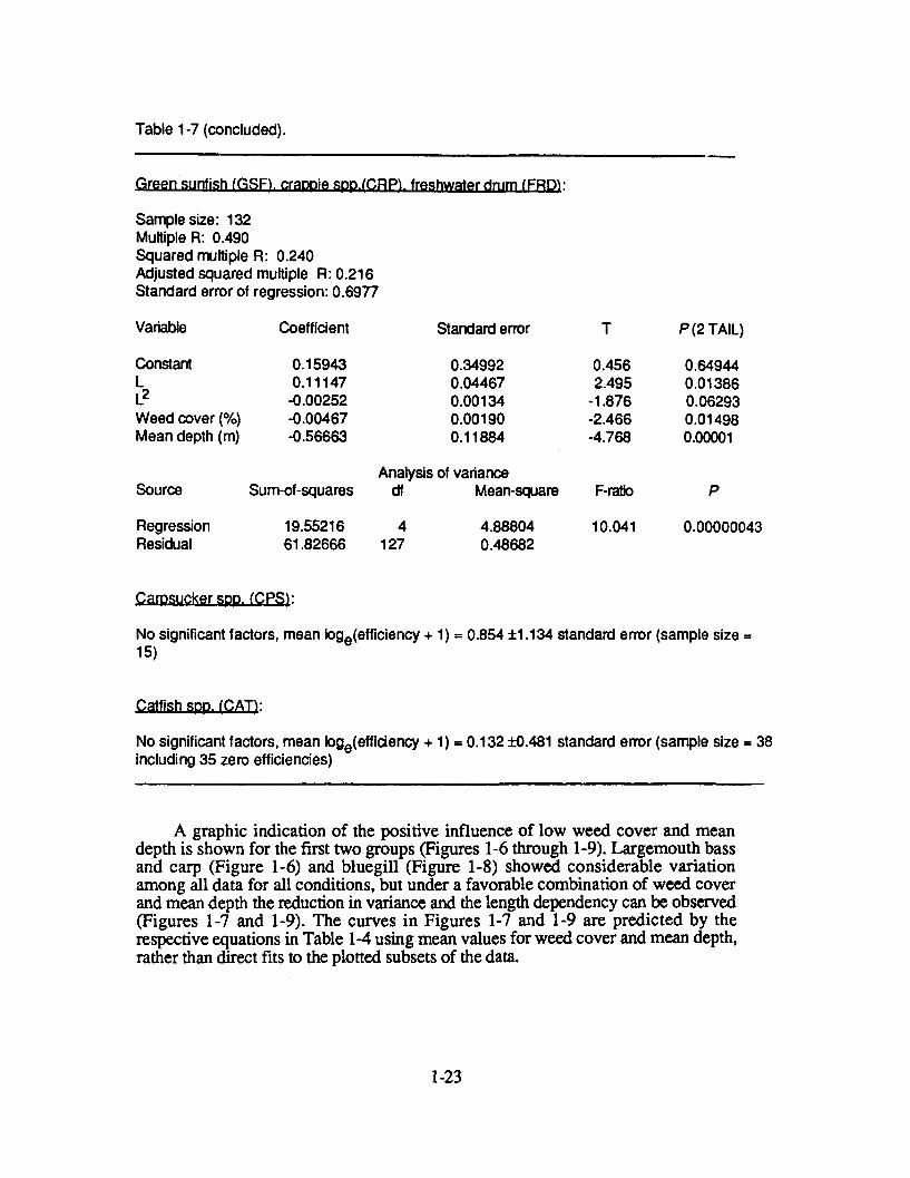
Table 1-7 (concluded).
Green sunfish (GSF). crappie spp.(CRP). freshwater drum (FRD):
Sample size: 132Multiple R: 0.490Squared multiple R: 0.240Adjusted squared multiple R: 0.216Standard error of regression: 0.6977
Variable Coefficient Standard error T P (2 TAIL)
Constant 0.15943 0.34992 0.456 0.64944L 0.11147 0.04467 2.495 0.01386L2 -0.00252 0.00134 -1.876 0.06293Weed cover (%) -0.00467 0.00190 -2.466 0.01498Mean depth (m) -0.56663 0.11884 -4.768 0.00001
Analysis of varianceSource Sum-of-squares df Mean-square F-ratio P
Regression 19.55216 4 4.88804 10.041 0.00000043Residual 61.82666 127 0.48682
Carpsucker spp. (CPS):
No significant factors, mean loge(efficiency + 1) = 0.854 ±1.134 standard error (sample size =15)
Catfish spp. (CAT):
No significant factors, mean loge(efficiency + 1) = 0.132 ±0.481 standard error (sample size = 38including 35 zero efficiencies)
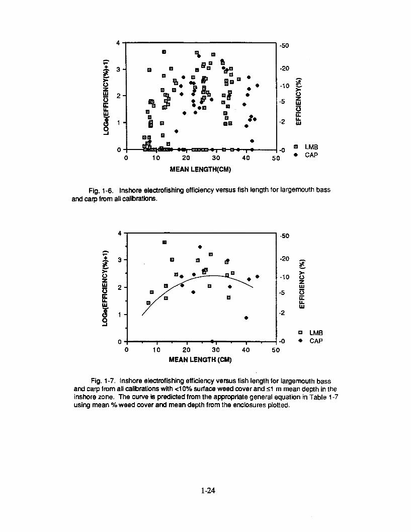
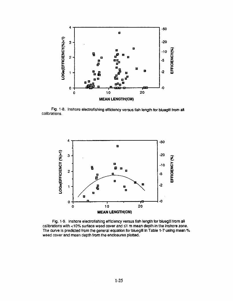
A graphic indication of the positive influence of low weed cover and meandepth is shown for the first two groups (Figures 1-6 through 1-9). Largemouth bassand carp (Figure 1-6) and bluegill (Figure 1-8) showed considerable variationamong all data for all conditions, but under a favorable combination of weed coverand mean depth the reduction in variance and the length dependency can be observed(Figures 1-7 and 1-9). The curves in Figures 1-7 and 1-9 are predicted by therespective equations in Table 1-4 using mean values for weed cover and mean depth,rather than direct fits to the plotted subsets of the data.
1-23
I=
zLUE5VCU.LU
IJ
3-
2-
1-
0 10 20 30 40 50
-50
-20
-10
z-5 mL.
-2 LU
-0
* g m
m B
LMBCAP
MEAN LENGTH(CM)
Fig. 1-6. Inshore electrofishing efficiency versus fish length for largemouth bassand carp from all calibrations.
U
0U Q r
p *U
0 10 20 30MEAN LENGTH (CM)
-50
-20
-10LU
-5 aLLILU
-2
5 LMB-0 * CAP)40 50
Fig. 1-7. Inshore electrofishing efficiency versus fish length for largemouth bassand carp from all calibrations with <10% surface weed cover and _1 m mean depth in theinshore zone. The curve is predicted from the appropriate general equation in Table 1-7using mean % weed cover and mean depth from the enclosures plotted.
1-24
*e, ~ p u*
>p.UozLU
U.
u_
0-J
3
2-
1
B
0
m
I
m AI
w
do
I
÷4.NOR
zLU
LUIL%blo
1
0 1020
20
*
MEAN LENGTH(CM)
Fig. 1-8. Inshore electrofishing efficiency versus fish length for bluegill from allcalibrations.
A
don
z
I.U
w
4.
ILLU
CU.LU
3-
1 -
U
U
U
EBm
lb
0
B
10MEAN LENGTH(CM)
-50
-20 o
-10 C.)
zLU-5 ULI.LU
-2
-020
Fig. 1-9. Inshore electrofishing efficiency versus fish length for bluegill from allcalibrations with <10% surface weed cover and <1 m mean depth in the inshore zone.The curve is predicted from the general equation for bluegill in Table 1-7 using mean %weed cover and mean depth from the enclosures plotted.
1-25
m
1 B3 d- BB
BBB I °!Smm %
* BJF%M M mmBl in 0
m MI .. Mm.
-50
-20
-10
-5
-0
am
i .I s i
w
I
Prediction of Inshore Efficiencies
Although the residual variances are still high, inshore efficiency data are basedon restricted shore lengths (mean = 227 m ± 17 SEM [standard error of the mean])that take only a few minutes to cover (mean = 9.2 min ± 0.8 SEM). Fishing runsand total fishing distance in impoundments are normally much greater than wasphysically possible to simulate in the inshore zone calibrations. Variance ofcatchability decreases as the length of run increases. The residual error from thesmallest enclosures, INHS ponds (shore length = 117 m), was 1.160 comparedwith 0.665 (Table 1-6) for the intermediate enclosures and large ponds used in theinshore zone analysis (mean shore length 227 m). A residual error of 0.433 from adifferent multiple regression from the five large lake samples was still lower, despitethe additional complications of inshore/offshore distribution of fish, the variation inhabitat, and the limited number of samples. Errors of the mean inshore catchabilityduring the more typical, longer runs used in impoundment surveys were estimatedfor key species in Table 1-8 according to the central limit theory, that in effectassumes a run is equivalent to an independent series of inshore calibration runs. A1,550-m run lasting about 60 min is equivalent to about seven inshore calibrationruns.
The implications of Table 1-5 are described by numerical examples. Supposethat ten largemouth bass and ten bluegill in the third (mean = 25 cm) and second(mean = 15 cm) length groups, respectively, were caught under the more favorableconditions of no weed cover and a mean depth of 0.5 m within the inshore zoneduring a 1,550-m (5,085-ft) sample taking about 60 min. The estimated abundancesare 100 LMB and 240 BLG individuals, with respective 95% confidence ranges of42-210 and 140-410. The lower and upper limits are, respectively, 0.47 and 2.3times the LMB mean abundance and 0.61 and 1.8 times the BLG mean abundance.If the impoundment was large enough to allow six times the sampling effort, theupper and lower limits would be, respectively, 0.73 and 1.4 times the LMB meanabundance and 0.78 and 1.26 times the BLG abundance--a considerableimprovement at the cost of increased sampling effort. These estimates do not takeinto account the sampling variance due to spatial heterogeneity of fish distributionthat would be an additional factor if the entire shoreline were not sampled.
Under more difficult sampling conditions of 50% weed cover and 1.5 m meandepth in the inshore zone, the residual errors of the transformed efficiencies aresimilar because of the very small errors of these predictors (Table 1-7), but the lowermean efficiencies result in wider confidence intervals of the untransformedefficiencies. In the LMB example, the mean efficiency is 3.8 times lower than thatunder the more favorable conditions. This reduction was related to wider lower andupper confidence limits that were, respectively, 0.41 and 3.3 times the LMB meanabundance for a 1,550-m sample. With BLG, mean efficiency is 7.3 times lower,but, more importantly, there is an extremely wide confidence interval for a 1,550-msample (Table 1-8). Under worse conditions, or with slightly larger bluegill, theefficiency confidence range would include zero from a 1,550-m (60-min) sample.This implies that no realistic estimate of abundance could be made from such asample and that a large sampling effort would be required to detect moderatedifferences in population densities from year to year.
1-26
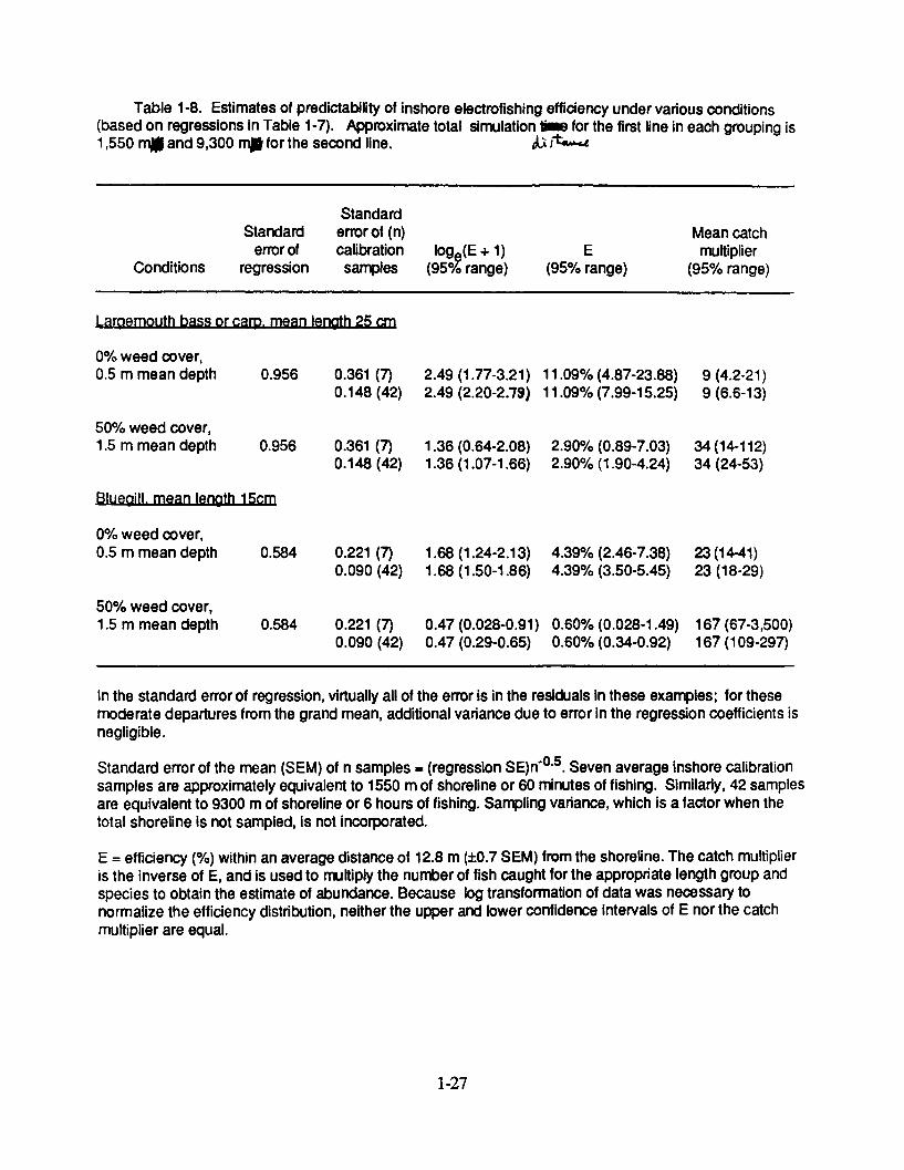
Table 1-8. Estimates of predictability of inshore electrofishing efficiency under various conditions(based on regressions in Table 1-7). Approximate total simulation im for the first line in each grouping is1,550 mno and 9,300 mI for the second line. A J1
StandardStandard error of (n) Mean catch
error of calibration loge(E + 1) E multiplierConditions regression samples (95% range) (95% range) (95% range)
Largemouth bass or carp. mean length 25 cm
0% weed cover,0.5 m mean depth 0.956 0.361 (7) 2.49 (1.77-3.21) 11.09% (4.87-23.88) 9 (4.2-21)
0.148 (42) 2.49 (2.20-2.79) 11.09% (7.99-15.25) 9 (6.6-13)
50% weed cover,1.5 m mean depth 0.956 0.361 (7) 1.36 (0.64-2.08) 2.90% (0.89-7.03) 34 (14-112)
0.148 (42) 1.36 (1.07-1.66) 2.90% (1.90-4.24) 34 (24-53)
Blueaill. mean length 15cm
0% weed cover,0.5 m mean depth 0.584 0.221 (7) 1.68 (1.24-2.13) 4.39% (2.46-7.38) 23 (14-41)
0.090 (42) 1.68 (1.50-1.86) 4.39% (3.50-5.45) 23 (18-29)
50% weed cover,1.5 m mean depth 0.584 0.221 (7) 0.47 (0.028-0.91) 0.60% (0.028-1.49) 167 (67-3,500)
0.090 (42) 0.47 (0.29-0.65) 0.60% (0.34-0.92) 167 (109-297)
In the standard error of regression, virtually all of the error is in the residuals in these examples; for thesemoderate departures from the grand mean, additional variance due to error in the regression coefficients isnegligible.
Standard error of the mean (SEM) of n samples = (regression SE)n0"°5 . Seven average inshore calibrationsamples are approximately equivalent to 1550 m of shoreline or 60 minutes of fishing. Similarly, 42 samplesare equivalent to 9300 m of shoreline or 6 hours of fishing. Sampling variance, which is a factor when thetotal shoreline is not sampled, is not incorporated.
E = efficiency (%) within an average distance of 12.8 m (±0.7 SEM) from the shoreline. The catch multiplieris the inverse of E, and is used to multiply the number of fish caught for the appropriate length group andspecies to obtain the estimate of abundance. Because log transformation of data was necessary tonormalize the efficiency distribution, neither the upper and lower confidence intervals of E nor the catchmultiplier are equal.
1-27
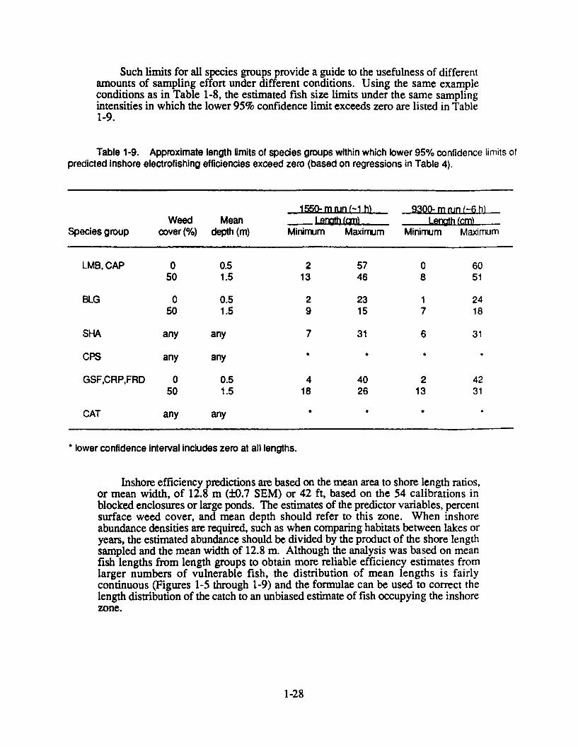
Such limits for all species groups provide a guide to the usefulness of differentamounts of sampling effort under different conditions. Using the same exampleconditions as in Table 1-8, the estimated fish size limits under the same samplingintensities in which the lower 95% confidence limit exceeds zero are listed in Table1-9.
Table 1-9. Approximate length limits of species groups within which lower 95% confidence limits ofpredicted inshore electrofishing efficiencies exceed zero (based on regressions in Table 4).
1550- m run (--1 h) 9300- mrun (-6 h)Weed Mean Length (cm) Length (cm)
Species group cover (%) depth (m) Minimum Maximum Minimum Maximum
LMB, CAP 0 0.5 2 57 0 6050 1.5 13 46 8 51
BLG 0 0.5 2 23 1 2450 1.5 9 15 7 18
SHA any any 7 31 6 31
CPS any any * * *
GSF,CRP,FRD 0 0.5 4 40 2 4250 1.5 18 26 13 31
CAT any any * * * *
* lower confidence interval includes zero at all lengths.
Inshore efficiency predictions are based on the mean area to shore length ratios,or mean width, of 12.8 m (±0.7 SEM) or 42 ft, based on the 54 calibrations inblocked enclosures or large ponds. The estimates of the predictor variables, percentsurface weed cover, and mean depth should refer to this zone. When inshoreabundance densities are required, such as when comparing habitats between lakes oryears, the estimated abundance should be divided by the product of the shore lengthsampled and the mean width of 12.8 m. Although the analysis was based on meanfish lengths from length groups to obtain more reliable efficiency estimates fromlarger numbers of vulnerable fish, the distribution of mean lengths is fairlycontinuous (Figures 1-5 through 1-9) and the formulae can be used to correct thelength distribution of the catch to an unbiased estimate of fish occupying the inshorezone.
1-28
Comparisons between Inshore and Large Water-body Efficiencies
Efficiency estimates from key species caught in the five large water-bodycalibrations (Table 1-4) were compared with the inshore calibration results todiscover if the inshore calibrations can be used to estimate the fish population in alarge water body. In other words, is part of the fish population outside the inshorezone?
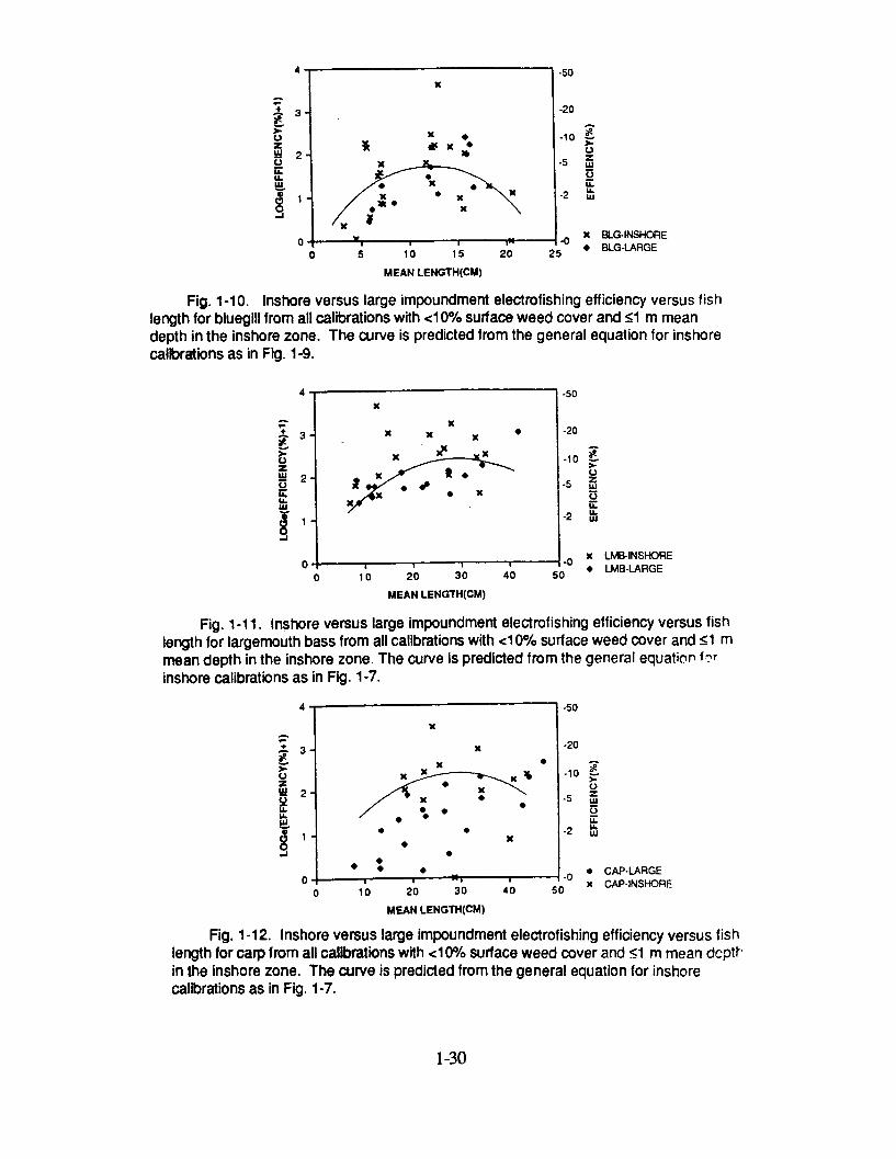
All large water-body samples were taken under favorable conditions of lowweed cover and shallow mean depths in the inshore zone. Therefore, the inshoreefficiency data corresponding to these conditions (e.g., Figures 1-7 and 1-9) werecompared with those from whole water body studies (Figures 1-10 through 1-12).ANCOVA comparisons for bluegill and largemouth bass (Figures 1-10 and 1-11)indicated that the whole water-body efficiencies were not significantly different fromthe inshore data. Therefore, predictions from inshore catch per unit effort for thesespecies under these conditions can be made for whole populations. However, thewhole water-body efficiencies for carp (Figure 1-12) were significantly (P < 0.05)lower than the inshore efficiencies (the difference being more significant (P < 0.01)for fish <40 cm long). This indicates that significant quantities of carp wereoffshore and not vulnerable to the electroshocker.
Discussion
There are limited data that can be compared to this study. Simpson (1978)sampled 13 coves and 10 ponds with an AC boat electroshocker fished at night andcollected efficiency data taken with varying methods by other workers.Unfortunately, his statistical analysis was inadequate (multiple testing of selectedpairs of variables without testing for correlations or interactions between them), therotenone efficiencies were presumed to be 100%, and the precision of estimatedefficiencies was not analyzed.
Our analyses determine the variance of efficiency estimates but do not accountfor sampling variance of catch data from a series of samples. Currently, there areinadequate data to pursue this further, but we believe that, with properly designedsurveys, sampling variance of the boat electroshocker will prove to be minorcompared with the catchability variance (see General Discussion). There is noassurance, however, that abundance density can be inferred from smallimpoundments with acceptable accuracy from CPUE data even if the wholeshoreline can be sampled, unless it is resampled repeatedly with time intervalsbetween samples to permit fish recovery. 'Acceptable accuracy' is a managementdecision. For example, it may be considered desirable for sampling effort to besufficient to detect a 25% change in a largemouth bass population with 95%confidence from one year to the next. The examples in Tables 1-8 and 1-9 indicatethat the quantity of sampling is important. Even the presence or absence of somespecies and sizes cannot be reliably determined; for example, sampling the entire750-m shoreline of a 4.5-ha (11-acre) pond, taking about 30 min, could fail tocapture catfish, freshwater drum, crappies, or green sunfish.
It was impossible to evaluate all extreme values of conditions that may affectcatchability. However, most extreme values, such as very clear or turbid water, lowconductivity, or deep water that are beyond the values encountered in this study, can
1-29
I I I I~.
0 5 10 15 20 25
-50
-20
-10
-5
-2 u
x BLG-INSHORE,a B LG-If ARGC-
MEAN LENGTH(CM)
Fig. 1-10. Inshore versus large impoundment electrofishing efficiency versus fishlength for bluegill from all calibrations with <10% surface weed cover and <1 m meandepth in the inshore zone. The curve is predicted from the general equation for inshorecalibrations as in Fig. 1-9.
0 10 20 30
-50
-20
-10z
-5 J
-2 mU
x LMB-INSHORE-0 0 LMBJ-LARGE-40 50MEAN LENGTH(CM)
Fig. 1-11. Inshore versus large impoundment electrofishing efficiency versus fishlength for largemouth bass from all calibrations with <10% surface weed cover and <1 mmean depth in the inshore zone. The curve is predicted from the general equation flrinshore calibrations as in Fig. 1-7.
-50
-20
-10
z
-2
-0 CAP-LARGEx CAP-INSHORE
MEAN LENGTH(CM)
Fig. 1-12. Inshore versus large impoundment electrofishing efficiency versus fishlength for carp from all calibrations with <10% surface weed cover and <1 m mean depthin the inshore zone. The curve is predicted from the general equation for inshorecalibrations as in Fig. 1-7.
1-30
+ 3-3-
z. 2
uL
0
x
XXx
* x*xx
x x9 K
0--+
UJzLUU.
LL
LL
LU
3 -
2-
1
K
K
K K
K ciC K
KK 9 K
K
Uzw
5.wu_&a
JB.
I !-I -0I I I I
domftV-46Tp
w
be expected to result in lower efficiency. Because it is unlikely that this reductionwould be ameliorated by a lower variance of efficiency, such extreme conditions willlimit our ability to make inferences about fish populations from a given samplingeffort. Even from the crude viewpoint of fish catches from a range of gears it isevident that electrofishing the low conductivity, clear-water impoundments oftenfound in Southern Illinois or the deep, clear waters typical of strip-mining ponds,for example, cannot produce reliable inferences about fish population densities.
The effects of mean depth and weed cover on inshore efficiency may not beentirely independent. In practice, when weed cover becomes dense, the boat isdirected farther offshore. This was simulated in the calibration experiments, inwhich mean depth and weed cover were uncorrelated. Efficiency may be reduced bythe effect of increased depth at the boat position as well as by missing fish in theweed beds due to lack of proximity or inability to find stunned fish.
The typical association between weeds and water clarity was evident in acorrelation between weed cover and secchi disk, and these variables were keptseparate in multivariate analyses. Except for extremely turbid waters, one wouldexpect efficiency to decrease with increasing water clarity (e.g., Simpson 1978),producing a negative coefficient. However, when weed cover was substituted bysecchi value as a factor, the latter was not significant and its coefficient was positiveeven though the secchi disk range in the inshore calibrations was 18-173 cm. Also,in a subset of data of <10% weed cover, the secchi disk factor was not significant.However, the negative effect of weed cover could have been enhanced by increasedwater clarity when weed cover increased. Sampling in extremely clear waterprobably does have a negative effect on efficiency by scaring fish, which counteractsthe positive effect of easier observation for capture. But clear water is typicallyassociated with deep or low conductivity waters in which the low efficiency is soself-evident that calibration would not be worthwhile. The calibrations completedinclude ranges and combinations of conditions typical of most Illinoisimpoundments where some level of quantitative inference from boat electrofishingdata is possible.
It is therefore important during regular surveys to not only record informationof factors that were found to be significant in this study. Other factors may beoutside the range encountered, particularly secchi disk and conductivity (or alkalinityas a proxy). Because sampling sites are fixed, mean depth in the inshore zone isfairly constant and is being measured for all permanent sites in project F-69-R.However, surface weed cover can vary significantly between years at the same siteand season.
This study is not restricted to the inference of population density, but alsoapplies to population structure. The effect of length is apparent in all taxa that arerepresented by a sufficient length range and quantity of calibration samples.Unbiased population structure estimates are required for calculations of mortality andsuch static, structural indices as PSD. The alternative to using the efficiencyformulae to correct the length frequency and obtain an unbiased PSD estimate wouldbe to define a 'boat electrofishing PSD.' Although many PSD estimates in theliterature are implicitly based on the latter definition there are problems that gobeyond the obvious one of gear conformity.
1-31
If a PSD estimate was derived from pooled samples where, for example, thesmaller fish were obtained in areas with high weed cover and the larger ones fromweed-free water, 'boat electrofishing PSD' would overestimate the PSD of thepopulation. Conversely, if the samples were characterized by weed cover and wereindividually corrected for efficiency and weighted by shore length before pooling, anunbiased PSD could be estimated. The first condition, sample characterization, isimportant; data from a few, very long electrofishing runs (samples) covering avariety of conditions that affect efficiency cannot be guaranteed to provide unbiasedestimates of PSD even if an efficiency correction is applied based on averageconditions. This problem cannot be entirely avoided, but many, shorterelectrofishing samples will reduce the bias. Similar scenarios can be envisaged forinferences of population density.
What about DC electrofishing? Will it provide a significant increase inefficiency without an equivalent increase in variance? Very limited efficiency dataare available. D. Foster (cited in Simpson 1978) found that for 0.5-acre ponds meanefficiencies of largemouth bass increase from 13.3% with AC to 19.1% with DCand those of bluegill increase from 3.8% with AC to 5.8% with DC. Unless therewas also a marked improvement in efficiency variance, these increases would notsubstantially improve the predictability of population density. We suspect that a DCrig can be designed and tuned to increase the efficiency of almost any species andsize combination by optimizing the settings for galvanotaxis under givenenvironmental conditions. But a common misconception is that all captures using aDC rig under constant settings are due to galvanotaxis, whereas a large proportionare caught by galvanonarcosis as with AC current. The effect of AC, however, isstronger and can occasionally produce tetany. A correctly tuned DC rig is efficientfor catching a target species within a defined length range, and given sufficientvoltage and power, is reputed to catch more fish in lower conductivity water that ACunits.
Apart from high cost and power requirements, there are two problems with DCunits associated with its complexity. First, there are more things to go wrong.Second, the tendency of most field biologists is to try to optimize the catch accordingto their concept of the sampling conditions and the fish of interest. Such anon-standard fishing approach would be as impractical to calibrate as an individualangler with a box full of lures and baits, even if the numerous combinations ofvoltage, pulse width, and pulse frequency were recorded. In principal, theseproblems can be overcome; given the limitations of AC electrofishing and other gearpresented here, a DC unit should be investigated for use in environments where anAC unit is only marginally useful.
GILLNET EFFICIENCIES
Methods
A standard gillnet fleet used by IDOC was fished in enclosures ranging from0.15 to 5.565 ha (0.4-13.8 acres) in which vulnerable fish population wereestimated from rotenone or draining. The standard gillnet fleet is 125 ft long with 5panels of 1.5-, 2-, 3-, 4-, and 5-in. stretched mesh. Additional data were collectedin 1983 using a similar fleet that was 125 ft long but had 6 panels of 1-, 2-, 2.5-, 3-,
1-32
4-, and 5-in. stretched mesh. Conditions for 37 calibrated gillnet samples are listedin Table 1-10.
Small enclosures were generally avoided because the gear is not normally iusedin ponds. However, variation in enclosure area is important because its influence oncatchability needs to be assessed; i.e., does a standard fleet catch the sameproportion of fish from a 0.5-ha impoundment as it does from a 5-ha one? Gillnetswere fished prior to any electrofishing calibration. Before contiguous enclosureswere constructed in coves for electrofishing, the entire cove was blocked by a singlenet for gillnet sets. Likewise, a large impoundment was fished with standard fleetsbefore enclosures were created along parts of the shoreline for electrofishingcalibrations. When fleets were fished on successive days in the same enclosure, theirlocations were changed. No general trend in decreasing or increasing catch wasobserved. Two fleets were fished in different halves of the largest enclosures (22.7ha).
Gillnet efficiency studies typically estimate the relative efficiency of adjacentpairs of mesh sizes. Relative efficiency can correct length frequency distributionsfor the modes representing maximum catchability for each mesh, so that modespresent in the vulnerable population, such as those representing age cohorts, can beidentified. However, it assumes that each mesh has the same absolute catchabilityand provides no information on fish abundance except in the form of an index. Thisstudy regards the whole fleet as a single unit, which corresponds to the IDOCapproach because they do not measure fish from each mesh separately (we didmeasure fish from each mesh separately for future analyses). Efficiency is definedas the proportion of vulnerable fish caught by one unit of the fleet during a 24-h set.The fleet was set on the bottom with the small mesh end attached to the shore; thelarge mesh end was anchored offshore at an angle to shore of 45-90°. This methodparallels the most common IDOC approach.
Data Analysis and Results
A similar process to that developed for the inshore electrofishing calibrations,i.e., four length groups and use of the transformation logo(efficiency(%) + 1),removed the skew in the error distribution and helped to stabilize the variability. Allfish irrespective of species and individual taxa were analyzed, as was done withelectrofishing calibrations. Estimates based on fewer than 5 recovered fish wereexcluded.
A variety of uncorrelated factors that might possibly affect catchability: fishlength, enclosure area, secchi disk reading, temperature, and mean depth were usedin an attempt to explain the variance of the tranformed efficiency estimates. With allfish combined, fish length and fish length squared were significant factors at P =0.00006 and P = 0.017, respectively, but no other factor was remotely significant.The parabolic relationship with fish length explained only 33% of the variance intransformed efficiency, with smaller and very large fish showing lower efficiencies.The corresponding standard error of regression, 0.320, however, was smaller thanthose for inshore electrofishing calibrations (Table 1-6).
1-33
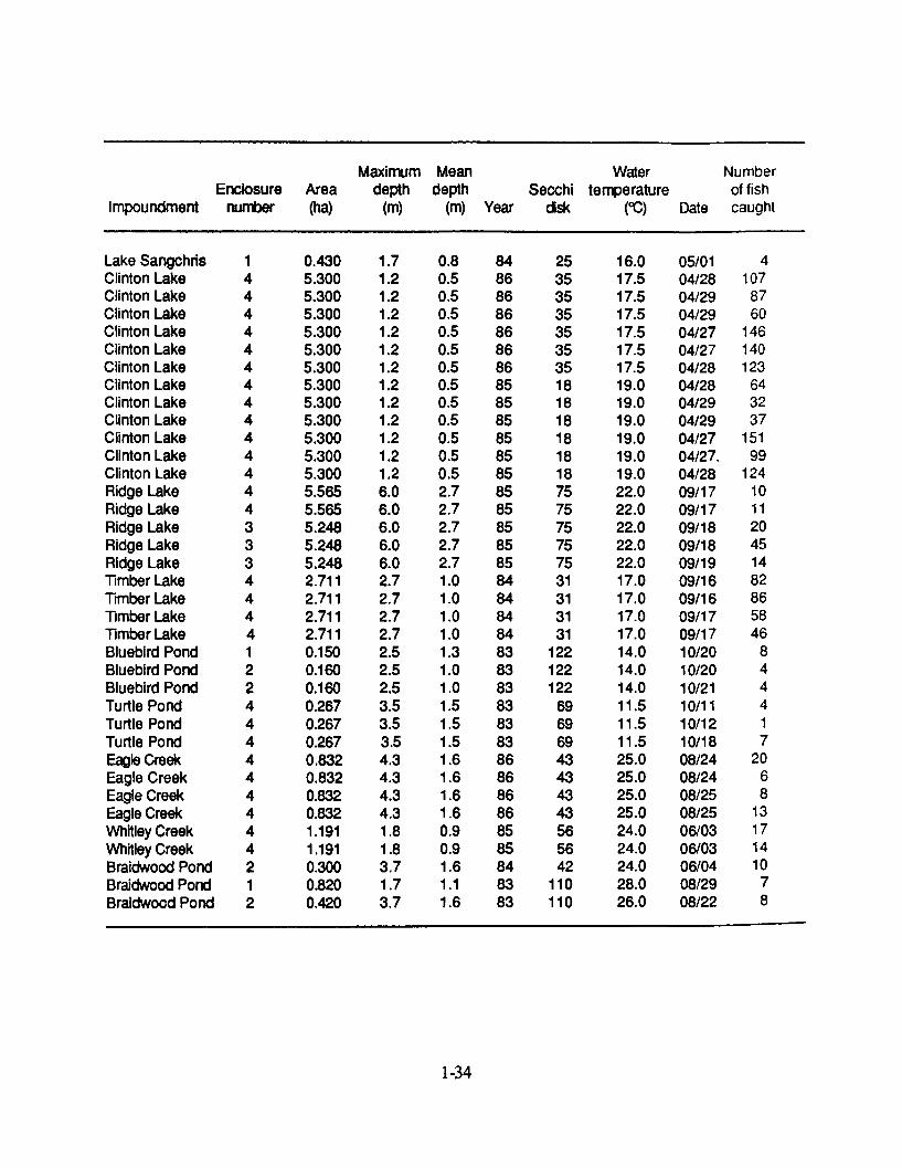
Maximum Mean Water NumberEnclosure Area depth depth Secchi temperature of fish
Impoundment number (ha) (m) (m) Year disk (CC) Date caught
Lake SangchrisClinton LakeClinton LakeClinton LakeClinton LakeClinton LakeClinton LakeClinton LakeClinton LakeClinton LakeClinton LakeClinton LakeClinton LakeRidge LakeRidge LakeRidge LakeRidge LakeRidge LakeTimber LakeTimber LakeTimber LakeTimber LakeBluebird PondBluebird PondBluebird PondTurtle PondTurtle PondTurtle PondEagle CreekEagle CreekEagle CreekEagle CreekWhitley CreekWhitley CreekBraidwood PondBraidwood PondBraidwood Pond
1444444444444443334444122444444444212
0.4305.3005.3005.3005.3005.3005.3005.3005.3005.3005.3005.3005.3005.5655.5655.2485.2485.2482.7112.7112.7112.7110.1500.1600.1600.2670.2670.2670.8320.8320.8320.8321.1911.1910.3000.8200.420
1.71.21.21.21.21.21.21.21.21.21.21.21.26.06.06.06.06.02.72.72.72.72.52.52.53.53.53.54.34.34.34.31.81.83.71.73.7
0.80.50.50.50.50.50.50.50.50.50.50.50.52.72.72.72.72.71.01.01.01.01.31.01.01.51.51.51.61.61.61.60.90.91.61.11.6
84868686868686858585858585858585858584848484838383838383868686868585848383
25353535353535181818181818757575757531313131
12212212269696943434343565642
110110
16.0 05/0117.5 04/2817.5 04/2917.5 04/2917.5 04/2717.5 04/2717.5 04/2819.0 04/2819.0 04/2919.0 04/2919.0 04/2719.0 04/27.19.0 04/2822.0 09/1722.0 09/1722.0 09/1822.0 09/1822.0 09/1917.0 09/1617.0 09/1617.0 09/1717.0 09/1714.0 10/2014.0 10/2014.0 10/2111.5 10/1111.5 10/1211.5 10/1825.0 08/2425.0 08/2425.0 08/2525.0 08/2524.0 06/0324.0 06/0324.0 06/0428.0 08/2926.0 08/22
1-34
41078760
146140123643237
15199
124101120451482865846
84441720
681317141078
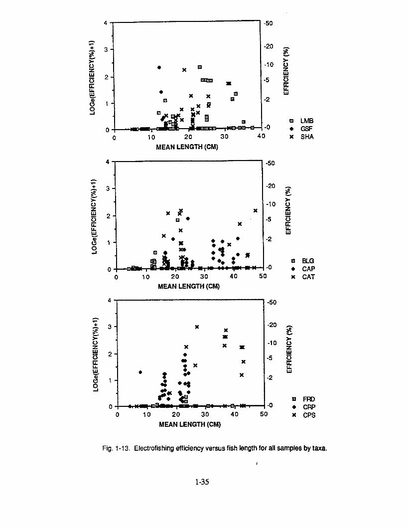
4
0 10 20 30
MEAN LENGTH (CM)
0 10 20 30
MEAN LENGTH (CM)
0 10 20 30
MEAN LENGTH (CM)
3
1 -
0
0
U-"
LU
4.z
03i
1 40 x SHA
-50
-20 o
-10zLU
-5 0
LJ-2
m BLG-0 * CAP
40 50 x CAT
40
-50
-nt-rV
-10 Uz-5 i
-2
-0 *Xx
FRDCRPCPS5
Fig. 1-13. Electrofishing efficiency versus fish length for all samples by taxa.
1-35
0 0z
LU
a LMB* GSF
3
2
+
0-
>-
zLU
U.LU
0.j0
4
A
*0town
zLUC
LU
U)o
0.i
x
x x x
* x* x
/? $°
- *q -
m
an -J m
)
*
50
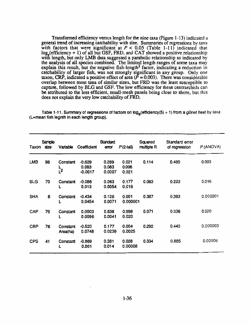
Transformed efficiency versus length for the nine taxa (Figure 1-13) indicated ageneral trend of increasing catchability with size. Summaries of regressions by taxawith factors that were significant at P < 0.05 (Table 1-11) indicated thatlog (efficiency + 1) of all but GSF, FRD, and CAT showed a positive relationshipwith length, but only LMB data suggested a parabolic relationship as indicated bythe analysis of all species combined. The limited length ranges of some taxa mayexplain this result, but the negative fish-length2 factor, indicating a reduction incatchability of larger fish, was not strongly significant in any group. Only onetaxon, CRP, indicated a positive effect of area (P = 0.003). There was considerableoverlap between most taxa of similar sizes, but FRD was the least susceptible tocapture, followed by BLG and GSF. The low efficiency for these centrarchids canbe attributed to the less efficient, small-mesh panels being close to shore, but thisdoes not explain the very low catchability of FRD.
Table 1-11. Summary of regressions of factors on loge(efficiency(5) + 1) from a gillnet fleet by taxa(L=mean fish legnth in each length group).
Sample Standard Squared Standard errorTaxon size Variable Coefficient error P(2-tail) multiple R of regression P (ANOVA)
LMB 98 Constant -0.629 0.269 0.021 0.114 0.480 0.003L 0.083 0.083 0.006L2 -0.0017 0.0007 0.021
BLG 70 Constant -0.086 0.063 0.177 0.083 0.223 0.016L 0.013 0.0054 0.016
SHA 6 Constant -0.434 0.126 0.001 0.387 0.383 0.000001L 0.0454 0.0071 0.000001
CAP 76 Constant 0.0003 0.638 0.998 0.071 0.336 0.020L 0.0096 0.0041 0.020
CRP 76 Constant -0.520 0.177 0.004 0.292 0.440 0.000003Area(ha) 0.0748 0.0239 0.0025
CPS 41 Constant -0.869 0.381 0.028 0.334 0.885 0.00008L 0.061 0.014 0.00008
1-36
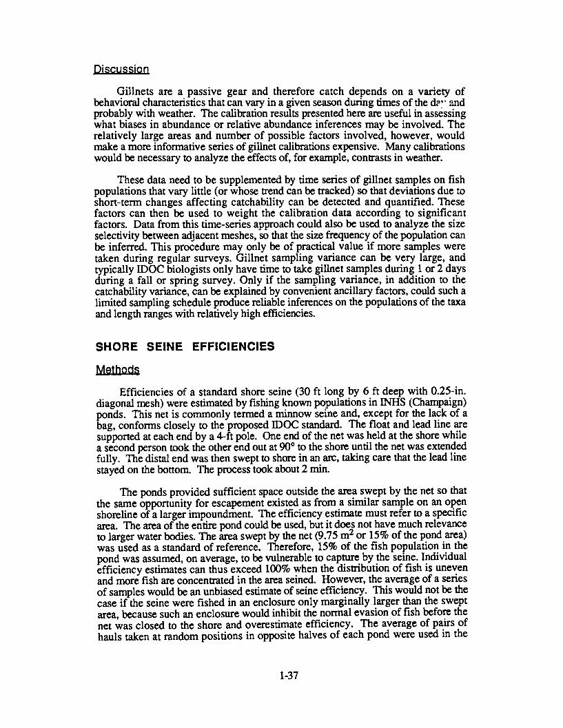
Discussion
Gillnets are a passive gear and therefore catch depends on a variety ofbehavioral characteristics that can vary in a given season during times of the d'r" andprobably with weather. The calibration results presented here are useful in assessingwhat biases in abundance or relative abundance inferences may be involved. Therelatively large areas and number of possible factors involved, however, wouldmake a more informative series of gillnet calibrations expensive. Many calibrationswould be necessary to analyze the effects of, for example, contrasts in weather.
These data need to be supplemented by time series of gillnet samples on fishpopulations that vary little (or whose trend can be tracked) so that deviations due toshort-term changes affecting catchability can be detected and quantified. Thesefactors can then be used to weight the calibration data according to significantfactors. Data from this time-series approach could also be used to analyze the sizeselectivity between adjacent meshes, so that the size frequency of the population canbe inferred. This procedure may only be of practical value if more samples weretaken during regular surveys. Gillnet sampling variance can be very large, andtypically IDOC biologists only have time to take gillnet samples during 1 or 2 daysduring a fall or spring survey. Only if the sampling variance, in addition to thecatchability variance, can be explained by convenient ancillary factors, could such alimited sampling schedule produce reliable inferences on the populations of the taxaand length ranges with relatively high efficiencies.
SHORE SEINE EFFICIENCIES
Methods
Efficiencies of a standard shore seine (30 ft long by 6 ft deep with 0.25-in.diagonal mesh) were estimated by fishing known populations in INHS (Champaign)ponds. This net is commonly termed a minnow seine and, except for the lack of abag, conforms closely to the proposed IDOC standard. The float and lead line aresupported at each end by a 4-ft pole. One end of the net was held at the shore whilea second person took the other end out at 90° to the shore until the net was extendedfully. The distal end was then swept to shore in an arc, taking care that the lead linestayed on the bottom. The process took about 2 min.
The ponds provided sufficient space outside the area swept by the net so thatthe same opportunity for escapement existed as from a similar sample on an openshoreline of a larger impoundment. The efficiency estimate must refer to a specificarea. The area of the entire pond could be used, but it does not have much relevanceto larger water bodies. The area swept by the net (9.75 m2 or 15% of the pond area)was used as a standard of reference. Therefore, 15% of the fish population in thepond was assumed, on average, to be vulnerable to capture by the seine. Individualefficiency estimates can thus exceed 100% when the distribution of fish is unevenand more fish are concentrated in the area seined. However, the average of a seriesof samples would be an unbiased estimate of seine efficiency. This would not be thecase if the seine were fished in an enclosure only marginally larger than the sweptarea, because such an enclosure would inhibit the normal evasion of fish before thenet was closed to the shore and overestimate efficiency. The average of pairs ofhauls taken at random positions in opposite halves of each pond were used in the
1-37
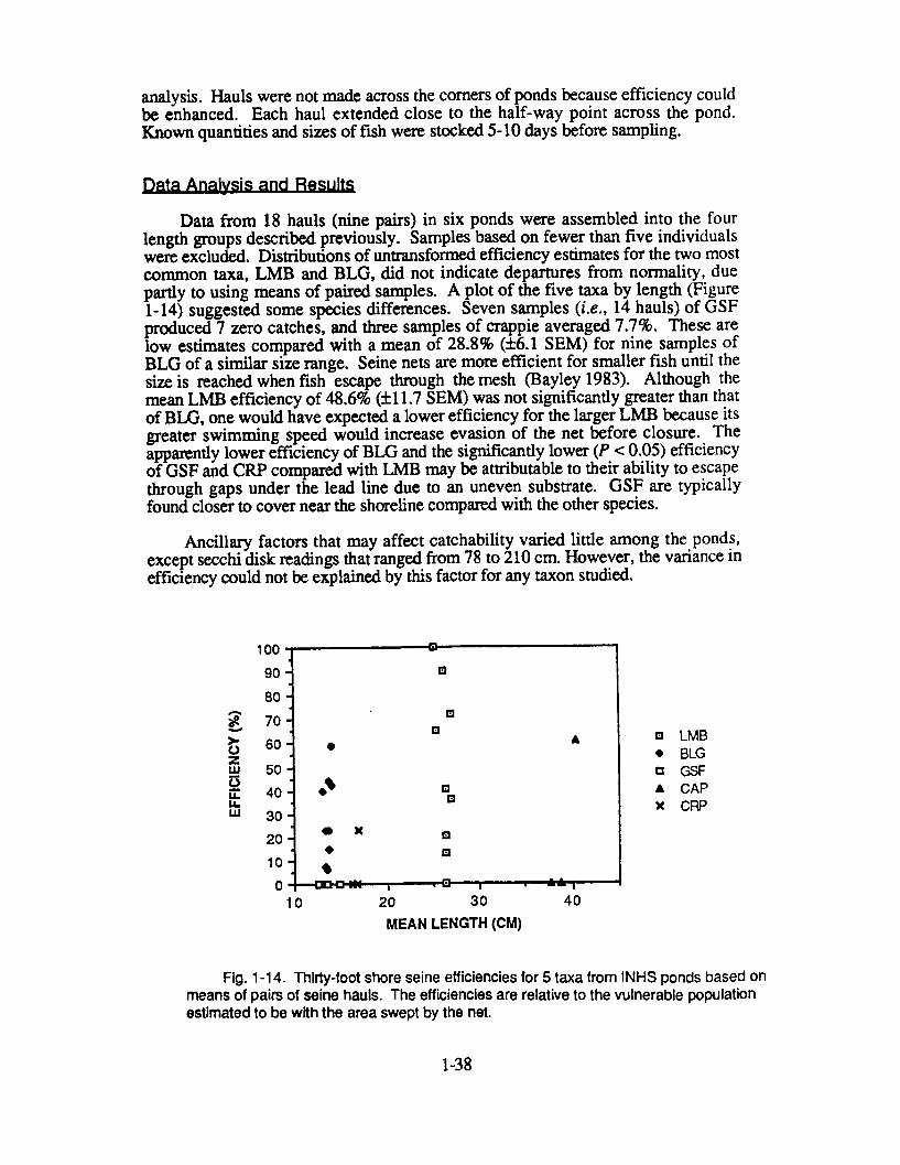
analysis. Hauls were not made across the comers of ponds because efficiency couldbe enhanced. Each haul extended close to the half-way point across the pond.Known quantities and sizes of fish were stocked 5-10 days before sampling.
Data Analysis and Results
Data from 18 hauls (nine pairs) in six ponds were assembled into the fourlength groups described previously. Samples based on fewer than five individualswere excluded. Distributions of untransformed efficiency estimates for the two mostcommon taxa, LMB and BLG, did not indicate departures from normality, duepartly to using means of paired samples. A plot of the five taxa by length (Figure1-14) suggested some species differences. Seven samples (i.e., 14 hauls) of GSFproduced 7 zero catches, and three samples of crappie averaged 7.7%. These arelow estimates compared with a mean of 28.8% (±6.1 SEM) for nine samples ofBLG of a similar size range. Seine nets are more efficient for smaller fish until thesize is reached when fish escape through the mesh (Bayley 1983). Although themean LMB efficiency of 48.6% (±11.7 SEM) was not significantly greater than thatof BLG, one would have expected a lower efficiency for the larger LMB because itsgreater swimming speed would increase evasion of the net before closure. Theapparently lower efficiency of BLG and the significantly lower (P < 0.05) efficiencyof GSF and CRP compared with LMB may be attributable to their ability to escapethrough gaps under the lead line due to an uneven substrate. GSF are typicallyfound closer to cover near the shoreline compared with the other species.
Ancillary factors that may affect catchability varied little among the ponds,except secchi disk readings that ranged from 78 to 210 cm. However, the variance inefficiency could not be explained by this factor for any taxon studied.
100
90
80g 70
60zw 50
U 40U.
2010
0
1 LMB* BLGa GSFA CAPx CRP
10 20 30 40
MEAN LENGTH (CM)
Fig. 1-14. Thirty-foot shore seine efficiencies for 5 taxa from INHS ponds based onmeans of pairs of seine hauls. The efficiencies are relative to the vulnerable populationestimated to be with the area swept by the net.
1-38
The number of samples required for a given precision in efficiency can beestimated for LMB amd BLG when sampling under similar conditions. To obtain±20% of the mean efficiency of 25- to 30-cm LMB (48.6%) with 95% confidence,about 100 random seine hauls would be required. To achieve the same relativeprecision for 12- to 15-cm BLG, about 76 random samples would be needed.Sampling variance has not been accounted for and is typically high in seine netsamples. Seine efficiencies for smaller fish of a given taxon, however, would beexpected to be higher. The seine efficiencies as defined here are much higher thanthose for boat electrofishing or gillnet fleets for some taxa, but the coefficient ofvariation is also high.
Discussion
Less effort was apportioned to seine efficiency studies because there arenumerous physical limitations to seining in Illinois impoundments and the existingminnow seines in IDOC are not very consistent in design. Seining is most oftenperformed during the summer to provide an approximate idea of recruitmentsuccess. Our study under relatively controlled conditions suggests that suchestimates, when based on a few hauls, would indeed be very approximate. Ourstudy did not, however, include very young fish. Larger quantities of young fishwill tend to reduce the variance in efficiency but the sampling variance due to spatialheterogeneity will still be high. Seining can be conducted successfully in aconsistent manner under a variety of conditions in waters <3 m deep using a longernet; a heavy, paddled canoe; a large crew; and different techniques (Bayley 1983).The available manpower and abundant snags in many impoundments make a majorinvestment in improved seining equipment in Illinois impoundments questionable.The 30- or 50-ft electric seine, as used by INHS in stream sampling, is a promisingalternative for assessing recruitment more reliably in shallow, inshore areas ofimpoundments.
GENERAL DISCUSSION
Most fish population studies and management decisions are based at least partlyon inferences of the population based on catch from a known quantity of effort froma specified fishing method (CPUE). The implicit assumption is that CPUE has aconsistent, proportional relationship with the abundance of fish in a given area(abundance density), i.e., abundance density = kCPUE where k is a constant(=100/efficiency(%)). But k, the catch multiplier (Table 1-8), can depend on avariety of factors relating to the fish (length, taxa) and environment. This bias in kcan be corrected if appropriate efficiency information is available. However, anyestimate of k has a variance. Some of this variance may be attributable to theestimation procedure (e.g., estimation of percent weed cover or variation in factorswithin a sample zone), but there will always be a component due to individual fishvariability. For electrofishing, efficiency variance increased as the calibration zonearea decreased, even though conditions became more uniform. This increase can beascribed to greater individual variability because fewer fish were vulnerable.
The inferred abundance density (N) is CPUE/EFF and its variance can beestimated (Bayley 1985) as follows:
1-39
var(N) = var(CPUE/EFF) =(1/EFF) z var(CPUE) + (CPUE)2 var(1/EFF) + var(CPUE) var(1/EFF).
where EFF = efficiency of capture as a fraction; its inverse, k, is the catch multiplier.
This equation summarizes the relation between variance of efficiency and thesampling variance, var(CPUE). If there was no efficiency variance, only the firstterm on the right of this equation would be necessary. The magnifying effect of alow efficiency can be observed in this term. Most inferences in fishery studies arebased on this term. However, variance in efficiency, or equivalently in its inverse(1/EFF), produces the second and third terms. A fourth would be necessary if acorrelation between CPUE and catchability were evident. This study indicates thatthe variance in the second term is significant for three gear types. Depending on thesampling design, the efficiency, and the catch rate, the second term could be moreinfluential than the first.
Therefore, abundance estimation via the calibration approach requiresknowledge of efficiency and its variance in addition to CPUE and samplingvariance. Unbiased estimates of population structure require knowledge ofefficiency data and its effect on fish size. Because environmental factors affectefficiency and these factors typically vary among samples in different parts of thelake, the total sampling effort, such as length of shoreline electrofished, should bebroken down to as many equal sampling units as possible. If these sample unitscannot be allocated randomly, they should be representative of typical shorelinehabitats in the impoundment.
This is an ideal which few, if any, state management biologists haveconsidered. However, those with long experience are painfully aware of the sourcesof bias and variation but cannot quantify them. The argument that this level ofsophistication is for research and not management can be reversed depending on theresearch topic and the management objectives. For example, a managementobjective to detect a 25% change in adult largemouth bass population density fromthe previous year with 95% confidence would require more annual sampling perimpoundment and knowledge of efficiency than a research objective that wished todetect at 95% confidence a correlation of adult largemouth bass population levelswith climatic and limnological factors in a number of impoundments during a10-year period.
REFERENCES
Bayley, P. B. 1983. Central Amazon fish populations: biomass, production and some dynamiccharacteristics. Ph.D. thesis, Dalhousie University, Halifax, N.S., Canada. 330 p.
Bayley, P. B. 1985. Sampling problems in freshwater fisheries. Proceedings, 4th BritishFreshwater Fisheries Conference, p. 3-11.
Metzger, R. J., and P. L. Shafland. 1986. Use of detonating cord for sampling fish. NorthAmerican Journal of Fisheries Managament 6:113-118.
Serns, S. L. 1982. Relationship of walleye fingerling density and electrofishing catch per effort innorthern Wisconsin lakes. North American Journal of Fisheries Managament 2:38-44.
Simpson, D. E. 1978. Evaluation of electrofishing efficiency for largemouth bass and bluegillpopulations. M.S. thesis. University of Missouri-Columbia. 105 p.
1-40
Chapter 2
DEVELOPMENT OF STATEWIDELENGTH-WEIGHT REGRESSIONS
District managers need to compare their condition factor data with appropriatestandards for Illinois impoundments. As described for the District component of theFisheries Analysis System (DISTRICT FAS) (Bayley and Austen 1987), standardparameters (a and b) are used to calculate various condition factors for commonspecies. These parameters were taken from the literature and cannot be presumed tobe appropriate for Illinois impoundments.
This study was undertaken to provide parameters describing average fishcondition, or weight-at-length, for a broad cross section of State impoundments.This work constitutes the first statewide analysis of data using the Fisheries AnalysisSystem (FAS) developed under this project (F-46-R). If significant differencesbetween parameters from subsets of impoundments were detected that could beassociated with such basic factors as size of water body or climatic region, thesesubsets would each be characterized by appropriate parameters for the speciesconcerned. We recommend the Le Cren condition factor (Le Cren 1951). Amongthe alternative condition factors, Relative Weight (Wr) is, in our opinion, morecomplicated than the theory justifies, is based on general data from Carlander (1977)yet is applied to ponds, and is only available for a few species. Fulton's K hasobvious biases in fish with nonisometric growth causing it to vary with fish length.The parameters calculated here are to be used instead of the current, temporary oneswhen calculating LeCren's condition factor in FAS (See Chapter 4 and Appendix Fin Aquatic Biology Technical Report 87/11).
Length-weight data were compiled for 13 common species from the currentstatewide data base. These data were collected during standard surveys in fall 1985by Illinois Department of Conservation (IDOC) District Managers using variousgears. The raw data were entered into the data base DOC9 on Apple //e computersby district manager (Bayley and Austen 1987). Floppy disks were mailed to theIllinois Natural History Survey (INHS), where they were loaded into the statewidefisheries data base on the Prime computer, using the INFO data-base system. Datawere selected from INFO, written as a text file on disk, transferred to magnetic tape,and analyzed on the University of Illinois' IBM mainframe computer using theStatistical Analysis System (SAS) (SAS 1985).
Because the collection of length-weight data in the field inevitably includeserrors in reading or in transcription, a procedure was developed to detect andeliminate outliers. For each lake and species, we plotted log10 length vs. log1 0weight to indicate the presence of outliers. A simple linear regression was thenperformed on each transformed data set and the standardized residual of each datapoint was analyzed as a test of the hypothesis that the point was not significantlydifferent from the expected mean of the distribution of points about that predictedvalue. This was accomplished in SAS using the RSTUDENT option, whichcalculates the external studentized residual of each point. This residual wascalculated from the regression of all points except the one being tested. An
2-1
observation was deleted if its external studentized residual was significant at the0.001 level. Comparing plotted values with those determined to be significant, itappeared that most outliers were a result of data transcription errors or scale readingerrors.
Linear regressions were then computed by impoundment and by species withoutliers removed from the data sets. A complete list of lakes, sample sizes, andregression parameters are given in Appendix A. To test for significant differencesbetween regression lines, we first tested for differences in the slopes of the linesusing an analysis of covariance between lakes for each species. The null hypothesistested was that all slopes (b parameters) were equal. Non-significant differenceswere found only for green sunfish and walleye; all other species had significantlydifferent regressions at the 0.001 level.
The regression lines for walleye and green sunfish could be combined withintheir respective impoundments and multiple comparison tests performed on the otherspecies to develop groups of similar regressions that would, hopefully, indicatesome biological significance. Analysis of the individual regression lines, however,indicated that there were no sharp demarcations between any group of lines. Therewas, instead, a gradual transition from lines with lower slopes to those with higherslopes. In addition, there was a consistent inverse relation between slope andintercept, indicating that the regression lines cross. Thus, a population of fish with ahigher average weight-at-length for large fish will, when compared to otherpopulations, tend to have a lower average weight for smaller fish, and vice versa.Therefore, attempting to perform multiple comparisons between the slopes of thedifferent lines, even though significant using the analysis of covariance, wasfruitless. Differences between the lines with the highest and lowest slopes would bedeclared significant but comparisons between other lines with intermediate slopeswould be non-significant, thus giving no interpretable break-off point.
We then computed common regressions (Table 2-1) for each species from alllakes in the data set using standard common regression equations from Zar (1984).These formulae are not comparable to the relative weight formulae of Wege andAnderson (1978) and Anderson (1980); their calculations were based on pooleddata from North Central ponds. They arbitrarily divided data into inch groups,using the top 25% quartile value as the point in the regression equation. Ourregressions were developed using data from a variety of impoundments andreservoirs, all of which were larger in acreage than the ponds used in Wege andAnderson's work. Also, our parameters were derived from common regressionsthat were unbiased averages of all individual species regressions from the lakes inthe data set. Because the correlation coefficients were high in these data, theseparameters would be very similar to those estimated by the geometric meanregression used in DISTRICT FAS. The parameters estimated here can be used torepresent an average weight-at-length for each species for Illinois impoundments.
2-2
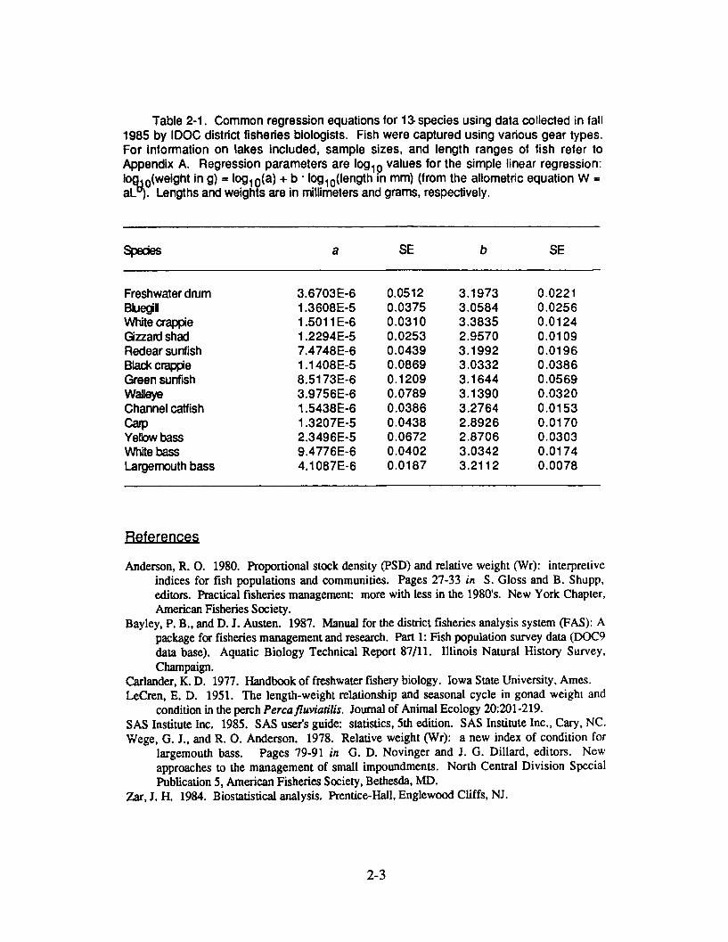
Table 2-1. Common regression equations for 13, species using data collected in fall1985 by IDOC district fisheries biologists. Fish were captured using various gear types.For Information on lakes included, sample sizes, and length ranges of fish refer toAppendix A. Regression parameters are loglo values for the simple linear regression:logjo(weight in g) = Iog10(a) + b - loglo(length in mm) (from the allometric equation W =aLu). Lengths and weights are in millimeters and grams, respectively.
Speces a SE b SE
Freshwater drum 3.6703E-6 0.0512 3.1973 0.0221Bluegill 1.3608E-5 0.0375 3.0584 0.0256White crappie 1.5011E-6 0.0310 3.3835 0.0124Gizzard shad 1.2294E-5 0.0253 2.9570 0.0109Redear sunfish 7.4748E-6 0.0439 3.1992 0.0196Black crappie 1.1408E-5 0.0869 3.0332 0.0386Green sunfish 8.5173E-6 0.1209 3.1644 0.0569Walleye 3.9756E-6 0.0789 3.1390 0.0320Channel catfish 1.5438E-6 0.0386 3.2764 0.0153Carp 1.3207E-5 0.0438 2.8926 0.0170Yellow bass 2.3496E-5 0.0672 2.8706 0.0303White bass 9.4776E-6 0.0402 3.0342 0.0174Largemouth bass 4.1087E-6 0.0187 3.2112 0.0078
Anderson, R. 0. 1980. Proportional stock density (PSD) and relative weight (Wr): interpretiveindices for fish populations and communities. Pages 27-33 in S. Gloss and B. Shupp,editors. Practical fisheries management: more with less in the 1980's. New York Chapter,American Fisheries Society.
Bayley, P. B., and D. J. Austen. 1987. Manual for the district fisheries analysis system (FAS): Apackage for fisheries management and research. Part 1: Fish population survey data (DOC9data base). Aquatic Biology Technical Report 87/11. Illinois Natural History Survey,Champaign.
Carlander, K. D. 1977. Handbook of freshwater fishery biology. Iowa State University, Ames.LeCren, E. D. 1951. The length-weight relationship and seasonal cycle in gonad weight and
condition in the perch Percafluviatilis. Journal of Animal Ecology 20:201-219.SAS Institute Inc. 1985. SAS user's guide: statistics, 5th edition. SAS Institute Inc., Cary, NC.Wege, G. J., and R. 0. Anderson. 1978. Relative weight (Wr): a new index of condition for
largemouth bass. Pages 79-91 in G. D. Novinger and J. G. Dillard, editors. Newapproaches to the management of small impoundments. North Central Division SpecialPublication 5, American Fisheries Society, Bethesda, MD.
Zar, J. H. 1984. Biostatistical analysis. Prentice-Hall, Englewood Cliffs, NJ.
2-3
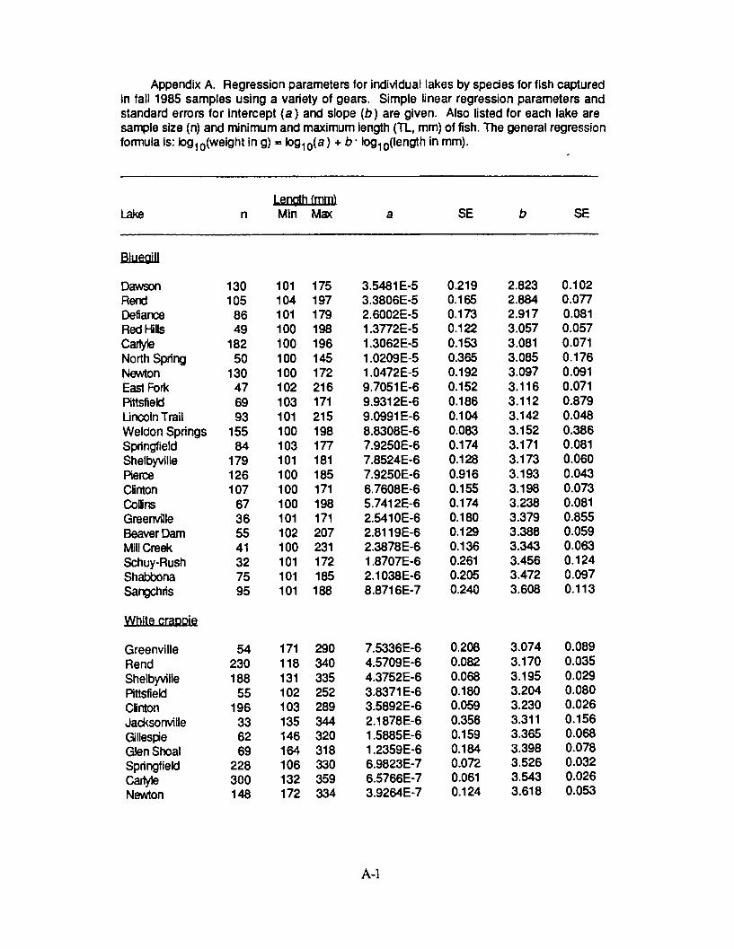
Appendix A. Regression parameters for individual lakes by species for fish capturedin fall 1985 samples using a variety of gears. Simple linear regression parameters andstandard errors for intercept (a) and slope (b) are given. Also listed for each lake aresample size (n) and minimum and maximum length (TL, mm) of fish. The general regressionformula is: log l o (weight in g) = log l o(a) + b - log 10(length in mm).
Length (mm)Lake n Min Max a SE b SE
Bluegill
DawsonRendDefianceRed HillsCartyleNorth SpringNewtonEast ForkPittsfieldUncoln TrailWeldon SpringsSpringfieldShelbyvillePierceClintonColinsGreenvilleBeaver DamMill CreekSchuy-RushShabbonaSangchris
White crappie
GreenvilleRendShelbyvillePittsfieldClintonJacksonvilleGillespeGlen ShoalSpringfieldCarlyeNewton
1301058649
18250
130476993
15584
17912610767365541327595
5423018855
196336269
228300148
101 175104 197101 179100 198100 196100 145100 172102 216103 171101 215100 198103 177101 181100 185100 171100 198101 171102 207100 231101 172101 185101 188
171 290118 340131 335102 252103 289135 344146 320164 318106 330132 359172 334
3.5481 E-53.3806E-52.6002E-51.3772E-51.3062E-51.0209E-51.0472E-59.7051 E-69.9312E-69.0991 E-68.8308E-67.9250E-67.8524E-67.9250E-66.7608E-65.7412E-62.541 OE-62.8119E-62.3878E-61.8707E-62.1038E-68.8716E-7
7.5336E-64.5709E-64.3752E-63.8371 E-63.5892E-62.1878E-61.5885E-61.2359E-66.9823E-76.5766E-73.9264E-7
0.2190.1650.1730.1220.1530.3650.1920.1520.1860.1040.0830.1740.1280.9160.1550.1740.1800.1290.1360.2610.2050.240
0.2080.0820.0680.1800.0590.3560.1590.1840.0720.0610.124
2.823 0.1022.884 0.0772.917 0.0813.057 0.0573.081 0.0713.085 0.1763.097 0.0913.116 0.0713.112 0.8793.142 0.0483.152 0.3863.171 0.0813.173 0.0603.193 0.0433.198 0.0733.238 0.0813.379 0.8553.388 0.0593.343 0.0633.456 0.1243.472 0.0973.608 0.113
3.074 0.0893.170 0.0353.195 0.0293.204 0.0803.230 0.0263.311 0.1563.365 0.0683.398 0.0783.526 0.0323.543 0.0263.618 0.053
A-1
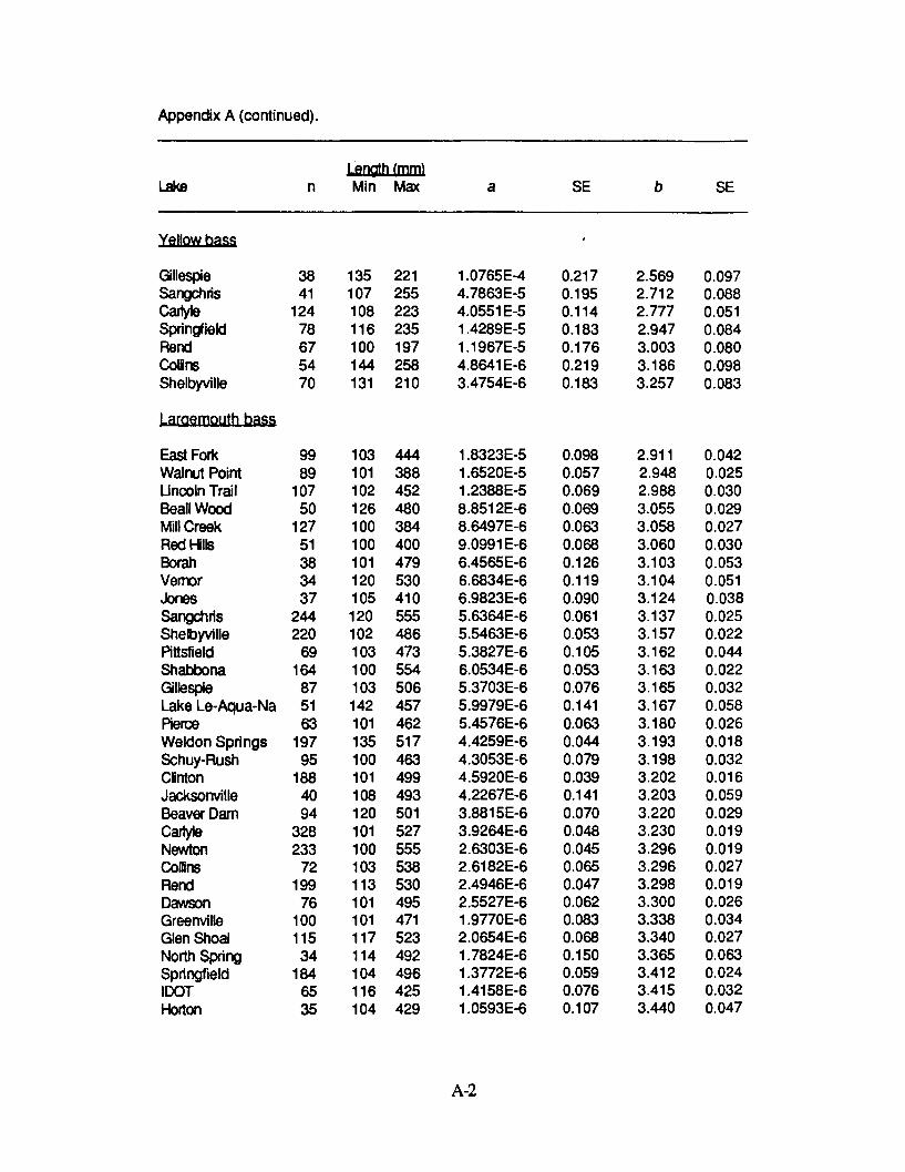
Appendix A (continued).
Lenath (mm)Lake n Min Max a SE b SE
38 135 22141 107 255
124 108 22378 116 23567 100 19754 144 25870 131 210
1.0765E-4 0.2174.7863E-5 0.1954.0551E-5 0.1141.4289E-5 0.1831.1967E-5 0.1764.8641 E-6 0.2193.4754E-6 0.183
2.569 0.0972.712 0.0882.777 0.0512.947 0.0843.003 0.0803.186 0.0983.257 0.083
Largemouth bass
East Fork 99 103 444Walnut Point 89 101 388Uncoln Trail 107 102 452Beall Wood 50 126 480Mill Creek 127 100 384Red Hills 51 100 400Borah 38 101 479Vemor 34 120 530Jones 37 105 410Sangchds 244 120 555Shelbyville 220 102 486Pittsfield 69 103 473Shabbona 164 100 554Gillespie 87 103 506Lake Le-Aqua-Na 51 142 457Pierce 63 101 462Weldon Springs 197 135 517Schuy-Rush 95 100 463Clinton 188 101 499Jacksonville 40 108 493Beaver Dam 94 120 501Cartyle 328 101 527Newton 233 100 555Collins 72 103 538Rend 199 113 530Dawson 76 101 495Greenville 100 101 471Glen Shoal 115 117 523North Spring 34 114 492Springfield 184 104 496IDOT 65 116 425Horton 35 104 429
1.8323E-5 0.0981.6520E-5 0.0571.2388E-5 0.0698.8512E-6 0.0698.6497E-6 0.0639.0991E-6 0.0686.4565E-6 0.1266.6834E-6 0.1196.9823E-6 0.0905.6364E-6 0.0615.5463E-6 0.0535.3827E-6 0.1056.0534E-6 0.0535.3703E-6 0.0765.9979E-6 0.1415.4576E-6 0.0634.4259E-6 0.0444.3053E-6 0.0794.5920E-6 0.0394.2267E-6 0.1413.8815E-6 0.0703.9264E-6 0.0482.6303E-6 0.0452.6182E-6 0.0652.4946E-6 0.0472.5527E-6 0.0621.9770E-6 0.0832.0654E-6 0.0681.7824E-6 0.1501.3772E-6 0.0591.4158E-6 0.0761.0593E-6 0.107
2.911 0.0422.948 0.0252.988 0.0303.055 0.0293.058 0.0273.060 0.0303.103 0.0533.104 0.0513.124 0.0383.137 0.0253.157 0.0223.162 0.0443.163 0.0223.165 0.0323.167 0.0583.180 0.0263.193 0.0183.198 0.0323.202 0.0163.203 0.0593.220 0.0293.230 0.0193.296 0.0193.296 0.0273.298 0.0193.300 0.0263.338 0.0343.340 0.0273.365 0.0633.412 0.0243.415 0.0323.440 0.047
A-2
GillespeSangchrisCa"yeSpringfieldRendColinsShelbyville
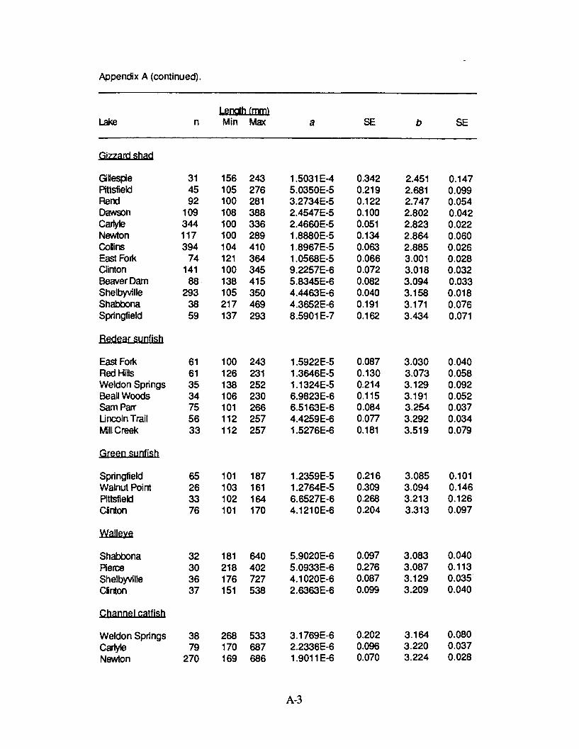
Appendix A (continued).
Length (mm)Lake n Min Max a SE b SE
GillespiePittsfieldRendDawsonCarlyleNewtonCollinsEast ForkClintonBeaver DamShelbyvilleShabbonaSpringfield
Redear sunfish
East ForkRed HillsWeldon SpringsBeall WoodsSam ParrLincoln TrailMill Creek
Green sunfish
SpringfieldWalnut PointPittsfieldCinton
ShabbonaPierceShelbyvilleCinton
Channel catfish
Weldon SpringsCartyleNewton
31 156 24345 105 27692 100 281
109 108 388344 100 336117 100 289394 104 410
74 121 364141 100 345
88 138 415293 105 350
38 217 46959 137 293
61 100 24361 126 23135 138 25234 106 23075 101 26656 112 25733 112 257
65 101 18726 103 16133 102 16476 101 170
32 181 64030 218 40236 176 72737 151 538
38 268 53379 170 687
270 169 686
1.5031 E-4 0.3425.0350E-5 0.2193.2734E-5 0.1222.4547E-5 0.1002.4660E-5 0.0511.8880E-5 0.1341.8967E-5 0.0631.0568E-5 0.0669.2257E-6 0.0725.8345E-6 0.0824.4463E-6 0.0404.3652E-6 0.1918.5901 E-7 0.162
1.5922E-5 0.0871.3646E-5 0.1301.1324E-5 0.2146.9823E-6 0.1156.5163E-6 0.0844.4259E-6 0.0771.5276E-6 0.181
1.2359E-5 0.2161.2764E-5 0.3096.6527E-6 0.2684.1210E-6 0.204
5.9020E-6 0.0975.0933E-6 0.2764.1020E-6 0.0872.6363E-6 0.099
3.1769E-6 0.2022.2336E-6 0.0961.9011E-6 0.070
2.451 0.1472.681 0.0992.747 0.0542.802 0.0422.823 0.0222.864 0.0602.885 0.0263.001 0.0283.018 0.0323.094 0.0333.158 0.0183.171 0.0763.434 0.071
3.030 0.0403.073 0.0583.129 0.0923.191 0.0523.254 0.0373.292 0.0343.519 0.079
3.085 0.1013.094 0.1463.213 0.1263.313 0.097
3.083 0.0403.087 0.1133.129 0.0353.209 0.040
3.164 0.0803.220 0.0373.224 0.028
A-3
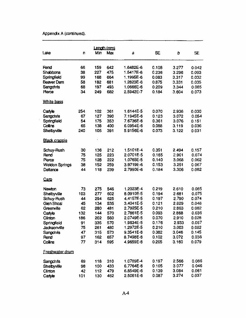
Appendix A (continued).
Length (mm)Lake n Min Max a SE b SE
RendShabbonaSpringfieldBeaver DamSangchrisPierce
White bass
CaryteSangchrisSpringfieldColinsShelbyville
Schuy-RushRendPierceWeldon SpringsDefiance
NewtonShelbyvilleSchuy-RushGlen ShoalGreenvilleCarlyleClintonSpringfieldJacksonvilleSangchrisRendCoins
Freshwater drum
66 159 64238 227 47599 168 66458 182 68168 197 49334 249 682
254 102 36167 127 39054 175 35365 138 400
240 105 391
30 136 21275 125 22375 128 22238 152 25944 118 239
73 275 546103 277 60244 294 62545 134 53562 280 481
132 144 570186 202 560
91 335 57075 261 48047 315 57397 162 65777 314 595
1.6482E-6 0.1081.5417E-6 0.2361.1995E-6 0.0831.2823E-6 0.8751.0666E-6 0.2092.5942E-7 0.184
1.6144E-5 0.0707.1945E-6 0.1237.6736E-6 0.3616.0954E-6 0.0885.9156E-6 0.073
1.5101E-4 0.3512.0701E-5 0.1651.0765E-5 0.1403.9719E-6 0.1532.7990E-6 0.184
1.2023E-4 0.2198.0910 E-5 0.1944.4157E-5 0.1973.4041E-5 0.1212.7925E-5 0.2102.7861 E-5 0.0932.0749E-5 0.0701.9634E-5 0.1761.2972E-5 0.2109.3541 E-6 0.3828.7498E-6 0.1024.9659E-6 0.205
3.277 0.0423.296 0.0933.317 0.0323.331 0.0353.344 0.0853.604 0.073
2.936 0.0303.072 0.0543.076 0.1513.119 0.0363.122 0.031
2.494 0.1572.901 0.0743.068 0.0623.251 0.0673.306 0.082
2.610 0.0852.681 0.0752.790 0.0742.829 0.0482.863 0.0822.868 0.0362.910 0.0282.933 0.0673.003 0.0823.046 0.1453.072 0.0383.160 0.079
69 118 31098 100 43342 112 479
101 130 482
1.0789E-4 0.1976.7764E-6 0.1056.8549E-6 0.1392.5061E-6 0.087
2.566 0.0863.077 0.0463.084 0.0613.274 0.037
A-4
SangchrisShelbyvilleCintonCartyle
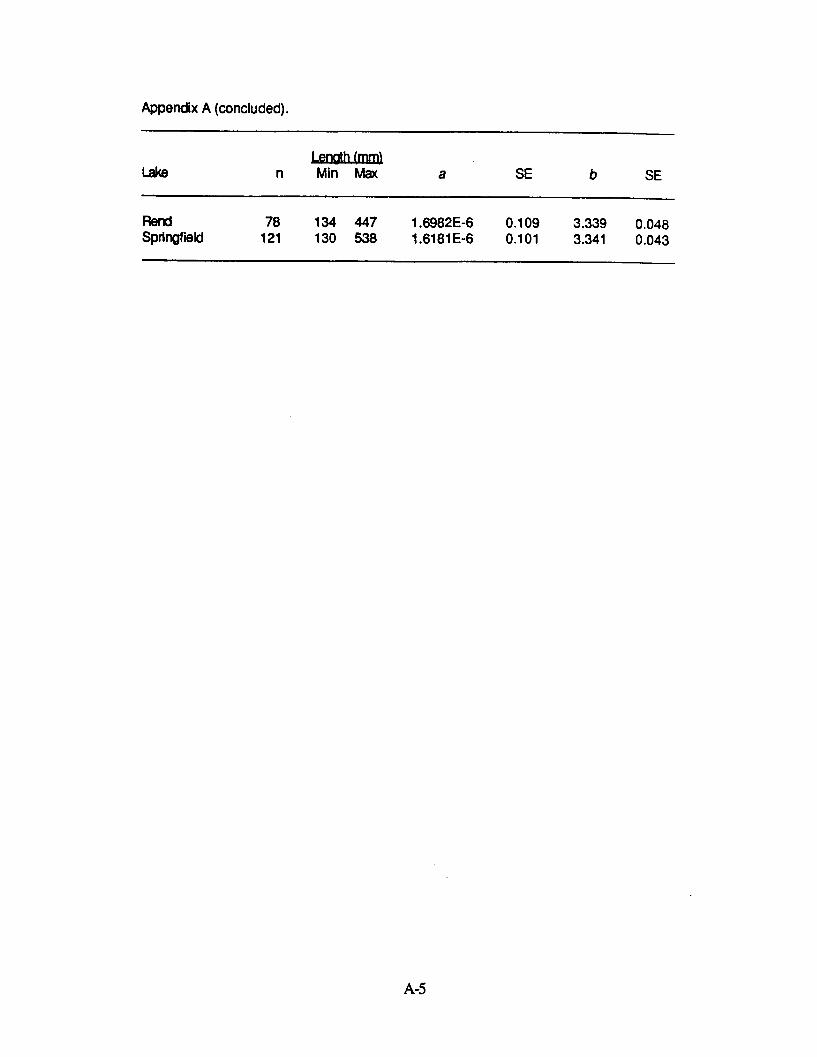
Appendix A (concluded).
Lerngh (mm)Lake n Min Max a SE b SE
Rend 78 134 447 1.6982E-6 0.109 3.339 0.048Springfield 121 130 538 1.6181E-6 0.101 3.341 0.043
A-5