Comparative Evaluation of Maximum Power Point Tracking Methods for Photovoltaic Systems

1

eietuectPw

taupm��ps

liibil

ifivt

J

Downloaded Fr

G. M. S. Azevedo

M. C. Cavalcantie-mail: [email protected]

K. C. Oliveira

F. A. S. Neves

Z. D. Lins

Departamento de Engenharia Elétrica e Sistemasde Potência,

Universidade Federal de Pernambuco,Rua Acadêmico Hélio Ramos, s/n,

Cidade Universitária,Recife, Pernambuco 50740-530, Brazil

Comparative Evaluation ofMaximum Power Point TrackingMethods for Photovoltaic SystemsThis paper presents a study of two maximum power point tracking methods for gridconnected photovoltaic systems. The best operation conditions for the perturbation andobservation and the incremental conductance methods are investigated in order to iden-tify the efficiency performances of these most popular maximum power point trackingmethods for photovoltaic systems. Improvements of these methods can be obtained withthe best adjustment of the sampling rate and the perturbation size, both in accordancewith the converter dynamics. Practical aspects about the incremental conductancemethod are discussed, and some modifications are proposed to overcome its problems. Aprocedure to determine the parameters is explained. This procedure helps to identifywhich method is better suited for grid connected photovoltaic systems with only oneconversion stage. The methods’ influences on the quality of the currents injected in thegrid are evaluated and compared. The performance improvement achieved with thechoice of the best parameters is proved by means of simulation and experimental resultsperformed on a low power test system. The simulation results have been obtained bymodeling a photovoltaic system in MATLAB. A simplified model was used that employs onlyparameters of interest and therefore decreases simulation time. Experimental results cor-responding to the operation of a grid connected photovoltaic converter controlled with adigital signal processor have been obtained. �DOI: 10.1115/1.3142827�

Keywords: energy conversion, photovoltaic power systems, solar energy, tracking

IntroductionPhotovoltaic �PV� energy is on the way to becoming a well-

stablished energy source in the coming decades. The PV energys particularly attractive as a renewable source for distributed gen-ration systems due to their relatively small size, noiseless opera-ion, ease of installation, and the possibility to put it close to theser. In this kind of application all available PV power is deliv-red to the electric grid and the system should operate in optimumonditions in order to improve its energy conversion. Thereforehe PV system needs a control system that senses variations in theV array condition and leads the system to a new operation pointhere the maximum power can be extracted.The voltage-power characteristic of a PV array is nonlinear and

ime-varying because of the variation caused by solar irradiancend temperature. Thus the linear control theory cannot be easilysed to obtain the voltage for operation on the maximum poweroint �MPP� of the PV array �1�. To solve this problem, severalethods have been developed to continuously track the MPP

2–17�. These methods are called maximum power point trackingMPPT�, becoming an essential part of a PV system. The mostopular MPPT methods in PV systems are perturbation and ob-ervation �P&O� and incremental conductance �Inc.Cond�.

In most applications two conversion stages are used for control-ing the PV array voltage. The first one is a dc/dc converter toncrease the PV voltage and, in some cases, to provide galvanicsolation. Moreover, this converter decouples the energy transferetween the PV array and the dc link capacitor. The second stages an inverter used to deliver the energy to the electric grid. The dcink voltage control and the grid currents inner control loops are

Contributed by the Solar Energy Engineering Division of ASME for publicationn the JOURNAL OF SOLAR ENERGY ENGINEERING. Manuscript received April 4, 2008;nal manuscript received September 26, 2008; published online June 10, 2009. Re-iew conducted by Antonio Marti Vega. Paper presented at the IEEE Power Elec-
ronics Specialists Conference 2008.
ournal of Solar Energy Engineering Copyright © 20

om: http://solarenergyengineering.asmedigitalcollection.asme.org/ on 05/0

being done by the inverter, while the MPPT control is performedby the dc/dc converter. However, in some applications it is pos-sible to use only one stage �one inverter� in order to increase thesystem efficiency. In that case, the control has three control loops:the outer MPPT control, followed by the dc link voltage controland the inner current control loop. Thus, the MPPT method andthe value of the dc link capacitor have great influence on thepower quality in the grid side. In most cases the MPPT methodperturbs the dc link voltage and if a large capacitor is used, muchmore energy must be exchanged with the grid, causing a pulsatingpower to be injected in the grid. On the other hand, if a smallcapacitor is used, variations in the available power of the PV arrayare transmitted to the grid.

MPPT techniques can be improved through the optimum ad-justment of the sampling rate and perturbation size �2�, both inaccordance with the converter dynamics. In this paper, a proce-dure to determine the optimum parameters of the P&O and In-c.Cond techniques is explained. This procedure helps to identifywhich technique is better suited for grid connected PV systemswith one stage. The techniques have been verified on a PV systemmodeled in MATLAB and the experimental results corresponding tothe operation of a grid connected PV converter controlled by adigital signal processor are also presented.

2 Photovoltaic System ModelTo evaluate the MPPT techniques, models of the PV array and

the inverter are necessary. The PV array model is based on thesingle-diode equivalent circuit. The inverter model is simplified totake into account only the dynamic behavior of the dc link voltagecontrol in order to achieve a reduced simulation time.

2.1 PV Array Model. The PV cell output characteristic canbe mathematically modeled by a double-exponential function,which is derived from the p-n junction physics. This function isgenerally accepted as a good model for the PV cells, especially
those made of polycrystalline silicon. The cells made of amor-
AUGUST 2009, Vol. 131 / 031006-109 by ASME

4/2014 Terms of Use: http://asme.org/terms

pcetedog

wrsfts

c

wS

0

Downloaded Fr

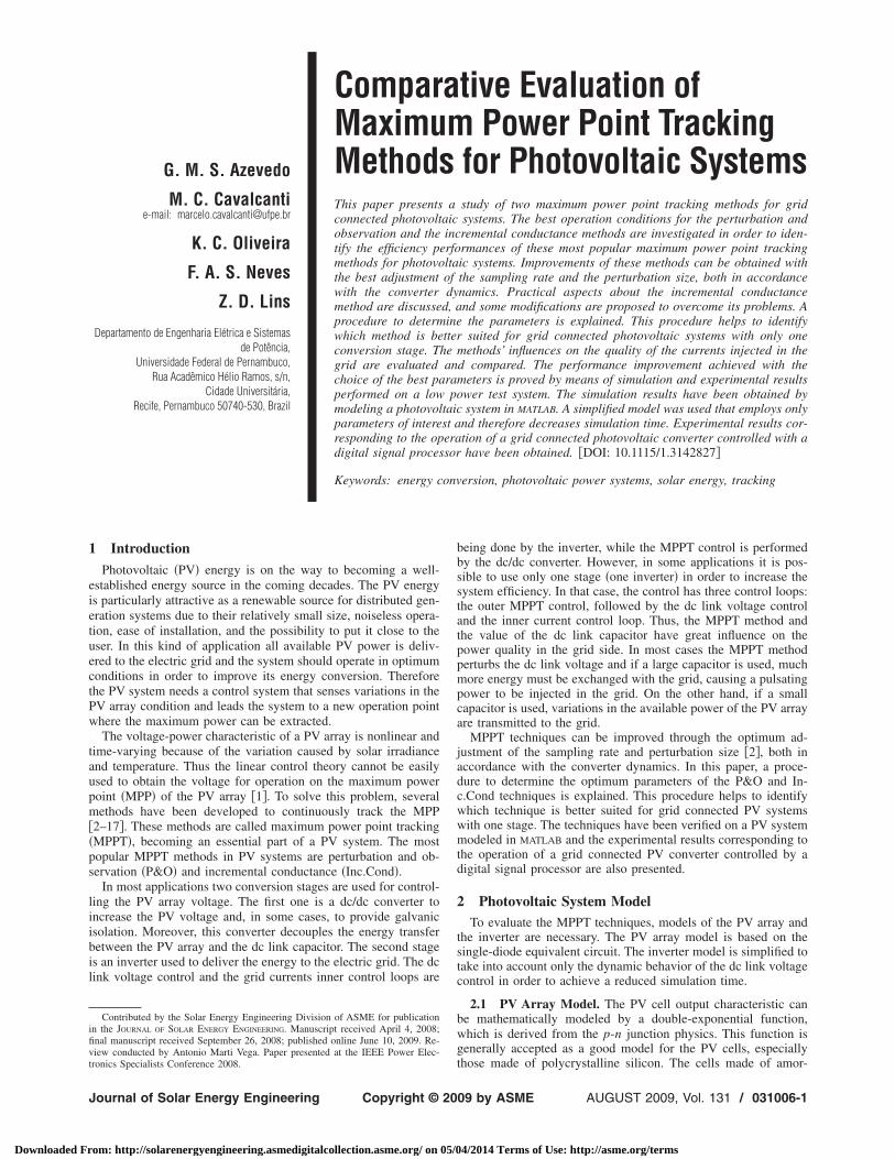
hous silicon do not exhibit a sharp “knee” in the characteristicurve as the crystalline types do, and therefore the single-xponential model provides a better fit to such cells �3�. Fromhese models, an equivalent circuit can be determined. Thequivalent circuit for the single-exponential model �or single-iode model� �4�, shown in Fig. 1 was used in this work. Theutput characteristic for constant temperature and irradiance isiven by the following equation �3–6�:

IPV = Ig − Io�exp� q

AkT�VPV + IPVRS�� − 1� −

VPV + IPVRS

RP�1�

here IPV and VPV are the PV cell output current and voltage,espectively; Ig is the photogenerated current; Io is the reverseaturation current; q is the charge of an electron; A is the idealityactor of the p-n junction; k is Boltzmann’s constant; T is theemperature in Kelvin; and RS and RP are the PV cell series andhunt resistances, respectively.

Considering the effects of irradiance and temperature on theurrent, the photogenerated current can be approximated as �3,4�

Ig = �1 + ki�T − TSTC��ISCSTC

S

SSTC�2�

here ki is the temperature coefficient of the short-circuit current,is the irradiance, and TSTC, ISCSTC

, and SSTC are the temperature,

Fig. 1 Equivalent circuit of the PV cell

Fig. 2 Grid conne

31006-2 / Vol. 131, AUGUST 2009


the short-circuit current, and irradiance in the standard test condi-tion �STC� provided by the manufacturer’s data sheet,respectively.

The saturation current does not depend on the irradiance con-ditions, but it shows strong dependence with the temperature,which can be approximated as �7�

Io = IoSTC� T

TSTC�3/A

exp�qEgo

Ak� 1

TSTC−

1

T�� 3�

where some simplifications, discussed in Ref. �6�, are considered.IoSTC

is the saturation current in the STC, and Ego is the band gapenergy of the semiconductor used in the cell.

The same model presented for the PV cell can be used for thePV array, although some modifications in the output current equa-tion are necessary. Considering np and ns as the number of paralleland series connections of the PV array, respectively, the followingmodification in Eq. �1� must be done.

IPV = npIg − npIo�exp� q

AkT

VPV + IPVRS

ns� − 1� −

VPV + IPVRS

RP

�4�The PV module manufacturer does not provide all parameters

of the model, but the unknown parameters can be extracted fromthe data sheet values through the procedure described in Ref. �4�.

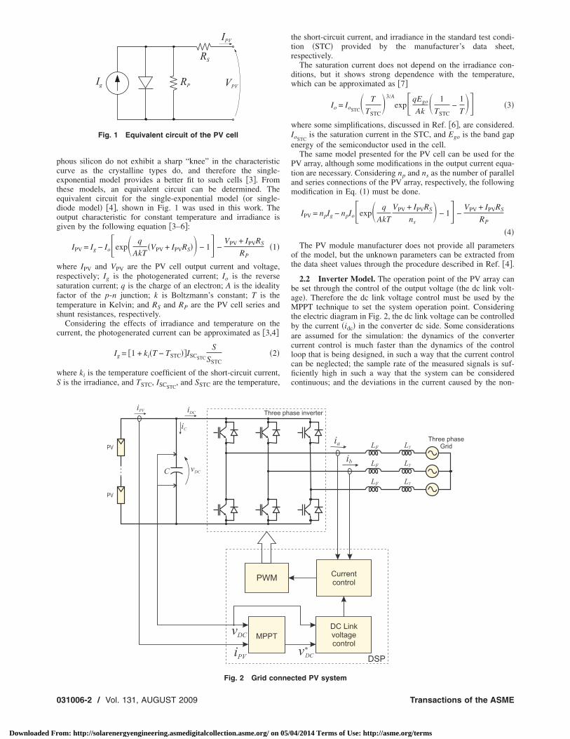
2.2 Inverter Model. The operation point of the PV array canbe set through the control of the output voltage �the dc link volt-age�. Therefore the dc link voltage control must be used by theMPPT technique to set the system operation point. Consideringthe electric diagram in Fig. 2, the dc link voltage can be controlledby the current �idc� in the converter dc side. Some considerationsare assumed for the simulation: the dynamics of the convertercurrent control is much faster than the dynamics of the controlloop that is being designed, in such a way that the current controlcan be neglected; the sample rate of the measured signals is suf-ficiently high in such a way that the system can be consideredcontinuous; and the deviations in the current caused by the non-

cted PV system

Transactions of the ASME


l

sacMf

w

msc

3

preiitloctdHoit

TtaTsdti�ua

J

Downloaded Fr

inearity of the ac loads do not disturb the dc link voltage.In Fig. 3, the block diagram of the dc link voltage control is

hown. kp is the proportional gain of the control loop. The PVrray current appears as a disturbance in the diagram, but it can beompensated in the control since it is measured to implement thePPT algorithm. From the block diagram, the following transfer

unction of the voltage control can be obtained:

T�s� =Vdc�s�Vdc

� �s�=

1

1 + s�vdc�5�

here �vdc=C /kp is the time constant of the voltage control.Using the PV array model, the MPPT algorithm and the inverterodel, as shown in Fig. 4, a simple and fast tool for evaluating the

ystem behavior is achieved. This tool has been used to define theriteria to choose the MPPT parameters.

Perturbation and ObservationIn the P&O technique, the power of the previous step is com-

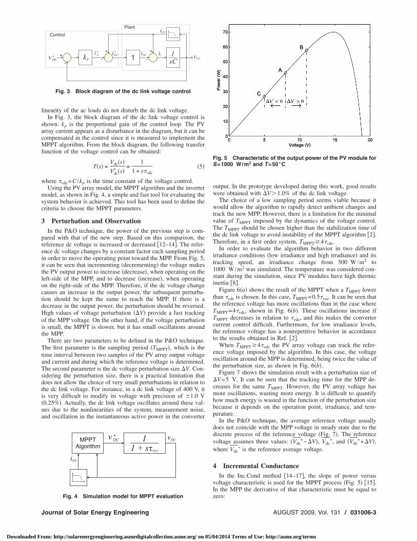
ared with that of the new step. Based on this comparison, theeference dc voltage is increased or decreased �12–14�. The refer-nce dc voltage changes by a constant factor each sampling periodn order to move the operating point toward the MPP. From Fig. 5,t can be seen that incrementing �decrementing� the voltage makeshe PV output power to increase �decrease�, when operating on theeft-side of the MPP, and to decrease �increase�, when operatingn the right-side of the MPP. Therefore, if the dc voltage changeauses an increase in the output power, the subsequent perturba-ion should be kept the same to reach the MPP. If there is aecrease in the output power, the perturbation should be reversed.igh values of voltage perturbation ��V� provide a fast trackingf the MPP voltage. On the other hand, if the voltage perturbations small, the MPPT is slower, but it has small oscillations aroundhe MPP.

There are two parameters to be defined in the P&O technique.he first parameter is the sampling period �TMPPT�, which is the

ime interval between two samples of the PV array output voltagend current and during which the reference voltage is determined.he second parameter is the dc voltage perturbation size �V. Con-idering the perturbation size, there is a practical limitation thatoes not allow the choice of very small perturbations in relation tohe dc link voltage. For instance, in a dc link voltage of 400 V, its very difficult to modify its voltage with precision of �1.0 V0.25%�. Actually, the dc link voltage oscillates around these val-es due to the nonlinearities of the system, measurement noise,nd oscillation in the instantaneous active power in the converter

Fig. 3 Block diagram of the dc link voltage control

Fig. 4 Simulation model for MPPT evaluation

ournal of Solar Energy Engineering


output. In the prototype developed during this work, good resultswere obtained with �V�1.0% of the dc link voltage.

The choice of a low sampling period seems viable because itwould allow the algorithm to rapidly detect ambient changes andtrack the new MPP. However, there is a limitation for the minimalvalue of TMPPT imposed by the dynamics of the voltage control.The TMPPT should be chosen higher than the stabilization time ofthe dc link voltage to avoid instability of the MPPT algorithm �2�.Therefore, in a first order system, TMPPT�4�vdc.

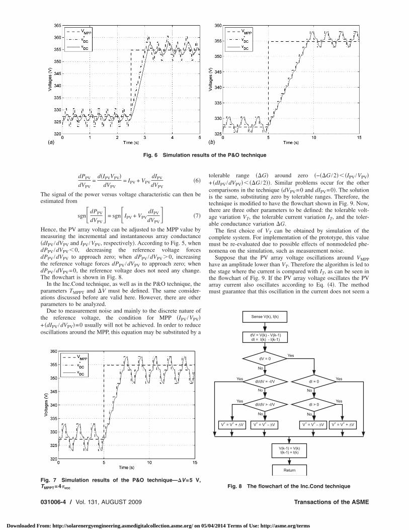
In order to evaluate the algorithm behavior in two differentirradiance conditions �low irradiance and high irradiance� and itstracking speed, an irradiance change from 500 W /m2 to1000 W /m2 was simulated. The temperature was considered con-stant during the simulation, since PV modules have high thermicinertia �8�.

Figure 6�a� shows the result of the MPPT when a TMPPT lowerthan �vdc is chosen. In this case, TMPPT=0.5�vcc. It can be seen thatthe reference voltage has more oscillations than in the case whereTMPPT=4�vdc, shown in Fig. 6�b�. These oscillations increase ifTMPPT decreases in relation to �vdc, and this makes the convertercurrent control difficult. Furthermore, for low irradiance levels,the reference voltage has a nonrepetitive behavior in accordanceto the results obtained in Ref. �2�.

When TMPPT�4�vdc the PV array voltage can track the refer-ence voltage imposed by the algorithm. In this case, the voltageoscillation around the MPP is determined, being twice the value ofthe perturbation size, as shown in Fig. 6�b�.

Figure 7 shows the simulation result with a perturbation size of�V=5 V. It can be seen that the tracking time for the MPP de-creases for the same TMPPT. However, the PV array voltage hasmore oscillations, wasting more energy. It is difficult to quantifyhow much energy is wasted in the function of the perturbation sizebecause it depends on the operation point, irradiance, and tem-perature.

In the P&O technique, the average reference voltage usuallydoes not coincide with the MPP voltage in steady state due to thediscrete process of the reference voltage �Fig. 7�. The referencevoltage assumes three values: �Vdc

�−�V�, Vdc�, and �Vdc

�+�V�,where Vdc

� is the reference average voltage.

4 Incremental ConductanceIn the Inc.Cond method �14–17�, the slope of power versus

voltage characteristic is used for the MPPT process �Fig. 5� �15�.In the MPP the derivative of that characteristic must be equal to

Fig. 5 Characteristic of the output power of the PV module forS=1000 W/m2 and T=50°C

zero:

AUGUST 2009, Vol. 131 / 031006-3


Te

Hm�ddtdT

pap

t+o

FT

0

Downloaded Fr

dPPV

dVPV=

d�IPVVPV�dVPV

= IPV + VPVdIPV

dVPV�6�

he signal of the power versus voltage characteristic can then bestimated from

sgn�dPPV

dVPV� = sgn�IPV + VPV

dIPV

dVPV� �7�

ence, the PV array voltage can be adjusted to the MPP value byeasuring the incremental and instantaneous array conductance

dIPV /dVPV and IPV /VPV, respectively�. According to Fig. 5, whenPPV /dVPV�0, decreasing the reference voltage forcesPPV /dVPV to approach zero; when dPPV /dVPV�0, increasing

he reference voltage forces dPPV /dVPV to approach zero; whenPPV /dVPV=0, the reference voltage does not need any change.he flowchart is shown in Fig. 8.In the Inc.Cond technique, as well as in the P&O technique, the

arameters TMPPT and �V must be defined. The same consider-tions discussed before are valid here. However, there are otherarameters to be analyzed.

Due to measurement noise and mainly to the discrete nature ofhe reference voltage, the condition for MPP �IPV /VPV��dIPV /dVPV�=0 usually will not be achieved. In order to reducescillations around the MPP, this equation may be substituted by a

Fig. 6 Simulation resu

ig. 7 Simulation results of the P&O technique—�V=5 V,
MPPT=4�vcc
31006-4 / Vol. 131, AUGUST 2009


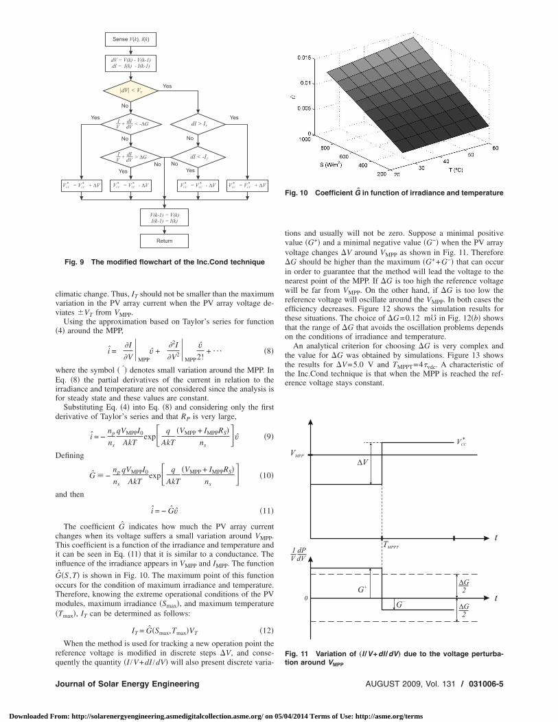
tolerable range ��G� around zero �−��G /2�� IPV /VPV�+ �dIPV /dVPV�� G /2��. Similar problems occur for the othercomparisons in the technique �dVPV=0 and dIPV=0�. The solutionis the same, substituting zero by tolerable ranges. Therefore, thetechnique is modified to have the flowchart shown in Fig. 9. Now,there are three other parameters to be defined: the tolerable volt-age variation VT, the tolerable current variation IT, and the toler-able conductance variation �G.

The first choice of VT can be obtained by simulation of thecomplete system. For implementation of the prototype, this valuemust be re-evaluated due to possible effects of nonmodeled phe-nomena on the simulation, such as measurement noise.

Suppose that the PV array voltage oscillations around VMPPhave an amplitude lower than VT. Therefore the algorithm is led tothe stage where the current is compared with IT, as can be seen inthe flowchart of Fig. 9. If the PV array voltage oscillates the PVarray current also oscillates according to Eq. �4�. The methodmust guarantee that this oscillation in the current does not seem a

of the P&O technique
lts
Fig. 8 The flowchart of the Inc.Cond technique



cvv

�

wEif

d

D

a

cTii

GoTm�

rq

J

Downloaded Fr

limatic change. Thus, IT should not be smaller than the maximumariation in the PV array current when the PV array voltage de-iates �VT from VMPP.

Using the approximation based on Taylor’s series for function4� around the MPP,

i = �I

�V

MPPv + �2I

�V2MPP

v2!

+ ¯ �8�

here the symbol � ˆ� denotes small variation around the MPP. Inq. �8� the partial derivatives of the current in relation to the

rradiance and temperature are not considered since the analysis isor steady state and these values are constant.

Substituting Eq. �4� into Eq. �8� and considering only the firsterivative of Taylor’s series and that RP is very large,

i = −np

ns

qVMPPI0

AkTexp� q

AkT

�VMPP + IMPPRS�ns

�v �9�

efining

G −np

ns

qVMPPI0

AkTexp� q

AkT

�VMPP + IMPPRS�ns

� �10�

nd then

i = − Gv �11�

The coefficient G indicates how much the PV array currenthanges when its voltage suffers a small variation around VMPP.his coefficient is a function of the irradiance and temperature and

t can be seen in Eq. �11� that it is similar to a conductance. Thenfluence of the irradiance appears in VMPP and IMPP. The functionˆ �S ,T� is shown in Fig. 10. The maximum point of this functionccurs for the condition of maximum irradiance and temperature.herefore, knowing the extreme operational conditions of the PVodules, maximum irradiance �Smax�, and maximum temperature

Tmax�, IT can be determined as follows:

IT = G�Smax,Tmax�VT �12�When the method is used for tracking a new operation point the

eference voltage is modified in discrete steps �V, and conse-

Fig. 9 The modified flowchart of the Inc.Cond technique

uently the quantity �I /V+dI /dV� will also present discrete varia-

ournal of Solar Energy Engineering


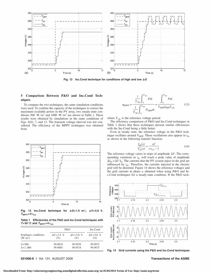
tions and usually will not be zero. Suppose a minimal positivevalue �G+� and a minimal negative value �G−� when the PV arrayvoltage changes �V around VMPP as shown in Fig. 11. Therefore�G should be higher than the maximum �G++G−� that can occurin order to guarantee that the method will lead the voltage to thenearest point of the MPP. If �G is too high the reference voltagewill be far from VMPP. On the other hand, if �G is too low thereference voltage will oscillate around the VMPP. In both cases theefficiency decreases. Figure 12 shows the simulation results forthese situations. The choice of �G=0.12 m� in Fig. 12�b� showsthat the range of �G that avoids the oscillation problems dependson the conditions of irradiance and temperature.

An analytical criterion for choosing �G is very complex andthe value for �G was obtained by simulations. Figure 13 showsthe results for �V=5.0 V and TMPPT=4�vdc. A characteristic ofthe Inc.Cond technique is that when the MPP is reached the ref-erence voltage stays constant.

Fig. 10 Coefficient G in function of irradiance and temperature

Fig. 11 Variation of „I /V+dI /dV… due to the voltage perturba-
tion around VMPP
AUGUST 2009, Vol. 131 / 031006-5


5n

wmdrFsf

r c

FT

TT

I�

SS

0

Downloaded Fr

Comparison Between P&O and Inc.Cond Tech-iquesTo compare the two techniques, the same simulation conditions

ere used. To confirm the capacity of the techniques to extract theaximum available power in the PV array, two steady-state con-

itions 500 W /m2 and 1000 W /m2 are shown in Table 1. Theseesults were obtained by simulations in the same conditions ofigs. 6�b�, 7, and 13. The transient voltage interval was not con-idered. The efficiency of the MPPT techniques was obtainedrom

Fig. 12 Inc.Cond technique fo

ig. 13 Inc.Cond technique for �G=1.5 m�, �V=5.0 V,MPPT=4�vcc

able 1 Efficiencies of the P&O and Inc.Cond techniques with=50°C and TMPPT=4�vcc

rradiance conditionsW /m2�

P&O Inc.Cond

�V=2.5 V�%�

�V=5.0 V�%�

�V=5.0 V�%�

=500 99.9870 99.9559 99.9975=1,000 99.9885 99.9518 99.9875

31006-6 / Vol. 131, AUGUST 2009


�MPPT =

1

Tvdc�

0

Tvdc

Pdt

1

Tvdc�

0

Tvdc

PMPPdt

=

�0

Tvdc

Pdt

VMPPIMPPTvdc�13�

where Tvdc is the reference voltage period.The efficiency comparison of P&O and Inc.Cond techniques in

Table 1 shows that these techniques present similar efficiencieswith the Inc.Cond being a little better.

Even in steady state, the reference voltage in the P&O tech-nique oscillates around VMPP. These oscillations also appear in idcas shown in the following transfer function:

Idc�s�Vdc

� �s�=

sC

s�vcc − 1�14�

The reference voltage varies in steps of amplitude �V. The corre-sponding variations in idc will reach a peak value of amplitude�Idc=�V kp. The currents that the PV system inject in the grid areinfluenced by idc. Therefore, the currents injected in the electricgrid will be distorted. Figure 14 shows the reference voltages andthe grid currents in phase a obtained when using P&O and In-c.Cond techniques for a steady-state condition. If the P&O tech-

onditions of high and low �G

Fig. 14 Grid currents using the P&O and Inc.Cond techniques



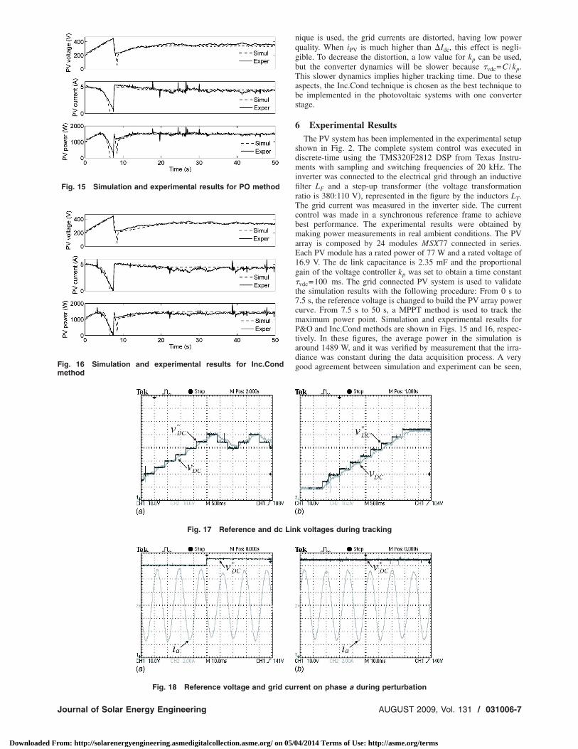
Fig. 15 Simulation and experimental results for PO method

Fm

Fig. 18 Reference voltage and grid cur

Journal of Solar Energy Engineering

Downloaded From: http://solarenergyengineering.asmedigitalcollection.asme.org/ on 05/0

nique is used, the grid currents are distorted, having low powerquality. When iPV is much higher than �Idc, this effect is negli-gible. To decrease the distortion, a low value for kp can be used,but the converter dynamics will be slower because �vdc=C /kp.This slower dynamics implies higher tracking time. Due to theseaspects, the Inc.Cond technique is chosen as the best technique tobe implemented in the photovoltaic systems with one converterstage.

6 Experimental ResultsThe PV system has been implemented in the experimental setup

shown in Fig. 2. The complete system control was executed indiscrete-time using the TMS320F2812 DSP from Texas Instru-ments with sampling and switching frequencies of 20 kHz. Theinverter was connected to the electrical grid through an inductivefilter LF and a step-up transformer �the voltage transformationratio is 380:110 V�, represented in the figure by the inductors LT.The grid current was measured in the inverter side. The currentcontrol was made in a synchronous reference frame to achievebest performance. The experimental results were obtained bymaking power measurements in real ambient conditions. The PVarray is composed by 24 modules MSX77 connected in series.Each PV module has a rated power of 77 W and a rated voltage of16.9 V. The dc link capacitance is 2.35 mF and the proportionalgain of the voltage controller kp was set to obtain a time constant�vdc=100 ms. The grid connected PV system is used to validatethe simulation results with the following procedure: From 0 s to7.5 s, the reference voltage is changed to build the PV array powercurve. From 7.5 s to 50 s, a MPPT method is used to track themaximum power point. Simulation and experimental results forP&O and Inc.Cond methods are shown in Figs. 15 and 16, respec-tively. In these figures, the average power in the simulation isaround 1489 W, and it was verified by measurement that the irra-diance was constant during the data acquisition process. A verygood agreement between simulation and experiment can be seen,

k voltages during tracking

ig. 16 Simulation and experimental results for Inc.Condethod

Fig. 17 Reference and dc Lin

rent on phase a during perturbation

AUGUST 2009, Vol. 131 / 031006-7


stvtMva

cT1sFot

7

tdprtpthTblwducnmgn

R

0

Downloaded Fr

howing that the PV array model used for comparing the MPPTechniques is valid. Figures 17�a� and 17�b� show the referenceoltage and the dc link voltage during the tracking of the MPP forhe P&O and Inc.Cond methods, respectively. In both results, the

PPT parameters are TMPPT=4�vdc=400 ms and �V=5 V. Aery good agreement can also be seen between simulation �Figs. 7nd 13� and experimental results.

Figure 18�a� shows the instant when the voltage reference ishanged by the P&O method, when it operates in steady state.his change causes a small dip in the grid current as shown in Fig.8�a�. When Inc.Cond is used, the reference voltage becomes con-tant resulting in a constant grid current amplitude as shown inig. 18�b�. These figures were obtained under identical conditionsf irradiance and temperature. Again, a very good agreement be-ween simulation �Fig. 14� and experiment can be seen.

ConclusionThis paper has discussed two maximum power point tracking

echniques. Principles of operation and main features have beeniscussed for a better understanding of each possibility. In thisaper, the model of the photovoltaic array is simple and its pa-ameters can be determined by the data supplied by the manufac-urer, allowing easy definition of the parameters of maximumower point tracking techniques. The implementation of the per-urbation and observation algorithm in software is very simple,aving only one multiplication and few sums and comparisons.he incremental conductance algorithm is a little more complex,ut both algorithms can be implemented in low cost microcontrol-ers. The grid connected photovoltaic system presented in thisork demands high computational capacity of the control systemue to the current compensations and a digital signal processor issed. Using digital signal processors the differences about theomputational effort of the maximum power point tracking tech-iques can be neglected. Therefore, the better results of the incre-ental conductance method related to the current injected in the

rid indicate that this method is more suitable for the grid con-ected photovoltaic systems.

eferences�1� Hua, C., Lin, J., and Shen, C., 2002, “Robust Control for Maximum Power

Point Tracking in Photovoltaic Power System,” Power Conversion Conference,

31006-8 / Vol. 131, AUGUST 2009


pp. 827–832.�2� Femia, N., Petrone, G., Spagnuolo, G., and Vitelli, M., 2005, “Optimization of

Perturb and Observe Maximum Power Point Tracking Method,” IEEE Trans.Power Electron., 20�4�, pp. 963–973.

�3� Gow, J. A., and Manning, C. D., 1999, “Development of a Photovoltaic ArrayModel for Use in Power-Electronics Simulation Studies,” IEE Proc.: Electr.Power Appl., 146�2�, pp. 193–200.

�4� Xiao, W., Dunford, W. G., and Capel, A., 2004, “A Novel Modeling Methodfor Photovoltaic Cells,” IEEE Power Electronics Specialists Conference, Vol.3, pp. 1950–1956.

�5� Esram, T., and Chapman, P. L., 2007, “Comparison of Photovoltaic ArrayMaximum Power Point Tracking Techniques,” IEEE Trans. Energy Convers.,22�2�, pp. 439–449.

�6� Matagne, E., Chenni, R., and El Bachtiri, R., 2007, “A Photovoltaic CellModel Based on Nominal Data Only,” International Conference on PowerEngineering, Energy and Electrical Drives, Apr., pp. 562–565.

�7� Yu, G. J., Jung, Y. S., Choi, J. Y., Choi, I., Song, J. H., and Kim, G. S., 2002,“A Novel Two-Mode MPPT Control Algorithm Based on Comparative Studyof Existing Algorithms,” IEEE Photovoltaic Specialists Conference, pp. 1531–1534.

�8� Liu, S., and Dougal, R. A., 2002, “Dynamic Multiphysics Model for SolarArray,” IEEE Trans. Energy Convers., 17�2�, pp. 285–294.

�9� Kislovski, A. S., 1993, “Power Tracking Methods in Photovoltaic Applica-tions,” IEEE Power Conversion Proceedings, pp. 513–528.

�10� Radziemska, E., and Klugmann, E., 2006, “Photovoltaic Maximum PowerPoint Varying With Illumination and Temperature,” ASME J. Sol. EnergyEng., 128, pp. 34–39.

�11� El-Aal, A. M., Schmid, J., Bard, J., and Caselitz, P., 2006, “Modeling andOptimizing the Size of the Power Conditioning Unit for Photovoltaic Sys-tems,” ASME J. Sol. Energy Eng., 128, pp. 40–44.

�12� Liu, X., and Lopes, L., 2004, “An Improved Perturbation and ObservationMaximum Power Point Tracking Algorithm for PV Arrays,” IEEE Power Elec-tronics Specialists Conference, pp. 2005–2010.

�13� Hua, C., Lin, J., and Shen, C., 1998, “Implementation of a DSP-ControlledPhotovoltaic System With Peak Power Tracking,” IEEE Trans. Ind. Electron.,45�1�, pp. 99–107.

�14� Hohm, D., and Ropp, M., 2000, “Comparative Study of Maximum PowerPoint Tracking Algorithms Using an Experimental, Programmable, MaximumPower Point Tracking Test Bed,” IEEE Photovoltaic Specialists Conference,pp. 1699–1702.

�15� Hussein, K., Muta, I., Hoshino, T., and Osakada, M., 1995, “Maximum Pho-tovoltaic Power Tracking: An Algorithm for Rapidly Changing AtmosphericConditions,” IEE Proc.: Gener. Transm. Distrib., 142, pp. 59–64.

�16� Kuo, Y., Liang, T., and Chen, J., 2001, “Novel Maximum Power-Point-Tracking Controller for Photovoltaic Energy Conversion System,” IEEE Trans.Ind. Electron., 48�3�, pp. 594–601.

�17� Kim, T., Ahn, H., Park, S., and Lee, Y., 2001, “A Novel Maximum PowerPoint Tracking Control for Photovoltaic Power System Under Rapidly Chang-ing Solar Radiation,” IEEE International Symposium on Industrial Electronics,
pp. 1011–1014.


Documents

Comparative Evaluation of Maximum Power Point Tracking Methods for Photovoltaic Systems