Comparing Corpora

Comparing Corpora

ADAM KILGARRIFFITRI, University of Brighton

Corpus linguistics lacks strategies for describing and comparing corpora. Cur-rently most descriptions of corpora are textual, and questions such as ‘what sortof a corpus is this?’, or ‘how does this corpus compare to that?’ can only be an-swered impressionistically. This paper considers various ways in which differentcorpora can be compared more objectively. First we address the issue, ‘whichwords are particularly characteristic of a corpus?’, reviewing and critiquing thestatistical methods which have been applied to the question and proposing theuse of the Mann-Whitney ranks test. Results of two corpus comparisons usingthe ranks test are presented. Then, we consider measures for corpus similarity.After discussing limitations of the idea of corpus similarity, we present a methodfor evaluating corpus similarity measures. We consider several measures and es-tablish that a χ2-based one performs best. All methods considered in this paperare based on word and ngram frequencies; the strategy is defended.

KEYWORDS: similarity, homogeneity, word frequency

1. Introduction

There is a void at the heart of corpus linguistics. The name puts ‘corpus’ atthe centre of the discipline.1 In any science, one expects to find a useful ac-count of how its central constructs are taxonomised and measured, and howthe subspecies compare. But to date, corpus linguistics has measured corporaonly in the most rudimentary ways, ways which provide no leverage on thedifferent kinds of corpora there are. The terms it has used for taxonomisingcorpora have been unrelated to any measurement: a corpus is described as

INTERNATIONAL JOURNAL OF CORPUS LINGUISTICS Vol. 6(1), 2001. 97–133 John Benjamins Publishing Co.

98 ADAM KILGARRIFF

“Wall Street Journal” or “transcripts of business meetings” or “foreign learn-ers’ essays (intermediate grade)”, but if a new corpus is to be compared withexisting ones, there are no methods for quantifying how it stands in relationto them.

The lack arises periodically wherever corpora are discussed. If an inter-esting finding is generated using one corpus, for what other corpora does ithold? On the CORPORA mailing list (http://www.hd.vib.no/corpora), the issueis aired every few months. Recently it arose in relation to the size of corpusthat had to be gathered to test certain hypotheses: a reference was made toBiber (1990 and 1993a) where corpus sizes for various tasks are discussed.The next question is, what sort of corpus did Biber’s figures relate to? If thecorpus is highly homogeneous, less data will be required. But there are noestablished measures for homogeneity.

Two salient questions are “how similar are two corpora”, and “in whatways do two corpora differ?” The second question has a longer history to it,so is taken first. Researchers have wanted to answer it for a variety of reasons,in a variety of academic disciplines. In the first part of the paper, the statisticaland other techniques used in linguistics, social science, information retrieval,natural language processing and speech processing are critically reviewed.

Almost all the techniques considered work with word frequencies. Whilea full comparison between any two corpora would of course cover many othermatters, the concern of this paper is with the statistical framework. Reliablestatistics depend on features that are reliably countable and, foremost amongstthese, in language corpora, are words.

The first part of the paper surveys and critiques the statistical methodswhich have been applied to finding the words which are most characteristicof one corpus as against another, and identifies the Mann-Whitney ranks testas a suitable technique. The next part goes on to use it to compare Britishand American English, and male and female conversational speech.

We then move on to address corpus similarity directly. Measures areneeded not only for theoretical and research work, but also to address practi-cal questions that arise wherever corpora are used: is a new corpus sufficientlydifferent from available ones, to make it worth acquiring? When will a gram-mar based on one corpus be valid for another? How much will it cost to porta Natural Language Processing (NLP) application from one domain, withone corpus, to another, with another? Various measures for corpus similarity

COMPARING CORPORA 99

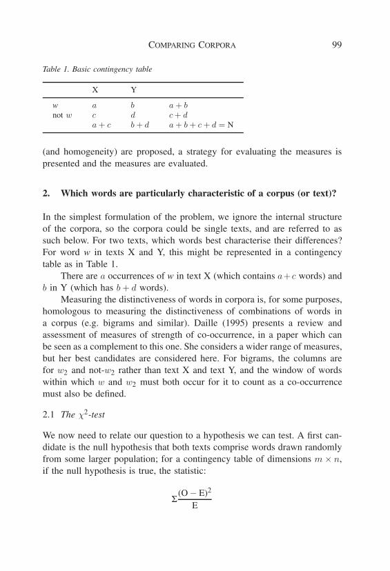
Table 1. Basic contingency table

X Y

w a b a + bnot w c d c + d

a + c b + d a + b + c + d = N

(and homogeneity) are proposed, a strategy for evaluating the measures ispresented and the measures are evaluated.

2. Which words are particularly characteristic of a corpus (or text)?

In the simplest formulation of the problem, we ignore the internal structureof the corpora, so the corpora could be single texts, and are referred to assuch below. For two texts, which words best characterise their differences?For word w in texts X and Y, this might be represented in a contingencytable as in Table 1.

There are a occurrences of w in text X (which contains a+c words) andb in Y (which has b + d words).

Measuring the distinctiveness of words in corpora is, for some purposes,homologous to measuring the distinctiveness of combinations of words ina corpus (e.g. bigrams and similar). Daille (1995) presents a review andassessment of measures of strength of co-occurrence, in a paper which canbe seen as a complement to this one. She considers a wider range of measures,but her best candidates are considered here. For bigrams, the columns arefor w2 and not-w2 rather than text X and text Y, and the window of wordswithin which w and w2 must both occur for it to count as a co-occurrencemust also be defined.

2.1 The χ2-test

We now need to relate our question to a hypothesis we can test. A first can-didate is the null hypothesis that both texts comprise words drawn randomlyfrom some larger population; for a contingency table of dimensions m × n,if the null hypothesis is true, the statistic:

Σ(O − E)2

E

100 ADAM KILGARRIFF

(where O is the observed value, E is the expected value calculated on thebasis of the joint corpus, and the sum is over the cells of the contingencytable) will be χ2-distributed with (m− 1)× (n− 1) degrees of freedom.2 Forour 2×2 contingency table the statistic has one degree of freedom and Yate’scorrection is applied, subtracting 1

2 from |O−E| before squaring. Whereverthe statistic is greater than the critical value of 7.88, we conclude with 99.5%confidence that, in terms of the word we are looking at, X and Y are notrandom samples of the same larger population.

This is the strategy adopted by Hofland and Johansson (1982), Leechand Fallon (1992), to identify where words are more common in British thanAmerican English or vice versa. X was the Lancaster-Oslo-Bergen (LOB)corpus, Y was the Brown, and, in the table where the comparison is made,words are marked a where the null hypothesis was defeated with 99.9%confidence, b where it was defeated with 99% confidence, and c where it wasdefeated with 95% confidence. Rayson, Leech, and Hodges (1997) use theχ2 similarly for the analysis of the conversation component of the BritishNational Corpus (BNC).3

Looking at the LOB-Brown comparison, we find that this is true for verymany words, and for almost all very common words. Much of the time, thenull hypothesis is defeated. At a first pass, this would appear to demonstratethat all those words have systematically different patterns of usage in Britishand American English, the two types that the two corpora were designedto represent. A first experiment was designed to check whether this was anappropriate interpretation.

2.2 Experiment: same-genre subsets of the BNC

If the χ2-test was picking up on interesting differences between the corpora,then, if there were no such differences, the null hypothesis would not bedefeated. To test this, I took two corpora which were indisputably of the samelanguage type: each was a random subset of the written part of the BritishNational Corpus (BNC). The sampling was as follows: all texts shorter than20,000 words were excluded. This left 820 texts. Half the texts were thenrandomly assigned to each of two subcorpora.

If we randomly assign words (as opposed to documents) to the onecorpus or the other, then we have a straightforward random distribution, with


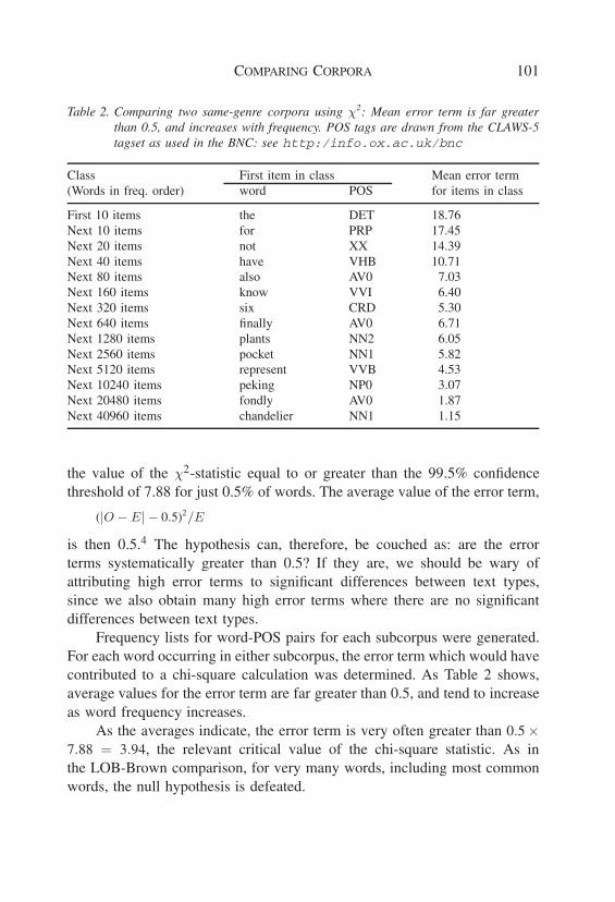
Table 2. Comparing two same-genre corpora using χ2: Mean error term is far greaterthan 0.5, and increases with frequency. POS tags are drawn from the CLAWS-5tagset as used in the BNC: see http:/info.ox.ac.uk/bnc

Class First item in class Mean error term(Words in freq. order) word POS for items in class

First 10 items the DET 18.76Next 10 items for PRP 17.45Next 20 items not XX 14.39Next 40 items have VHB 10.71Next 80 items also AV0 7.03Next 160 items know VVI 6.40Next 320 items six CRD 5.30Next 640 items finally AV0 6.71Next 1280 items plants NN2 6.05Next 2560 items pocket NN1 5.82Next 5120 items represent VVB 4.53Next 10240 items peking NP0 3.07Next 20480 items fondly AV0 1.87Next 40960 items chandelier NN1 1.15

the value of the χ2-statistic equal to or greater than the 99.5% confidencethreshold of 7.88 for just 0.5% of words. The average value of the error term,

(|O − E| − 0.5)2/E

is then 0.5.4 The hypothesis can, therefore, be couched as: are the errorterms systematically greater than 0.5? If they are, we should be wary ofattributing high error terms to significant differences between text types,since we also obtain many high error terms where there are no significantdifferences between text types.

Frequency lists for word-POS pairs for each subcorpus were generated.For each word occurring in either subcorpus, the error term which would havecontributed to a chi-square calculation was determined. As Table 2 shows,average values for the error term are far greater than 0.5, and tend to increaseas word frequency increases.

As the averages indicate, the error term is very often greater than 0.5 ×7.88 = 3.94, the relevant critical value of the chi-square statistic. As inthe LOB-Brown comparison, for very many words, including most commonwords, the null hypothesis is defeated.

102 ADAM KILGARRIFF

2.2.1 DiscussionThis reveals a bald, obvious fact about language. Words are not selected atrandom. There is no a priori reason to expect them to behave as if they hadbeen, and indeed they do not. The LOB-Brown differences cannot in generalbe interpreted as British-American differences: it is in the nature of languagethat any two collections of texts, covering a wide range of registers (andcomprising, say, less than a thousand samples of over a thousand words each)will show such differences. While it might seem plausible that oddities wouldin some way balance out to give a population that was indistinguishable fromone where the individual words (as opposed to the texts) had been randomlyselected, this turns out not to be the case.

Let us look closer at why this occurs. A key word in the last paragraphis ‘indistinguishable’. In hypothesis testing, the objective is generally to seeif the population can be distinguished from one that has been randomlygenerated—or, in our case, to see if the two populations are distinguishablefrom two populations which have been randomly generated on the basis ofthe frequencies in the joint corpus. Since words in a text are not random, weknow that our corpora are not randomly generated. The only question, then,is whether there is enough evidence to say that they are not, with confidence.In general, where a word is more common, there is more evidence. This iswhy a higher proportion of common words than of rare ones defeat the nullhypothesis. As one statistics textbook puts it:

None of the null hypotheses we have considered with respect to goodness offit can be exactly true, so if we increase the sample size (and hence the valueof χ2) we would ultimately reach the point when all null hypotheses wouldbe rejected. All that the χ2 test can tell us, then, is that the sample size is toosmall to reject the null hypothesis! (Owen and Jones 1977: 359)

For large corpora and common words, the sample size is no longer too small.The χ2-test can be used for all sizes of contingency tables, so can be used

to compare two corpora in respect of a set of words, large or small, ratherthan one-word-at-a-time. In all the experiments in which I have comparedcorpora in respect of a substantial set of words, the null hypothesis has beendefeated (by a huge margin).

The original question was not about which words are random but aboutwhich words are most distinctive. It might seem that these are converses, andthat the words with the highest values for the error term—those for whichthe null hypothesis is most soundly defeated—will also be the ones which


are most distinctive to one corpus or the other. Where the overall frequencyfor a word in the joint corpus is held constant, this is valid, but as we haveseen, for very common words, high χ2 values are associated with the sheerquantity of evidence and are not necessarily associated with a pre-theoreticalnotion of distinctiveness (and for words with expected frequency less than5, the test is not usable).

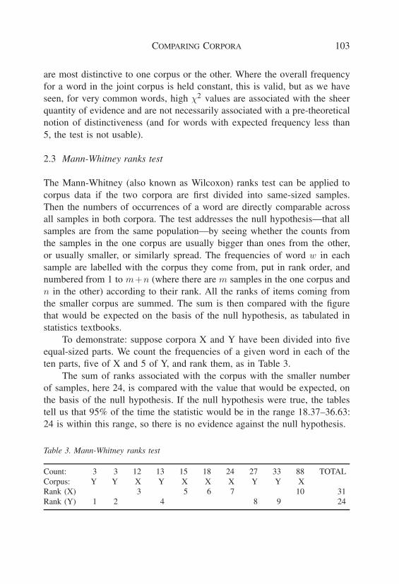
2.3 Mann-Whitney ranks test

The Mann-Whitney (also known as Wilcoxon) ranks test can be applied tocorpus data if the two corpora are first divided into same-sized samples.Then the numbers of occurrences of a word are directly comparable acrossall samples in both corpora. The test addresses the null hypothesis—that allsamples are from the same population—by seeing whether the counts fromthe samples in the one corpus are usually bigger than ones from the other,or usually smaller, or similarly spread. The frequencies of word w in eachsample are labelled with the corpus they come from, put in rank order, andnumbered from 1 to m+n (where there are m samples in the one corpus andn in the other) according to their rank. All the ranks of items coming fromthe smaller corpus are summed. The sum is then compared with the figurethat would be expected on the basis of the null hypothesis, as tabulated instatistics textbooks.

To demonstrate: suppose corpora X and Y have been divided into fiveequal-sized parts. We count the frequencies of a given word in each of theten parts, five of X and 5 of Y, and rank them, as in Table 3.

The sum of ranks associated with the corpus with the smaller numberof samples, here 24, is compared with the value that would be expected, onthe basis of the null hypothesis. If the null hypothesis were true, the tablestell us that 95% of the time the statistic would be in the range 18.37–36.63:24 is within this range, so there is no evidence against the null hypothesis.

Table 3. Mann-Whitney ranks test

Count: 3 3 12 13 15 18 24 27 33 88 TOTALCorpus: Y Y X Y X X X Y Y XRank (X) 3 5 6 7 10 31Rank (Y) 1 2 4 8 9 24

104 ADAM KILGARRIFF

Note that the one very high count of 88 has only limited impact onthe statistic. This is the desired behaviour for our task, since it is of limitedinterest if a single document in a corpus has very many occurrences of a word.

Sections 6.1 and 6.2 describe the use of rank-based statistics to findcharacteristic words in LOB vs. Brown, and in male vs. female speech.

2.4 t-test

The (unrelated) t-test, which operates on counts rather than on rank order ofcounts, could also be applied to frequency counts from two corpora dividedinto same-size samples. However the t-test is only valid where the data isnormally distributed, which is not in general the case for word counts (see be-low). The Mann-Whitney test has the advantage of being non-parametric, thatis, making no assumptions about the data obeying any particular distribution.

2.5 Mutual information

Another approach uses the Mutual Information (MI) statistic (Church andHanks 1989). This simply takes the (log of the) ratio of the word’s relativefrequency in one corpus to its relative frequency in the joint corpus. In termsof Table 1:

MIw,X = log2

(a

a + c× N

a + b

)This is an information theoretic measure (with relative frequencies serv-

ing as maximum likelihood estimators for probabilities) as distinct from onebased in statistical hypothesis testing, and it makes no reference to hypothe-ses. Rather, it states how much information word w provides about corpus X(with respect to the joint corpus). It was introduced into language engineeringas a measure for co-occurrence, where it specifies the information one wordsupplies about another.5

Church and Hanks state that MI is invalid for low counts, suggestinga threshold of 5. In contrast to χ2, there is no notion in MI of evidenceaccumulating. MI, for our purposes, is a relation between two corpora and aword: if the corpora are held constant, it is usually rare words which give thehighest MI. This contrasts with common words tending to have the highestχ2 scores. Church and Hanks proposed MI as a tool to help lexicographersisolate salient co-occurring terms. Several years on, it is evident that MI


overemphasises rare terms, relative to lexicographers’ judgements of salience,while χ2 correspondingly overemphasises common terms.

2.6 Log-likelihood (G2)

Dunning (1993) is concerned at the invalidity of both χ2 and MI wherecounts are low. The word he uses is ‘surprise’; he wants to quantify howsurprising various events are. He points out that rare events, such as theoccurrence of many words and most bigrams in almost any corpus, play alarge role in many language engineering tasks yet in these cases both MI andχ2 statistics are invalid. He then presents the log-likelihood statistic, whichgives an accurate measure of how surprising an event is even where it hasoccurred only once. For our contingency table, it can be calculated as:

G2=2(a log(a) + b log(b) + c log(c) + d log(d)−(a+ b) log(a + b) − (a + c) log(a + c)−(b+ d) log(b + d) − (c + d) log(c + d)+(a+ b + c + d) log(a + b + c + d))

Daille (1995) determines empirically that it is an effective measure forfinding terms. In relation to our simple case, of finding the most surpris-ingly frequent words in a corpus without looking at the internal structure ofthe corpus, G2 is a mathematically well-grounded and accurate measure ofsurprisingness, and early indications are that, at least for low and mediumfrequency words such as those in Daille’s study, it corresponds reasonablywell to human judgements of distinctiveness.6

2.7 Fisher’s exact test

Pedersen (1996) points out that log-likelihood approximates the probability ofthe data having occurred, given the null hypothesis, while there is a methodfor calculating it exactly: Fisher’s Exact method. The machinery for comput-ing it is available on various mathematical statistics packages. For very lowcounts, there is significant divergence between log-likelihood and the exactprobability.

106 ADAM KILGARRIFF

2.8 TF.IDF

The question, “Which words are particularly characteristic of a text?” is atthe heart of information retrieval (IR). These are the words which will bethe most appropriate key words and search terms. The general IR problemis to retrieve just the documents which are relevant to a user’s query, from adatabase of many documents.7

A very simple method would be to recall just those documents containingone or more of the search terms. Since the user does not want to be swampedwith ‘potentially relevant’ documents, this method is viable only if none ofthe search terms occur in many documents. Also, one might want to rank thedocuments, putting those containing more of the search terms at the top of thelist. This suggests two modifications to the very simple method which giveus the widely-used TF.IDF (term frequency by inverse document frequency)statistic (Salton 1989: 280 and references therein). Firstly a search term isof more value, the fewer documents it occurs in: IDF (inverse documentfrequency) is calculated, for each term in a collection, as the log of theinverse of the proportion of documents it occurs in. Secondly, a term is morelikely to be important in a document, the more times it occurs in it: TF fora term and a document is simply the number of times the term occurs in thedocument.

Now, rather than simply registering a hit if there are any matches betweena query term and a term in a document, we accumulate the TF.IDF scores foreach match. We can then rank the hits, with the documents with the highestsummed TF.IDF coming at the top of the list. This has been found to be asuccessful approach to retrieval (Robertson and Sparck Jones 1994).8

Two considerations regarding this scheme are:

• As described so far, it does not normalise for document length.In IR applications, TF is usually normalised by the length of thedocument. The discussion above shows that this is not altogethersatisfactory. A single use of a word in a hundred-word document isfar less noteworthy than ten uses of the word in a thousand-worddocument, but, if we normalise TF, they become equivalent.

• Very common words will be present in all documents. In this case,IDF = log 1 = 0 and TF.IDF collapses to zero. This point is not ofparticular interest to IR, as IR generally puts very common words


on a stop list and ignores them, but it is a severe constraint on thegenerality of TF.IDF.

3. Probability distributions for words

As Church and Gale (1995) say, words come in clumps; unlike lightening,they often strike twice. Where a word occurs once in a text, you are sub-stantially more likely to see it again than if it had not occurred once. Oncea corpus is seen as having internal structure—that is, comprising distincttexts—the independence assumption is unsustainable.

Some words are ‘clumpier’ or ‘burstier’ than others; typically contentwords are clumpier than grammatical words. The ‘clumpiness’ or ‘burstiness’of a particular word is an aspect of its behaviour which is important for manylanguage-engineering and linguistic purposes, and in this section we sketchvarious approaches to modelling and measuring it.

The three probability distributions which are most commonly cited in theliterature are the poisson, the binomial, and the normal. (Dunning refers to themultinomial, but for current purposes this is equivalent to the binomial.) Thenormal distribution is most often used as a convenient approximation to thebinomial or poisson, where the mean is large, as justified by the Central LimitTheorem. For all three cases (poisson, binomial, or normal approximating toeither) the distribution has just one parameter. Mean and variance do notvary independently: for the poisson they are equal, and for the binomial, ifthe expected value of the mean is p, the expected value of the variance isp(1 − p).

To relate this to word-counting, consider the situation in which thereare a number of same-length text samples. If words followed a poisson orbinomial distribution then if a word occurred, on average, c times in a sample,the expected value for the variance of hits-per-sample is also c (or, in thebinomial case, slightly less: the difference is negligible for all but the mostcommon words). As various authors have found, this is not the case. Mostof the time, the variance is greater than the mean. This was true for all buttwo of the 5,000 most common words in the BNC.9

108 ADAM KILGARRIFF

3.1 Poisson mixtures

Following Mosteller and Wallace (1964), Gale and Church identify Poissonmodels as belonging to the right family of distributions for describing wordfrequencies, and then generalise so that the single poisson parameter is itselfvariable and governed by a probability distribution. A ‘poisson mixture’ dis-tribution can then be designed with parameters set in such a way that, for aword of a given level of clumpiness and overall frequency in the corpus, thetheoretical distribution models the number of documents it occurs in and thefrequencies it has in those documents.

They list a number of ways in which clumping—or, more technically,‘deviation from poisson’—can be measured. IDF is one, variance another,and they present three more. These empirical measures of clumpiness canthen be used to set the second parameter of the poisson-mixture probabilitymodel. They show how these improved models can be put to work within aBayesian approach to author identification.

3.2 TERMIGHT and Katz’s model

Justeson and Katz (1995) and Katz (1996) present a more radical account ofword distributions. The goal of their TERMIGHT system was to identify andindex all the terms worth indexing in a document collection. They note thesimple fact that a topical term—a term denoting what a document or partof a document was about—occurs repeatedly in documents about that topic.TERMIGHT identifies terms by simply finding all those words and phrases ofthe appropriate syntactic shape (noun phrases without subordinate clauses)which occur more than once in a document. Katz (1996) takes the themefurther. He argues that word frequencies are not well modelled unless wetake into account the linguistic intuition that a document is or is not about atopic, and that that means documents will tend to have zero occurrences of aterm, or multiple occurrences. For terms, documents containing exactly oneoccurrence of a term will not be particularly common. Katz models wordprobability distributions with three parameters: first, the probability that itoccurs in a document at all (document frequency), second, the probabilitythat it will occur a second time in a document given that it has occurredonce, and third, the probability that it will occur another time, given thatit has already occurred k times (where k > 1). Thus the first parameter


(which is most closely related to the pre-theoretical idea of a word being inmore or less common usage) is independent of the second and third (whichaddress how term-like the word is). Katz argues that, for true terms, the thirdparameter is very high, approaching unity: where a term has already occurredtwice or more in a document, it is the topic of the document, so we shouldnot be surprised if it occurs any number of further times.

Katz establishes that his model provides a closer fit to corpus data thana number of other models for word distributions that have been proposed,including Poisson mixtures.

3.3 Adjusted frequencies

The literature includes some proposals that word counts for a corpus shouldbe adjusted to reflect clumpiness, with a word’s frequency being adjusteddownwards, the clumpier it is. The issues are described in Francis and Kucera(1982: 461–464). Francis and Kucera use a measure they call AF, attributed(indirectly) to J. Lanke of Lund University. It is defined as:

AF =

(n∑

i=1

(dixi)12

)2

where the corpus is divided into n categories (which could be texts but, inFrancis and Kucera’s analysis, are genres, each of which contain numeroustexts); di is the proportion of the corpus in that category; and xi is the countfor the word in the category.

Adjusting frequencies is of importance where the rank order is to be useddirectly for some purpose, for example, for choosing vocabulary for language-teaching, or in other circumstances where a single-parameter account of aword’s distribution is wanted. Here, I mention it for purposes of completeness.A two- or three-parameter model as proposed by Church and Gale or Katzgives a more accurate picture of a word’s behaviour than any one-parametermodel.

110 ADAM KILGARRIFF

4. Summary statistics for human interpretation

4.1 Content analysis

Content analysis is the social science tradition of quantitative analysis oftexts to determine themes. It was particularly popular in the 1950s and 60s,a landmark being the General Enquirer (Stone et al. 1966), an early comput-erised system. Studies using the method have investigated a great range oftopics, from analyses of propaganda and of changes in the tone of politicalcommuniques over time, to psychotherapeutic interviews and the social psy-chology of interactions between management, staff and patients in nursinghomes. The approach is taught in social science ‘methods’ courses, and usedin political science (Fan 1988), psychology (Smith 1992) and market research(Wilson and Rayson 1993). The basic method is to:

• identify a set of ‘concepts’ which words might fall into, on the basisof a theoretical understanding of the situation;

• classify words into these concepts, to give a content analysis dic-tionary;

• take the texts (these will often be transcribed spoken material);

• for each text, count the number of occurrences of each concept.

One recent scheme, Minnesota Contextual Content Analysis (McTavishand Pirro 1990, MCCA), uses both a set of 116 concepts and an additional,more general level of 4 ‘contexts’. Norms for levels of usage of each conceptcome with the MCCA system, and scores for each concept are defined bytaking the difference between the norm and the count for each concept-textpair (and dividing by the standard deviation of the concept across contexts).The concept scores are then directly comparable, between concepts and be-tween texts. The approach is primarily descriptive: it provides a new way ofdescribing texts, which it is then for the researcher to interpret and explain,so MCCA does nothing more with the concept scores.

It does however also provide the context scores. These serve severalpurposes, including

[to] contribute to a kind of “triangulation”, which would help to locate anypotential text in relation to each of the “marker” contexts. (p. 250)


The validity of this kind of analysis is to be found in its predictive power.A content analysis study of open-ended conversations between husbands andwives was able to classify the couples as ‘seeking divorce’, ‘seeking outsidehelp’, or ‘coping’ (McDonald and Weidetke 1979, quoted in McTavish andPirro: 260).

4.2 Multi-dimensional analysis

A major goal of sociolinguistics is to identify the main ways in which lan-guage varies, from group to group and context to context. Biber (1988 and1995) identifies the main dimensions of variation for English and three otherlanguages using the following method:

• Gather a set of text samples to cover a wide range of languagevarieties;

• Enter them (“the corpus”) into the computer;

• Identify a set of linguistic features which are likely to serve asdiscriminators for different varieties;

• Count the number of occurrences of each linguistic feature in eachtext sample;

• Perform a factor analysis (a statistical procedure) to identify whichlinguistic features tend to co-occur in texts. The output is a setof “dimensions”, each of which carry a weighting for each of thelinguistic features;

• Interpret each dimension, to identify what linguistic features, andwhat corresponding communicative functions, high-positive andhigh-negative values on the dimension correspond to.

For English, Biber identifies seven dimensions, numbered in decreasing or-der of significance (so dimension 1 accounts for the largest part of the non-randomness of the data, dimension 2, the next largest, etc.) The first hecalls “Involved versus Informational Production”. Texts getting high positivescores are typically spoken and typically conversations. Texts getting highnegative scores are academic prose and official documents. The linguisticfeatures with the highest positive weightings are “private” verbs (assume,believe etc.), that-deletion, contractions, present tense verbs, and second per-son pronouns. The linguistic features with the highest negative weightings are

112 ADAM KILGARRIFF

nouns, word length, prepositions, and type-token ratio. The two books citedabove present the case for the explanatory power of the multidimensionalapproach.

Any text can be given a score for any dimension, by counting the num-bers of occurrences of the linguistic features in the text, weighting, and sum-ming. The approach offers the possibility of “triangulation”, placing a textwithin the space of English language variation, in a manner comparable toMCCA’s context scores but using linguistic rather than social-science con-structs, and using a statistical procedure rather than theory to identify thedimensions.

The methods described in Section 2 all take each word as a distinctdata point, so each word defines a distinct dimension of a vector describingthe differences. Biber first reduces the dimensionality of the space to a levelwhere it is manageable by a human, and then offers contrasts between texts,and comments about what is distinctive about a text, in terms of these sevendimensions.10 He thereby achieves some generalisation: he can describe howclasses of features behave, whereas the other methods can only talk aboutthe behaviour of individual words.

5. Discussion

Clearly, people working in the area of measuring what is distinctive about atext have had a variety of goals. Some have been producing figures primarilyfor further automatic manipulation, others have had human scrutiny in mind.Some have been comparing texts with texts, others, texts or corpora withcorpora, and others again have been making comparisons with norms for thelanguage at large. Some (Biber, Mosteller and Wallace) have looked moreclosely at high-frequency, form words; others (McTavish and Pirro, Dunning,Church and Gale) at medium and low frequency words.

The words in a corpus approximate to a Zipfian distribution, in which theproduct of rank order and frequency is constant. So, to a first approximation,the most common word in a corpus is a hundred times as common as thehundredth most common, a thousand times as common as the thousandth,and a million times as common as the millionth. This is a very skeweddistribution. The few very common words have several orders of magnitudemore occurrences than most others. The different ends of the range tend


to have very different statistical behaviour. Thus, as we have seen, high-frequency words tend to give very high χ2 error terms whereas very highMI scores come from low-frequency words. Variance, as we have seen, isalmost always greater than the mean, and the ratio tends to increase withword frequency.

Linguists have long made a distinction approximating to the high/lowfrequency contrast: form words (or ‘grammar words’ or ‘closed class words’)vs. content words (or ‘lexical words’ or ‘open class words’). The relationbetween the distinct linguistic behaviour, and the distinct statistical behaviourof high-frequency words is obvious yet intriguing.

It would not be surprising if we cannot find a statistic which works wellfor both high and medium-to-low frequency words. It is far from clear whata comparison of the distinctiveness of a very common word and a rare wordwould mean.

6. Finding words that vary across text-type: experiments

In this section I describe two experiments in which the Mann-Whitney rankstest is used to find words that are systematically used more in one text typethan another.

6.1 LOB-Brown comparison

The LOB and Brown corpora both contain 2,000-word-long texts, so thenumbers of occurrences of a word are directly comparable across all samplesin both corpora. Had all 500 texts from each of LOB and Brown been usedas distinct samples for the purposes of the ranks test, most counts wouldhave been zero for all but very common words and the test would have beeninapplicable. To make it applicable, it was necessary to agglomerate textsinto larger samples. Ten samples for each corpus were used, each samplecomprising 50 texts and 100,000 words. Texts were randomly assigned toone of these samples (and the experiment was repeated ten times, to givedifferent random assignments, and the results averaged.) Following someexperimentation, it transpired that most words with a frequency of 30 ormore in the joint LOB and Brown had few enough zeroes for the test to beapplicable, so tests were carried out for just those words, 5,733 in number.

114 ADAM KILGARRIFF

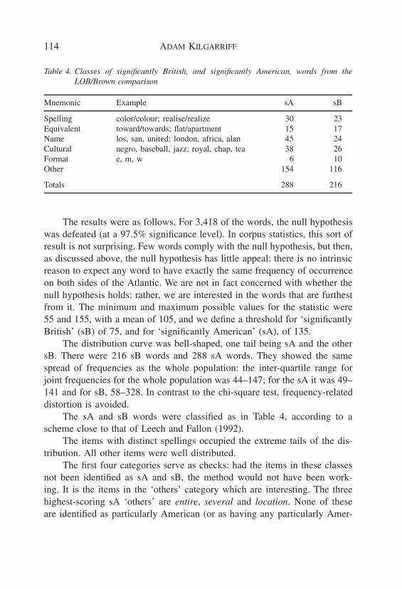
Table 4. Classes of significantly British, and significantly American, words from theLOB/Brown comparison

Mnemonic Example sA sB

Spelling color/colour; realise/realize 30 23Equivalent toward/towards; flat/apartment 15 17Name los, san, united; london, africa, alan 45 24Cultural negro, baseball, jazz; royal, chap, tea 38 26Format e, m, w 6 10Other 154 116

Totals 288 216

The results were as follows. For 3,418 of the words, the null hypothesiswas defeated (at a 97.5% significance level). In corpus statistics, this sort ofresult is not surprising. Few words comply with the null hypothesis, but then,as discussed above, the null hypothesis has little appeal: there is no intrinsicreason to expect any word to have exactly the same frequency of occurrenceon both sides of the Atlantic. We are not in fact concerned with whether thenull hypothesis holds: rather, we are interested in the words that are furthestfrom it. The minimum and maximum possible values for the statistic were55 and 155, with a mean of 105, and we define a threshold for ‘significantlyBritish’ (sB) of 75, and for ‘significantly American’ (sA), of 135.

The distribution curve was bell-shaped, one tail being sA and the othersB. There were 216 sB words and 288 sA words. They showed the samespread of frequencies as the whole population: the inter-quartile range forjoint frequencies for the whole population was 44–147; for the sA it was 49–141 and for sB, 58–328. In contrast to the chi-square test, frequency-relateddistortion is avoided.

The sA and sB words were classified as in Table 4, according to ascheme close to that of Leech and Fallon (1992).

The items with distinct spellings occupied the extreme tails of the dis-tribution. All other items were well distributed.

The first four categories serve as checks: had the items in these classesnot been identified as sA and sB, the method would not have been work-ing. It is the items in the ‘others’ category which are interesting. The threehighest-scoring sA ‘others’ are entire, several and location. None of theseare identified as particularly American (or as having any particularly Amer-


ican uses) in any of four 1995 learners’ dictionaries of English (LDOCE3,OALDCE5, CIDE, COBUILD2) all of which claim to cover both varietiesof the language. Of course it does not follow from the frequency differencethat there is a semantic or other difference that a dictionary should men-tion, but the ‘others’ list does provide a list of words for which linguists orlexicographers might want to examine whether there is some such difference.

6.2 Male/female conversation

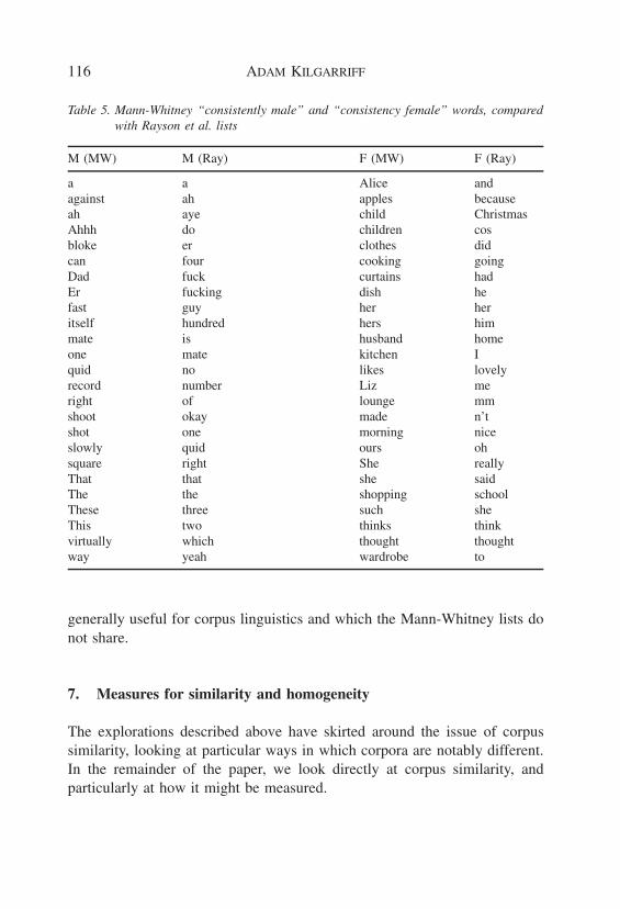
The spoken, conversational part of the BNC was based on a demographicsample of the UK population, sampled for age, gender, region and socialclass. It is a rich resource for investigating how speech varies across theseparameters. For details of its composition and collection see Crowdy (1993),Rayson, Leech, and Hodges (1997). Here we use it as a resource for exploringmale/female differences, and for contrasting lists of most different wordsgathered using χ2 with those gathered using the Mann-Whitney test.

Speaker turns where the gender of the speaker was available were iden-tified, giving two corpora, one of male speech (M), the other, of female (F).Each corpus was divided into 25,000-word chunks. The order of texts in theBNC was retained in M and F, and the chunking took, first, the first 25,000words, then the next 25,000, and so on, so the text relating to a single con-versation would never be found in more than two chunks. The organisationof the BNC also ensured that a single speaker’s words were unlikely to occurin more than two chunks. There were 31 M chunks and 50 F chunks. Thesechunks were then randomly combined into 150,000 word ‘slices’, giving fiveM slices and eight F slices. For each word with frequency of 20 or greater inM and F combined, the frequency in each slice was calculated, frequencieswere ranked, and the Mann-Whitney statistic was calculated twice, once withthe M slice always given the higher rank in cases of ties, once with the F,and the average taken.

The 25 words which are most consistently more common in M and F arepresented in Table 5, alongside the equivalent lists from Rayson et al.11 Alllists have been alphabeticised, for ease of comparison. Of the 25 commonestwords in the joint corpus (unnormalised for case), twelve are in Rayson etal.’s lists, whereas just one (a) is in either of the Mann-Whitney lists. TheRayson et al. lists display a bias towards high-frequency items which is not

116 ADAM KILGARRIFF

Table 5. Mann-Whitney “consistently male” and “consistency female” words, comparedwith Rayson et al. lists

M (MW) M (Ray) F (MW) F (Ray)

a a Alice andagainst ah apples becauseah aye child ChristmasAhhh do children cosbloke er clothes didcan four cooking goingDad fuck curtains hadEr fucking dish hefast guy her heritself hundred hers himmate is husband homeone mate kitchen Iquid no likes lovelyrecord number Liz meright of lounge mmshoot okay made n’tshot one morning niceslowly quid ours ohsquare right She reallyThat that she saidThe the shopping schoolThese three such sheThis two thinks thinkvirtually which thought thoughtway yeah wardrobe to

generally useful for corpus linguistics and which the Mann-Whitney lists donot share.

7. Measures for similarity and homogeneity

The explorations described above have skirted around the issue of corpussimilarity, looking at particular ways in which corpora are notably different.In the remainder of the paper, we look directly at corpus similarity, andparticularly at how it might be measured.


What are the constraints on a measure for corpus similarity? The first issimply that its findings correspond to unequivocal human judgements. It mustmatch our intuition that, for instance, a corpus of syntax papers is more likeone of semantics papers than one of shopping lists. The constraint is key butis weak. Direct human intuitions on corpus similarity are not easy to come by,firstly, because large corpora, unlike coherent texts, are not the sorts of thingspeople read, so people are not generally in a position to have any intuitionsabout them. Secondly, a human response to the question, “how similar aretwo objects”, where those objects are complex and multi-dimensional, willthemselves be multi-dimensional: things will be similar in some ways anddissimilar in others. To ask a human to reduce a set of perceptions about thesimilarities and differences between two complex objects to a single figureis an exercise of dubious value.

This serves to emphasise an underlying truth: corpus similarity is com-plex, and there is no absolute answer to “is Corpus 1 more like Corpus 2than Corpus 3?”. All there are are possible measures which serve particularpurposes more or less well. Given the task of costing the customisation ofan NLP system, produced for one domain, to another, a corpus similaritymeasure is of interest insofar as it predicts how long the porting will take.It could be that a measure which predicts well for one NLP system, predictsbadly for another. It can only be established whether a measure correctlypredicts actual costs, by investigating actual costs.12

Having struck a note of caution, we now proceed on the hypothesis thatthere is a single measure which corresponds to pre-theoretical intuitions about‘similarity’ and which is a good indicator of many properties of interest—customisation costs, the likelihood that linguistic findings based on one corpusapply to another, etc. We would expect the limitations of the hypothesis toshow through at some point, when different measures are shown to be suitedto different purposes, but in the current situation, where there has been almostno work on the question, it is a good starting point.

7.1 Similarity and homogeneity

How homogeneous is a corpus? The question is both of interest in its ownright, and is a preliminary to any quantitative approach to corpus similarity.In its own right, because a sublanguage corpus, or one containing only aspecific language variety, has very different characteristics to a general cor-

118 ADAM KILGARRIFF

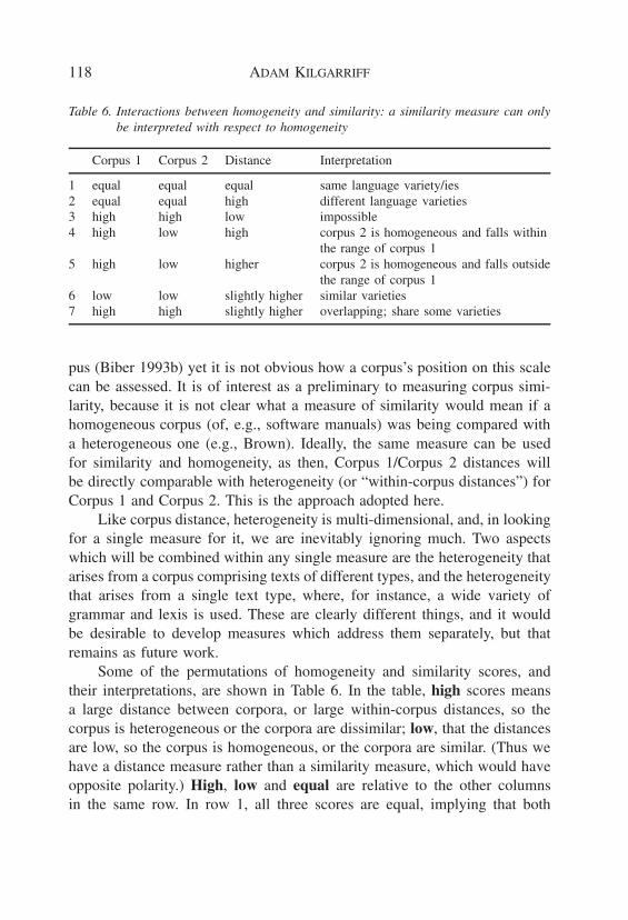
Table 6. Interactions between homogeneity and similarity: a similarity measure can onlybe interpreted with respect to homogeneity

Corpus 1 Corpus 2 Distance Interpretation

1 equal equal equal same language variety/ies2 equal equal high different language varieties3 high high low impossible4 high low high corpus 2 is homogeneous and falls within

the range of corpus 15 high low higher corpus 2 is homogeneous and falls outside

the range of corpus 16 low low slightly higher similar varieties7 high high slightly higher overlapping; share some varieties

pus (Biber 1993b) yet it is not obvious how a corpus’s position on this scalecan be assessed. It is of interest as a preliminary to measuring corpus simi-larity, because it is not clear what a measure of similarity would mean if ahomogeneous corpus (of, e.g., software manuals) was being compared witha heterogeneous one (e.g., Brown). Ideally, the same measure can be usedfor similarity and homogeneity, as then, Corpus 1/Corpus 2 distances willbe directly comparable with heterogeneity (or “within-corpus distances”) forCorpus 1 and Corpus 2. This is the approach adopted here.

Like corpus distance, heterogeneity is multi-dimensional, and, in lookingfor a single measure for it, we are inevitably ignoring much. Two aspectswhich will be combined within any single measure are the heterogeneity thatarises from a corpus comprising texts of different types, and the heterogeneitythat arises from a single text type, where, for instance, a wide variety ofgrammar and lexis is used. These are clearly different things, and it wouldbe desirable to develop measures which address them separately, but thatremains as future work.

Some of the permutations of homogeneity and similarity scores, andtheir interpretations, are shown in Table 6. In the table, high scores meansa large distance between corpora, or large within-corpus distances, so thecorpus is heterogeneous or the corpora are dissimilar; low, that the distancesare low, so the corpus is homogeneous, or the corpora are similar. (Thus wehave a distance measure rather than a similarity measure, which would haveopposite polarity.) High, low and equal are relative to the other columnsin the same row. In row 1, all three scores are equal, implying that both


corpora are of the same text type. In row 2, ‘equal’ in the first two columnsreads that the within-corpus distance (homogeneity) of Corpus 1 is roughlyequal to the within-corpus distance of Corpus 2, and ‘high’ in the Distancecolumn reads that the distance between the corpora is substantially higher thanthese within-corpus distances. Thus a comparison between the two corporais straightforward to interpret, since the two corpora do not differ radicallyin their homogeneity, and the outcome of the comparison is that they are ofmarkedly different language varieties.

Not all combinations of homogeneity and similarity scores are logicallypossible. For example, two corpora cannot be much more similar to eachother than either is to itself (row 3).

Rows 4 and 5 indicate two of the possible outcomes when a relativelyheterogeneous corpus (corpus 1) is compared with a relatively homogeneousone (corpus 2). It is not possible for the distance between the corpora to bemuch lower than the heterogeneity of the more heterogeneous corpus 1. Ifthe distance is roughly equal to corpus 1 heterogeneity, the interpretation isthat corpus 2 falls within the range of corpus 2; if it is higher, it falls outside.

The last two rows point to the differences between general corpora andspecific corpora. High and low values in the first two columns are to beinterpreted relative to norms for the language. Particularly high within-corpusdistance scores will be for general corpora, which embrace a number oflanguage varieties. Corpus similarity between general corpora will be a matterof whether all the same language varieties are represented in each corpus, andin what proportions. Low within-corpus distance scores will typically relateto corpora of a single language variety, so here, scores may be interpreted asa measure of the distance between the two varieties.

7.2 Related work

There is very little work which explicitly aims to measure similarity betweencorpora. The one clearly relevant item is Johansson anf Hofland (1989),which aims to find which genres, within the LOB corpus, most resembleeach other. They take the 89 most common words in the corpus, find theirrank within each genre, and calculate the Spearman rank correlation statistic(‘spearman’).

Rose, Haddock, and Tucker (1997) explore how performance of a speechrecognition system varies with the size and specificity of the training data

120 ADAM KILGARRIFF

used to build the language model. They have a small corpus of the target texttype, and experiment with ‘growing’ their seed corpus by adding more same-text-type material. They use Spearman and log-likelihood (Dunning 1993) asmeasures to identify same-text-type corpora. Spearman is evaluated below.

Sekine (1997) explores the domain dependence of parsing. He parsescorpora of various text genres and counts the number of occurrences of eachsubtree of depth one. This gives him a subtree frequency list for each corpus,and he is then able to investigate which subtrees are markedly differentin frequency between corpora. Such work is highly salient for customisingparsers for particular domains. Subtree frequencies could readily replace wordfrequencies for the frequency-based measures below.

In information-theoretic approaches, perplexity is a widely-used mea-sure. Given a language model and a corpus, perplexity “is, crudely speaking,a measure of the size of the set of words from which the next word is chosengiven that we observe the history of [. . . ] words” (Roukos 1996). Perplex-ity is most often used to assess how good a language modelling strategy is,so is used with the corpus held constant. Achieving low perplexity in thelanguage model is critical for high-accuracy speech recognition, as it meansthere are fewer high-likelihood candidate words for the speech signal to becompared with.

Perplexity can be used to measure a property akin to homogeneity if thelanguage modelling strategy is held constant and the corpora are varied. Inthis case, perplexity is taken to measure the intrinsic difficulty of the speechrecognition task: the less constraint the domain corpus provides on what thenext word might be, the harder the task. Thus Roukos (1996) presents atable in which different corpora are associated with different perplexities.Perplexity measures are evaluated below.

8. “Known-Similarity Corpora”

Proposing measures for corpus similarity is relatively straightforward: deter-mining which measures are good ones, is harder. To evaluate the measures,it would be useful to have a set of corpora where similarities were alreadyknown. In this section, we present a method for producing a set of “Known-Similarity Corpora” (KSC).


A KSC-set is built as follows: two reasonably distinct text types, A andB, are taken. Corpus 1 comprises 100% A; Corpus 2, 90% A and 10% B;Corpus 3, 80% A and 20% B; and so on. We now have at our disposal a setof fine-grained statements of corpus similarity: Corpus 1 is more like Corpus2 than Corpus 1 is like Corpus 3. Corpus 2 is more like Corpus 3 thanCorpus 1 is like Corpus 4, etc. Alternative measures can now be evaluated,by determining how many of these ‘gold standard judgements’ they get right.For a set of n Known-Similarity Corpora there are

n∑i=1

(n− i)

(i(i + 1)

2− 1

)

gold standard judgements (see Appendix 1 for proof) and the ideal measurewould get all of them right. Measures can be compared by seeing whatpercentage of gold standard judgements they get right.

Two limitations on the validity of the method are, first, there are differentways in which corpora can be different. They can be different because eachrepresents one language variety, and these varieties are different, or becausethey contain different mixes, with some of the same varieties. The methodonly directly addresses the latter model.

Second, if the corpora are small and the difference in proportions be-tween the corpora is also small, it is not clear that all the ‘gold standard’assertions are in fact true. There may be a finance supplement in one of thecopies of the Guardian in the corpus, and one of the copies of Accountancymay be full of political stories: perhaps, then, Corpus 3 is more like Corpus 5than Corpus 4. It is necessary to address this by selecting the two text typeswith care so they are similar enough so the measures are not all 100% cor-rect yet dissimilar enough to make it likely that all gold-standard judgementsare true, and by ensuring there is enough data and enough KSC-sets so thatoddities of individual corpora do not obscure the picture of the best overallmeasure.

9. Experiment to evaluate measures

We now describe an experiment in which KSC-sets were used to evaluatefour candidate measures for corpus similarity.

122 ADAM KILGARRIFF

9.1 The measures

All the measures use spelled forms of words. None make use of linguis-tic theories. The comment has been made that lemmas, or word senses, orsyntactic constituents, were more appropriate objects to count and performcomputations on than spelled forms. This would in many ways be desirable.However there are costs to be considered. To count, for example, syntacticconstituents requires, firstly, a theory of what the syntactic constituents are;secondly, an account of how they can be recognised in running text; andthirdly, a program which performs the recognition. Shortcomings or bugs inany of the three will tend to degrade performance, and it will not be straight-forward to allocate blame. Different theories and implementations are likelyto have been developed with different varieties of text in focus, so the degra-dation may well affect different text types differently. Moreover, practicalusers of a corpus-similarity measure cannot be expected to invest energy inparticular linguistic modules and associated theory. To be of general utility,a measure should be as theory-neutral as possible.

In these experiments we consider only raw word-counts. Two word fre-quency measures were considered. For each, the statistic did not dictate whichwords should be compared across the two corpora. In a preliminary investi-gation we had experimented with taking the most frequent 10, 20, 40 . . . 640,1280, 2560, 5120 words in the union of the two corpora as data points, andhad achieved the best results with 320 or 640. For the experiments below,we used the most frequent 500 words.

Both word-frequency measures can be directly applied to pairs of cor-pora, but only indirectly to measure homogeneity. To measure homogeneity:

1. divide the corpus into ‘slices’;

2. create two subcorpora by randomly allocating half the slices to each;

3. measure the similarity between the subcorpora;

4. iterate with different random allocations of slices;

5. calculate mean and standard deviation over all iterations.

Wherever similarity and homogeneity figures were to be compared, thesame method was adopting for calculating corpus similarity, with one sub-


corpus comprising a random half of Corpus 1, the other, a random half ofCorpus 2.

9.1.1 Spearman rank correlation co-efficientRanked wordlists are produced for Corpus 1 and Corpus 2. For each of the n

most common words, the difference in rank order between the two corporais taken. The statistic is then the normalised sum of the squares of thesedifferences,

1 − 6Σd2

n(n2 − 1)

9.1.2 CommentSpearman is easy to compute and is independent of corpus size: one candirectly compare ranked lists for large and small corpora. However the fol-lowing objection seemed likely to play against it. For very frequent words,a difference of rank order is highly significant: if the is the most commonword in corpus 1 but only third in corpus 2, this indicates a high degree ofdifference between the genres. But at the other end of the scale, the oppositeis the case: if bread is in 400th position in the one corpus and 500th in theother, this is of no significance; yet Spearman counts the latter as far moresignificant than the former.

χ2

For each of the n most common words, we calculate the number of oc-currences in each corpus that would be expected if both corpora were ran-dom samples from the same population. If the size of corpora 1 and 2 areN1,N2 and word w has observed frequencies ow,1, ow,2, then expected value

ew,1 =N1×(ow,1+ow,2)

N1+N2and ew,2 =

N2×(ow,1+ow,2)N1+N2

; then

χ2 = Σ(o− e)2

e

9.1.3 CommentThe inspiration for the statistic comes from the χ2-test for statistical inde-pendence. As shown above, the statistic is not in general appropriate forhypothesis-testing in corpus linguistics: a corpus is never a random sample

124 ADAM KILGARRIFF

of words, so the null hypothesis is of no interest. But once divested of thehypothesis-testing link, χ2 is suitable. The (o−e)2/e term gives a measure ofthe difference in a word’s frequency between two corpora, and the measuretends to increase slowly with word frequency in a way that is compatible withthe intuition that higher-frequency words are more significant in assessmentsof corpus similarity that lower-frequency ones.

The measure does not directly permit comparison between corpora ofdifferent sizes.

9.1.4 Perplexity and cross-entropyFrom an information-theoretic point of view, prima facie, entropy is a welldefined term capturing the informal notion of homogeneity, and the cross-entropy between two corpora captures their similarity. Entropy is not a quan-tity that can be directly measured. The standard problem for statistical lan-guage modelling is to aim to find the model for which the cross-entropy ofthe model for the corpus is as low as possible. For a perfect language model,the cross-entropy would be the entropy of the corpus (Church and Mercer1993, Charniak 1993).

With language modelling strategy held constant, the cross-entropy of alanguage model (LM) trained on Corpus 1, as applied to Corpus 2, is a sim-ilarity measure. The cross-entropy of the LM based on nine tenths of Corpus1, as applied to the other ‘held-out’ tenth, is a measure of homogeneity. Westandardised on the ‘tenfold cross-validation’ method for measures of bothsimilarity and homogeneity: that is, for each corpus, we divided the corpusinto ten parts13 and produced ten LMs, using nine tenths and leaving out adifferent tenth each time. (Perplexity is the log of the cross-entropy of a cor-pus with itself: measuring homogeneity as self-similarity is standard practicein information theoretic approaches.)

To measure homogeneity, we calculated the cross-entropy of each ofthese LMs as applied to the left-out tenth, and took the mean of the tenvalues. To measure similarity, we calculated the cross-entropy of each of theCorpus 1 LMs as applied to a tenth of Corpus 2 (using a different tenth eachtime). We then repeated the procedure with the roles of Corpus 1 and Corpus2 reversed, and took the mean of the 20 values.

All LMs were trigram models. All LMs were produced and calculationsperformed using the CMU/Cambridge toolkit (Rosenfeld 1995).


The treatment of words in the test material but not in the training ma-terial was critical to our procedure. It is typical in the language modellingcommunity to represent such words with the symbol UNK, and to calculatethe probability for the occurrence of UNK in the test corpus using one ofthree main strategies.

Closed vocabulary The vocabulary is defined to include all items in trainingand test data. Probabilities for those items that occur in training but nottest data, the ‘zerotons’, are estimated by sharing out the probability massinitially assigned to the singletons and doubletons to include the zerotons.

Open, type 1 The vocabulary is chosen independently of the training andtest data, so the probability of UNK may be estimated by counting theoccurrence of unknown words in the training data and dividing by N (thetotal number of words).

Open, type 2 The vocabulary is defined to include all and only the trainingdata, so the probability of UNK cannot be estimated directly from thetraining data. It is estimated instead using the discount mass created bythe normalisation procedure.

All three strategies were evaluated.

9.2 Data

All KSC sets were subsets of the British National Corpus (BNC). A numberof sets were prepared as follows.

For those newspapers or periodicals for which the BNC contained over300,000 running words of text, word frequency lists were generated andsimilarity and homogeneity were calculated (using χ2; results are shown inAppendix 2.) We then selected pairs of text types which were moderatelydistinct, but not too distinct, to use to generate KSC sets. (In initial experi-ments, more highly distinct text types had been used, but then both Spearmanand χ2 had scored 100%, so ‘harder’ tests involving more similar text typeswere selected.)

For each pair a and b, all the text in the BNC for each of a and b wasdivided into 10,000-word tranches. These tranches were randomly shuffledand allocated as follows:

126 ADAM KILGARRIFF

first 10 of a into b0anext 9 of a, first 1 of b into b1anext 8 of a, next 2 of b into b2anext 7 of a, next 3 of b into b3a. . .

until either the tranches of a or b ran out, or a complete eleven-corpus KSC-set was formed. A sample of KSC sets are available is the web.14 There were21 sets containing between 5 and 11 corpora. The method ensured that thesame piece of text never occurred in more than one of the corpora in a KSCset.

The text types used were:Accountancy (acc); The Art Newspaper (art); British Medical Journal(bmj); Environment Digest (env); The Guardian (gua); The Scotsman(sco); and Today (‘low-brow’ daily newspaper, tod).

To the extent that some text types differ in content, whereas others differin style, both sources of variation are captured here. Accountancy and The ArtNewspaper are both trade journals, though in very different domains, whileThe Guardian and Today are both general national newspapers, of differentstyles.

9.3 Results

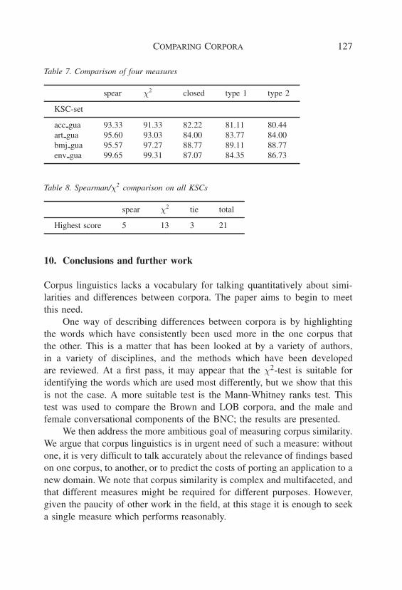
For each KSC-set, for each gold-standard judgement, the ‘correct answer’was known, e.g., “the similarity 1,2 is greater than the similarity 0,3”. Agiven measure either agreed with this gold-standard statement, or disagreed.The percentage of times it agreed is a measure of the quality of the measure.Results for the cases where all four measures were investigated are presentedin Table 7.

The word frequency measures outperformed the perplexity ones. It isalso salient that the perplexity measures required far more computation: ca.12 hours on a Sun, as opposed to around a minute.

Spearman and χ2 were tested on all 21 KSC-sets, and χ2 performedbetter for 13 of them, as shown in Table 8.

The difference was significant (related t-test: t = 4.47, 20DF, significantat 99.9% level). χ2 was the best of the measures compared.


Table 7. Comparison of four measures

spear χ2 closed type 1 type 2

KSC-set

acc gua 93.33 91.33 82.22 81.11 80.44art gua 95.60 93.03 84.00 83.77 84.00bmj gua 95.57 97.27 88.77 89.11 88.77env gua 99.65 99.31 87.07 84.35 86.73

Table 8. Spearman/χ2 comparison on all KSCs

spear χ2 tie total

Highest score 5 13 3 21

10. Conclusions and further work

Corpus linguistics lacks a vocabulary for talking quantitatively about simi-larities and differences between corpora. The paper aims to begin to meetthis need.

One way of describing differences between corpora is by highlightingthe words which have consistently been used more in the one corpus thatthe other. This is a matter that has been looked at by a variety of authors,in a variety of disciplines, and the methods which have been developedare reviewed. At a first pass, it may appear that the χ2-test is suitable foridentifying the words which are used most differently, but we show that thisis not the case. A more suitable test is the Mann-Whitney ranks test. Thistest was used to compare the Brown and LOB corpora, and the male andfemale conversational components of the BNC; the results are presented.

We then address the more ambitious goal of measuring corpus similarity.We argue that corpus linguistics is in urgent need of such a measure: withoutone, it is very difficult to talk accurately about the relevance of findings basedon one corpus, to another, or to predict the costs of porting an application to anew domain. We note that corpus similarity is complex and multifaceted, andthat different measures might be required for different purposes. However,given the paucity of other work in the field, at this stage it is enough to seeka single measure which performs reasonably.

128 ADAM KILGARRIFF

The Known-Similarity Corpora method for evaluating corpus-similaritymeasures was presented, and measures discussed in the literature were com-pared using it. For the corpus-size used and this approach to evaluation, χ2

and Spearman both performed better than any of three cross-entropy mea-sures. These measures have the advantage that they are cheap and straight-forward to compute. χ2 outperformed Spearman.

Thus χ2 is presented as a suitable measure for comparing corpora, andis shown to be the best measure of those tested. It can be used for measuringthe similarity of a corpus to itself, as well as the similarity of one corpus toanother, and this feature is valuable as, without self-similarity as a point ofreference, a measure of similarity between corpora is uninterpretable.

There are, naturally, some desiderata it does not meet. Unlike cross-entropy, it is not rooted in a mathematical formalism which provides theprospect of integrating the measure with some wider theory. Also, an idealmeasure would be scale-independent, supporting the comparison of small andlarge corpora. This is an area for future work.

Acknowledgements

This work has been supported by the EPSRC, Grants K18931 and M54971and a Macquarie University Research Grant. I am particularly grateful toTony Rose, who undertook the language modelling and cross-entropy calcu-lations. The work has also benefited from comments from Harald Baayen,Ted Dunning and Mark Lauer.

Appendix 1

The proof is based on the fact that the number of similarity judgements isthe triangle number of the number of corpora in the set (less one), and thateach new similarity judgement introduces a triangle number of gold standardjudgements (once an ordering which rules out duplicates is imposed on goldstandard judgements).

• A KSC set is ordered according to the proportion of text of type 1.Call the corpora in the set 1 . . . n.


• A similarity judgement (‘sim’) between a and b (a, b) compares twocorpora. To avoid duplication, we stipulate that a < b. Each sim isassociated with a number of steps of difference between the corpora:dif(a, b) = b− a.

• A gold standard judgement (‘gold’) compares two sims; there isonly a gold between a, b and c, d if a < b and c < d (as stipulatedabove) and also if a <= c, b >= d, and not (a = c and b = d).Each four-way comparison can only give rise to zero or one gold,as enforced by the ordering constraints. Each gold has a differenceof difs (‘difdif’) of (b − a) − (d − c) (so, if we compare 3, 5 with3, 4, difdif = 1, but where we compare 2, 7 with 3, 4, difdif = 4).difdif(X ,Y ) = dif(X) − dif(Y ).

• Adding an nth corpus to a KSC set introduces n − 1 sims. Theirdifs vary from 1 (for (n− 1),n) to n− 1 (for 1,n).

• The number of golds with a sim of dif m as first term is a trianglenumber less one,

∑mi=2 i or m(m+1)

2 −1. For example, for 2, 6 (dif =

4) there are 2 golds of difdif 1 (e.g. with 2, 5 and 3, 6), 3 of difdif2 (with 2, 4, 3, 5, 4, 6), and 4 of difdif 3 (with 2, 3, 3, 4, 4, 5, 5, 6).

• With the addition of the nth corpus, we introduce n− 1 sims withdifs from 1 to n−1, so we add

∑n−1i=1

i(i+1)2 −1 golds. For the whole

set, there are∑n

i=1∑i−1

j=1j(j+1)

2 −1 and collecting up repeated terms

gives∑n

i=1(n− i)( i(i+1)2 − 1)

Appendix 2

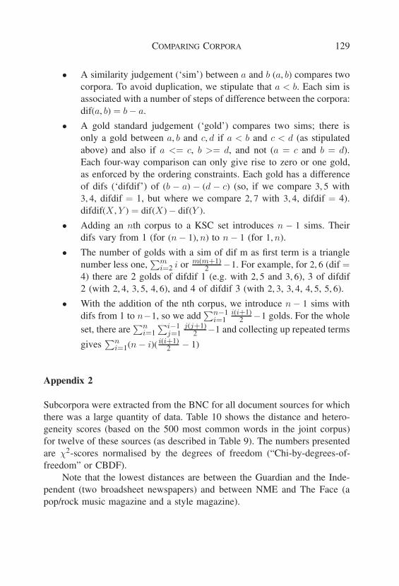
Subcorpora were extracted from the BNC for all document sources for whichthere was a large quantity of data. Table 10 shows the distance and hetero-geneity scores (based on the 500 most common words in the joint corpus)for twelve of these sources (as described in Table 9). The numbers presentedare χ2-scores normalised by the degrees of freedom (“Chi-by-degrees-of-freedom” or CBDF).

Note that the lowest distances are between the Guardian and the Inde-pendent (two broadsheet newspapers) and between NME and The Face (apop/rock music magazine and a style magazine).

130 ADAM KILGARRIFF

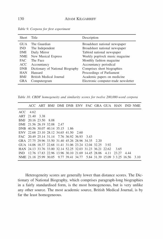
Table 9. Corpora for first experiment

Short Title Description

GUA The Guardian Broadsheet national newspaperIND The Independent Broadsheet national newspaperDMI Daily Mirror Tabloid national newspaperNME New Musical Express Weekly pop/rock music magazineFAC The Face Monthly fashion magazineACC Accountancy Accountancy periodicalDNB Dictionary of National Biography Comprises short biographiesHAN Hansard Proceedings of ParliamentBMJ British Medical Journal Academic papers on medicineGRA Computergram Electronic computer-trade newsletter

Table 10. CBDF homogeneity and similarity scores for twelve 200,000-word corpora

ACC ART BMJ DMI DNB ENV FAC GRA GUA HAN IND NME

ACC 4.62ART 21.40 3.38BMJ 20.16 23.50 8.08DMI 21.56 26.19 32.08 2.47DNB 40.56 30.07 40.14 35.15 1.86ENV 22.68 23.10 28.12 34.65 41.50 2.60FAC 20.49 25.14 31.14 7.76 36.92 36.93 3.43GRA 27.75 29.96 33.50 31.40 45.26 28.96 34.35 2.20GUA 14.06 18.37 22.68 11.41 31.06 23.24 12.04 32.25 3.92HAN 24.13 33.76 33.00 32.14 52.25 32.03 31.23 36.21 22.62 3.65IND 12.76 17.83 22.96 13.96 30.10 21.69 14.45 28.06 4.11 23.27 4.44NME 21.18 25.99 30.05 9.77 39.41 34.77 5.84 31.39 15.09 3 3.25 16.56 3.10

Heterogeneity scores are generally lower than distance scores. The Dic-tionary of National Biography, which comprises paragraph-long biographiesin a fairly standardised form, is the most homogeneous, but is very unlikeany other source. The most academic source, British Medical Journal, is byfar the least homogeneous.


Notes

1. Alternative names for the field (or a closely related one) are “empirical linguistics” and“data-intensive linguistics”. By using an adjective rather than a noun, these seem not toassert that the corpus is an object of study. Perhaps it is equivocation about what we cansay about corpora that has led to the coining of the alternatives.

2. Provided all expected values are over a threshold of 5.

3. See http://info.ox.ac.uk/bnc

4. In this case the null hypothesis is true, so the average value of the sum of the errorterms over the four cells of the contingency table is 1 (from the definition of the χ2

distribution). Of the four cells, the two error-terms associated with the absence of theword (cells c and d in Table 1) will be vanishingly small, as E is large —almost as largeas the number of words in the corpus—whereas (|O−E|−0.5)2 is small, so the result ofdividing it by E is vanishingly small. The two cells corresponding to the presence of theword (cells a and b in Table 1) will both have the same average value, since, by design,the two corpora are the same size. Thus the four-way sum is effectively shared betweencells a and b, so the average value of each is 0.5.

5. The usage of the term “mutual information” within information theory is different:MI(X;Y ) = Σx,y log p(x,y)

p(x)p(y) . However, in language engineering, the Church-Hanks de-finition has been widely adopted so here, MI will refer to that simpler term.

6. Several corpus interface packages provide functionality for computing one or more ofthese statistics. For example, WordSmith (Scott 1997 and Sardinha 1996) and the associ-ated KeyWords tool allows the user to generate lists using Mutual Information, chi-squareand log-likelihood.

7. We assume full-text searching. Also, issues such as stemming and stop lists are notconsidered, as they do not directly affect the statistical considerations.

8. They also provide a ‘tuning constant’ for adjusting the relative weight given to TF andIDF to optimise performance.

9. Figures based on the standard-document-length subset of the BNC described above.

10. Reducing the dimensionality of the problem has also been explored in IR: see Schutzeand Pederson (1995), Dumais et al. (1988).

11. Rayson et al. The comparisons are normalised for case, so this is one point at whichdirect comparison is not possible.

12. Cf. Ueberla (1997), who looks in detail at the appropriateness of perplexity as a measureof task difficulty for speech recognition, and finds it wanting.

13. For the KSC corpora, we ensured that each tenth had an appropriate mix of text types,so that, e.g. each tenth of a corpus comprising 70% Guardian, 30% BMJ, also comprised70% Guardian, 30% BMJ.

14. http://www.itri.bton.ac.uk/ Adam.Kilgarriff/KSC/

132 ADAM KILGARRIFF

References

Biber, D. 1988. Variation across speech and writing. Cambridge: Cambridge UniversityPress.

Biber, D. 1990. “Methodological issues regarding corpus-based analyses of linguisticvariation.” Literary and Linguistic Computing 5: 257–269.

Biber, D. 1993a. “Representativeness in corpus design.” Literary and LinguisticComputing 8: 243–257.

Biber, D. 1993b. “Using register-diversified corpora for general language studies.”Computational Linguistics 19(2): 219–242.

Biber, D. 1995. Dimensions in Register Variation. Cambridge: Cambridge UniversityPress.

Charniak, E. 1993. Statistical Language Learning. Cambridge, Mass, MIT Press.Church, K. and W. Gale. 1995. “Poisson mixtures.” Journal of Natural Language

Engineering 1(2): 163–190.Church, K. and P. Hanks. 1989. “Word association norms, mutual information and

lexicography.” ACL Proceedings, 27th Annual Meeting, 76–83. Vancouver: ACL.Church, K. W. and R. L. Mercer. 1993. “Introduction to the special issue on computational

linguistics using large corpora.” Computational Linguistics 19(1): 1–24.Crowdy, S. 1993. “Spoken corpus design.” Literary and Linguistic Computing 8: 259–

265.Daille, B. 1995. Combined approach for terminology extraction: lexical statistics and

linguistic filtering. Technical Report 5. Lancaster University: UCREL.Dumais, S., G. Furnas, T. Landauer, S. Deerwester, and R. Harshman. 1988. “Using latent

semantic analysis to improve access to textual information.” Proceedings of CHI ’88,281–285. Washington DC: ACM.

Dunning, T. 1993. “Accurate methods for the statistics of surprise and coincidence.”Computational Linguistics 19(1): 61–74.

Fan, D. P. 1988. Predictions of public opinion from the mass media: computer contentanalysis and mathematical modeling. New York: Greenwood Press.

Francis, W. N. and H. Kucera. 1982. Frequency Analysis of English Usage: lexicon andgrammar. Boston: Houghton Mifflin.

Hofland, K. and S. Johansson (eds). 1982. Word Frequencies in British and AmericanEnglish. Bergen: The Norwegian Computing Centre for the Humanities.

Johansson, S. and K. Hofland (eds). 1989. Frequency Analysis of English vocabularyand grammar, based on the LOB corpus. Oxford: Clarendon.

Justeson, J. S. and S. M. Katz. 1995. “Technical terminology: some linguistic propertiesand an algorithm for identification in text.” Natural Language Engineering 1(1): 9–27.

Katz, S. 1996. “Distribution of content words and phrases in text and languagemodelling.” Natural Language Engineering 2(1): 15–60.

Leech, G. and R. Fallon. 1992. “Computer corpora—what do they tell us about culture?”ICAME Journal 16: 29–50.

McDonald, C. and B. Weidetke. 1979. Testing marriage climate. Masters thesis. Ames,Iowa: Iowa State University.


McTavish, D. G. and E. B. Pirro. 1990. “Contextual content analysis.” Quality andQuantity 24: 245–265.

Mosteller, F. and D. L. Wallace. 1964. Applied Bayesian and Classical Inference—TheCase of The Federalist Papers. Springer Series in Statistics. London: Springer-Verlag.

Owen, F. and R. Jones. 1977. Statistics. Stockport: Polytech Publishers.Pedersen, T. 1996. “Fishing for exactness.” Proceedings of the Conference of South-

Central SAS Users Group. Texas: SAS Users Group. Also available from CMP-LGE-Print Archive as #9608010.

Rayson, P., G. Leech, and M. Hodges. 1997. “Social differentiation in the use of Englishvocabulary: some analysis of the conversational component of the British NationalCorpus.” International Journal of Corpus Linguistics 2(1): 133–152.

Robertson, S. E. and K. Sparck Jones. 1994. “Simple, proven approaches to text retrieval.”Technical Report 356. Cambridge: Cambridge University.

Rose, T., N. Haddock, and R. Tucker. 1997. “The effects of corpus size and homogeneityon language model quality.” Proceedings of ACL SIGDAT workshop on Very LargeCorpora, 178–191. Beijing and Hong Kong: ACL.

Rosenfeld, R. 1995. “The CMU Statistical Language Modelling Toolkit and its usein the 1994 ARPA CSR Evaluation.” Proceedings of Spoken Language TechnologyWorkshop. Austin, Texas: Arpa.

Roukos, S., 1996. Language Representation, chapter 1.6. National Science Foundationand European Commission, www.cse.ogi/CSLU/HLTsurvey.html.

Salton, G. 1989. Automatic Text Processing. London: Addison-Wesley.Berber Sardinha, T. 1996. WordSmith tools. Computers and Texts 12: 19–21.Schutze, H. and J. O. Pederson. 1995. “Information retrieval based on word senses.”

Proceedings of ACM Special Interest Group on Information Retrieval, 161–175. LasVegas: ACM.

Scott, M. 1997. “PC analysis of key words—and key key words.” System 25: 233–245.Sekine, S. 1997. “The domain dependence of parsing.” Proceedings of Fifth Conference

on Applied Natural Language Processing, 96–102. Washington DC: ACL.Smith, C. P. 1992. Motivation and personality: handbook of thematic content analysis.

Cambridge: Cambridge University Press.Stone, P. J., D. C. Dunphy, M. S. Smith, and D. M. Ogilvie. 1966. The General Enquirer:

A Computer approach to content analysis. Cambridge, Mass: MIT Press.Ueberla, J. 1997. Towards an improved performance measure for language models.

Technical Report DERA/CIS/CIS5/TR97426, DERA. cmp-lg/9711009.Wilson, A. and P. Rayson. 1993. “Automatic Content Analysis of Spoken Discourse.” In:

C. Souter and E. Atwell (eds.), Corpus Based Computational Linguistics, 215–216.Amsterdam: Rodopi.

Documents

Comparing Corpora