Comparison between FLO-2D and RAMMS in debris-flow ... · Comparison between FLO-2D and RAMMS in debris-flow modelling: a case study in the Dolomites M. Cesca & V. D’Agostino Department

Comparison between FLO-2D and RAMMS in debris-flow modelling: a case study in the Dolomites

M. Cesca & V. D’Agostino Department of Land and Agro-Forest Environments, Padova University, Italy

Abstract

This paper presents a comparison of the results obtained through the use of two numerical models for debris flow simulation. FLO-2D and RAMMS were used to carry out a back analysis of a well-documented debris-flow event, which occurred on 5th July 2006 in the Dolomites (Fiames locality, Belluno, Italy). The performances of FLO-2D and RAMMS are tested in terms of adaptation degree to the observed field data. Keywords: debris flow, numerical modelling, FLO-2D, RAMMS, Dolomites.

1 Introduction

Debris flows are common in mountainous areas and present a severe hazard due to their high mobility and impact energy. In addition to causing significant morphological changes along rivers and mountain slopes, these flows are frequently reported to have brought about extensive property damage and loss of life. Therefore, accurate prediction of runout distances and velocities can reduce these losses by providing a means to delineate hazard areas, to estimate hazard intensity for input into risk studies and to provide parameters for the design of protective measures. Application of computational debris-flow models to real case studies necessitates many assumptions about the details of the event and the pre-event topography. Debris flow routing models are necessary for engineering practice and some models have been in regular use for a number of years, e.g., for producing hazard maps or for evaluating the effectiveness of mitigation

© 2008 WIT PressWIT Transactions on Engineering Sciences, Vol 60, www.witpress.com, ISSN 1743-3533 (on-line)

Monitoring, Simulation, Prevention and Remediation of Dense Debris Flows II 197

doi:10.2495/DEB080201

structures. Numerical modelling is useful to understand the rheological behaviour of a debris flow event. The comparison of different debris flow models with well-documented case studies is of value. The objective of this paper is to evaluate the suitability of 2D numerical models to replicate a well-documented event that occurred in the Dolomites, Italy. The Fiames debris-flow event of 5th July 2006 was simulated using FLO-2D and RAMMS. The FLO-2D model, a commercial code in widespread practical use, is a finite difference debris and mud flow simulation program based on a quadratic rheologic law (O’Brien et al [1]). RAMMS was developed in 2005 by the Swiss Federal Institute for Forest, Snow and Landscape Research (WSL, Birmensdorf) and the Swiss Federal Institute for Snow and Avalanche Research (SLF, Davos). RAMMS uses a one-phase approach based on Voellmy rheology (Voellmy [2], Salm et al [3]). After calibration, the performances of FLO-2D and RAMMS are tested in terms of simulations adaptation to the observed field data using two different datasets of input parameters.

2 Numerical simulation models

We carried out numerical simulations using two different models, FLO-2D and RAMMS. The tested models have different approaches: the first describes the routing behaviour of a bulked inflow hydrograph as a homogeneous, one-phase material over a rigid bed; the second has an input file that combines the total volume of the debris flow located in a release area.

2.1 The FLO-2D model

FLO-2D is a flood-routing model, which uses a dynamic-wave momentum equation and a finite-difference routing scheme. Its formulation is based on the depth-averaged open channel flow equations of continuity and momentum for unsteady conditions developed on a Eulerian framework. The adopted numerical analysis technique is a non-linear explicit difference method. FLO-2D assumes the following constitutive equation (quadratic model):

( ) ( )2// dyduCdyduNc ++= µττ (1)

where τ is the total shear stress (Pa), τc the yield stress (Pa), µN the dynamic viscosity (Pa s), du/dy the shear rate (s-1) and C the inertial stress coefficient. Rewriting eqn. (1) in terms of depth-integrated dissipative friction slope (Sf) it follows (O’Brien et al [1]):

3/4

22

28 h

un

h

uK

hS d

m

N

m

cf ++=

γ

µ

γτ

(2)

with γm being the specific debris flow weight; h the flow depth, u the mean flow velocity, K the resistance parameter for laminar flow, nd the turbulent dispersive n of Manning. Viscosity and critical shear stress of eqn. (2) are supported by laboratory measurements (O’Brien and Julien [4]), correlating these variables


198 Monitoring, Simulation, Prevention and Remediation of Dense Debris Flows II

with the sediment concentration by volume of the flow. The main rheological input parameters of FLO-2D are τc and µN. An additional variable called ‘surface detention’ allows to assess a minimum depth of the flow for flood routing. When setting its value, each square cell of the computational domain works as a reservoir for h less or equal than the surface detention depth.

2.2 The software package RAMMS

RAMMS (Rapid Mass Movements) is an unified software package that combines three-dimensional process modules for snow avalanches, debris flows and rockfalls, together with a protect module (forest, dams, barriers) and a visualization module in one tool. For debris-flow simulation, RAMMS actually uses a one-phase approach (similar to avalanches, Voellmy-Fluid). The Voellmy-Fluid model assumes no shear deformation. The flow body moves as a plug with everywhere the same mean velocity (u) over the height of the flow (h); the friction slope Sf is given by:

huS f ξ

ϕµ2

cos += (3)

where ϕ is the downslope angle (positive) of the terrain. The flow law is a well calibrated, hydraulics-based, depth-averaged continuum model and divides the debris flow resistance into a dry Coulomb-type friction (µ) and a viscous resistance (ξ), which varies with the square of the flow velocity. A finite volume scheme is used to solve the shallow water equations in general three-dimensional terrain. The input parameters of RAMMS are the total volume of the debris flow (located in one or more release areas with an assigned mean depth of the sediments) and the resistance parameters µ and ξ.

3 Study area and event reconstruction

The study area is located on the left side of the Boite River Valley just upstream of the town of Cortina d’Ampezzo (Fiames locality, Belluno, Italy). An intense rainstorm triggered six debris flows during the afternoon of 5th July 2006. Three main morphological units can be identified in the study area (fig. 1). Rock basins, composed by dolomite and limestone rocks, are present in the upper part. A thick talus, consisting of particles from silt to boulders (with size up to 1–2 m), is located below the rock cliffs. The lower part of the slope is formed by coalescing fans built by debris flows, whose initiation points are placed at the contact between the rock cliffs and the scree slope. The flow originated from six rock basins (fig. 1). The area of the rock basins range from 0.024 km2 to 0.182 km2 (table 1). The maximum elevation is between 1984 m and 2400 m a.s.l., and the minimum elevation, which corresponds to the initiation area of debris flows, is from 1521 m to 1624 m a.s.l. The channel length varies between 110 m and 540 m and the mean channel slope from 22° to 28°. The climatic conditions are typical of an alpine environment: the annual precipitation at Cortina ranges between 900 mm and 1500 mm, with an average



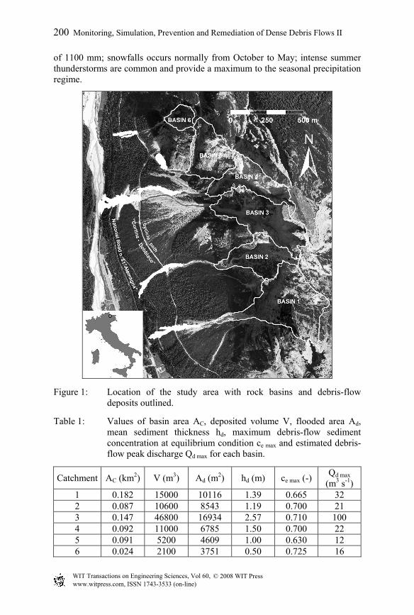
of 1100 mm; snowfalls occurs normally from October to May; intense summer thunderstorms are common and provide a maximum to the seasonal precipitation regime.

Figure 1: Location of the study area with rock basins and debris-flow deposits outlined.

Table 1: Values of basin area AC, deposited volume V, flooded area Ad, mean sediment thickness hd, maximum debris-flow sediment concentration at equilibrium condition ce max and estimated debris-flow peak discharge Qd max for each basin.

Catchment AC (km2) V (m3) Ad (m2) hd (m) ce max (-) Qd max

(m3 s-1) 1 0.182 15000 10116 1.39 0.665 32 2 0.087 10600 8543 1.19 0.700 21 3 0.147 46800 16934 2.57 0.710 100 4 0.092 11000 6785 1.50 0.700 22 5 0.091 5200 4609 1.00 0.630 12 6 0.024 2100 3751 0.50 0.725 16



Immediately after the 2006 event, field surveys were carried out in the study area. These surveys made it possible to measure several features of debris-flow deposits: mean and maximum depth, depth and slope of the deposition lobes and cross sections on the deposits. Moreover, cross-sections were measured along the main channel and a detailed description of debris-flow initiation areas were carried out. The boundaries of the debris-flow deposits were mapped using a handy GPS. The other geometric characteristics were measured using a laser distance meter and a tape. The LiDAR and photographic data was acquired from a helicopter using an ALTM 3100 OPTECH and Rollei H20 digital camera flying at an average altitude of 1000 m above ground level during snow free conditions in October 2006. The flying speed was 80 knots, the scan angle 20 degrees and the scan rate 71 KHz. The survey design point density was specified to be greater than 5 points per m2. LiDAR point measurements were filtered into returns from vegetation and bare ground using the TerrascanTM software classification routines and algorithms. The debris flows of July 5th, 2006 were triggered by an intense thunderstorm and hailstorm lasting from 6 p.m. to 7 p.m. The highest values of rainfall intensity during the event were 12.5 mm/5’ and 64 mm/h. These values were measured at a meteorological station located approximately 1 km from the study area. The debris flows initiated at the outlet of the rock basins, through the mobilization of loose debris into the flow with progressive entraining of debris from channel bank erosion and bed scour. The main channel stopped (at an altitude between 1441 m and 1553 m a.s.l.) where the slope angle decreases and consequently the depositional zone begins. The deposited volume was assessed by subtracting the 5 meter grid DEM of the post-event ground surface elevation (LiDAR data) with the pre-event DEM, derived from a topographic map on the scale of 1:5000. Water runoff from the rock basin was simulated by means of a hydrological model, which uses the CN method of the Soil Conservation Service (Chow et al [5]) to estimate the rainfall excess and a unit hydrograph to compute the flood hydrograph. On the basis of geological setting and land use of the basin upstream of the triggering point, we obtained an average value of CN = 84. The amount of the initial abstraction was set to the 10% of potential maximum retention to assess the excess rainfall. The concentration time was evaluated as the ratio between the main channel length and the flow velocity along the slopes (assumed to be equal to 2 m/s). The flood hydrograph was computed with a unit hydrograph (Chow et al [5]) extracted from a hypsographic curve by assuming the equivalence between the contour lines and the lines with the same concentration time. After the computation of six flood hydrographs, the following relation was adopted to infer debris-flow discharge from the water flood discharge (Takahashi [6]):

*1

cc

QQe

wd

−= (4)



where Qd is the debris flow discharge associated to the liquid discharge Qw; c* and ce are the “in situ” volumetric concentration of bed sediments before the flood and the debris-flow sediment concentration at equilibrium conditions respectively. Eqn. (4) refers to steady uniform conditions of a debris flow generated by a sudden release of Qw from the upstream end of an erodible and saturated grain bed. The assumption in eqn. (4) of a constant ratio ce/c* for the entire duration of the flood would be too severe a hypothesis in relation to the type of debris flow surges observed in the streams of the Dolomites (D’Agostino and Marchi [7]). Therefore the debris flow graph was plotted assuming a linear variation of ce/c* from a minimum value (ce min = 0.2) to a maximum (ce max) for each basin according to eqn. (4). The concentration ce max was calibrated to match the deposited debris-flow volumes with the reconstructed ones. Table 1 reports, for each catchment, the basin area AC, the deposited volume V, the flooded area Ad, the mean thickness hd of the debris-flow deposits (hd =V/Ad), the maximum debris-flow sediment concentration at equilibrium conditions ce max and the estimated debris-flow peak discharge Qd max.

4 Models application

Model calibration was carried out by comparing observed and computed characteristics of the deposits in terms of mean depth, flooded area, overall volume and shape of their boundaries. The calibration involved different input parameters for FLO-2D and RAMMS, because they follow different approaches and rheological laws. The computational domain in FLO-2D was assumed wholly as floodplain in order to achieve an unbiased comparison with RAMMS.

4.1 Input parameters

The adopted cell size was always 5 m in FLO-2D (vers.2006). To reproduce the terrain roughness, the following n values were assigned on the basis of land use (fig.1) in the depositional zone: n = 0.08 m-1/3s for debris areas, n = 0.14 m-1/3s for shrubs and n = 0.33 m-1/3s for forest. FLO-2D calibration was focused on the rheological parameters of viscosity and critical shear stress proposed by O’Brien [8]. Since the Fiames debris flows stopped at high slopes, always greater than 16°, the preliminary best simulations were carried out using the rheological scheme named “Aspen Pit 1” (O’Brien and Julien [4]) and setting K=24 in eqn. (2) (larger K values do not improve the quality of the results). In all cases this rheology reproduced deposits with an elongated shape and consequently overestimated runout distances. During the back analysis it has been noted that surface detention has a strong influence on the results and it can be used as a surrogate of the rheology. When the surface detention value increases the computed deposits assume a lower extent very quickly. As reported in table 2, the calibrated values of surface detention ranges between 0.10 m and 0.50 m. RAMMS model (beta vers.2007) calibration was related to the parameters which describe the debris-flow resistance. The dry friction factor (µ) was calculated as the surface slope of each debris-flow deposits along the terminal



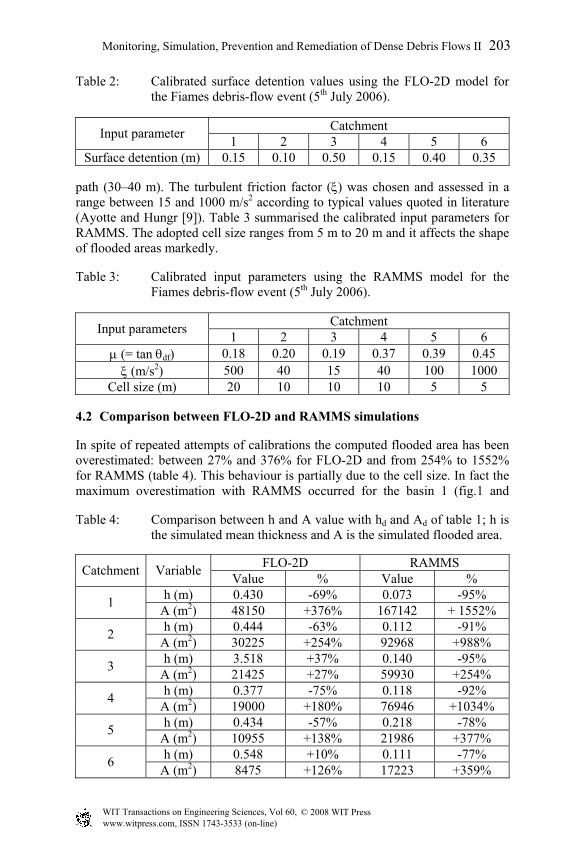
Table 2: Calibrated surface detention values using the FLO-2D model for the Fiames debris-flow event (5th July 2006).

Catchment Input parameter 1 2 3 4 5 6 Surface detention (m) 0.15 0.10 0.50 0.15 0.40 0.35

path (30–40 m). The turbulent friction factor (ξ) was chosen and assessed in a range between 15 and 1000 m/s2 according to typical values quoted in literature (Ayotte and Hungr [9]). Table 3 summarised the calibrated input parameters for RAMMS. The adopted cell size ranges from 5 m to 20 m and it affects the shape of flooded areas markedly.

Table 3: Calibrated input parameters using the RAMMS model for the Fiames debris-flow event (5th July 2006).

Catchment Input parameters 1 2 3 4 5 6 µ (= tan θdf) 0.18 0.20 0.19 0.37 0.39 0.45 ξ (m/s2) 500 40 15 40 100 1000

Cell size (m) 20 10 10 10 5 5

4.2 Comparison between FLO-2D and RAMMS simulations

In spite of repeated attempts of calibrations the computed flooded area has been overestimated: between 27% and 376% for FLO-2D and from 254% to 1552% for RAMMS (table 4). This behaviour is partially due to the cell size. In fact the maximum overestimation with RAMMS occurred for the basin 1 (fig.1 and

Table 4: Comparison between h and A value with hd and Ad of table 1; h is the simulated mean thickness and A is the simulated flooded area.

FLO-2D RAMMS Catchment Variable Value % Value % h (m) 0.430 -69% 0.073 -95% 1 A (m2) 48150 +376% 167142 + 1552% h (m) 0.444 -63% 0.112 -91% 2 A (m2) 30225 +254% 92968 +988% h (m) 3.518 +37% 0.140 -95% 3 A (m2) 21425 +27% 59930 +254% h (m) 0.377 -75% 0.118 -92% 4 A (m2) 19000 +180% 76946 +1034% h (m) 0.434 -57% 0.218 -78% 5 A (m2) 10955 +138% 21986 +377% h (m) 0.548 +10% 0.111 -77% 6 A (m2) 8475 +126% 17223 +359%



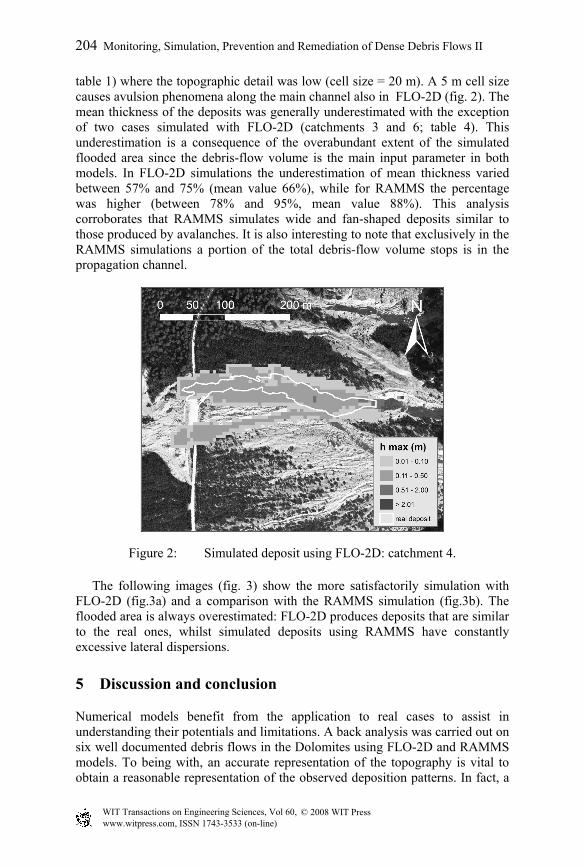
table 1) where the topographic detail was low (cell size = 20 m). A 5 m cell size causes avulsion phenomena along the main channel also in FLO-2D (fig. 2). The mean thickness of the deposits was generally underestimated with the exception of two cases simulated with FLO-2D (catchments 3 and 6; table 4). This underestimation is a consequence of the overabundant extent of the simulated flooded area since the debris-flow volume is the main input parameter in both models. In FLO-2D simulations the underestimation of mean thickness varied between 57% and 75% (mean value 66%), while for RAMMS the percentage was higher (between 78% and 95%, mean value 88%). This analysis corroborates that RAMMS simulates wide and fan-shaped deposits similar to those produced by avalanches. It is also interesting to note that exclusively in the RAMMS simulations a portion of the total debris-flow volume stops is in the propagation channel.

Figure 2: Simulated deposit using FLO-2D: catchment 4.

The following images (fig. 3) show the more satisfactorily simulation with FLO-2D (fig.3a) and a comparison with the RAMMS simulation (fig.3b). The flooded area is always overestimated: FLO-2D produces deposits that are similar to the real ones, whilst simulated deposits using RAMMS have constantly excessive lateral dispersions.

5 Discussion and conclusion

Numerical models benefit from the application to real cases to assist in understanding their potentials and limitations. A back analysis was carried out on six well documented debris flows in the Dolomites using FLO-2D and RAMMS models. To being with, an accurate representation of the topography is vital to obtain a reasonable representation of the observed deposition patterns. In fact, a



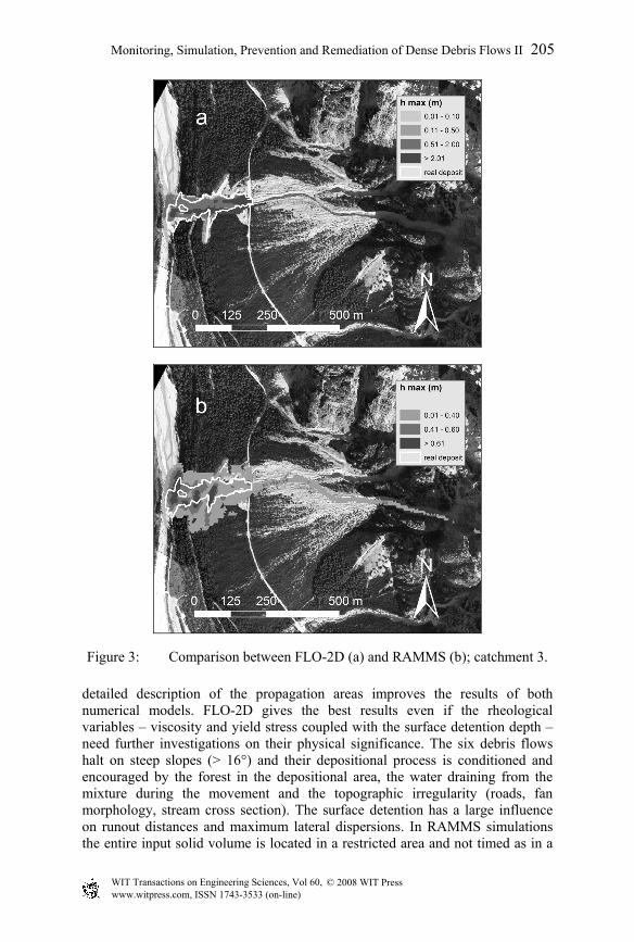
Figure 3: Comparison between FLO-2D (a) and RAMMS (b); catchment 3.

detailed description of the propagation areas improves the results of both numerical models. FLO-2D gives the best results even if the rheological variables – viscosity and yield stress coupled with the surface detention depth –need further investigations on their physical significance. The six debris flows halt on steep slopes (> 16°) and their depositional process is conditioned and encouraged by the forest in the depositional area, the water draining from the mixture during the movement and the topographic irregularity (roads, fan morphology, stream cross section). The surface detention has a large influence on runout distances and maximum lateral dispersions. In RAMMS simulations the entire input solid volume is located in a restricted area and not timed as in a



FLO-2D input hydrograph. Therefore the released debris flow suddenly reaches a channel that is insufficient to contain the entire discharge. As a consequence avulsion phenomena occur along the channel and they generate a larger lateral spreading than that observed in the field.

References

[1] O’Brien, J.S., Julien, P.Y. & Fullerton, W.T., Two-dimensional water flood and mudflow simulation. Journal of Hydraulic Engineering, 119(2), pp. 244–261, 1993.

[2] Voellmy, A., Ueber die Zerstoeerunskraft von Lawinen Schweizerische Bauzeitung. English version “On the destructive force of avalanches” translated by Tate R.E. (1964), ed. US Department of Agriculture Forest Service, 1955.

[3] Salm, B., Butkard, A. & Gubler, H., Berechnung von Fliesslawinen, eine Anleitung für Praktiker mit Beispielen. Mitteilung 47, Eigdenossichen Institut für Schnee und Lawinenforschung SLF Davos, 1990.

[4] O’Brien, J.S. & Julien, P.Y., Laboratory analysis of mudflows properties. Journal of Hydraulic Engineering, 114(8), pp. 877–887, 1988.

[5] Chow, V.T., Maidment, D.R. & Mays, L.W., Applied hydrology, McGraw-Hill: New York, pp. 201–236, 1988.

[6] Takahashi, T., Mechanical characteristics of debris flow. Journal of Hydraulic Division, 104, pp. 1153–1169, 1978.

[7] D’Agostino, V. & Marchi, L., Validation of semi-empirical relationships for the definition of debris-flow behaviour in granular materials. Proc. of the 3rd Int. Conf. on Debris Flows Hazard Mitigation: Mechanics, Prediction and Assessment, eds. D. Rickenmann & C.L. Chen, Millpress: Rotterdam, pp. 1097–1106, 2003.

[8] O’Brien, J.S., Physical processes, rheology and modelling of mudflows. Doctoral dissertation, Colorado State University, Fort Collins, Colorado, 1986.

[9] Ayotte, D. & Hungr, L., Calibration of a runout prediction model for debris flow and avalanches, Proc. of the 2nd Int. Conf. on Debris Flows Hazard Mitigation: Mechanics, Prediction and Assessment, eds. G.F. Wieczorek & N.D. Naeser, Balkema: Rotterdam, pp. 505–514, 2000.



Documents

Comparison between FLO-2D and RAMMS in debris-flow ... · Comparison between FLO-2D and RAMMS in debris-flow modelling: a case study in the Dolomites M. Cesca & V. D’Agostino Department