I

COMPARISON BETWEEN THREE

DIFFERENT CFD SOFTWARE AND

NUMERICAL SIMULATION OF AN

AMBULANCE HALL

Ning Li

Master of Science Thesis

KTH School of Industrial Engineering and Management

Energy Technology EGI-2015-017MSC

Division of Energy Technology

SE-100 44 STOCKHOLM

-II-

Master of Science Thesis EGI 2015: 017MSC

Comparison between three different CFD

software and numerical simulation of an

ambulance hall

Ning Li

Approved

2015-03-05

Examiner

Joachim Claesson

Supervisor

Joachim Claesson

Commissioner

SWECO Systems AB

Contact person

David Burman

Liu Ting

Abstract

Ambulance hall is a significant station during emergency treatment. Patients need to be transferred from

ambulance cars to the hospital’s building in the hall. Eligible performance of ventilation system to supply

satisfied thermal comfort and healthy indoor air quality is very important. Computational fluid dynamic

(CFD) simulation as a broadly applied technology for predicting fluid flow distribution has been

implemented in this project.

There has two objectives for the project. The first objective is to make comparison between the three

CFD software which consists of ANSYS Fluent, Star-CCM+ and IESVE Mcroflo according to CFD

modeling of the baseline model. And the second objective is to build CFD modeling for cases with

difference boundary conditions to verify the designed ventilation system performance of the ambulance

hall.

In terms of simulation results from the three baseline models, ANSYS Fluent is conclusively

recommended for CFD modeling of complicated indoor fluid environment compared with Star-CCM+

and IESVE Microflo. Regarding to the second objective, simulation results of case 2 and case 3 have

shown the designed ventilation system for the ambulance hall satisfied thermal comfort level which

regulated by ASHRAE standard with closed gates. Nevertheless, threshold limit value of the contaminants

concentration which regulated by ASHRAE IAQ Standard cannot be achieved. From simulation results of

case 4.1 to 4.3 shown that the designed ventilation system cannot satisfy indoor thermal comfort level

when the gates of the ambulance hall opened in winter. In conclusion, measures for decreasing

contaminants concentration and increasing indoor air temperature demanded to be considered in further

design.

-III-

Table of Contents

Abstract .......................................................................................................................................................................... II

Acknowledgements ...................................................................................................................................................... V

List of Figures ............................................................................................................................................................. VI

List of Tables ............................................................................................................................................................ VIII

Nomenclature.............................................................................................................................................................. IX

1 Introduction .......................................................................................................................................................... 1

1.1 Background .................................................................................................................................................. 1

1.2 Objectives ..................................................................................................................................................... 2

1.3 Method .......................................................................................................................................................... 3

2 Numerical principle of simulation ..................................................................................................................... 4

2.1 Governing Equations ................................................................................................................................. 4

2.1.1 Conservation laws of fluid flow. ...................................................................................................... 4

2.1.2 Thermal equations of wall boundary condition. ........................................................................... 4

2.2 Turbulence modeling .................................................................................................................................. 5

2.2.1 Different choice of k-ε Model ......................................................................................................... 5

2.2.2 Near – Wall functions ....................................................................................................................... 7

2.3 Meshing ........................................................................................................................................................ 8

2.3.1 Shapes of Cell ..................................................................................................................................... 8

2.3.2 Classification of Grids ....................................................................................................................... 8

2.3.3 Mesh Quality ....................................................................................................................................... 9

2.4 Solver...........................................................................................................................................................10

2.4.1 Finite Volume Method ....................................................................................................................10

2.4.2 Upwind scheme ................................................................................................................................11

2.4.3 SIMPLE Scheme ..............................................................................................................................11

3 Baseline model and Comparison between Software ....................................................................................13

3.1 Data of ventilation system for baseline model. ....................................................................................13

3.1.1 Design Concept ................................................................................................................................13

3.1.2 Parameter of supply air diffuser ....................................................................................................13

3.1.3 Parameter of Exhaust Grilles .........................................................................................................13

3.2 Geometry ....................................................................................................................................................14

3.3 Meshing ......................................................................................................................................................15

3.3.1 Meshing Independency ...................................................................................................................15

3.3.2 Meshing Method ..............................................................................................................................17

3.4 Numerical Setup ........................................................................................................................................19

3.4.1 Selection of simulation models ......................................................................................................19

3.4.2 Boundary conditions .......................................................................................................................19

-IV-

3.4.3 Solution Control ...............................................................................................................................21

3.5 Simulation results ......................................................................................................................................23

3.5.1 Assessment of thermal comfort in an arbitrary point. ...............................................................23

3.5.2 Velocity Distribution .......................................................................................................................24

3.5.3 Temperature Distribution ...............................................................................................................28

4 Ventilation Performance in Different Situations ..........................................................................................33

4.1 Geometry ....................................................................................................................................................33

4.1.1 Case 2: Improved ventilation system. ...........................................................................................33

4.1.2 Case 3: Polluted emission from tailpipes of the ambulance cars. ............................................34

4.1.3 Case 4.1-4.3: With opened gates and installed air curtains. .......................................................34

4.2 Meshing ......................................................................................................................................................36

4.3 Boundary Conditions Setup ....................................................................................................................36

4.3.1 Case 2: Improved ventilation system. ...........................................................................................36

4.3.2 Case 3: Polluted emission from tailpipes of the ambulance cars. ............................................36

4.3.3 Case 4.1-4.3: With opened gates and installed air curtains. .......................................................37

4.4 Simulation Results and Analysis. ............................................................................................................38

4.4.1 Case 2: Improved ventilation system. ...........................................................................................38

4.4.2 Case 3: Polluted emission from tailpipes of the ambulance cars. ............................................40

4.4.3 Case 4.1-4.3: With opened gates and installed air curtains. .......................................................43

4.5 Optimized approaches for improving thermal comfort. ....................................................................48

4.5.1 One more supply air diffuser on the specified wall. ...................................................................48

4.5.2 Exhaust extraction system. .............................................................................................................49

4.5.3 Supplement of heat in winter. ........................................................................................................49

5 Conclusion and future improvement ..............................................................................................................51

6 Bibliography ........................................................................................................................................................52

Appendix A: Data sheet/Dimension of Jet Nozzle Diffuser ..............................................................................54

Appendix B: Data and Dimension of Exhaust Grilles ..........................................................................................55

Appendix C: Data and Type of Air curtain. ............................................................................................................56

Appendix D: CO Level vs. Condition&Health Effects. .......................................................................................57

-V-

Acknowledgements

Foremost I would like to express my fully gratitude to Will Sibia from SWECO systems AB, Stockholm

Sweden for giving me the opportunity to do my master thesis within such interesting and cutting edge

field by a practical project.

Specially, I would like to extend my deepest thanks to Liu Ting, who is my thesis supervisor from

SWECO in the field of CFD simulation. Encouragements, professional and theoretical supports from her

were very beneficial and helpful for me to complete the project.

Sincerely, I would also very thankful to David Berman, who is my thesis supervisor from SWECO in the

field of energy technology and ventilation systems design. Professional advices and positive feedbacks

from him supervised me done the project in the right way.

Moreover, I would like to express my grate gratitude to my supervisor, Associate Professor Joachim

Claesson, at the Royal Institute of Technology (KTH) for your fully helpful supports, responsible

feedback and all the fantastic knowledge were taught from you during the graduate study.

Finally, I am deep appreciate to my parents, my friends for their love and supports.

-VI-

List of Figures

Figure 1, 3D layout of SÖS ambulance hall. ..................................................................................................................... 1

Figure 2, Project Outline .................................................................................................................................................... 2

Figure 3, Velocity distribution near a wall (Versteeg & Malalasekera, 2007) ............................................................... 7

Figure 4, Typical 2D control volume (Versteeg & Malalasekera, 2007). ....................................................................... 8

Figure 5, Block-structured mesh (left) and Unstructured mesh (right) of aerofoil (Versteeg & Malalasekera, 2007) ........ 8

Figure 6, Comparison between coarse, medium and fine hybrid grid. .................................................................................... 9

Figure 7, Misalignment of midpoints for skewed grid. ......................................................................................................... 9

Figure 8, Conservation of general flow variable within finite volume method (Versteeg & Malalasekera, 2007).............10

Figure 9, Evaluation of face value according to Upwind Scheme (Cho, et al., 2010). ......................................................11

Figure 10, Calculation process of SIMPLE Scheme (Versteeg & Malalasekera, 2007)...............................................12

Figure 11, Air motion of Group A outlets (ASHRAE, 1997). ......................................................................................13

Figure 12, Geometry of the ambulance hall .......................................................................................................................14

Figure 13， Face sizing for air inlet (Left: Element size is 0.05m; Right: Element size is 0.03m) ..................................15

Figure 14, Face sizing for air outlet (Left: Element size is 0.1m; Right: Element size is 0.05m) ......................................16

Figure 15, Velocity distribution for the two different meshing cases. ...................................................................................16

Figure 16, Generated mesh of the ambulance hall in IESVE Microflo. ...........................................................................17

Figure 17, Generated mesh of the ambulance hall in ANSYS mesh. ................................................................................17

Figure 18, Section plane of (a) Air Inlet; (b) Air Outlet; (c) Exterior Wall; (d) Internal space ........................................18

Figure 19, Mesh metrics control of ANSYS mesh (Left: Skewness; Right: Aspect Ratio) ................................................18

Figure 20, Cell Monitor of point in Case 1.3. ..................................................................................................................23

Figure 21, PPD as a function of PMV (ISO, 1994). ....................................................................................................23

Figure 22, Thermal comfort zone display in Psychronmetric chart. ....................................................................................24

Figure 23, Vector of velocity distribution (h=3m) of case 1.1. ..........................................................................................25

Figure 24, Velocity Magnitude (h=3m) of case 1.1. (Left: 0 to 5.02m/s, Right: 0 to 1 m/s) ..........................................25

Figure 25, Vector of Velocity distribution (h=1m) of case 1.1. ........................................................................................25

Figure 26, Zoomed-in views of velocity distribution at plant (h=1m).s ..............................................................................26

Figure 27, Vector of velocity distribution (h=3m) of case 1.2. ..........................................................................................26

Figure 28, Vector of velocity distribution (h=1m) of case 1.2. ..........................................................................................27

Figure 29, Vector and contour of velocity distribution (h=3m and h=1m) of case 1.3. ......................................................27

Figure 30, Local mean age of air (h=1m) of case 1.3. ......................................................................................................28

Figure 31, Temperature distribution (h=1m, local temperature). .......................................................................................29

Figure 32, Temperature distribution (h=1m, specified temperature). .................................................................................29

Figure 33, Temperature distribution (h=1m, global temperature) with isosurface. ..............................................................30

Figure 34, Temperature distribution (Left: x=3.6m, 11m and 18.3m; Right: y=10.3m, 15.5m and 21m). ...................30

Figure 35, Temperature distribution on envelop of ambulance hall.....................................................................................30

Figure 36, Temperature distribution of case 1.2. ...............................................................................................................31

Figure 37, Temperature distribution of case 1.3. ...............................................................................................................32

Figure 38, Geometry of case 2 with 4 exhaust grilles. .......................................................................................................33

Figure 39, Geometry of case 3 with tailpipe emission (Left: whole room; Right: zoomed-in to the tailpipe) .........................34

Figure 40, Configuration of air curtain which installed in case 4.1-4.3. ............................................................................34

Figure 41, Geometry of case 4.1 - 4.3. .............................................................................................................................35

Figure 42, Zoomed-in views of geometry for case 4.1-4.3. ..................................................................................................35

Figure 43, Meshing of case 4.1-4.3 (Left: Global: Right: Section cut view). ......................................................................36

Figure 44, Velocity distribution at h=3m over the ground (Local Velocity). .....................................................................38

Figure 45, Velocity distribution at h=1m (Local Velocity). .............................................................................................38

Figure 46, Zoomed-in views to figure 45. ..........................................................................................................................39

Figure 47, Temperature distribution of case 2 at h=1m (Left: local temperature, Right: Specified temperature). ................39

Figure 48, Temperature distribution of case 2 (Left: h=0.1m, isosurface=18C; Right: Room Envelope). .........................40

Figure 49, Velocity distribution of case 3 (Left: h=3m; Right: h=0.4m) .........................................................................40

-VII-

Figure 50, Velocity distribution of case 3 (h=1m). ...........................................................................................................41

Figure 51, Temperature distribution of case 3 h=0.4m (Left: Local temperature; Right: specified temperature) .................41

Figure 52, Temperature distribution of case 3 at h=1m (Specified Temperature). ..............................................................42

Figure 53, CO concentration distribution of case 3 (h=1.5m). ..........................................................................................42

Figure 54, CO2 concentration distribution of case 3 (h=1.5m). .......................................................................................43

Figure 55, Velocity distribution of case 4.1 (h=1m) .........................................................................................................44

Figure 56, Specified velocity of case 4.1 at h=1m (Left: Velocity 0m/s - 0.2m/s; Right: Velocity 0m/s - 1m/s). ...........44

Figure 57, Velocity distribution of case 4.1 around the opened gates. ................................................................................45

Figure 58, Temperature distribution of case 4.1 (Left=3m; Right=1m). ..........................................................................45

Figure 59, Temperature distribution of case 4.1 (Transection view at gate). .......................................................................46

Figure 60, Pressure distribution at h=1m of case 4.2(Left) and case 4.3 (Right). .............................................................46

Figure 61, Pressure change along the line of case 4.2(red line) and case 4.3 (blue line). ......................................................46

Figure 62, Velocity distribution at h=1m of case 4.2(Left) and case 4.3 (Right). .............................................................47

Figure 63，Zoomed-in Velocity distribution at h=1m of case 4.2(Left) and case 4.3 (Right). .........................................47

Figure 64, Temperature distribution at h=1m of case 4.2(Left) and case 4.3 (Right). ......................................................48

Figure 65, Install position of the additional supply air diffuser. .........................................................................................48

Figure 66, Conventional exhaust extraction system (Left) and "in ground" exhaust extraction system (Right). ..................49

Figure 67, Working principle of "in ground" exhaust extraction system (Nenerman, 2014). .........................................49

-VIII-

List of Tables

Table 1, Cade name of different cases.................................................................................................................................. 2

Table 2, Skewness range and cell quality (Fluent, 2006). ...............................................................................................10

Table 3, Input dimensions of geometry of the ambulance hall. ............................................................................................14

Table 4, Performance of 3D modeling for different tools. ...................................................................................................15

Table 5, Comparison of Mass flow rate and Total heat transfer rate between the two meshing cases .........16

Table 6, Statistics of mesh which generated from ANSYS mesh and IES VE – CFD Grid. .........................................18

Table 7, Performance of meshing for the three software. .....................................................................................................18

Table 8, Boundary Conditions set up in ANSYS Fluent and Star - CCM+. .................................................................20

Table 9, Solution control for the three software. .................................................................................................................22

Table 10, Performance of numerical setup for the three software. ........................................................................................22

Table 11, Thermal sensation scale for PMV Method. ......................................................................................................23

Table 12, Simulation results of the three software. ............................................................................................................32

Table 13, Different between the two types of exhaust grilles in two cases. ...........................................................................33

Table 14, Additional parameters of geometry for case 4.1 to 4.3. ......................................................................................34

Table 15, Input parameters for boundary conditions of tailpipes. .......................................................................................37

Table 16, Air curtain boundary conditions of case 4.1-4.3. ..............................................................................................37

-IX-

Nomenclature

Symbols

A area

Cp specific heat

Ci contaminant concentration

Cu k-epsilon model constant

g gravitational constant

hext external heat transfer coefficient

hf heat transfer coefficient of the fluid side

I tensor of unit

k thermal conductivity

P pressure

Q heat transfer rate

Sm source of mass

T Temperature

t time

u velocity

V volumetric flow rate

y+ dimensionless wall distance

dissipation rate of k

ext emissivity

k turbulence kinetic energy

Stefan-Boltzmann constant

,T l laminar Prandtl number

,T t turbulent Prandtl number

Φ flow variable

under-relaxation factor

near-wall temperature equation constant

ρ density

Ωij rate-of-rotation tensor

i local mean age of air

stress tensor

viscosity of molecular

Abbreviations

CFD Computational Fluid Dynamic

FVM Finite Volume Method

LMA Local Mean Age

PMV Predicted Mean Vote

PPD Percentage of Dissatisfied

RNG Re-Normalization Group

SIMPLE Semi-Implicit Method for Pressure-Linked Equations

1

1 Introduction

1.1 Background

Numerical visualization is a platform provides a simpler way to analysis of large, complex and muti-

dimensional information. Computational fluid dynamic, also called CFD, has combined fluid mechanic

with this platform to simulate both compressible and incompressible fluid flow behavior. Distribution of

temperature, velocity, pressure, contaminant concentration and other fluid properties can be calculated

and displayed from results of CFD simulation (Stamou, et al., 2007). Output results help engineers to

improve and consummate their design quickly and effectively.

In this project, three different CFD commercial software have been employed by the author to evaluate

indoor thermal comfort of an ambulance hall which is belong to SÖS hospital renovation project from

SWECO, in Stockholm, Sweden. As defined by international standard ISO 7730, thermal comfort as

“condition of mind which expresses satisfaction of thermal environment” has explained that comfort level

need to be determined by subject method (ISO, 1994). According to the criteria ISO 7730, metabolic rate

(MET) and thermal insulation of clothing index (CLO) will be introduced for obtain thermal comfort

indexes which are predicted mean vote (PMV) and predicted percentage of dissatisfied (PPD) (ISO, 1994).

The three different CFD commercial software consist of ANSYS - Fluent, IES VE – Microflo and Star –

CCM+. Internal analyses of the ambulance hall were established by the three tools for baseline case.

Thereafter, three additional modeling cases which include improvement of ventilation system, hall with

tailpipe emissions and opened gates with natural ventilation were implemented by ANSYS – Fluent

independently.

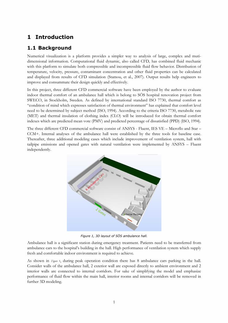
Figure 1, 3D layout of SÖS ambulance hall.

Ambulance hall is a significant station during emergency treatment. Patients need to be transferred from

ambulance cars to the hospital’s building in the hall. High performance of ventilation system which supply

fresh and comfortable indoor environment is required to achieve.

As shown in Figure 1, during peak operation condition there has 8 ambulance cars parking in the hall.

Consider walls of the ambulance hall, 2 exterior wall are exposed directly to ambient environment and 2

interior walls are connected to internal corridors. For sake of simplifying the model and emphasize

performance of fluid flow within the main hall, interior rooms and internal corridors will be removed in

further 3D modeling.

-2-

1.2 Objectives

Two main objectives of the project had been set up.

The first objective is to build CFD modeling in three different numerical simulation software which have

been specified as ANSYS-Fluent, IES VE - Microflo and Star-CCM+. Thereafter, made comparison of

performance among these three software.

The second objective is to optimize ventilation system according to output results from baseline model,

simulate the optimized model while involving exhaust emission from the ambulance cars or natural

ventilation with opening gates.

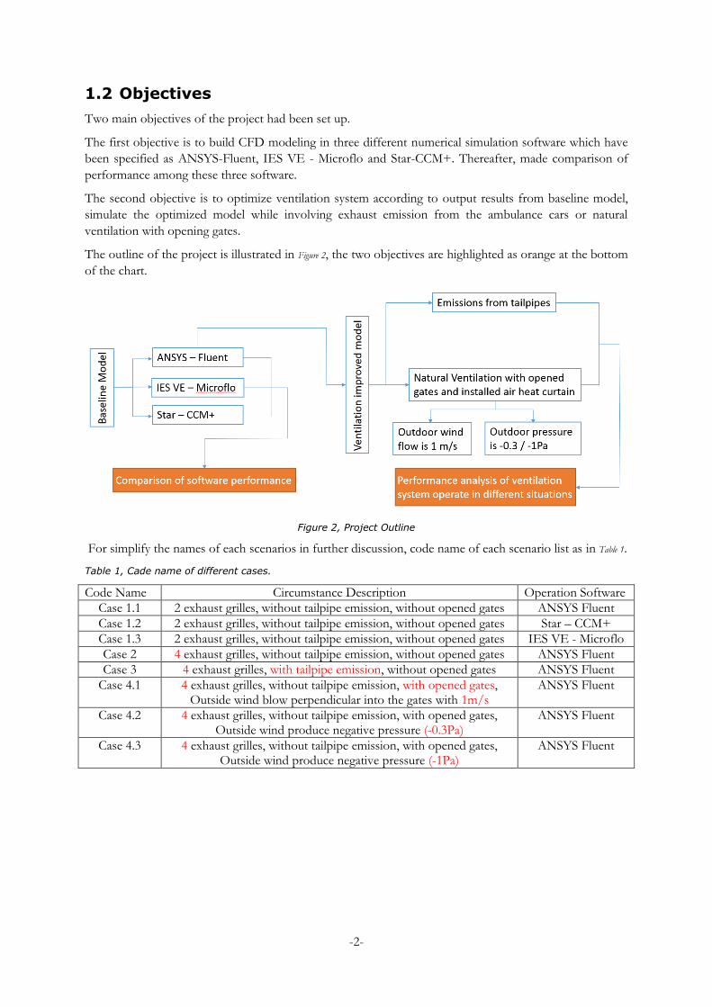
The outline of the project is illustrated in Figure 2, the two objectives are highlighted as orange at the bottom

of the chart.

Figure 2, Project Outline

For simplify the names of each scenarios in further discussion, code name of each scenario list as in Table 1.

Table 1, Cade name of different cases.

Code Name Circumstance Description Operation Software

Case 1.1 2 exhaust grilles, without tailpipe emission, without opened gates ANSYS Fluent

Case 1.2 2 exhaust grilles, without tailpipe emission, without opened gates Star – CCM+

Case 1.3 2 exhaust grilles, without tailpipe emission, without opened gates IES VE - Microflo

Case 2 4 exhaust grilles, without tailpipe emission, without opened gates ANSYS Fluent

Case 3 4 exhaust grilles, with tailpipe emission, without opened gates ANSYS Fluent

Case 4.1 4 exhaust grilles, without tailpipe emission, with opened gates, Outside wind blow perpendicular into the gates with 1m/s

ANSYS Fluent

Case 4.2 4 exhaust grilles, without tailpipe emission, with opened gates, Outside wind produce negative pressure (-0.3Pa)

ANSYS Fluent

Case 4.3 4 exhaust grilles, without tailpipe emission, with opened gates, Outside wind produce negative pressure (-1Pa)

ANSYS Fluent

-3-

1.3 Method

Numerical simulation based on computational fluid dynamic (CFD) has become broadly used for

predicting fluid behavior within the objective domain. With foreseeable fluid distribution, undesirable

fluids have the possibility to be decreased or avoided through improvement of the design.

All the simulated cases implemented in this project were built in terms of computational fluid dynamic.

However, turbulence model, boundary conditions, mesh method, simulation scheme and etc. regarding to

modelling setup have to be decided for each case.

In order to decide adaptable modeling schemes implemented during the setup, literature review from

relative scientific papers and corresponding international standards was applied in Chapter 2 and setup of

boundary conditions in Chapter 3 and 4. For comparison among the cases in different circumstances, case

studies with different boundary conditions will be analyzed and disused in Chapter 3 and Chapter 4.

Finally, improved approaches for optimizing the design of the cases will be analyzed briefly.

-4-

2 Numerical principle of simulation

Numerical method for calculating air flow behavior and heat transfer performance is a more beneficial

approach compared with corresponding experiments. Both spending of time and cost can be saved

significantly. Among with multi-fields application, numerical simulation of internal air pattern of building

is developed rapidly during recent years. Detailed information of air temperature, velocity components,

and pressure drop and turbulence intensity within the modeling domain can be generated simultaneously

by CFD software.

2.1 Governing Equations

2.1.1 Conservation laws of fluid flow.

The conservation laws of fluid flow defined by Versteeg and Malalasekera (Versteeg & Malalasekera, 2007)

applies on three fundamental variable quantities which are momentum, energy and mass of fluid particle.

On the base of Newton’s second law, the sum of the forces on a fluid particle is equaled to the rate of

change of momentum. According to first law of thermodynamics, energy changing rate on a fluid particle

is equal to the work done by the particle plus the rate of heat added to it. Meanwhile, mass of fluid is

conserved. Conservation equations which required for simulation are list as followed:

For conservation of mass (Eleni, et al., 2012):

( ) Smu

t

(1)

Where Sm is the source from dispersed second phase and to be added to the continuous phase.

For conservation of momentum (Fluent, 2006):

( ) ( ) ( )v vv P g F

t

(2)

Where is stress tensor and expressed as below (Fluent, 2006):

2

3

T

v v vI

(3)

In equation (3), is the viscosity of molecular, I is the tensor of unity.

For energy equation in three dimension, four terms are associated with energy changed in the fluid particle

(Versteeg & Malalasekera, 2007):

xy xy yyxx zx

E

zy yzxz zz

u v vu u

x y z x yDEdiv pu div kgradT S

Dt v ww w

z x y z

(4)

2.1.2 Thermal equations of wall boundary condition.

Five types of thermal condition which includes fixed heat flux, fixed temperature, convection, radiation

and mixed for wall boundary layer are provided by ANSYS Fluent. Considering to predict fluid flow

within the ambulance hall be more accurate, heat transfer through wall (and near wall) boundary by

conduction, convection and radiation are overall calculated.

-5-

Heat transfer rate through boundary of wall by conduction:

cond

dTQ kA

ds (5)

Where k is the average thermal conductivity of material of wall.

For walls which with external radiation boundary condition, heat transfer rate expresses as:

4 4

rad f w f rad ext wQ h T T q T T (6)

Where both ext (emissivity of external wall) and T

(temperature of external domain) are required to be

defined manually in ANSYS FLUENT and Star-CCM+.

For walls which with boundary condition of combined external convection and radiation, equation of heat

transfer rate shows as:

4 4

mixed f w f rad ext ext w ext wQ h T T q h T T T T (7)

Where exth is the external heat transfer coefficient that to be defined according to dry-bulb temperature of

outside environment.

For equation 6 and 7, wT is the surface temperature of the wall, fh is the heat transfer coefficient of the

fluid side, is Stefan-Boltzmann constant.

2.2 Turbulence modeling

The Navier – Stokes equations which arise from Newton’s second law is to describe viscous flow in

multiply application. A suitable model for viscous stresses component ij and pressure term are introduced

to the conservation equations. As formed by Versteeg and Malalasekera (Versteeg & Malalasekera, 2007),

the Navier – Stokes equations can be written for finite volume method (which will be discussed in section

2.5) in the most useful form as:

Mx

Du pdiv gradu S

Dt x

(8)

For three dimensional fluid flow, the equation 8 also identically applies on y and z direction with velocity

vectors v and w .

2.2.1 Different choice of k-ε Model

Supplemented with turbulence model based on Navier – Stokes equations which implemented in practical

CFD applications, the most appropriate viscous model for numerical simulation of high Reynold number

is k-epsilon (2eqn) viscous model (Calautit, et al., 2012). In ANSYS Fluent there has three transport

equations related to k-epsilon model, the standard k-epsilon model, RNG k model and the Realizable

k Model. As demonstrated by Tsan-Hsing and et al. (Shih, et al., 1994), realizable k Model

performs the best of all versions of k Model from several validations of flows with complex

secondary features and separated flows. In Star-CCM+, there has eight different transformation equations

for choice of k turbulence model. However, only standard k turbulence model provided by IES

VE Microflo. Therefore, both standard and realizable k model have been implemented during

numerical modeling in this project.

For standard k model, the turbulence kinetic energy k and its dissipation rate , can be calculated

from equations below (Fluent, 2006):

-6-

ti k b M k

i j k j

kk ku G G Y S

t x x x

(9)

And

2

1 3 2t

i k b

i j j

ku C G G G C St x x x k k

(10)

The term kG as shown in above equations is the production of turbulence energy due to mean velocity

gradients which defined as:

' ' j

k i j

i

uG u u

x

(11)

The term bG as shown represents production of turbulence energy due to buoyancy effect which defined

as:

t

b i

t i

TG g

Pr x

(12)

The viscosity of turbulence flow,t is calculated by combination of k and as follow:

2

t

kC

(13)

And for constants in the equations 9 and 10 are listing as (Markatos , 2004):

1C = 1.44, 2C =1.92, C =0.09,

k =1.0 and =1.3

For realizable k model, the turbulence kinetic energy k and its dissipation rate , can be calculated

from equations below (Shih, et al., 1994):

tj k b M k

j j k j

kk ku G G Y S

t x x x

(14)

And

2

1 2 1 3t

j b

j j j

u C S C C C G St x x x kk v

(15)

Where,

1 max 0.43, , , 25

ij ij

kC S S S S

(16)

Differ from standard k model, C is not constant any more, it need to be computed from:

*

0

1

S

CkU

A A

(17)

Where, *

ij ij ij ijU S S (18)

And

2ij ij ijk k ; ij ij ijk k ;0A =4.04, 6 cosSA

Where,

-7-

11cos 6

3W ,

3

ij jk ktS S SW

S ,

ij ijS S S , 1

2

j iij

i j

u uS

x x

(19)

And for constants in the equations 14 and 15 are listing as (Fluent, 2006):

1C = 1.44, 2C =1.9,

k =1.0 and =1.2

The generation of the turbulence kinetic energy is calculated in the same way for both standard and

realizable k model except for value of constants, with the same kG and

bG representation which

shows in equation 11 and 12.

2.2.2 Near – Wall functions

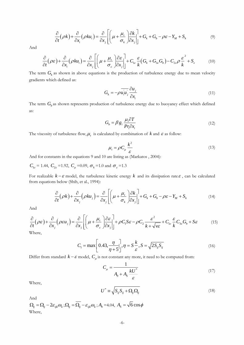
Gradient of velocity changed in near-wall region is usually strong for no-slip walls. As shown in Figure 3,

according to mathematical and experiments analysis, near-wall region can be separated into two layers

which are laminar flow (linear sublayer) and turbulence flow (Versteeg & Malalasekera, 2007). Regions are

subdivided by point P shown in Figure 3.

Figure 3, Velocity distribution near a wall (Versteeg & Malalasekera, 2007)

When value of yis larger than 11.63 (above point P), mean velocity of turbulence flow is considered to

be in log-law region and can be yielded as:

1lnU Ey

(20)

Where y+ shows as equation below:

*yuy

v

(21)

And temperature distribution for turbulence flow in near wall region is computed as (Launder & Spalding,

1973):

,

,

,

T l

T t

T t

T u P

(22)

Where in equation 20 and 21, is 0.4187, E is constant shear stress 9.793 for smooth walls, ,T l and

,T t are laminar and turbulent Prandtl number.

In order to obtain the most accurate velocity profile in near-wall region, not only computational equations but also intensive mesh with high equality are required to be applied during the simulation. Therefore, inflation layers which can help to improve mesh quality will be discussed later in following chapters.

-8-

2.3 Meshing

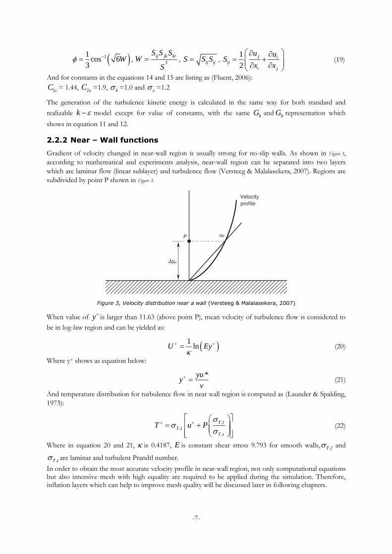
2.3.1 Shapes of Cell

Mesh quality during pre-processing is very significant for CFD simulation results. Grid of simulation

object is generated upon the completed geometry. Both polygonal and polyhedral mesh is practicably

applied. As some simple examples list by (Versteeg & Malalasekera, 2007) and shown in Figure 4, different

shapes of control volumes are used for surface meshing (2D). And in volume meshing (3D), triangular or

quadrilateral surface elements helps to bind the 3D control volume.

Figure 4, Typical 2D control volume (Versteeg & Malalasekera, 2007).

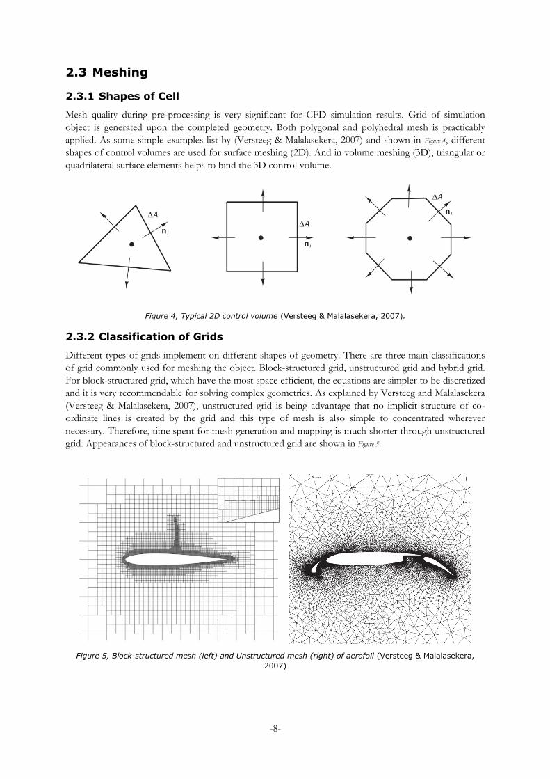
2.3.2 Classification of Grids

Different types of grids implement on different shapes of geometry. There are three main classifications

of grid commonly used for meshing the object. Block-structured grid, unstructured grid and hybrid grid.

For block-structured grid, which have the most space efficient, the equations are simpler to be discretized

and it is very recommendable for solving complex geometries. As explained by Versteeg and Malalasekera

(Versteeg & Malalasekera, 2007), unstructured grid is being advantage that no implicit structure of co-

ordinate lines is created by the grid and this type of mesh is also simple to concentrated wherever

necessary. Therefore, time spent for mesh generation and mapping is much shorter through unstructured

grid. Appearances of block-structured and unstructured grid are shown in Figure 5.

Figure 5, Block-structured mesh (left) and Unstructured mesh (right) of aerofoil (Versteeg & Malalasekera,

2007)

-9-

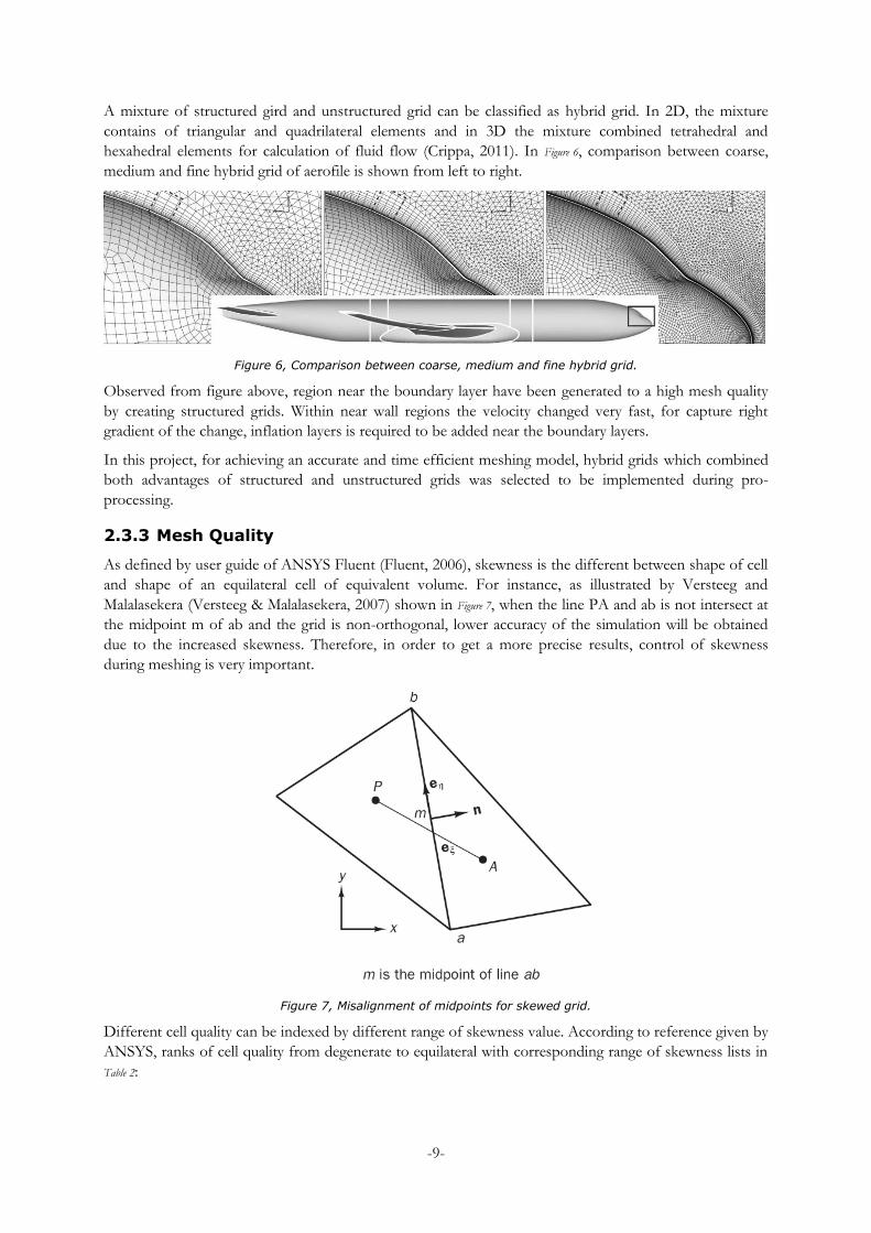
A mixture of structured gird and unstructured grid can be classified as hybrid grid. In 2D, the mixture

contains of triangular and quadrilateral elements and in 3D the mixture combined tetrahedral and

hexahedral elements for calculation of fluid flow (Crippa, 2011). In Figure 6, comparison between coarse,

medium and fine hybrid grid of aerofile is shown from left to right.

Figure 6, Comparison between coarse, medium and fine hybrid grid.

Observed from figure above, region near the boundary layer have been generated to a high mesh quality

by creating structured grids. Within near wall regions the velocity changed very fast, for capture right

gradient of the change, inflation layers is required to be added near the boundary layers.

In this project, for achieving an accurate and time efficient meshing model, hybrid grids which combined

both advantages of structured and unstructured grids was selected to be implemented during pro-

processing.

2.3.3 Mesh Quality

As defined by user guide of ANSYS Fluent (Fluent, 2006), skewness is the different between shape of cell

and shape of an equilateral cell of equivalent volume. For instance, as illustrated by Versteeg and

Malalasekera (Versteeg & Malalasekera, 2007) shown in Figure 7, when the line PA and ab is not intersect at

the midpoint m of ab and the grid is non-orthogonal, lower accuracy of the simulation will be obtained

due to the increased skewness. Therefore, in order to get a more precise results, control of skewness

during meshing is very important.

Figure 7, Misalignment of midpoints for skewed grid.

Different cell quality can be indexed by different range of skewness value. According to reference given by

ANSYS, ranks of cell quality from degenerate to equilateral with corresponding range of skewness lists in

Table 2:

-10-

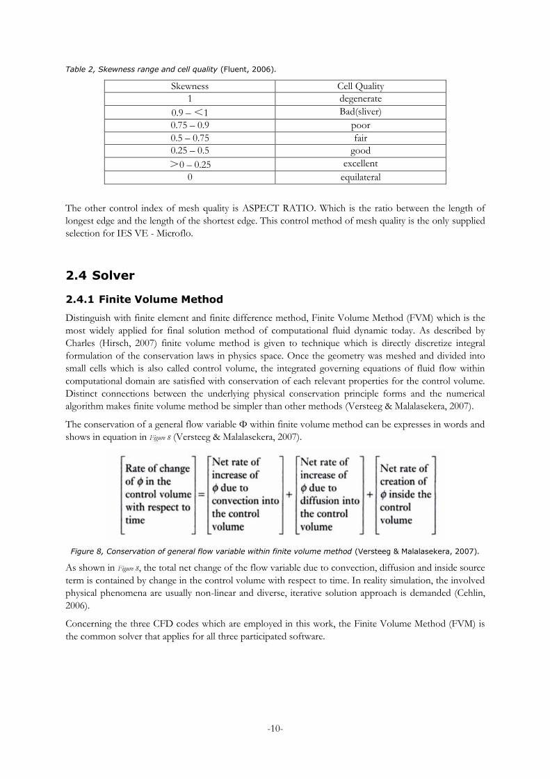
Table 2, Skewness range and cell quality (Fluent, 2006).

Skewness Cell Quality

1 degenerate

0.9 – ＜1 Bad(sliver)

0.75 – 0.9 poor

0.5 – 0.75 fair

0.25 – 0.5 good

＞0 – 0.25 excellent

0 equilateral

The other control index of mesh quality is ASPECT RATIO. Which is the ratio between the length of

longest edge and the length of the shortest edge. This control method of mesh quality is the only supplied

selection for IES VE - Microflo.

2.4 Solver

2.4.1 Finite Volume Method

Distinguish with finite element and finite difference method, Finite Volume Method (FVM) which is the

most widely applied for final solution method of computational fluid dynamic today. As described by

Charles (Hirsch, 2007) finite volume method is given to technique which is directly discretize integral

formulation of the conservation laws in physics space. Once the geometry was meshed and divided into

small cells which is also called control volume, the integrated governing equations of fluid flow within

computational domain are satisfied with conservation of each relevant properties for the control volume.

Distinct connections between the underlying physical conservation principle forms and the numerical

algorithm makes finite volume method be simpler than other methods (Versteeg & Malalasekera, 2007).

The conservation of a general flow variable Φ within finite volume method can be expresses in words and

shows in equation in Figure 8 (Versteeg & Malalasekera, 2007).

Figure 8, Conservation of general flow variable within finite volume method (Versteeg & Malalasekera, 2007).

As shown in Figure 8, the total net change of the flow variable due to convection, diffusion and inside source

term is contained by change in the control volume with respect to time. In reality simulation, the involved

physical phenomena are usually non-linear and diverse, iterative solution approach is demanded (Cehlin,

2006).

Concerning the three CFD codes which are employed in this work, the Finite Volume Method (FVM) is

the common solver that applies for all three participated software.

-11-

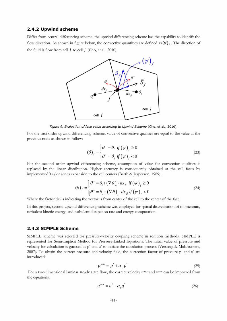
2.4.2 Upwind scheme

Differ from central differencing scheme, the upwind differencing scheme has the capability to identify the

flow direction. As shown in figure below, the convective quantities are defined as ( ) f . The direction of

the fluid is flow from cell i to cell j (Cho, et al., 2010).

Figure 9, Evaluation of face value according to Upwind Scheme (Cho, et al., 2010).

For the first order upwind differencing scheme, value of convective qualities are equal to the value at the

previous node as shown in follow:

0( )

0

i f

f

j f

if

if

(23)

For the second order upwind differencing scheme, assumption of value for convection qualities is

replaced by the linear distribution. Higher accuracy is consequently obtained at the cell faces by

implemented Taylor series expansion to the cell centers (Barth & Jesperson, 1989):

0( )

0

fii i f

f

fjj j f

dx if

dx if

(24)

Where the factor dxf is indicating the vector is from center of the cell to the center of the face.

In this project, second upwind differencing scheme was employed for spatial discretization of momentum,

turbulent kinetic energy, and turbulent dissipation rate and energy computation.

2.4.3 SIMPLE Scheme

SIMPLE scheme was selected for pressure-velocity coupling scheme in solution methods. SIMPLE is

represented for Semi-Implicit Method for Pressure-Linked Equations. The initial value of pressure and

velocity for calculation is guessed as p* and u* to initiate the calculation process (Versteeg & Malalasekera,

2007). To obtain the correct pressure and velocity field, the correction factor of pressure p’ and u’ are

introduced:

* 'new

pp p p (25)

For a two-dimensional laminar steady state flow, the correct velocity unew and vnew can be improved from

the equations:

* 'new

uu u u (26)

-12-

* 'new

vv v v (27)

The defined as under-relaxation factor for iterated calculation. This factor which taken from 0 to 1

helps to improve the iterative process move forward while influence the stability of the fluid flow

calculation. If the under-relaxation factor equal to zero, there will be no correction applied to the

computation. If the under-relaxation factor equal to one, the guessed field of pressure and velocity is far

away from the final solution.

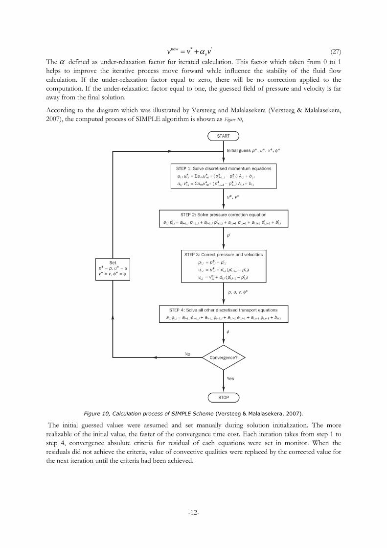
According to the diagram which was illustrated by Versteeg and Malalasekera (Versteeg & Malalasekera,

2007), the computed process of SIMPLE algorithm is shown as Figure 10,

Figure 10, Calculation process of SIMPLE Scheme (Versteeg & Malalasekera, 2007).

The initial guessed values were assumed and set manually during solution initialization. The more

realizable of the initial value, the faster of the convergence time cost. Each iteration takes from step 1 to

step 4, convergence absolute criteria for residual of each equations were set in monitor. When the

residuals did not achieve the criteria, value of convective qualities were replaced by the corrected value for

the next iteration until the criteria had been achieved.

-13-

3 Baseline model and Comparison between Software

In this chapter, baseline model would be initially built by ANSYS Fluent. According to ventilation system

had been implemented on ambulance hall of NKS (Nya Karolinska Solna) hospital, similar design concept

would be applied on the baseline model of the SÖS (Södersjukhuset) ambulance hall. Baseline models

which set up by IES VE – Microflo and Star – CCM+ were also discussed later in this chapter.

3.1 Data of ventilation system for baseline model.

3.1.1 Design Concept

According to requirements of design which supplied by the constructor of NKS hospital, the minimum

indoor air temperature of an ambulance hall which located in Stockholm, Sweden is not allowed be lower

than 18 and the air flow level should not lower than 3 l/s-m2.

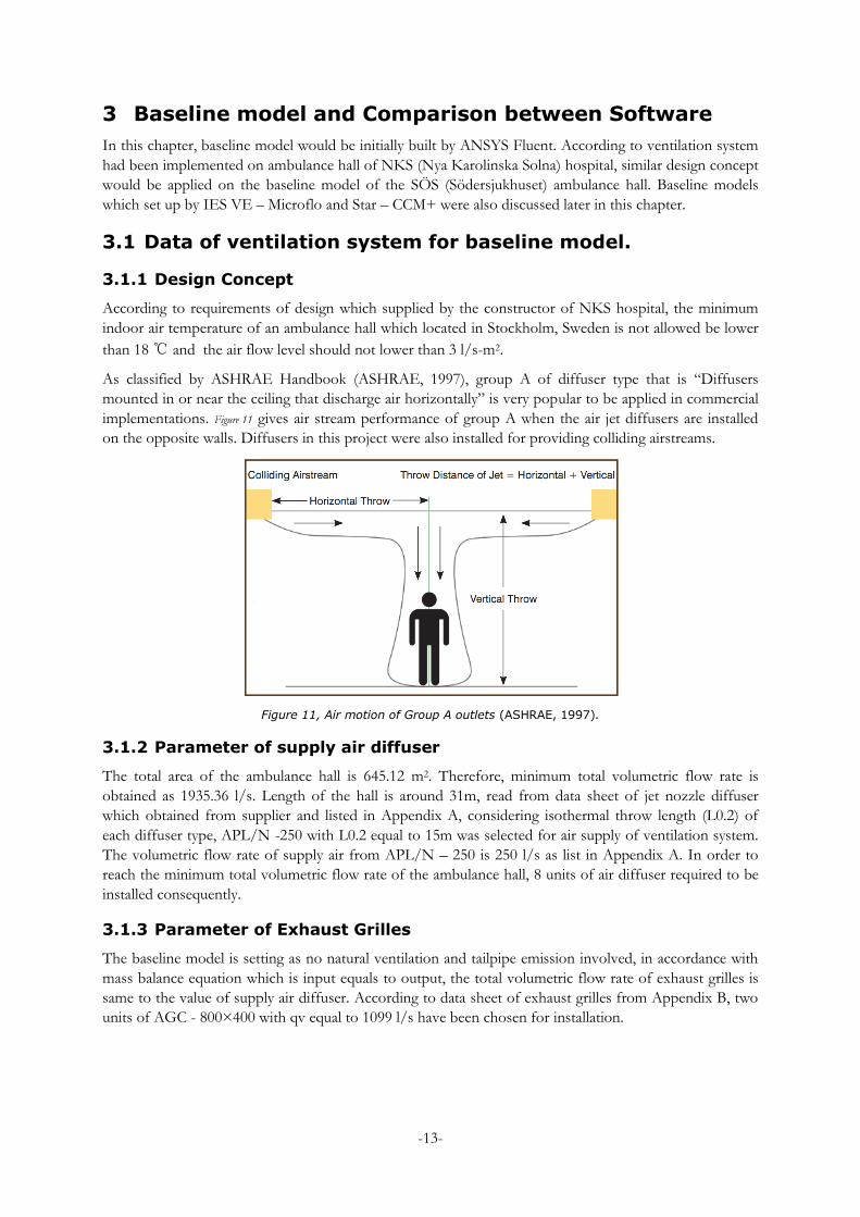
As classified by ASHRAE Handbook (ASHRAE, 1997), group A of diffuser type that is “Diffusers

mounted in or near the ceiling that discharge air horizontally” is very popular to be applied in commercial

implementations. Figure 11 gives air stream performance of group A when the air jet diffusers are installed

on the opposite walls. Diffusers in this project were also installed for providing colliding airstreams.

Figure 11, Air motion of Group A outlets (ASHRAE, 1997).

3.1.2 Parameter of supply air diffuser

The total area of the ambulance hall is 645.12 m2. Therefore, minimum total volumetric flow rate is

obtained as 1935.36 l/s. Length of the hall is around 31m, read from data sheet of jet nozzle diffuser

which obtained from supplier and listed in Appendix A, considering isothermal throw length (L0.2) of

each diffuser type, APL/N -250 with L0.2 equal to 15m was selected for air supply of ventilation system.

The volumetric flow rate of supply air from APL/N – 250 is 250 l/s as list in Appendix A. In order to

reach the minimum total volumetric flow rate of the ambulance hall, 8 units of air diffuser required to be

installed consequently.

3.1.3 Parameter of Exhaust Grilles

The baseline model is setting as no natural ventilation and tailpipe emission involved, in accordance with

mass balance equation which is input equals to output, the total volumetric flow rate of exhaust grilles is

same to the value of supply air diffuser. According to data sheet of exhaust grilles from Appendix B, two

units of AGC - 800×400 with qv equal to 1099 l/s have been chosen for installation.

-14-

3.2 Geometry

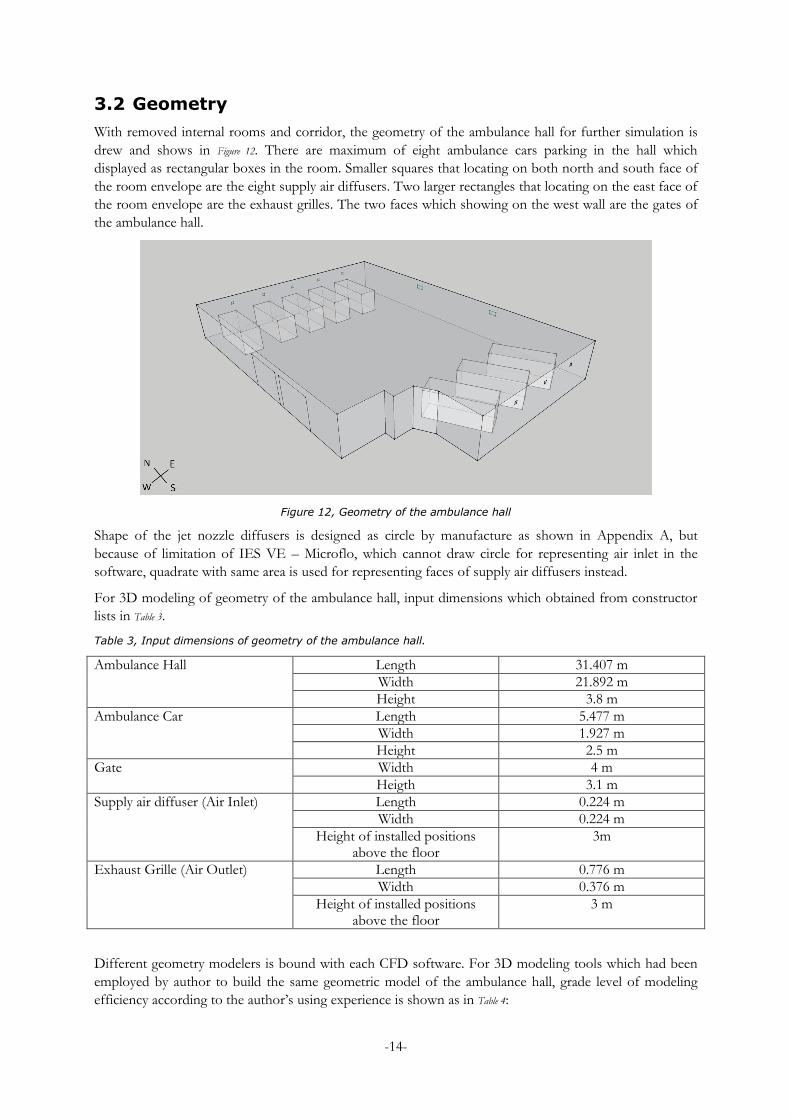
With removed internal rooms and corridor, the geometry of the ambulance hall for further simulation is

drew and shows in Figure 12. There are maximum of eight ambulance cars parking in the hall which

displayed as rectangular boxes in the room. Smaller squares that locating on both north and south face of

the room envelope are the eight supply air diffusers. Two larger rectangles that locating on the east face of

the room envelope are the exhaust grilles. The two faces which showing on the west wall are the gates of

the ambulance hall.

Figure 12, Geometry of the ambulance hall

Shape of the jet nozzle diffusers is designed as circle by manufacture as shown in Appendix A, but

because of limitation of IES VE – Microflo, which cannot draw circle for representing air inlet in the

software, quadrate with same area is used for representing faces of supply air diffusers instead.

For 3D modeling of geometry of the ambulance hall, input dimensions which obtained from constructor

lists in Table 3.

Table 3, Input dimensions of geometry of the ambulance hall.

Ambulance Hall Length 31.407 m

Width 21.892 m

Height 3.8 m

Ambulance Car Length 5.477 m

Width 1.927 m

Height 2.5 m

Gate Width 4 m

Heigth 3.1 m

Supply air diffuser (Air Inlet) Length 0.224 m

Width 0.224 m

Height of installed positions above the floor

3m

Exhaust Grille (Air Outlet) Length 0.776 m

Width 0.376 m

Height of installed positions above the floor

3 m

Different geometry modelers is bound with each CFD software. For 3D modeling tools which had been

employed by author to build the same geometric model of the ambulance hall, grade level of modeling

efficiency according to the author’s using experience is shown as in Table 4:

-15-

Table 4, Performance of 3D modeling for different tools.

3D Modeling

ANSYS Fluent IES VE - Microflo Star – CCM+

Tools DesigeModeller (Default)

SpaceClaim (collaborate)

ModelIT (Default)

SketchUp (Plug-In)

3D-CAD (Default)

SpaceClaim (export .stp

file )

Manipulate Difficulty of

Interface

3 5 1 4 2 5

Degree of precision

3 5 1 4 2 5

Time Spending

3 4 1 5 2 4

In Table 4, software performance is divided into 5 level. 3D modeling tool with the best efficiency and

performance gained 5 point, on the contrary, tools with less satisfaction are gained lower points. From

results of comparison, the geometry modeling tools of ANSYS has the capability to performance easier,

more intuitively and faster than the rest. Since the main functions of IES VE is to establish energy

performance for buildings, ModelIT is easier to be used for build building block without complex

geometry.

During simulation of baseline models, both ANSYS Fluent and Star – CCM+ shared same geometry file

which built by SpaceClaim, and SketchUp 2014 was employed for 3D modeling to IES VE – Microflo.

3.3 Meshing

3.3.1 Meshing Independency

Before continue with different circumstances of the ambulance hall, meshing independency study of

baseline scenario is strongly recommended to be implemented for obtain a more confident simulated

results. Therefore, two simulations of case 1.1, which is the baseline model modeled by ANSYS Fluent,

were generated as different number of cells. One with 380587 cell elements, the other one has 505743 cell

elements.

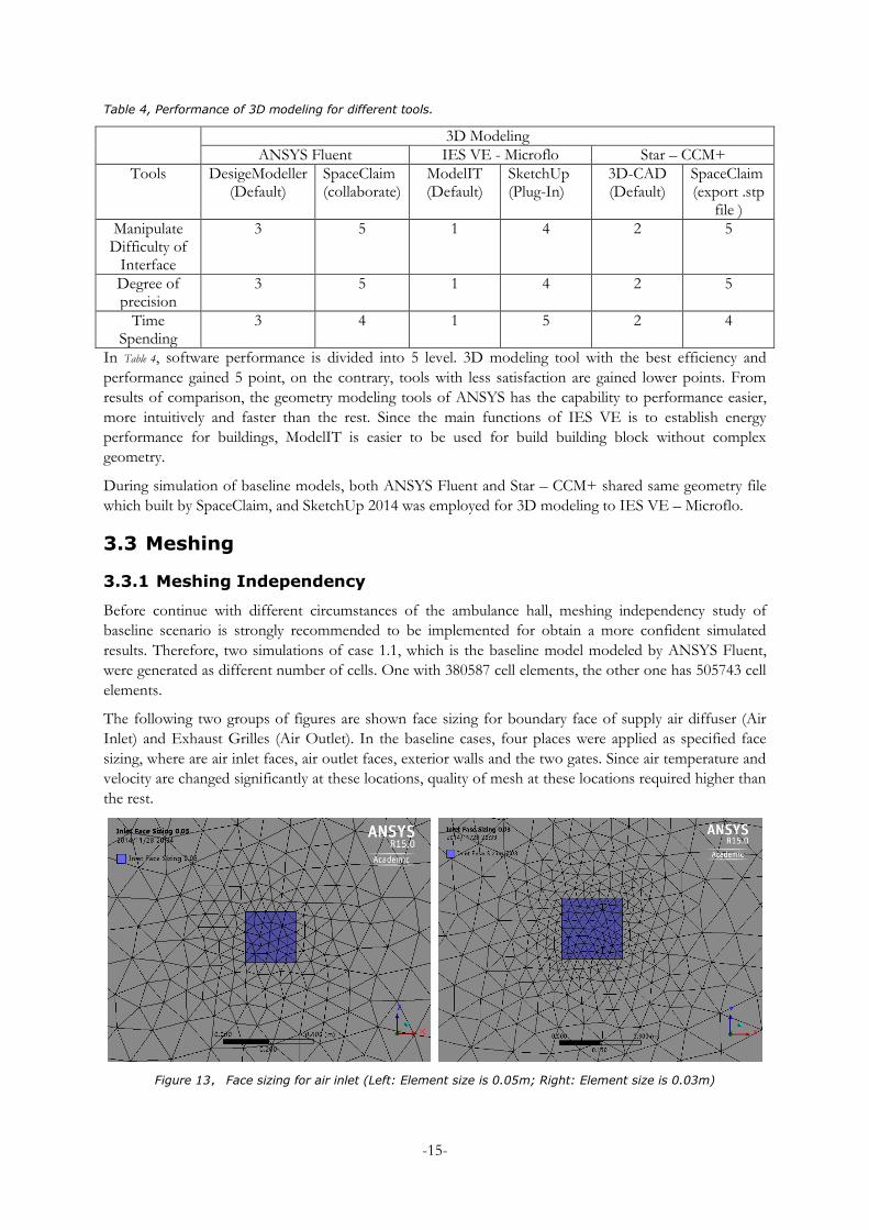
The following two groups of figures are shown face sizing for boundary face of supply air diffuser (Air

Inlet) and Exhaust Grilles (Air Outlet). In the baseline cases, four places were applied as specified face

sizing, where are air inlet faces, air outlet faces, exterior walls and the two gates. Since air temperature and

velocity are changed significantly at these locations, quality of mesh at these locations required higher than

the rest.

Figure 13， Face sizing for air inlet (Left: Element size is 0.05m; Right: Element size is 0.03m)

-16-

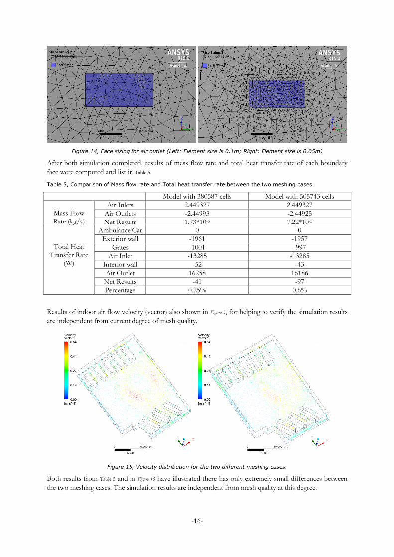
Figure 14, Face sizing for air outlet (Left: Element size is 0.1m; Right: Element size is 0.05m)

After both simulation completed, results of mess flow rate and total heat transfer rate of each boundary

face were computed and list in Table 5.

Table 5, Comparison of Mass flow rate and Total heat transfer rate between the two meshing cases

Model with 380587 cells Model with 505743 cells

Mass Flow Rate (kg/s)

Air Inlets 2.449327 2.449327

Air Outlets -2.44993 -2.44925

Net Results 1.73*10-5 7.22*10-5

Total Heat Transfer Rate

(W)

Ambulance Car 0 0

Exterior wall -1961 -1957

Gates -1001 -997

Air Inlet -13285 -13285

Interior wall -52 -43

Air Outlet 16258 16186

Net Results -41 -97

Percentage 0.25% 0.6%

Results of indoor air flow velocity (vector) also shown in Figure 3, for helping to verify the simulation results

are independent from current degree of mesh quality.

Figure 15, Velocity distribution for the two different meshing cases.

Both results from Table 5 and in Figure 15 have illustrated there has only extremely small differences between

the two meshing cases. The simulation results are independent from mesh quality at this degree.

-17-

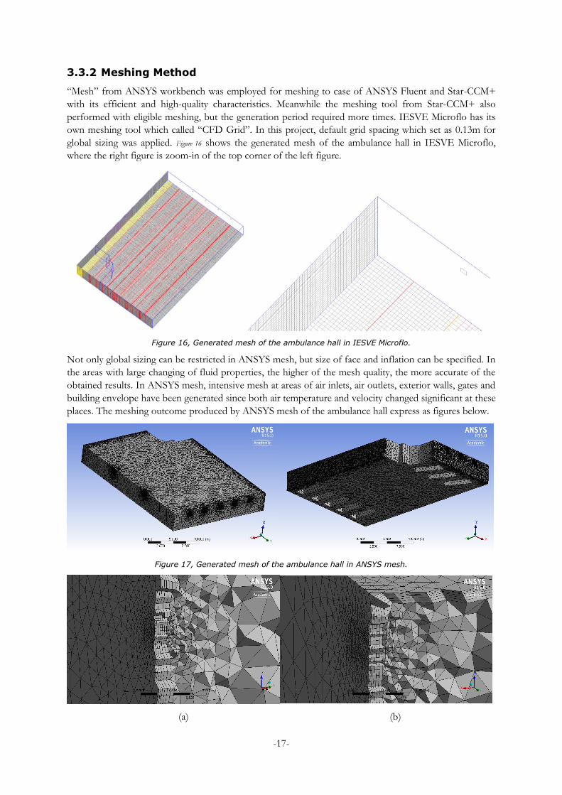
3.3.2 Meshing Method

“Mesh” from ANSYS workbench was employed for meshing to case of ANSYS Fluent and Star-CCM+

with its efficient and high-quality characteristics. Meanwhile the meshing tool from Star-CCM+ also

performed with eligible meshing, but the generation period required more times. IESVE Microflo has its

own meshing tool which called “CFD Grid”. In this project, default grid spacing which set as 0.13m for

global sizing was applied. Figure 16 shows the generated mesh of the ambulance hall in IESVE Microflo,

where the right figure is zoom-in of the top corner of the left figure.

Figure 16, Generated mesh of the ambulance hall in IESVE Microflo.

Not only global sizing can be restricted in ANSYS mesh, but size of face and inflation can be specified. In

the areas with large changing of fluid properties, the higher of the mesh quality, the more accurate of the

obtained results. In ANSYS mesh, intensive mesh at areas of air inlets, air outlets, exterior walls, gates and

building envelope have been generated since both air temperature and velocity changed significant at these

places. The meshing outcome produced by ANSYS mesh of the ambulance hall express as figures below.

Figure 17, Generated mesh of the ambulance hall in ANSYS mesh.

(a) (b)

-18-

(c) (d)

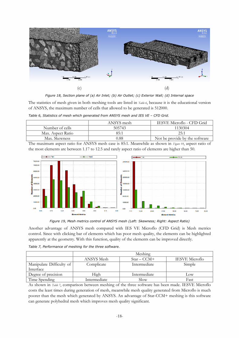
Figure 18, Section plane of (a) Air Inlet; (b) Air Outlet; (c) Exterior Wall; (d) Internal space

The statistics of mesh given in both meshing tools are listed in Table 6, because it is the educational version

of ANSYS, the maximum number of cells that allowed to be generated is 512000.

Table 6, Statistics of mesh which generated from ANSYS mesh and IES VE – CFD Grid.

ANSYS mesh IESVE Microflo - CFD Grid

Number of cells 505743 1130304

Max. Aspect Ratio 85:1 25:1

Max. Skewness 0.88 Not be provide by the software

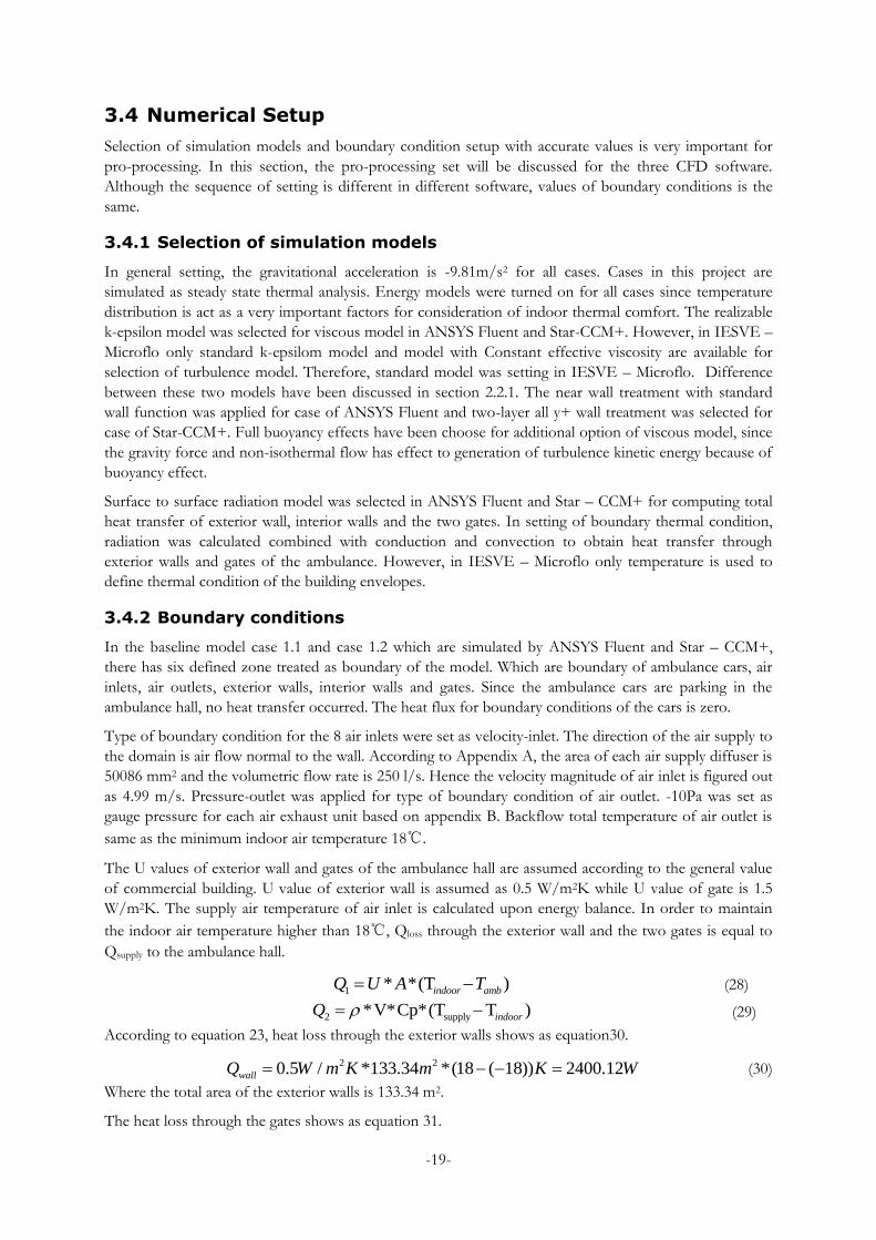
The maximum aspect ratio for ANSYS mesh case is 85:1. Meanwhile as shown in Figure 19, aspect ratio of

the most elements are between 1.17 to 12.5 and rarely aspect ratio of elements are higher than 50.

Figure 19, Mesh metrics control of ANSYS mesh (Left: Skewness; Right: Aspect Ratio)

Another advantage of ANSYS mesh compared with IES VE Microflo (CFD Grid) is Mesh metrics

control. Since with clicking bar of elements which has poor mesh quality, the elements can be highlighted

apparently at the geometry. With this function, quality of the elements can be improved directly.

Table 7, Performance of meshing for the three software.

Meshing

ANSYS Mesh Star – CCM+ IESVE Microflo

Manipulate Difficulty of Interface

Complicate Intermediate Simple

Degree of precision High Intermediate Low

Time Spending Intermediate Slow Fast

As shown in Table 7, comparison between meshing of the three software has been made. IESVE Microflo

costs the least times during generation of mesh, meanwhile mesh quality generated from Microflo is much

poorer than the mesh which generated by ANSYS. An advantage of Star-CCM+ meshing is this software

can generate polyhedral mesh which improves mesh quality significant.

-19-

3.4 Numerical Setup

Selection of simulation models and boundary condition setup with accurate values is very important for

pro-processing. In this section, the pro-processing set will be discussed for the three CFD software.

Although the sequence of setting is different in different software, values of boundary conditions is the

same.

3.4.1 Selection of simulation models

In general setting, the gravitational acceleration is -9.81m/s2 for all cases. Cases in this project are

simulated as steady state thermal analysis. Energy models were turned on for all cases since temperature

distribution is act as a very important factors for consideration of indoor thermal comfort. The realizable

k-epsilon model was selected for viscous model in ANSYS Fluent and Star-CCM+. However, in IESVE –

Microflo only standard k-epsilom model and model with Constant effective viscosity are available for

selection of turbulence model. Therefore, standard model was setting in IESVE – Microflo. Difference

between these two models have been discussed in section 2.2.1. The near wall treatment with standard

wall function was applied for case of ANSYS Fluent and two-layer all y+ wall treatment was selected for

case of Star-CCM+. Full buoyancy effects have been choose for additional option of viscous model, since

the gravity force and non-isothermal flow has effect to generation of turbulence kinetic energy because of

buoyancy effect.

Surface to surface radiation model was selected in ANSYS Fluent and Star – CCM+ for computing total

heat transfer of exterior wall, interior walls and the two gates. In setting of boundary thermal condition,

radiation was calculated combined with conduction and convection to obtain heat transfer through

exterior walls and gates of the ambulance. However, in IESVE – Microflo only temperature is used to

define thermal condition of the building envelopes.

3.4.2 Boundary conditions

In the baseline model case 1.1 and case 1.2 which are simulated by ANSYS Fluent and Star – CCM+,

there has six defined zone treated as boundary of the model. Which are boundary of ambulance cars, air

inlets, air outlets, exterior walls, interior walls and gates. Since the ambulance cars are parking in the

ambulance hall, no heat transfer occurred. The heat flux for boundary conditions of the cars is zero.

Type of boundary condition for the 8 air inlets were set as velocity-inlet. The direction of the air supply to

the domain is air flow normal to the wall. According to Appendix A, the area of each air supply diffuser is

50086 mm2 and the volumetric flow rate is 250 l/s. Hence the velocity magnitude of air inlet is figured out

as 4.99 m/s. Pressure-outlet was applied for type of boundary condition of air outlet. -10Pa was set as

gauge pressure for each air exhaust unit based on appendix B. Backflow total temperature of air outlet is

same as the minimum indoor air temperature 18.

The U values of exterior wall and gates of the ambulance hall are assumed according to the general value

of commercial building. U value of exterior wall is assumed as 0.5 W/m2K while U value of gate is 1.5

W/m2K. The supply air temperature of air inlet is calculated upon energy balance. In order to maintain

the indoor air temperature higher than 18, Qloss through the exterior wall and the two gates is equal to

Qsupply to the ambulance hall.

1 * *(T )indoor ambQ U A T (28)

2 supply*V*Cp*(T T )indoorQ (29)

According to equation 23, heat loss through the exterior walls shows as equation30.

2 20.5 / *133.34 *(18 ( 18)) 2400.12wallQ W m K m K W (30)

Where the total area of the exterior walls is 133.34 m2.

The heat loss through the gates shows as equation 31.

-20-

2 21.5 / *25.98 *(18 ( 18)) 1402.92gateQ W m K m K W (31)

Where the total area of the two gates are 25.98m2.

Hence, the total heat loss of the ambulance hall for indoor to ambient environment shows as equation 32.

2400.12 1402.92 3803.04Total wall gateQ Q Q W W W (32)

Finally, the supply temperature of air inlet is computed according to equation 24 shows as equation 33.

3 3

supply3803.04 1.225 / *2 / *1.0063*( 18)W kg m m s T

supply 19.543T .

(33)

In summary, the boundary conditions set up in ANSYS Fluent and Star-CCM+ are shown as in Table 8.

Table 8, Boundary Conditions set up in ANSYS Fluent and Star - CCM+.

Air Inlet (Velocity Inlet)

Velocity Specification Method Magnitude, Normal to Boundary Velocity Magnitude (m/s) 4.99 Turbulent Intensity (%) 5 Turbulent Viscosity Ratio 5 Temperature (C) 19.543 Air Outlet (Pressure-Outlet)

Gauge Pressure (Pascal) -10 Backflow Direction Specification Method Normal to Boundary Backflow Total Temperature (C) 18 Exterior Walls (Wall)

Wall Motion Stationary Wall Thermal Conditions Mixed External Heat Transfer Coefficient (w/m2-k) 25 Free Stream Temperature (C) -18 External Emissivity 0.9 External Radiation Temperature (C) -18 Internal Emissivity 0.9 Wall Thickness (m) 0.4 S2S Faces per Surface Cluster 10 U value 0.5 W/m2K Interior Walls(Wall)

Wall Motion Stationary Wall Thermal Conditions Radiation External Emissivity 0.9 External Radiation Temperature (C) 18 Internal Emissivity 0.9 Wall Thickness(m) 0.2 S2S Faces per Surface Cluster 10 Gate (Wall)

Thermal Conditions Mixed External Heat Transfer Coefficient (w/m2-k) 25 Free Stream Temperature (C) -18 External Emissivity 0.9 External Radiation Temperature (C) -18 Internal Emissivity 0.9 Thickness (m) 0.2 S2S Faces per Surface Cluster 10 U value 1.5W/m2K Ambulance Cars(Wall)

Thermal Conditions Heat Flux Heat Flux (w/m2) 0

-21-

Differ from thermal properties setting in ANSYS Fluent, thermal resistance (R-value) of exterior walls and

gates were implied in Star-CCM+ instead of thermal conductivity (U-value). Therefore, thermal resistance

2 m2K/W of exterior walls and 0.67 m2K/W of gates were input for calculation of heat loss through the

building envelope of the ambulance hall.

The boundary condition setting process is completely different in IESVE Microflo. The thermal

properties of building envelopes were edited in IESVE ModelBuilder. It is another application which

included in IESVE workbench. The U-value of building envelopes were set up with building geometry

simultaneously in IESVE ModelIT. After modification in APlocate, data of weather for the building

location was downloaded from ASHRAE design weather database v4.0. Therefore, the annual dry-bulb

and wet-bulb temperature of Stockholm, where the ambulance hall located, had been obtained as outdoor

temperature for computing heat transfer through the walls and gates.

For drawing of boundary conditions of air inlet and outlet, only shapes of rectangular and polygonal are

validate for add these kind of boundaries after complication of building geometry. The supply air with

velocity inlet and exhaust air with pressure outlet were applied in IESVE Microflo which all the values are

same as setting in the previous two software.

The thermal conditions of exterior walls, interior walls and gates are selected with Mixed and Radiation in

ANSYS Fluent and Star-CCM+ as shown in Table 8, but considering thermal conditions of building

envelopes in IESVE Microflo only Default Surface Temperature (C) is available for the heat loss

calculation. Here in the baseline case 1.3 which the model built in Microflo, 18 as surface temperature

was set in CFD settings.

3.4.3 Solution Control

As discussed in section 2.4, SIMPLE scheme as pressure-velocity coupling scheme was selected for

solution method in ANSYS Fluent. With higher order accuracy, second order upwind scheme was

employed for spatial discretization of momentum, turbulent kinetic energy, and turbulent dissipation rate

and energy of the indoor fluid in ANSYS FLUENT. Same as coupled model in Fluent, IESVE Microflo is

also implied pressure-velocity coupled model of fluid flow.

Unlike the other two software, case 1.2 which simulated in Star – CCM+ was used segregated flow. Since

for most of cases which does not have problem of supersonic flow, segregated flow can saved more

computational time and memories, but on contrary it might be unstable. Combined with segregated flow

model, segregated fluid temperature model which solves energy equation with temperature as the variable

(CD-adapco, 2013).

In summary, solution control of the three software is illustrated as in Table 9. The under-relaxation factors

( ) of the convective properties also shows in the table. Because of educational version of ANSYS

Fluent, mesh quality of the case 1.1 did not reached the optimized. Hence, in order to converge the

residual with less iteration, lower under-relaxation factors had been set.

-22-

Table 9, Solution control for the three software.

ANSYS Fluent Star-CCM+ IESVE Microflo

Solution Methods Pressure-Velocity Coupled Flow (SIMPLE Scheme)

Segregated Flow Model Coupled Flow Model

Discretization Scheme Upwind Second Order Segregated Temperature Upwind First Order

of Pressure 0.3 0.3 -

of Velocity - 0.7 0.1

of Density 1 - -

of Momentum 0.7 - -

of Turbulent Kinetic Energy

0.2 0.8 0.05

of Turbulent Dissipation Rate

0.2 0.8 0.05

of Turbulent Viscosity

0.4 1 0.05

of Energy 0.9 0.9 1

The convergence absolute criteria of residual for case 1.1 in ANSYS Fluent is 1*10-4 for x-/y-/z-velocity.

And for the rest equations like continuity, energy, k and epsilon, 1*10-3 was set as residual convergence

criteria. For case 1.2 in Star-CCM+ and case 1.3 in IESVE Microflo, 1*10-4 was applied as the criteria.

Table 10, Performance of numerical setup for the three software.

Numerical Setup

ANSYS Fluent Star – CCM+ IESVE Microflo

Manipulate Difficulty of Interface

Complicate Intermediate Simple

Degree of precision High Intermediate Low

Compare with the other two CFD simulation software, ANSYS Fluent provides more selections of

schemes to adapt computations of variety fluid dynamics with higher precision. On contrary, IESVE

Microflo was specified designed to simulate environment of building for both internal and external

analysis with lower precision.

-23-

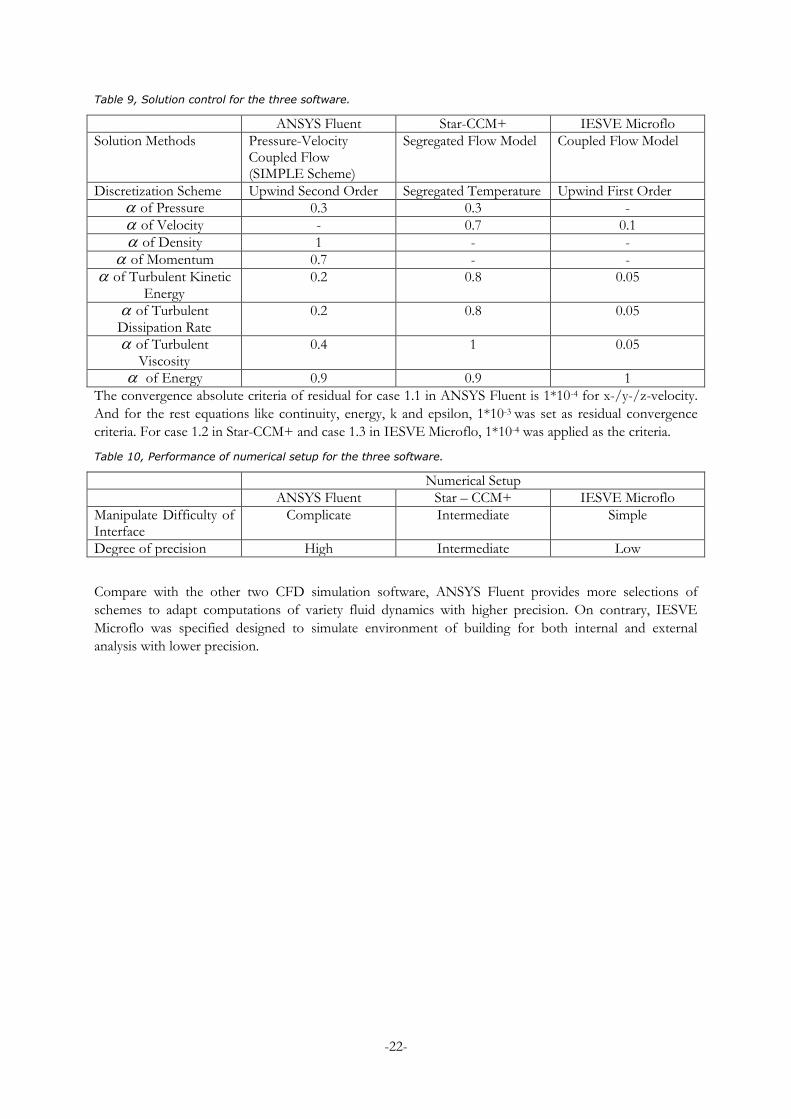
3.5 Simulation results

Baseline Case 1.1 and 1.2 which operated in ANSYS Fluent and Star-CCM+ have achieved the

convergence absolute criteria of residual. For case 1.3 which operated in IESVE Microflo, the

convergence absolute criteria of residual did not achieved below 1*10-4. However, according to cell

monitor at point (x=4.258m, y=15.702m, z=1.9m), results of each convective properties were turned into

steady state as shown in Figure 20. Therefore, result of simulation for case 1.3 with lower accuracy than the

others also be validated for practical application.

Figure 20, Cell Monitor of point in Case 1.3.

3.5.1 Assessment of thermal comfort in an arbitrary point.

According to ASHREA standard 55-1992 (McQuiston, et al., 2005), Predicated mean vote (PMV) is used

as thermal comfort index for assess the indoor environment thermal conditions. The scale of PMV is list

in Table 11.

Table 11, Thermal sensation scale for PMV Method.

Value +3 +2 +1 0 -1 -2 -3

Thermal Sensation

hot warm slightly warm

neutral slightly cool

cool cold

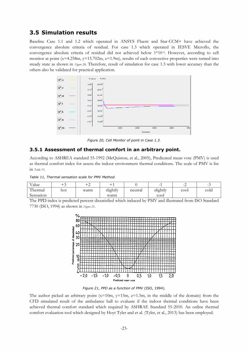
The PPD index is predicted percent dissatisfied which induced by PMV and illustrated from ISO Standard

7730 (ISO, 1994) as shown in Figure 21.

Figure 21, PPD as a function of PMV (ISO, 1994).

The author picked an arbitrary point (x=10m, y=15m, z=1.5m, in the middle of the domain) from the

CFD simulated result of the ambulance hall to evaluate if the indoor thermal conditions have been

achieved thermal comfort standard which required by ASHRAE Standard 55-2010. An online thermal

comfort evaluation tool which designed by Hoyt Tyler and et al. (Tyler, et al., 2013) has been employed.

-24-

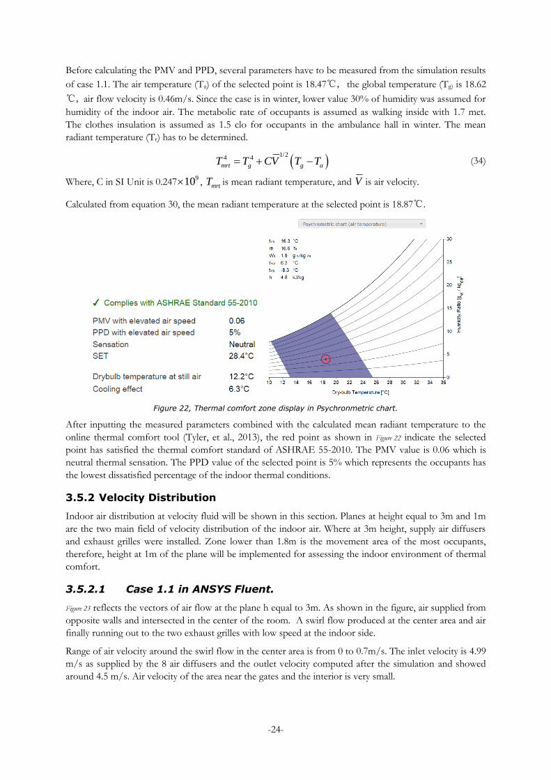
Before calculating the PMV and PPD, several parameters have to be measured from the simulation results

of case 1.1. The air temperature (Ta) of the selected point is 18.47, the global temperature (Tg) is 18.62

, air flow velocity is 0.46m/s. Since the case is in winter, lower value 30% of humidity was assumed for

humidity of the indoor air. The metabolic rate of occupants is assumed as walking inside with 1.7 met.

The clothes insulation is assumed as 1.5 clo for occupants in the ambulance hall in winter. The mean

radiant temperature (Tr) has to be determined.

1/2

4 4

mrt g g aT T CV T T (34)

Where, C in SI Unit is 0.247910 ,

mrtT is mean radiant temperature, and V is air velocity.

Calculated from equation 30, the mean radiant temperature at the selected point is 18.87.

Figure 22, Thermal comfort zone display in Psychronmetric chart.

After inputting the measured parameters combined with the calculated mean radiant temperature to the

online thermal comfort tool (Tyler, et al., 2013), the red point as shown in Figure 22 indicate the selected

point has satisfied the thermal comfort standard of ASHRAE 55-2010. The PMV value is 0.06 which is

neutral thermal sensation. The PPD value of the selected point is 5% which represents the occupants has

the lowest dissatisfied percentage of the indoor thermal conditions.

3.5.2 Velocity Distribution

Indoor air distribution at velocity fluid will be shown in this section. Planes at height equal to 3m and 1m

are the two main field of velocity distribution of the indoor air. Where at 3m height, supply air diffusers

and exhaust grilles were installed. Zone lower than 1.8m is the movement area of the most occupants,

therefore, height at 1m of the plane will be implemented for assessing the indoor environment of thermal

comfort.

3.5.2.1 Case 1.1 in ANSYS Fluent.

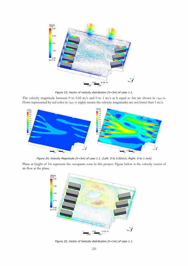
Figure 23 reflects the vectors of air flow at the plane h equal to 3m. As shown in the figure, air supplied from

opposite walls and intersected in the center of the room. A swirl flow produced at the center area and air

finally running out to the two exhaust grilles with low speed at the indoor side.

Range of air velocity around the swirl flow in the center area is from 0 to 0.7m/s. The inlet velocity is 4.99

m/s as supplied by the 8 air diffusers and the outlet velocity computed after the simulation and showed

around 4.5 m/s. Air velocity of the area near the gates and the interior is very small.

-25-

Figure 23, Vector of velocity distribution (h=3m) of case 1.1.

The velocity magnitude between 0 to 5.02 m/s and 0 to 1 m/s at h equal to 3m are shown in Figure 24.

Flows represented by red color in Figure 24 (right) means the velocity magnitudes are not lower than 1 m/s.

Figure 24, Velocity Magnitude (h=3m) of case 1.1. (Left: 0 to 5.02m/s, Right: 0 to 1 m/s)

Plane at height of 1m represent the occupants zone in this project. Figure below is the velocity vector of

air flow at the plane.

Figure 25, Vector of Velocity distribution (h=1m) of case 1.1.

-26-

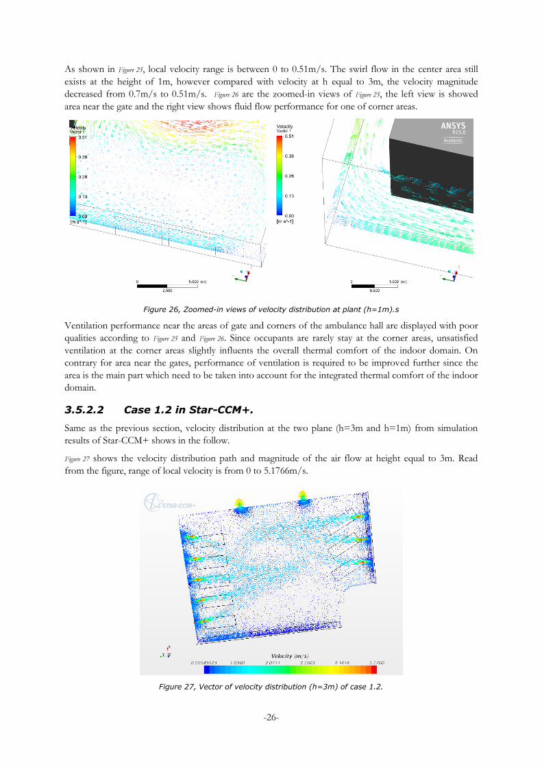
As shown in Figure 25, local velocity range is between 0 to 0.51m/s. The swirl flow in the center area still

exists at the height of 1m, however compared with velocity at h equal to 3m, the velocity magnitude

decreased from 0.7m/s to 0.51m/s. Figure 26 are the zoomed-in views of Figure 25, the left view is showed

area near the gate and the right view shows fluid flow performance for one of corner areas.

Figure 26, Zoomed-in views of velocity distribution at plant (h=1m).s

Ventilation performance near the areas of gate and corners of the ambulance hall are displayed with poor

qualities according to Figure 25 and Figure 26. Since occupants are rarely stay at the corner areas, unsatisfied

ventilation at the corner areas slightly influents the overall thermal comfort of the indoor domain. On

contrary for area near the gates, performance of ventilation is required to be improved further since the

area is the main part which need to be taken into account for the integrated thermal comfort of the indoor

domain.

3.5.2.2 Case 1.2 in Star-CCM+.

Same as the previous section, velocity distribution at the two plane (h=3m and h=1m) from simulation

results of Star-CCM+ shows in the follow.

Figure 27 shows the velocity distribution path and magnitude of the air flow at height equal to 3m. Read

from the figure, range of local velocity is from 0 to 5.1766m/s.

Figure 27, Vector of velocity distribution (h=3m) of case 1.2.

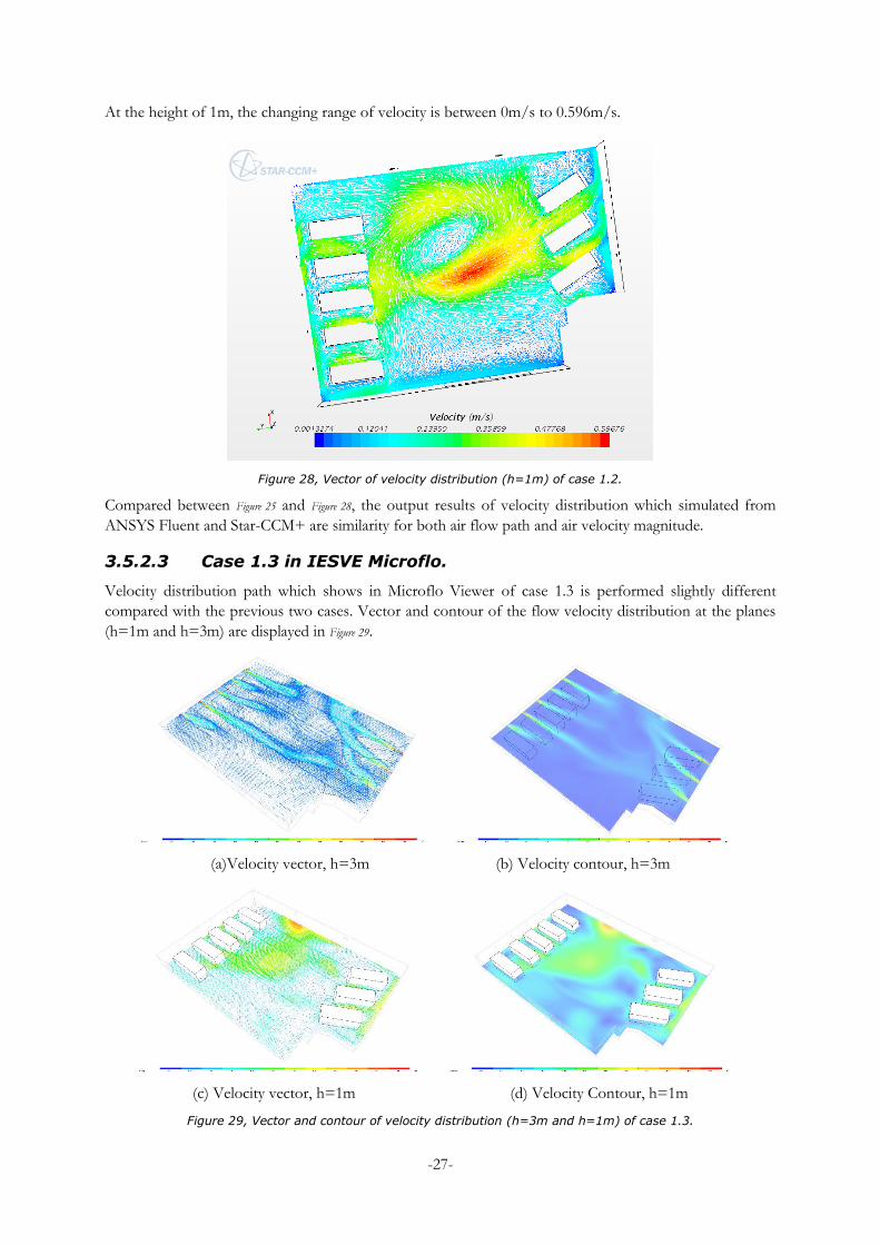
-27-

At the height of 1m, the changing range of velocity is between 0m/s to 0.596m/s.

Figure 28, Vector of velocity distribution (h=1m) of case 1.2.

Compared between Figure 25 and Figure 28, the output results of velocity distribution which simulated from

ANSYS Fluent and Star-CCM+ are similarity for both air flow path and air velocity magnitude.

3.5.2.3 Case 1.3 in IESVE Microflo.

Velocity distribution path which shows in Microflo Viewer of case 1.3 is performed slightly different

compared with the previous two cases. Vector and contour of the flow velocity distribution at the planes

(h=1m and h=3m) are displayed in Figure 29.

(a)Velocity vector, h=3m (b) Velocity contour, h=3m

(c) Velocity vector, h=1m (d) Velocity Contour, h=1m

Figure 29, Vector and contour of velocity distribution (h=3m and h=1m) of case 1.3.

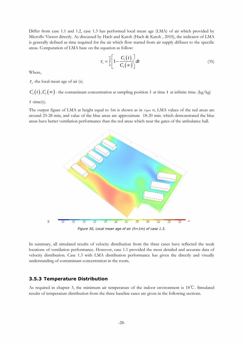
-28-

Differ from case 1.1 and 1.2, case 1.3 has performed local mean age (LMA) of air which provided by

Microflo Viewer directly. As discussed by Hach and Katoh (Hach & Katoh , 2010), the indicator of LMA

is generally defined as time required for the air which flow started from air supply diffuser to the specific

areas. Computation of LMA base on the equation as follow:

0

1i

i

i

C tdt

C

(35)

Where,

i -the local mean age of air (s).

iC t , iC - the contaminant concentration at sampling position i at time t at infinite time. (kg/kg)

t -time(s).

The output figure of LMA at height equal to 1m is shown as in Figure 30, LMA values of the red areas are

around 25-28 min, and value of the blue areas are approximate 18-20 min. which demonstrated the blue

areas have better ventilation performance than the red areas which near the gates of the ambulance hall.

Figure 30, Local mean age of air (h=1m) of case 1.3.

In summary, all simulated results of velocity distribution from the three cases have reflected the weak

locations of ventilation performance. However, case 1.1 provided the most detailed and accurate data of

velocity distribution. Case 1.3 with LMA distribution performance has given the directly and visually

understanding of contaminant concentration in the room.

3.5.3 Temperature Distribution

As required in chapter 3, the minimum air temperature of the indoor environment is 18. Simulated

results of temperature distribution from the three baseline cases are given in the following sections.

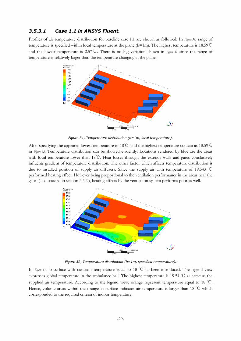
-29-

3.5.3.1 Case 1.1 in ANSYS Fluent.

Profiles of air temperature distribution for baseline case 1.1 are shown as followed. In Figure 31, range of

temperature is specified within local temperature at the plane (h=1m). The highest temperature is 18.59

and the lowest temperature is 2.57. There is no big variation shown in Figure 31 since the range of

temperature is relatively larger than the temperature changing at the plane.

Figure 31, Temperature distribution (h=1m, local temperature).

After specifying the appeared lowest temperature to 18 and the highest temperature contain as 18.59

in Figure 32. Temperature distribution can be showed evidently. Locations rendered by blue are the areas

with local temperature lower than 18. Heat losses through the exterior walls and gates conclusively

influents gradient of temperature distribution. The other factor which affects temperature distribution is

due to installed position of supply air diffusers. Since the supply air with temperature of 19.543

performed heating effect. However being proportional to the ventilation performance in the areas near the

gates (as discussed in section 3.5.2.), heating effects by the ventilation system performs poor as well.

Figure 32, Temperature distribution (h=1m, specified temperature).

In Figure 33, isosurface with constant temperature equal to 18 has been introduced. The legend view

expresses global temperature in the ambulance hall. The highest temperature is 19.54 as same as the

supplied air temperature. According to the legend view, orange represent temperature equal to 18 .

Hence, volume areas within the orange isosurface indicates air temperature is larger than 18 which

corresponded to the required criteria of indoor temperature.

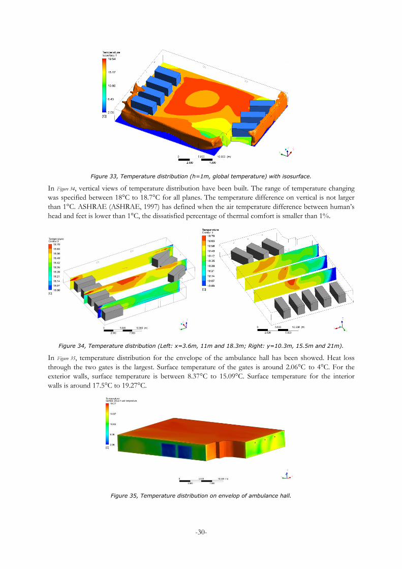
-30-

Figure 33, Temperature distribution (h=1m, global temperature) with isosurface.

In Figure 34, vertical views of temperature distribution have been built. The range of temperature changing

was specified between 18°C to 18.7°C for all planes. The temperature difference on vertical is not larger

than 1°C. ASHRAE (ASHRAE, 1997) has defined when the air temperature difference between human’s

head and feet is lower than 1°C, the dissatisfied percentage of thermal comfort is smaller than 1%.

Figure 34, Temperature distribution (Left: x=3.6m, 11m and 18.3m; Right: y=10.3m, 15.5m and 21m).

In Figure 35, temperature distribution for the envelope of the ambulance hall has been showed. Heat loss

through the two gates is the largest. Surface temperature of the gates is around 2.06°C to 4°C. For the

exterior walls, surface temperature is between 8.37°C to 15.09°C. Surface temperature for the interior

walls is around 17.5°C to 19.27°C.

Figure 35, Temperature distribution on envelop of ambulance hall.

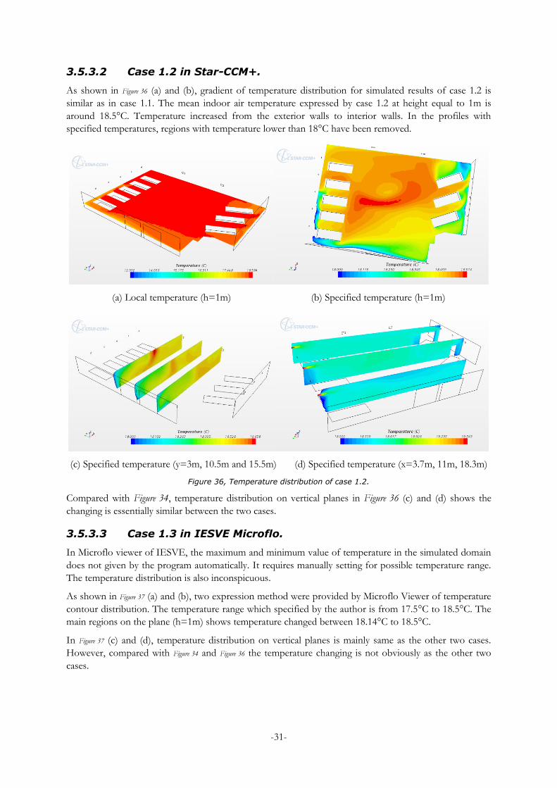
-31-

3.5.3.2 Case 1.2 in Star-CCM+.

As shown in Figure 36 (a) and (b), gradient of temperature distribution for simulated results of case 1.2 is

similar as in case 1.1. The mean indoor air temperature expressed by case 1.2 at height equal to 1m is

around 18.5°C. Temperature increased from the exterior walls to interior walls. In the profiles with

specified temperatures, regions with temperature lower than 18°C have been removed.

(a) Local temperature (h=1m) (b) Specified temperature (h=1m)

(c) Specified temperature (y=3m, 10.5m and 15.5m) (d) Specified temperature (x=3.7m, 11m, 18.3m)

Figure 36, Temperature distribution of case 1.2.

Compared with Figure 34, temperature distribution on vertical planes in Figure 36 (c) and (d) shows the

changing is essentially similar between the two cases.

3.5.3.3 Case 1.3 in IESVE Microflo.

In Microflo viewer of IESVE, the maximum and minimum value of temperature in the simulated domain

does not given by the program automatically. It requires manually setting for possible temperature range.

The temperature distribution is also inconspicuous.

As shown in Figure 37 (a) and (b), two expression method were provided by Microflo Viewer of temperature

contour distribution. The temperature range which specified by the author is from 17.5°C to 18.5°C. The

main regions on the plane (h=1m) shows temperature changed between 18.14°C to 18.5°C.

In Figure 37 (c) and (d), temperature distribution on vertical planes is mainly same as the other two cases.

However, compared with Figure 34 and Figure 36 the temperature changing is not obviously as the other two

cases.

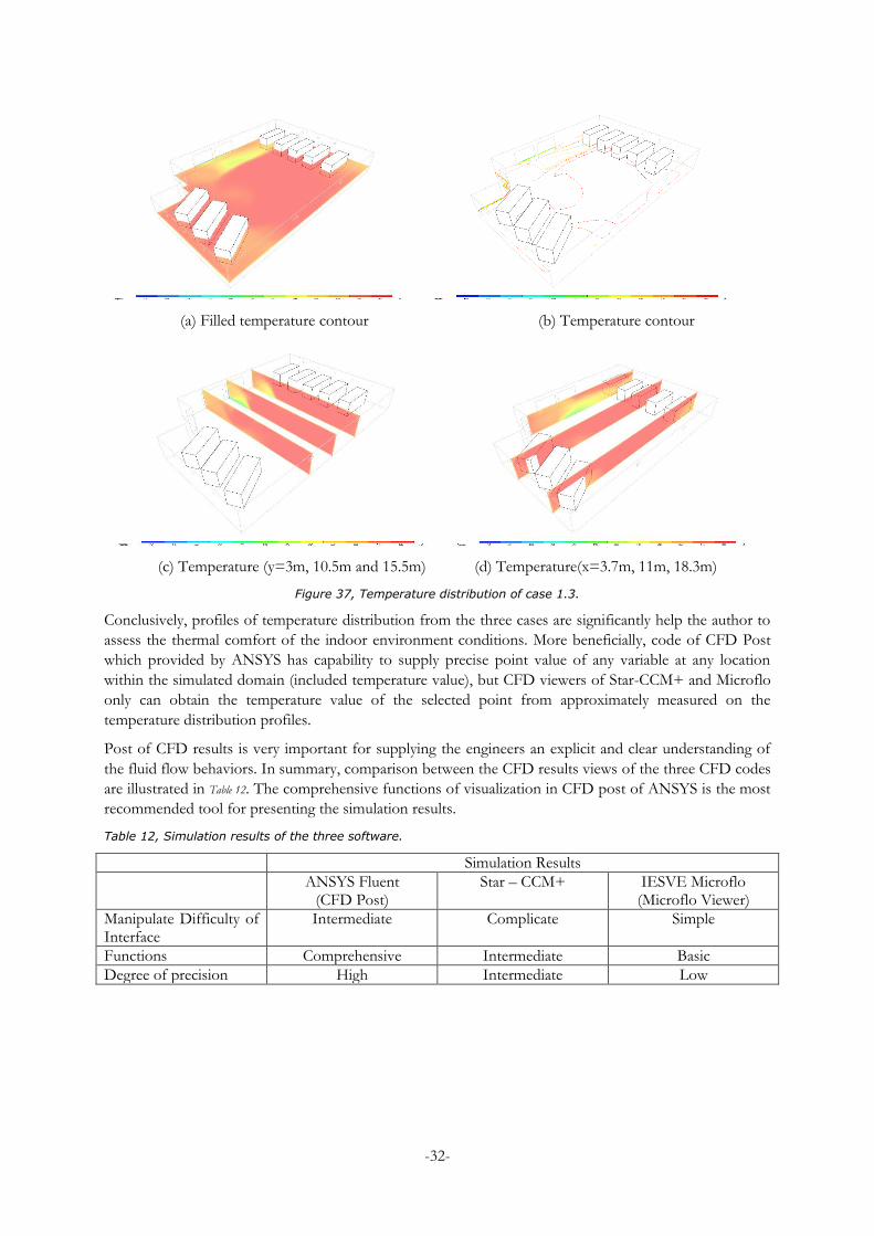
-32-

(a) Filled temperature contour (b) Temperature contour

(c) Temperature (y=3m, 10.5m and 15.5m) (d) Temperature(x=3.7m, 11m, 18.3m)

Figure 37, Temperature distribution of case 1.3.

Conclusively, profiles of temperature distribution from the three cases are significantly help the author to

assess the thermal comfort of the indoor environment conditions. More beneficially, code of CFD Post

which provided by ANSYS has capability to supply precise point value of any variable at any location

within the simulated domain (included temperature value), but CFD viewers of Star-CCM+ and Microflo

only can obtain the temperature value of the selected point from approximately measured on the

temperature distribution profiles.

Post of CFD results is very important for supplying the engineers an explicit and clear understanding of

the fluid flow behaviors. In summary, comparison between the CFD results views of the three CFD codes

are illustrated in Table 12. The comprehensive functions of visualization in CFD post of ANSYS is the most

recommended tool for presenting the simulation results.

Table 12, Simulation results of the three software.

Simulation Results

ANSYS Fluent (CFD Post)

Star – CCM+ IESVE Microflo (Microflo Viewer)

Manipulate Difficulty of Interface

Intermediate Complicate Simple

Functions Comprehensive Intermediate Basic

Degree of precision High Intermediate Low

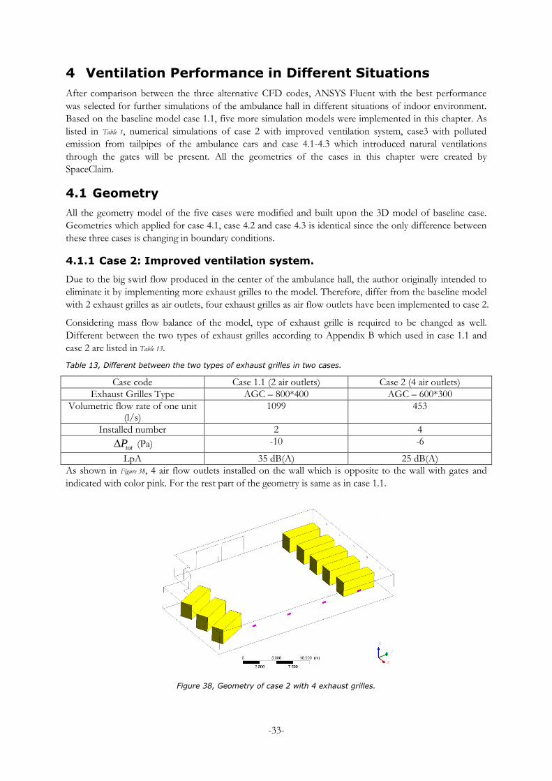
-33-

4 Ventilation Performance in Different Situations

After comparison between the three alternative CFD codes, ANSYS Fluent with the best performance

was selected for further simulations of the ambulance hall in different situations of indoor environment.

Based on the baseline model case 1.1, five more simulation models were implemented in this chapter. As

listed in Table 1, numerical simulations of case 2 with improved ventilation system, case3 with polluted

emission from tailpipes of the ambulance cars and case 4.1-4.3 which introduced natural ventilations

through the gates will be present. All the geometries of the cases in this chapter were created by

SpaceClaim.

4.1 Geometry

All the geometry model of the five cases were modified and built upon the 3D model of baseline case.

Geometries which applied for case 4.1, case 4.2 and case 4.3 is identical since the only difference between

these three cases is changing in boundary conditions.

4.1.1 Case 2: Improved ventilation system.

Due to the big swirl flow produced in the center of the ambulance hall, the author originally intended to

eliminate it by implementing more exhaust grilles to the model. Therefore, differ from the baseline model

with 2 exhaust grilles as air outlets, four exhaust grilles as air flow outlets have been implemented to case 2.

Considering mass flow balance of the model, type of exhaust grille is required to be changed as well.

Different between the two types of exhaust grilles according to Appendix B which used in case 1.1 and

case 2 are listed in Table 13.

Table 13, Different between the two types of exhaust grilles in two cases.

Case code Case 1.1 (2 air outlets) Case 2 (4 air outlets)

Exhaust Grilles Type AGC – 800*400 AGC – 600*300

Volumetric flow rate of one unit (l/s)

1099 453

Installed number 2 4

totP (Pa) -10 -6

LpA 35 dB(A) 25 dB(A)

As shown in Figure 38, 4 air flow outlets installed on the wall which is opposite to the wall with gates and

indicated with color pink. For the rest part of the geometry is same as in case 1.1.

Figure 38, Geometry of case 2 with 4 exhaust grilles.

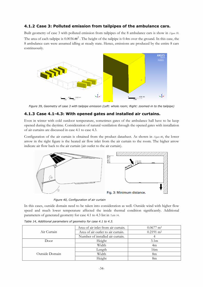
-34-

4.1.2 Case 3: Polluted emission from tailpipes of the ambulance cars.

Built geometry of case 3 with polluted emission from tailpipes of the 8 ambulance cars is show in Figure 39.

The area of each tailpipe is 0.00362m . The height of the tailpipe is 0.4m over the ground. In this case, the

8 ambulance cars were assumed idling at steady state. Hence, emissions are produced by the entire 8 cars

continuously.

Figure 39, Geometry of case 3 with tailpipe emission (Left: whole room; Right: zoomed-in to the tailpipe)

4.1.3 Case 4.1-4.3: With opened gates and installed air curtains.

Even in winter with cold outdoor temperature, sometimes gates of the ambulance hall have to be keep

opened during the daytime. Consideration of natural ventilation through the opened gates with installation

of air curtains are discussed in case 4.1 to case 4.3.

Configuration of the air curtain is obtained from the product datasheet. As shown in Figure 40, the lower

arrow in the right figure is the heated air flow inlet from the air curtain to the room. The higher arrow

indicate air flow back to the air curtain (air outlet to the air curtain).

Figure 40, Configuration of air curtain which installed in case 4.1-4.3.

In this cases, outside domain need to be taken into consideration as well. Outside wind with higher flow

speed and much lower temperature affected the inside thermal condition significantly. Additional

parameters of generated geometry for case 4.1 to 4.3 list in Table 14.

Table 14, Additional parameters of geometry for case 4.1 to 4.3.

Air Curtain

Area of air inlet from air curtain. 0.0677 m2

Area of air outlet to air curtain. 0.2191 m2

Number of installed air curtain. 4

Door Height 3.1m

Width 4m

Outside Domain

Length 16m

Width 8m

Height 8m

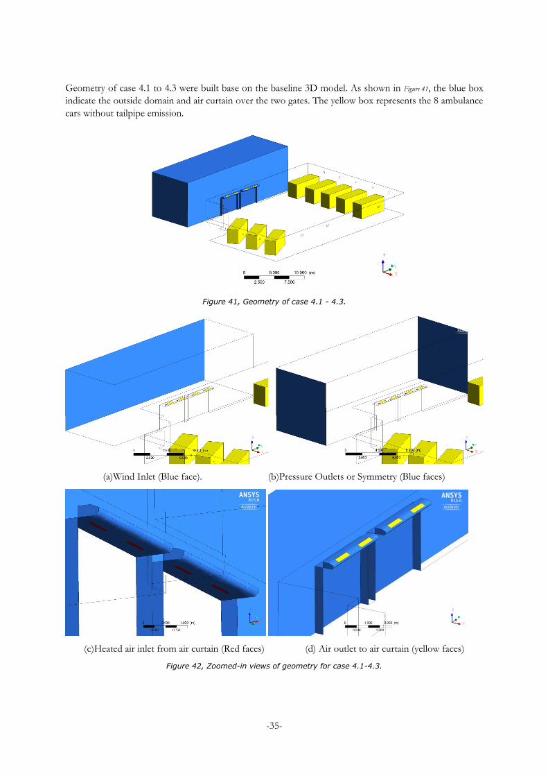
-35-

Geometry of case 4.1 to 4.3 were built base on the baseline 3D model. As shown in Figure 41, the blue box

indicate the outside domain and air curtain over the two gates. The yellow box represents the 8 ambulance

cars without tailpipe emission.

Figure 41, Geometry of case 4.1 - 4.3.

(a)Wind Inlet (Blue face). (b)Pressure Outlets or Symmetry (Blue faces)

(c)Heated air inlet from air curtain (Red faces) (d) Air outlet to air curtain (yellow faces)

Figure 42, Zoomed-in views of geometry for case 4.1-4.3.

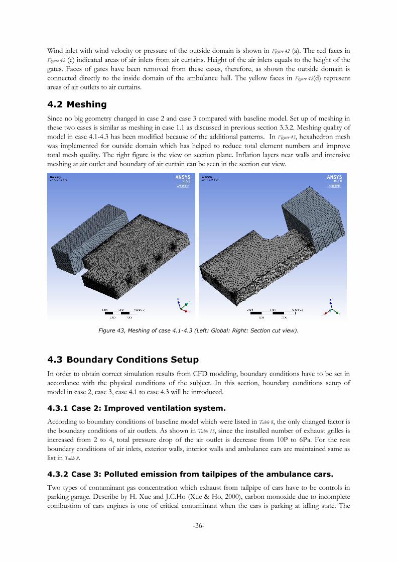
-36-

Wind inlet with wind velocity or pressure of the outside domain is shown in Figure 42 (a). The red faces in

Figure 42 (c) indicated areas of air inlets from air curtains. Height of the air inlets equals to the height of the

gates. Faces of gates have been removed from these cases, therefore, as shown the outside domain is

connected directly to the inside domain of the ambulance hall. The yellow faces in Figure 42(d) represent

areas of air outlets to air curtains.

4.2 Meshing

Since no big geometry changed in case 2 and case 3 compared with baseline model. Set up of meshing in

these two cases is similar as meshing in case 1.1 as discussed in previous section 3.3.2. Meshing quality of

model in case 4.1-4.3 has been modified because of the additional patterns. In Figure 43, hexahedron mesh

was implemented for outside domain which has helped to reduce total element numbers and improve

total mesh quality. The right figure is the view on section plane. Inflation layers near walls and intensive

meshing at air outlet and boundary of air curtain can be seen in the section cut view.

Figure 43, Meshing of case 4.1-4.3 (Left: Global: Right: Section cut view).

4.3 Boundary Conditions Setup

In order to obtain correct simulation results from CFD modeling, boundary conditions have to be set in

accordance with the physical conditions of the subject. In this section, boundary conditions setup of

model in case 2, case 3, case 4.1 to case 4.3 will be introduced.

4.3.1 Case 2: Improved ventilation system.

According to boundary conditions of baseline model which were listed in Table 8, the only changed factor is

the boundary conditions of air outlets. As shown in Table 13, since the installed number of exhaust grilles is

increased from 2 to 4, total pressure drop of the air outlet is decrease from 10P to 6Pa. For the rest

boundary conditions of air inlets, exterior walls, interior walls and ambulance cars are maintained same as

list in Table 8.

4.3.2 Case 3: Polluted emission from tailpipes of the ambulance cars.

Two types of contaminant gas concentration which exhaust from tailpipe of cars have to be controls in

parking garage. Describe by H. Xue and J.C.Ho (Xue & Ho, 2000), carbon monoxide due to incomplete

combustion of cars engines is one of critical contaminant when the cars is parking at idling state. The

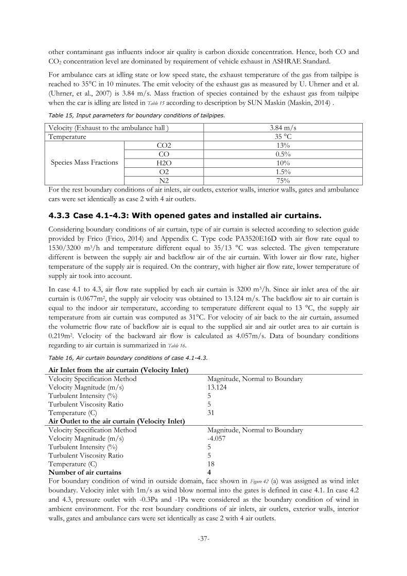
-37-

other contaminant gas influents indoor air quality is carbon dioxide concentration. Hence, both CO and

CO2 concentration level are dominated by requirement of vehicle exhaust in ASHRAE Standard.

For ambulance cars at idling state or low speed state, the exhaust temperature of the gas from tailpipe is

reached to 35°C in 10 minutes. The emit velocity of the exhaust gas as measured by U. Uhrner and et al.

(Uhrner, et al., 2007) is 3.84 m/s. Mass fraction of species contained by the exhaust gas from tailpipe

when the car is idling are listed in Table 15 according to description by SUN Maskin (Maskin, 2014) .

Table 15, Input parameters for boundary conditions of tailpipes.

Velocity (Exhaust to the ambulance hall ) 3.84 m/s

Temperature 35 °C

Species Mass Fractions

CO2 13%

CO 0.5%

H2O 10%

O2 1.5%

N2 75%

For the rest boundary conditions of air inlets, air outlets, exterior walls, interior walls, gates and ambulance

cars were set identically as case 2 with 4 air outlets.

4.3.3 Case 4.1-4.3: With opened gates and installed air curtains.

Considering boundary conditions of air curtain, type of air curtain is selected according to selection guide

provided by Frico (Frico, 2014) and Appendix C. Type code PA3520E16D with air flow rate equal to

1530/3200 m3/h and temperature different equal to 35/13 °C was selected. The given temperature

different is between the supply air and backflow air of the air curtain. With lower air flow rate, higher

temperature of the supply air is required. On the contrary, with higher air flow rate, lower temperature of

supply air took into account.

In case 4.1 to 4.3, air flow rate supplied by each air curtain is 3200 m3/h. Since air inlet area of the air

curtain is 0.0677m2, the supply air velocity was obtained to 13.124 m/s. The backflow air to air curtain is

equal to the indoor air temperature, according to temperature different equal to 13 °C, the supply air

temperature from air curtain was computed as 31°C. For velocity of air back to the air curtain, assumed

the volumetric flow rate of backflow air is equal to the supplied air and air outlet area to air curtain is

0.219m2. Velocity of the backward air flow is calculated as 4.057m/s. Data of boundary conditions

regarding to air curtain is summarized in Table 16.

Table 16, Air curtain boundary conditions of case 4.1-4.3.

Air Inlet from the air curtain (Velocity Inlet)

Velocity Specification Method Magnitude, Normal to Boundary Velocity Magnitude (m/s) 13.124 Turbulent Intensity (%) 5 Turbulent Viscosity Ratio 5 Temperature (C) 31 Air Outlet to the air curtain (Velocity Inlet)

Velocity Specification Method Magnitude, Normal to Boundary Velocity Magnitude (m/s) -4.057 Turbulent Intensity (%) 5 Turbulent Viscosity Ratio 5 Temperature (C) 18 Number of air curtains 4 For boundary condition of wind in outside domain, face shown in Figure 42 (a) was assigned as wind inlet

boundary. Velocity inlet with 1m/s as wind blow normal into the gates is defined in case 4.1. In case 4.2

and 4.3, pressure outlet with -0.3Pa and -1Pa were considered as the boundary condition of wind in

ambient environment. For the rest boundary conditions of air inlets, air outlets, exterior walls, interior

walls, gates and ambulance cars were set identically as case 2 with 4 air outlets.

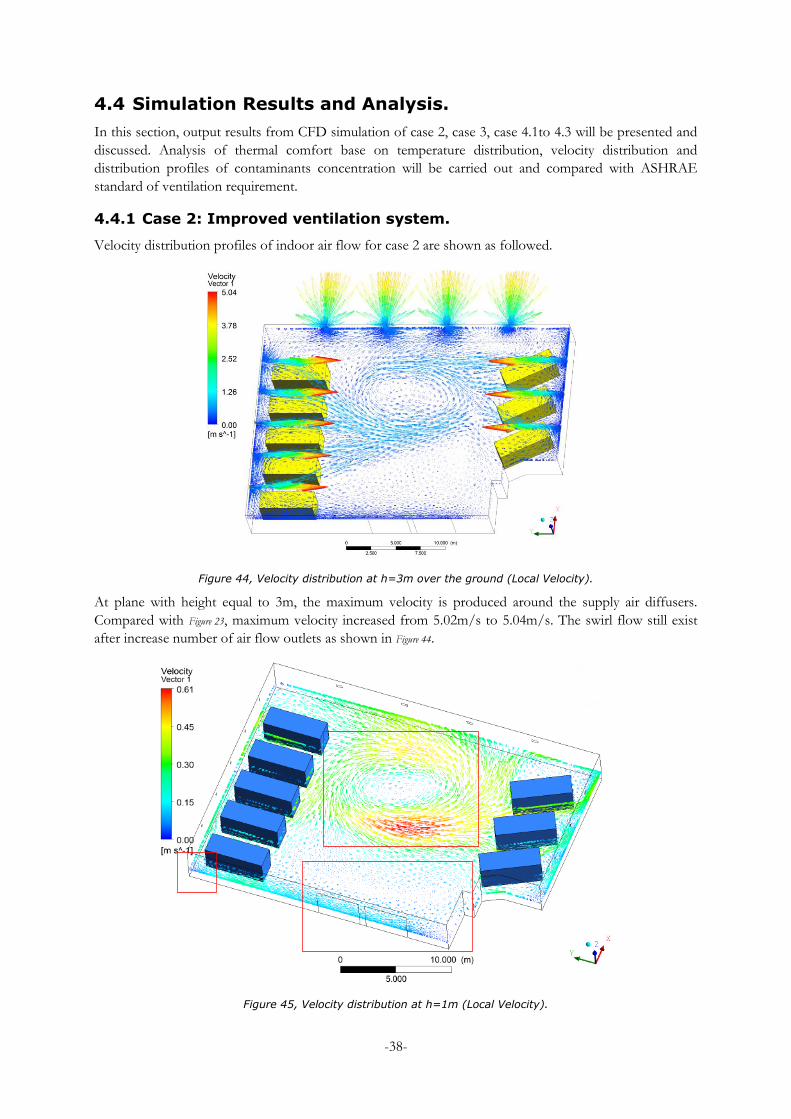
-38-

4.4 Simulation Results and Analysis.

In this section, output results from CFD simulation of case 2, case 3, case 4.1to 4.3 will be presented and

discussed. Analysis of thermal comfort base on temperature distribution, velocity distribution and

distribution profiles of contaminants concentration will be carried out and compared with ASHRAE

standard of ventilation requirement.

4.4.1 Case 2: Improved ventilation system.

Velocity distribution profiles of indoor air flow for case 2 are shown as followed.

Figure 44, Velocity distribution at h=3m over the ground (Local Velocity).

At plane with height equal to 3m, the maximum velocity is produced around the supply air diffusers.

Compared with Figure 23, maximum velocity increased from 5.02m/s to 5.04m/s. The swirl flow still exist

after increase number of air flow outlets as shown in Figure 44.

Figure 45, Velocity distribution at h=1m (Local Velocity).

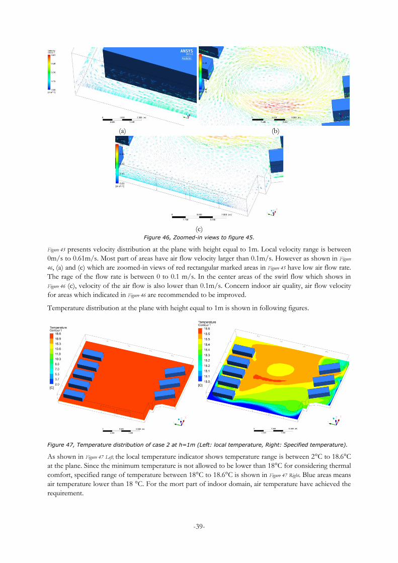
-39-

(a) (b)

(c)

Figure 46, Zoomed-in views to figure 45.

Figure 45 presents velocity distribution at the plane with height equal to 1m. Local velocity range is between

0m/s to 0.61m/s. Most part of areas have air flow velocity larger than 0.1m/s. However as shown in Figure

46, (a) and (c) which are zoomed-in views of red rectangular marked areas in Figure 45 have low air flow rate.

The rage of the flow rate is between 0 to 0.1 m/s. In the center areas of the swirl flow which shows in

Figure 46 (c), velocity of the air flow is also lower than 0.1m/s. Concern indoor air quality, air flow velocity

for areas which indicated in Figure 46 are recommended to be improved.

Temperature distribution at the plane with height equal to 1m is shown in following figures.

Figure 47, Temperature distribution of case 2 at h=1m (Left: local temperature, Right: Specified temperature).

As shown in Figure 47 Left, the local temperature indicator shows temperature range is between 2°C to 18.6°C

at the plane. Since the minimum temperature is not allowed to be lower than 18°C for considering thermal

comfort, specified range of temperature between 18°C to 18.6°C is shown in Figure 47 Right. Blue areas means

air temperature lower than 18 °C. For the mort part of indoor domain, air temperature have achieved the

requirement.

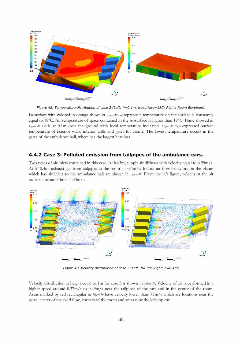
-40-

Figure 48, Temperature distribution of case 2 (Left: h=0.1m, isosurface=18C; Right: Room Envelope).

Isosurface with colored in orange shows in Figure 48 Left represents temperature on the surface is constantly

equal to 18°C. Air temperature of space contained in the isosurface is higher than 18°C. Plane showed in

Figure 48 Left is at 0.1m over the ground with local temperature indicated. Figure 48 Right expressed surface

temperature of exterior walls, interior walls and gates for case 2. The lowest temperature occurs in the

gates of the ambulance hall, where has the largest heat loss.

4.4.2 Case 3: Polluted emission from tailpipes of the ambulance cars.

Two types of air inlets contained in this case. At h=3m, supply air diffuser with velocity equal to 4.99m/s.

At h=0.4m, exhaust gas from tailpipes to the room is 3.84m/s. Indoor air flow behaviors on the planes

which has air inlets to the ambulance hall are shown in Figure 49. From the left figure, velocity at the air

outlets is around 3m/s-4.33m/s.

Figure 49, Velocity distribution of case 3 (Left: h=3m; Right: h=0.4m)

Velocity distribution at height equal to 1m for case 3 is shown in Figure 50. Velocity of air is performed in a

higher speed around 0.37m/s to 0.49m/s near the tailpipes of the cars and in the center of the room.

Areas marked by red rectangular in Figure 50 have velocity lower than 0.1m/s which are locations near the

gates, center of the swirl flow, corners of the room and areas near the left-top car.

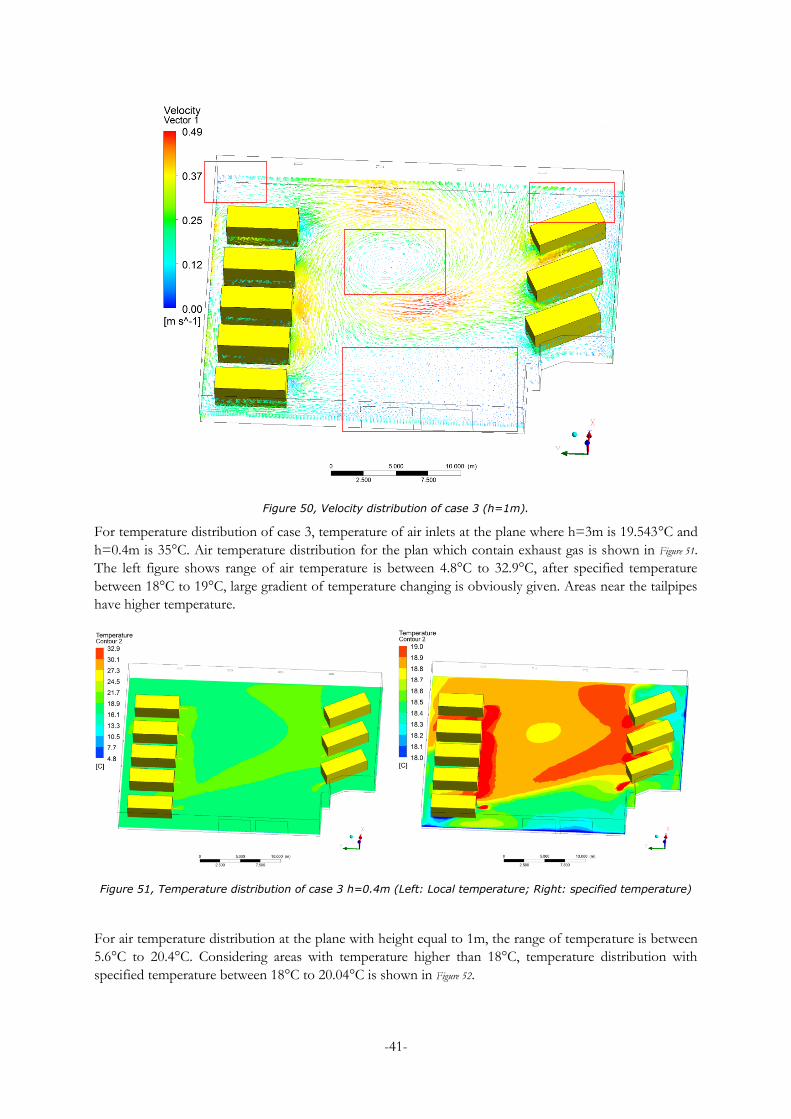
-41-

Figure 50, Velocity distribution of case 3 (h=1m).

For temperature distribution of case 3, temperature of air inlets at the plane where h=3m is 19.543°C and

h=0.4m is 35°C. Air temperature distribution for the plan which contain exhaust gas is shown in Figure 51.

The left figure shows range of air temperature is between 4.8°C to 32.9°C, after specified temperature

between 18°C to 19°C, large gradient of temperature changing is obviously given. Areas near the tailpipes

have higher temperature.

Figure 51, Temperature distribution of case 3 h=0.4m (Left: Local temperature; Right: specified temperature)

For air temperature distribution at the plane with height equal to 1m, the range of temperature is between

5.6°C to 20.4°C. Considering areas with temperature higher than 18°C, temperature distribution with

specified temperature between 18°C to 20.04°C is shown in Figure 52.

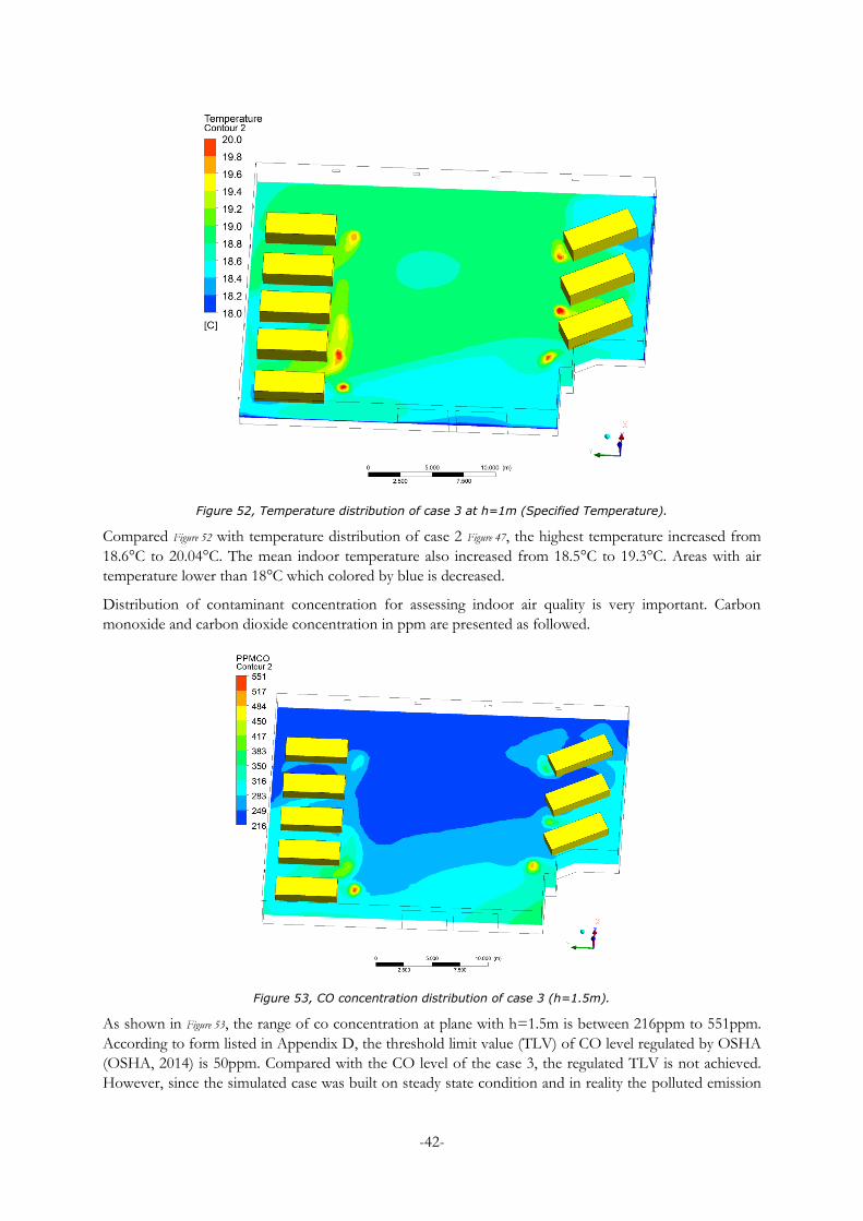
-42-

Figure 52, Temperature distribution of case 3 at h=1m (Specified Temperature).

Compared Figure 52 with temperature distribution of case 2 Figure 47, the highest temperature increased from

18.6°C to 20.04°C. The mean indoor temperature also increased from 18.5°C to 19.3°C. Areas with air

temperature lower than 18°C which colored by blue is decreased.

Distribution of contaminant concentration for assessing indoor air quality is very important. Carbon

monoxide and carbon dioxide concentration in ppm are presented as followed.

Figure 53, CO concentration distribution of case 3 (h=1.5m).

As shown in Figure 53, the range of co concentration at plane with h=1.5m is between 216ppm to 551ppm.

According to form listed in Appendix D, the threshold limit value (TLV) of CO level regulated by OSHA

(OSHA, 2014) is 50ppm. Compared with the CO level of the case 3, the regulated TLV is not achieved.

However, since the simulated case was built on steady state condition and in reality the polluted emission

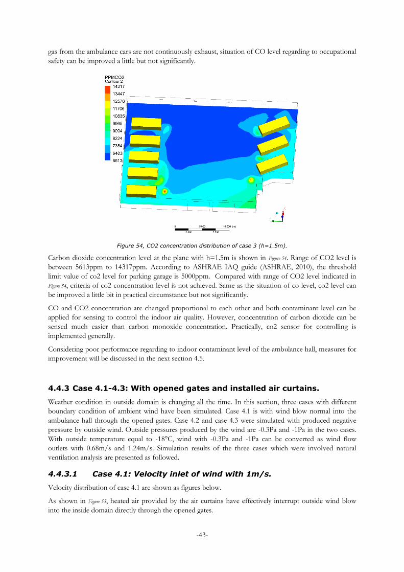
-43-

gas from the ambulance cars are not continuously exhaust, situation of CO level regarding to occupational

safety can be improved a little but not significantly.

Figure 54, CO2 concentration distribution of case 3 (h=1.5m).

Carbon dioxide concentration level at the plane with h=1.5m is shown in Figure 54. Range of CO2 level is

between 5613ppm to 14317ppm. According to ASHRAE IAQ guide (ASHRAE, 2010), the threshold

limit value of co2 level for parking garage is 5000ppm. Compared with range of CO2 level indicated in

Figure 54, criteria of co2 concentration level is not achieved. Same as the situation of co level, co2 level can

be improved a little bit in practical circumstance but not significantly.

CO and CO2 concentration are changed proportional to each other and both contaminant level can be

applied for sensing to control the indoor air quality. However, concentration of carbon dioxide can be

sensed much easier than carbon monoxide concentration. Practically, co2 sensor for controlling is

implemented generally.

Considering poor performance regarding to indoor contaminant level of the ambulance hall, measures for

improvement will be discussed in the next section 4.5.

4.4.3 Case 4.1-4.3: With opened gates and installed air curtains.

Weather condition in outside domain is changing all the time. In this section, three cases with different

boundary condition of ambient wind have been simulated. Case 4.1 is with wind blow normal into the

ambulance hall through the opened gates. Case 4.2 and case 4.3 were simulated with produced negative

pressure by outside wind. Outside pressures produced by the wind are -0.3Pa and -1Pa in the two cases.

With outside temperature equal to -18°C, wind with -0.3Pa and -1Pa can be converted as wind flow

outlets with 0.68m/s and 1.24m/s. Simulation results of the three cases which were involved natural

ventilation analysis are presented as followed.

4.4.3.1 Case 4.1: Velocity inlet of wind with 1m/s.

Velocity distribution of case 4.1 are shown as figures below.

As shown in Figure 55, heated air provided by the air curtains have effectively interrupt outside wind blow

into the inside domain directly through the opened gates.

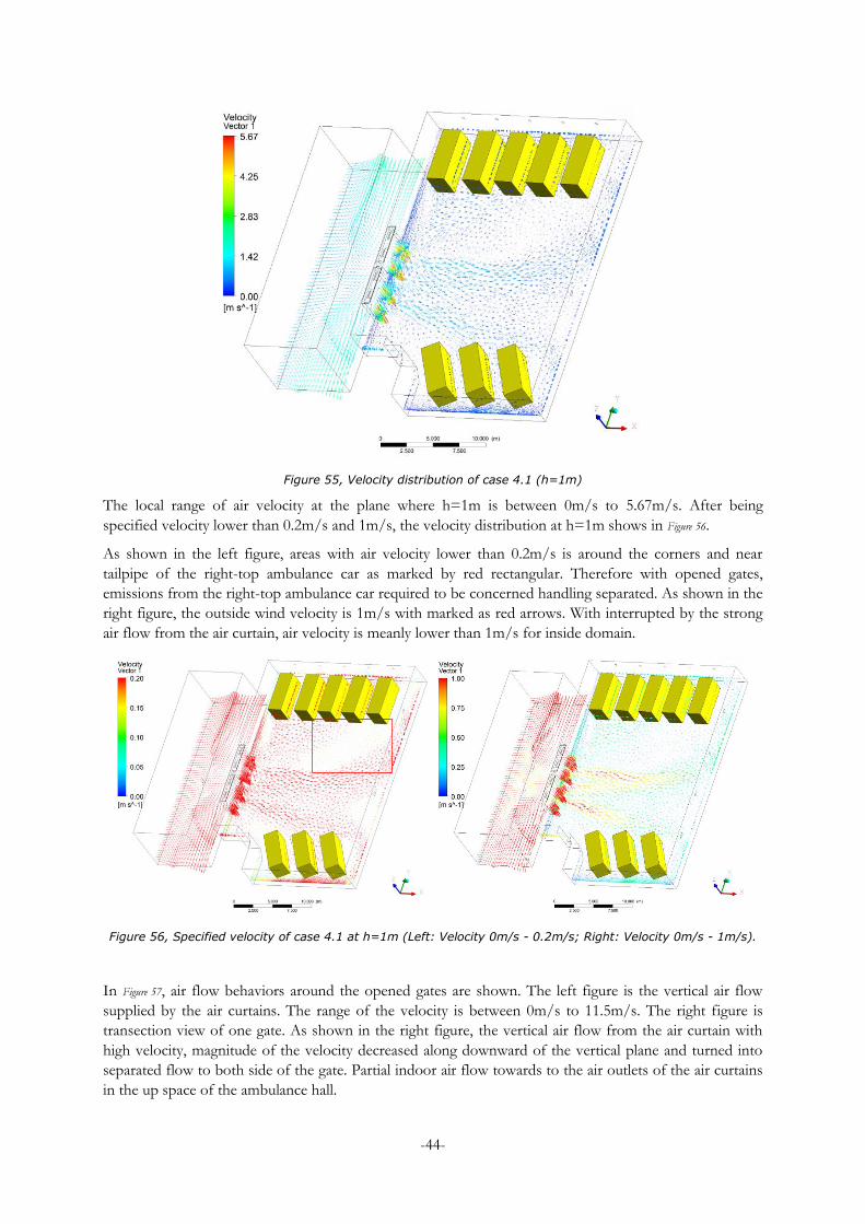
-44-

Figure 55, Velocity distribution of case 4.1 (h=1m)

The local range of air velocity at the plane where h=1m is between 0m/s to 5.67m/s. After being

specified velocity lower than 0.2m/s and 1m/s, the velocity distribution at h=1m shows in Figure 56.

As shown in the left figure, areas with air velocity lower than 0.2m/s is around the corners and near

tailpipe of the right-top ambulance car as marked by red rectangular. Therefore with opened gates,

emissions from the right-top ambulance car required to be concerned handling separated. As shown in the

right figure, the outside wind velocity is 1m/s with marked as red arrows. With interrupted by the strong

air flow from the air curtain, air velocity is meanly lower than 1m/s for inside domain.

Figure 56, Specified velocity of case 4.1 at h=1m (Left: Velocity 0m/s - 0.2m/s; Right: Velocity 0m/s - 1m/s).

In Figure 57, air flow behaviors around the opened gates are shown. The left figure is the vertical air flow

supplied by the air curtains. The range of the velocity is between 0m/s to 11.5m/s. The right figure is

transection view of one gate. As shown in the right figure, the vertical air flow from the air curtain with

high velocity, magnitude of the velocity decreased along downward of the vertical plane and turned into

separated flow to both side of the gate. Partial indoor air flow towards to the air outlets of the air curtains

in the up space of the ambulance hall.

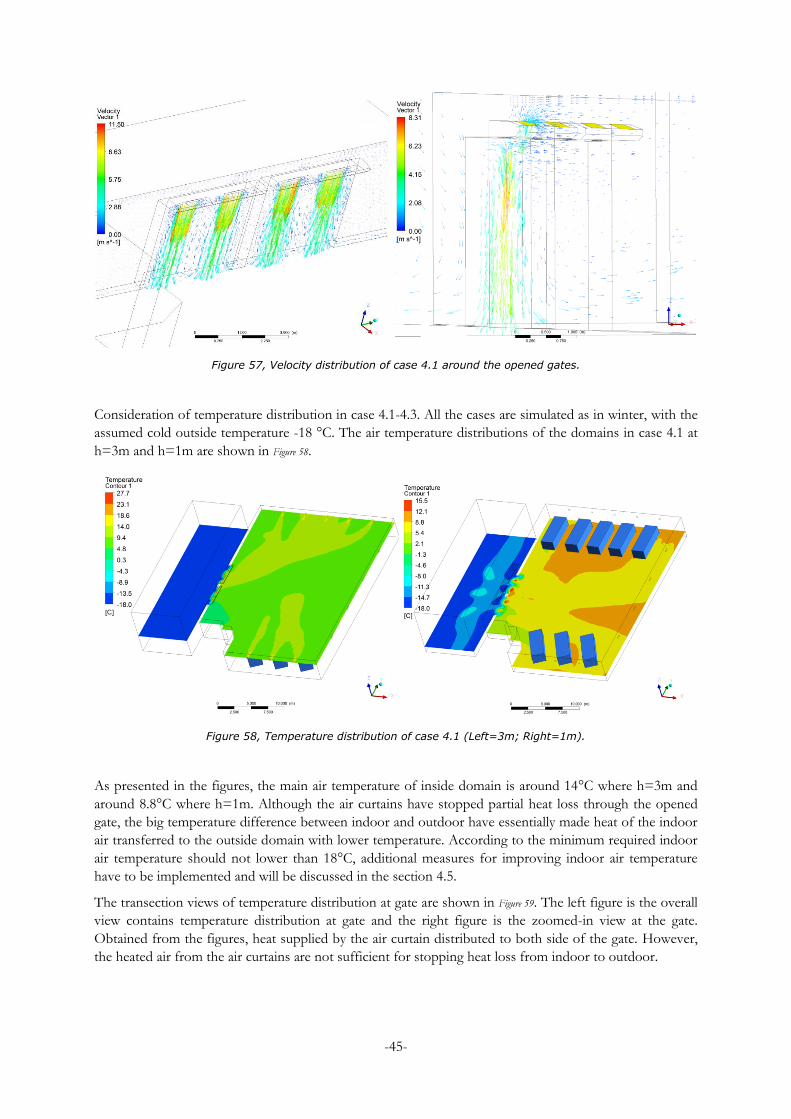
-45-

Figure 57, Velocity distribution of case 4.1 around the opened gates.

Consideration of temperature distribution in case 4.1-4.3. All the cases are simulated as in winter, with the

assumed cold outside temperature -18 °C. The air temperature distributions of the domains in case 4.1 at

h=3m and h=1m are shown in Figure 58.

Figure 58, Temperature distribution of case 4.1 (Left=3m; Right=1m).

As presented in the figures, the main air temperature of inside domain is around 14°C where h=3m and

around 8.8°C where h=1m. Although the air curtains have stopped partial heat loss through the opened

gate, the big temperature difference between indoor and outdoor have essentially made heat of the indoor

air transferred to the outside domain with lower temperature. According to the minimum required indoor

air temperature should not lower than 18°C, additional measures for improving indoor air temperature

have to be implemented and will be discussed in the section 4.5.

The transection views of temperature distribution at gate are shown in Figure 59. The left figure is the overall

view contains temperature distribution at gate and the right figure is the zoomed-in view at the gate.

Obtained from the figures, heat supplied by the air curtain distributed to both side of the gate. However,

the heated air from the air curtains are not sufficient for stopping heat loss from indoor to outdoor.

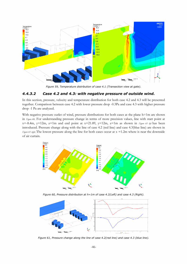
-46-

Figure 59, Temperature distribution of case 4.1 (Transection view at gate).

4.4.3.2 Case 4.2 and 4.3: with negative pressure of outside wind.

In this section, pressure, velocity and temperature distribution for both case 4.2 and 4.3 will be presented

together. Comparison between case 4.2 with lower pressure drop -0.3Pa and case 4.3 with higher pressure

drop -1 Pa are analyzed.

With negative pressure outlet of wind, pressure distributions for both cases at the plane h=1m are shown

in Figure 60. For understanding pressure change in terms of more precision values, line with start point at

x=-8.4m, y=12m, z=1m and end point at x=21.89, y=12m, z=1m as shown in Figure 61 left has been

introduced. Pressure change along with the line of case 4.2 (red line) and case 4.3(blue line) are shown in

Figure 61 right. The lowest pressure along the line for both cases occur at x =1.2m where is near the downside

of air curtain.

Figure 60, Pressure distribution at h=1m of case 4.2(Left) and case 4.3 (Right).

Figure 61, Pressure change along the line of case 4.2(red line) and case 4.3 (blue line).

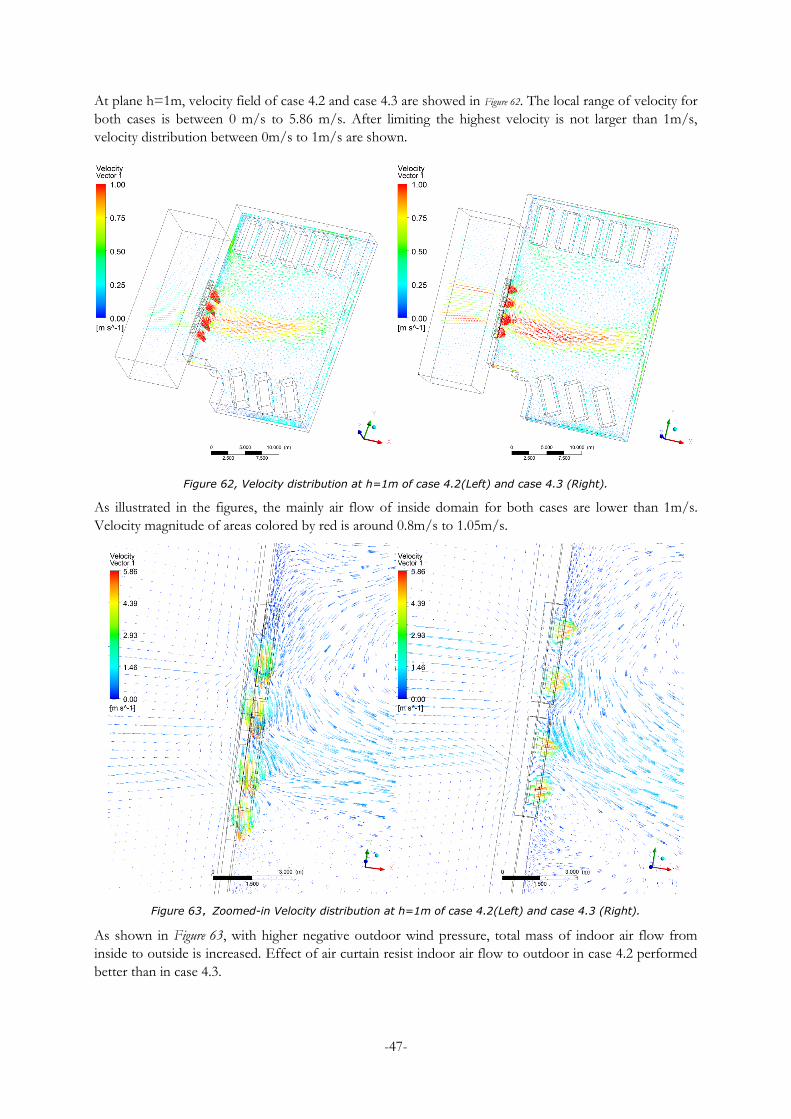
-47-

At plane h=1m, velocity field of case 4.2 and case 4.3 are showed in Figure 62. The local range of velocity for

both cases is between 0 m/s to 5.86 m/s. After limiting the highest velocity is not larger than 1m/s,

velocity distribution between 0m/s to 1m/s are shown.

Figure 62, Velocity distribution at h=1m of case 4.2(Left) and case 4.3 (Right).

As illustrated in the figures, the mainly air flow of inside domain for both cases are lower than 1m/s.

Velocity magnitude of areas colored by red is around 0.8m/s to 1.05m/s.

Figure 63，Zoomed-in Velocity distribution at h=1m of case 4.2(Left) and case 4.3 (Right).

As shown in Figure 63, with higher negative outdoor wind pressure, total mass of indoor air flow from

inside to outside is increased. Effect of air curtain resist indoor air flow to outdoor in case 4.2 performed

better than in case 4.3.

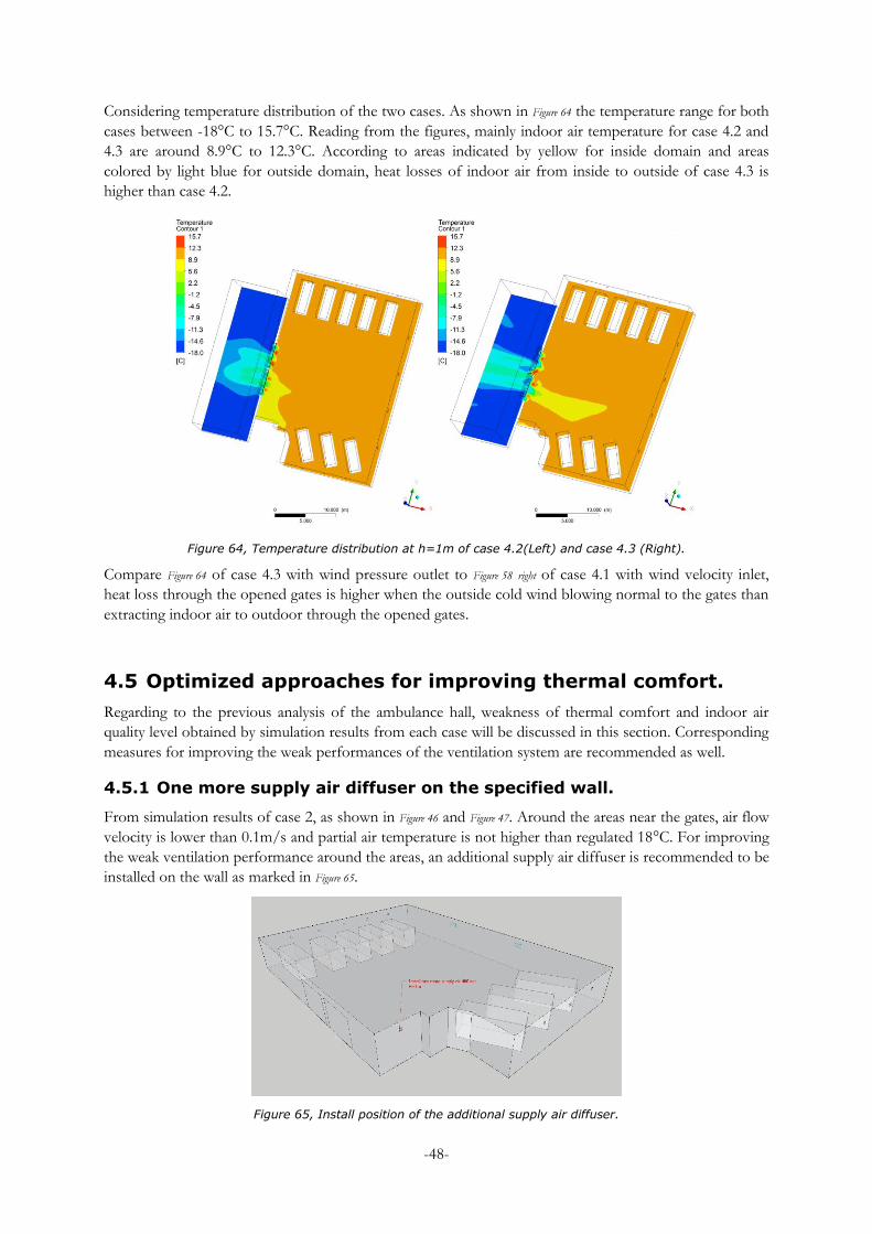
-48-

Considering temperature distribution of the two cases. As shown in Figure 64 the temperature range for both

cases between -18°C to 15.7°C. Reading from the figures, mainly indoor air temperature for case 4.2 and

4.3 are around 8.9°C to 12.3°C. According to areas indicated by yellow for inside domain and areas

colored by light blue for outside domain, heat losses of indoor air from inside to outside of case 4.3 is

higher than case 4.2.

Figure 64, Temperature distribution at h=1m of case 4.2(Left) and case 4.3 (Right).

Compare Figure 64 of case 4.3 with wind pressure outlet to Figure 58 right of case 4.1 with wind velocity inlet,

heat loss through the opened gates is higher when the outside cold wind blowing normal to the gates than

extracting indoor air to outdoor through the opened gates.

4.5 Optimized approaches for improving thermal comfort.

Regarding to the previous analysis of the ambulance hall, weakness of thermal comfort and indoor air

quality level obtained by simulation results from each case will be discussed in this section. Corresponding

measures for improving the weak performances of the ventilation system are recommended as well.

4.5.1 One more supply air diffuser on the specified wall.

From simulation results of case 2, as shown in Figure 46 and Figure 47. Around the areas near the gates, air flow

velocity is lower than 0.1m/s and partial air temperature is not higher than regulated 18°C. For improving

the weak ventilation performance around the areas, an additional supply air diffuser is recommended to be

installed on the wall as marked in Figure 65.

Figure 65, Install position of the additional supply air diffuser.

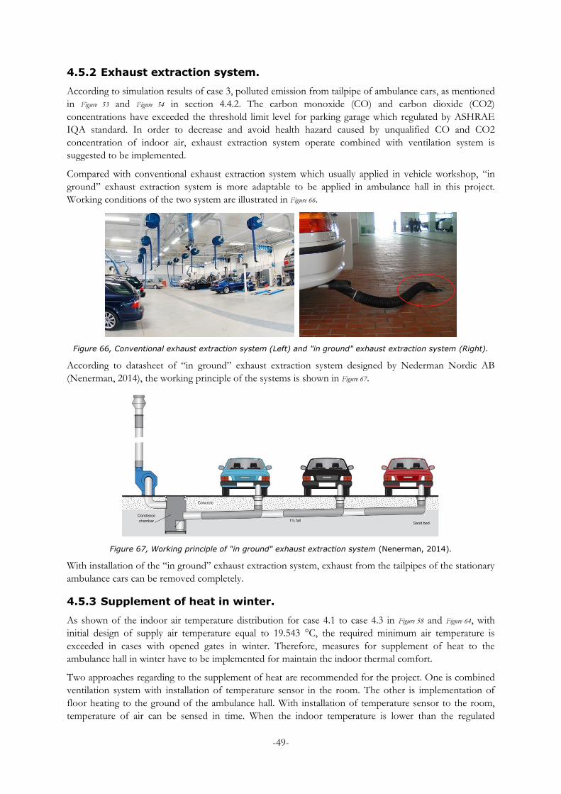
-49-

4.5.2 Exhaust extraction system.

According to simulation results of case 3, polluted emission from tailpipe of ambulance cars, as mentioned

in Figure 53 and Figure 54 in section 4.4.2. The carbon monoxide (CO) and carbon dioxide (CO2)

concentrations have exceeded the threshold limit level for parking garage which regulated by ASHRAE

IQA standard. In order to decrease and avoid health hazard caused by unqualified CO and CO2

concentration of indoor air, exhaust extraction system operate combined with ventilation system is

suggested to be implemented.

Compared with conventional exhaust extraction system which usually applied in vehicle workshop, “in

ground” exhaust extraction system is more adaptable to be applied in ambulance hall in this project.

Working conditions of the two system are illustrated in Figure 66.

Figure 66, Conventional exhaust extraction system (Left) and "in ground" exhaust extraction system (Right).

According to datasheet of “in ground” exhaust extraction system designed by Nederman Nordic AB

(Nenerman, 2014), the working principle of the systems is shown in Figure 67.

Figure 67, Working principle of "in ground" exhaust extraction system (Nenerman, 2014).

With installation of the “in ground” exhaust extraction system, exhaust from the tailpipes of the stationary

ambulance cars can be removed completely.

4.5.3 Supplement of heat in winter.

As shown of the indoor air temperature distribution for case 4.1 to case 4.3 in Figure 58 and Figure 64, with

initial design of supply air temperature equal to 19.543 °C, the required minimum air temperature is

exceeded in cases with opened gates in winter. Therefore, measures for supplement of heat to the

ambulance hall in winter have to be implemented for maintain the indoor thermal comfort.

Two approaches regarding to the supplement of heat are recommended for the project. One is combined

ventilation system with installation of temperature sensor in the room. The other is implementation of

floor heating to the ground of the ambulance hall. With installation of temperature sensor to the room,

temperature of air can be sensed in time. When the indoor temperature is lower than the regulated

-50-

minimum temperature 18°C, signal obtained from the sensor induced increasing of supply air

temperature. Compared with conventional heating method as installation of radiators, floor heating

combined with recovery of waste heat which collected from the exhaust of stationary ambulance cars is a

more energy efficient approach.

-51-

5 Conclusion and future improvement

The objective of this master thesis is to build numerical simulation of an ambulance hall for assessing

indoor fluid flied and thermal comfort. The main contents of the thesis are divided into two main parts.

The first part is to make comparison between the three CFD software which are ANSYS Fluent, Star-

CCM+ and IESVE Microflo. The second part is CFD modeling of the ambulance hall by ANSYS Fluent

with different boundary conditions.

In the first part, after simulated the baseline model by the three software, the presented results from each

cases shows that all the selected CFD software are qualitatively to compute convection diffusion problems.

However, IESVE Microflo performs less precision, lower correctness and more time cost for CFD

modeling compared with ANSYS Fluent and Star-CCM+. In contrast to case 1.2 and 1.3, case 1.1 with

CFD modeling by ANSYS Fluent have saved simulating time with accurate and efficient simulation

processing. In summary, for analyzing complicated indoor fluid environment by numerical simulation,

ANSYS Fluent is recommended for its’ best performance.

In the second part, five types of boundary conditions for three cases have been implemented. Simulation

results of case 2 and case 3 have shown the designed ventilation system for the ambulance hall satisfied

thermal comfort level which regulated by ASHRAE standard with closed gates. Nevertheless, threshold

limit value of the contaminants concentration which regulated by ASHRAE IAQ Standard cannot be

achieved. From simulation results of case 4.1 to 4.3 shown that the designed ventilation system cannot

satisfy indoor thermal comfort level when the gates of the ambulance hall opened in winter. In conclusion,

measures for decreasing contaminants concentration and increasing indoor air temperature demanded to

be considered in further design and three recommended measures for optimizing the design introduced in

the end as a reference.

-52-

6 Bibliography

ASHRAE, 1997. ASHRAE Handbook. Fundamentals Volume ed. GA: ASHRAE.

ASHRAE, 2010. ASHRAE Indoor Air Quality Guide.. U.S.: ASHRAE.

Barth, T. J. & Jesperson, D. C., 1989. The design and application of upwind schemes on unstructured meshes, Reno:

AIAA.

Calautit, J. K., Hughes, B. R. & Ghani, S. A., 2012. A numerical investigation into the feasibility of integrating green

building technologies into row houses in the Middle East, London: Taylor & Francis.

CD-adapco, 2013. Star-CCM+ User Guide. [Online]

Available at: file:///C:/Program%20Files/CD-adapco/STAR-CCM+9.02.005-

R8/doc/online/index.htm#page/STARCCMP/navigatingHelp.001.1.html

Cehlin, M., 2006. Visualization of Airflow, Temperature and Concentration Indoors Whole-field measuring methods and

CFD , Stockholm: Centre of Built Environment, KTH.

Cho, H. K., Lee, H. D., Park, . I. . K. & Jeong, J. J., 2010. Implementation of a second-order upwind method in a

semi-implicit two-phase flow code on unstructured meshes., Republic of Korea: ELSEVIER.

Crippa, S., 2011. Improvement of Unstructured Computational Fluid Dynamics Simulations Through Novel Mesh

Generation Methodologies, Braunschweig: JOURNAL OFAIRCRAFT.

Eleni, D. C., Athanasios, T. I. & Dionissios, M. P., 2012. Evaluation of the turbulence models for the

simulation of the flow over a National Advisory Committee for Aeronautics (NACA) 0012 airfoil. Journal

of Mechanical Engineering Research , 4(3)(2141-2383), pp. 100-111.

Fluent, A., 2006. ANSYS Fluent User Guide. [Online]

Available at: http://aerojet.engr.ucdavis.edu/fluenthelp/html/ug/node155.htm

[Accessed 20 09 2006].

Frico, 2014. Air curtain selection guide.. [Online]

Available at: http://www.frico.se/en/products/Air-curtain-selection/

Hach, L. & Katoh , Y., 2010. THE AIR CHANGE RATE CONTROL BY LOCAL MEAN AGE OF

AIR IN VENTILATED SPACES., Prague: Institute of Chemical Technology.

Hirsch, C., 2007. Numerical Computation of Internal and External Flows - Fundamentals of Computational Fluid

Dynamics. (2nd Edition) ed. India: Elsevier.

ISO, 1994. ISO 7730 : 1994 Ergonomics of the thermal environment -- Analytical determination and interpretation of

thermal comfort using calculation of the PMV and PPD indices and local thermal comfort criteria, Switzerland:

International Organization for Standardization.

Launder, B. E. & Spalding, D. B., 1973. THE NUMERICAL COMPUTATION OF TURBULENT

FLOWS, London: North-Holland Publishing Company.

Markatos , C. N., 2004. The mathematical modelling of turbulent flows, London: Centre for Numerical Modelling

and Process Analysis.

Maskin, S., 2014. SUN Avgasskola. [Online]

Available at: http://sunmaskin.se/utbildningar/sun-avgasskola

McQuiston, F. C., Parker, J. D. & Spitler, J. D., 2005. Heat, ventilating, and air conditioning (Anlysis and

Design).. Sixth Edition ed. U.S.: WILEY.

Nenerman, 2014. In Ground Exhaust Extraction System for stationary vehicles.. [Online]

Available at: http://www.nederman.com/products/exhaust-extraction/vehicle-exhaust-

extraction/~/media/ExtranetDocuments/PublishedTechnicalLeaflet/150390_00__In_Ground.ashx

-53-

OSHA, 2014. Occupational Safety & Health Administration of U.S. Department of Labor.. [Online]

Available at: https://www.osha.gov/

Shih, T.-H.et al., 1994. A new k-ε eddy viscosity model for high reynolds number turbulent flows, U.S.A: Elsevier.

Stamou, A., Katsiris, I. & Schaelin, A., 2007. Evaluation of thermal comfort in Galatsi Arena of the Olympics

‘‘Athens 2004’’ using a CFD model, Switzerland: ScienceDirect.

Tyler, H. et al., 2013. CBE Thermal Comfort Tool. [Online]

Available at: http://cbe.berkeley.edu/comforttool/

Uhrner, U. et al., 2007. Dilution and aerosol dynamics within a diesel car exhaust plume—CFD simulations of on-road

measurement conditions., Germany: ELSEVIER.

Versteeg, H. K. & Malalasekera, W., 2007. A introduction to computional fluid dynamics - The finite volume method.

Second edition ed. London: PEARSON.

Xue, H. & Ho, J. C., 2000. Modelling of Heat and Carbon Monoxide Emitted from Moving Cars in an Underground

Car Park., Singapore: Elsevier.

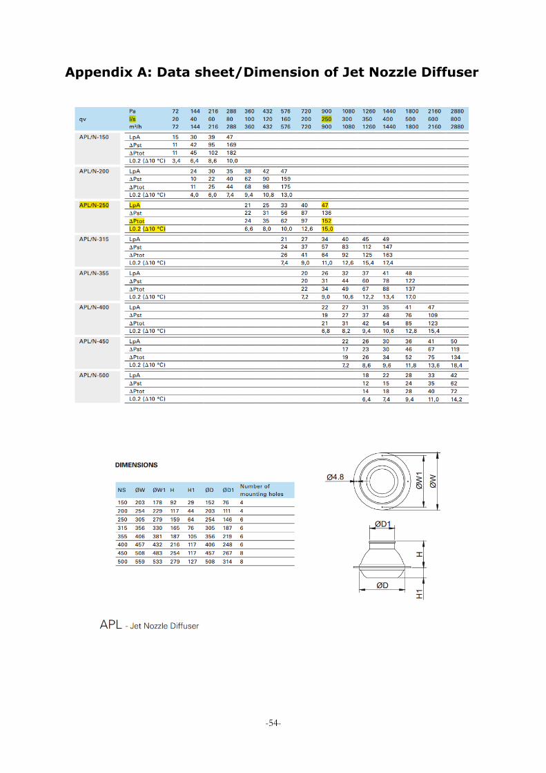
-54-

Appendix A: Data sheet/Dimension of Jet Nozzle Diffuser

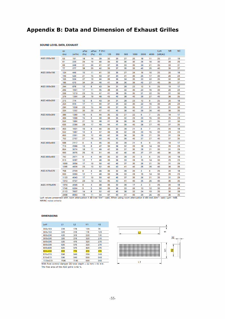
-55-

Appendix B: Data and Dimension of Exhaust Grilles

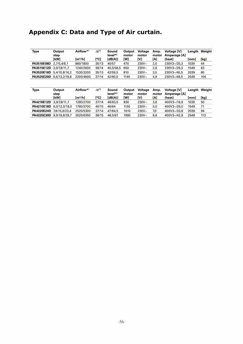
-56-

Appendix C: Data and Type of Air curtain.

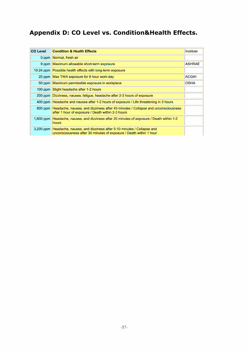
-57-

Appendix D: CO Level vs. Condition&Health Effects.