Embed Size (px)
Citation preview
ORIGINAL
Comparison of different kinetic models for the heat transferproblem
Irina A. Graur • A. P. Polikarpov
Received: 26 June 2009 / Accepted: 30 October 2009 / Published online: 20 November 2009
� Springer-Verlag 2009
Abstract The steady-state heat transfer problem between
two parallel plates is investigated using kinetic models of
the Boltzmann equation: BGK, S-model and ES-model. The
discrete velocity method is used to determine the values of
physical parameters: density, bulk velocity, temperature
and heat flux. The obtained results are compared with the
analytical expressions and some experimental data.
List of symbols
t Time
f One particle distribution function
r = (x,y,z) Position vector
v Molecular velocity
u Bulk velocity
V = v - u Peculiar velocity
vm The most probable molecular speed
c Dimensionless molecular velocity
n Number density
T Temperature
q Heat flux vector
Pij Stress tensor
p Gas pressure
m Molecular mass of the gas
k Boltzmann constant
Pr Prandtl number
H Distance between the plates
Greek symbols
a Accommodation coefficient
d Rarefaction parameter
DT Temperature difference between the plates
s Relaxation time
U, W Reduced distribution functions
l Shear viscosity
Subscript
0 Values on the symmetry axis (y = 0)
w Wall quantities
FM Free molecular quantities
Superscript
mod Model distribution function
M Maxwellian distribution function
± Parameters of reflected/incident molecules
1 Introduction
A systematic research effort in micro mechanics devices
started in the late 1980s. Microducts, micronozzles,
micropumps, microturbines and microvalves are examples
of small devices involving liquid and gas flows. The
characteristic length scale of these devices is less than
1 mm but more than 1 micron. Therefore, even at atmo-
spheric conditions, the mean-free path to characteristic
dimension ratio cannot be neglected and so in the flow
dynamic associated with microelectromechanical systems
(MEMS) rarefied gas phenomena become apparent.
The correct description of the rarefied gas flows for the
complete Knudsen number range is based on the Boltzmann
kinetic equation. The difficulties associated with its resolu-
tion come from the large number of the independent vari-
ables (seven in the non stationary case), but also from a very
complicated structure of the collision integral. Therefore, in
the late sixties, several models of kinetic equations were
suggested (BGK, ES, S models), where the collision integral
I. A. Graur (&) � A. P. Polikarpov
Universite de Provence, Ecole Polytechnique Universitaire de
Marseille, UMR CNRS 6595, 5 rue Enrico Fermi,
13453 Marseille, France
e-mail: [email protected]
123
Heat Mass Transfer (2009) 46:237–244
DOI 10.1007/s00231-009-0558-x
is replaced by a relaxation term, which preserves various
important properties of the Boltzmann collision integral.
The main aim of the present paper is a test of validity
and of applicability of three kinetic models to describe
correctly the heat flux in the transitional flow regime. The
classical problem of a gas confined between two heated
plates is chosen as test case. This problem has been studied
by many authors, but especially using the linearized for-
mulation of the full Boltzmann or kinetic model equations
[3, 15, 17, 19]. But some of them have also solved the non-
linearized kinetic equations [12, 13]. In the present analysis
the numerical solutions of the heat transfer problem
between two parallel plates are obtained using three non-
linear model kinetic equations: BGK, S, ES models in the
transitional flow regime. These solutions are compared
with the numerical solution of the full Boltzmann equation
associated to the hard sphere model [12], with the DSMC
results [22] and with the experimental data [1, 18]. In
addition for the free molecular regime the numerical results
are compared with an analytical solution [10].
2 Kinetic models
To obtain the flow parameters in the transition regime the
Boltzmann equation should be solved:
of
otþ v � of
or¼ Qðf ; f 0Þ; ð1Þ
where t is the time, f(t, r, v) is the one particle distribution
function, r is the position vector, v is the molecular
velocity, Q(f, f0) is the collision integral. This equation
provides reliable numerical data but requires great
computational efforts. To reduce these efforts the
collision integral may be simplified and replaced by a
relaxation term, remaining its main properties:
of
otþ v � of
or¼ Iðf ; f modÞ; ð2Þ
where I (f, fmod) is the model collision integral
Iðf ; f modÞ ¼ f mod � f
s; ð3Þ
fmod, so called model distribution function, is an equilib-
rium distribution function which depends on the kinetic
model, s is a relaxation time. Different kinetic models were
proposed in the last sixties: BGK [4], S-model [14] and
ellipsoidal model (ES-model) [9]. In the present paper we
apply all these kinetic models for the steady flow simula-
tion and in the next section we will give a brief description
of each one.
When the distribution function is known, the macro-
scopic parameters may be calculated from the following
expressions:
number density and bulk velocity
nðrÞ ¼Zþ1
�1
f ðr; vÞdv; uðrÞ ¼ 1
n
Zþ1
�1
vf ðr; vÞdv; ð4Þ
temperature and heat flow vector
TðrÞ ¼ m
3nk
Zþ1
�1
V2f ðr; vÞdv;
qðrÞ ¼ m
2
Zþ1
�1
VV2f ðr; vÞdv;
ð5Þ
stress tensor
PijðrÞ ¼ m
Zþ1
�1
ViVjf ðr; vÞdv; ð6Þ
where V = v - u(r) is the peculiar velocity.
2.1 BGK
For the BGK kinetic equation [4] the equilibrium distri-
bution function fmod is the local Maxwellian distribution:
f mod ¼ f Mðn; T ; uÞ
¼ nðrÞ m
2pkTðrÞ
� �3=2
exp �mðv� uðrÞÞ2
2kTðrÞ
" #; ð7Þ
n is the number density, u is the bulk velocity, m is
the molecular mass of the gas, T is the gas temperature, k is
the Boltzmann constant. According to the construction
of the model kinetic equation the first five moments of
exact collision integral Q(f, f0) coincide with the first five
moments of the model collision integralZwQðf ; f 0Þdv ¼
ZwIðf ; f modÞdv ¼ MðwÞ;
where w ¼ 1; v; v2; ð8Þ
where here M(w) = 0. These properties derive from the
conservation of particles, momentum and energy in every
collision. Consequently, Eq. 2 provides the same macro-
scopic conservation laws as the Boltzmann equation 1 itself.
In this model the relaxation time is assumed to be
independent of the molecular velocity. The following
expression
s ¼ lp; ð9Þ
where p is the gas pressure and l is the shear viscosity,
provides the convenient expression of l. Since using
expression (9) in Eq. 2 and applying the Chapman–Enskog
method respectively to Eqs. 1 and 2 one obtains the same
expression of the viscosity coefficient.
238 Heat Mass Transfer (2009) 46:237–244
123
A number of important properties of the Boltzmann
collision integral are shared by the BGK model [9],
notably:
– The collision term drives the distribution function
toward equilibrium and vanishes, if and only if, the
distribution function fmod is equal to the local
Maxwellian equilibrium function;
– the collision term conserves molecular mass, momen-
tum, and kinetic energy;
– the collision term is a v-functional of f(r, t, v), i.e., it
depends upon the values of f over the entire range of the
v-space but only considering the values taken at a
single point in (r, t) space;
– the collision term is invariant in form under rotation or
translation of coordinates.
The main shortcoming of this kinetic model is that the
Prandtl number is obtained equal to 1.
2.2 S-model
The author of [14] proposed a technique for constructing an
approximate kinetic equation which is based on an
approximation of the collision integral. For this approxi-
mate equation the first few moment equations coincide
with the exact moment equations. This approximate
equation, called Shakhov model kinetic equation, is a
generalization of the BGK model equation in the sense that
the approximation condition (8) is satisfied not only for 1,
v, v2, but also for viv2 momentum which is not equal to
zero. Consequently this model provides the correct Prandtl
number equal to 2/3 for monoatomic gases. For this model
the equilibrium distribution function is given as
f mod ¼ f Sðn; T ; uÞ
¼ f M 1þ 2m
15nðrÞðkTðrÞÞ2V � qðrÞ mV2
2kTðrÞ �5
2
� �" #;
ð10Þ
where the bulk velocity u and the heat flux vector q are
defined by (4), (5).
Since the expression for fS contains the third-order
polynomial of v the distribution function may become
negative in the region of the large values of the velocities,
where the distribution itself is small. The H theorem is not
proved, but the author [20] gives some comments about the
correctness of the H-theorem for the S-model.
2.3 ES model
Holway [9] proposed a model based on the requirement for
the model distribution function to have the same first five
moments as the distribution function solution of the model
kinetic equation. In addition, the maximal probability
principle is used to obtain this ellipsoidal model [9]. This
model retains much of the mathematical simplicity of the
BGK model, but also yields the correct Prandtl number for
a monoatomic gas. In this model the equilibrium distribu-
tion function is replaced by the generalized Gaussian in the
following form [9]:
f mod ¼ f ESðn; T; uÞ ¼ n
p3=2ffiffiffiffiffiffiffiffiffiffiffiffidet Aij
p exp �X3
i;j¼1
A�1ij ViVj
" #;
ð11Þ
here Aij is a tensor with components
Aij ¼2kT
m
1
Prdij �
2ð1� PrÞnmPr
Pij; ð12Þ
Aij-1 is the tensor inverse to Aij, dij is the Kronecker symbol,
the stress tensor Pij is given by (6). The relaxation time for
the ES-model is defined as follows
s ¼ lpPr
: ð13Þ
The H-theorem was proved recently in [2] for this model.
3 Application to the heat flux problem
3.1 Physical conditions and normalization
A gas is confined between two infinite parallel plates,
y = -H/2 and y = H/2, the plates are considered at dif-
ferent but constant temperatures T�w ¼ T0 � DT and
Tþw ¼ T0 þ DT . We supposed here that the flow is sta-
tionary and depends only on the y-coordinate, notably
because the plates are infinite and at constant temperatures.
We assume also the bulk velocity u and the heat flux vector
q to have only two components: u = (ux, uy, 0) and
q = (qx, qy, 0). For some flow conditions, which will be
noted separately, we consider also the case where the
higher plate is moving with a relative constant velocity
uw = (uw, 0, 0) in the x direction and the lower plate with
the same velocity in the opposite direction. Then in the
following we consider only the stationary case.
The gas rarefaction is characterized by the parameter d:
d ¼ Hp
lvm; vm ¼
ffiffiffiffiffiffiffiffi2kT
m
r; ð14Þ
where vm is the most probable molecular speed. Since the
viscosity is proportional to the molecular mean free path,
the rarefaction parameter d is inversely proportional to the
Knudsen number.
The following dimensionless quantities have been
introduced:
Heat Mass Transfer (2009) 46:237–244 239
123
�r ¼ r
H; �T ¼ T
T0
; v0 ¼ffiffiffiffiffiffiffiffiffiffi2kT0
m
r; c ¼ v
v0
; �n ¼ n
n0
;
�f ¼ fv3
0
n0
; �s ¼ sv0
H; �u ¼ u
v0
; �q ¼ 2
n0mv30
q;
Pij ¼Pij
p0
; �l ¼ ll0
: ð15Þ
The reference pressure p0 is equal to n0kT0, where index
0 means the flow conditions on the symmetry axis
(y = 0).
The reference value of the viscosity coefficient l0 at T0
is taken from [5]. The hard-sphere model is used here, so
the viscosity coefficient is equal to �l ¼ffiffiffiffi�T
p:
In the following we omit the bars over the dimensionless
variables.
3.2 Reduced equations
The dimensionless form of the model Eq. 2 in this spatially
one-dimensional and steady case is written as
cyof
oy¼ d0n
ffiffiffiffiTpðf mod � f Þ: ð16Þ
Equation 16 is one-dimensional in the physical space,
but the molecular velocity space has three independent
variables. However, it is possible to reduce the
computational costs, introducing the reduced distribution
function. Since we supposed that the bulk velocity and the
heat flux vector have only two components (the third
components along the z-direction are equal to 0), we can
eliminate easily the dependence of the distribution function
on the molecular velocity cz. Multiplying Eq. 16 by 1 and
by cz2, and integrating it with respect to cz we obtain two
reduced equations
cyoUoy¼ d0n
ffiffiffiffiTpðUmod � UÞ;
cyoWoy¼ d0n
ffiffiffiffiTpðWmod �WÞ; ð17Þ
where the reduced functions U and W are introduced in
order to eliminate the variable cz
Uðy; cx; cyÞ ¼Z
f ðy; cÞcz;
Wðy; cx; cyÞ ¼Z
f ðy; cÞc2z cz:
ð18Þ
In the BGK model frame the reduced model distribution
functions, obtained from Maxwellian function (7),
according to (18) have the form
Umod ¼ UM ¼ n
pTexp �ðc� uÞ2
T
" #;
Wmod ¼ WM ¼ 0:5TUM :
ð19Þ
In the S-model frame the reduced model distribution
functions, obtained from (10), have the form
Umod ¼ US ¼ UM 1þ 4
15
ðc� uÞqnT2
ðc� uÞ2
T� 2
! !;
Wmod ¼ WS ¼ WM 1þ 4
15
ðc� uÞqnT2
ðc� uÞ2
T� 1
! !:
ð20Þ
If the ES-model is used, the dimensionless form of the
tensor (10) reads
Aij ¼T
Prdij �
1� Pr
nPrPij: ð21Þ
The reduced model distribution functions are written as
Umod ¼ UES ¼ n
pffiffiffiap exp �
X2
i;j¼1
A�1ij ðci � uiÞðcj � ujÞ
" #;
Wmod ¼ WES ¼ 0:5A33UES; ð22Þ
where a = A11A22 - A12A21.
3.3 Kinetic boundary conditions
The solution of the model kinetic equation needs a
boundary condition for the distribution function f. Despite
considerable efforts to understand the process of energy
and momentum transfer between gas flow and the solid
surface, models for detailed gas-surface interaction mech-
anism are still lacking [21]. In this paper we will use the
Maxwell-type diffuse-specular boundary condition at the
wall. For the down plate it reads
fþð�H=2; cx; cy; czÞ¼ ð1� aÞf�ð�H=2; cx;�cy; czÞ þ afw; ð23Þ
where, f? and f- are the distribution functions of the
incident and reflected molecules respectively, fw is distri-
bution function of particles fully accommodated with the
wall, fw ¼ f Mw ¼ nw
pT�wexp½�ðc�uwÞ2
T�w�; and where a is the
accommodation coefficient.
This formulation of the boundary condition does not
allow to distinguish the accommodated kinetic quantity, in
this theoretical frame a may represent either the accom-
modation coefficient of any molecule momentum compo-
nent or that of the molecule energy. In addition, if the
molecules with the internal degree of freedom are consid-
ered, this accommodation coefficient may be associated
240 Heat Mass Transfer (2009) 46:237–244
123
with the averaged quantity defined over all the energy
modes.
Therefore generally the accommodation coefficient adefined by the Maxwell scattering kernel can not be
directly related to a measured accommodation coefficient
without careful analysis: indeed the meaning and the value
of a experimental determination depend on the physical
conditions but also on the experimental technique. In the
present study we will associate the accommodation coef-
ficient to the energy accommodation, because we consider
here only heat transfer problem. Nevertheless the Maxwell
scattering kernel remains the basic and the most usual
model in numerical simulation owing to its simple phe-
nomenological description.
Moreover, using the impermeability condition (uy = 0)
the value of the number density nw at the wall may be
obtained as
nw ¼2ffiffiffippffiffiffiffiffiffiTw
pZ1
�1
Z1
0
cyUMdcxdcy; ð24Þ
where Tw is the temperature of the plate.
3.4 Numerical analysis
The distance between the plates -1/2 By B1/2 is divided in
Ny equal intervals. The second order central difference
scheme is used to approximate the transport terms of Eq.
17. In the molecular velocity space the discretization is
performed by the discrete velocity method. For the discrete
velocities the Cartesian coordinates (cx, cy) and the polar
coordinates (cp, u) are used for comparison. In the Carte-
sian coordinates the computational grid covers the interval
[-5, 5]. This finite interval is divided in Ncxand Ncy
uni-
form intervals for the velocities cx and cy respectively. In
the polar coordinates the angle u varies from 0 to 2p and
the uniform grid is implemented. For the variable cp the
Gaussian abscissas, calculated in [16] corresponding to the
weight function
wðcpÞ ¼ e�c2p cp ð25Þ
are used. All computations are performed with the accuracy
10-8 calculated for the temperature variations.
When the plates are at rest the solution of the present
two-surface problem is not determined uniquely by the
basic equation and boundary condition. Then in order to
determine as unique solution, either the value of density at
a certain position or that of average density between the
plates is required. Since the rarefaction parameter is
defined by using n0, i.e. the number density at y = 0, the
above boundary value problem is solved under the condi-
tion n(0) = 1 in the free molecular regime and under the
condition $-1/2?1/2ndy = 1 in the transitional regime [12].
4 Results and discussion
4.1 Free molecular regime
In the free molecular regime the molecular mean free path
tends to infinity and the rarefaction parameter tends to zero,
so the collision integral may be neglected. An analytical
solution of this problem subjected to the Maxwellian
specular-diffusion boundary condition with the same
accommodation coefficient a for the both plates was pro-
posed by Kogan in [10]. The distribution function depends
on the sign of the molecular velocity cy and does not
depend on the spatial coordinate. In [10] the macroscopic
parameters are expressed as follows:
n ¼ 1
2ðnþ þ n�Þ; ð26Þ
ux ¼ �uw
ffiffiffiffiffiffiTþp
�ffiffiffiffiffiffiT�p
ffiffiffiffiffiffiTþp
þffiffiffiffiffiffiT�p ; ð27Þ
T ¼ffiffiffiffiffiffiffiffiffiffiffiffiT�Tþp
þ 8
3u2
w
ffiffiffiffiffiffiffiffiffiffiffiffiT�Tþp
ðffiffiffiffiffiffiT�p
þffiffiffiffiffiffiTþp
Þ2; ð28Þ
Pxy ¼ �a
2� auwffiffiffipp n�
ffiffiffiffiffiffiT�p
þ nþffiffiffiffiffiffiTþp� �
; ð29Þ
qy ¼ �a
2� a1ffiffiffipp nþðTþÞ3=2 � n�ðT�Þ3=2� �
þ a2� a
u2wffiffiffipp nþ
ffiffiffiffiffiffiTþp
þ n�ffiffiffiffiffiffiT�p� � ffiffiffiffiffiffi
Tþp
�ffiffiffiffiffiffiT�p
ffiffiffiffiffiffiTþp
þffiffiffiffiffiffiT�p :
ð30Þ
Here n±, T ± are the number density and the
temperature of reflected molecules near the higher and
lower plates respectively. If the energy accommodation
coefficient is supposed equal to 1, the temperatures T ±
are equal to the temperatures T;w respectively. As it was
mentioned above, when the plates are at rest, the level
of the number density must be given. Here n(0) = 1 is
specified. One of the two values of the number density
may be found from the impermeability condition, namely
from nþffiffiffiffiffiffiTþp
¼ n�ffiffiffiffiffiffiT�p
. Therefore, Eqs. 26–30 define
completely the solution. It is to note that the macroscopic
parameters do not depend on the spatial coordinate y.
Equation 16 subjected to boundary condition (23) is
solved numerically. In order to verify the numerical
accuracy of the discretization in the molecular velocity
space some test cases are fulfilled. Two points in the
physical space are used in the numerical calculations. The
number of the required points in the velocity space depends
on the flow parameters (plate temperatures and velocities).
According to the analytical solution all parameters should
be constant between the plates. The accuracy of the
numerical calculations is determined through the control of
Heat Mass Transfer (2009) 46:237–244 241
123
the heat flux fluctuation. In order to achieve a variation of
the heat flux less than 0.1%, for a small temperature dif-
ference (DT ¼ 0:1) and for the walls at rest, 25 points in
both velocity directions are enough. But for an important
temperature difference (DT ¼ 0:9) and when the wall
velocities equal uw = 0.9, the number of points required in
the velocity space increases up to Ncx¼ 50 and Ncy
¼ 150
to obtain the same accuracy. The following temperature
differences are considered DT ¼ 0; 0:1; 0:14, 0.5764, 0.9.
The plate velocities are equal to uw = 0, 0.1, 0.9. The
values of the macroscopic quantities n, ux, T, pxy, qy
obtained in the numerical simulations coincide with the
analytical values given by Eqs. 26–30 until five significant
numbers.
It is to note that the commonly used analytical expres-
sion of the free molecular normal heat flux
qFM ¼ �a
2� a2DTffiffiffi
pp ð31Þ
is only valid for the small temperature difference between
the plates (DT�1). For example, when DT ¼ 0:14 the
difference between expressions (30) and (31) is 0.7%, but
for DT ¼ 0:5764 this difference grows up to 14%.
4.2 Transitional regime
4.2.1 Small temperature difference
In transitional flow regime the calculations are carried out
for d = 1.1906, 3.0150, 4.6483, 6.4710, 13.7189. The
temperature difference between the plates is equal to DT ¼0:14 and the both plates are at rest. The accommodation
coefficient for the both plates is supposed to be the same
and equal to 0.826. These conditions correspond to the
conditions of the density measurements of argon in [18]
and also to those of the numerical simulation using the full
non-linear Boltzmann equation for the hard-sphere mole-
cules in [12].
In the numerical simulations the distance between the
plates is divided into 100 uniform sections. In the velocity
space, when the Cartesian coordinates are used, the fol-
lowing number of points Ncx¼ 40 and Ncy
¼ 200 are
needed. The implementation of the polar coordinates sys-
tem and, especially, the Gaussian integration rule [16]
allows to reduce the number of computational points until
Ncp¼ 16 and Nu = 101. The accuracy of the present
simulation is confirmed by the constancy of the heat flux
qy. The variation of this flux should be theoretically zero,
but practically it is less than 0.1% in the numerical
calculations.
Let us to note that in spite of temperature difference that
does not seem small enough everywhere, the analytical
value (31) obtained from the linearized technique is used
here, as in [12], for the normalization of the calculated heat
flux. This normalized heat flux obtained from the numerical
simulation using respectively BGK, S-model and ES-
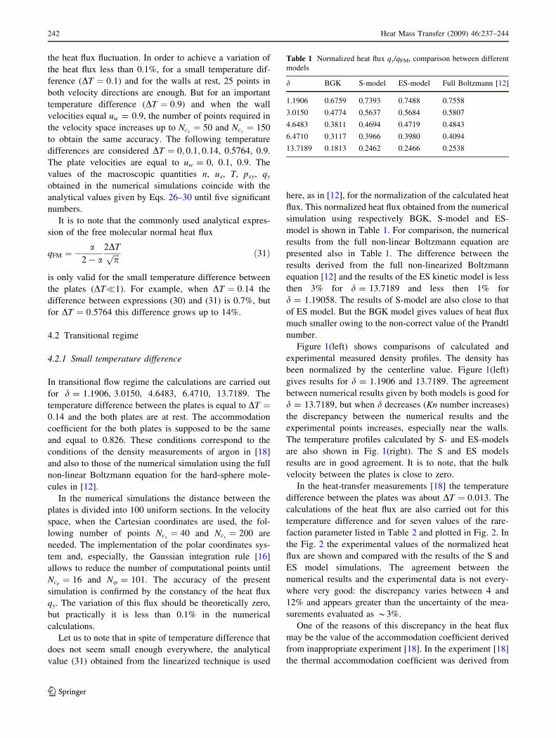
model is shown in Table 1. For comparison, the numerical
results from the full non-linear Boltzmann equation are
presented also in Table 1. The difference between the
results derived from the full non-linearized Boltzmann
equation [12] and the results of the ES kinetic model is less
then 3% for d = 13.7189 and less then 1% for
d = 1.19058. The results of S-model are also close to that
of ES model. But the BGK model gives values of heat flux
much smaller owing to the non-correct value of the Prandtl
number.
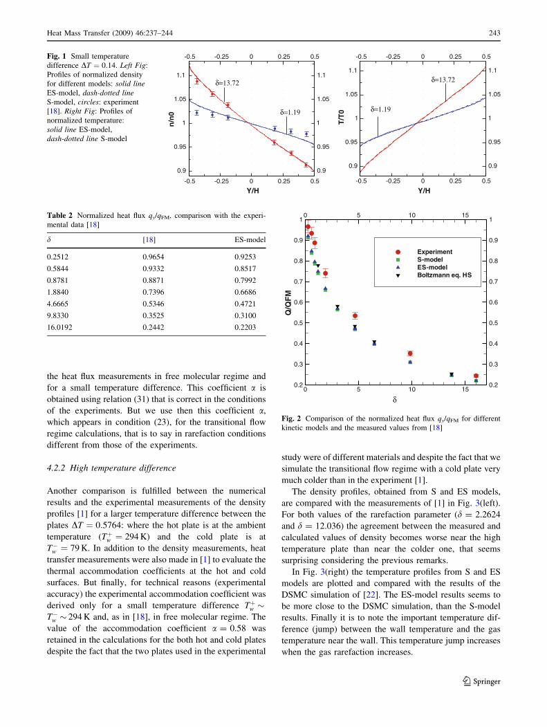
Figure 1(left) shows comparisons of calculated and
experimental measured density profiles. The density has
been normalized by the centerline value. Figure 1(left)
gives results for d = 1.1906 and 13.7189. The agreement
between numerical results given by both models is good for
d = 13.7189, but when d decreases (Kn number increases)
the discrepancy between the numerical results and the
experimental points increases, especially near the walls.
The temperature profiles calculated by S- and ES-models
are also shown in Fig. 1(right). The S and ES models
results are in good agreement. It is to note, that the bulk
velocity between the plates is close to zero.
In the heat-transfer measurements [18] the temperature
difference between the plates was about DT ¼ 0:013. The
calculations of the heat flux are also carried out for this
temperature difference and for seven values of the rare-
faction parameter listed in Table 2 and plotted in Fig. 2. In
the Fig. 2 the experimental values of the normalized heat
flux are shown and compared with the results of the S and
ES model simulations. The agreement between the
numerical results and the experimental data is not every-
where very good: the discrepancy varies between 4 and
12% and appears greater than the uncertainty of the mea-
surements evaluated as *3%.
One of the reasons of this discrepancy in the heat flux
may be the value of the accommodation coefficient derived
from inappropriate experiment [18]. In the experiment [18]
the thermal accommodation coefficient was derived from
Table 1 Normalized heat flux qy/qFM, comparison between different
models
d BGK S-model ES-model Full Boltzmann [12]
1.1906 0.6759 0.7393 0.7488 0.7558
3.0150 0.4774 0.5637 0.5684 0.5807
4.6483 0.3811 0.4694 0.4719 0.4843
6.4710 0.3117 0.3966 0.3980 0.4094
13.7189 0.1813 0.2462 0.2466 0.2538
242 Heat Mass Transfer (2009) 46:237–244
123
the heat flux measurements in free molecular regime and
for a small temperature difference. This coefficient a is
obtained using relation (31) that is correct in the conditions
of the experiments. But we use then this coefficient a,
which appears in condition (23), for the transitional flow
regime calculations, that is to say in rarefaction conditions
different from those of the experiments.
4.2.2 High temperature difference
Another comparison is fulfilled between the numerical
results and the experimental measurements of the density
profiles [1] for a larger temperature difference between the
plates DT ¼ 0:5764: where the hot plate is at the ambient
temperature (Tþw ¼ 294 K) and the cold plate is at
T�w ¼ 79 K. In addition to the density measurements, heat
transfer measurements were also made in [1] to evaluate the
thermal accommodation coefficients at the hot and cold
surfaces. But finally, for technical reasons (experimental
accuracy) the experimental accommodation coefficient was
derived only for a small temperature difference Tþw �T�w � 294 K and, as in [18], in free molecular regime. The
value of the accommodation coefficient a = 0.58 was
retained in the calculations for the both hot and cold plates
despite the fact that the two plates used in the experimental
study were of different materials and despite the fact that we
simulate the transitional flow regime with a cold plate very
much colder than in the experiment [1].
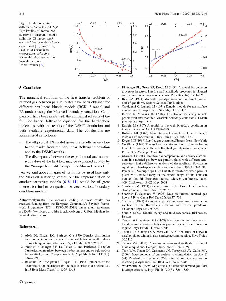
The density profiles, obtained from S and ES models,
are compared with the measurements of [1] in Fig. 3(left).
For both values of the rarefaction parameter (d = 2.2624
and d = 12.036) the agreement between the measured and
calculated values of density becomes worse near the high
temperature plate than near the colder one, that seems
surprising considering the previous remarks.
In Fig. 3(right) the temperature profiles from S and ES
models are plotted and compared with the results of the
DSMC simulation of [22]. The ES-model results seems to
be more close to the DSMC simulation, than the S-model
results. Finally it is to note the important temperature dif-
ference (jump) between the wall temperature and the gas
temperature near the wall. This temperature jump increases
when the gas rarefaction increases.
Y/H
n/n
0-0.5
-0.5
-0.25
-0.25
0
0
0.25
0.25
0.5
0.5
0.9 0.9
0.95 0.95
1 1
1.05 1.05
1.1 1.1δ=13.72
δ=1.19
Y/H
T/T
0
-0.5
-0.5
-0.25
-0.25
0
0
0.25
0.25
0.5
0.5
0.9 0.9
0.95 0.95
1 1
1.05 1.05
1.1 1.1
δ=13.72
δ=1.19
Fig. 1 Small temperature
difference DT ¼ 0:14. Left Fig:
Profiles of normalized density
for different models: solid lineES-model, dash-dotted lineS-model, circles: experiment
[18]. Right Fig: Profiles of
normalized temperature:
solid line ES-model,
dash-dotted line S-model
Table 2 Normalized heat flux qy/qFM, comparison with the experi-
mental data [18]
d [18] ES-model
0.2512 0.9654 0.9253
0.5844 0.9332 0.8517
0.8781 0.8871 0.7992
1.8840 0.7396 0.6686
4.6665 0.5346 0.4721
9.8330 0.3525 0.3100
16.0192 0.2442 0.2203
δ
Q/Q
FM
0
0
5
5
10
10
15
15
0.2 0.2
0.3 0.3
0.4 0.4
0.5 0.5
0.6 0.6
0.7 0.7
0.8 0.8
0.9 0.9
1 1
ExperimentS-modelES-modelBoltzmann eq. HS
Fig. 2 Comparison of the normalized heat flux qy/qFM for different
kinetic models and the measured values from [18]
Heat Mass Transfer (2009) 46:237–244 243
123
5 Conclusion
The numerical solutions of the heat transfer problem of
rarefied gas between parallel plates have been obtained for
different non-linear kinetic models (BGK, S-model and
ES-model) using the Maxwell boundary condition. Com-
parisons have been made with the numerical solution of the
full non-linear Boltzmann equation for the hard-sphere
molecules, with the results of the DSMC simulation and
with available experimental data. The conclusions are
summarized in follows:
– The ellipsoidal ES model gives the results more close
to the results from the non-linear Boltzmann equation
and to the DSMC results.
– The discrepancy between the experimental and numer-
ical values of the heat flux may be explained notably by
the ‘‘non-perfect’’ diffuse-specular Maxwell kernel.
As we said above in spite of its limits we used here only
the Maxwell scattering kernel, but the implementation of
another scattering models [6–8, 11] would be of great
interest for further comparison between various boundary
condition models.
Acknowledgments The research leading to these results has
received funding from the European Community’s Seventh Frame-
work Programme (ITN - FP7/2007-2013) under grant agreement
n 215504. We should also like to acknowledge J. Gilbert Meolans for
valuable discussions.
References
1. Alofs DJ, Flagan RC, Springer G (1970) Density distribution
measurements in rarefied gases contained between parallel plates
at high temperature difference. Phys Fluids 14(3):529–533
2. Andries P, Bourgat J-F, Le Tallec P, and Perthame B (2002)
Numerical comparison between the boltzmann and es-bgk models
for rarefied gases. Comput Methods Appl Mech Eng 191(31):
3369–3390
3. Bassanini P, Cercignani C, Pagani CD (1968) Influence of the
accommodation coefficient on the heat transfer in a rarefied gas.
Int J Heat Mass Transf 11:1359–1368
4. Bhatnagar PL, Gross EP, Krook M (1954) A model for collision
processes in gases. Part I: small amplitude processes in charged
and neutral one-component systems. Phys Rev 94(3):511–525
5. Bird GA (1994) Molecular gas dynamics and the direct simula-
tion of gas flows. Oxford Science Publications
6. Cercignani C, Lampis M (1971) Kinetic models for gas-surface
interactions. Transp Theory Stat Phys 1:101–114
7. Dadzie K, Meolans JG (2004) Anisotropic scattering kernel:
generalized and modified Maxwell boundary conditions. J Math
Phys 45(5):1804–1819
8. Epstein M (1967) A model of the wall boundary condition in
kinetic theory. AIAA J 5:1797–1800
9. Holway LH (1966) New statistical models in kinetic theory:
methods of construction. Phys Fluids 9(9):1658–1673
10. Kogan MN (1969) Rarefied gas dynamics. Plenum Press, New York
11. Nocilla S (1963) The surface re-emission law in free molecule
flow. In: Laurmann JA (ed) Rarefied gas dynamics. Academic
Press, New York, pp 327–346
12. Ohwada T (1996) Heat flow and temperature and density distribu-
tions in a rarefied gas between parallel plates with different tem-
peratures. Finite-difference analysis of the nonlinear Boltzmann
equation for hard-sphere molecules. Phys Fluids 8(8):2153–2160
13. Pantazis S, Valougeorgis D (2008) Heat transfer between parallel
plates via kinetic theory in the whole range of the knudsen
number. In: 5th European thermal-sciences conference, paper
409, Eindhoven, 18–22 May 2008
14. Shakhov EM (1968) Generalization of the Krook kinetic relax-
ation equation. Fluid Dyn 3(5):95–96
15. Sharipov F, Seleznev V (1998) Data on internal rarefied gas
flows. J Phys Chem Ref Data 27(3):657–706
16. Shizgal B (1981) A Gaussian quadrature procedure for use in the
solution of the Boltzmann equation and related problems.
J Comput Phys 41:309–328
17. Sone Y (2002) Kinetic theory and fluid mechanics. Birkhauser,
Boston
18. Teagan WP, Springer GS (1968) Heat-transfer and density-dis-
tribution measurements between parallel plates in the transition
regime. Phys Fluids 11(3):497–506
19. Thomas JR, Chang TS, Siewert CE (1973) Heat transfer between
parallel plates with arbitrary surface accommodation. Phys Fluids
16:2116
20. Titarev VA (2007) Conservative numerical methods for model
kinetic equations. Comput Fluids 36(9):1446–1459
21. Trott WM, Rader DJ, Gastaneda JN, Torczynski JR, Gallis MA
(2009) Measurements of gas-surface accommodation. In Abe T
(ed) Rarefied gas dynamic, 26th international symposium on
rarefied gas dynamics, vol 1084. AIP, New York
22. Wadsworth DC (1993) Slip effects in a confined rarefied gas. Part
I: temperature slip. Phys Fluids A 5(7):1831–1839
Y/H
n/n
(0)
-0.5
-0.5
-0.25
-0.25
0
0
0.25
0.25
0.5
0.5
0.8 0.8
1 1
1.2 1.2
1.4 1.4
1.6 1.6
1.8 1.8
δ=12.036
δ=2.2624
Y/H
T/T
0
-0.5
-0.5
-0.25
-0.25
0
0
0.25
0.25
0.5
0.5
0.6 0.6
0.8 0.8
1 1
1.2 1.2
1.4 1.4
δ=12.036
δ=2.2624
Fig. 3 High temperature
difference DT ¼ 0:5764. LeftFig: Profiles of normalized
density for different models:
solid line ES-model, dash-dotteded line S-model, circles:
experiment [18]. Right Fig:
Profiles of normalized
temperature: solid lineES-model, dash-dotted lineS-model, circles:
DSMC results [22]
244 Heat Mass Transfer (2009) 46:237–244
123