PNNL-13419

Comparison of Intake Gate Closure Methods at Lower Granite, Little Goose, Lower Monumental, and McNary Dams Using Risk-Based Analysis B. F. Gore H. K. Phan T. R. Blackburn D. M. Bardy P. G. Heasler R. E. Hollenbeck N. L. Mara January 2001 Prepared for the U.S. Army Corps of Engineers, Hydroelectric Design Center, Portland, OR and U.S. Army Corps of Engineers, Walla Walla District, Walla Walla, WA U.S. Department of Energy under Contract DE-AC06-76RL01830

DISCLAIMER This report was prepared as an account of work sponsored by an agency of the United States Government. Neither the United States Government nor any agency thereof, nor Battelle Memorial Institute, nor any of their employees, makes any warranty, express or implied, or assumes any legal liability or responsibility for the accuracy, completeness, or usefulness of any information, apparatus, product, or process disclosed, or represents that its use would not infringe privately owned rights. Reference herein to any specific commercial product, process, or service by trade name, trademark, manufacturer, or otherwise does not necessarily constitute or imply its endorsement, recommendation, or favoring by the United States Government or any agency thereof, or Battelle Memorial Institute. The views and opinions of authors expressed herein do not necessarily state or reflect those of the United States Government or any agency thereof. PACIFIC NORTHWEST NATIONAL LABORATORY operated by BATTELLE for the UNITED STATES DEPARTMENT OF ENERGY under Contract DE-AC06-76RL01830

This document was printed on recycled paper. (8/00)

PNNL-13419

Comparison of Intake Gate Closure Methods at Lower Granite, Little Goose, Lower Monumental, and McNary Dams Using Risk-Based Analysis B. F. Gore H. K. Phan1

T. R. Blackburn D. M. Bardy2

P. G. Heasler R. E. Hollenbeck3

N. L. Mara January 2001 Prepared for U.S. Army Corps of Engineers, Hydroelectric Design Center Portland, OR and U.S. Army Corps of Engineers, Walla Walla District, Walla Walla, WA

Pacific Northwest National Laboratory Richland, WA 99352

1 Energy Northwest, Richland, Washington 2 U.S. Army Corp of Engineers, Portland, Oregon 3 U.S. Army Corp of Engineers, Walla Walla, Washington

i

Summary Fish screen installation at hydroelectric stations, performed to divert migrating salmon from turbine inlets, has resulted in changes that prevent rapid closure of the intake gates that close off the dam pool from the turbine inlets. Some of the intake gates have been disengaged from hydraulic operating systems and raised, and in some cases hydraulic cylinders have been removed. If intake gate closure were required to terminate an over-speed or flooding event at a turbine-generator unit, the Corps of Engineers (COE) has estimated that up to six hours may be necessary at some plants. At the request of the COE, Pacific Northwest National Laboratory (PNNL) performed an analysis of the probability per year times estimated dollar consequences entailed by this situation. This risk analysis determined the events considered are credible, that some have happened, and a large financial risk is associated with powerhouses where intake gate closure requires six hours. Point estimates of the risk are about $2.5 million per year for small powerhouses and $6 million per year for large powerhouses. This risk estimate has a large uncertainty due to uncertainties in the basic data used in the analysis. The 5 percent lower uncertainty bounds are about a factor of 10 smaller than the point estimates, and the 95 percent upper bounds are about a factor of 3 higher than the point estimates. (The point estimates are closer to the upper bounds because the point estimates for basic data were obtained from the mean values of the data distribution functions. Mean values are expected to be larger than median values.) The risk analysis point estimate results indicated that modification of the intake gate closure system to allow 10-minute closure would provide a risk reduction of about $65 million per year for a large powerhouse (e.g. McNary), and almost $8 million per year for small powerhouses (e.g. Lower Monumental, Little Goose, and Lower Granite). The size of these potential benefits provided incentive to perform a detailed analysis of the benefits and costs associated with modifications necessary to accomplish 10-minute intake gate closure. The COE developed and provided to PNNL cost information for two types of systems capable of rapidly closing intake gates from the elevated positions where they are presently parked. A hydraulic system using 3-stage cylinders to achieve the necessary lift height was analyzed, as was a wire-rope hoist system. The analysis addressed capital cost of construction, periodic maintenance necessary for a 25-year operating lifetime, and annual maintenance costs of the new systems versus maintenance costs of the existing systems. Benefits (primarily risk reduction) were compared with costs through calculation of the net present value, and the benefit/cost ratio of the proposed modifications. The benefit-cost analysis found that both of the proposed systems are economically far superior to the present situation. The point value of the net present value of modifications to the large (McNary) powerhouse exceeded $760 million for both proposals. For the small powerhouses it exceeded $74 million for all cases. The point value of the benefit/cost ratio exceeded 10 for all but one case, with a maximum value of 32 for the hoist system at the large powerhouse. The results for the hoist system were somewhat better than for the hydraulic system, because its lower capital cost had a larger effect than its higher periodic maintenance costs. The analysis was based upon data gathered by a survey sent to powerhouses in the U.S. and Canada, supplemented by data gathered in expert elicitation workshops. These data were combined using Bayesian updating, resulting in a database having both point estimate and uncertainty information. The uncertainties in the basic data were used to calculate the uncertainties in the point estimates. For the benefit-cost analysis, the 5 percent lower uncertainty bound indicates that a small chance exists that costs will exceed benefits for all but the hoist system at the large (McNary) powerhouse. On the other hand, a

ii

small chance also exits of achieving benefit/cost ratios of 130 for McNary powerhouse, and of 40 for the other powerhouses. Based on the results of this study, upgrading the intake gate operators is recommended to allow closure within 10 minutes at Lower Granite, Little Goose, Lower Monumental, and McNary dams as a cost-effective way to reduce these risks. Based on the cost estimates and maintenance costs for the two competing solutions, the wire rope hoist is the most cost-effective approach to meet the closure criteria at these powerhouses. The results for these powerhouses do not necessarily translate to other plants in the Corps of Engineers. Each plant should be examined individually and a recommendation given based on the specifics of an individual plant. What can be asserted is that intake gate closure within 10 minutes is a supportable design goal. At plants where a minimal investment is required to achieve 10-minute closure, a decision to upgrade equipment can be supported easily.

1

Contents Summary.......................................................................................................................................................i

Figures...........................................................................................................................................................i

Tables .......................................................................................................................................................... ii

1 Introduction ......................................................................................................................................1

1.1 OBJECTIVE ......................................................................................................................................1 1.2 APPROACH ......................................................................................................................................2 1.3 SCOPE..............................................................................................................................................3 1.4 TERMINOLOGY, ABBREVIATIONS, AND DESIGN NUMBERING........................................................4

2 Risk Analysis Methodology, Results, and Conclusions .................................................................5

2.1 METHODOLOGY OVERVIEW............................................................................................................5 2.2 TIME-BASED RELIABILITY ANALYSIS ............................................................................................9

2.2.1 System Model Development.....................................................................................................9 2.2.2 Initiating Event Frequencies .................................................................................................14 2.2.3 Database Development..........................................................................................................15 2.2.4 Event Frequency Profiles, f(t) ...............................................................................................17

2.3 CONSEQUENCE ANALYSIS ............................................................................................................23 2.3.1 Damage State Probabilities, D(t) ..........................................................................................23 2.3.2 Damage State Cost Development ..........................................................................................37 2.3.3 Economic Consequence Analysis ..........................................................................................44

2.4 RISK ANALYSIS RESULTS AND CONCLUSIONS .............................................................................48 2.4.1 Risk Point Estimate Results and Conclusions .......................................................................52 2.4.2 Risk Uncertainty Analysis Results and Conclusions .............................................................56

3 Uncertainty Analysis Methodology...............................................................................................60

3.1 MONTE CARLO SIMULATION ........................................................................................................60 3.2 LATIN HYPERCUBE SAMPLING .....................................................................................................60 3.3 DISTRIBUTION FUNCTIONS USED..................................................................................................61

4 Benefit-Cost Analysis .....................................................................................................................62

4.1 METHODOLOGY ............................................................................................................................62 4.2 BENEFIT-COST RESULTS AND CONCLUSIONS...............................................................................64

5 Recommendations ..........................................................................................................................68

References ..................................................................................................................................................70

Appendix A. Basic Event Failure Data................................................................................................ A-1

Appendix B. Initiating Event Trees ......................................................................................................B-1

Appendix C. System Failure Fault Trees ............................................................................................ C-1

Appendix D. Damage State Cost Estimate Inputs.............................................................................. D-1

Acronyms and Abbreviations......................................................................................................................i

2

i

Figures

2.1 Overall Project Process Used for Calculating Risk.............................................................7 2.2 Expert Elicitation Process Flow Diagram…………………………………………….….11 2.3 Overall Process Used to Develop the Project Database……………………………....….12 2.4 Event Frequency Profiles for the Lower Monumental Powerhouse Comparing

the Present Situation with Expected Results for Proposed Modifications…………...…..20

2.5 Event Frequency Profiles Comparing Hydraulic and Crane Operated Intake Gate Designs, and Comparing Hydraulic Designs With and Without Fish Screens……………………………………………………………………………….......21

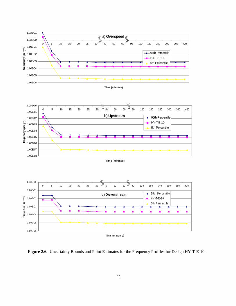
2.6 Uncertainty Bounds and Point Estimates for the Frequency Profiles for Design HY-T-E-10 …………………………………………………............................................22

2.7 Overall Process Used to Calculate Damage State Probabilities as a Function of Time……………………………………………………………………………..….....25

2.8 Schematic Layout of Representative Columbia and Snake River Powerhouse…....….…26 2.9 Damage State Cost Estimation Process………………………………………….....……37 2.10 Cumulative Amount of Energy Foregone and Value of Energy as a Function

of Number of Units Out-of-Service for the Small Powerhouse Model…………....…....39

2.11 Upstream Flooding Expected Costs and Uncertainty Bounds as a Function of Time................…………………………………………………………………......…49

2.12 Downstream Flooding Expected Costs and Uncertainty Bounds as a Function of Time ...............…………………………………………………………………….......50

2.13 Over-speed Expected Costs and Uncertainty Bounds as a Function of Time..................51

2.14 Uncertainty Bounds, Point Estimates, Mean, and Median Values of the Estimated Risks for the Small Powerhouse Model $/unit-yr....……….......…………………….......58

2.15 Uncertainty Bounds, Point Estimates, Mean, and Median Values of the Estimated Risks for the Large Powerhouse Model $/unit-yr.......…………………………….......…59

4.1 Point Estimates and Uncertainty Bounds of the Estimated Net Present Value for the Proposed Powerhouse Modifications……………………………………….........65

4.2 Point Estimates and Uncertainty Bounds for the Estimated Benefit/Cost Ratio for the Proposed Powerhouse Modifications……………………………………........….66

ii

Tables

1.1 Closure System Design Variants Addressed in This Study, and Correlation With Previous Design Numbers…………………………………………………………………5

2.1 Plant Systems of Interest for Study………………………………………………………10 2.2 Expert Panel Members – December 1994……………………………………………….11 2.3 Expert Workshop Participants – March 1995……………………………………………13 2.4 Expert Workshop Participants – August 1998…………………………………………..13 2.5 Contributions to the Over-speed Initiating Event Frequency (events/unit-yr.)………….14 2.6 Contributions to the Upstream Flooding Initiating Event Frequency (events/unit-yr.)….15 2.7 Contributions to the Downstream Flooding Initiating Event Frequency

(events/unit-yr.)………………………………………………………………………......15

2.8 Expert Workshop Participants – June 1995……………………………………………...24 2.9 Flooding Damage State Definitions……………………………………………………...26 2.10 Over-speed Mechanical Damage State Definitions……………………………………...27 2.11 Upstream Flooding Source Probability Apportionment………………………………....28 2.12 Downstream Flooding Source Probability Apportionment……………………………...29 2.13 Over-speed Flooding Source probability Apportionment………………………………..30 2.14 Sizes and Shapes of Leaks Assumed for Flooding Calculations, the Initial

Hydraulic Head Across the Leak, and Initial Flow Rates………………………………..31

2.15 Volumes Assumed for Small and Large Powerhouse Leaks (1000 ft3)………………….32 2.16 Times Required for Flooding to Reach Each Damage State for Small and Large

Powerhouse Models……………………………………………………………………...32

2.17 Upstream Flooding Matrixes for Small and Large Plants……………………………….33 2.18 Downstream Flooding Matrixes for Small and Large Plants…………………………….33 2.19 Over-speed Flooding Matrixes for Small and Large Plants……………………………...33 2.20 Expert Estimates and Linear Interpolation of Over-speed Damage State

Probabilities, Uncertainties in the Estimates, and the Probabilities of Flooding Initiation as a Consequence of the Damages…………………………………………….34

iii

2.21 Over-speed Without Flooding Damage State Probability Matrix………………………..35 2.22 Over-speed With Flooding Damage State Probability Matrix for Small Powerhouse Model……………………………………………………………………….36 2.23 Over-speed With Flooding Damage State Probability Matrix for Large

Powerhouse Model…………………………………………………………………….…36 2.24 Estimated Time-Out-of-Service by Damage State for the Small Powerhouse Model…...40 2.25 Estimated Time-Out-of-Service by Damage State for the Large Powerhouse Model…...41 2.26 Damage State Costs for the Small Powerhouse Model………………………………….43 2.27 Damage State Costs for the Large Powerhouse Model………………………………….44 2.28 Upstream Flooding Expected Damage State Costs and Total Expected Costs as

a Function of Time (Dollars)…………………………………………………………….45

2.29 Downstream Flooding Expected Damage State Costs and Total Expected Costs as a Function of Time (Dollars)…………………………………………………………….46

2.30 Over-speed Expected Damage State Costs and Total Expected Costs as a Function of Time (Dollars)………………………………………………………….…47

2.31 Total Risk Point Estimates for the Small Powerhouse Model ($M/unit-yr.)…………....52 2.32 Total Risk Point Estimates for the Large Powerhouse Model ($M/unit-yr.)………..…..52 2.33 Estimated Risk Components for the Small Powerhouse Model…………………………54 2.34 Estimated Risk Components for the Large Powerhouse Model…………………………55 2.35 Uncertainty Bounds (5 and 95 percentile values) of the Estimated Total Risks for

Small Powerhouse Model ($M/unit-yr.)……………………………………………...….56

2.36 Uncertainty Bounds (5 and 95 percentile values) of the Estimated Total Risks for Large Powerhouse Model ($M/unit-yr.)………………………………………………....57

4.1 Modifications Proposed for Hydroelectric Station Intake Gate Operating Systems…….62 4.2 Values Input into the Calculations of Net Present Value and Benefit/Cost Ratio ($ Million)………………………………………………………………………………..64 4.3 Uncertainty Bounds, Point Estimates, Mean, and Median Values of the Estimated Net Present Value for the Proposed Powerhouse Modifications………………………...67 4.4 Uncertainty Bounds, Point Estimates, Mean, and Median Values of the Estimated Benefit/Cost Ratio for the Proposed Powerhouse Modifications………………………..67

iv

4.5 Present Values of the Components of the Net Present Value and Benefit/Cost

Calculations ($ Million)……………………………………………………………….....68

1

1 Introduction Fish screen installation at hydroelectric stations on the Columbia and Snake Rivers was performed to divert migrating salmon from turbine inlets. Installation of fish screens has resulted in changes that prevent rapid closure of the intake gates that close off the dam pool from the turbine inlets. Guidance by the U.S. Army Corps of Engineers (COE) specifies that in an emergency the intake gates should be capable of closure within 10 minutes (the 10-minute rule). As originally designed, the intake gates are operated by hydraulic cylinders for an emergency closure that meets the 10-minute criteria required in EM 1110-2-4205. In order to utilize the intake gates for emergency closure to meet this criteria, new extended length hydraulic cylinders or wire rope systems would have to be installed at each of the four projects. The initial estimate in the early 1990s for modifications to Walla Walla District projects was approximately $42 million. An alternative closure system was proposed that identified a tremendous cost savings. This system would utilize the wicket gates, with a nitrogen charged backup system should loss of governor oil pressure occur, as initial closure under emergency conditions. The intake gates would be dogged off in the top of the intake gate slot with quick-connect hydraulic couplings. After the wicket gates were closed, the intake gates would be moved to the appropriate location in the slot, the hydraulics connected, cylinders reinstalled, and the intake gate deployed. Reconnecting the cylinders would take approximately 4 to 8 hours depending on the response time of emergency crews and the project location. An issue of concern is the reliability of the wicket gates during a runaway turbine event, and the ability of the wicket gates to close as a result of loss of governor oil pressure. Field tests confirmed that most of the wicket gates would move to the speed-no-load position during an over-speed event with the loss of governor oil pressure. Initial closure time is approximately 10 seconds. However, although it was determined that wicket gate closure is suited for some head cover failures, failed access hatch, abnormal operation and some limited wicket gate failures, some events are not controlled by wicket gate closure alone. Concern arises with the frequency of events that would require an emergency closure, and risks associated with the reliability of the wicket gates. Therefore, it was recommended that a risk analysis of this system be performed to evaluate the existing condition in comparison to upgraded intake gate operators. Approval was given to the Walla Walla District for the alternate closure system for Little Goose and Lower Granite Dams on 26 December 1989. A request to operate Lower Monumental Dam and McNary Dam using the alternate closure system was not granted. However, McNary Dam was granted a waiver from Corps Headquarters to use an interim system to meet critical installation of the new screens. The results of this study will be used to support a final recommendation for these plants. The risk analysis performed by PNNL indicated a substantial financial risk associated with delayed closure of intake gates, as compared with ability to meet the 10-minute rule. In this report, risk is a financial quantity that is specified in terms of expected dollar loss per year of operation. Consequently, the adjective financial is not used to modify risk in the rest of the report. To better understand this large risk, the COE asked PNNL to perform a detailed economic analysis comparing the benefits of being able to meet the 10-minute rule with the costs of necessary modifications.

1.1 Objective The objective of this report is to compare the benefits and costs of modifications proposed for intake gate closure systems at four hydroelectric stations on the Lower Snake and Upper Columbia rivers in the Walla Walla District that are unable to meet the COE 10-minute closure rule due to the installation of fish

2

screens. The primary benefit of the proposed modifications is to reduce the risk of damage to the station and environs when emergency intake gate closure is required. Consequently, this report presents the methodology and results of an extensive risk analysis performed to assess the reliability of powerhouse systems. The report also includes the costs and timing of potential damages resulting from events requiring emergency intake gate closure. As part of this analysis, the level of protection provided by the nitrogen emergency closure system was also evaluated. The nitrogen system was the basis for the original recommendation to partially disable the intake gate systems. The risk analysis quantifies this protection level.

1.2 Approach The COE provided design and cost information to PNNL for two different potential modifications to the existing intake gate closure systems. Both proposed modifications would park the intake gates in the present, raised configuration, yet allow closure in 10 minutes when required. One proposed system used 3-stage hydraulic cylinders to obtain the lift height required; the other one used a wire rope hoist to raise and lower the intake gates. Costs and benefits were converted to present values for comparison according to standard methods. The primary benefit of the proposed modifications is the reduction of risks to the powerhouse and environs achieved by rapid intake gate closure. Quantification of these benefits required development of a risk analysis methodology that includes an explicit, detailed analysis of the time evolution of events following their initiation. This analysis methodology was necessary because damage increases with time during the emergency events considered. The longer the time between event initiation and termination, the greater the resulting damage and its associated cost. The risk measure used in this study is the probable cost of the events, computed as the product of event frequency (per year) times cost summed over the possible duration of event propagation (assumed to be up to 8 hours after event initiation). Consequently, the units of risk are dollars per year. The study addressed generator loss of load events that could lead to turbine over-speed, and powerhouse flooding events that could be terminated by intake gate closure. Flooding caused by damage due to over-speed events was evaluated, as was flooding due to hatch failures upstream of the wicket gates (scroll case) and downstream of them (draft tube). The risk associated with any event may be thought of as the risk of event initiation and propagation until wicket gate actuation, plus the risk that wicket gates fail to stop water flow and the event propagates until intake gate actuation, plus the risk that intake gates fail to stop water flow and the event continues to propagate for a total of 8 hours. The methodology incorporates a variety of operator recovery actions that may occur at intermediate times, so the algorithm for evaluating risk is complicated. Nevertheless, the success or failure of wicket and intake gate actuation, combined with the time duration of event propagation until these actuations, are primary determinants of risk. Powerhouse size is also an important determinant of risk because powerhouse volume affects the speed of water level rise during flooding and also affects the number of units damaged. The COE provided cost and time estimates for the work required to repair damages, plus data and the methodology for computing the costs of lost power generation during repairs. A database of component failure frequency information was developed for this study, based on information gathered in a survey of U.S. and Canadian hydroelectric facilities, and also on expert elicitation workshops. Point estimates and probability distribution functions were developed for each of

3

the basic events evaluated. The analysis provided, in addition to point estimates of risks, benefits and costs, an uncertainty analysis that yielded uncertainty bounds for each of the point estimates.

1.3 Scope The risk analysis portion of this study was performed first in order to determine the reliability of the systems involved, the potential financial consequences of system failure, and the magnitude of the risk resulting from inability to meet the 10-minute rule. Consequently, the scope of the risk analysis was considerably broader than the scope of the benefit/cost analysis (that focused on proposed modifications to four powerhouses). The risk analysis methodology was applied to 12 different system designs, and to 3 different cases (times of intake gate operation) for each design. It was also applied to two different powerhouse sizes representative of the large and small powerhouses (14- and 6-turbine/generator units, respectively) on the Columbia and Snake rivers. This application results in a large array of results. One secondary objective of this report is to present the information in a logical, comprehensive manner to facilitate understanding the primary factors that determine the results. As a consequence, the presentation and discussion of powerhouse design features is different from that used in previous, preliminary reports of work performed. Nevertheless, the design and case numbering scheme used previously is retained to allow traceability. Unfortunately, the previously used design numbering system does not correlate with the organization of the design features discussed. The primary variant for comparison of the designs is the type of operating system for the intake gates. Hydraulic and gantry crane-operated intake gate systems are compared in the risk analysis. Certain hydraulic systems are able to close the intake gates within 10 minutes of an initiating event, whereas 30 minutes is estimated for crane-operated systems. However, not all hydraulic systems can achieve 10-minute closures. In some cases, intake gates are resting on dogs, and must be lifted and the dogs retracted before the gates can be lowered. This results in a 20- to 30-minute closure time. In other cases, gates have been raised above the normal operating range, and the hydraulic cylinders removed, or gates and cylinders both have been removed. This change results in a 6-hour closure time. This latter situation is the case for the systems for which modifications are proposed and for which benefit/cost analyses are addressed in this study. Two variants have been proposed for the modifications, both capable of closing in 10 minutes – one is a 3-stage hydraulic system, and the other is a wire rope hoist system. The analyses reported here, and in previous reports, address these three cases for each hydraulic design variant; 10-minute, 30-minute, and 6-hour closure times (identified as cases 1, 2, and 3 in previous reports). Crane operated systems can close the intake gates in 30 minutes if the gantry crane is already positioned above the unit that must be shut down, with the gates already suspended on the crane and ready for installation. If the crane must be moved, intake gate closure will require 60 minutes. If the gates have been taken off the crane (for instance to allow use of the crane for some type of maintenance), intake gate closure is estimated to require 6 hours. Consequently, for crane operated systems the cases addressed are 30-minute, 60-minute, and 6-hour closure times. (These were identified as cases 1, 2 and 3 in previous reports. Note the timing of cases 1 and 2 differs from the timing for hydraulic systems.) The second variant for comparison of the designs is whether or not fish screens have been installed to divert fish from the intakes of the turbines, and the type of fish screen installed, if screens are present. This information is important because fish screens can and do fail, resulting in the possibility of debris interfering with the operation of wicket gates or intake gates. Two types of fish screens are considered in this study, traveling mesh fish screens (TMFS) and fixed bar fish screens (FBFS). Because differing

4

failure rates have been experienced for the two types of fish screens, different risks are predicted for designs with one or the other, and for designs without fish screens. The third variant for comparison of the designs is the presence or absence of a nitrogen emergency closure system for the wicket gates. This system provides nitrogen under pressure that is injected into the oil system to pressurize it and operate the wicket gate servomotors, if the governor system controlling wicket gate position fails. The function of the emergency closure system is to improve the reliability of wicket gate closure and, presumably, reduce risks.

1.4 Terminology, Abbreviations, and Design Numbering For convenience in referring to the various closure system design variations discussed in this document, the following nomenclature is introduced to allow an abbreviated description of each design variation. Intake Gate Operating System: • Hydraulic – HY • Hoist-operated – HO • Crane-operated – CR Fish Screen Type: • Traveling mesh fish screen – T • Fixed Bar Fish Screen – F • No fish screen – N Emergency Closure System (Nitrogen): • Exists – E • None – (blank) Time of Intake Gate Closure Considered: • Ten minutes – 10 • Thirty minutes – 30 • Sixty minutes – 60 • Six hours – 360 Table 1.1 identifies the design variations analyzed for this report, and also provides the design identifying number used in previous reports of work done for this project. Note that case identification (minimum time of intake gate operation) is not included in the table, nor is powerhouse size.

5

Table 1.1. Closure System Design Variants Addressed in This Study, and Correlation with Previous Design Numbers Hydraulic I.G. Systems Hoist-Operated I.G. Systems Crane-Operated I.G. Systems HY-N (Design 11) CR-N (Design 12) HY-T (Design 3) CR-T (Design 4) HY-F (Design 7) CR-F (Design 8) HY-T-E (Design 15) HO-T-E (Design 14 or 50) CR-T-E (Design 16) HY-F-E (Design 19) HO-F-E (Design 18 or 49) CR-F-E (Design 20)

2 Risk Analysis Methodology, Results, and Conclusions A unique methodology was developed for the analysis of risk that explicitly incorporates the time dependence of event evolution following its initiation. Three types of events were considered: • Over-speed (causing direct equipment damage and flooding resulting from the damages) • Upstream flooding (from a leak/rupture upstream of the wicket gates) • Downstream flooding (from a leak/rupture downstream of the wicket gates). The explicit incorporation of time dependence was necessary because damages resulting from over-speed and flooding increase with time in a complex way. Furthermore, the course of each event is subject to modification or termination as a result of actions performed by control systems (e.g. governors) and by operators. Consequently, it was necessary to model in detail the evolution of each initiating event. The developed model addresses not only the probability of success of the various recovery actions and the damages that accumulated up to the time of each recovery action, but also the probability of recovery action failure and of subsequent damages that would result following the possible failure.

2.1 Methodology Overview The risks associated with events requiring non-routine shutdown of a hydroelectric station were estimated by combining information according to the flow chart presented in Figure 2.1. Risk is estimated by combining event frequency (annual probability of occurrence) information with event consequence information. Risk is defined by the formula (McCormick 1981):

EAR *= (2.1) where R = risk

A = estimated annual probability of a damaging event E = estimated cost of damage.

For the hydroelectric facilities in this study, the risk (R) was calculated for 30 possible damage conditions (states) that can result from the initiating events. Consequently, equation 2.1 was modified to include the risks from all of the individual damage-states:

6

∑=

=I

iii EAR

1

* (2.2)

where Ai = estimated annual probability of damaging events for the ith damage-state

Ei = estimated cost of being in the ith damage-state I = total number of damage-states i = individual damage-states.

Equation 2.2 was then further modified to incorporate the time dependence of event development. It is instructive to review the flow chart of the risk evaluation process (Figure 2.1) to understand the modification. First, an event frequency function f(t) was defined that provides the probability per year of each initiating event [f(t=0) is the initiating event frequency]. The time development of f(t) was determined by multiplying f(0) successively by the estimated probability of failure of each of the recovery actions at the time of its occurrence. This procedure results in a function that is maximum at t = 0, and decreases continually thereafter as time increases. Finally, f(t) was changed by discretization into 17 sequential time steps ranging between 5 minutes (initially) and 1 hour (later in the event), spanning a total of 420 minutes. The estimation of the consequences C(t) of an event used a probabilistic approach. For flooding events, multiple leak/rupture sizes were postulated and probabilities assigned to each. A similar approach was used to address the mechanical and flooding damages of over-speed events, with flooding allowed to initiate and increase as the over-speed event continued. Damage states were defined based on the depth of flooding in the various levels of the powerhouses and on the extent of mechanical damage expected from over-speed events of varying severity. Flooding damage, as a function of time, was estimated based on flow rates calculated from leak/rupture area, shape, and the hydraulic pressure across the leak. This process resulted in time-dependent damage state probability matrixes D(t). The costs associated with each damage state (construction, environmental, interest, and lost-power generation costs) were estimated and multiplied by the damage state probability matrixes, resulting in time-dependent consequence matrixes C(t). The C(t) were changed by discretization into 17 sequential time steps, just as f(t) were changed.

7

Event Frequency

f(t) Damage State Cost

E Damage State Probability

D(t)

Consequence C(t)

Risk R

Phase 1Data

(Component Reliability)

SystemLogic (Fault Trees)

Overspeed and F looding

Event Processes

(Event Trees)

Component Tim ing

Information RecoveryActions

Failure Com binations(Risk AssessmentSoftware Cut sets)

Phase 2Frequency

Profiles

Flooding Dam age State Probabilities Over-speed Dam age State Probabilities

Facility and F looding Source Characteristics

Downstream Flooding

Dam age S tate Probab ility

Matrix

Upstream Flooding

Dam age S tate Probab ility

Matrix

Over-speed Dam age S tate

Probab ility Matrix

Expert Over-speed Dam age S tate

Estim ates

Over-speed Flooding

Dam age S tate Probab ility

Matrix

Over-speed with Flooding

Dam age S tateProbab ility

Matrix

ConstructionCosts

(Flooding and Overspeed)

Environm ental Costs

Interest Costs

Costs for Damage States

Combines Damage State Costs and Probabilities to

Produce ConsequenceCurves

Combines Frequency Profiles with

Consequence Curves produce Risk values

Damage StateProbabilityMatrixes

Lost Power Generation

Costs

Figure 2.1. Overall Project Process Used for Calculating Risk

7

8

The risk, in dollars per unit-year, was then estimated by combining the estimated event frequency information, f(tk) with the estimated economic consequences C(tk), using Equation 2.3 .

[ ])()(2

)()(1

17

1

1+

=

+ −

+= ∑ kk

k

kk tftftCtC

R (2.3)

where R = calculated risk C(tk) = estimated consequence at time step k C(tk+1) = estimated consequence at time step k+1 f(tk) = estimated event frequency at time step k f(tk+1) = estimated event frequency at time step k+1 To understand this equation, remember that f(t) can only decrease as t increases. Also, note that at any time step where f(t) does not decrease, zero contribution to the risk sum results, and consequences continue to accumulate due to flooding and mechanical damage. When a recovery action does reduce f(t), the decrement of frequency is multiplied by the consequences that have accumulated until that time (averaged over the last time step), and added to the risk sum. However, a probability remains for the event not to be terminated successfully that is captured in the reduced subsequent value of f(t). The possible consequences continue to accumulate until another recovery action again reduces f(t), and another contribution is added to the risk sum. The summation continues to accumulate until f(t) is set to zero at 480 minutes after event initiation; thus, it is assumed that all events are terminated 8 hours after initiation. This risk calculation is performed separately for upstream flooding event sequences, downstream flooding sequences, and over-speed sequences. The results from these three risk calculations are summed to obtain the total risk estimation attributed to flooding and over-speed event sequences that require non-routine shutdown at a hydroelectric station. Because different economic consequence estimations arise for a small (6-unit) hydroelectric station and a large (14-unit) one, the individual event sequence risk estimations and total risk estimation are presented for both small and large hydroelectric stations. The analyses have been made for a variety of different representative hydroelectric station design types, and therefore the risk estimations are presented for each one of the station design types evaluated. This methodology was used to calculate point estimates of risk for the various powerhouse designs and sizes analyzed. This was done using point estimates of the frequencies and failure probabilities of components of the various systems studied to determine f(t) and the damage extent and costs captured in C(t). The point estimates used were the mean values of the distribution functions of the failure probabilities and the frequencies determined from data obtained using surveys and an expert elicitation process. This methodology also was used to perform an uncertainty analysis of the results. A Monte Carlo approach was used, with Latin Hypercube sampling of the data distribution functions for each of the events in the database. This approach includes not only component failure rates, but damage estimates, cost to repair estimates, and cost of replacement power estimates. A sample size of 200 was used; thus the output for each design and case analyzed was 200 values of risk clustered randomly about the point estimate values. The risk values were ordered according to size, and the 10 largest and 10 smallest were discarded. The spread of the remaining values was used to specify 5 percent and 95 percent uncertainty

9

bounds for the results. Mean and median values of the 200 risk values were also calculated to allow comparison of the point values with the distribution of results. Due to the wide spread of the distribution functions for much of the data, mean values of the risk distribution often were larger than the point estimates computed using the mean values of the individual data.

2.2 Time-Based Reliability Analysis The first step in powerhouse risk calculation is the analysis of the reliability of the systems used to terminate an initiating event to determine their likelihood of success or failure when called upon. This analysis results in the development of the event frequency function f(t) shown in Figure 2.1 and used in Equation 2.3. Standard fault tree and event tree methods were used to evaluate the frequencies of events requiring non-routine shutdowns that might require (and would be terminated by) intake gate closure. These methods were used to evaluate the combinations of component failures that could lead to initiating events, subsequent failures to the closure of the wicket gates, and eventual failures of the intake gates to close and terminate the event. This evaluation required development of system logic models and a database of component failure rates for the various systems and components involved. The system logic models were combined to determine the overall probability of water flow being terminated as a function of time following an initiating event. This process required the explicit incorporation of time into the modeling and analysis. Standard risk analysis methods were used to determine the many combinations of component failures in the various systems that could lead to complete failure in terminating water flow. Computer coding was used to evaluate and sum the probabilities of these component failure combinations as a function of time following an initiating event. This coding included the explicit evaluation of whether each system was capable of operating at each time step and, hence, whether each component could have contributed to the success or failure of water flow termination. Thus, 5 minutes after an initiating event, the wicket gate system could have acted; the probability that water flow would not be terminated was calculated using the failure probabilities of the various components in the wicket gate system. The mitigating effects of intake gate system components were ignored until a later time when that system could have acted. The effects of recovery actions taken by operators, following failure of a system to accomplish its mission, were also included in the models. The timing of recovery actions, and their likelihood of failure, was modeled to occur after a time delay appropriate to the system and action in question.

2.2.1 System Model Development The project began with site visits and a review of documents and drawings addressing the design, operation and maintenance of hydroelectric stations. It continued with development of a survey to gather data on the reliability of components belonging to the systems that perform the required functions. Many different types of powerhouse and system designs exist in the Northwest alone. Consequently, it was necessary to group and categorize the designs in such a way that system logic models could capture the most important design differences, yet result in a limited number of categories for subsequent detailed analysis. A design features matrix was developed defining 48 different design variants. These variations involve four different types of intake gate closure systems, two types of fish screens (or none), presence or absence of an emergency closure system for the wicket gates, and use of an electrical or mechanical governor for controlling the wicket gates and turbine blade positions. The design identification numbering system used in previous reports was derived from this matrix. This report uses the simplified nomenclature described in the Introduction and in Table 1.1 to identify the various designs so the nomenclature itself clearly identifies the design features. This nomenclature works because only 12 of the designs subsequently were analyzed during the course of the study.

10

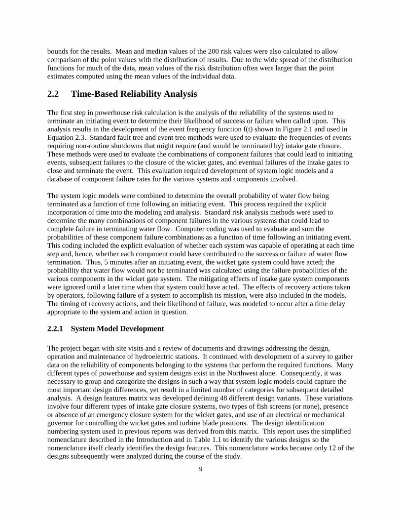
Development of the system models utilized an iterative approach. The information obtained during the initial plant visits and document reviews were studied to determine system function, physical description and layout, operation, and maintenance. This information was then used to develop preliminary logic models of system operation. Each model was analyzed to determine the information on system and component reliability necessary to support a risk and reliability analysis. Working meetings were then held with COE experts to review and revise the system models and the lists of needed data. Systems analyzed are listed in Table 2.1. Table 2.1. Plant Systems of Interest for Study

System # System

1 Trash Rack 2 Intake Gate (Gantry Crane Mechanism) 3 Intake Gate (Gate Mechanism) 4 Intake Gate (Hoist Mechanism) 5 Intake Gate (Hydraulic System) 6 Intake Valve 7 Penstock, Scroll Case, Draft Tube 8 Wicket Gate 9 Main Unit Turbine Runner

10 Main Unit Turbine Shaft and Kaplan Mechanism 11 Main Generator 12 Main Unit Governor Wicket (Gate and Blades) 13 AC and DC Systems 14 Protection 15 Fish Screen and Vertical Barrier Screen

When it was determined that system models were sufficiently well developed, and the reliability data needed to analyze the models were adequately known, a survey questionnaire was developed and sent to 337 hydroelectric stations in the U. S. and Canada. The stations queried have either Kaplan or Francis turbines with ratings exceeding 25 MWe. The survey questions focused on obtaining historical data from the station that would be useful in analyzing the models developed for this project. Information was collected regarding initiating event frequencies, plant design and maintenance, and failures of individual systems and components. Each system addressed in the survey was defined through a concise description of the system function and system boundaries. Questions addressed basic system design and maintenance information, and the actual performance information of the system. Performance questions focused on potential system level malfunctions, failures or near miss events, and the frequency of occurrence. The questions were followed by ones addressing the detailed failure history of individual components, formatted as a failure modes and effects analysis (FMEA) table. The information obtained from these questions was used to quantify the failure probabilities of components included in the system logic models (fault trees). The information from each survey was assessed to ensure that it was representative and then entered into the database developed for the project. Following distribution of the survey questionnaires, a formal expert judgment elicitation workshop was conducted December 13 to 15, 1994 in Seattle, Washington. This workshop had two purposes: first, to validate the risk analysis model developed by PNNL, and second, to estimate failure data for hydro-

11

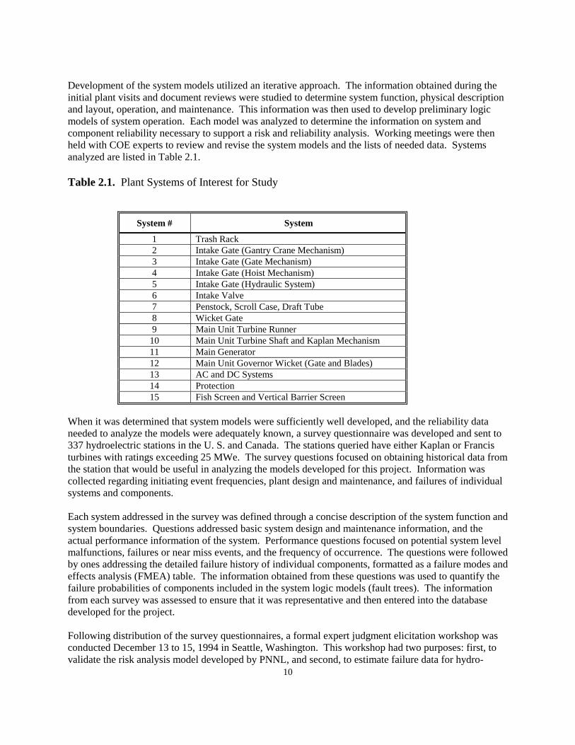
electric station components determined to be important in the model. The panel members and their areas of expertise are identified in Table 2.2. Table 2.2. Expert Panel Members – December 1994

Expert Name Expertise Company Name Location

Jim Bluhm Operations COE Walla Walla, WA Ron Darkes Operations PGE Portland, OR Steve Doret Design New England Power Service Company Westborough, MA Dan Drake Design Bureau of Reclamation Lakewood, CO Laurence Henry Field Service Hydraulic Turbine Consultants York, PA Bob Lee Operations Noregon Hydro Portland, OR Charles McKee Design Operations Chelan County PUD Wenatchee, WA Brian Moentenich Turbine Design COE, HDC Portland, OR Patrick Ryan Design Woodward Governor Company Stevens Point, WI James Sinclair Design Consulting Engineer Lynden, WA Larry Walker Operations COE Pasco, WA

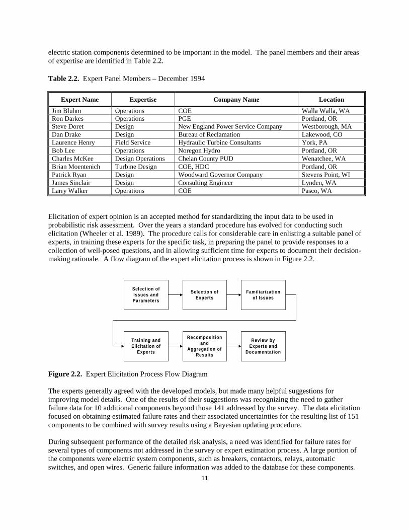
Elicitation of expert opinion is an accepted method for standardizing the input data to be used in probabilistic risk assessment. Over the years a standard procedure has evolved for conducting such elicitation (Wheeler et al. 1989). The procedure calls for considerable care in enlisting a suitable panel of experts, in training these experts for the specific task, in preparing the panel to provide responses to a collection of well-posed questions, and in allowing sufficient time for experts to document their decision-making rationale. A flow diagram of the expert elicitation process is shown in Figure 2.2.

Selection ofIssues andParameters

Selection ofExperts

Familiarizationof Issues

Training andElicitation of

Experts

Recompositionand

Aggregation ofResults

Review byExperts and

Documentation

Figure 2.2. Expert Elicitation Process Flow Diagram

The experts generally agreed with the developed models, but made many helpful suggestions for improving model details. One of the results of their suggestions was recognizing the need to gather failure data for 10 additional components beyond those 141 addressed by the survey. The data elicitation focused on obtaining estimated failure rates and their associated uncertainties for the resulting list of 151 components to be combined with survey results using a Bayesian updating procedure. During subsequent performance of the detailed risk analysis, a need was identified for failure rates for several types of components not addressed in the survey or expert estimation process. A large portion of the components were electric system components, such as breakers, contactors, relays, automatic switches, and open wires. Generic failure information was added to the database for these components.

12

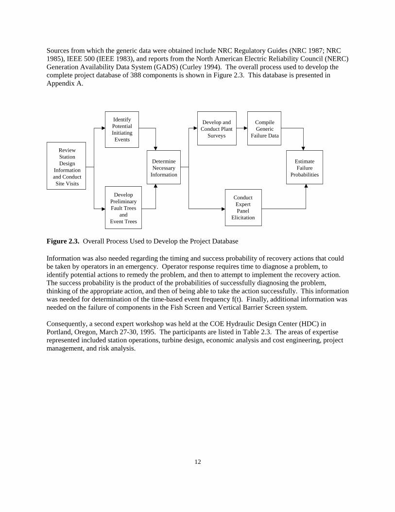
Sources from which the generic data were obtained include NRC Regulatory Guides (NRC 1987; NRC 1985), IEEE 500 (IEEE 1983), and reports from the North American Electric Reliability Council (NERC) Generation Availability Data System (GADS) (Curley 1994). The overall process used to develop the complete project database of 388 components is shown in Figure 2.3. This database is presented in Appendix A.

ReviewStationDesign

Informationand ConductSite Visits

IdentifyPotentialInitiatingEvents

DevelopPreliminaryFault Trees

andEvent Trees

DetermineNecessary

Information

Develop andConduct Plant

Surveys

CompileGeneric

Failure Data

ConductExpertPanel

Elicitation

EstimateFailure

Probabilities

Figure 2.3. Overall Process Used to Develop the Project Database

Information was also needed regarding the timing and success probability of recovery actions that could be taken by operators in an emergency. Operator response requires time to diagnose a problem, to identify potential actions to remedy the problem, and then to attempt to implement the recovery action. The success probability is the product of the probabilities of successfully diagnosing the problem, thinking of the appropriate action, and then of being able to take the action successfully. This information was needed for determination of the time-based event frequency f(t). Finally, additional information was needed on the failure of components in the Fish Screen and Vertical Barrier Screen system. Consequently, a second expert workshop was held at the COE Hydraulic Design Center (HDC) in Portland, Oregon, March 27-30, 1995. The participants are listed in Table 2.3. The areas of expertise represented included station operations, turbine design, economic analysis and cost engineering, project management, and risk analysis.

13

Table 2.3. Expert Workshop Participants - March, 1995

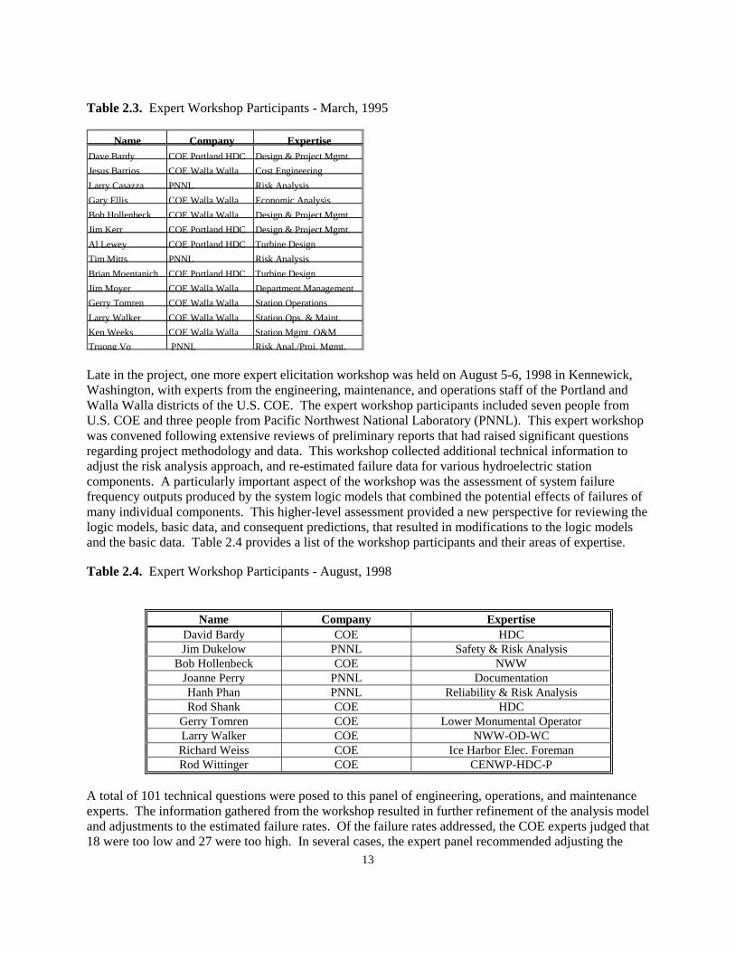
Late in the project, one more expert elicitation workshop was held on August 5-6, 1998 in Kennewick, Washington, with experts from the engineering, maintenance, and operations staff of the Portland and Walla Walla districts of the U.S. COE. The expert workshop participants included seven people from U.S. COE and three people from Pacific Northwest National Laboratory (PNNL). This expert workshop was convened following extensive reviews of preliminary reports that had raised significant questions regarding project methodology and data. This workshop collected additional technical information to adjust the risk analysis approach, and re-estimated failure data for various hydroelectric station components. A particularly important aspect of the workshop was the assessment of system failure frequency outputs produced by the system logic models that combined the potential effects of failures of many individual components. This higher-level assessment provided a new perspective for reviewing the logic models, basic data, and consequent predictions, that resulted in modifications to the logic models and the basic data. Table 2.4 provides a list of the workshop participants and their areas of expertise. Table 2.4. Expert Workshop Participants - August, 1998

Name Company Expertise

David Bardy COE HDC Jim Dukelow PNNL Safety & Risk Analysis

Bob Hollenbeck COE NWW Joanne Perry PNNL Documentation Hanh Phan PNNL Reliability & Risk Analysis Rod Shank COE HDC

Gerry Tomren COE Lower Monumental Operator Larry Walker COE NWW-OD-WC Richard Weiss COE Ice Harbor Elec. Foreman Rod Wittinger COE CENWP-HDC-P

A total of 101 technical questions were posed to this panel of engineering, operations, and maintenance experts. The information gathered from the workshop resulted in further refinement of the analysis model and adjustments to the estimated failure rates. Of the failure rates addressed, the COE experts judged that 18 were too low and 27 were too high. In several cases, the expert panel recommended adjusting the

Name Company Expertise Dave Bardy COE Portland HDC Design & Project Mgmt. Jesus Barrios COE Walla Walla Cost Engineering Larry Casazza PNNL Risk Analysis Gary Ellis COE Walla Walla Economic Analysis Bob Hollenbeck COE Wall a Walla Design & Project Mgmt. Jim Kerr COE Portland HDC Design & Project Mgmt. Al Lewey COE Portland HDC Turbine Design Tim Mitts PNNL Risk Analysis Brian Moentanich COE Portland HDC Turbine Design Jim Moyer COE Walla Walla Departm ent Management Gerry Tomren COE Walla Walla Station Operations Larry Walker COE Walla Walla Station Ops. & Maint. Ken Weeks COE Walla Walla Station Mgmt. O&M Truong Vo PNNL Risk Anal./Proj. Mgmt.

14

failure rates up or down by more than an order of magnitude. In other cases, either the expert panel agreed with the assumed failure rate, or some agreed and others recommended adjustment but disagreed on the direction of the adjustment.

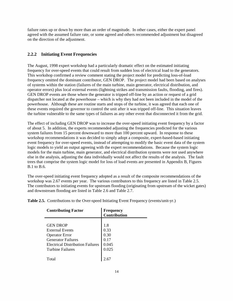
2.2.2 Initiating Event Frequencies The August, 1998 expert workshop had a particularly dramatic effect on the estimated initiating frequency for over-speed events that could result from sudden loss of electrical load to the generators. This workshop confirmed a review comment stating the project model for predicting loss-of-load frequency omitted the dominant contributor, GEN DROP. The project model had been based on analyses of systems within the station (failures of the main turbine, main generator, electrical distribution, and operator errors) plus local external events (lightning strikes and transmission faults, flooding, and fires). GEN DROP events are those where the generator is tripped off-line by an action or request of a grid dispatcher not located at the powerhouse – which is why they had not been included in the model of the powerhouse. Although these are routine starts and stops of the turbine, it was agreed that each one of these events required the governor to control the unit after it was tripped off-line. This situation leaves the turbine vulnerable to the same types of failures as any other event that disconnected it from the grid. The effect of including GEN DROP was to increase the over-speed initiating event frequency by a factor of about 5. In addition, the experts recommended adjusting the frequencies predicted for the various system failures from 15 percent downward to more than 100 percent upward. In response to these workshop recommendations it was decided to simply adopt a composite, expert-based-based initiating event frequency for over-speed events, instead of attempting to modify the basic event data of the system logic models to yield an output agreeing with the expert recommendations. Because the system logic models for the main turbine, main generator, and electrical distribution systems were not used anywhere else in the analysis, adjusting the data individually would not affect the results of the analysis. The fault trees that comprise the system logic model for loss of load events are presented in Appendix B, Figures B.1 to B.6. The over-speed initiating event frequency adopted as a result of the composite recommendations of the workshop was 2.67 events per year. The various contributors to this frequency are listed in Table 2.5. The contributors to initiating events for upstream flooding (originating from upstream of the wicket gates) and downstream flooding are listed in Table 2.6 and Table 2.7. Table 2.5. Contributions to the Over-speed Initiating Event Frequency (events/unit-yr.)

Contributing Factor Frequency Contribution

GEN DROP 1.8 External Events 0.33 Operator Error 0.30 Generator Failures 0.17 Electrical Distribution Failures 0.045 Turbine Failures 0.025 Total 2.67

15

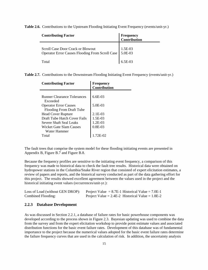
Table 2.6. Contributions to the Upstream Flooding Initiating Event Frequency (events/unit-yr.)

Contributing Factor Frequency Contribution

Scroll Case Door Crack or Blowout 1.5E-03 Operator Error Causes Flooding From Scroll Case 5.0E-03 Total 6.5E-03

Table 2.7. Contributions to the Downstream Flooding Initiating Event Frequency (events/unit-yr.)

Contributing Factor Frequency Contribution

Runner Clearance Tolerances 6.6E-03 Exceeded Operator Error Causes 5.0E-03 Flooding From Draft Tube Head Cover Rupture 2.1E-03 Draft Tube Hatch Cover Fails 1.5E-03 Severe Shaft Seal Leaks 1.2E-03 Wicket Gate Slam Causes 0.8E-03 Water Hammer Total 1.72E-02

The fault trees that comprise the system model for these flooding initiating events are presented in Appendix B, Figure B.7 and Figure B.8. Because the frequency profiles are sensitive to the initiating event frequency, a comparison of this frequency was made to historical data to check the fault tree results. Historical data were obtained on hydropower stations in the Columbia/Snake River region that consisted of expert elicitation estimates, a review of papers and reports, and the historical survey conducted as part of the data gathering effort for this project. The results showed excellent agreement between the values used in the project and the historical initiating event values (occurrences/unit-yr.): Loss of Load (without GEN DROP): Project Value = 8.7E-1 Historical Value = 7.0E-1 Combined Flooding: Project Value = 2.4E-2 Historical Value = 1.8E-2

2.2.3 Database Development As was discussed in Section 2.2.1, a database of failure rates for basic powerhouse components was developed according to the process shown in Figure 2.3. Bayesian updating was used to combine the data from the survey and from the expert elicitation workshop to provide point estimate values and associated distribution functions for the basic event failure rates. Development of this database was of fundamental importance to the project because the numerical values adopted for the basic event failure rates determine the failure frequency curves that are used in the calculation of risk. In addition, the uncertainty analysis

16

requires use of the distribution functions for each of the basic event failure rates in computing the uncertainty of the overall risk values. The survey data provide numbers of failures during a period of time for the components. This information was converted into number of failures (N) per operating unit-year (T) for each powerhouse by considering historical information on the hours of operation each year. For components not operating continuously (such as the gantry crane used to lower intake gates when required) failure rates were later converted to failure probability per demand. This computation was accomplished by dividing the failure rate per unit year by the demand rate (number of demands per unit year). The analysis assumed random and independent failures, and the failure process is described by a constant (but unknown) failure rate λ = N/T having a Poisson distribution. The conjugate distribution describing the probability that λ has a particular value, given that N failures are observed in time T, is a gamma function

p(λ) = γ(λ;β1, β2) (2.4)

where

β1 = N+1, and β2 = T. (2.5) Gamma functions having these properties were fitted to the survey data for each of the survey basic events addressed. Early in the project, an attempt was made to use a censored data approach to treat the survey data, because zero failures were reported for many of the components. The censoring approach ignores reports of zero failures, and develops failure rates from reports of failures that actually happened during the reporting time interval. However, the censored data approach requires time-to-failure data for individual components, that are not provided in the survey data; survey data only provide total failures in total operating time. Consequently, the censored data approach was abandoned in favor of the standard treatment of the data that is described previously and in the following discussions of Bayesian updating. The expert elicitation process described in Section 2.2.1 was used to obtain estimates of failure rates for each of the components addressed in the survey from each of the 11 experts at the December 1994 workshop. These estimates included the point estimate value of the failure probability, the upper and lower confidence bounds, and the rationale for the estimates. For each component, the raw data provided by the experts were fitted to a gamma distribution function having the same values of mean (M) and variance (V – the square of the standard deviation of the estimated values) as the mean and the variance of the expert estimations. Consequently, for each component, the probability that λ has any value is given by the function p(λ) = γ(λ;b1, b2) (2.6)

where b1 = M2/V, and b2 = M/V. (2.7) Bayesian analysis is a systematic method for combining failure data from multiple sources to create a single composite estimate (Lewis 1987; NRC 1981). The Bayesian formula stems from the fact that the intersection of two probabilities can be written in terms of two different conditional probabilities. For each component, the Bayesian approach was used to combine the failure rate distribution determined by the survey data with the failure rate distribution derived from the expert estimates to produce a final,

17

combined component failure rate distribution. This combined distribution is the product of the two gamma functions, and has the parameters p(λ) = γ(λ : N+b1, T+b2). (2.8)

The results of the Bayesian analysis are mean and median values of failure rates, and the parameters of the gamma distribution functions representing the uncertainty of these failure rates. Appendix A presents these results, along with the results of elicitations for components not addressed in the survey.

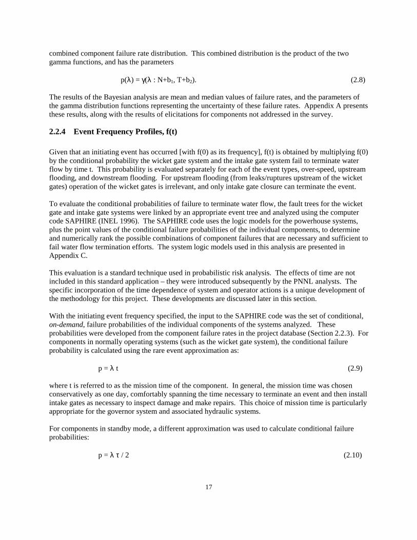
2.2.4 Event Frequency Profiles, f(t) Given that an initiating event has occurred [with f(0) as its frequency], f(t) is obtained by multiplying f(0) by the conditional probability the wicket gate system and the intake gate system fail to terminate water flow by time t. This probability is evaluated separately for each of the event types, over-speed, upstream flooding, and downstream flooding. For upstream flooding (from leaks/ruptures upstream of the wicket gates) operation of the wicket gates is irrelevant, and only intake gate closure can terminate the event. To evaluate the conditional probabilities of failure to terminate water flow, the fault trees for the wicket gate and intake gate systems were linked by an appropriate event tree and analyzed using the computer code SAPHIRE (INEL 1996). The SAPHIRE code uses the logic models for the powerhouse systems, plus the point values of the conditional failure probabilities of the individual components, to determine and numerically rank the possible combinations of component failures that are necessary and sufficient to fail water flow termination efforts. The system logic models used in this analysis are presented in Appendix C. This evaluation is a standard technique used in probabilistic risk analysis. The effects of time are not included in this standard application – they were introduced subsequently by the PNNL analysts. The specific incorporation of the time dependence of system and operator actions is a unique development of the methodology for this project. These developments are discussed later in this section. With the initiating event frequency specified, the input to the SAPHIRE code was the set of conditional, on-demand, failure probabilities of the individual components of the systems analyzed. These probabilities were developed from the component failure rates in the project database (Section 2.2.3). For components in normally operating systems (such as the wicket gate system), the conditional failure probability is calculated using the rare event approximation as:

p = λ t (2.9) where t is referred to as the mission time of the component. In general, the mission time was chosen conservatively as one day, comfortably spanning the time necessary to terminate an event and then install intake gates as necessary to inspect damage and make repairs. This choice of mission time is particularly appropriate for the governor system and associated hydraulic systems. For components in standby mode, a different approximation was used to calculate conditional failure probabilities: p = λ τ / 2 (2.10)

18

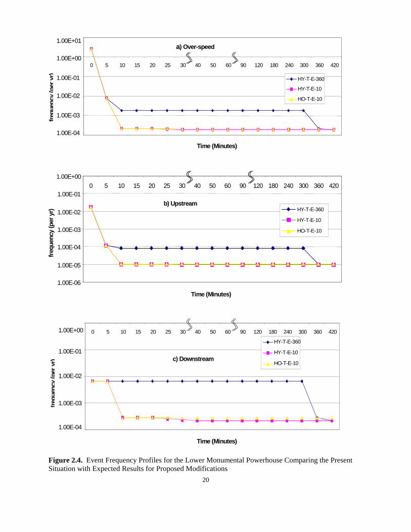
where τ is the time between tests or between operations that demonstrate operability. τ is often referred to as the fault exposure time of the component. Equation (2.10) captures the idea that τ/2 is the average time during the exposure for such damage to occur. In the wicket gate system, despite the fact that it is in continuous operation, complete closure of the wicket gates to shut down the unit occurs infrequently. Because of this infrequent operation, damage to the shift ring or servomotors that could prevent complete closure of the wicket gates might occur and remain unnoticed until a loss-of-load event required their rapid and complete closure. Consequently, for such components τ was chosen conservatively as half a year, because full operation of the system is demanded roughly twice a year. This situation also applies to intake gate system components. The database listings in Appendix A specify the values of τ and t that were used to convert failure rates to conditional, on-demand failure probabilities. The combinations of individual component failures that can fail the system function number in the thousands and are referred to as minimum cut sets. The conditional probability of failure of the system functions is the sum of the cut set failure probabilities. Each cut set failure probability is the product of the individual component failure probabilities (assuming they are independent). The SAPHIRE code generates the minimal cut sets, analyzes them, and ignores those with failure probability values less than a specified cut off value. The use of a cut-off value reduces time wasted in calculating tiny probabilities too small to affect the sum. PNNL analysts wrote a computer code using the Visual Basic Macro language in Microsoft Access software to explicitly incorporate into the cut sets the time dependence of system and operator actions. First, the cut sets were expanded to include the effects of potential operator action that would recover the functions of failed components. This expansion was accomplished by inserting time dependent recovery factors into the cut sets. Prior to operator action, the value of each recovery factor is 1.0; afterwards, its value is the probability of failure estimated for the recovery action. Thus, the effect of each recovery factor is to reduce the cut set failure probability to a fraction of its value preceding the operator action. The inclusion of recovery factors in cut sets is a standard technique in risk analysis. The unique aspect of this analysis is the incorporation of explicit timing information for each individual component actuation and for each separate operator recovery action. At every time step of the calculation, each basic event in each cut set was checked to see if it was activated. If none of the events were activated, the cut set was ignored, as none of the events could perform the system function. Thus, for example, the values of f(t) remain equal to f(0) for upstream flooding until the actuation of intake gates, because actuation of the wicket gates cannot affect flooding from locations upstream of the gates. If any of the basic events in a cut set were activated, the cut set was not ignored. The failure probability value for the activated event was used, and the failure probability values for basic events not activated were set equal to 1.0. Thus, immediately after wicket gate actuation f(0) was reduced by a factor equal to the sum of the probabilities of ways the wicket gate system could fail. At later times, recovery factors further reduced that sum, and eventually intake gate actuation added basic event factors from the intake gate system to the cut sets. Addition of basic event factors reduced the sum even further. Frequency profiles that compare the frequency effects of various important features of the designs are presented in Figure 2.4 and Figure 2.5. Figure 2.4 compares the frequency profiles for the proposed modifications to the Lower Monumental powerhouse with those for the present situation (compares HY-T-E-10 and HO-T-E-10 with HY-T-E-360). Parts a, b, and c of the figure present the comparison for over-speed, downstream flooding, and upstream flooding. All three parts of the figure yield the same conclusions: both modifications are clearly superior to the present situation; the hydraulic modification is slightly more reliable than the hoist modification. This conclusion is in complete agreement with the risk

19

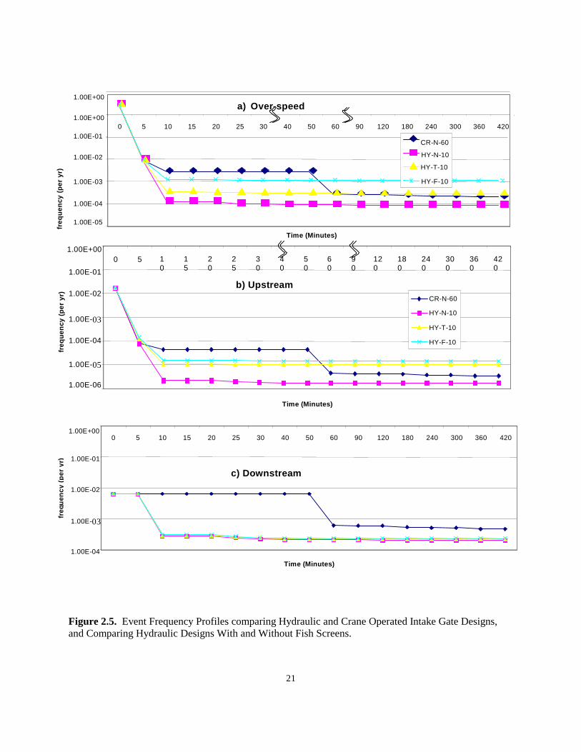
values tabulated in this section for the small powerhouse model that represents the Lower Monumental powerhouse. A similar situation is found (but not plotted here) when the frequency profiles for the proposed modifications to the McNary powerhouse (large model) and to the Little Goose/Lower Granite powerhouses (small model) are compared with the frequency profile for the present situation (compares HY-F-E-10 and HO-F-E-10 with HY-F-E-360). As was found for the Lower Monumental powerhouse, over-speed, upstream, and downstream flooding profiles yield the same conclusions: both modifications are clearly superior to the present situation, and the hydraulic modification is slightly more reliable than the hoist modification. This result agrees completely with the risk trends tabulated later in this section for the small and large powerhouse models. Figure 2.5 compares frequency profiles for different fish screen situations, and between hydraulic- and crane-operated intake gate systems. Frequency profiles are presented for HY-N-10, HY-T-10, HY-F-10 and CR-N-60. (Note the expected situation for crane-operated intake gates requires the crane be moved to the affected unit. This move will require 60 minutes for gate installation, as opposed to the optimum 30 minutes when the crane is situated at the unit). For the hydraulic systems, reliability is greatest for the design without fish screens, with traveling mesh screens yielding higher reliability than fixed bar screens. The crane system is significantly less reliable than the hydraulic systems due to the time required for intake gate installation. Once again, these results agree completely with the risk trends presented in this section. As was discussed briefly in Section 2.1, an uncertainty analysis was performed using a Monte Carlo approach with Latin Hypercube sampling of the data distribution functions. Section 2.2.3 describes the development of failure rate point estimates and distribution functions using a combination of survey data and estimates from an expert panel. The uncertainty analysis was performed using sampling from the distribution functions for the component data. Although the uncertainty analysis was performed primarily to bound the uncertainties of the final results of the analysis, information was developed for each step of the analysis process. Figure 2.6 presents the 5 percent and 95 percent uncertainty bounds, along with the point estimate values, of the frequency profiles for design HY-T-E-10. Parts a, b, and c present the results for over-speed, downstream, and upstream flooding. The overall uncertainty spread is about two orders of magnitude. The point estimate values are closer to the 95th percentile, as they are derived from mean values of the distributions, and therefore are larger than the results obtained using median values. These uncertainty results parallel the overall project results.

20

Figure 2.4. Event Frequency Profiles for the Lower Monumental Powerhouse Comparing the Present Situation with Expected Results for Proposed Modifications

a) Over-speed

1.00E-04

1.00E-03

1.00E-02

1.00E-01

1.00E+00

1.00E+01

0 5 10 15 20 25 30 40 50 60 90 120 180 240 300 360 420

Time (Minutes)

freq

uenc

y(p

eryr

)

HY-T-E-360

HY-T-E-10

HO-T-E-10

b) Upstream

1.00E-06

1.00E-05

1.00E-04

1.00E-03

1.00E-02

1.00E-01

1.00E+00 0 5 10 15 20 25 30 40 50 60 90 120 180 240 300 360 420

Time (Minutes)

freq

uenc

y (p

er y

r)

HY-T-E-360

HY-T-E-10

HO-T-E-10

c) Downstream

1.00E-04

1.00E-03

1.00E-02

1.00E-01

1.00E+00 0 5 10 15 20 25 30 40 50 60 90 120 180 240 300 360 420

Time (Minutes)

f req

uenc

y(p

eryr

)

HY-T-E-360

HY-T-E-10

HO-T-E-10

21

Figure 2.5. Event Frequency Profiles comparing Hydraulic and Crane Operated Intake Gate Designs, and Comparing Hydraulic Designs With and Without Fish Screens.

a) Over-speed

1.00E-05

1.00E-04

1.00E-03

1.00E-02

1.00E-01

1.00E+00

1.00E+00

0 5 10 15 20 25 30 40 50 60 90 120 180 240 300 360 420

Time (Minutes)

freq

uen

cy (

per

yr)

CR-N-60 HY-N-10 HY-T-10

HY-F-10

b) Upstream

1.00E-06

1.00E-05

1.00E-04

1.00E-03

1.00E-02

1.00E-01

1.00E+00 0 5 1

0 1 5

2 0

2 5

3 0

4 0

5 0

6 0

9 0

12 0

18 0

24 0

30 0

36 0

42 0

Time (Minutes)

freq

uen

cy (

per

yr)

CR-N-60

HY-N-10

HY-T-10

HY-F-10

c) Downstream

1.00E-04

1.00E-03

1.00E-02

1.00E-01

1.00E+00 0 5 10 15 20 25 30 40 50 60 90 120 180 240 300 360 420

Time (Minutes)

freq

uen

cy (

per

yr)

22

Figure 2.6. Uncertainty Bounds and Point Estimates for the Frequency Profiles for Design HY-T-E-10.

b) Upstream

1.00E-08

1.00E-07

1.00E-06

1.00E-05

1.00E-04

1.00E-03

1.00E-02

1.00E-01

1.00E+00

0 5 10 15 20 25 30 40 50 60 90 120 180 240 300 360 420

Time (minutes)

freq

uen

cy (

per

yr)

95th Percentile

HY-T-E-10

5th Percentile

a) Overspeed

1.00E-06

1.00E-05

1.00E-04

1.00E-03

1.00E-02

1.00E-01

1.00E+00

1.00E+01

0 5 10 15 20 25 30 40 50 60 90 120 180 240 300 360 420

Time (minutes)

freq

uen

cy (

per

yr)

95th Percentile

HY-T-E-10

5th Percentile

c) Downstream

1.00E-06

1.00E-05

1.00E-04

1.00E-03

1.00E-02

1.00E-01

1.00E+00

0 5 10 15 20 25 30 40 50 60 90 120 180 240 300 360 420

T im e (m in u te s )

fre

qu

en

cy (

pe

r yr

)

95th P erc ent ile

HY -T-E -10

5th P erc ent ile

23

2.3 Consequence Analysis At each time step, the project analysis estimated the economic consequences of over-speed, upstream, and downstream flooding events, initiated at time zero, that had progressed to the time under consideration. As shown in Figure 2.1 and Equation 2.3, these consequences were combined subsequently with the event frequencies at each time step, and summed over the event duration to determine the risk associated with each powerhouse design studied. Evaluation of the economic consequences requires the definition of potential damage states and their costs, and the estimation of the probability that each state represents the state of the powerhouse at each time step. Probabilities are estimated so they sum to unity at each time step of the analysis. This probabilistic analysis is used to allow analysis of a spectrum of potentially damaging situations of varying severity. (For instance, upstream flooding is assumed to result from either a crack or total blowout of the scroll case door, with equal likelihood.) This probabilistic analysis is discussed in Section 2.3.1. After the damage states are defined, the economic consequences of each powerhouse damage state must be estimated. Section 2.3.2 discusses the estimation of the various cost factors used in the calculation of total cost for each damage state. The four major cost categories considered are: construction costs to repair/replace/rebuild powerhouse equipment, environmental cleanup costs of oil spilled, lost income from the non-production of electricity, and interest costs for the money used to repair the damages.

2.3.1 Damage State Probabilities, D(t) The incorporation of explicit time dependence in the accident frequency analysis was required because damages from over-speed and flooding events increase with time after event initiation. Flooding damage increases as water rises through the powerhouse levels. Over-speed damage increases as bearings heat up and fail, turbine blades strike the speed ring and potentially break, the generator rotor contacts the stator and potentially damages windings and breaks off pole pieces, and shaft whip destroys the shaft packing and potentially damages the head cover. As these damages increase, flooding starts. This occurs through the head cover and shaft packing, and also through hatches into the scroll case and draft tube that would be affected by the vibrations and impacts accompanying the increasing mechanical damage. As is shown in Figure 2.1 and Equation 2.3, risk is calculated by combining the likelihood of an event lasting for a given time with the cost of the damage expected to accumulate during that time, summed over all time steps up to 8 hours after event initiation. In this section, the progression of damages during an event is analyzed without considering the likelihood of event termination. Once an event is initiated, it is treated as if it continues without mitigation for the entire 8-hour time span of the analysis. The likelihood of event mitigation or termination is addressed in the f(t) analysis. The damage state probabilities provide an estimate of what would happen as an event unfolds, and are used for subsequent combination with likelihood information through Equation 2.3.

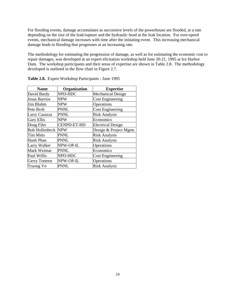
24

For flooding events, damage accumulates as successive levels of the powerhouse are flooded, at a rate depending on the size of the leak/rupture and the hydraulic head at the leak location. For over-speed events, mechanical damage increases with time after the initiating event. This increasing mechanical damage leads to flooding that progresses at an increasing rate. The methodology for estimating the progression of damage, as well as for estimating the economic cost to repair damages, was developed at an expert elicitation workshop held June 20-21, 1995 at Ice Harbor Dam. The workshop participants and their areas of expertise are shown in Table 2.8. The methodology developed is outlined in the flow chart in Figure 2.7. Table 2.8. Expert Workshop Participants - June 1995

Name Organization Expertise David Bardy NPD-HDC Mechanical Design Jesus Barrios NPW Cost Engineering Jim Bluhm NPW Operations Pete Broh PNNL Cost Engineering Larry Casazza PNNL Risk Analysis Gary Ellis NPW Economics Doug Filer CENPD-ET-HD Electrical Design Bob Hollenbeck NPW Design & Project Mgmt. Tim Mitts PNNL Risk Analysis Hanh Phan PNNL Risk Analysis Larry Walker NPW-OP-IL Operations Mark Weimar PNNL Economics Paul Willis NPD-HDC Cost Engineering Gerry Tomren NPW-OP-IL Operations Truong Vo PNNL Risk Analysis

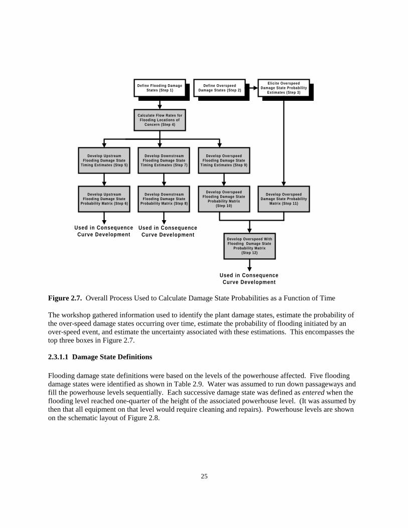
25

Figure 2.7. Overall Process Used to Calculate Damage State Probabilities as a Function of Time The workshop gathered information used to identify the plant damage states, estimate the probability of the over-speed damage states occurring over time, estimate the probability of flooding initiated by an over-speed event, and estimate the uncertainty associated with these estimations. This encompasses the top three boxes in Figure 2.7.

2.3.1.1 Damage State Definitions Flooding damage state definitions were based on the levels of the powerhouse affected. Five flooding damage states were identified as shown in Table 2.9. Water was assumed to run down passageways and fill the powerhouse levels sequentially. Each successive damage state was defined as entered when the flooding level reached one-quarter of the height of the associated powerhouse level. (It was assumed by then that all equipment on that level would require cleaning and repairs). Powerhouse levels are shown on the schematic layout of Figure 2.8.

Define Flooding DamageStates (Step 1)

Elicite OverspeedDamage State Probability

Estimates (Step 3)

Define OverspeedDamage States (Step 2)

Calculate Flow Rates forFlooding Locations of

Concern (Step 4)

Develop UpstreamFlooding Damage State

Timing Estimates (Step 5)

Develop DownstreamFlooding Damage State

Timing Estimates (Step 7)

Develop UpstreamFlooding Damage State

Probability Matrix (Step 6)

Develop DownstreamFlooding Damage State

Probability Matrix (Step 8)

Develop OverspeedFlooding Damage State

Timing Estimates (Step 9)

Develop OverspeedFlooding Damage State

Probability Matrix(Step 10)

Develop Overspeed WithFlooding Damage State

Probability Matrix(Step 12)

Used in ConsequenceCurve Development

Used in ConsequenceCurve Development

Used in ConsequenceCurve Development

Develop OverspeedDamage State Probability

Matrix (Step 11)

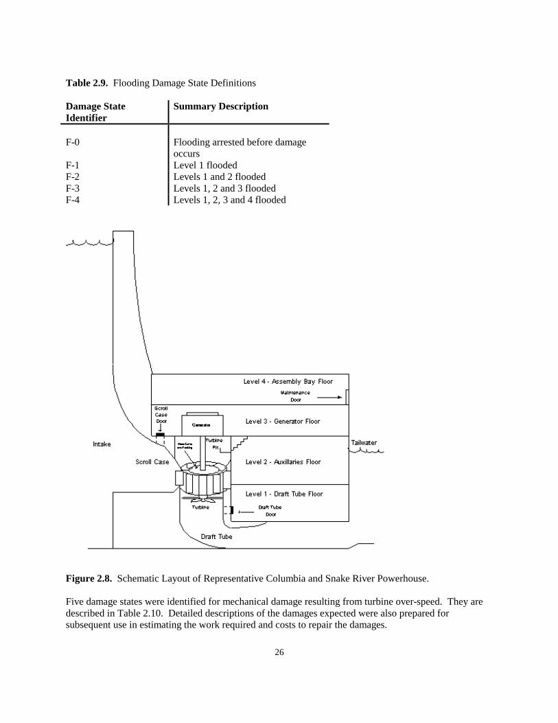
26

Table 2.9. Flooding Damage State Definitions Damage State Identifier

Summary Description

F-0 Flooding arrested before damage

occurs F-1 Level 1 flooded F-2 Levels 1 and 2 flooded F-3 Levels 1, 2 and 3 flooded F-4 Levels 1, 2, 3 and 4 flooded

Figure 2.8. Schematic Layout of Representative Columbia and Snake River Powerhouse. Five damage states were identified for mechanical damage resulting from turbine over-speed. They are described in Table 2.10. Detailed descriptions of the damages expected were also prepared for subsequent use in estimating the work required and costs to repair the damages.

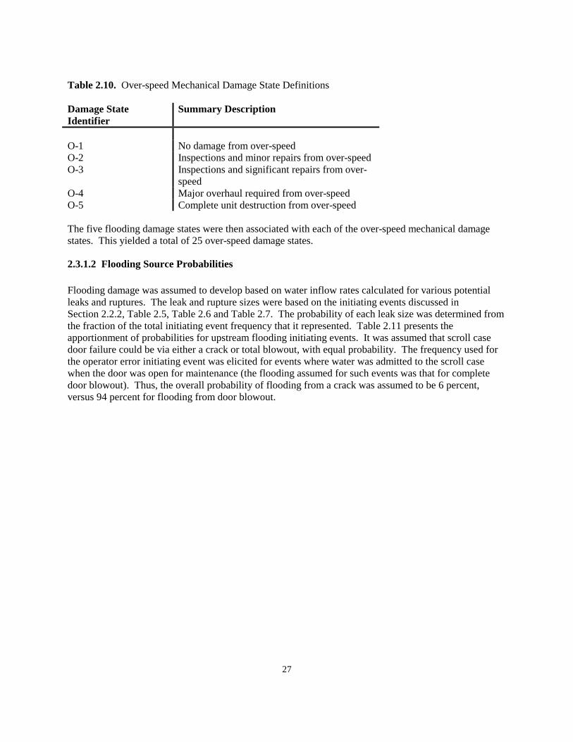
27

Table 2.10. Over-speed Mechanical Damage State Definitions Damage State Identifier

Summary Description

O-1 No damage from over-speed O-2 Inspections and minor repairs from over-speed O-3 Inspections and significant repairs from over-

speed O-4 Major overhaul required from over-speed O-5 Complete unit destruction from over-speed The five flooding damage states were then associated with each of the over-speed mechanical damage states. This yielded a total of 25 over-speed damage states.

2.3.1.2 Flooding Source Probabilities Flooding damage was assumed to develop based on water inflow rates calculated for various potential leaks and ruptures. The leak and rupture sizes were based on the initiating events discussed in Section 2.2.2, Table 2.5, Table 2.6 and Table 2.7. The probability of each leak size was determined from the fraction of the total initiating event frequency that it represented. Table 2.11 presents the apportionment of probabilities for upstream flooding initiating events. It was assumed that scroll case door failure could be via either a crack or total blowout, with equal probability. The frequency used for the operator error initiating event was elicited for events where water was admitted to the scroll case when the door was open for maintenance (the flooding assumed for such events was that for complete door blowout). Thus, the overall probability of flooding from a crack was assumed to be 6 percent, versus 94 percent for flooding from door blowout.

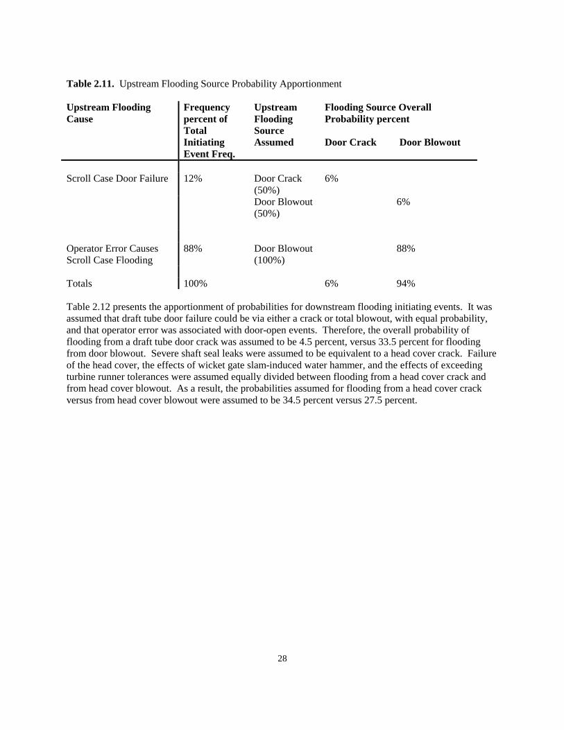
28

Table 2.11. Upstream Flooding Source Probability Apportionment Upstream Flooding Cause

Frequency percent of Total Initiating Event Freq.

Upstream Flooding Source Assumed

Flooding Source Overall Probability percent Door Crack Door Blowout

Door Crack (50%)

6% Scroll Case Door Failure

12%

Door Blowout (50%)

6%

Operator Error Causes Scroll Case Flooding

88% Door Blowout (100%)

88%

Totals 100% 6% 94% Table 2.12 presents the apportionment of probabilities for downstream flooding initiating events. It was assumed that draft tube door failure could be via either a crack or total blowout, with equal probability, and that operator error was associated with door-open events. Therefore, the overall probability of flooding from a draft tube door crack was assumed to be 4.5 percent, versus 33.5 percent for flooding from door blowout. Severe shaft seal leaks were assumed to be equivalent to a head cover crack. Failure of the head cover, the effects of wicket gate slam-induced water hammer, and the effects of exceeding turbine runner tolerances were assumed equally divided between flooding from a head cover crack and from head cover blowout. As a result, the probabilities assumed for flooding from a head cover crack versus from head cover blowout were assumed to be 34.5 percent versus 27.5 percent.

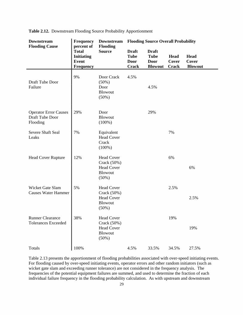
29

Table 2.12. Downstream Flooding Source Probability Apportionment Downstream Flooding Cause

Frequency percent of Total Initiating Event Frequency

Downstream Flooding Source

Flooding Source Overall Probability Draft Draft Tube Tube Head Head Door Door Cover Cover Crack Blowout Crack Blowout

Door Crack (50%)

4.5% Draft Tube Door Failure

9%

Door Blowout (50%)

4.5%

Operator Error Causes Draft Tube Door Flooding

29% Door Blowout (100%)

29%

Severe Shaft Seal Leaks

7% Equivalent Head Cover Crack (100%)

7%

Head Cover Crack (50%)

6% Head Cover Rupture 12%

Head Cover Blowout (50%)

6%

Head Cover Crack (50%)

2.5%

Wicket Gate Slam Causes Water Hammer

5%

Head Cover Blowout (50%)

2.5%

Runner Clearance Tolerances Exceeded

38% Head Cover Crack (50%)

19%

Head Cover Blowout (50%)

19%

Totals 100% 4.5% 33.5% 34.5% 27.5% Table 2.13 presents the apportionment of flooding probabilities associated with over-speed initiating events. For flooding caused by over-speed initiating events, operator errors and other random initiators (such as wicket gate slam and exceeding runner tolerance) are not considered in the frequency analysis. The frequencies of the potential equipment failures are summed, and used to determine the fraction of each individual failure frequency in the flooding probability calculation. As with upstream and downstream

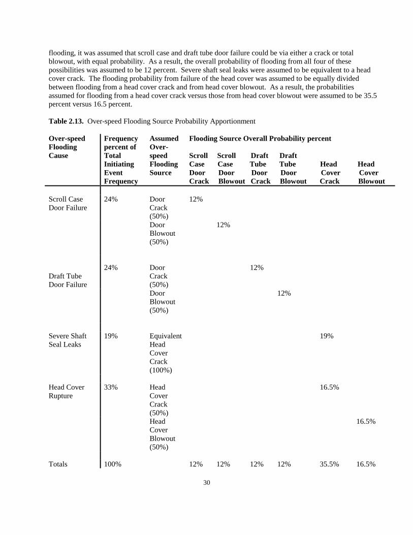
30

flooding, it was assumed that scroll case and draft tube door failure could be via either a crack or total blowout, with equal probability. As a result, the overall probability of flooding from all four of these possibilities was assumed to be 12 percent. Severe shaft seal leaks were assumed to be equivalent to a head cover crack. The flooding probability from failure of the head cover was assumed to be equally divided between flooding from a head cover crack and from head cover blowout. As a result, the probabilities assumed for flooding from a head cover crack versus those from head cover blowout were assumed to be 35.5 percent versus 16.5 percent. Table 2.13. Over-speed Flooding Source Probability Apportionment Over-speed Flooding Cause

Frequency percent of Total Initiating Event Frequency

Assumed Over-speed Flooding Source

Flooding Source Overall Probability percent Scroll Scroll Draft Draft Case Case Tube Tube Head Head Door Door Door Door Cover Cover Crack Blowout Crack Blowout Crack Blowout

Door Crack (50%)

12% Scroll Case Door Failure

24%

Door Blowout (50%)

12%

Door Crack (50%)

12% Draft Tube Door Failure

24%

Door Blowout (50%)

12%

Severe Shaft Seal Leaks

19% Equivalent Head Cover Crack (100%)

19%

Head Cover Crack (50%)

16.5% Head Cover Rupture

33%

Head Cover Blowout (50%)

16.5%

Totals 100% 12% 12% 12% 12% 35.5% 16.5%

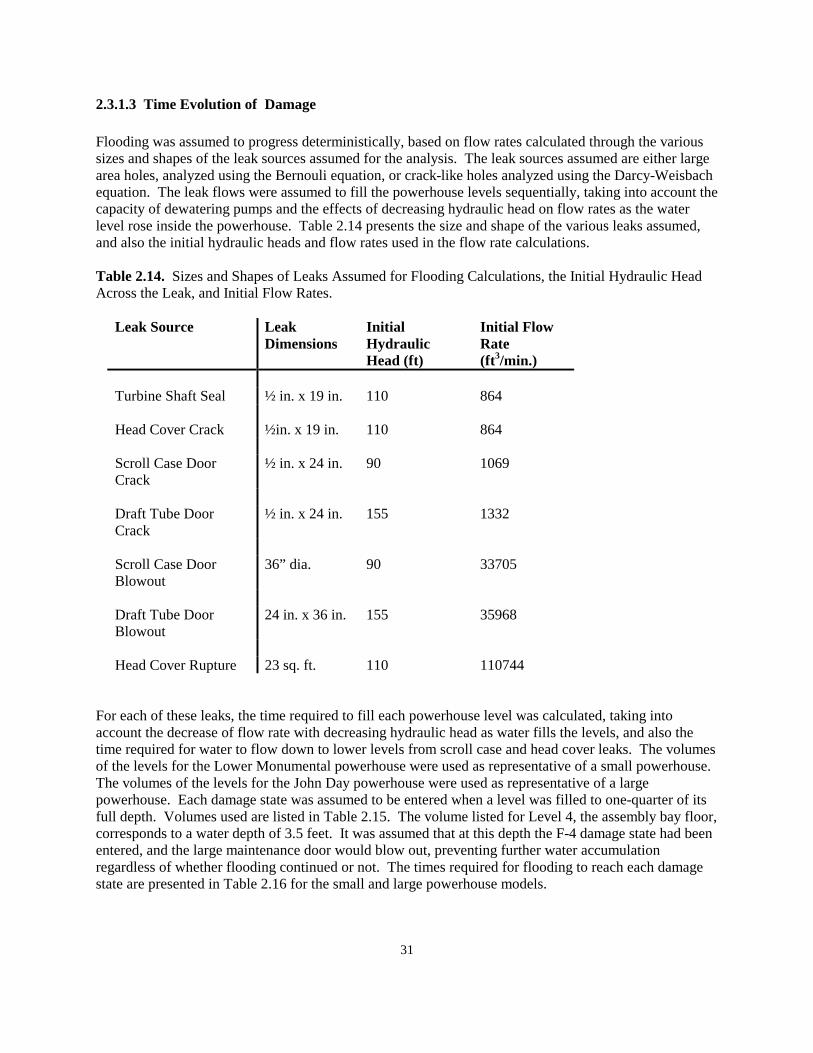
31

2.3.1.3 Time Evolution of Damage Flooding was assumed to progress deterministically, based on flow rates calculated through the various sizes and shapes of the leak sources assumed for the analysis. The leak sources assumed are either large area holes, analyzed using the Bernouli equation, or crack-like holes analyzed using the Darcy-Weisbach equation. The leak flows were assumed to fill the powerhouse levels sequentially, taking into account the capacity of dewatering pumps and the effects of decreasing hydraulic head on flow rates as the water level rose inside the powerhouse. Table 2.14 presents the size and shape of the various leaks assumed, and also the initial hydraulic heads and flow rates used in the flow rate calculations. Table 2.14. Sizes and Shapes of Leaks Assumed for Flooding Calculations, the Initial Hydraulic Head Across the Leak, and Initial Flow Rates.

Leak Source Leak Dimensions

Initial Hydraulic Head (ft)

Initial Flow Rate (ft3/min.)

Turbine Shaft Seal ½ in. x 19 in. 110 864 Head Cover Crack ½in. x 19 in. 110 864 Scroll Case Door Crack

½ in. x 24 in. 90 1069

Draft Tube Door Crack

½ in. x 24 in. 155 1332

Scroll Case Door Blowout

36” dia. 90 33705

Draft Tube Door Blowout

24 in. x 36 in. 155 35968

Head Cover Rupture 23 sq. ft. 110 110744

For each of these leaks, the time required to fill each powerhouse level was calculated, taking into account the decrease of flow rate with decreasing hydraulic head as water fills the levels, and also the time required for water to flow down to lower levels from scroll case and head cover leaks. The volumes of the levels for the Lower Monumental powerhouse were used as representative of a small powerhouse. The volumes of the levels for the John Day powerhouse were used as representative of a large powerhouse. Each damage state was assumed to be entered when a level was filled to one-quarter of its full depth. Volumes used are listed in Table 2.15. The volume listed for Level 4, the assembly bay floor, corresponds to a water depth of 3.5 feet. It was assumed that at this depth the F-4 damage state had been entered, and the large maintenance door would blow out, preventing further water accumulation regardless of whether flooding continued or not. The times required for flooding to reach each damage state are presented in Table 2.16 for the small and large powerhouse models.

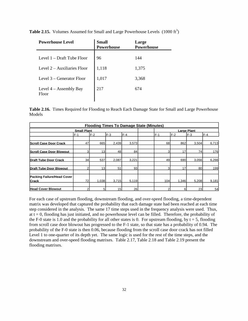
32

Table 2.15. Volumes Assumed for Small and Large Powerhouse Levels (1000 ft3)

Powerhouse Level Small Powerhouse

Large Powerhouse

Level 1 – Draft Tube Floor 96 144 Level 2 – Auxiliaries Floor 1,118 1,375 Level 3 – Generator Floor 1,017 3,368 Level 4 – Assembly Bay Floor

217 674

Table 2.16. Times Required for Flooding to Reach Each Damage State for Small and Large Powerhouse Models

Flooding Times To Damage State (Minutes)Small Plant Large PlantF-1 F-2 F-3 F-4 F-1 F-2 F-3 F-4

Scroll Case Door Crack 47 665 2,439 3,573 68 862 3,504 6,713

Scroll Case Door Blowout 3 13 48 84 3 17 74 176

Draft Tube Door Crack 34 537 2,087 3,221 49 690 3,056 6,266

Draft Tube Door Blowout 2 13 51 93 3 17 80 199

Packing Failure/Head Cover Crack 72 1,038 3,715 5,119 104 1,346 5,208 9,181

Head Cover Blowout 2 5 15 26 2 6 23 54 For each case of upstream flooding, downstream flooding, and over-speed flooding, a time-dependent matrix was developed that captured the probability that each damage state had been reached at each time step considered in the analysis. The same 17 time steps used in the frequency analysis were used. Thus, at t = 0, flooding has just initiated, and no powerhouse level can be filled. Therefore, the probability of the F-0 state is 1.0 and the probability for all other states is 0. For upstream flooding, by t = 5, flooding from scroll case door blowout has progressed to the F-1 state, so that state has a probability of 0.94. The probability of the F-0 state is then 0.06, because flooding from the scroll case door crack has not filled Level 1 to one-quarter of its depth yet. The same logic is used for the rest of the time steps, and the downstream and over-speed flooding matrixes. Table 2.17, Table 2.18 and Table 2.19 present the flooding matrixes.

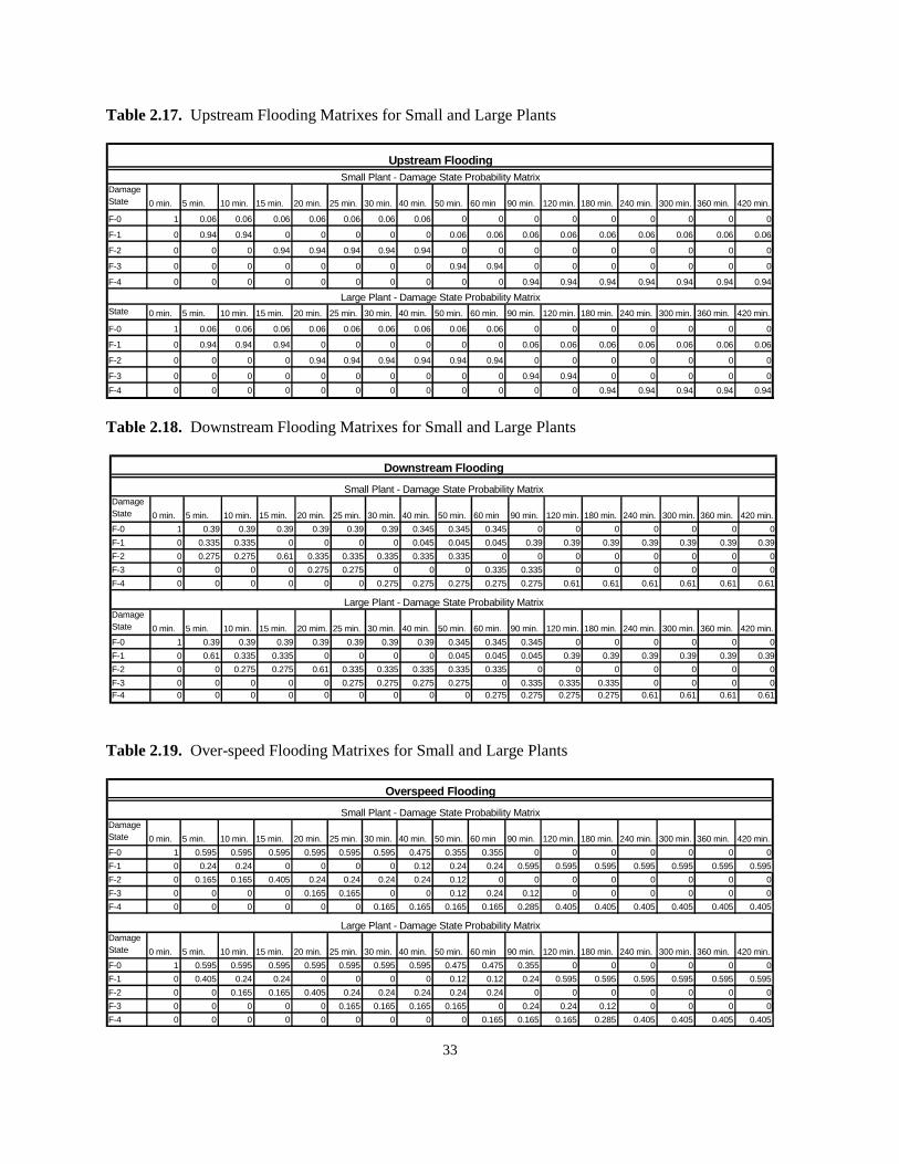
33

Table 2.17. Upstream Flooding Matrixes for Small and Large Plants

Table 2.18. Downstream Flooding Matrixes for Small and Large Plants

Table 2.19. Over-speed Flooding Matrixes for Small and Large Plants

Damage State 0 min. 5 min. 10 min. 15 min. 20 min. 25 min. 30 min. 40 min. 50 min. 60 min 90 min. 120 min. 180 min. 240 min. 300 min. 360 min. 420 min.

F-0 1 0.06 0.06 0.06 0.06 0.06 0.06 0.06 0 0 0 0 0 0 0 0 0

F-1 0 0.94 0.94 0 0 0 0 0 0.06 0.06 0.06 0.06 0.06 0.06 0.06 0.06 0.06

F-2 0 0 0 0.94 0.94 0.94 0.94 0.94 0 0 0 0 0 0 0 0 0

F-3 0 0 0 0 0 0 0 0 0.94 0.94 0 0 0 0 0 0 0

F-4 0 0 0 0 0 0 0 0 0 0 0.94 0.94 0.94 0.94 0.94 0.94 0.94

State 0 min. 5 min. 10 min. 15 min. 20 min. 25 min. 30 min. 40 min. 50 min. 60 min. 90 min. 120 min. 180 min. 240 min. 300 min. 360 min. 420 min.

F-0 1 0.06 0.06 0.06 0.06 0.06 0.06 0.06 0.06 0.06 0 0 0 0 0 0 0

F-1 0 0.94 0.94 0.94 0 0 0 0 0 0 0.06 0.06 0.06 0.06 0.06 0.06 0.06

F-2 0 0 0 0 0.94 0.94 0.94 0.94 0.94 0.94 0 0 0 0 0 0 0

F-3 0 0 0 0 0 0 0 0 0 0 0.94 0.94 0 0 0 0 0

F-4 0 0 0 0 0 0 0 0 0 0 0 0 0.94 0.94 0.94 0.94 0.94

Small Plant - Damage State Probability Matrix

Upstream Flooding

Large Plant - Damage State Probability Matrix

Damage State 0 min. 5 min. 10 min. 15 min. 20 min. 25 min. 30 min. 40 min. 50 min. 60 min 90 min. 120 min. 180 min. 240 min. 300 min. 360 min. 420 min.

F-0 1 0.595 0.595 0.595 0.595 0.595 0.595 0.475 0.355 0.355 0 0 0 0 0 0 0

F-1 0 0.24 0.24 0 0 0 0 0.12 0.24 0.24 0.595 0.595 0.595 0.595 0.595 0.595 0.595

F-2 0 0.165 0.165 0.405 0.24 0.24 0.24 0.24 0.12 0 0 0 0 0 0 0 0

F-3 0 0 0 0 0.165 0.165 0 0 0.12 0.24 0.12 0 0 0 0 0 0

F-4 0 0 0 0 0 0 0.165 0.165 0.165 0.165 0.285 0.405 0.405 0.405 0.405 0.405 0.405

Damage State 0 min. 5 min. 10 min. 15 min. 20 min. 25 min. 30 min. 40 min. 50 min. 60 min 90 min. 120 min. 180 min. 240 min. 300 min. 360 min. 420 min.

F-0 1 0.595 0.595 0.595 0.595 0.595 0.595 0.595 0.475 0.475 0.355 0 0 0 0 0 0

F-1 0 0.405 0.24 0.24 0 0 0 0 0.12 0.12 0.24 0.595 0.595 0.595 0.595 0.595 0.595

F-2 0 0 0.165 0.165 0.405 0.24 0.24 0.24 0.24 0.24 0 0 0 0 0 0 0

F-3 0 0 0 0 0 0.165 0.165 0.165 0.165 0 0.24 0.24 0.12 0 0 0 0

F-4 0 0 0 0 0 0 0 0 0 0.165 0.165 0.165 0.285 0.405 0.405 0.405 0.405

Overspeed Flooding

Small Plant - Damage State Probability Matrix

Large Plant - Damage State Probability Matrix

Damage State 0 min. 5 min. 10 min. 15 min. 20 min. 25 min. 30 min. 40 min. 50 min. 60 min 90 min. 120 min. 180 min. 240 min. 300 min. 360 min. 420 min.

F-0 1 0.39 0.39 0.39 0.39 0.39 0.39 0.345 0.345 0.345 0 0 0 0 0 0 0

F-1 0 0.335 0.335 0 0 0 0 0.045 0.045 0.045 0.39 0.39 0.39 0.39 0.39 0.39 0.39

F-2 0 0.275 0.275 0.61 0.335 0.335 0.335 0.335 0.335 0 0 0 0 0 0 0 0

F-3 0 0 0 0 0.275 0.275 0 0 0 0.335 0.335 0 0 0 0 0 0

F-4 0 0 0 0 0 0 0.275 0.275 0.275 0.275 0.275 0.61 0.61 0.61 0.61 0.61 0.61

Damage State 0 min. 5 min. 10 min. 15 min. 20 mim. 25 min. 30 min. 40 min. 50 min. 60 min. 90 min. 120 min. 180 min. 240 min. 300 min. 360 min. 420 min.

F-0 1 0.39 0.39 0.39 0.39 0.39 0.39 0.39 0.345 0.345 0.345 0 0 0 0 0 0

F-1 0 0.61 0.335 0.335 0 0 0 0 0.045 0.045 0.045 0.39 0.39 0.39 0.39 0.39 0.39

F-2 0 0 0.275 0.275 0.61 0.335 0.335 0.335 0.335 0.335 0 0 0 0 0 0 0

F-3 0 0 0 0 0 0.275 0.275 0.275 0.275 0 0.335 0.335 0.335 0 0 0 0F-4 0 0 0 0 0 0 0 0 0 0.275 0.275 0.275 0.275 0.61 0.61 0.61 0.61

Large Plant - Damage State Probability Matrix

Downstream Flooding

Small Plant - Damage State Probability Matrix

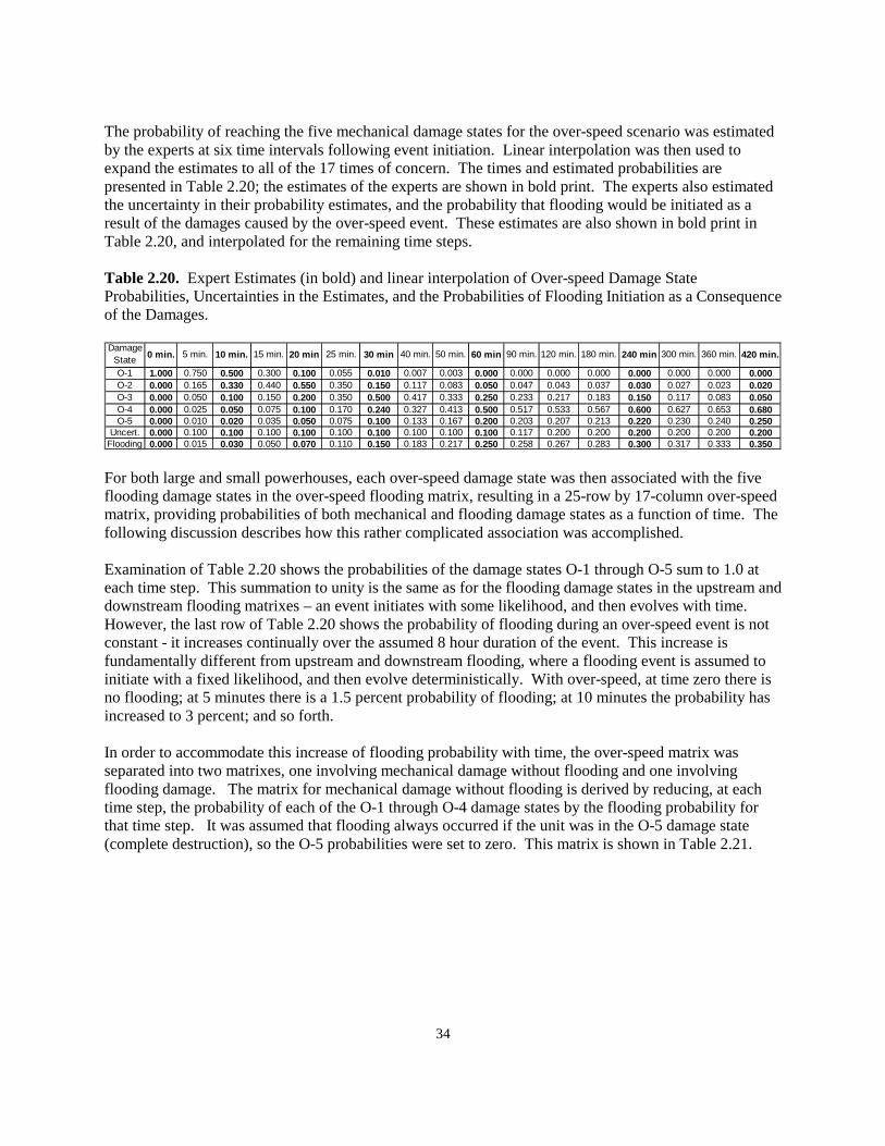
34

The probability of reaching the five mechanical damage states for the over-speed scenario was estimated by the experts at six time intervals following event initiation. Linear interpolation was then used to expand the estimates to all of the 17 times of concern. The times and estimated probabilities are presented in Table 2.20; the estimates of the experts are shown in bold print. The experts also estimated the uncertainty in their probability estimates, and the probability that flooding would be initiated as a result of the damages caused by the over-speed event. These estimates are also shown in bold print in Table 2.20, and interpolated for the remaining time steps. Table 2.20. Expert Estimates (in bold) and linear interpolation of Over-speed Damage State Probabilities, Uncertainties in the Estimates, and the Probabilities of Flooding Initiation as a Consequence of the Damages. Damage

State 0 min. 5 min. 10 min. 15 min. 20 min 25 min. 30 min 40 min. 50 min. 60 min 90 min. 120 min. 180 min. 240 min 300 min. 360 min. 420 min.

O-1 1.000 0.750 0.500 0.300 0.100 0.055 0.010 0.007 0.003 0.000 0.000 0.000 0.000 0.000 0.000 0.000 0.000O-2 0.000 0.165 0.330 0.440 0.550 0.350 0.150 0.117 0.083 0.050 0.047 0.043 0.037 0.030 0.027 0.023 0.020O-3 0.000 0.050 0.100 0.150 0.200 0.350 0.500 0.417 0.333 0.250 0.233 0.217 0.183 0.150 0.117 0.083 0.050O-4 0.000 0.025 0.050 0.075 0.100 0.170 0.240 0.327 0.413 0.500 0.517 0.533 0.567 0.600 0.627 0.653 0.680O-5 0.000 0.010 0.020 0.035 0.050 0.075 0.100 0.133 0.167 0.200 0.203 0.207 0.213 0.220 0.230 0.240 0.250

Uncert. 0.000 0.100 0.100 0.100 0.100 0.100 0.100 0.100 0.100 0.100 0.117 0.200 0.200 0.200 0.200 0.200 0.200Flooding 0.000 0.015 0.030 0.050 0.070 0.110 0.150 0.183 0.217 0.250 0.258 0.267 0.283 0.300 0.317 0.333 0.350 For both large and small powerhouses, each over-speed damage state was then associated with the five flooding damage states in the over-speed flooding matrix, resulting in a 25-row by 17-column over-speed matrix, providing probabilities of both mechanical and flooding damage states as a function of time. The following discussion describes how this rather complicated association was accomplished. Examination of Table 2.20 shows the probabilities of the damage states O-1 through O-5 sum to 1.0 at each time step. This summation to unity is the same as for the flooding damage states in the upstream and downstream flooding matrixes – an event initiates with some likelihood, and then evolves with time. However, the last row of Table 2.20 shows the probability of flooding during an over-speed event is not constant - it increases continually over the assumed 8 hour duration of the event. This increase is fundamentally different from upstream and downstream flooding, where a flooding event is assumed to initiate with a fixed likelihood, and then evolve deterministically. With over-speed, at time zero there is no flooding; at 5 minutes there is a 1.5 percent probability of flooding; at 10 minutes the probability has increased to 3 percent; and so forth. In order to accommodate this increase of flooding probability with time, the over-speed matrix was separated into two matrixes, one involving mechanical damage without flooding and one involving flooding damage. The matrix for mechanical damage without flooding is derived by reducing, at each time step, the probability of each of the O-1 through O-4 damage states by the flooding probability for that time step. It was assumed that flooding always occurred if the unit was in the O-5 damage state (complete destruction), so the O-5 probabilities were set to zero. This matrix is shown in Table 2.21.

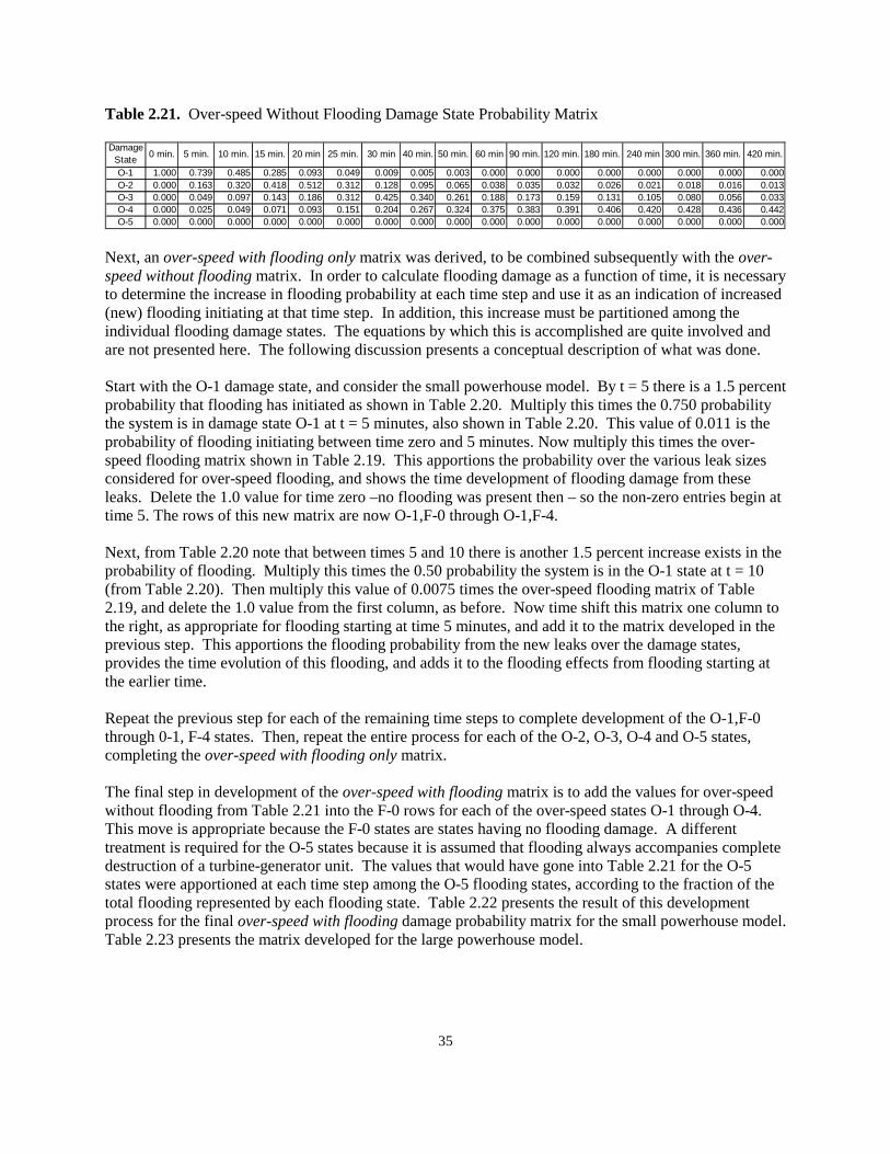
35

Table 2.21. Over-speed Without Flooding Damage State Probability Matrix Damage

State0 min. 5 min. 10 min. 15 min. 20 min 25 min. 30 min 40 min. 50 min. 60 min 90 min. 120 min. 180 min. 240 min 300 min. 360 min. 420 min.

O-1 1.000 0.739 0.485 0.285 0.093 0.049 0.009 0.005 0.003 0.000 0.000 0.000 0.000 0.000 0.000 0.000 0.000O-2 0.000 0.163 0.320 0.418 0.512 0.312 0.128 0.095 0.065 0.038 0.035 0.032 0.026 0.021 0.018 0.016 0.013O-3 0.000 0.049 0.097 0.143 0.186 0.312 0.425 0.340 0.261 0.188 0.173 0.159 0.131 0.105 0.080 0.056 0.033O-4 0.000 0.025 0.049 0.071 0.093 0.151 0.204 0.267 0.324 0.375 0.383 0.391 0.406 0.420 0.428 0.436 0.442O-5 0.000 0.000 0.000 0.000 0.000 0.000 0.000 0.000 0.000 0.000 0.000 0.000 0.000 0.000 0.000 0.000 0.000

Next, an over-speed with flooding only matrix was derived, to be combined subsequently with the over-speed without flooding matrix. In order to calculate flooding damage as a function of time, it is necessary to determine the increase in flooding probability at each time step and use it as an indication of increased (new) flooding initiating at that time step. In addition, this increase must be partitioned among the individual flooding damage states. The equations by which this is accomplished are quite involved and are not presented here. The following discussion presents a conceptual description of what was done. Start with the O-1 damage state, and consider the small powerhouse model. By t = 5 there is a 1.5 percent probability that flooding has initiated as shown in Table 2.20. Multiply this times the 0.750 probability the system is in damage state O-1 at t = 5 minutes, also shown in Table 2.20. This value of 0.011 is the probability of flooding initiating between time zero and 5 minutes. Now multiply this times the over-speed flooding matrix shown in Table 2.19. This apportions the probability over the various leak sizes considered for over-speed flooding, and shows the time development of flooding damage from these leaks. Delete the 1.0 value for time zero –no flooding was present then – so the non-zero entries begin at time 5. The rows of this new matrix are now O-1,F-0 through O-1,F-4. Next, from Table 2.20 note that between times 5 and 10 there is another 1.5 percent increase exists in the probability of flooding. Multiply this times the 0.50 probability the system is in the O-1 state at t = 10 (from Table 2.20). Then multiply this value of 0.0075 times the over-speed flooding matrix of Table 2.19, and delete the 1.0 value from the first column, as before. Now time shift this matrix one column to the right, as appropriate for flooding starting at time 5 minutes, and add it to the matrix developed in the previous step. This apportions the flooding probability from the new leaks over the damage states, provides the time evolution of this flooding, and adds it to the flooding effects from flooding starting at the earlier time. Repeat the previous step for each of the remaining time steps to complete development of the O-1,F-0 through 0-1, F-4 states. Then, repeat the entire process for each of the O-2, O-3, O-4 and O-5 states, completing the over-speed with flooding only matrix. The final step in development of the over-speed with flooding matrix is to add the values for over-speed without flooding from Table 2.21 into the F-0 rows for each of the over-speed states O-1 through O-4. This move is appropriate because the F-0 states are states having no flooding damage. A different treatment is required for the O-5 states because it is assumed that flooding always accompanies complete destruction of a turbine-generator unit. The values that would have gone into Table 2.21 for the O-5 states were apportioned at each time step among the O-5 flooding states, according to the fraction of the total flooding represented by each flooding state. Table 2.22 presents the result of this development process for the final over-speed with flooding damage probability matrix for the small powerhouse model. Table 2.23 presents the matrix developed for the large powerhouse model.

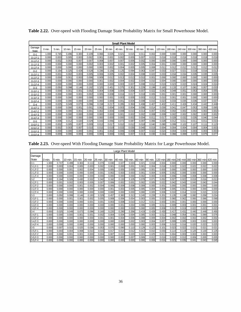
36

Table 2.22. Over-speed with Flooding Damage State Probability Matrix for Small Powerhouse Model.

Table 2.23. Over-speed With Flooding Damage State Probability Matrix for Large Powerhouse Model.

Small Plant ModelDamage

State0 min. 5 min. 10 min. 15 min. 20 min 25 min. 30 min 40 min. 50 min. 60 min 90 min. 120 min. 180 min. 240 min 300 min. 360 min. 420 min.

O-1 1.000 0.745 0.496 0.300 0.109 0.066 0.026 0.021 0.015 0.011 0.002 0.000 0.000 0.000 0.000 0.000 0.000

O-1,F-1 0.000 0.003 0.005 0.003 0.002 0.001 0.001 0.002 0.005 0.007 0.015 0.018 0.018 0.018 0.018 0.018 0.018

O-1,F-2 0.000 0.002 0.003 0.007 0.007 0.008 0.007 0.007 0.005 0.002 0.000 0.000 0.000 0.000 0.000 0.000 0.000

O-1,F-3 0.000 0.000 0.000 0.000 0.002 0.003 0.002 0.001 0.002 0.005 0.004 0.001 0.000 0.000 0.000 0.000 0.000

O-1,F-4 0.000 0.000 0.000 0.000 0.000 0.000 0.002 0.004 0.005 0.005 0.008 0.011 0.012 0.012 0.012 0.012 0.012

O-2 0.000 0.164 0.325 0.428 0.528 0.336 0.156 0.125 0.094 0.063 0.047 0.033 0.027 0.021 0.018 0.016 0.013

O-2,F-1 0.000 0.001 0.002 0.003 0.005 0.006 0.005 0.002 0.004 0.008 0.022 0.033 0.034 0.034 0.035 0.035 0.035

O-2,F-2 0.000 0.000 0.001 0.003 0.006 0.009 0.012 0.013 0.013 0.010 0.001 0.000 0.000 0.000 0.000 0.000 0.000

O-2,F-3 0.000 0.000 0.000 0.000 0.000 0.001 0.002 0.004 0.002 0.004 0.010 0.004 0.000 0.000 0.000 0.000 0.000

O-2,F-4 0.000 0.000 0.000 0.000 0.000 0.000 0.000 0.003 0.007 0.008 0.012 0.019 0.023 0.023 0.024 0.024 0.024

O-3 0.000 0.050 0.098 0.146 0.192 0.325 0.451 0.375 0.301 0.229 0.199 0.165 0.133 0.107 0.081 0.057 0.033

O-3,F-1 0.000 0.000 0.001 0.001 0.002 0.004 0.008 0.004 0.004 0.007 0.022 0.043 0.049 0.051 0.053 0.054 0.055

O-3,F-2 0.000 0.000 0.000 0.001 0.002 0.005 0.008 0.016 0.017 0.018 0.005 0.001 0.001 0.001 0.000 0.000 0.000

O-3,F-3 0.000 0.000 0.000 0.000 0.000 0.000 0.001 0.003 0.005 0.003 0.013 0.010 0.001 0.001 0.000 0.000 0.000

O-3,F-4 0.000 0.000 0.000 0.000 0.000 0.000 0.000 0.001 0.004 0.008 0.015 0.023 0.033 0.035 0.036 0.037 0.037

O-4 0.000 0.025 0.049 0.073 0.096 0.158 0.217 0.285 0.350 0.408 0.407 0.402 0.411 0.426 0.434 0.442 0.448

O-4,F-1 0.000 0.000 0.000 0.001 0.001 0.002 0.004 0.003 0.004 0.006 0.014 0.030 0.041 0.047 0.053 0.059 0.065

O-4,F-2 0.000 0.000 0.000 0.001 0.001 0.002 0.004 0.008 0.010 0.014 0.007 0.002 0.002 0.002 0.002 0.002 0.002

O-4,F-3 0.000 0.000 0.000 0.000 0.000 0.000 0.000 0.001 0.002 0.002 0.008 0.009 0.002 0.002 0.002 0.002 0.002

O-4,F-4 0.000 0.000 0.000 0.000 0.000 0.000 0.000 0.000 0.002 0.004 0.011 0.017 0.028 0.032 0.035 0.040 0.044

O-5 0.000 0.006 0.012 0.020 0.029 0.043 0.056 0.072 0.087 0.097 0.066 0.028 0.012 0.011 0.011 0.011 0.010

O-5,F-1 0.000 0.002 0.005 0.007 0.009 0.013 0.017 0.010 0.012 0.018 0.040 0.080 0.099 0.102 0.107 0.111 0.115

O-5,F-2 0.000 0.002 0.003 0.007 0.010 0.015 0.019 0.033 0.035 0.040 0.019 0.004 0.004 0.004 0.004 0.004 0.003

O-5,F-3 0.000 0.000 0.000 0.000 0.001 0.001 0.002 0.006 0.008 0.007 0.022 0.024 0.004 0.004 0.003 0.003 0.003

O-5,F-4 0.000 0.000 0.000 0.000 0.000 0.000 0.000 0.002 0.007 0.013 0.030 0.044 0.066 0.069 0.072 0.075 0.077

Damage State 0 min. 5 min. 10 min. 15 min. 20 min 25 min. 30 min 40 min. 50 min. 60 min 90 min. 120 min 180 min 240 min 300 min.360 min.420 min.O-1 1.000 0.747 0.499 0.303 0.113 0.070 0.030 0.027 0.024 0.021 0.018 0.004 0.000 0.000 0.000 0.000 0.000O-1,F-1 0.000 0.003 0.004 0.005 0.003 0.002 0.001 0.000 0.001 0.001 0.004 0.018 0.022 0.022 0.022 0.022 0.022O-1,F-2 0.000 0.000 0.001 0.002 0.004 0.005 0.005 0.005 0.005 0.005 0.001 0.000 0.000 0.000 0.000 0.000 0.000O-1,F-3 0.000 0.000 0.000 0.000 0.000 0.001 0.002 0.003 0.003 0.001 0.004 0.005 0.002 0.000 0.000 0.000 0.000O-1,F-4 0.000 0.000 0.000 0.000 0.000 0.000 0.000 0.000 0.000 0.002 0.003 0.003 0.006 0.008 0.008 0.008 0.008O-2 0.000 0.164 0.326 0.430 0.532 0.342 0.162 0.133 0.105 0.078 0.071 0.052 0.027 0.022 0.019 0.016 0.013O-2,F-1 0.000 0.001 0.002 0.003 0.005 0.007 0.006 0.002 0.001 0.002 0.005 0.022 0.042 0.043 0.043 0.043 0.044O-2,F-2 0.000 0.000 0.000 0.001 0.002 0.004 0.006 0.009 0.008 0.009 0.005 0.001 0.000 0.000 0.000 0.000 0.000O-2,F-3 0.000 0.000 0.000 0.000 0.000 0.000 0.001 0.003 0.005 0.005 0.004 0.009 0.005 0.001 0.000 0.000 0.000O-2,F-4 0.000 0.000 0.000 0.000 0.000 0.000 0.000 0.000 0.000 0.000 0.005 0.006 0.010 0.014 0.015 0.015 0.015O-3 0.000 0.050 0.099 0.146 0.193 0.329 0.457 0.383 0.313 0.245 0.228 0.201 0.135 0.108 0.082 0.058 0.034O-3,F-1 0.000 0.000 0.001 0.001 0.002 0.005 0.008 0.006 0.004 0.003 0.005 0.020 0.060 0.062 0.065 0.066 0.068O-3,F-2 0.000 0.000 0.000 0.000 0.001 0.001 0.003 0.008 0.010 0.012 0.011 0.003 0.001 0.001 0.000 0.000 0.000O-3,F-3 0.000 0.000 0.000 0.000 0.000 0.000 0.000 0.001 0.004 0.006 0.005 0.011 0.009 0.003 0.001 0.001 0.001O-3,F-4 0.000 0.000 0.000 0.000 0.000 0.000 0.000 0.000 0.000 0.000 0.005 0.008 0.012 0.019 0.022 0.023 0.023O-4 0.000 0.025 0.049 0.073 0.096 0.160 0.220 0.290 0.356 0.419 0.428 0.430 0.417 0.431 0.440 0.448 0.455O-4,F-1 0.000 0.000 0.000 0.001 0.001 0.002 0.004 0.004 0.004 0.005 0.003 0.012 0.048 0.054 0.061 0.069 0.076O-4,F-2 0.000 0.000 0.000 0.000 0.000 0.001 0.001 0.004 0.006 0.008 0.009 0.004 0.002 0.002 0.002 0.002 0.002O-4,F-3 0.000 0.000 0.000 0.000 0.000 0.000 0.000 0.000 0.002 0.003 0.004 0.007 0.009 0.005 0.003 0.003 0.003O-4,F-4 0.000 0.000 0.000 0.000 0.000 0.000 0.000 0.000 0.000 0.000 0.003 0.006 0.010 0.016 0.020 0.023 0.025O-5 0.000 0.007 0.015 0.025 0.036 0.053 0.070 0.090 0.110 0.129 0.123 0.101 0.023 0.022 0.021 0.021 0.021O-5,F-1 0.000 0.003 0.004 0.008 0.010 0.015 0.017 0.014 0.012 0.013 0.010 0.033 0.114 0.119 0.125 0.130 0.135O-5,F-2 0.000 0.000 0.001 0.001 0.003 0.004 0.007 0.016 0.020 0.024 0.025 0.011 0.004 0.003 0.003 0.003 0.003O-5,F-3 0.000 0.000 0.000 0.000 0.000 0.000 0.000 0.002 0.007 0.009 0.012 0.019 0.020 0.010 0.006 0.005 0.005O-5,F-4 0.000 0.000 0.000 0.000 0.000 0.000 0.000 0.000 0.000 0.000 0.008 0.016 0.023 0.035 0.041 0.043 0.045

Large Plant Model

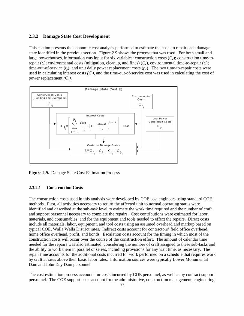
37

2.3.2 Damage State Cost Development This section presents the economic cost analysis performed to estimate the costs to repair each damage state identified in the previous section. Figure 2.9 shows the process that was used. For both small and large powerhouses, information was input for six variables: construction costs (Cc); construction time-to-repair (tr); environmental costs (mitigation, cleanup, and fines) (Ce), environmental time-to-repair (te); time-out-of-service (tp); and unit daily power replacement costs (pc). The two time-to-repair costs were used in calculating interest costs (CI), and the time-out-of-service cost was used in calculating the cost of power replacement (Cp).

Damage Sta te Cost (E)

Construct ion Costs(Flooding and Overspeed)

Envi ronmenta lCosts

Interest CostsLost Power

Generat ion Costs

Costs for Damage States

C ci C ei

C piC Ii

= 1

Pi

r

.Cost i

Pi

1Interest

12

k .5

Cost i

Ei

C ci

C ei

C Ii

C pi

Figure 2.9. Damage State Cost Estimation Process

2.3.2.1 Construction Costs The construction costs used in this analysis were developed by COE cost engineers using standard COE methods. First, all activities necessary to return the affected unit to normal operating status were identified and described at the sub-task level to estimate the work time required and the number of craft and support personnel necessary to complete the repairs. Cost contributions were estimated for labor, materials, and consumables, and for the equipment and tools needed to effect the repairs. Direct costs include all materials, labor, equipment, and tool costs using an assumed overhead and markup based on typical COE, Walla Walla District rates. Indirect costs account for contractors’ field office overhead, home office overhead, profit, and bonds. Escalation costs account for the timing in which most of the construction costs will occur over the course of the construction effort. The amount of calendar time needed for the repairs was also estimated, considering the number of craft assigned to these sub-tasks and the ability to work them in parallel or series, including provisions for any wait time, as necessary. The repair time accounts for the additional costs incurred for work performed on a schedule that requires work by craft at rates above their basic labor rates. Information sources were typically Lower Monumental Dam and John Day Dam personnel. The cost estimation process accounts for costs incurred by COE personnel, as well as by contract support personnel. The COE support costs account for the administrative, construction management, engineering,

38

and design support from the COE. Cost estimation summary sheets provided by the COE are presented in Appendix D, in Figures D.1 to D.9. Finally, a contingency cost was added to cover unknowns associated with the repair effort. Contingency percentages vary with the complexity of the work to be performed. For example, zero contingency costs were added to construction cost estimates for the O-1 over-speed damage state because damages are minor, well understood, and very little labor or material is involved in the remedy. As the damage increases in states O-2 through O-5 and F-1 through F-4, the unknowns about the damage details increase and a larger contingency percentage is used in the cost estimations. Opportunity and interest costs are less affected by unknowns because the values used in these calculations are fixed by the COE, so no contingency was assigned. It should be noted the objective of estimating the damage costs is to obtain a point estimate, not to place an upper bound on the possible repair costs. Consequently, an analysis was performed of the percentage difference between COE cost estimates and low bids for construction work performed for the COE between 1964 and 1994. The data were found to conform to a normal distribution with a mean of –14.5 percent and a standard deviation of 17 percent. This result was incorporated into the calculations through the uncertainty analysis, where the mean of the distribution function for each cost estimate was assumed to be 14.5 percent smaller than the COE estimate. Estimated construction costs are presented for both small and large powerhouse models, for each damage state, in Section 2.3.2.5. That section presents costs for each category, and total costs, by damage state.

2.3.2.2 Lost-Opportunity Costs (Lost Power Generation) The cost of having one unit out of service may be zero if the stream flow at that time is too low to operate all generators. Thus, the lost-opportunity costs are a function of several variables, including the number of units out-of-service at a given time, the type of facility (i.e., Snake/small or Columbia/large), the length of time individual units are out-of-service, the amount of energy that is not produced given the number of units out-of-service, and the costs of replacing this power given the number of units out-of service. They are calculated using the following relationship:

∑=

=I

juuup jjj

tFERPCC1

** (2.11)

where Cp = lost opportunity costs (lost power costs) I = total number of units RPCuj = per unit incremental energy replacement cost for the jth unit FEuj = per unit incremental foregone energy for the jth unit tuj = per unit time-out-of-service values for the jth unit. The values for RPCu, Feu, and tu were provided from COE studies. The COE developed cumulative values of energy benefits ($1,000) and of energy worth ($/MWh) from the results of previous detailed studies for powerhouses at Lower Granite (small, 6 units) and John Day (large, 16 units). The studies were based on the sequential stream flow regulation model (HYSSR), and used 50 years of available data. PNNL converted the cumulative values into incremental values for use in

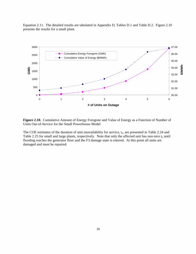
39

Equation 2.11. The detailed results are tabulated in Appendix D, Tables D.1 and Table D.2. Figure 2.10 presents the results for a small plant.

0

500

1000

1500

2000

2500

3000

0 1 2 3 4 5 6

# of Units on Outage

GW

h

30.00

31.00

32.00

33.00

34.00

35.00

36.00

37.00

$/M

Wh

Cumulative Energy Foregone (GWh) Cumulative Value of Energy ($/MWh)

Figure 2.10. Cumulative Amount of Energy Foregone and Value of Energy as a Function of Number of Units Out-of-Service for the Small Powerhouse Model The COE estimates of the duration of unit unavailability for service, tu, are presented in Table 2.24 and Table 2.25 for small and large plants, respectively. Note that only the affected unit has non-zero tu until flooding reaches the generator floor and the F3 damage state is entered. At this point all units are damaged and must be repaired.

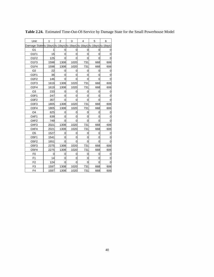
40

Table 2.24. Estimated Time-Out-Of-Service by Damage State for the Small Powerhouse Model

Unit 1 2 3 4 5 6

Damage State tu (days) tu (days) tu (days) tu (days) tu (days) tu (days)

O1 1 0 0 0 0 0

O1F1 15 0 0 0 0 0

O1F2 125 0 0 0 0 0

O1F3 1598 1308 1020 731 668 606

O1F4 1598 1308 1020 731 668 606

O2 22 0 0 0 0 0

O2F1 36 0 0 0 0 0

O2F2 146 0 0 0 0 0

O2F3 1619 1308 1020 731 668 606

O2F4 1619 1308 1020 731 668 606

O3 233 0 0 0 0 0

O3F1 247 0 0 0 0 0

O3F2 357 0 0 0 0 0

O3F3 1805 1308 1020 731 668 606

O3F4 1805 1308 1020 731 668 606

O4 625 0 0 0 0 0

O4F1 639 0 0 0 0 0

O4F2 749 0 0 0 0 0

O4F3 2021 1308 1020 731 668 606

O4F4 2021 1308 1020 731 668 606

O5 1527 0 0 0 0 0

O5F1 1541 0 0 0 0 0

O5F2 1651 0 0 0 0 0

O5F3 2275 1308 1020 731 668 606

O5F4 2275 1308 1020 731 668 606

F0 0 0 0 0 0 0

F1 14 0 0 0 0 0

F2 124 0 0 0 0 0

F3 1597 1308 1020 731 668 606

F4 1597 1308 1020 731 668 606

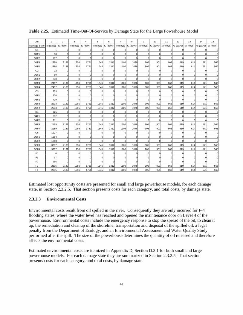
41

Table 2.25. Estimated Time-Out-Of-Service by Damage State for the Large Powerhouse Model

Unit 1 2 3 4 5 6 7 8 9 10 11 12 13 14 15

Damage State tu (days) tu (days) tu (days) tu (days) tu (days) tu (days) tu (days) tu (days) tu (days) tu (days) tu (days) tu (days) tu (days) tu (days) tu (days)

O1 1 0 0 0 0 0 0 0 0 0 0 0 0 0 0

O1F1 38 0 0 0 0 0 0 0 0 0 0 0 0 0 0

O1F2 187 0 0 0 0 0 0 0 0 0 0 0 0 0 0

O1F3 2396 2189 1956 1751 1545 1312 1106 1078 905 901 663 619 614 571 565

O1F4 2396 2189 1956 1751 1545 1312 1106 1078 905 901 663 619 614 571 565

O2 22 0 0 0 0 0 0 0 0 0 0 0 0 0 0

O2F1 59 0 0 0 0 0 0 0 0 0 0 0 0 0 0

O2F2 208 0 0 0 0 0 0 0 0 0 0 0 0 0 0

O2F3 2417 2189 1956 1751 1545 1312 1106 1078 905 901 663 619 614 571 565

O2F4 2417 2189 1956 1751 1545 1312 1106 1078 905 901 663 619 614 571 565

O3 233 0 0 0 0 0 0 0 0 0 0 0 0 0 0

O3F1 270 0 0 0 0 0 0 0 0 0 0 0 0 0 0

O3F2 419 0 0 0 0 0 0 0 0 0 0 0 0 0 0

O3F3 2603 2189 1956 1751 1545 1312 1106 1078 905 901 663 619 614 571 565

O3F4 2603 2189 1956 1751 1545 1312 1106 1078 905 901 663 619 614 571 565

O4 625 0 0 0 0 0 0 0 0 0 0 0 0 0 0

O4F1 662 0 0 0 0 0 0 0 0 0 0 0 0 0 0

O4F2 811 0 0 0 0 0 0 0 0 0 0 0 0 0 0

O4F3 2189 2189 1956 1751 1545 1312 1106 1078 905 901 663 619 614 571 565

O4F4 2189 2189 1956 1751 1545 1312 1106 1078 905 901 663 619 614 571 565

O5 1527 0 0 0 0 0 0 0 0 0 0 0 0 0 0

O5F1 1564 0 0 0 0 0 0 0 0 0 0 0 0 0 0

O5F2 1713 0 0 0 0 0 0 0 0 0 0 0 0 0 0

O5F3 3207 2189 1956 1751 1545 1312 1106 1078 905 901 663 619 614 571 565

O5F4 3207 2189 1956 1751 1545 1312 1106 1078 905 901 663 619 614 571 565

F0 0 0 0 0 0 0 0 0 0 0 0 0 0 0 0

F1 37 0 0 0 0 0 0 0 0 0 0 0 0 0 0

F2 186 0 0 0 0 0 0 0 0 0 0 0 0 0 0

F3 2395 2189 1956 1751 1545 1312 1106 1078 905 901 663 619 614 571 565

F4 2395 2189 1956 1751 1545 1312 1106 1078 905 901 663 619 614 571 565

Estimated lost opportunity costs are presented for small and large powerhouse models, for each damage state, in Section 2.3.2.5. That section presents costs for each category, and total costs, by damage state.

2.3.2.3 Environmental Costs Environmental costs result from oil spilled in the river. Consequently they are only incurred for F-4 flooding states, where the water level has reached and opened the maintenance door on Level 4 of the powerhouse. Environmental costs include the emergency response to stop the spread of the oil, to clean it up, the remediation and cleanup of the shoreline, transportation and disposal of the spilled oil, a legal penalty from the Department of Ecology, and an Environmental Assessment and Water Quality Study performed after the spill. The size of the powerhouse determines the quantity of oil released and therefore affects the environmental costs. Estimated environmental costs are itemized in Appendix D, Section D.3.1 for both small and large powerhouse models. For each damage state they are summarized in Section 2.3.2.5. That section presents costs for each category, and total costs, by damage state.

42

2.3.2.4 Interest Costs The COE calculates the costs due to interest based on single payment compound amount factor (SPCAF):

pnpiSPCAF )1( += (2.12)

where np is the number of periods and ip is the interest rate for the period. The SPCAF is used to calculate interest costs (CI) using the following relationship:

Costi

P

CostC

P

k

k

aI −

+= ∑

=

−

1

)5.(

121 (2.13)

where Cost is the cost of the work (i.e., Cc + Ce) and ia is the annual interest rate (the FY-2000 COE-established interest rate is 6.625 percent). P is the number of months the work is anticipated to take and is based on the time-to-repair (i.e., tr and te) and each month is represented by k. Estimated interest costs are presented for small and large powerhouse models, for each damage state, in the following section. That section presents costs for each category, and total costs, by damage state.

2.3.2.5 Damage State Costs The total cost for each damage state is the sum of construction costs, environmental costs, interest costs, and lost opportunity costs. Table 2.26 and Table 2.27 present the values for each of these components and the total cost for each of the 30 damage states for small and large powerhouses, respectively.

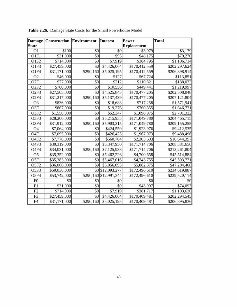
43

Table 2.26. Damage State Costs for the Small Powerhouse Model Damage State

Construction Environment Interest Power Replacement

Total

O1 $100 $0 $0 $3,079 $3,179 O1F1 $31,000 $0 $95 $48,175 $79,270 O1F2 $714,000 $0 $7,919 $384,795 $1,106,714 O1F3 $27,459,000 $0 $4,426,064 $170,412,559 $202,297,624 O1F4 $31,171,000 $290,160 $5,025,195 $170,412,559 $206,898,914

O2 $46,000 $0 $127 $67,724 $113,851 O2F1 $77,000 $0 $212 $110,821 $188,033 O2F2 $760,000 $0 $10,556 $449,441 $1,219,997 O2F3 $27,505,000 $0 $4,525,843 $170,477,205 $202,508,048 O2F4 $31,217,000 $290,160 $5,137,439 $170,477,205 $207,121,804

O3 $836,000 $0 $18,683 $717,258 $1,571,941 O3F1 $867,000 $0 $19,376 $760,355 $1,646,731 O3F2 $1,550,000 $0 $52,347 $1,098,975 $2,701,322 O3F3 $28,200,000 $0 $5,215,935 $171,049,780 $204,465,715 O3F4 $31,912,000 $290,160 $5,903,315 $171,049,780 $209,155,255

O4 $7,064,000 $0 $424,559 $1,923,976 $9,412,535 O4F1 $7,095,000 $0 $426,423 $1,967,073 $9,488,496 O4F2 $7,778,000 $0 $560,704 $2,305,693 $10,644,397 O4F3 $30,319,000 $0 $6,347,950 $171,714,706 $208,381,656 O4F4 $34,031,000 $290,160 $7,125,938 $171,714,706 $213,261,804

O5 $35,352,000 $0 $5,462,226 $4,700,658 $45,514,884 O5F1 $35,383,000 $0 $5,467,016 $4,743,755 $45,593,771 O5F2 $36,066,000 $0 $6,056,093 $5,082,375 $47,204,468 O5F3 $50,030,000 $0 $12,093,277 $172,496,610 $234,619,887 O5F4 $53,742,000 $290,160 $12,991,344 $172,496,610 $239,520,114

F0 $0 $0 $0 $0 $0 F1 $31,000 $0 $0 $43,097 $74,097 F2 $714,000 $0 $7,919 $381,717 $1,103,636 F3 $27,459,000 $0 $4,426,064 $170,409,481 $202,294,545 F4 $31,171,000 $290,160 $5,025,195 $170,409,481 $206,895,836

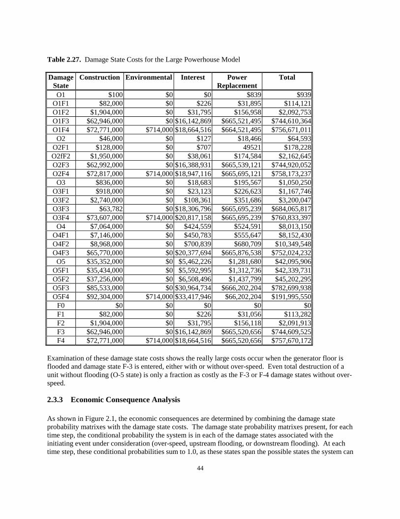
44

Table 2.27. Damage State Costs for the Large Powerhouse Model Damage

State Construction Environmental Interest Power

Replacement Total

O1 $100 $0 $0 $839 $939 O1F1 $82,000 $0 $226 $31,895 $114,121 O1F2 $1,904,000 $0 $31,795 $156,958 $2,092,753 O1F3 $62,946,000 $0 $16,142,869 $665,521,495 $744,610,364 O1F4 $72,771,000 $714,000 $18,664,516 $664,521,495 $756,671,011

O2 $46,000 $0 $127 $18,466 $64,593 O2F1 $128,000 $0 $707 49521 $178,228 O2fF2 $1,950,000 $0 $38,061 $174,584 $2,162,645 O2F3 $62,992,000 $0 $16,388,931 $665,539,121 $744,920,052 O2F4 $72,817,000 $714,000 $18,947,116 $665,695,121 $758,173,237

O3 $836,000 $0 $18,683 $195,567 $1,050,250 O3F1 $918,000 $0 $23,123 $226,623 $1,167,746 O3F2 $2,740,000 $0 $108,361 $351,686 $3,200,047 O3F3 $63,782 $0 $18,306,796 $665,695,239 $684,065,817 O3F4 $73,607,000 $714,000 $20,817,158 $665,695,239 $760,833,397

O4 $7,064,000 $0 $424,559 $524,591 $8,013,150 O4F1 $7,146,000 $0 $450,783 $555,647 $8,152,430 O4F2 $8,968,000 $0 $700,839 $680,709 $10,349,548 O4F3 $65,770,000 $0 $20,377,694 $665,876,538 $752,024,232

O5 $35,352,000 $0 $5,462,226 $1,281,680 $42,095,906 O5F1 $35,434,000 $0 $5,592,995 $1,312,736 $42,339,731 O5F2 $37,256,000 $0 $6,508,496 $1,437,799 $45,202,295 O5F3 $85,533,000 $0 $30,964,734 $666,202,204 $782,699,938 O5F4 $92,304,000 $714,000 $33,417,946 $66,202,204 $191,995,550

F0 $0 $0 $0 $0 $0 F1 $82,000 $0 $226 $31,056 $113,282 F2 $1,904,000 $0 $31,795 $156,118 $2,091,913 F3 $62,946,000 $0 $16,142,869 $665,520,656 $744,609,525 F4 $72,771,000 $714,000 $18,664,516 $665,520,656 $757,670,172

Examination of these damage state costs shows the really large costs occur when the generator floor is flooded and damage state F-3 is entered, either with or without over-speed. Even total destruction of a unit without flooding (O-5 state) is only a fraction as costly as the F-3 or F-4 damage states without over-speed.

2.3.3 Economic Consequence Analysis As shown in Figure 2.1, the economic consequences are determined by combining the damage state probability matrixes with the damage state costs. The damage state probability matrixes present, for each time step, the conditional probability the system is in each of the damage states associated with the initiating event under consideration (over-speed, upstream flooding, or downstream flooding). At each time step, these conditional probabilities sum to 1.0, as these states span the possible states the system can

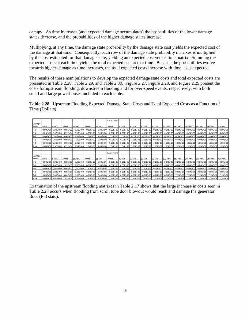
45

occupy. As time increases (and expected damage accumulates) the probabilities of the lower damage states decrease, and the probabilities of the higher damage states increase. Multiplying, at any time, the damage state probability by the damage state cost yields the expected cost of the damage at that time. Consequently, each row of the damage state probability matrixes is multiplied by the cost estimated for that damage state, yielding an expected cost versus time matrix. Summing the expected costs at each time yields the total expected cost at that time. Because the probabilities evolve towards higher damage as time increases, the total expected costs increase with time, as is expected. The results of these manipulations to develop the expected damage state costs and total expected costs are presented in Table 2.28, Table 2.29, and Table 2.30. Figure 2.27, Figure 2.28, and Figure 2.29 present the costs for upstream flooding, downstream flooding and for over-speed events, respectively, with both small and large powerhouses included in each table. Table 2.28. Upstream Flooding Expected Damage State Costs and Total Expected Costs as a Function of Time (Dollars) Examination of the upstream flooding matrixes in Table 2.17 shows that the large increase in costs seen in Table 2.28 occurs when flooding from scroll tube door blowout would reach and damage the generator floor (F-3 state).

Small Plant

Damage State 0 Min. 5 Min. 10 Min. 15 Min. 20 Min. 25 Min. 30 Min. 40 Min. 50 Min. 60 Min. 90 Min. 120 Min. 180 Min. 240 Min. 300 Min. 360 Min. 420 Min.

F-0 0.00E+00 0.00E+00 0.00E+00 0.00E+00 0.00E+00 0.00E+00 0.00E+00 0.00E+00 0.00E+00 0.00E+00 0.00E+00 0.00E+00 0.00E+00 0.00E+00 0.00E+00 0.00E+00 0.00E+00

F-1 0.00E+00 6.97E+04 6.97E+04 0.00E+00 0.00E+00 0.00E+00 0.00E+00 0.00E+00 4.45E+03 4.45E+03 4.45E+03 4.45E+03 4.45E+03 4.45E+03 4.45E+03 4.45E+03 4.45E+03

F-2 0.00E+00 0.00E+00 0.00E+00 1.04E+06 1.04E+06 1.04E+06 1.04E+06 1.04E+06 0.00E+00 0.00E+00 0.00E+00 0.00E+00 0.00E+00 0.00E+00 0.00E+00 0.00E+00 0.00E+00

F-3 0.00E+00 0.00E+00 0.00E+00 0.00E+00 0.00E+00 0.00E+00 0.00E+00 0.00E+00 1.91E+08 1.91E+08 0.00E+00 0.00E+00 0.00E+00 0.00E+00 0.00E+00 0.00E+00 0.00E+00

F-4 0.00E+00 0.00E+00 0.00E+00 0.00E+00 0.00E+00 0.00E+00 0.00E+00 0.00E+00 0.00E+00 0.00E+00 1.95E+08 1.95E+08 1.95E+08 1.95E+08 1.95E+08 1.95E+08 1.95E+08

Total 0.00E+00 6.97E+04 6.97E+04 1.04E+06 1.04E+06 1.04E+06 1.04E+06 1.04E+06 1.91E+08 1.91E+08 1.95E+08 1.95E+08 1.95E+08 1.95E+08 1.95E+08 1.95E+08 1.95E+08

Large Plant

Damage State 0 Min. 5 Min. 10 Min. 15 Min. 20 Min. 25 Min. 30 Min. 40 Min. 50 Min. 60 Min. 90 Min. 120 Min. 180 Min. 240 Min. 300 Min. 360 Min. 420 Min.

F-0 0.00E+00 0.00E+00 0.00E+00 0.00E+00 0.00E+00 0.00E+00 0.00E+00 0.00E+00 0.00E+00 0.00E+00 0.00E+00 0.00E+00 0.00E+00 0.00E+00 0.00E+00 0.00E+00 0.00E+00

F-1 0.00E+00 1.07E+05 1.07E+05 1.07E+05 0.00E+00 0.00E+00 0.00E+00 0.00E+00 0.00E+00 0.00E+00 6.80E+03 6.80E+03 6.80E+03 6.80E+03 6.80E+03 6.80E+03 6.80E+03

F-2 0.00E+00 0.00E+00 0.00E+00 0.00E+00 1.97E+06 1.97E+06 1.97E+06 1.97E+06 1.97E+06 1.97E+06 0.00E+00 0.00E+00 0.00E+00 0.00E+00 0.00E+00 0.00E+00 0.00E+00

F-3 0.00E+00 0.00E+00 0.00E+00 0.00E+00 0.00E+00 0.00E+00 0.00E+00 0.00E+00 0.00E+00 0.00E+00 7.03E+08 7.03E+08 0.00E+00 0.00E+00 0.00E+00 0.00E+00 0.00E+00

F-4 0.00E+00 0.00E+00 0.00E+00 0.00E+00 0.00E+00 0.00E+00 0.00E+00 0.00E+00 0.00E+00 0.00E+00 0.00E+00 0.00E+00 7.15E+08 7.15E+08 7.15E+08 7.15E+08 7.15E+08

Total 0.00E+00 1.07E+05 1.07E+05 1.07E+05 1.97E+06 1.97E+06 1.97E+06 1.97E+06 1.97E+06 1.97E+06 7.03E+08 7.03E+08 7.15E+08 7.15E+08 7.15E+08 7.15E+08 7.15E+08

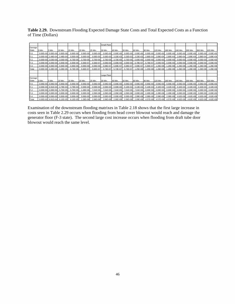
46

Table 2.29. Downstream Flooding Expected Damage State Costs and Total Expected Costs as a Function of Time (Dollars) Examination of the downstream flooding matrixes in Table 2.18 shows that the first large increase in costs seen in Table 2.29 occurs when flooding from head cover blowout would reach and damage the generator floor (F-3 state). The second large cost increase occurs when flooding from draft tube door blowout would reach the same level.

Small Plant

Damage State 0 Min. 5 Min. 10 Min. 15 Min. 20 Min. 25 Min. 30 Min. 40 Min. 50 Min. 60 Min. 90 Min. 120 Min. 180 Min. 240 Min. 300 Min. 360 Min. 420 Min.

F-0 0.00E+00 0.00E+00 0.00E+00 0.00E+00 0.00E+00 0.00E+00 0.00E+00 0.00E+00 0.00E+00 0.00E+00 0.00E+00 0.00E+00 0.00E+00 0.00E+00 0.00E+00 0.00E+00 0.00E+00

F-1 0.00E+00 2.48E+04 2.48E+04 0.00E+00 0.00E+00 0.00E+00 0.00E+00 3.33E+03 3.33E+03 3.33E+03 2.89E+04 2.89E+04 2.89E+04 2.89E+04 2.89E+04 2.89E+04 2.89E+04

F-2 0.00E+00 3.03E+05 3.03E+05 6.73E+05 3.70E+05 3.70E+05 3.70E+05 3.70E+05 3.70E+05 0.00E+00 0.00E+00 0.00E+00 0.00E+00 0.00E+00 0.00E+00 0.00E+00 0.00E+00

F-3 0.00E+00 0.00E+00 0.00E+00 0.00E+00 5.56E+07 5.56E+07 0.00E+00 0.00E+00 0.00E+00 6.78E+07 6.78E+07 0.00E+00 0.00E+00 0.00E+00 0.00E+00 0.00E+00 0.00E+00

F-4 0.00E+00 0.00E+00 0.00E+00 0.00E+00 0.00E+00 0.00E+00 5.69E+07 5.69E+07 5.69E+07 5.69E+07 5.69E+07 1.26E+08 1.26E+08 1.26E+08 1.26E+08 1.26E+08 1.26E+08

Total 0.00E+00 3.28E+05 3.28E+05 6.73E+05 5.60E+07 5.60E+07 5.73E+07 5.73E+07 5.73E+07 1.25E+08 1.25E+08 1.26E+08 1.26E+08 1.26E+08 1.26E+08 1.26E+08 1.26E+08

Large Plant

Damage State 0 Min. 5 Min. 10 Min. 15 Min. 20 Min. 25 Min. 30 Min. 40 Min. 50 Min. 60 Min. 90 Min. 120 Min. 180 Min. 240 Min. 300 Min. 360 Min. 420 Min.

F-0 0.00E+00 0.00E+00 0.00E+00 0.00E+00 0.00E+00 0.00E+00 0.00E+00 0.00E+00 0.00E+00 0.00E+00 0.00E+00 0.00E+00 0.00E+00 0.00E+00 0.00E+00 0.00E+00 0.00E+00

F-1 0.00E+00 6.91E+04 3.79E+04 3.79E+04 0.00E+00 0.00E+00 0.00E+00 0.00E+00 5.10E+03 5.10E+03 5.10E+03 4.42E+04 4.42E+04 4.42E+04 4.42E+04 4.42E+04 4.42E+04

F-2 0.00E+00 0.00E+00 5.75E+05 5.75E+05 1.28E+06 7.01E+05 7.01E+05 7.01E+05 7.01E+05 7.01E+05 0.00E+00 0.00E+00 0.00E+00 0.00E+00 0.00E+00 0.00E+00 0.00E+00

F-3 0.00E+00 0.00E+00 0.00E+00 0.00E+00 0.00E+00 2.05E+08 2.05E+08 2.05E+08 2.05E+08 0.00E+00 2.49E+08 2.49E+08 2.49E+08 0.00E+00 0.00E+00 0.00E+00 0.00E+00

F-4 0.00E+00 0.00E+00 0.00E+00 0.00E+00 0.00E+00 0.00E+00 0.00E+00 0.00E+00 0.00E+00 2.08E+08 2.08E+08 2.08E+08 2.08E+08 4.62E+08 4.62E+08 4.62E+08 4.62E+08

Total 0.00E+00 6.91E+04 6.13E+05 6.13E+05 1.28E+06 2.06E+08 2.06E+08 2.06E+08 2.06E+08 2.09E+08 4.57E+08 4.57E+08 4.57E+08 4.62E+08 4.62E+08 4.62E+08 4.62E+08

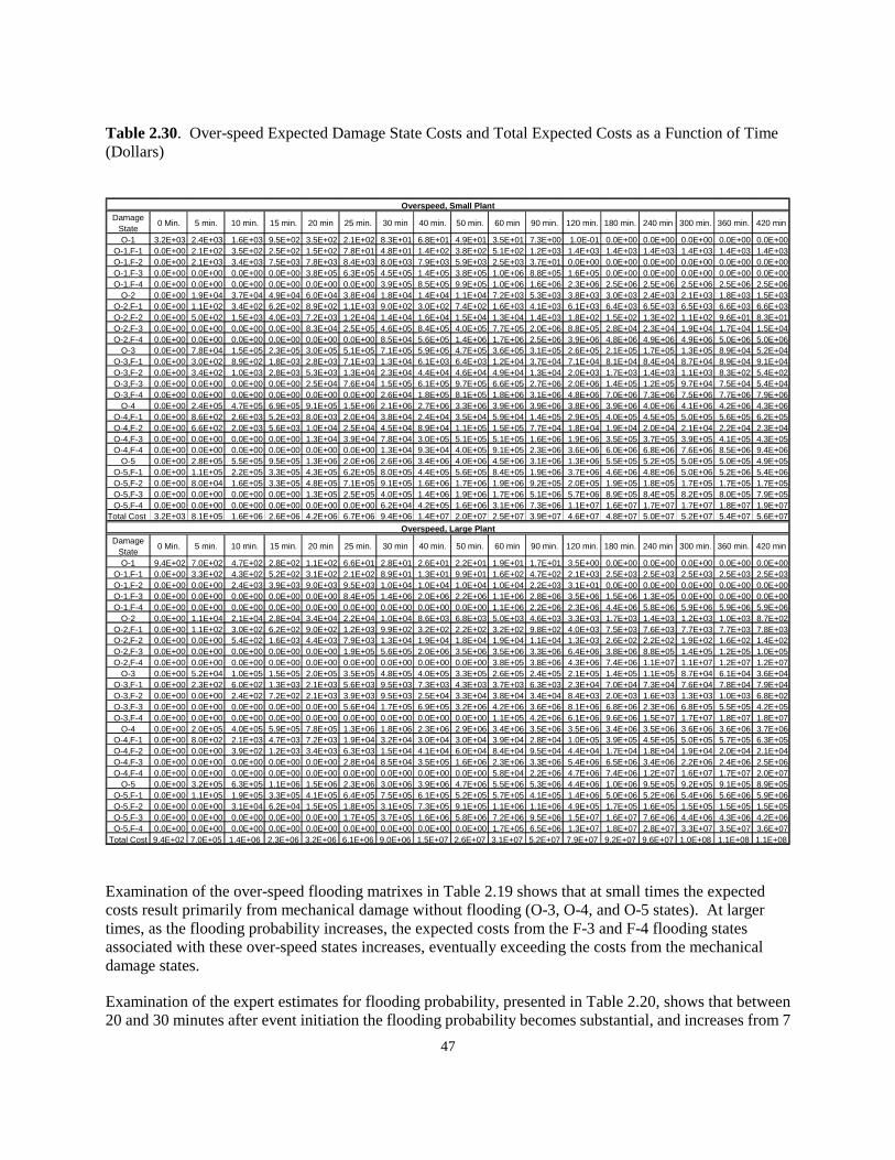
47

Table 2.30. Over-speed Expected Damage State Costs and Total Expected Costs as a Function of Time (Dollars)

Overspeed, Small PlantDamage

State0 Min. 5 min. 10 min. 15 min. 20 min 25 min. 30 min 40 min. 50 min. 60 min 90 min. 120 min. 180 min. 240 min 300 min. 360 min. 420 min

O-1 3.2E+03 2.4E+03 1.6E+03 9.5E+02 3.5E+02 2.1E+02 8.3E+01 6.8E+01 4.9E+01 3.5E+01 7.3E+00 1.0E-01 0.0E+00 0.0E+00 0.0E+00 0.0E+00 0.0E+00O-1,F-1 0.0E+00 2.1E+02 3.5E+02 2.5E+02 1.5E+02 7.8E+01 4.8E+01 1.4E+02 3.8E+02 5.1E+02 1.2E+03 1.4E+03 1.4E+03 1.4E+03 1.4E+03 1.4E+03 1.4E+03O-1,F-2 0.0E+00 2.1E+03 3.4E+03 7.5E+03 7.8E+03 8.4E+03 8.0E+03 7.9E+03 5.9E+03 2.5E+03 3.7E+01 0.0E+00 0.0E+00 0.0E+00 0.0E+00 0.0E+00 0.0E+00O-1,F-3 0.0E+00 0.0E+00 0.0E+00 0.0E+00 3.8E+05 6.3E+05 4.5E+05 1.4E+05 3.8E+05 1.0E+06 8.8E+05 1.6E+05 0.0E+00 0.0E+00 0.0E+00 0.0E+00 0.0E+00O-1,F-4 0.0E+00 0.0E+00 0.0E+00 0.0E+00 0.0E+00 0.0E+00 3.9E+05 8.5E+05 9.9E+05 1.0E+06 1.6E+06 2.3E+06 2.5E+06 2.5E+06 2.5E+06 2.5E+06 2.5E+06

O-2 0.0E+00 1.9E+04 3.7E+04 4.9E+04 6.0E+04 3.8E+04 1.8E+04 1.4E+04 1.1E+04 7.2E+03 5.3E+03 3.8E+03 3.0E+03 2.4E+03 2.1E+03 1.8E+03 1.5E+03O-2,F-1 0.0E+00 1.1E+02 3.4E+02 6.2E+02 8.9E+02 1.1E+03 9.0E+02 3.0E+02 7.4E+02 1.6E+03 4.1E+03 6.1E+03 6.4E+03 6.5E+03 6.5E+03 6.6E+03 6.6E+03O-2,F-2 0.0E+00 5.0E+02 1.5E+03 4.0E+03 7.2E+03 1.2E+04 1.4E+04 1.6E+04 1.5E+04 1.3E+04 1.4E+03 1.8E+02 1.5E+02 1.3E+02 1.1E+02 9.6E+01 8.3E+01O-2,F-3 0.0E+00 0.0E+00 0.0E+00 0.0E+00 8.3E+04 2.5E+05 4.6E+05 8.4E+05 4.0E+05 7.7E+05 2.0E+06 8.8E+05 2.8E+04 2.3E+04 1.9E+04 1.7E+04 1.5E+04O-2,F-4 0.0E+00 0.0E+00 0.0E+00 0.0E+00 0.0E+00 0.0E+00 8.5E+04 5.6E+05 1.4E+06 1.7E+06 2.5E+06 3.9E+06 4.8E+06 4.9E+06 4.9E+06 5.0E+06 5.0E+06

O-3 0.0E+00 7.8E+04 1.5E+05 2.3E+05 3.0E+05 5.1E+05 7.1E+05 5.9E+05 4.7E+05 3.6E+05 3.1E+05 2.6E+05 2.1E+05 1.7E+05 1.3E+05 8.9E+04 5.2E+04O-3,F-1 0.0E+00 3.0E+02 8.9E+02 1.8E+03 2.8E+03 7.1E+03 1.3E+04 6.1E+03 6.4E+03 1.2E+04 3.7E+04 7.1E+04 8.1E+04 8.4E+04 8.7E+04 8.9E+04 9.1E+04O-3,F-2 0.0E+00 3.4E+02 1.0E+03 2.8E+03 5.3E+03 1.3E+04 2.3E+04 4.4E+04 4.6E+04 4.9E+04 1.3E+04 2.0E+03 1.7E+03 1.4E+03 1.1E+03 8.3E+02 5.4E+02O-3,F-3 0.0E+00 0.0E+00 0.0E+00 0.0E+00 2.5E+04 7.6E+04 1.5E+05 6.1E+05 9.7E+05 6.6E+05 2.7E+06 2.0E+06 1.4E+05 1.2E+05 9.7E+04 7.5E+04 5.4E+04O-3,F-4 0.0E+00 0.0E+00 0.0E+00 0.0E+00 0.0E+00 0.0E+00 2.6E+04 1.8E+05 8.1E+05 1.8E+06 3.1E+06 4.8E+06 7.0E+06 7.3E+06 7.5E+06 7.7E+06 7.9E+06

O-4 0.0E+00 2.4E+05 4.7E+05 6.9E+05 9.1E+05 1.5E+06 2.1E+06 2.7E+06 3.3E+06 3.9E+06 3.9E+06 3.8E+06 3.9E+06 4.0E+06 4.1E+06 4.2E+06 4.3E+06O-4,F-1 0.0E+00 8.6E+02 2.6E+03 5.2E+03 8.0E+03 2.0E+04 3.8E+04 2.4E+04 3.5E+04 5.9E+04 1.4E+05 2.9E+05 4.0E+05 4.5E+05 5.0E+05 5.6E+05 6.2E+05O-4,F-2 0.0E+00 6.6E+02 2.0E+03 5.6E+03 1.0E+04 2.5E+04 4.5E+04 8.9E+04 1.1E+05 1.5E+05 7.7E+04 1.8E+04 1.9E+04 2.0E+04 2.1E+04 2.2E+04 2.3E+04O-4,F-3 0.0E+00 0.0E+00 0.0E+00 0.0E+00 1.3E+04 3.9E+04 7.8E+04 3.0E+05 5.1E+05 5.1E+05 1.6E+06 1.9E+06 3.5E+05 3.7E+05 3.9E+05 4.1E+05 4.3E+05O-4,F-4 0.0E+00 0.0E+00 0.0E+00 0.0E+00 0.0E+00 0.0E+00 1.3E+04 9.3E+04 4.0E+05 9.1E+05 2.3E+06 3.6E+06 6.0E+06 6.8E+06 7.6E+06 8.5E+06 9.4E+06

O-5 0.0E+00 2.8E+05 5.5E+05 9.5E+05 1.3E+06 2.0E+06 2.6E+06 3.4E+06 4.0E+06 4.5E+06 3.1E+06 1.3E+06 5.5E+05 5.2E+05 5.0E+05 5.0E+05 4.9E+05O-5,F-1 0.0E+00 1.1E+05 2.2E+05 3.3E+05 4.3E+05 6.2E+05 8.0E+05 4.4E+05 5.6E+05 8.4E+05 1.9E+06 3.7E+06 4.6E+06 4.8E+06 5.0E+06 5.2E+06 5.4E+06O-5,F-2 0.0E+00 8.0E+04 1.6E+05 3.3E+05 4.8E+05 7.1E+05 9.1E+05 1.6E+06 1.7E+06 1.9E+06 9.2E+05 2.0E+05 1.9E+05 1.8E+05 1.7E+05 1.7E+05 1.7E+05O-5,F-3 0.0E+00 0.0E+00 0.0E+00 0.0E+00 1.3E+05 2.5E+05 4.0E+05 1.4E+06 1.9E+06 1.7E+06 5.1E+06 5.7E+06 8.9E+05 8.4E+05 8.2E+05 8.0E+05 7.9E+05O-5,F-4 0.0E+00 0.0E+00 0.0E+00 0.0E+00 0.0E+00 0.0E+00 6.2E+04 4.2E+05 1.6E+06 3.1E+06 7.3E+06 1.1E+07 1.6E+07 1.7E+07 1.7E+07 1.8E+07 1.9E+07

Total Cost 3.2E+03 8.1E+05 1.6E+06 2.6E+06 4.2E+06 6.7E+06 9.4E+06 1.4E+07 2.0E+07 2.5E+07 3.9E+07 4.6E+07 4.8E+07 5.0E+07 5.2E+07 5.4E+07 5.6E+07

Overspeed, Large PlantDamage

State0 Min. 5 min. 10 min. 15 min. 20 min 25 min. 30 min 40 min. 50 min. 60 min 90 min. 120 min. 180 min. 240 min 300 min. 360 min. 420 min

O-1 9.4E+02 7.0E+02 4.7E+02 2.8E+02 1.1E+02 6.6E+01 2.8E+01 2.6E+01 2.2E+01 1.9E+01 1.7E+01 3.5E+00 0.0E+00 0.0E+00 0.0E+00 0.0E+00 0.0E+00O-1,F-1 0.0E+00 3.3E+02 4.3E+02 5.2E+02 3.1E+02 2.1E+02 8.9E+01 1.3E+01 9.9E+01 1.6E+02 4.7E+02 2.1E+03 2.5E+03 2.5E+03 2.5E+03 2.5E+03 2.5E+03O-1,F-2 0.0E+00 0.0E+00 2.4E+03 3.9E+03 9.0E+03 9.5E+03 1.0E+04 1.0E+04 1.0E+04 1.0E+04 2.2E+03 3.1E+01 0.0E+00 0.0E+00 0.0E+00 0.0E+00 0.0E+00O-1,F-3 0.0E+00 0.0E+00 0.0E+00 0.0E+00 0.0E+00 8.4E+05 1.4E+06 2.0E+06 2.2E+06 1.1E+06 2.8E+06 3.5E+06 1.5E+06 1.3E+05 0.0E+00 0.0E+00 0.0E+00O-1,F-4 0.0E+00 0.0E+00 0.0E+00 0.0E+00 0.0E+00 0.0E+00 0.0E+00 0.0E+00 0.0E+00 1.1E+06 2.2E+06 2.3E+06 4.4E+06 5.8E+06 5.9E+06 5.9E+06 5.9E+06

O-2 0.0E+00 1.1E+04 2.1E+04 2.8E+04 3.4E+04 2.2E+04 1.0E+04 8.6E+03 6.8E+03 5.0E+03 4.6E+03 3.3E+03 1.7E+03 1.4E+03 1.2E+03 1.0E+03 8.7E+02O-2,F-1 0.0E+00 1.1E+02 3.0E+02 6.2E+02 9.0E+02 1.2E+03 9.9E+02 3.2E+02 2.2E+02 3.2E+02 9.8E+02 4.0E+03 7.5E+03 7.6E+03 7.7E+03 7.7E+03 7.8E+03O-2,F-2 0.0E+00 0.0E+00 5.4E+02 1.6E+03 4.4E+03 7.9E+03 1.3E+04 1.9E+04 1.8E+04 1.9E+04 1.1E+04 1.3E+03 2.6E+02 2.2E+02 1.9E+02 1.6E+02 1.4E+02O-2,F-3 0.0E+00 0.0E+00 0.0E+00 0.0E+00 0.0E+00 1.9E+05 5.6E+05 2.0E+06 3.5E+06 3.5E+06 3.3E+06 6.4E+06 3.8E+06 8.8E+05 1.4E+05 1.2E+05 1.0E+05O-2,F-4 0.0E+00 0.0E+00 0.0E+00 0.0E+00 0.0E+00 0.0E+00 0.0E+00 0.0E+00 0.0E+00 3.8E+05 3.8E+06 4.3E+06 7.4E+06 1.1E+07 1.1E+07 1.2E+07 1.2E+07

O-3 0.0E+00 5.2E+04 1.0E+05 1.5E+05 2.0E+05 3.5E+05 4.8E+05 4.0E+05 3.3E+05 2.6E+05 2.4E+05 2.1E+05 1.4E+05 1.1E+05 8.7E+04 6.1E+04 3.6E+04O-3,F-1 0.0E+00 2.3E+02 6.0E+02 1.3E+03 2.1E+03 5.6E+03 9.5E+03 7.3E+03 4.3E+03 3.7E+03 6.3E+03 2.3E+04 7.0E+04 7.3E+04 7.6E+04 7.8E+04 7.9E+04O-3,F-2 0.0E+00 0.0E+00 2.4E+02 7.2E+02 2.1E+03 3.9E+03 9.5E+03 2.5E+04 3.3E+04 3.8E+04 3.4E+04 8.4E+03 2.0E+03 1.6E+03 1.3E+03 1.0E+03 6.8E+02O-3,F-3 0.0E+00 0.0E+00 0.0E+00 0.0E+00 0.0E+00 5.6E+04 1.7E+05 6.9E+05 3.2E+06 4.2E+06 3.6E+06 8.1E+06 6.8E+06 2.3E+06 6.8E+05 5.5E+05 4.2E+05O-3,F-4 0.0E+00 0.0E+00 0.0E+00 0.0E+00 0.0E+00 0.0E+00 0.0E+00 0.0E+00 0.0E+00 1.1E+05 4.2E+06 6.1E+06 9.6E+06 1.5E+07 1.7E+07 1.8E+07 1.8E+07

O-4 0.0E+00 2.0E+05 4.0E+05 5.9E+05 7.8E+05 1.3E+06 1.8E+06 2.3E+06 2.9E+06 3.4E+06 3.5E+06 3.5E+06 3.4E+06 3.5E+06 3.6E+06 3.6E+06 3.7E+06O-4,F-1 0.0E+00 8.0E+02 2.1E+03 4.7E+03 7.2E+03 1.9E+04 3.2E+04 3.0E+04 3.0E+04 3.9E+04 2.8E+04 1.0E+05 3.9E+05 4.5E+05 5.0E+05 5.7E+05 6.3E+05O-4,F-2 0.0E+00 0.0E+00 3.9E+02 1.2E+03 3.4E+03 6.3E+03 1.5E+04 4.1E+04 6.0E+04 8.4E+04 9.5E+04 4.4E+04 1.7E+04 1.8E+04 1.9E+04 2.0E+04 2.1E+04O-4,F-3 0.0E+00 0.0E+00 0.0E+00 0.0E+00 0.0E+00 2.8E+04 8.5E+04 3.5E+05 1.6E+06 2.3E+06 3.3E+06 5.4E+06 6.5E+06 3.4E+06 2.2E+06 2.4E+06 2.5E+06O-4,F-4 0.0E+00 0.0E+00 0.0E+00 0.0E+00 0.0E+00 0.0E+00 0.0E+00 0.0E+00 0.0E+00 5.8E+04 2.2E+06 4.7E+06 7.4E+06 1.2E+07 1.6E+07 1.7E+07 2.0E+07

O-5 0.0E+00 3.2E+05 6.3E+05 1.1E+06 1.5E+06 2.3E+06 3.0E+06 3.9E+06 4.7E+06 5.5E+06 5.3E+06 4.4E+06 1.0E+06 9.5E+05 9.2E+05 9.1E+05 8.9E+05O-5,F-1 0.0E+00 1.1E+05 1.9E+05 3.3E+05 4.1E+05 6.4E+05 7.5E+05 6.1E+05 5.2E+05 5.7E+05 4.1E+05 1.4E+06 5.0E+06 5.2E+06 5.4E+06 5.6E+06 5.9E+06O-5,F-2 0.0E+00 0.0E+00 3.1E+04 6.2E+04 1.5E+05 1.8E+05 3.1E+05 7.3E+05 9.1E+05 1.1E+06 1.1E+06 4.9E+05 1.7E+05 1.6E+05 1.5E+05 1.5E+05 1.5E+05O-5,F-3 0.0E+00 0.0E+00 0.0E+00 0.0E+00 0.0E+00 1.7E+05 3.7E+05 1.6E+06 5.8E+06 7.2E+06 9.5E+06 1.5E+07 1.6E+07 7.6E+06 4.4E+06 4.3E+06 4.2E+06O-5,F-4 0.0E+00 0.0E+00 0.0E+00 0.0E+00 0.0E+00 0.0E+00 0.0E+00 0.0E+00 0.0E+00 1.7E+05 6.5E+06 1.3E+07 1.8E+07 2.8E+07 3.3E+07 3.5E+07 3.6E+07

Total Cost 9.4E+02 7.0E+05 1.4E+06 2.3E+06 3.2E+06 6.1E+06 9.0E+06 1.5E+07 2.6E+07 3.1E+07 5.2E+07 7.9E+07 9.2E+07 9.6E+07 1.0E+08 1.1E+08 1.1E+08 Examination of the over-speed flooding matrixes in Table 2.19 shows that at small times the expected costs result primarily from mechanical damage without flooding (O-3, O-4, and O-5 states). At larger times, as the flooding probability increases, the expected costs from the F-3 and F-4 flooding states associated with these over-speed states increases, eventually exceeding the costs from the mechanical damage states.

Examination of the expert estimates for flooding probability, presented in Table 2.20, shows that between 20 and 30 minutes after event initiation the flooding probability becomes substantial, and increases from 7

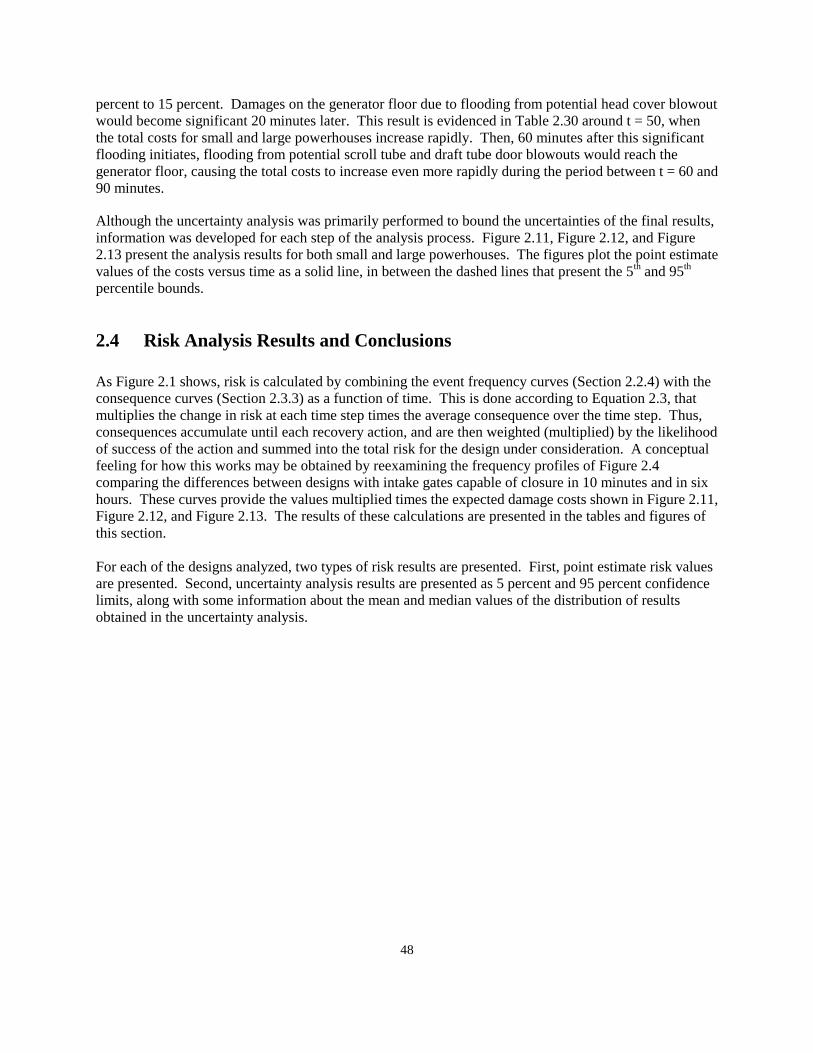
48

percent to 15 percent. Damages on the generator floor due to flooding from potential head cover blowout would become significant 20 minutes later. This result is evidenced in Table 2.30 around t = 50, when the total costs for small and large powerhouses increase rapidly. Then, 60 minutes after this significant flooding initiates, flooding from potential scroll tube and draft tube door blowouts would reach the generator floor, causing the total costs to increase even more rapidly during the period between t = 60 and 90 minutes.

Although the uncertainty analysis was primarily performed to bound the uncertainties of the final results, information was developed for each step of the analysis process. Figure 2.11, Figure 2.12, and Figure 2.13 present the analysis results for both small and large powerhouses. The figures plot the point estimate values of the costs versus time as a solid line, in between the dashed lines that present the 5th and 95th

percentile bounds.

2.4 Risk Analysis Results and Conclusions As Figure 2.1 shows, risk is calculated by combining the event frequency curves (Section 2.2.4) with the consequence curves (Section 2.3.3) as a function of time. This is done according to Equation 2.3, that multiplies the change in risk at each time step times the average consequence over the time step. Thus, consequences accumulate until each recovery action, and are then weighted (multiplied) by the likelihood of success of the action and summed into the total risk for the design under consideration. A conceptual feeling for how this works may be obtained by reexamining the frequency profiles of Figure 2.4 comparing the differences between designs with intake gates capable of closure in 10 minutes and in six hours. These curves provide the values multiplied times the expected damage costs shown in Figure 2.11, Figure 2.12, and Figure 2.13. The results of these calculations are presented in the tables and figures of this section. For each of the designs analyzed, two types of risk results are presented. First, point estimate risk values are presented. Second, uncertainty analysis results are presented as 5 percent and 95 percent confidence limits, along with some information about the mean and median values of the distribution of results obtained in the uncertainty analysis.

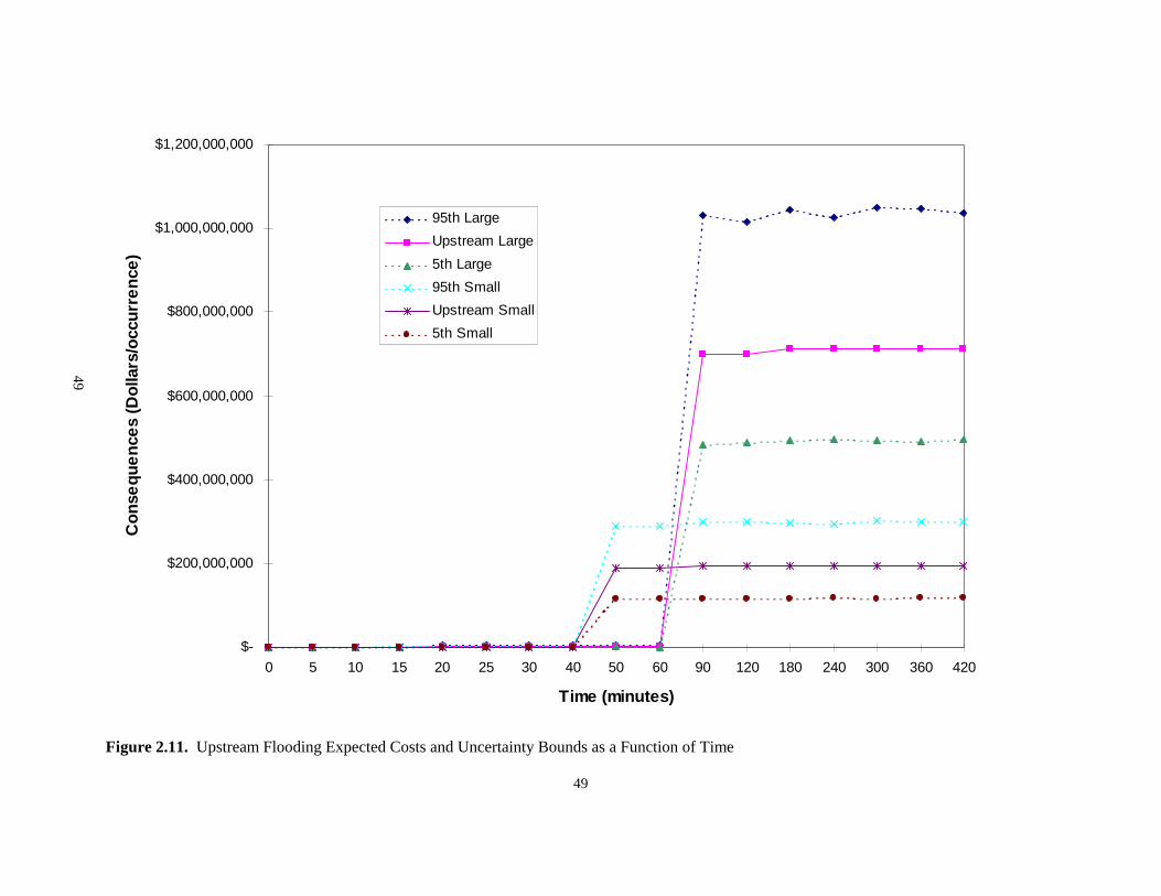
49

Figure 2.11. Upstream Flooding Expected Costs and Uncertainty Bounds as a Function of Time

$-

$200,000,000

$400,000,000

$600,000,000

$800,000,000

$1,000,000,000

$1,200,000,000

0 5 10 15 20 25 30 40 50 60 90 120 180 240 300 360 420

Time (minutes)

Co

nse

qu

en

ces

(Do

llars

/occ

urr

en

ce)

95th Large

Upstream Large

5th Large

95th Small

Upstream Small

5th Small

49

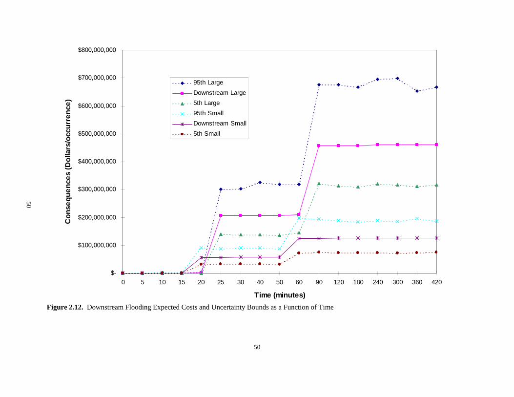
50

Figure 2.12. Downstream Flooding Expected Costs and Uncertainty Bounds as a Function of Time

$-

$100,000,000

$200,000,000

$300,000,000

$400,000,000

$500,000,000

$600,000,000

$700,000,000

$800,000,000

0 5 10 15 20 25 30 40 50 60 90 120 180 240 300 360 420

Time (minutes)

Co

nse

qu

en

ces

(Do

llars

/occ

urr

en

ce)

95th Large

Downstream Large

5th Large

95th Small

Downstream Small

5th Small

50

51

Figure 2.13. Over-speed Expected Costs and Uncertainty Bounds as a Function of Time

$-

$50,000,000

$100,000,000

$150,000,000

$200,000,000

$250,000,000

$300,000,000

0 5 10 15 20 25 30 40 50 60 90 120 180 240 300 360 420

Time (minutes)

Co

nse

qu

en

ces

(Do

llars

/occ

urr

en

ce)

95th Large

Overspeed Large

5th Large

95th Small

Overspeed Small

5th Small

51

52

2.4.1 Risk Point Estimate Results and Conclusions The point estimate total risk values obtained for small powerhouse designs are presented in Table 2.31. Table 2.32 presents the comparable values for large powerhouse designs. Table 2.31. Total Risk Point Estimates for the Small Powerhouse Model ($ M/unit-yr.)

Intake Gate Closure Time Small Powerhouse Design 10 min. 30 min. 60 min. 360 min. HY-N (Des. 11) 1.12 1.16 2.49 HY-T (Des. 3) 1.14 1.17 2.49 HY-F (Des. 7) 1.19 1.22 2.50 HY-T-E (Des. 15) 1.13 1.16 2.44 HY-F-E (Des. 19) 1.16 1.19 2.45 HO-T-E (Des. 14) 1.15 1.17 2.44 HO-F-E (Des. 18) 1.18 1.20 2.45 CR-N (Des. 12) 1.20 2.39 2.49 CR-T (Des. 4) 1.25 2.40 2.50 CR-F (Des. 8) 1.30 2.43 2.50 CR-T-E (Des. 16) 1.24 2.37 2.45 CR-F-E (Des. 20) 1.27 2.39 2.45 Table 2.32. Total Risk Point Estimates for the Large Powerhouse Model ($ M/unit-yr.)

Intake Gate Closure Time Large Powerhouse Design 10 min. 30 min. 60 min. 360 min. HY-N (Des. 11) 1.09 1.13 5.99 HY-T (Des. 3) 1.14 1.18 6.01 HY-F (Des. 7) 1.26 1.32 6.03 HY-T-E (Des. 15) 1.12 1.16 5.87 HY-F-E (Des. 19) 1.22 1.25 5.88 HO-T-E (Des. 14) 1.16 1.20 5.87 HO-F-E (Des. 18) 1.26 1.30 5.88 CR-N (Des. 12) 1.43 1.52 5.99 CR-T (Des. 4) 1.48 1.57 6.02 CR-F (Des. 8) 1.62 1.68 6.03 CR-T-E (Des. 16) 1.45 1.50 5.87 CR-F-E (Des. 20) 1.55 1.59 5.88

53

Examination of the total risk values presented in Table 2.31 and Table 2.32 leads to the following conclusions: • The primary determinant of total risk is the time required to close the intake gates after occurrence of

an initiating event. The risk is much greater for designs requiring six hours for intake gate closure than for designs requiring 10 minutes or 30 minutes for closure.

• For small powerhouses, total risk increases rapidly for designs requiring more than 30 minutes for

intake gate closure, and approaches its maximum value for designs requiring 60 minutes. For large powerhouses the major risk increase occurs for designs requiring more than 60 minutes to close the intake gates. (This difference is because flooding takes longer to fill the lower elevations of the large powerhouses before it reaches the generator floor.)

• Emergency closure systems for the wicket gates reduce the total risk from 0 to 5 percent, depending

on design details. • Fish screens increase the total risk from 0 to 6 percent for small powerhouses, and from 1 to 12

percent for large powerhouses, depending on design details. Fixed bar fish screens increase the risk more than traveling mesh fish screens.

The point estimate values of the risk contributions to total risk from over-speed, upstream flooding, and downstream flooding obtained for small powerhouse designs are presented in Table 2.33. Table 2.34 presents the comparable values for large powerhouse designs.

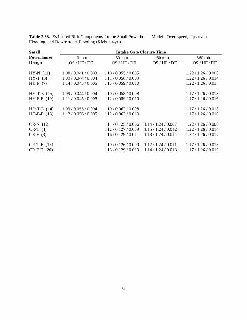
54

Table 2.33. Estimated Risk Components for the Small Powerhouse Model: Over-speed, Upstream Flooding, and Downstream Flooding ($ M/unit-yr.)

Intake Gate Closure Time 10 min 30 min 60 min 360 min

Small Powerhouse Design OS / UF / DF OS / UF / DF OS / UF / DF OS / UF / DF HY-N (11) 1.08 / 0.041 / 0.003 1.10 / 0.055 / 0.005 1.22 / 1.26 / 0.008 HY-T (3) 1.09 / 0.044 / 0.004 1.11 / 0.058 / 0.009 1.22 / 1.26 / 0.014 HY-F (7) 1.14 / 0.045 / 0.005 1.15 / 0.059 / 0.010 1.22 / 1.26 / 0.017 HY-T-E (15) 1.09 / 0.044 / 0.004 1.10 / 0.058 / 0.008 1.17 / 1.26 / 0.013 HY-F-E (19) 1.11 / 0.045 / 0.005 1.12 / 0.059 / 0.010 1.17 / 1.26 / 0.016 HO-T-E (14) 1.09 / 0.055 / 0.004 1.10 / 0.062 / 0.008 1.17 / 1.26 / 0.013 HO-F-E (18) 1.12 / 0.056 / 0.005 1.12 / 0.063 / 0.010 1.17 / 1.26 / 0.016 CR-N (12) 1.11 / 0.125 / 0.006 1.14 / 1.24 / 0.007 1.22 / 1.26 / 0.008 CR-T (4) 1.12 / 0.127 / 0.009 1.15 / 1.24 / 0.012 1.22 / 1.26 / 0.014 CR-F (8) 1.16 / 0.129 / 0.011 1.18 / 1.24 / 0.014 1.22 / 1.26 / 0.017 CR-T-E (16) 1.10 / 0.126 / 0.009 1.12 / 1.24 / 0.011 1.17 / 1.26 / 0.013 CR-F-E (20) 1.13 / 0.129 / 0.010 1.14 / 1.24 / 0.013 1.17 / 1.26 / 0.016

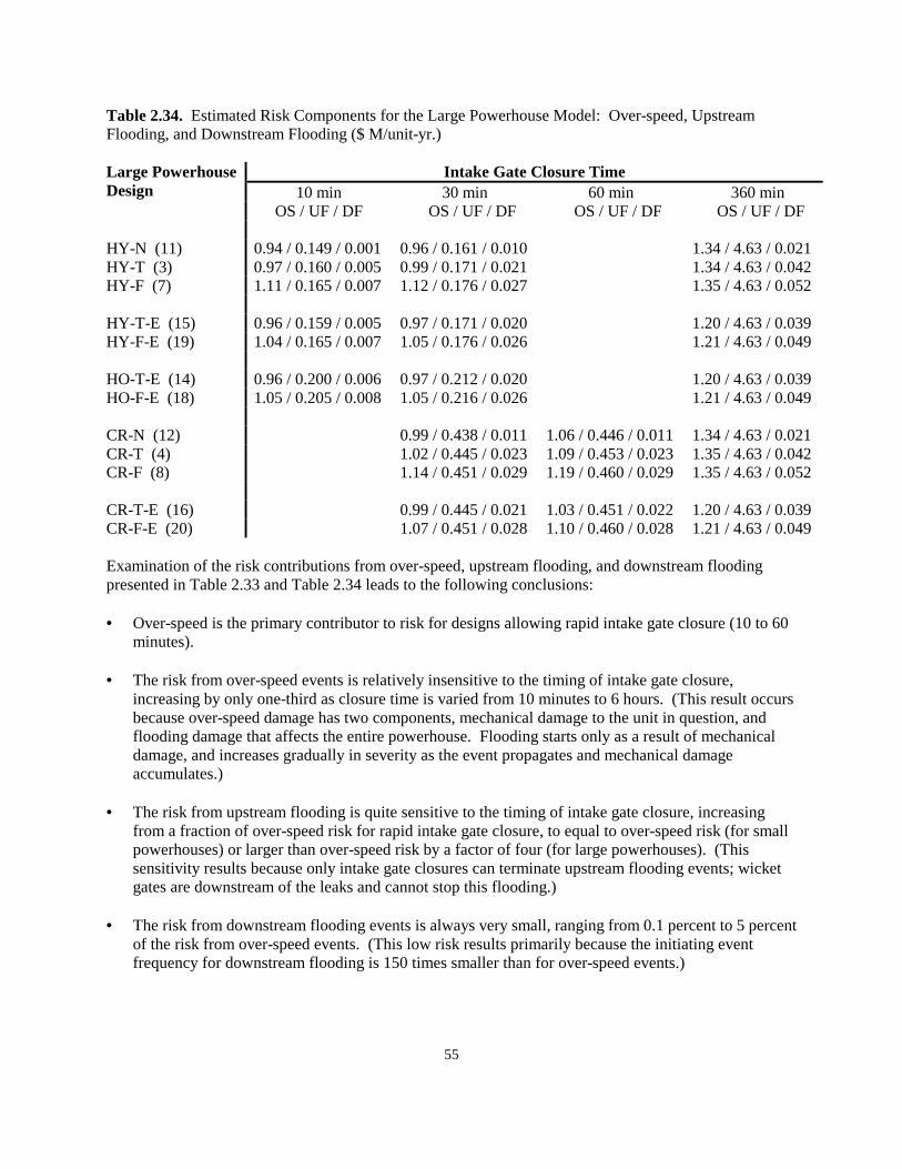
55

Table 2.34. Estimated Risk Components for the Large Powerhouse Model: Over-speed, Upstream Flooding, and Downstream Flooding ($ M/unit-yr.)

Intake Gate Closure Time 10 min 30 min 60 min 360 min

Large Powerhouse Design

OS / UF / DF OS / UF / DF OS / UF / DF OS / UF / DF HY-N (11) 0.94 / 0.149 / 0.001 0.96 / 0.161 / 0.010 1.34 / 4.63 / 0.021 HY-T (3) 0.97 / 0.160 / 0.005 0.99 / 0.171 / 0.021 1.34 / 4.63 / 0.042 HY-F (7) 1.11 / 0.165 / 0.007 1.12 / 0.176 / 0.027 1.35 / 4.63 / 0.052 HY-T-E (15) 0.96 / 0.159 / 0.005 0.97 / 0.171 / 0.020 1.20 / 4.63 / 0.039 HY-F-E (19) 1.04 / 0.165 / 0.007 1.05 / 0.176 / 0.026 1.21 / 4.63 / 0.049 HO-T-E (14) 0.96 / 0.200 / 0.006 0.97 / 0.212 / 0.020 1.20 / 4.63 / 0.039 HO-F-E (18) 1.05 / 0.205 / 0.008 1.05 / 0.216 / 0.026 1.21 / 4.63 / 0.049 CR-N (12) 0.99 / 0.438 / 0.011 1.06 / 0.446 / 0.011 1.34 / 4.63 / 0.021 CR-T (4) 1.02 / 0.445 / 0.023 1.09 / 0.453 / 0.023 1.35 / 4.63 / 0.042 CR-F (8) 1.14 / 0.451 / 0.029 1.19 / 0.460 / 0.029 1.35 / 4.63 / 0.052 CR-T-E (16) 0.99 / 0.445 / 0.021 1.03 / 0.451 / 0.022 1.20 / 4.63 / 0.039 CR-F-E (20) 1.07 / 0.451 / 0.028 1.10 / 0.460 / 0.028 1.21 / 4.63 / 0.049 Examination of the risk contributions from over-speed, upstream flooding, and downstream flooding presented in Table 2.33 and Table 2.34 leads to the following conclusions: • Over-speed is the primary contributor to risk for designs allowing rapid intake gate closure (10 to 60

minutes). • The risk from over-speed events is relatively insensitive to the timing of intake gate closure,

increasing by only one-third as closure time is varied from 10 minutes to 6 hours. (This result occurs because over-speed damage has two components, mechanical damage to the unit in question, and flooding damage that affects the entire powerhouse. Flooding starts only as a result of mechanical damage, and increases gradually in severity as the event propagates and mechanical damage accumulates.)

• The risk from upstream flooding is quite sensitive to the timing of intake gate closure, increasing

from a fraction of over-speed risk for rapid intake gate closure, to equal to over-speed risk (for small powerhouses) or larger than over-speed risk by a factor of four (for large powerhouses). (This sensitivity results because only intake gate closures can terminate upstream flooding events; wicket gates are downstream of the leaks and cannot stop this flooding.)

• The risk from downstream flooding events is always very small, ranging from 0.1 percent to 5 percent

of the risk from over-speed events. (This low risk results primarily because the initiating event frequency for downstream flooding is 150 times smaller than for over-speed events.)

56

2.4.2 Risk Uncertainty Analysis Results and Conclusions Table 2.35 presents the 5 and 95 percentile values of the distributions for each of the designs and cases analyzed, for small powerhouses. Table 2.36 presents the results for large powerhouses. Table 2.35. Uncertainty Bounds (5 and 95 percentile values) of the Estimated Total Risks for the Small Powerhouse Model ($ M/unit-yr.)

Intake Gate Closure Time 10 min 30 min 60 min 360 min

Small Powerhouse Design

5% / 95 5

5% / 95% 5% / 95% 5% / 95%

HY-N (11) 0.05 / 3.14 0.06 / 3.20 0.22 / 6.79 HY-T (3) 0.06 / 3.15 0.06 / 3.20 0.22 / 6.79 HY-F (7) 0.06 / 3.43 0.06 / 3.52 0.22 / 6.86 HY-T-E (15) 0.06 / 3.15 0.06 / 3.19 0.21 / 6.55 HY-F-E (19) 0.06 / 3.42 0.06 / 3.50 0.21 / 6.59 HO-T-E (14) 0.06 / 3.15 0.06 / 3.20 0.21 / 6.55 HO-F-E (18) 0.06 / 3.43 0.06 / 3.49 0.21 / 6.58 CR-N (12) 0.07 / 3.21 0.21 / 6.55 0.22 / 6.79 CR-T (4) 0.07 / 3.21 0.21 / 6.56 0.22 / 6.79 CR-F (8) 0.07 / 3.59 0.21 / 7.28 0.22 / 6.86 CR-T-E (16) 0.07 / 3.20 0.20 / 6.44 0.21 / 6.55 CR-F-E (20) 0.07 / 3.57 0.21 / 6.83 0.21 / 6.59

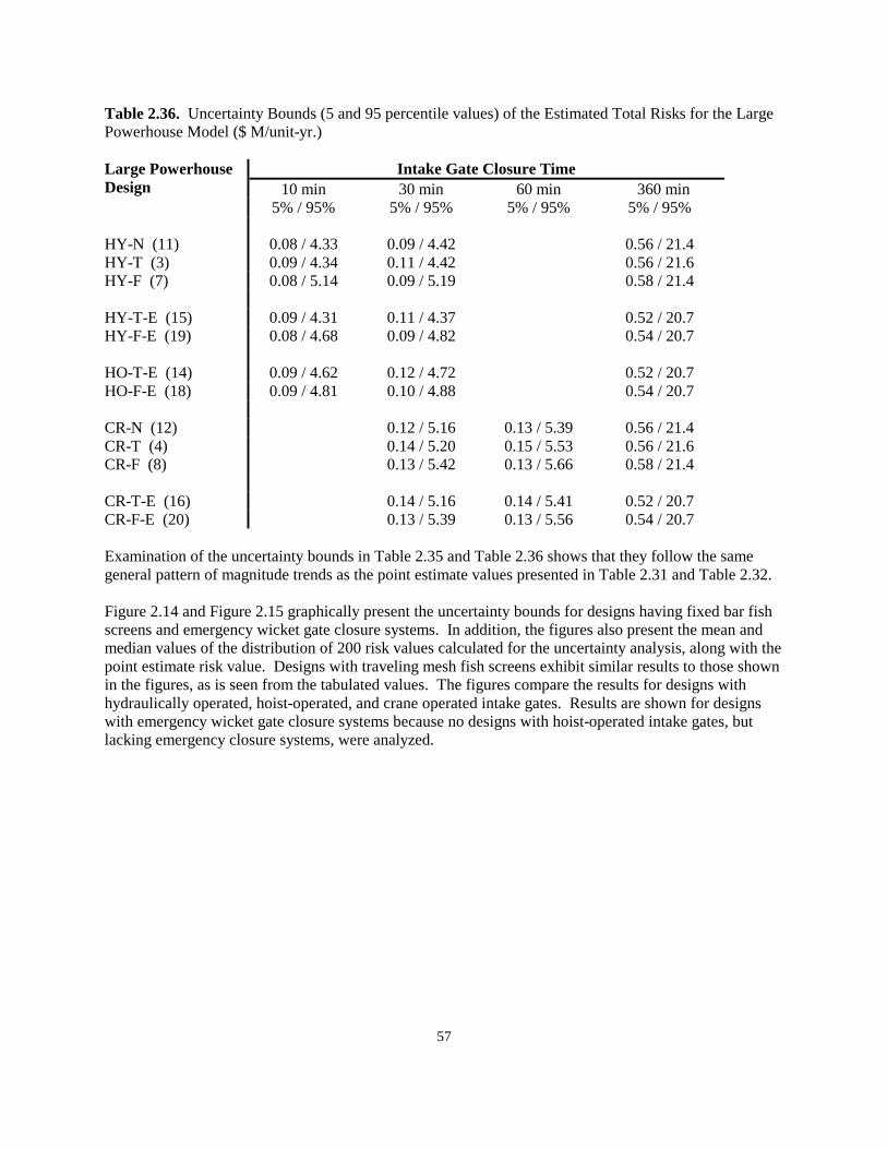
57

Table 2.36. Uncertainty Bounds (5 and 95 percentile values) of the Estimated Total Risks for the Large Powerhouse Model ($ M/unit-yr.)

Intake Gate Closure Time 10 min 30 min 60 min 360 min

Large Powerhouse Design

5% / 95% 5% / 95% 5% / 95% 5% / 95% HY-N (11) 0.08 / 4.33 0.09 / 4.42 0.56 / 21.4 HY-T (3) 0.09 / 4.34 0.11 / 4.42 0.56 / 21.6 HY-F (7) 0.08 / 5.14 0.09 / 5.19 0.58 / 21.4 HY-T-E (15) 0.09 / 4.31 0.11 / 4.37 0.52 / 20.7 HY-F-E (19) 0.08 / 4.68 0.09 / 4.82 0.54 / 20.7 HO-T-E (14) 0.09 / 4.62 0.12 / 4.72 0.52 / 20.7 HO-F-E (18) 0.09 / 4.81 0.10 / 4.88 0.54 / 20.7 CR-N (12) 0.12 / 5.16 0.13 / 5.39 0.56 / 21.4 CR-T (4) 0.14 / 5.20 0.15 / 5.53 0.56 / 21.6 CR-F (8) 0.13 / 5.42 0.13 / 5.66 0.58 / 21.4 CR-T-E (16) 0.14 / 5.16 0.14 / 5.41 0.52 / 20.7 CR-F-E (20) 0.13 / 5.39 0.13 / 5.56 0.54 / 20.7 Examination of the uncertainty bounds in Table 2.35 and Table 2.36 shows that they follow the same general pattern of magnitude trends as the point estimate values presented in Table 2.31 and Table 2.32. Figure 2.14 and Figure 2.15 graphically present the uncertainty bounds for designs having fixed bar fish screens and emergency wicket gate closure systems. In addition, the figures also present the mean and median values of the distribution of 200 risk values calculated for the uncertainty analysis, along with the point estimate risk value. Designs with traveling mesh fish screens exhibit similar results to those shown in the figures, as is seen from the tabulated values. The figures compare the results for designs with hydraulically operated, hoist-operated, and crane operated intake gates. Results are shown for designs with emergency wicket gate closure systems because no designs with hoist-operated intake gates, but lacking emergency closure systems, were analyzed.

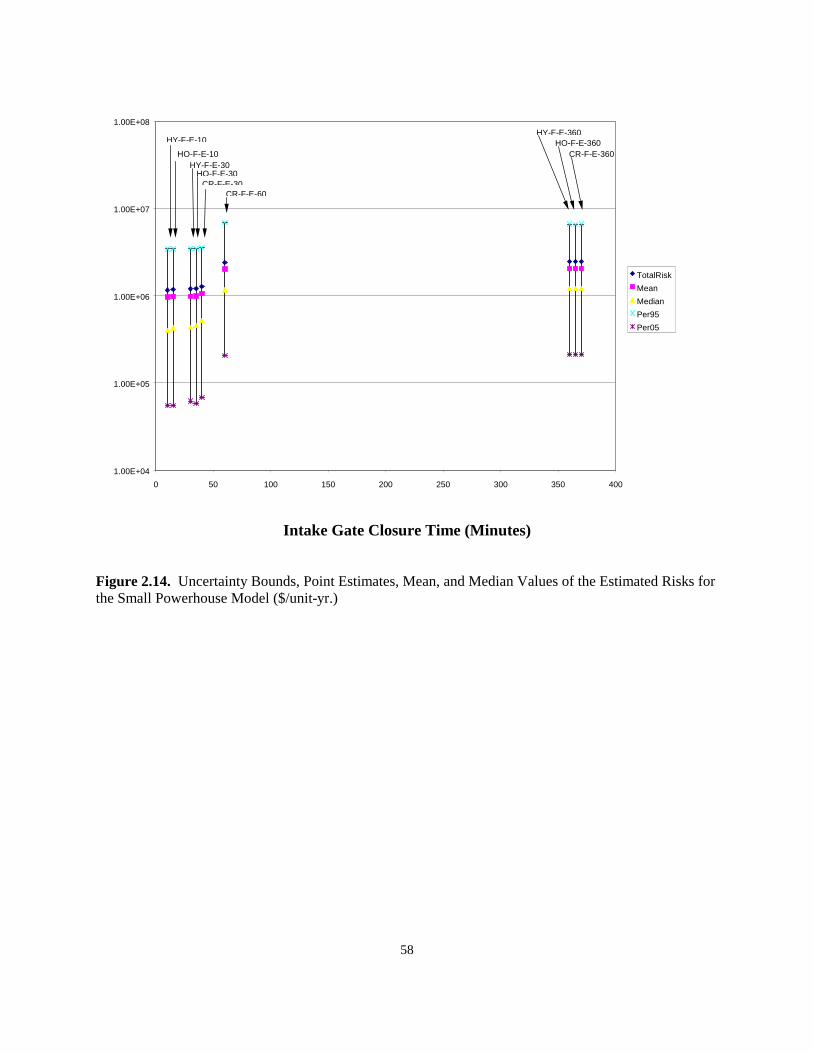
58

Intake Gate Closure Time (Minutes)

Figure 2.14. Uncertainty Bounds, Point Estimates, Mean, and Median Values of the Estimated Risks for the Small Powerhouse Model ($/unit-yr.)

1.00E+04

1.00E+05

1.00E+06

1.00E+07

1.00E+08

0 50 100 150 200 250 300 350 400

TotalRisk

Mean

Median

Per95

Per05

HY-F-E-10

HO-F-E-10

CR-F-E-30

HY-F-E-30HO-F-E-30

CR-F-E-60

HY-F-E-360HO-F-E-360

CR-F-E-360

59

Intake Gate Closure Time (Minutes)

Figure 2.15. Uncertainty Bounds, Point Estimates, Mean, and Median Values of the Estimated Risks for the Large Powerhouse Model ($/unit-yr.) Examination of the risk values presented in Figure 2.14 and Figure 2.15 yields the following conclusions: • Roughly a factor of 50 exists between the upper and lower uncertainty bounds. For designs capable

of intake gate closure at short times, the factor ranges between 45 and 65. For designs requiring long times for intake gate closure, the factor ranges between 30 and 40. (This uncertainty range results from uncertainties in the basic event database.)

• Median values of the sampled distributions are well centered between the uncertainty bounds, as they

should be. Mean values of the sampled distributions exceed median values by a factor of about 2. • Point estimate risk values are acceptably close to the mean values of the sampled risk distributions.

Agreement is better for the small powerhouse model than for the large model. (General agreement is expected because the point estimate values used for individual component failure probabilities were the mean values of the probability distributions for the components.)

1.00E+04

1.00E+05

1.00E+06

1.00E+07

1.00E+08

0 50 100 150 200 250 300 350 400

TotalRisk

Mean

Median

Per95

Per05

HY-F-E-10

HO-F-E-10

CR-F-E-30

HY-F-E-30HO-F-E-30

CR-F-E-60

HY-F-E-360HO-F-E-360

CR-F-E-360

60

3 Uncertainty Analysis Methodology The uncertainty analysis employed in this study is a form of Monte Carlo simulation analysis using Latin Hypercube Sampling. The methodology used in this analysis is explained in this section, along with the distribution functions used to represent the basic event probabilities in the database. The results of the uncertainty analysis are shown in the various sections presenting intermediate and final results of the analysis.

3.1 Monte Carlo Simulation Monte Carlo simulation consists of making repeated evaluations of a function (i.e. the risk for a given design) using values selected at random from the uncertainty distributions of the input parameters. For each iteration of the Monte Carlo run, each input parameter is randomly sampled from its associated distribution, and the function is evaluated. After many repetitions, a distribution of function values results that can be sorted and analyzed to obtain mean and median values, and 5th and 95th percentiles. For each of the basic event parameters used in this analysis, a distribution function centered about a point estimate value is used to represent the uncertainty of the parameter. The distribution function provides the probability that the parameter may have any of the values within its assigned uncertainty bounds. Thus, uncertainties and distribution functions are assigned to all of the basic data used in the analysis. These data include failure frequencies, probabilities of failure on demand, estimates of the costs to repair damage states, and estimates of costs of proposed system modifications. The Monte Carlo analysis sampled all of the distribution functions randomly during each iteration in order to develop a distribution of results that would represent the result uncertainty.

3.2 Latin Hypercube Sampling Latin Hypercube Sampling is a method that reduces the number of iterations necessary to obtain an accurate measure of the result uncertainty. In Latin Hypercube Sampling, the distribution functions are sampled at specific increments, and then the samples are randomized. This process ensures a complete span of the distribution function values with fewer samples than for purely random sampling, while maintaining randomized results. This analysis used 200 samples of each distribution function. Thus, after the calculational results were sorted by size, and the smallest 10 and largest 10 results were set aside, the span of the remaining results defined the 5th and 95th percentile confidence limits of the result. The Latin Hypercube method of selecting the distribution function samples is as follows. Each distribution function is integrated into a cumulative distribution function spanning the probability range from zero to 1.0. This range is then divided into (200) equal parts, and the inverse of the cumulative distribution function is used to determine the specific value of the parameter that corresponds to each of the parts. These are the samples. These carefully selected samples are then randomized, yielding the effect of random sampling that completely spans the distribution, but with many fewer samples than would be required if the sampling were completely random.

61

3.3 Distribution Functions Used Several different distribution functions were used to represent the input data in this study. Fitted gamma functions were used to represent the parameters for which survey and expert elicitation data were combined by Bayesian updating. Log-normal distribution functions were used to represent parameters for which COE members supplied screening value estimates, and also for generic data values obtained from IEEE 500, the NERC/GADS compilations, and from NRC Regulatory Guides. Error factors for the generic values were taken from the tabulations – most had an error factor of 10, except the GADS data, that had an error factor of 100. Screening values were assigned an error factor of 10. A 20 percent uniform uncertainty was assigned to probability values in the flooding matrixes based on discussions with COE personnel and a review of the possible flooding mechanisms. Because for each time step the probability values in the flooding matrixes need to sum to 1.0, after selection of the random values for these probabilities they were normalized by dividing by their sum at each time step. Uncertainties were assigned to all seven of the inputs to the damage state cost contribution. As was discussed in Section 3.3.2.1 addressing construction costs, an analysis was performed of the percentage difference between COE cost estimates and low bids for construction work performed for the COE between 1964 and 1994. The data were found to conform to a normal distribution with a mean of –14.5 percent and a standard deviation of 17 percent. These values were incorporated into the uncertainty analysis by assuming a normal distribution function for the construction cost estimates having a mean value 14.5 percent smaller than the COE estimate, and a 17 percent standard deviation. Uniform distributions of 5 percent were assumed, based on COE estimates, for construction time-to-repair, environmental time-to-repair, unit time-out-of-service, and for environmental costs. The lost opportunity costs depend on the average annual energy produced by each unit (AE), the cumulative value of energy for each unit (CE), and the time-out-of-service for each unit. The uncertainty in AE was addressed using a histogram based on a 50-year history of AE values. The histogram divided each year into 15 time periods during which an event might happen. Separate analyses were carried out for small (Lower Granite data) and large (The Dalles data) facilities. Latin Hypercube sampling of AE values was carried out by sampling from the time-based histogram. The cumulative value of energy, CE, depends on estimates of future power costs that were obtained from the Bonneville Power Administration (BPA). The BPA provided estimates of projected average system costs for the period 1996-2014 that included 5th and 95th percentile uncertainty estimates. These estimates were fitted to composite log-normal distributions with these uncertainties, and Latin Hypercube Sampling was performed for these fitted distributions. The uncertainty analysis for the economic evaluation of proposed modifications paralleled the methods used for the construction cost evaluation of damage states. For each of the cost categories, including capital costs, annual maintenance costs and benefits, and periodic maintenance costs, a normal distribution function was assumed with a mean value 14.5 percent smaller than the COE estimate, and a 17 percent standard deviation. This assumption incorporated the historical experience that job bid values were somewhat less than COE estimates. For the construction period estimates, a 5 percent uniform distribution was assumed, as was done for the time estimates used in the damage state evaluation.

62

For the convenience of the reader the results of the uncertainty analysis are presented along with the results of point estimate calculations. In Section 2.2.4 Event Frequency Profiles, Figure 2.6 presents uncertainty bounds compared with point estimates of event frequencies. In Section 2.3.3 Economic Consequence Analysis, Figure 2.11, Figure 2.12, and Figure 2.13 present uncertainty bounds compared with point estimates of expected costs of flooding. In Section 2.4 Risk Analysis Results and Conclusions, Table 2.35, Table 2.36, Figure 2.13, and Figure 2.14 present uncertainty bounds compared with point estimates of total risks for both small and large powerhouse models. In the following Section 4 Benefit-Cost Analysis, Table 4.3, Table 4.4, Figure 4.1, and Figure 4.2 present uncertainty bounds compared with point estimates of net present value, and of benefit cost ratio for proposed powerhouse modifications.

4 Benefit-Cost Analysis Modifications proposed for the intake gate configurations of hydroelectric stations on the Snake and Columbia rivers in eastern Washington State would speed intake gate closure, thus reducing the risks of station damage during non-routine shutdowns. This economic analysis compares benefits of the proposed modifications with the costs of their implementation. The stations as they exist presently, and the proposed modifications, correspond to design variants analyzed in the risk analysis portion of this study. Thus, the risk reduction achievable from each of the proposed modifications is simply the difference between the risks already calculated for the existing and modified configurations. The stations, their existing configurations, and the proposed modified configurations are shown in Table 4.1. Table 4.1. Modifications Proposed for Hydroelectric Station Intake Gate Operating Systems

Existing Powerhouse Station Name Existing Design

Proposed Modified Designs

HY-F-E-10-large McNary HY-F-E-360-

large HO-F-E-10-large

HY-T-E-10-small Lower Monumental

HY-T-E-360-small HO-T-E-10-small

HY-F-E-10-small Little Goose/

Lower Granite HY-F-E-360-small HO-F-E-10-small

4.1 Methodology Two measures of the economic effectiveness of these modifications were evaluated. The primary measure used to evaluate government projects is the net present value (NPV), i.e. the discounted dollar value of future net benefits (benefits – costs). The preferred supplemental measure is the benefit/cost ratio (BC), i.e. the discounted dollar value of future benefits, divided by the discounted dollar value of implementation, operations, and maintenance costs. Both of these measures were evaluated. The present value calculations assume that risk reduction benefits and maintenance costs occur annually at the midpoint of each year for 25 years. Implementation costs are assumed to occur monthly at the

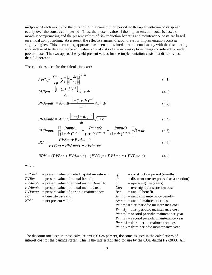
63

midpoint of each month for the duration of the construction period, with implementation costs spread evenly over the construction period. Thus, the present value of the implementation costs is based on monthly compounding and the present values of risk reduction benefits and maintenance costs are based on annual compounding. As a result, the effective annual discount rate for implementation costs is slightly higher. This discounting approach has been maintained to retain consistency with the discounting approach used to determine the equivalent annual risks of the various options being considered for each powerhouse. The two approaches yield present values for the implementation costs that differ by less than 0.5 percent. The equations used for the calculations are:

)5.(

1 121

−

∑

+=

cpcp dr

cp

ConPVCap (4.1)

[ ]dr

dr

drPVBen

ol

++−=−

1)1(1

(4.2)

[ ]dr

dr

drAmntbPVAmntb

ol

++−=−

1)1(1

(4.3)

[ ]dr

dr

drAmntcPVAmntc

ol

++−=−

1)1(1

(4.4)

drdr

Pmntc

dr

Pmntc

dr

PmntcPVPmntc

yPmntyPmntyPmnt+

+

++

++

= 1)1(

3

)1(

2

)1(

1321 (4.5)

PVPmntcPVAmntcPVCap

PVAmntbPVBenBC

+++= (4.6)

)()( PVPmntcPVAmntcPVCapPVAmntbPVBenNPV ++−+= (4.7)

where PVCaP = present value of initial capital investment cp = construction period (months) PVBen = present value of annual benefit dr = discount rate (expressed as a fraction) PVAmnb = present value of annual maint. Benefits ol = operating life (years) PVAmntc = present value of annual maint. Costs Con = overnight construction costs PVPmntc = present value of periodic maintenance Ben = annual benefit BC = benefit/cost ratio Amntb = annual maintenance benefits NPV = net present value Amntc = annual maintenance cost Pmntc1 = first periodic maintenance cost Pmnt1y = first periodic maintenance cost

Pmntc2 = second periodic maintenance year Pmnt2y = second periodic maintenance year Pmntc3 = third period maintenance cost Pmnt3y = third periodic maintenance year The discount rate used in these calculations is 6.625 percent, the same as used in the calculations of interest cost for the damage states. This is the rate established for use by the COE during FY-2000. All

64

costs and benefits were discounted to the end of the construction period. Thus, the present value of implementation (construction) costs includes interest during construction. No specific assumptions were made regarding when the construction projects would begin or end, just the length of the construction period. With all costs and benefits assumed to escalate at the same rate, the implementation date does not affect the NPV or BC calculations. The inputs for calculations were estimated by the COE and provided to PNNL. The risk reduction benefits were obtained by subtracting the risks for 10-minute closure from the risks for 360-minute closure for each powerhouse evaluated, and then multiplying by the number of units appropriate for each powerhouse (14 for McNary and 6 for the other 3). Periodic maintenance was estimated for the hydraulic modification as a single effort at 25 years, and for the hoist systems as 3 efforts at 8, 16, and 24 years. The inputs to the calculations are listed in Table 4.2. Table 4.2. Values Input into the Calculations of Net Present Value and Benefit/Cost Ratio ($ Million)

Benefits Costs Annual Risk Reduction

Annual Maintenance

Construction “Overnight”

Annual Maintenance

Periodic Maintenance

HY 65.4 0.026 46.9 0.009 6.30 @ 25 yrs. McNary HO 64.8 0.026 20.1 0.039 2.57 @ 8, 16, &

24 yrs.

HY 7.87 0.011 8.54 0.0009 0.61 @ 25 yrs. Lower Monumental HO 7.80 0.011 7.01 0.017 1.10 @ 8, 16, &

24 yrs.

HY 7.71 0.011 20.3 0.004 2.70 @ 25 yrs. Little Goose/ Lower Granite

HO 7.64 0.011 7.01 0.017 1.10 @ 8, 16, & 24 yrs.

4.2 Benefit-Cost Results and Conclusions The results of the economic analysis are presented graphically in Figure 4.1 and Figure 4.2, and listed in Table 4.3 and Table 4.4. The graphical display facilitates evaluation of the spread of values, and the tabular display provides precise values.

65

Net Present Value

$1,000,000

$10,000,000

$100,000,000

$1,000,000,000

$10,000,000,000

Best Est.

Median

Mean

HY HO HY HO HY HO McNARY LOWER MONUMENTAL L. GOOSE / L. GRANITE Figure 4.1. Point Estimates and Uncertainty Bounds of the Estimated Net Present Value for the Proposed Powerhouse Modifications (Note: The lower uncertainty bounds are negative (and thus offscale) for all but one case.)

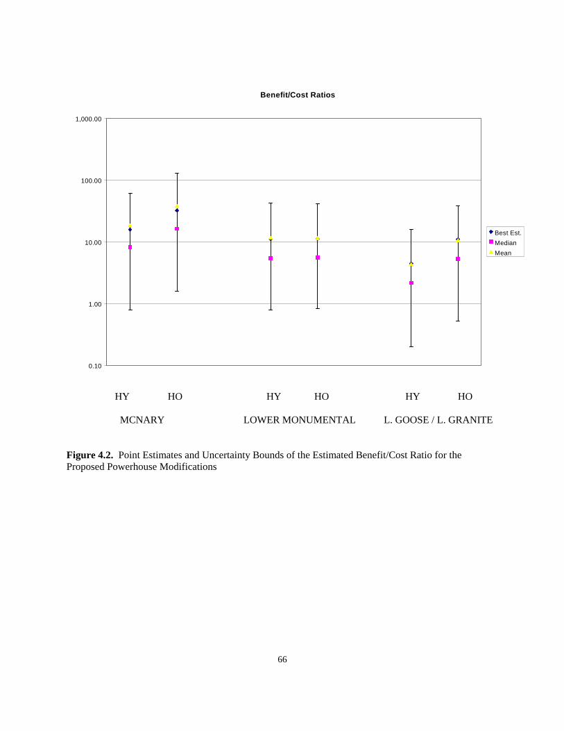
66

Benefit/Cost Ratios

0.10

1.00

10.00

100.00

1,000.00

Best Est.

Median

Mean

HY HO HY HO HY HO MCNARY LOWER MONUMENTAL L. GOOSE / L. GRANITE Figure 4.2. Point Estimates and Uncertainty Bounds of the Estimated Benefit/Cost Ratio for the Proposed Powerhouse Modifications

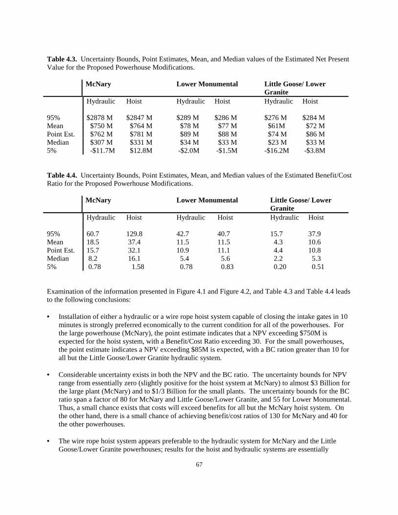
67

Table 4.3. Uncertainty Bounds, Point Estimates, Mean, and Median values of the Estimated Net Present Value for the Proposed Powerhouse Modifications. McNary Lower Monumental Little Goose/ Lower

Granite Hydraulic Hoist Hydraulic Hoist Hydraulic Hoist 95% $2878 M $2847 M $289 M $286 M $276 M $284 M Mean $750 M $764 M $78 M $77 M $61M $72 M Point Est. $762 M $781 M $89 M $88 M $74 M $86 M Median $307 M $331 M $34 M $33 M $23 M $33 M 5% -$11.7M $12.8M -$2.0M -$1.5M -$16.2M -$3.8M Table 4.4. Uncertainty Bounds, Point Estimates, Mean, and Median values of the Estimated Benefit/Cost Ratio for the Proposed Powerhouse Modifications. McNary Lower Monumental Little Goose/ Lower

Granite Hydraulic Hoist Hydraulic Hoist Hydraulic Hoist 95% 60.7 129.8 42.7 40.7 15.7 37.9 Mean 18.5 37.4 11.5 11.5 4.3 10.6 Point Est. 15.7 32.1 10.9 11.1 4.4 10.8 Median 8.2 16.1 5.4 5.6 2.2 5.3 5% 0.78 1.58 0.78 0.83 0.20 0.51 Examination of the information presented in Figure 4.1 and Figure 4.2, and Table 4.3 and Table 4.4 leads to the following conclusions: • Installation of either a hydraulic or a wire rope hoist system capable of closing the intake gates in 10

minutes is strongly preferred economically to the current condition for all of the powerhouses. For the large powerhouse (McNary), the point estimate indicates that a NPV exceeding $750M is expected for the hoist system, with a Benefit/Cost Ratio exceeding 30. For the small powerhouses, the point estimate indicates a NPV exceeding $85M is expected, with a BC ration greater than 10 for all but the Little Goose/Lower Granite hydraulic system.

• Considerable uncertainty exists in both the NPV and the BC ratio. The uncertainty bounds for NPV

range from essentially zero (slightly positive for the hoist system at McNary) to almost $3 Billion for the large plant (McNary) and to $1/3 Billion for the small plants. The uncertainty bounds for the BC ratio span a factor of 80 for McNary and Little Goose/Lower Granite, and 55 for Lower Monumental. Thus, a small chance exists that costs will exceed benefits for all but the McNary hoist system. On the other hand, there is a small chance of achieving benefit/cost ratios of 130 for McNary and 40 for the other powerhouses.

• The wire rope hoist system appears preferable to the hydraulic system for McNary and the Little

Goose/Lower Granite powerhouses; results for the hoist and hydraulic systems are essentially

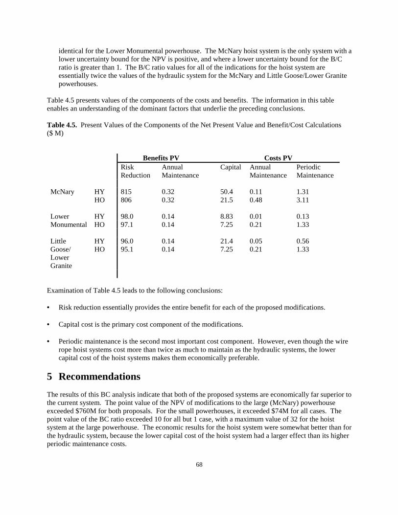
68

identical for the Lower Monumental powerhouse. The McNary hoist system is the only system with a lower uncertainty bound for the NPV is positive, and where a lower uncertainty bound for the B/C ratio is greater than 1. The B/C ratio values for all of the indications for the hoist system are essentially twice the values of the hydraulic system for the McNary and Little Goose/Lower Granite powerhouses.

Table 4.5 presents values of the components of the costs and benefits. The information in this table enables an understanding of the dominant factors that underlie the preceding conclusions. Table 4.5. Present Values of the Components of the Net Present Value and Benefit/Cost Calculations ($ M)

Benefits PV Costs PV Risk Reduction

Annual Maintenance

Capital Annual Maintenance

Periodic Maintenance

HY 815 0.32 50.4 0.11 1.31 McNary HO 806 0.32 21.5 0.48 3.11

HY 98.0 0.14 8.83 0.01 0.13 Lower

Monumental HO 97.1 0.14 7.25 0.21 1.33

HY 96.0 0.14 21.4 0.05 0.56 Little Goose/ Lower Granite

HO 95.1 0.14 7.25 0.21 1.33

Examination of Table 4.5 leads to the following conclusions: • Risk reduction essentially provides the entire benefit for each of the proposed modifications. • Capital cost is the primary cost component of the modifications. • Periodic maintenance is the second most important cost component. However, even though the wire

rope hoist systems cost more than twice as much to maintain as the hydraulic systems, the lower capital cost of the hoist systems makes them economically preferable.

5 Recommendations The results of this BC analysis indicate that both of the proposed systems are economically far superior to the current system. The point value of the NPV of modifications to the large (McNary) powerhouse exceeded $760M for both proposals. For the small powerhouses, it exceeded $74M for all cases. The point value of the BC ratio exceeded 10 for all but 1 case, with a maximum value of 32 for the hoist system at the large powerhouse. The economic results for the hoist system were somewhat better than for the hydraulic system, because the lower capital cost of the hoist system had a larger effect than its higher periodic maintenance costs.

69

Considerable uncertainty was found in all point estimate values, due to uncertainties in the basic event failure rate data. For the BC analysis, the 5 percent lower uncertainty bound indicates a small chance exists that costs will exceed benefits for all but the hoist system at the large (McNary) powerhouse. On the other hand, a small chance also exists of achieving benefit/cost ratios of 130 for McNary powerhouse and of 40 for the other powerhouses. Based on the results of this study, it is recommended that upgrading the intake gate operators to allow closure within 10 minutes is a cost effective solution at the Lower Granite, Little Goose, Lower Monumental, and McNary Dams. Based on the cost estimates and maintenance costs for the two competing solutions, the wire rope hoist is the most cost-effective approach to meet the closure criteria at these powerhouses. The results for these powerhouses do not necessarily translate to other plants in the COE. Each plant should be examined individually and a recommendation presented based on the specifics of an individual plant. However, it can be asserted that intake gate closure within 10 minutes is a supportable design goal. At plants where a minimal investment is required to achieve 10-minute closure, a decision to upgrade equipment easily can be supported.

70

References Curley, G.M. 1994. Hydropower Turbine/Generator Cause Code Summaries, 1982-1993. U.S. Army Corps of Engineers, Portland, OR. Idaho National Engineering Laboratory (INEL) 1996. Saphire Reference Manual. Idaho National Engineering Laboratory, Idaho Falls, ID. Institute of Electrical and Electronics Engineers (IEEE) 1983. Guide to the Collection and Presentation of Electrical, Electronic, Sensing Component, and Mechanical Equipment Reliability Data for Nuclear Power Generating Stations. Std 500-1984, Institute of Electrical and Electronics Engineers. Lewis, E.E. 1987. Introduction to Reliability Engineering. John Wiley & Sons, Inc., New York. McCormick, Norman J. 1981. Reliability and Risk Analysis. Academic Press, Inc., Orlando, FL. U.S. Nuclear Regulatory Commission (NRC) 1985. Probabilistic Safety Analysis Procedures Guide. U.S. Nuclear Regulatory Commission, Washington, D.C. U.S. Nuclear Regulatory Commission (NRC) 1987. Accident Sequence Evaluation Program-Human Reliability Analysis Procedures Guide. NUREG/CR-4772. U.S. Nuclear Regulatory Commission, Washington, D.C. U.S. Nuclear Regulatory Commission (NRC) 1981. Fault Tree Handbook. NUREG-0492. U.S. Nuclear Regulatory Commission, Washington, D.C. Wheeler et al. 1989. Analysis of Core Damage Frequency from Internal Events: Expert Judgment Elicitation. NU-REG/CR-4550, Vol. 2, U.S. Nuclear Regulatory Commission.

Appendix A

Basic Event Failure Data

A-1

Appendix A. Basic Event Failure Data The following table presents the database of basic event failures used in the time based reliability analysis, specifically in the calculations of the frequency profiles that describe the annual probability of over-speed, upstream flooding and downstream flooding events. Most of the data on powerhouse components were gathered as failure rates (per year) and, consequently, they are presented in this form. The probability of failure on demand is used in calculations involving components in the wicket gate and intake gate systems. For operating components, calculation of the demand failure probability requires multiplication of the component failure rate, λ, by the time necessary to respond to the problem situation. This time is referred to as the mission time in the following table. In most cases the mission time was conservatively assumed to be 12 hours. This figure is referred to as Calculation Type 2 in the table. Calculation Type 1 involved using the demand failure directly (when it could be obtained directly, usually from tabulations of generic data). For standby components that are not operating continuously, calculation of the demand failure probability requires use of an exposure time, τ, that is the time between operations that demonstrate the operability of the component. Use of the exposure time allows for the possibility the component might degrade or be damaged while on standby. The demand failure probability is λτ /2, where τ/2 represents the average time during the exposure when such a failure might occur. This is referred to as Calculation Type 6 in the table. A distribution function was associated with every entry in the database, to enable uncertainty analysis calculations that sampled randomly from the distribution functions and developed a distribution of results bounding the point estimate results. Gamma functions were used for data that combined survey and expert judgment workshop evaluations, because such functions are the standard ones used in the Bayesian updating process that combines data from different sources. Gamma functions are coded in the table as distribution type 3. The table also presents values of the associated Distribution Parameter that is related to the spread of the distribution. The values presented in the table are those of the parameter b1 in Equation 3.7, namely, the square of the mean divided by the variance. Data obtained from generic tabulations were mostly in the form of mean values and error factors associated with log normal distribution functions. Log normal distributions are coded as type 2 in the table. The distribution parameter listed in the table for log normal distributions is the error factor, that is 1/λ times the 95 percent upper confidence bound of the distribution.

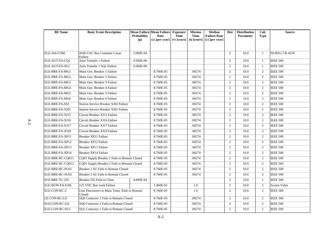
A-2

BE Name Basic Event Description Mean Failure Probability

(p)

Mean Failure Rate

(λ) [per year]

Exposure Time

(τ) [years]

Mission Time

(t) [years]

Median Failure Rate (λ) [per year]

Dist Distribution Parameter

Calc Type

Source

ELE-416-COM 4160 VAC Bus Common Cause Failure

5.000E-04 2 10.0 1 NUREG CR-4550

ELE-AUT-FA-CQ1 Auto Transfer 1 Failure 4.560E-06 2 10.0 1 IEEE 500

ELE-AUT-FA-SU1 Auto Transfer 1 SQ1 Failure 4.560E-06 2 10.0 1 IEEE 500

ELE-BRE-FA-MG1 Main Gen. Breaker 1 Failure 8.760E-05 .00274 2 10.0 2 IEEE 500

ELE-BRE-FA-MG2 Main Gen. Breaker 2 Failure 8.760E-05 .00274 2 10.0 2 IEEE 500

ELE-BRE-FA-MG3 Main Gen. Breaker 3 Failure 8.760E-05 .00274 2 10.0 2 IEEE 500

ELE-BRE-FA-MG4 Main Gen. Breaker 4 Failure 8.760E-05 .00274 2 10.0 2 IEEE 500

ELE-BRE-FA-MG5 Main Gen. Breaker 5 Failure 8.760E-05 .00274 2 10.0 2 IEEE 500

ELE-BRE-FA-MG6 Main Gen. Breaker 6 Failure 8.760E-05 .00274 2 10.0 2 IEEE 500

ELE-BRE-FA-SS2 Station Service Breaker XJ02 Failure 8.760E-05 .00274 2 10.0 2 IEEE 500

ELE-BRE-FA-XJ01 Station Service Breaker XJ01 Failure 8.760E-05 .00274 2 10.0 2 IEEE 500

ELE-BRE-FA-XJ15 Circuit Breaker XJ15 Failure 8.760E-05 .00274 2 10.0 2 IEEE 500

ELE-BRE-FA-XJ16 Circuit Breaker XJ16 Failure 8.760E-05 .00274 2 10.0 2 IEEE 500

ELE-BRE-FA-XJ17 Circuit Breaker XJ17 Failure 8.760E-05 .00274 2 10.0 2 IEEE 500

ELE-BRE-FA-XJ18 Circuit Breaker XJ18 Failure 8.760E-05 .00274 2 10.0 2 IEEE 500

ELE-BRE-FA-XP11 Breaker XP11 Failure 8.760E-05 .00274 2 10.0 2 IEEE 500

ELE-BRE-FA-XP12 Breaker XP12 Failure 8.760E-05 .00274 2 10.0 2 IEEE 500

ELE-BRE-FA-XP13 Breaker XP11 Failure 8.760E-05 .00274 2 10.0 2 IEEE 500

ELE-BRE-FA-XP14 Breaker XP14 Failure 8.760E-05 .00274 2 10.0 2 IEEE 500

ELE-BRE-RC-CQ011 CQ01 Supply Breaker 1 Fails to Remain Closed 8.760E-05 .00274 2 10.0 2 IEEE 500

ELE-BRE-RC-CQ012 CQ01 Supply Breaker 2 Fails to Remain Closed 8.760E-05 .00274 2 10.0 2 IEEE 500

ELE-BRE-RC-SU01 Breaker 1 SU Fails to Remain Closed 8.760E-05 .00274 2 10.0 2 IEEE 500

ELE-BRE-RC-SU02 Breaker 2 SU Fails to Remain Closed 8.760E-05 .00274 2 10.0 2 IEEE 500

ELE-BRE-TC-ZJ5 Breaker ZJ5 Fails to Close 4.000E-04 2 10.0 1 IEEE 500

ELE-BUW-FA-FAIL 125 VDC Bus work Failure 1.060E-02 1.0 2 10.0 2 Screen Value

ELE-CON-RC-2 Line Disconnect to Main Trans. Fails to Remain Closed

8.760E-05 1.0 2 10.0 2 IEEE 500

LE-CON-RC-LI1 SQ0 Contactor 1 Fails to Remain Closed 8.760E-05 .00274 2 10.0 2 IEEE 500

ELE-CON-RC-LI2 SQ0 Contactor 2 Fails to Remain Closed 8.760E-05 .00274 2 10.0 2 IEEE 500

ELE-CON-RC-SU1 SQ1 Contactor 1 Fails to Remain Closed 8.760E-05 .00274 2 10.0 2 IEEE 500

A-2

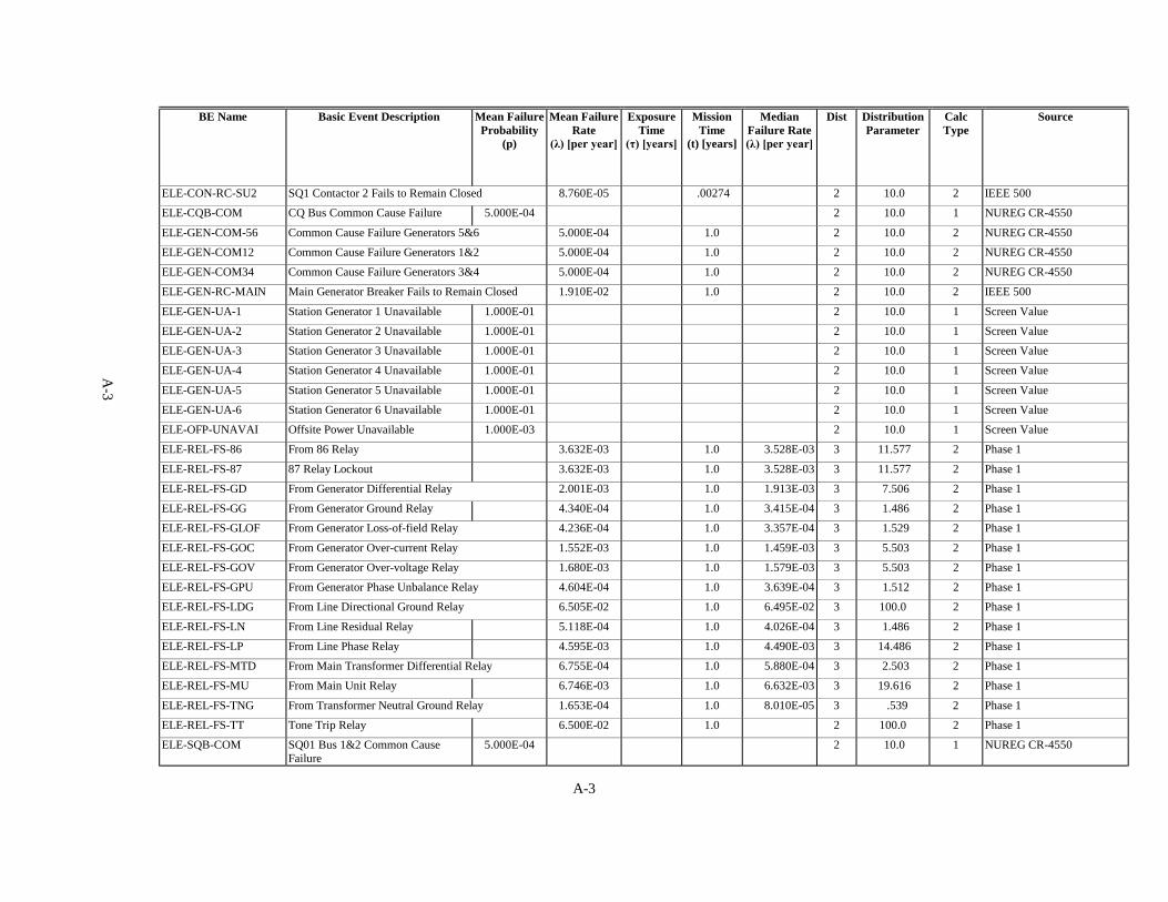
A-3

BE Name Basic Event Description Mean Failure Probability

(p)

Mean Failure Rate

(λ) [per year]

Exposure Time

(τ) [years]

Mission Time

(t) [years]

Median Failure Rate (λ) [per year]

Dist Distribution Parameter

Calc Type

Source

ELE-CON-RC-SU2 SQ1 Contactor 2 Fails to Remain Closed 8.760E-05 .00274 2 10.0 2 IEEE 500

ELE-CQB-COM CQ Bus Common Cause Failure 5.000E-04 2 10.0 1 NUREG CR-4550

ELE-GEN-COM-56 Common Cause Failure Generators 5&6 5.000E-04 1.0 2 10.0 2 NUREG CR-4550

ELE-GEN-COM12 Common Cause Failure Generators 1&2 5.000E-04 1.0 2 10.0 2 NUREG CR-4550

ELE-GEN-COM34 Common Cause Failure Generators 3&4 5.000E-04 1.0 2 10.0 2 NUREG CR-4550

ELE-GEN-RC-MAIN Main Generator Breaker Fails to Remain Closed 1.910E-02 1.0 2 10.0 2 IEEE 500

ELE-GEN-UA-1 Station Generator 1 Unavailable 1.000E-01 2 10.0 1 Screen Value

ELE-GEN-UA-2 Station Generator 2 Unavailable 1.000E-01 2 10.0 1 Screen Value

ELE-GEN-UA-3 Station Generator 3 Unavailable 1.000E-01 2 10.0 1 Screen Value

ELE-GEN-UA-4 Station Generator 4 Unavailable 1.000E-01 2 10.0 1 Screen Value

ELE-GEN-UA-5 Station Generator 5 Unavailable 1.000E-01 2 10.0 1 Screen Value

ELE-GEN-UA-6 Station Generator 6 Unavailable 1.000E-01 2 10.0 1 Screen Value

ELE-OFP-UNAVAI Offsite Power Unavailable 1.000E-03 2 10.0 1 Screen Value

ELE-REL-FS-86 From 86 Relay 3.632E-03 1.0 3.528E-03 3 11.577 2 Phase 1

ELE-REL-FS-87 87 Relay Lockout 3.632E-03 1.0 3.528E-03 3 11.577 2 Phase 1

ELE-REL-FS-GD From Generator Differential Relay 2.001E-03 1.0 1.913E-03 3 7.506 2 Phase 1

ELE-REL-FS-GG From Generator Ground Relay 4.340E-04 1.0 3.415E-04 3 1.486 2 Phase 1

ELE-REL-FS-GLOF From Generator Loss-of-field Relay 4.236E-04 1.0 3.357E-04 3 1.529 2 Phase 1

ELE-REL-FS-GOC From Generator Over-current Relay 1.552E-03 1.0 1.459E-03 3 5.503 2 Phase 1

ELE-REL-FS-GOV From Generator Over-voltage Relay 1.680E-03 1.0 1.579E-03 3 5.503 2 Phase 1

ELE-REL-FS-GPU From Generator Phase Unbalance Relay 4.604E-04 1.0 3.639E-04 3 1.512 2 Phase 1

ELE-REL-FS-LDG From Line Directional Ground Relay 6.505E-02 1.0 6.495E-02 3 100.0 2 Phase 1

ELE-REL-FS-LN From Line Residual Relay 5.118E-04 1.0 4.026E-04 3 1.486 2 Phase 1

ELE-REL-FS-LP From Line Phase Relay 4.595E-03 1.0 4.490E-03 3 14.486 2 Phase 1

ELE-REL-FS-MTD From Main Transformer Differential Relay 6.755E-04 1.0 5.880E-04 3 2.503 2 Phase 1

ELE-REL-FS-MU From Main Unit Relay 6.746E-03 1.0 6.632E-03 3 19.616 2 Phase 1

ELE-REL-FS-TNG From Transformer Neutral Ground Relay 1.653E-04 1.0 8.010E-05 3 .539 2 Phase 1

ELE-REL-FS-TT Tone Trip Relay 6.500E-02 1.0 2 100.0 2 Phase 1

ELE-SQB-COM SQ01 Bus 1&2 Common Cause Failure

5.000E-04 2 10.0 1 NUREG CR-4550

A-3

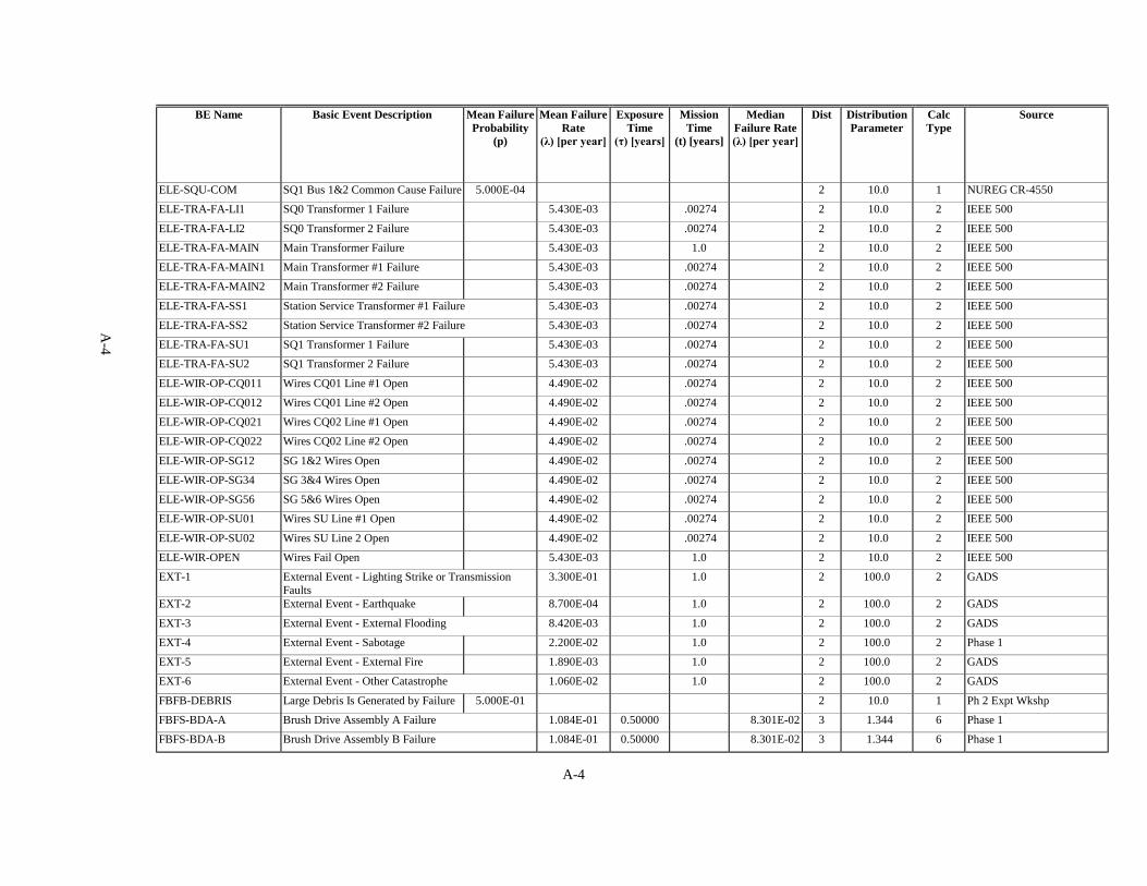
A-4

BE Name Basic Event Description Mean Failure Probability

(p)

Mean Failure Rate

(λ) [per year]

Exposure Time

(τ) [years]

Mission Time

(t) [years]

Median Failure Rate (λ) [per year]

Dist Distribution Parameter

Calc Type

Source

ELE-SQU-COM SQ1 Bus 1&2 Common Cause Failure 5.000E-04 2 10.0 1 NUREG CR-4550

ELE-TRA-FA-LI1 SQ0 Transformer 1 Failure 5.430E-03 .00274 2 10.0 2 IEEE 500

ELE-TRA-FA-LI2 SQ0 Transformer 2 Failure 5.430E-03 .00274 2 10.0 2 IEEE 500

ELE-TRA-FA-MAIN Main Transformer Failure 5.430E-03 1.0 2 10.0 2 IEEE 500

ELE-TRA-FA-MAIN1 Main Transformer #1 Failure 5.430E-03 .00274 2 10.0 2 IEEE 500

ELE-TRA-FA-MAIN2 Main Transformer #2 Failure 5.430E-03 .00274 2 10.0 2 IEEE 500

ELE-TRA-FA-SS1 Station Service Transformer #1 Failure 5.430E-03 .00274 2 10.0 2 IEEE 500

ELE-TRA-FA-SS2 Station Service Transformer #2 Failure 5.430E-03 .00274 2 10.0 2 IEEE 500

ELE-TRA-FA-SU1 SQ1 Transformer 1 Failure 5.430E-03 .00274 2 10.0 2 IEEE 500

ELE-TRA-FA-SU2 SQ1 Transformer 2 Failure 5.430E-03 .00274 2 10.0 2 IEEE 500

ELE-WIR-OP-CQ011 Wires CQ01 Line #1 Open 4.490E-02 .00274 2 10.0 2 IEEE 500

ELE-WIR-OP-CQ012 Wires CQ01 Line #2 Open 4.490E-02 .00274 2 10.0 2 IEEE 500

ELE-WIR-OP-CQ021 Wires CQ02 Line #1 Open 4.490E-02 .00274 2 10.0 2 IEEE 500

ELE-WIR-OP-CQ022 Wires CQ02 Line #2 Open 4.490E-02 .00274 2 10.0 2 IEEE 500

ELE-WIR-OP-SG12 SG 1&2 Wires Open 4.490E-02 .00274 2 10.0 2 IEEE 500

ELE-WIR-OP-SG34 SG 3&4 Wires Open 4.490E-02 .00274 2 10.0 2 IEEE 500

ELE-WIR-OP-SG56 SG 5&6 Wires Open 4.490E-02 .00274 2 10.0 2 IEEE 500

ELE-WIR-OP-SU01 Wires SU Line #1 Open 4.490E-02 .00274 2 10.0 2 IEEE 500

ELE-WIR-OP-SU02 Wires SU Line 2 Open 4.490E-02 .00274 2 10.0 2 IEEE 500

ELE-WIR-OPEN Wires Fail Open 5.430E-03 1.0 2 10.0 2 IEEE 500

EXT-1 External Event - Lighting Strike or Transmission Faults

3.300E-01 1.0 2 100.0 2 GADS

EXT-2 External Event - Earthquake 8.700E-04 1.0 2 100.0 2 GADS

EXT-3 External Event - External Flooding 8.420E-03 1.0 2 100.0 2 GADS

EXT-4 External Event - Sabotage 2.200E-02 1.0 2 100.0 2 Phase 1

EXT-5 External Event - External Fire 1.890E-03 1.0 2 100.0 2 GADS

EXT-6 External Event - Other Catastrophe 1.060E-02 1.0 2 100.0 2 GADS

FBFB-DEBRIS Large Debris Is Generated by Failure 5.000E-01 2 10.0 1 Ph 2 Expt Wkshp

FBFS-BDA-A Brush Drive Assembly A Failure 1.084E-01 0.50000 8.301E-02 3 1.344 6 Phase 1

FBFS-BDA-B Brush Drive Assembly B Failure 1.084E-01 0.50000 8.301E-02 3 1.344 6 Phase 1

A-4

A-5

BE Name Basic Event Description Mean Failure Probability

(p)

Mean Failure Rate

(λ) [per year]

Exposure Time

(τ) [years]

Mission Time

(t) [years]

Median Failure Rate (λ) [per year]

Dist Distribution Parameter

Calc Type

Source

FBFS-BDA-C Brush Drive Assembly C Failure 1.084E-01 0.50000 8.301E-02 3 1.344 6 Phase 1

FBFS-FAIL-FLOW Fixed Bar Fish Screen Fails Due to High Flow and Jams an Intake Gate Open

5.000E-01 2 10.0 1 Ph 2 Expt Wkshp

FBFS-FRAME-A Fish Screen Frame A Failure 1.724E-03 0.50000 1.269E-03 3 1.181 6 Phase 1

FBFS-FRAME-B Fish Screen Frame B Failure 1.724E-03 0.50000 1.269E-03 3 1.181 6 Phase 1

FBFS-FRAME-C Fish Screen Frame C Failure 1.724E-03 0.50000 1.269E-03 3 1.181 6 Phase 1

FBFS-HANDLE-A FBFS "A" Handling Errors Occur 8.650E-01 2 10.0 1 Ph 2 Expt Wkshp

FBFS-HANDLE-B FBFS "B" Handling Errors Occur 8.650E-01 2 10.0 1 Ph 2 Expt Wkshp

FBFS-HANDLE-C FBFS "C" Handling Errors Occur 8.650E-01 2 10.0 1 Ph 2 Expt Wkshp

FBFS-PP-A Fish Screen Perforated Plate A Failure 8.447E-03 0.50000 7.778E-03 3 4.148 6 Phase 1

FBFS-PP-B Fish Screen Perforated Plate B Failure 8.447E-03 0.50000 7.778E-03 3 4.148 6 Phase 1

FBFS-PP-C Fish Screen Perforated Plate C Failure 8.447E-03 0.50000 7.778E-03 3 4.148 6 Phase 1

FBFS-SWEEP-BAR-A Sweep Bar A Failure 1.084E-02 0.50000 8.301E-03 3 1.344 6 Phase 1

FBFS-SWEEP-BAR-B Sweep Bar B Failure 1.084E-02 0.50000 8.301E-03 3 1.344 6 Phase 1

FBFS-SWEEP-BAR-C Sweep Bar C Failure 1.084E-02 0.50000 8.301E-03 3 1.344 6 Phase 1

FBFS-VBF-A Vertical Barrier Frame A Failure 1.710E-03 0.50000 3.298E-03 3 1.0 6 Phase 1

FBFS-VBF-B Vertical Barrier Frame B Failure 1.710E-03 0.50000 3.298E-03 3 1.0 6 Phase 1

FBFS-VBF-C Vertical Barrier Frame C Failure 1.710E-03 0.50000 3.298E-03 3 1.0 6 Phase 1

FBFS-VBPP-A Vertical Barrier Perforated Plate A Failure 2.090E-03 0.50000 2.918E-03 3 1.0 6 Phase 1

FBFS-VBPP-B Vertical Barrier Perforated Plate B Failure 2.090E-03 0.50000 2.918E-03 3 1.0 6 Phase 1

FBFS-VBPP-C Vertical Barrier Perforated Plate C Failure 2.090E-03 0.50000 2.918E-03 3 1.0 6 Phase 1

GOV-ACCUM Accumulator Tank Fails 2.395E-03 .00274 2.306E-03 3 8.867 2 Phase 1

GOV-APV Actuator Pilot Valve Sticks Open 2.679E-03 .00274 2.580E-03 3 8.974 2 Phase 1

GOV-DRIFT-OPEN Wicket Gates Fail to Drift Shut 1.000E-03 2 10.0 1 Ph 2 Expt Wkshp

GOV-E-OS-LIMIT1 Electrical Over-speed Limit Device #1 Fails 1.000E-02 1.00000 2 10.0 6 Screen Value

GOV-E-OS-LIMIT2 Electrical Over-speed Limit Device #2 Fails 1.000E-02 1.00000 2 10.0 6 Screen Value

GOV-E-SSG Speed Signal Generator Fails Low 2.007E-03 .00274 1.928E-03 3 8.386 2 Phase 1

GOV-GDV Gate Distributing Valve Sticks Open 4.727E-04 1.00000 3.787E-04 3 1.601 6 Phase 1

GOV-HYD-CONN Hydraulic Connections Fail 3.552E-04 .00274 2.681E-04 3 1.279 2 Phase 1

GOV-LAG-PUMP-1 Lag Pump #1 Failure 1.165E-02 .00274 1.155E-02 3 39.293 2 Phase 1

A-5

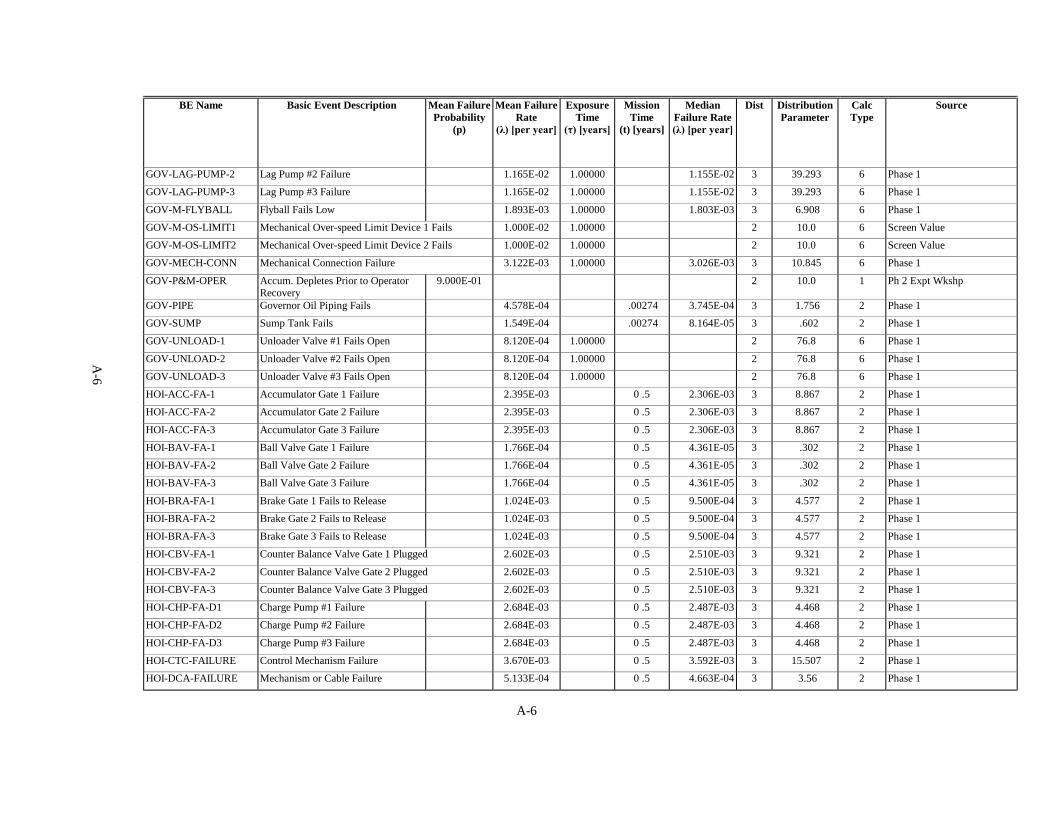
A-6

BE Name Basic Event Description Mean Failure Probability

(p)

Mean Failure Rate

(λ) [per year]

Exposure Time

(τ) [years]

Mission Time

(t) [years]

Median Failure Rate (λ) [per year]

Dist Distribution Parameter

Calc Type

Source

GOV-LAG-PUMP-2 Lag Pump #2 Failure 1.165E-02 1.00000 1.155E-02 3 39.293 6 Phase 1

GOV-LAG-PUMP-3 Lag Pump #3 Failure 1.165E-02 1.00000 1.155E-02 3 39.293 6 Phase 1

GOV-M-FLYBALL Flyball Fails Low 1.893E-03 1.00000 1.803E-03 3 6.908 6 Phase 1

GOV-M-OS-LIMIT1 Mechanical Over-speed Limit Device 1 Fails 1.000E-02 1.00000 2 10.0 6 Screen Value

GOV-M-OS-LIMIT2 Mechanical Over-speed Limit Device 2 Fails 1.000E-02 1.00000 2 10.0 6 Screen Value

GOV-MECH-CONN Mechanical Connection Failure 3.122E-03 1.00000 3.026E-03 3 10.845 6 Phase 1

GOV-P&M-OPER Accum. Depletes Prior to Operator Recovery

9.000E-01 2 10.0 1 Ph 2 Expt Wkshp

GOV-PIPE Governor Oil Piping Fails 4.578E-04 .00274 3.745E-04 3 1.756 2 Phase 1

GOV-SUMP Sump Tank Fails 1.549E-04 .00274 8.164E-05 3 .602 2 Phase 1

GOV-UNLOAD-1 Unloader Valve #1 Fails Open 8.120E-04 1.00000 2 76.8 6 Phase 1

GOV-UNLOAD-2 Unloader Valve #2 Fails Open 8.120E-04 1.00000 2 76.8 6 Phase 1

GOV-UNLOAD-3 Unloader Valve #3 Fails Open 8.120E-04 1.00000 2 76.8 6 Phase 1

HOI-ACC-FA-1 Accumulator Gate 1 Failure 2.395E-03 0 .5 2.306E-03 3 8.867 2 Phase 1

HOI-ACC-FA-2 Accumulator Gate 2 Failure 2.395E-03 0 .5 2.306E-03 3 8.867 2 Phase 1

HOI-ACC-FA-3 Accumulator Gate 3 Failure 2.395E-03 0 .5 2.306E-03 3 8.867 2 Phase 1

HOI-BAV-FA-1 Ball Valve Gate 1 Failure 1.766E-04 0 .5 4.361E-05 3 .302 2 Phase 1

HOI-BAV-FA-2 Ball Valve Gate 2 Failure 1.766E-04 0 .5 4.361E-05 3 .302 2 Phase 1

HOI-BAV-FA-3 Ball Valve Gate 3 Failure 1.766E-04 0 .5 4.361E-05 3 .302 2 Phase 1

HOI-BRA-FA-1 Brake Gate 1 Fails to Release 1.024E-03 0 .5 9.500E-04 3 4.577 2 Phase 1

HOI-BRA-FA-2 Brake Gate 2 Fails to Release 1.024E-03 0 .5 9.500E-04 3 4.577 2 Phase 1

HOI-BRA-FA-3 Brake Gate 3 Fails to Release 1.024E-03 0 .5 9.500E-04 3 4.577 2 Phase 1

HOI-CBV-FA-1 Counter Balance Valve Gate 1 Plugged 2.602E-03 0 .5 2.510E-03 3 9.321 2 Phase 1

HOI-CBV-FA-2 Counter Balance Valve Gate 2 Plugged 2.602E-03 0 .5 2.510E-03 3 9.321 2 Phase 1

HOI-CBV-FA-3 Counter Balance Valve Gate 3 Plugged 2.602E-03 0 .5 2.510E-03 3 9.321 2 Phase 1

HOI-CHP-FA-D1 Charge Pump #1 Failure 2.684E-03 0 .5 2.487E-03 3 4.468 2 Phase 1

HOI-CHP-FA-D2 Charge Pump #2 Failure 2.684E-03 0 .5 2.487E-03 3 4.468 2 Phase 1

HOI-CHP-FA-D3 Charge Pump #3 Failure 2.684E-03 0 .5 2.487E-03 3 4.468 2 Phase 1

HOI-CTC-FAILURE Control Mechanism Failure 3.670E-03 0 .5 3.592E-03 3 15.507 2 Phase 1

HOI-DCA-FAILURE Mechanism or Cable Failure 5.133E-04 0 .5 4.663E-04 3 3.56 2 Phase 1

A-6

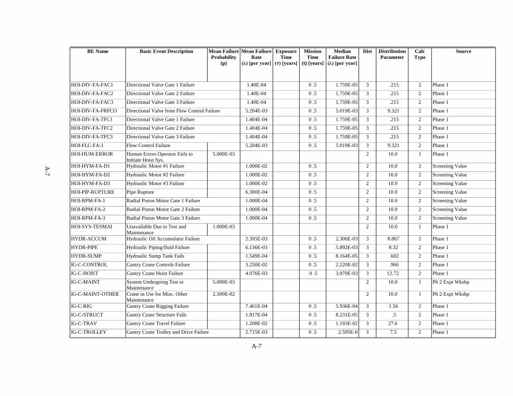
A-7

BE Name Basic Event Description Mean Failure Probability

(p)

Mean Failure Rate

(λ) [per year]

Exposure Time

(τ) [years]

Mission Time

(t) [years]

Median Failure Rate (λ) [per year]

Dist Distribution Parameter

Calc Type

Source

HOI-DIV-FA-FAC1 Directional Valve Gate 1 Failure 1.40E-04 0 .5 1.759E-05 3 .215 2 Phase 1

HOI-DIV-FA-FAC2 Directional Valve Gate 2 Failure 1.40E-04 0 .5 1.759E-05 3 .215 2 Phase 1

HOI-DIV-FA-FAC3 Directional Valve Gate 3 Failure 1.40E-04 0 .5 1.759E-05 3 .215 2 Phase 1

HOI-DIV-FA-FRFCO Directional Valve from Flow Control Failure 5.204E-03 0 .5 5.019E-03 3 9.321 2 Phase 1

HOI-DIV-FA-TFC1 Directional Valve Gate 1 Failure 1.404E-04 0 .5 1.759E-05 3 .215 2 Phase 1

HOI-DIV-FA-TFC2 Directional Valve Gate 2 Failure 1.404E-04 0 .5 1.759E-05 3 .215 2 Phase 1

HOI-DIV-FA-TFC3 Directional Valve Gate 3 Failure 1.404E-04 0 .5 1.759E-05 3 .215 2 Phase 1

HOI-FLC-FA-1 Flow Control Failure 5.204E-03 0 .5 5.019E-03 3 9.321 2 Phase 1

HOI-HUM-ERROR Human Errors Operator Fails to Initiate Hoist Sys.

5.000E-03 2 10.0 1 Phase 1

HOI-HYM-FA-D1 Hydraulic Motor #1 Failure 1.000E-02 0 .5 2 10.0 2 Screening Value

HOI-HYM-FA-D2 Hydraulic Motor #2 Failure 1.000E-02 0 .5 2 10.0 2 Screening Value

HOI-HYM-FA-D3 Hydraulic Motor #3 Failure 1.000E-02 0 .5 2 10.0 2 Screening Value

HOI-PIP-RUPTURE Pipe Rupture 6.300E-04 0 .5 2 10.0 2 Screening Value

HOI-RPM-FA-1 Radial Piston Motor Gate 1 Failure 1.000E-04 0 .5 2 10.0 2 Screening Value

HOI-RPM-FA-2 Radial Piston Motor Gate 2 Failure 1.000E-04 0 .5 2 10.0 2 Screening Value

HOI-RPM-FA-3 Radial Piston Motor Gate 3 Failure 1.000E-04 0 .5 2 10.0 2 Screening Value

HOI-SYS-TESMAI Unavailable Due to Test and Maintenance

1.000E-03 2 10.0 1 Phase 1

HYDR-ACCUM Hydraulic Oil Accumulator Failure 2.395E-03 0 .5 2.306E-03 3 8.867 2 Phase 1

HYDR-PIPE Hydraulic Piping/fluid Failure 6.136E-03 0 .5 5.892E-03 3 8.32 2 Phase 1

HYDR-SUMP Hydraulic Sump Tank Fails 1.549E-04 0 .5 8.164E-05 3 .602 2 Phase 1

IG-C-CONTROL Gantry Crane Controls Failure 3.250E-02 0 .5 2.220E-02 3 .966 2 Phase 1

IG-C-HOIST Gantry Crane Hoist Failure 4.076E-03 0 .5 3.970E-03 3 12.72 2 Phase 1

IG-C-MAINT System Undergoing Test or Maintenance

5.000E-03 2 10.0 1 Ph 2 Expt Wkshp

IG-C-MAINT-OTHER Crane in Use for Misc. Other Maintenance

2.500E-02 2 10.0 1 Ph 2 Expt Wkshp

IG-C-RIG Gantry Crane Rigging Failure 7.461E-04 0 .5 5.936E-04 3 1.56 2 Phase 1

IG-C-STRUCT Gantry Crane Structure Fails 1.817E-04 0 .5 8.231E-05 3 .5 2 Phase 1

IG-C-TRAV Gantry Crane Travel Failure 1.208E-02 0 .5 1.193E-02 3 27.6 2 Phase 1

IG-C-TROLLEY Gantry Crane Trolley and Drive Failure 2.715E-03 0 .5 2.595E-0 3 7.5 2 Phase 1

A-7

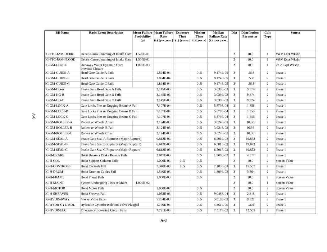
A-8

BE Name Basic Event Description Mean Failure Probability

(p)

Mean Failure Rate

(λ) [per year]

Exposure Time

(τ) [years]

Mission Time

(t) [years]

Median Failure Rate (λ) [per year]

Dist Distribution Parameter

Calc Type

Source

IG-FTC-JAM-DEBRI Debris Cause Jamming of Intake Gate 1.500E-01 2 10.0 1 V&V Expt Wkshp

IG-FTC-JAM-FLOOD Debris Cause Jamming of Intake Gate 1.500E-01 2 10.0 1 V&V Expt Wkshp

IG-GM-FORCE Runaway Water Dynamic Force Prevents Closure

1.000E-03 2 10.0 1 Ph 2 Expt Wkshp

IG-GM-GUIDE-A Head Gate Guide A Fails 1.894E-04 0 .5 9.174E-05 3 .538 2 Phase 1

IG-GM-GUIDE-B Head Gate Guide B Fails 1.894E-04 0 .5 9.174E-05 3 .538 2 Phase 1

IG-GM-GUIDE-C Head Gate Guide C Fails 1.894E-04 0 .5 9.174E-05 3 .538 2 Phase 1

IG-GM-HG-A Intake Gate Head Gate A Fails 3.145E-03 0 .5 3.039E-03 3 9.874 2 Phase 1

IG-GM-HG-B Intake Gate Head Gate B Fails 3.145E-03 0 .5 3.039E-03 3 9.874 2 Phase 1

IG-GM-HG-C Intake Gate Head Gate C Fails 3.145E-03 0 .5 3.039E-03 3 9.874 2 Phase 1

IG-GM-LOCK-A Gate Locks Pins or Dogging Beams A Fail 7.107E-04 0 .5 5.879E-04 3 1.856 2 Phase 1

IG-GM-LOCK-B Gate Locks Pins or Dogging Beams B Fail 7.107E-04 0 .5 5.879E-04 3 1.856 2 Phase 1

IG-GM-LOCK-C Gate Locks Pins or Dogging Beams C Fail 7.107E-04 0 .5 5.879E-04 3 1.856 2 Phase 1

IG-GM-ROLLER-A Rollers or Wheels A Fail 3.124E-03 0 .5 3.024E-03 3 10.36 2 Phase 1

IG-GM-ROLLER-B Rollers or Wheels B Fail 3.124E-03 0 .5 3.024E-03 3 10.36 2 Phase 1

IG-GM-ROLLER-C Rollers or Wheels C Fail 3.124E-03 0 .5 3.024E-03 3 10.36 2 Phase 1

IG-GM-SEAL-A Intake Gate Seal A Ruptures (Major Rupture) 6.612E-03 0 .5 6.501E-03 3 19.873 2 Phase 1

IG-GM-SEAL-B Intake Gate Seal B Ruptures (Major Rupture) 6.612E-03 0 .5 6.501E-03 3 19.873 2 Phase 1

IG-GM-SEAL-C Intake Gate Seal C Ruptures (Major Rupture) 6.612E-03 0 .5 6.501E-03 3 19.873 2 Phase 1

IG-H-BRAKE Hoist Brake or Brake Release Fails 2.047E-03 0 .5 1.900E-03 3 4.577 2 Phase 1

IG-H-COL Hoist Support Column Fails 1.000E-03 0 .5 0 .5 2 10.0 2 Screen Value

IG-H-CONTROLS Hoist Controls Fail 7.340E-03 0 .5 0 .5 7.183E-03 3 15.507 2 Phase 1

IG-H-DRUM Hoist Drum or Cables Fail 1.540E-03 0 .5 1.399E-03 3 3.564 2 Phase 1

IG-H-FRAME Hoist Frame Fails 1.000E-03 0 .5 2 10.0 2 Screen Value

IG-H-MAINT System Undergoing Tests or Maint 1.000E-02 2 10.0 1 Screen Value

IG-H-MOTOR Hoist Motor Fails 1.000E-02 0 .5 2 10.0 2 Screen Value

IG-H-SHEAVES Hoist Sheaves Fail 1.052E-03 0 .5 9.048E-04 3 2.318 2 Phase 1

IG-HYDR-4WAY 4-Way Valve Fails 5.204E-03 0 .5 5.019E-03 3 9.321 2 Phase 1

IG-HYDR-CYL-ISOL Hydraulic Cylinder Isolation Valve Plugged 1.766E-04 0 .5 4.361E-05 3 .302 2 Phase 1

IG-HYDR-ELC Emergency Lowering Circuit Fails 7.721E-03 0 .5 7.517E-03 3 12.505 2 Phase 1

A-8

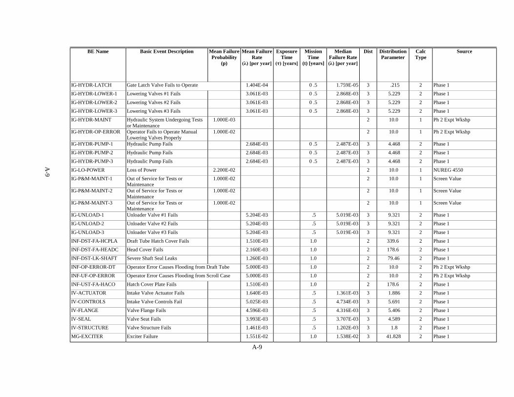
A-9

BE Name Basic Event Description Mean Failure Probability

(p)

Mean Failure Rate

(λ) [per year]

Exposure Time

(τ) [years]

Mission Time

(t) [years]

Median Failure Rate (λ) [per year]

Dist Distribution Parameter

Calc Type

Source

IG-HYDR-LATCH Gate Latch Valve Fails to Operate 1.404E-04 0 .5 1.759E-05 3 .215 2 Phase 1

IG-HYDR-LOWER-1 Lowering Valves #1 Fails 3.061E-03 0 .5 2.868E-03 3 5.229 2 Phase 1

IG-HYDR-LOWER-2 Lowering Valves #2 Fails 3.061E-03 0 .5 2.868E-03 3 5.229 2 Phase 1

IG-HYDR-LOWER-3 Lowering Valves #3 Fails 3.061E-03 0 .5 2.868E-03 3 5.229 2 Phase 1

IG-HYDR-MAINT Hydraulic System Undergoing Tests or Maintenance

1.000E-03 2 10.0 1 Ph 2 Expt Wkshp

IG-HYDR-OP-ERROR Operator Fails to Operate Manual Lowering Valves Properly

1.000E-02 2 10.0 1 Ph 2 Expt Wkshp

IG-HYDR-PUMP-1 Hydraulic Pump Fails 2.684E-03 0 .5 2.487E-03 3 4.468 2 Phase 1

IG-HYDR-PUMP-2 Hydraulic Pump Fails 2.684E-03 0 .5 2.487E-03 3 4.468 2 Phase 1

IG-HYDR-PUMP-3 Hydraulic Pump Fails 2.684E-03 0 .5 2.487E-03 3 4.468 2 Phase 1

IG-LO-POWER Loss of Power 2.200E-02 2 10.0 1 NUREG 4550

IG-P&M-MAINT-1 Out of Service for Tests or Maintenance

1.000E-02 2 10.0 1 Screen Value

IG-P&M-MAINT-2 Out of Service for Tests or Maintenance

1.000E-02 2 10.0 1 Screen Value

IG-P&M-MAINT-3 Out of Service for Tests or Maintenance

1.000E-02 2 10.0 1 Screen Value

IG-UNLOAD-1 Unloader Valve #1 Fails 5.204E-03 .5 5.019E-03 3 9.321 2 Phase 1

IG-UNLOAD-2 Unloader Valve #2 Fails 5.204E-03 .5 5.019E-03 3 9.321 2 Phase 1

IG-UNLOAD-3 Unloader Valve #3 Fails 5.204E-03 .5 5.019E-03 3 9.321 2 Phase 1

INF-DST-FA-HCPLA Draft Tube Hatch Cover Fails 1.510E-03 1.0 2 339.6 2 Phase 1

INF-DST-FA-HEADC Head Cover Fails 2.160E-03 1.0 2 178.6 2 Phase 1

INF-DST-LK-SHAFT Severe Shaft Seal Leaks 1.260E-03 1.0 2 79.46 2 Phase 1

INF-OP-ERROR-DT Operator Error Causes Flooding from Draft Tube 5.000E-03 1.0 2 10.0 2 Ph 2 Expt Wkshp

INF-UF-OP-ERROR Operator Error Causes Flooding from Scroll Case 5.000E-03 1.0 2 10.0 2 Ph 2 Expt Wkshp

INF-UST-FA-HACO Hatch Cover Plate Fails 1.510E-03 1.0 2 178.6 2 Phase 1

IV-ACTUATOR Intake Valve Actuator Fails 1.640E-03 .5 1.361E-03 3 1.886 2 Phase 1

IV-CONTROLS Intake Valve Controls Fail 5.025E-03 .5 4.734E-03 3 5.691 2 Phase 1

IV-FLANGE Valve Flange Fails 4.596E-03 .5 4.316E-03 3 5.406 2 Phase 1

IV-SEAL Valve Seat Fails 3.993E-03 .5 3.707E-03 3 4.589 2 Phase 1

IV-STRUCTURE Valve Structure Fails 1.461E-03 .5 1.202E-03 3 1.8 2 Phase 1

MG-EXCITER Exciter Failure 1.551E-02 1.0 1.538E-02 3 41.828 2 Phase 1

A-9

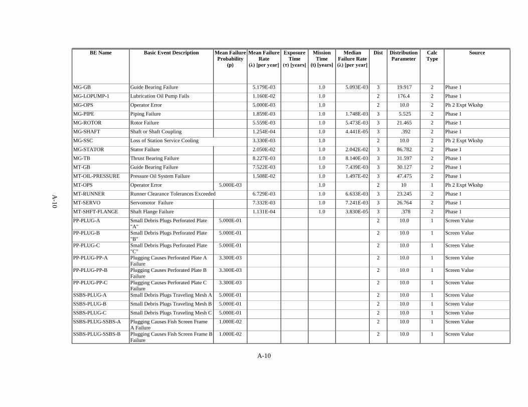
A-10

BE Name Basic Event Description Mean Failure Probability

(p)

Mean Failure Rate

(λ) [per year]

Exposure Time

(τ) [years]

Mission Time

(t) [years]

Median Failure Rate (λ) [per year]

Dist Distribution Parameter

Calc Type

Source

MG-GB Guide Bearing Failure 5.179E-03 1.0 5.093E-03 3 19.917 2 Phase 1

MG-LOPUMP-1 Lubrication Oil Pump Fails 1.160E-02 1.0 2 176.4 2 Phase 1

MG-OPS Operator Error 5.000E-03 1.0 2 10.0 2 Ph 2 Expt Wkshp

MG-PIPE Piping Failure 1.859E-03 1.0 1.748E-03 3 5.525 2 Phase 1

MG-ROTOR Rotor Failure 5.559E-03 1.0 5.473E-03 3 21.465 2 Phase 1

MG-SHAFT Shaft or Shaft Coupling 1.254E-04 1.0 4.441E-05 3 .392 2 Phase 1

MG-SSC Loss of Station Service Cooling 3.330E-03 1.0 2 10.0 2 Ph 2 Expt Wkshp

MG-STATOR Stator Failure 2.050E-02 1.0 2.042E-02 3 86.782 2 Phase 1

MG-TB Thrust Bearing Failure 8.227E-03 1.0 8.140E-03 3 31.597 2 Phase 1

MT-GB Guide Bearing Failure 7.522E-03 1.0 7.439E-03 3 30.127 2 Phase 1

MT-OIL-PRESSURE Pressure Oil System Failure 1.508E-02 1.0 1.497E-02 3 47.475 2 Phase 1

MT-OPS Operator Error 5.000E-03 1.0 2 10 1 Ph 2 Expt Wkshp

MT-RUNNER Runner Clearance Tolerances Exceeded 6.729E-03 1.0 6.633E-03 3 23.245 2 Phase 1

MT-SERVO Servomotor Failure 7.332E-03 1.0 7.241E-03 3 26.764 2 Phase 1

MT-SHFT-FLANGE Shaft Flange Failure 1.131E-04 1.0 3.830E-05 3 .378 2 Phase 1

PP-PLUG-A Small Debris Plugs Perforated Plate "A"

5.000E-01 2 10.0 1 Screen Value

PP-PLUG-B Small Debris Plugs Perforated Plate "B"

5.000E-01 2 10.0 1 Screen Value

PP-PLUG-C Small Debris Plugs Perforated Plate "C"

5.000E-01 2 10.0 1 Screen Value

PP-PLUG-PP-A Plugging Causes Perforated Plate A Failure

3.300E-03 2 10.0 1 Screen Value

PP-PLUG-PP-B Plugging Causes Perforated Plate B Failure

3.300E-03 2 10.0 1 Screen Value

PP-PLUG-PP-C Plugging Causes Perforated Plate C Failure

3.300E-03 2 10.0 1 Screen Value

SSBS-PLUG-A Small Debris Plugs Traveling Mesh A 5.000E-01 2 10.0 1 Screen Value

SSBS-PLUG-B Small Debris Plugs Traveling Mesh B 5.000E-01 2 10.0 1 Screen Value

SSBS-PLUG-C Small Debris Plugs Traveling Mesh C 5.000E-01 2 10.0 1 Screen Value

SSBS-PLUG-SSBS-A Plugging Causes Fish Screen Frame A Failure

1.000E-02 2 10.0 1 Screen Value

SSBS-PLUG-SSBS-B Plugging Causes Fish Screen Frame B Failure

1.000E-02 2 10.0 1 Screen Value

A-10

A-11

BE Name Basic Event Description Mean Failure Probability

(p)

Mean Failure Rate

(λ) [per year]

Exposure Time

(τ) [years]

Mission Time

(t) [years]

Median Failure Rate (λ) [per year]

Dist Distribution Parameter

Calc Type

Source

SSBS-PLUG-SSBS-C Plugging Causes Fish Screen Frame C Failure

1.000E-02 2 10.0 1 Screen Value

TE-A-GEN DROP GEN DROP 2.500E+00 1.0 2 10.0 2 Expert Workshop

TE-A-OP-ERROR Operator Error 3.000E-01 1.0 2 10.0 2 Ph 2 Expt Wkshp

TMFS-COND-JAM TMFS Jams Intake Gate Given It Has Failed

7.500E-01 2 10.0 1 V&V Expert Workshop

TMFS-DEBRIS Large Debris Is Generated by Fish Screen Failure

4.000E-01 2 10.0 1 Ph 2 Expt Wkshp

TMFS-FAIL-FLOW Traveling Mesh Fish Screen Fails Due to High Flow and Jams an Intake Gate Open

1.000E-01 2 10.0 1 Ph 2 Expt Wkshp

TMFS-FRAME-A Fish Screen Frame A Failure 1.724E-03 0.50000 1.269E-03 3 1.181 6 Phase 1

TMFS-FRAME-B Fish Screen Frame B Failure 1.724E-03 0.50000 1.269E-03 3 1.181 6 Phase 1

TMFS-FRAME-C Fish Screen Frame C Failure 1.724E-03 0.50000 1.269E-03 3 1.181 6 Phase 1

TMFS-HANDLE-A TMFS A Handling Error Occurs 8.650E-01 2 10.0 1 Ph 2 Expt Wkshp

TMFS-HANDLE-B TMFS B Handling Error Occurs 8.650E-01 2 10.0 1 Ph 2 Expt Wkshp

TMFS-HANDLE-C TMFS C Handling Error Occurs 8.650E-01 2 10.0 1 Ph 2 Expt Wkshp

TMFS-HANDLE-MAJ Error Results in Major Structural Damage

3.330E-03 2 10.0 1 Screen Value

TMFS-PP-A Fish Screen Perforated Plate A Failure 8.447E-03 0.50000 7.778E-03 3 4.148 6 Phase 1

TMFS-PP-B Fish Screen Perforated Plate B Failure 8.447E-03 0.50000 7.778E-03 3 4.148 6 Phase 1

TMFS-PP-C Fish Screen Perforated Plate C Failure 8.447E-03 0.50000 7.778E-03 3 4.148 6 Phase 1

TMFS-SDSA-A Screen Drive System Assembly A Failure 7.824E-03 0.50000 6.782E-03 3 2.434 6 Phase 1

TMFS-SDSA-B Screen Drive System Assembly B Failure 7.824E-03 0.50000 6.782E-03 3 2.434 6 Phase 1

TMFS-SDSA-C Screen Drive System Assembly C Failure 7.824E-03 0.50000 6.782E-03 3 2.434 6 Phase 1

TMFS-TM-A Traveling Mesh A Failure 3.089E-02 0.50000 2.892E-02 3 5.167 6 Phase 1

TMFS-TM-B Traveling Mesh B Failure 3.089E-02 0.50000 2.892E-02 3 5.167 6 Phase 1

TMFS-TM-C Traveling Mesh C Failure 3.089E-02 0.50000 2.892E-02 3 5.167 6 Phase 1

TMFS-VBF-A Vertical Barrier Frame A Failure 1.710E-03 0.50000 3.298E-03 3 1.0 6 Phase 1

TMFS-VBF-B Vertical Barrier Frame B Failure 1.710E-03 0.50000 3.298E-03 3 1.0 6 Phase 1

TMFS-VBF-C Vertical Barrier Frame C Failure 1.710E-03 0.50000 3.298E-03 3 1.0 6 Phase 1

TMFS-VBPP-A Vertical Barrier Perforated Plate A Failure 2.090E-03 0.50000 2.918E-03 3 1.0 6 Phase 1

TMFS-VBPP-B Vertical Barrier Perforated Plate B Failure 2.090E-03 0.50000 2.918E-03 3 1.0 6 Phase 1

A-11

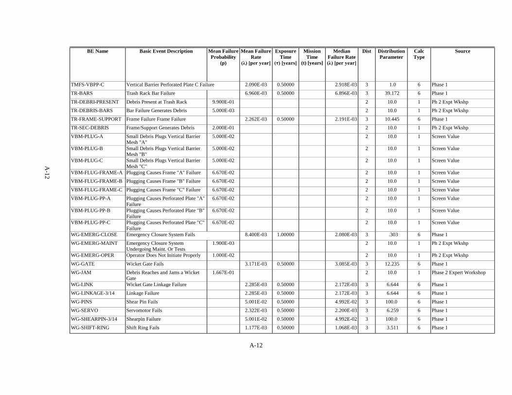
A-12

BE Name Basic Event Description Mean Failure Probability

(p)

Mean Failure Rate

(λ) [per year]

Exposure Time

(τ) [years]

Mission Time

(t) [years]

Median Failure Rate (λ) [per year]

Dist Distribution Parameter

Calc Type

Source

TMFS-VBPP-C Vertical Barrier Perforated Plate C Failure 2.090E-03 0.50000 2.918E-03 3 1.0 6 Phase 1

TR-BARS Trash Rack Bar Failure 6.960E-03 0.50000 6.896E-03 3 39.172 6 Phase 1

TR-DEBRI-PRESENT Debris Present at Trash Rack 9.900E-01 2 10.0 1 Ph 2 Expt Wkshp

TR-DEBRIS-BARS Bar Failure Generates Debris 5.000E-03 2 10.0 1 Ph 2 Expt Wkshp

TR-FRAME-SUPPORT Frame Failure Frame Failure 2.262E-03 0.50000 2.191E-03 3 10.445 6 Phase 1

TR-SEC-DEBRIS Frame/Support Generates Debris 2.000E-01 2 10.0 1 Ph 2 Expt Wkshp

VBM-PLUG-A Small Debris Plugs Vertical Barrier Mesh "A"

5.000E-02 2 10.0 1 Screen Value

VBM-PLUG-B Small Debris Plugs Vertical Barrier Mesh "B"

5.000E-02 2 10.0 1 Screen Value

VBM-PLUG-C Small Debris Plugs Vertical Barrier Mesh "C"

5.000E-02 2 10.0 1 Screen Value

VBM-FLUG-FRAME-A Plugging Causes Frame "A" Failure 6.670E-02 2 10.0 1 Screen Value

VBM-FLUG-FRAME-B Plugging Causes Frame "B" Failure 6.670E-02 2 10.0 1 Screen Value

VBM-FLUG-FRAME-C Plugging Causes Frame "C" Failure 6.670E-02 2 10.0 1 Screen Value

VBM-PLUG-PP-A Plugging Causes Perforated Plate "A" Failure

6.670E-02 2 10.0 1 Screen Value

VBM-PLUG-PP-B Plugging Causes Perforated Plate "B" Failure

6.670E-02 2 10.0 1 Screen Value

VBM-PLUG-PP-C Plugging Causes Perforated Plate "C" Failure

6.670E-02 2 10.0 1 Screen Value

WG-EMERG-CLOSE Emergency Closure System Fails 8.400E-03 1.00000 2.080E-03 3 .303 6 Phase 1

WG-EMERG-MAINT Emergency Closure System Undergoing Maint. Or Tests

1.900E-03 2 10.0 1 Ph 2 Expt Wkshp

WG-EMERG-OPER Operator Does Not Initiate Properly 1.000E-02 2 10.0 1 Ph 2 Expt Wkshp

WG-GATE Wicket Gate Fails 3.171E-03 0.50000 3.085E-03 3 12.235 6 Phase 1

WG-JAM Debris Reaches and Jams a Wicket Gate

1.667E-01 2 10.0 1 Phase 2 Expert Workshop

WG-LINK Wicket Gate Linkage Failure 2.285E-03 0.50000 2.172E-03 3 6.644 6 Phase 1

WG-LINKAGE-3/14 Linkage Failure 2.285E-03 0.50000 2.172E-03 3 6.644 6 Phase 1

WG-PINS Shear Pin Fails 5.001E-02 0.50000 4.992E-02 3 100.0 6 Phase 1

WG-SERVO Servomotor Fails 2.322E-03 0.50000 2.200E-03 3 6.259 6 Phase 1

WG-SHEARPIN-3/14 Shearpin Failure 5.001E-02 0.50000 4.992E-02 3 100.0 6 Phase 1

WG-SHIFT-RING Shift Ring Fails 1.177E-03 0.50000 1.068E-03 3 3.511 6 Phase 1

A-12

Appendix B

Initiating Event Trees

B-1

Appendix B. Initiating Event Trees This appendix presents the fault trees used to determine the frequency of powerhouse events that could require rapid closure of the intake gates. These trees were developed from the logic models of the various systems and structures involved in the operation and control of the powerhouse. Two types of events were considered, loss-of-load initiating events and flooding events. Loss-of-load events are those in which the electrical load of the grid is abruptly disconnected from the generator. Without this load the turbine/generator combination would over-speed unless either the wicket gates closed to control water flow through the turbine, or, failing that, the intake gates were closed. The fault tree used for the initial evaluation of the frequency of loss-of-load initiating events is presented in Figure B.1. Figures B.2 through B.6 present continuations of the tree in Figure B.1, expanding each of the subevents identified with triangular symbols in Figure B.1. Two types of flooding initiating events were considered. Upstream flooding events refer to powerhouse flooding from a source upstream of the wicket gates, in particular through the scroll case door. Upstream flooding events can be terminated only by closure of the intake gates, as the flooding source is upstream of the wicket gates. The fault tree used for the initial evaluation of the frequency of upstream flooding initiating events is presented in Figure B.7. Downstream flooding events refer to flooding from sources downstream of the wicket gates. These include sources such as the draft tube access hatch and the turbine head cover and shaft packing. Either wicket gate closure or intake gate closure can terminate downstream flooding events. The fault tree used for the initial evaluation of the frequency of downstream flooding initiating events is presented in Figure B.8.

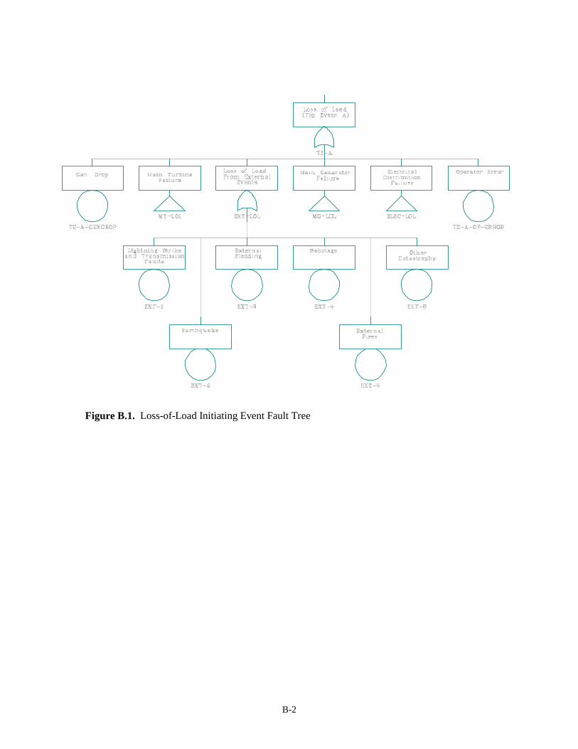
B-2

Figure B.1. Loss-of-Load Initiating Event Fault Tree

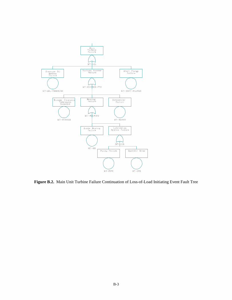
B-3

Figure B.2. Main Unit Turbine Failure Continuation of Loss-of-Load Initiating Event Fault Tree

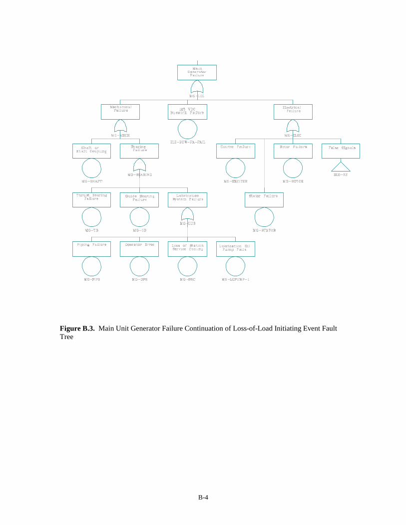
B-4

Figure B.3. Main Unit Generator Failure Continuation of Loss-of-Load Initiating Event Fault Tree

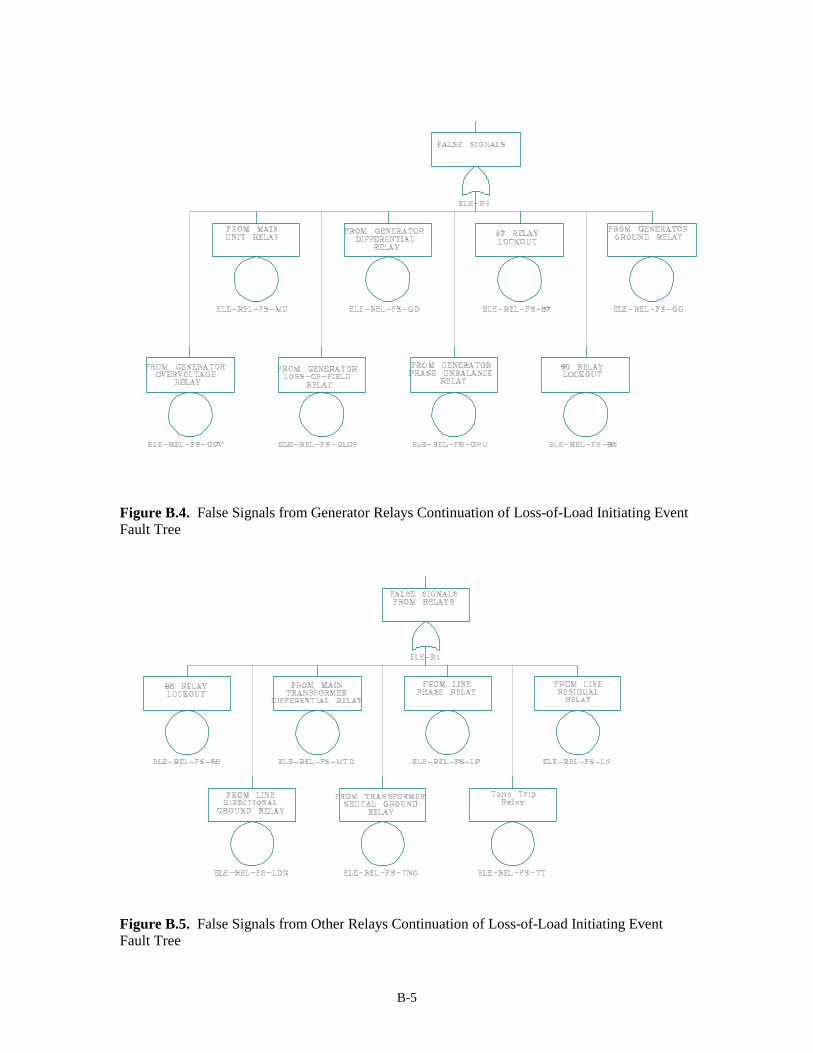
B-5

Figure B.4. False Signals from Generator Relays Continuation of Loss-of-Load Initiating Event Fault Tree

Figure B.5. False Signals from Other Relays Continuation of Loss-of-Load Initiating Event Fault Tree

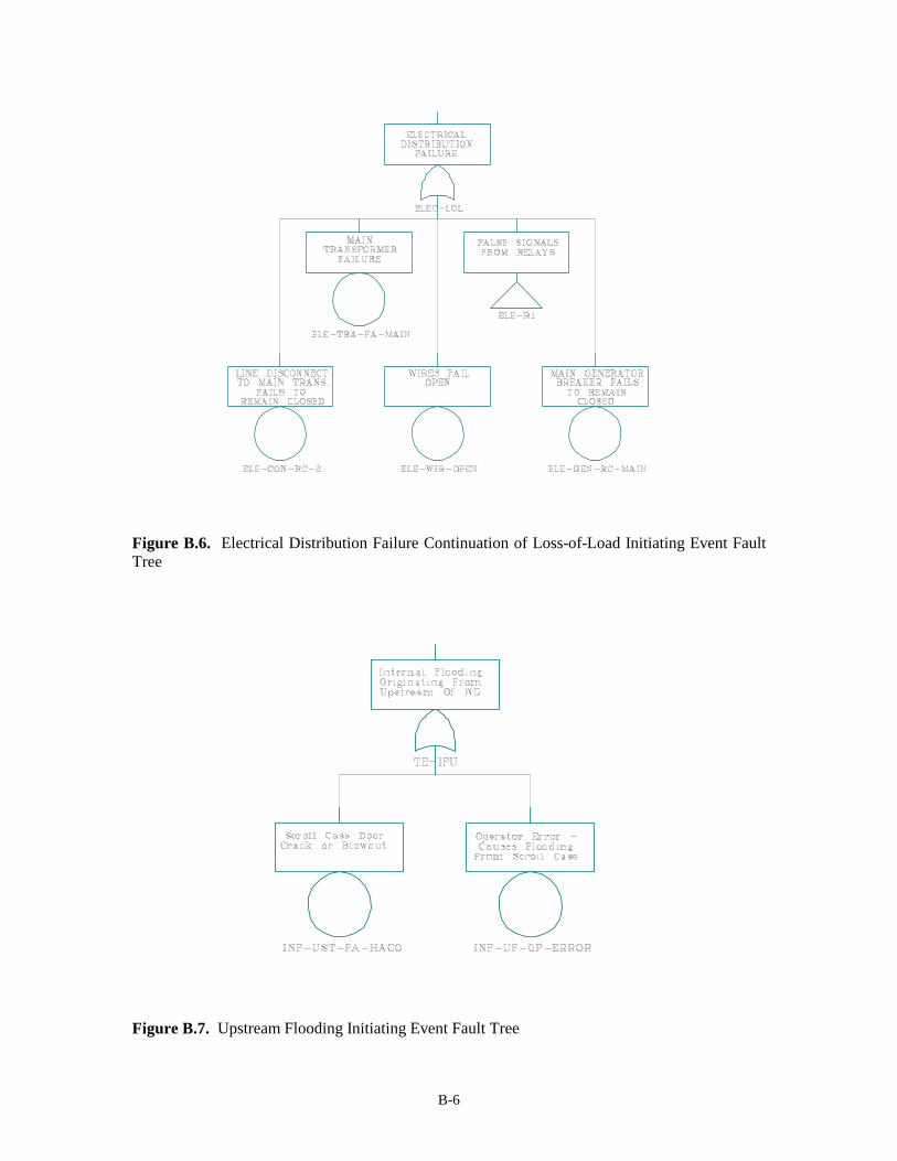
B-6

Figure B.6. Electrical Distribution Failure Continuation of Loss-of-Load Initiating Event Fault Tree

Figure B.7. Upstream Flooding Initiating Event Fault Tree

B-7

Figure B.8. Downstream Flooding Initiating Event Fault Tree

Appendix C

System Failure Fault Trees

C-1

Appendix C. System Failure Fault Trees This appendix presents the fault trees used to determine the probability of system failures, given that an initiating event has happened, that would lead to failure to control the initiating event. These trees were developed from the logic models of the various systems and structures involved in the operation and control of the powerhouse. The fault trees are used to determine the event combinations that can lead to failure of the wicket gates to close and terminate loss-of-load events or downstream flooding events, and the event combinations that can lead to failure of the intake gates to close and terminate loss-of-load events, upstream flooding events, and downstream flooding events. It should be noted that different fault trees are used for different initiating events. This situation is because different problems need different responses. For instance, on a loss-of-load event the wicket gate governor system must sense and respond to the need to control turbine over-speed, and then the mechanical part of the wicket gate system must operate successfully to close the wicket gates. This progression is addressed in Figure C.1, and continued in Figure C.2 through Figure C.9. The failure of the intake gates to close on a loss-of-load initiating event is addressed in Figure C.10, and continued in Figure C.11 through Figure C.31. On a downstream flooding event, the system must simply respond properly to operator commands to close the wicket gate; the governor is not involved. This is addressed in Figure C.32. It should be noted that two transfer gates on this figure refer to previous figures. Thus, IG-DEBRI refers to Figure C.22 and its continuation, and TE-C-RUN refers to Figure C.1 and its continuation. The failure of intake gates to close on either an upstream or downstream flooding initiating event is addressed in Figure C.33. Several transfer gates on this figure refer to previous figures. Finally, electrical power is required for the operation of most of the systems. Electrical power failures are addressed in Figure C.34 through Figure C.49, that relate to transfers into various types of the system failure fault trees.

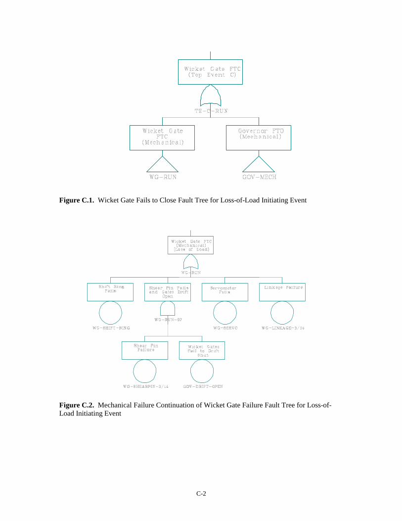
C-2

Figure C.1. Wicket Gate Fails to Close Fault Tree for Loss-of-Load Initiating Event

Figure C.2. Mechanical Failure Continuation of Wicket Gate Failure Fault Tree for Loss-of-Load Initiating Event

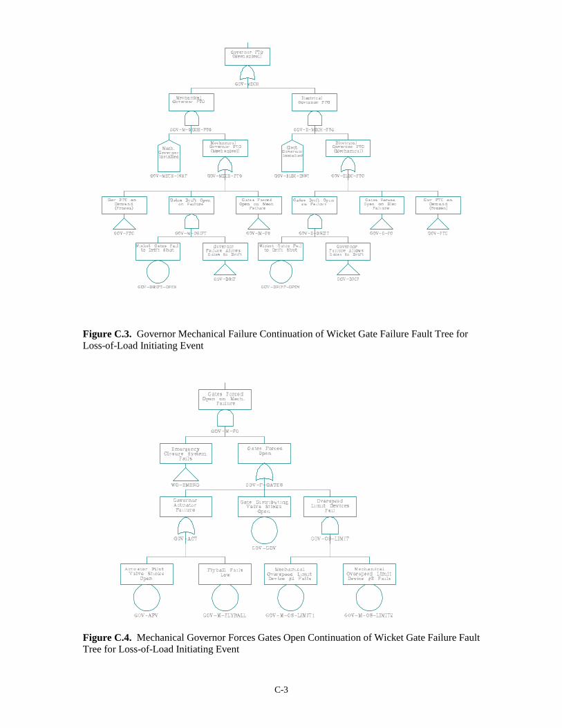
C-3

Figure C.3. Governor Mechanical Failure Continuation of Wicket Gate Failure Fault Tree for Loss-of-Load Initiating Event

Figure C.4. Mechanical Governor Forces Gates Open Continuation of Wicket Gate Failure Fault Tree for Loss-of-Load Initiating Event

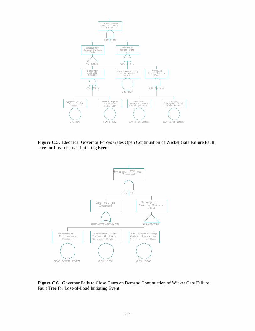
C-4

Figure C.5. Electrical Governor Forces Gates Open Continuation of Wicket Gate Failure Fault Tree for Loss-of-Load Initiating Event

Figure C.6. Governor Fails to Close Gates on Demand Continuation of Wicket Gate Failure Fault Tree for Loss-of-Load Initiating Event

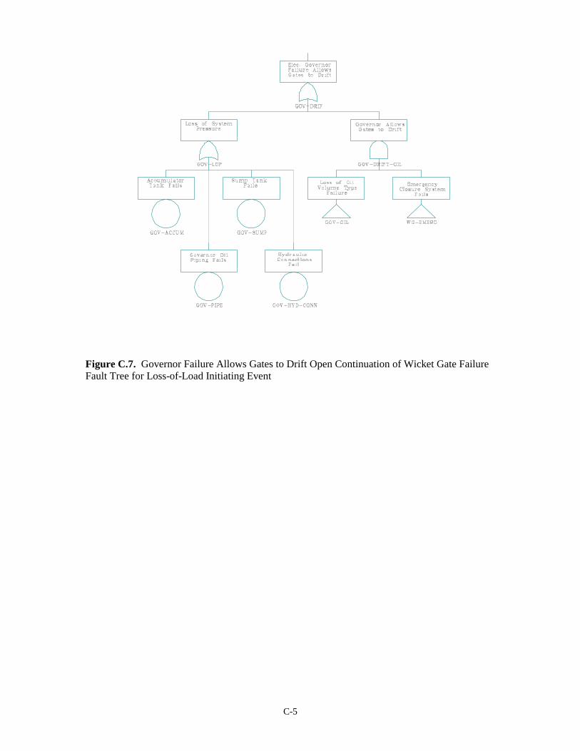
C-5

Figure C.7. Governor Failure Allows Gates to Drift Open Continuation of Wicket Gate Failure Fault Tree for Loss-of-Load Initiating Event

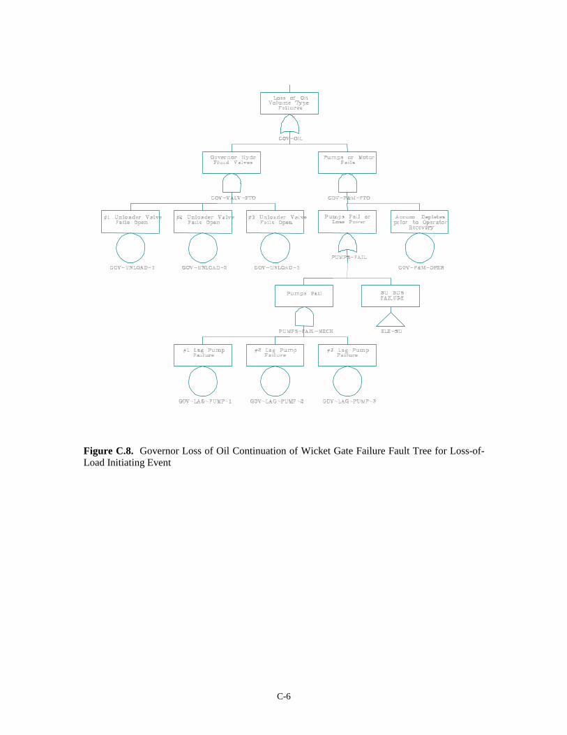
C-6

Figure C.8. Governor Loss of Oil Continuation of Wicket Gate Failure Fault Tree for Loss-of-Load Initiating Event

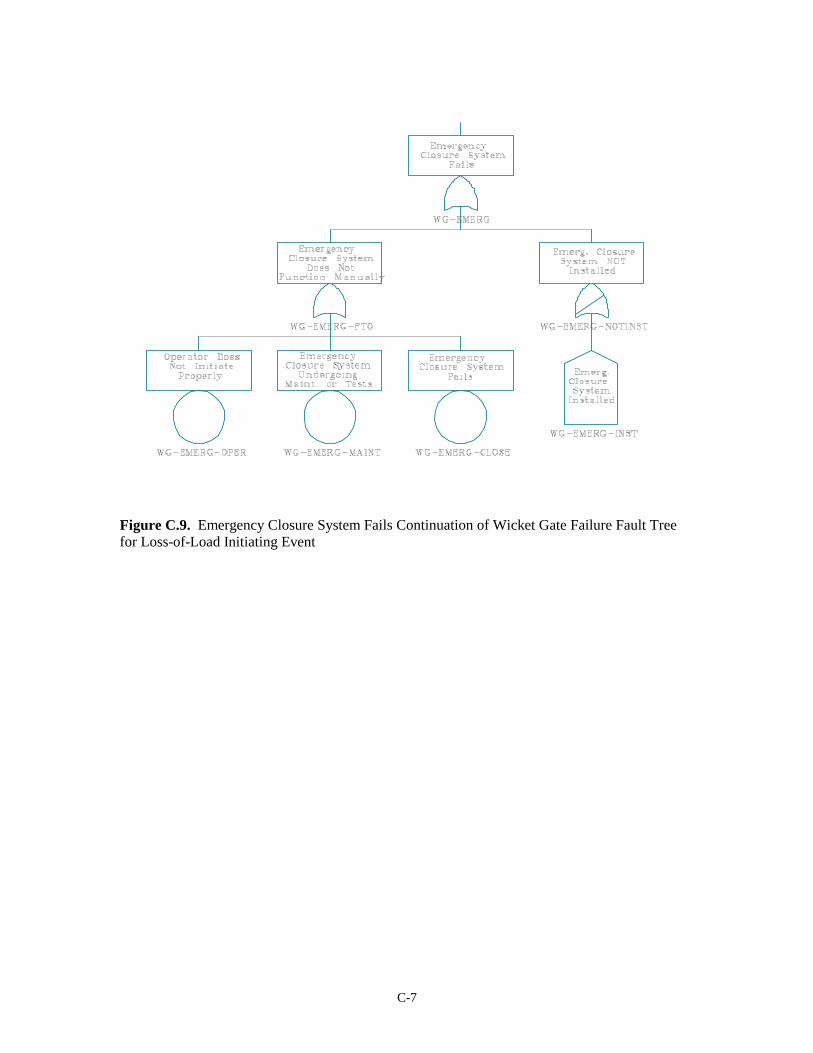
C-7

Figure C.9. Emergency Closure System Fails Continuation of Wicket Gate Failure Fault Tree for Loss-of-Load Initiating Event

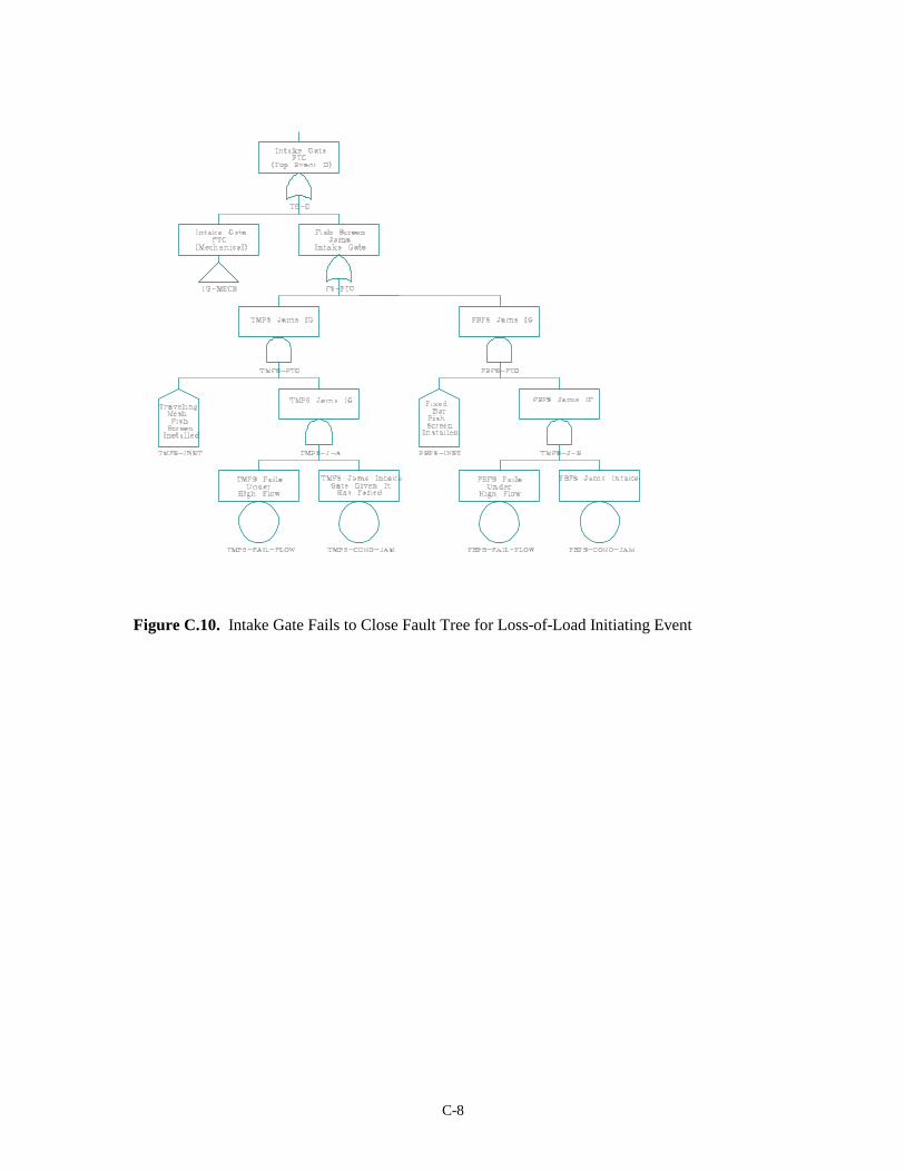
C-8

Figure C.10. Intake Gate Fails to Close Fault Tree for Loss-of-Load Initiating Event

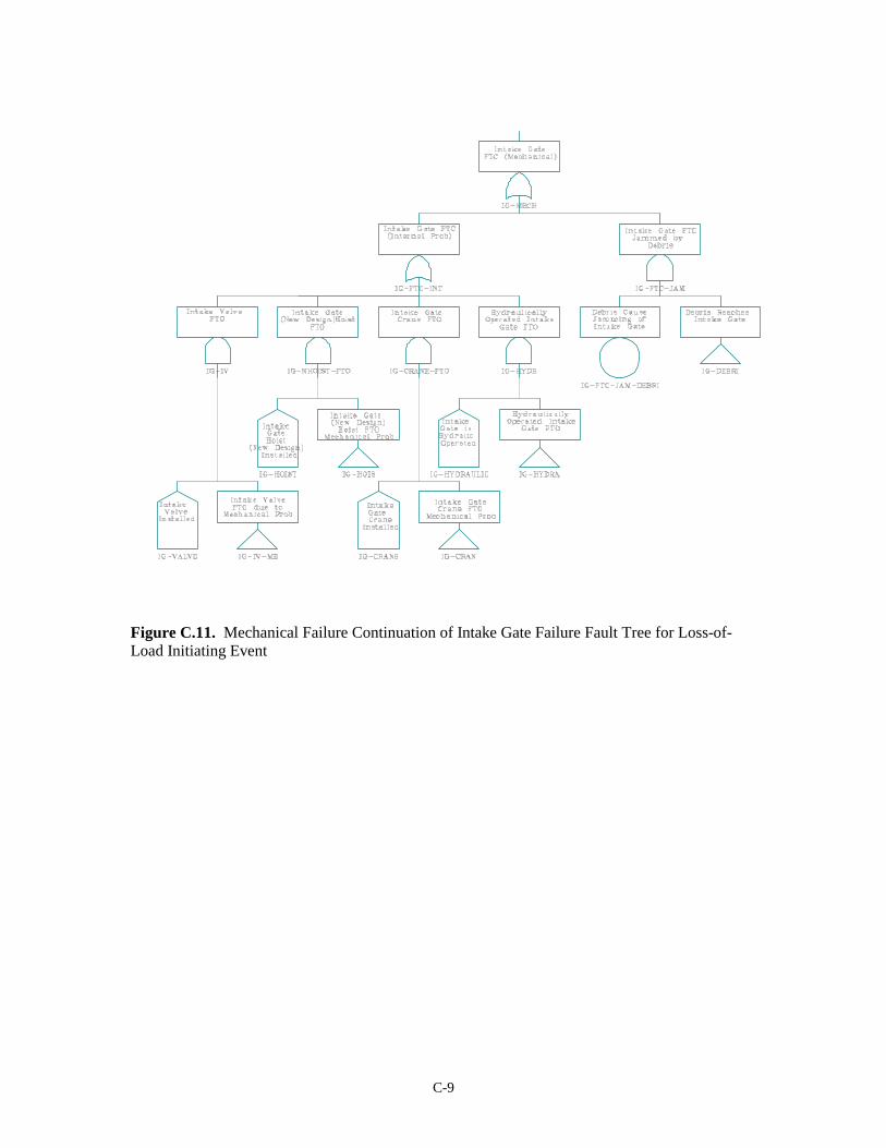
C-9

Figure C.11. Mechanical Failure Continuation of Intake Gate Failure Fault Tree for Loss-of-Load Initiating Event

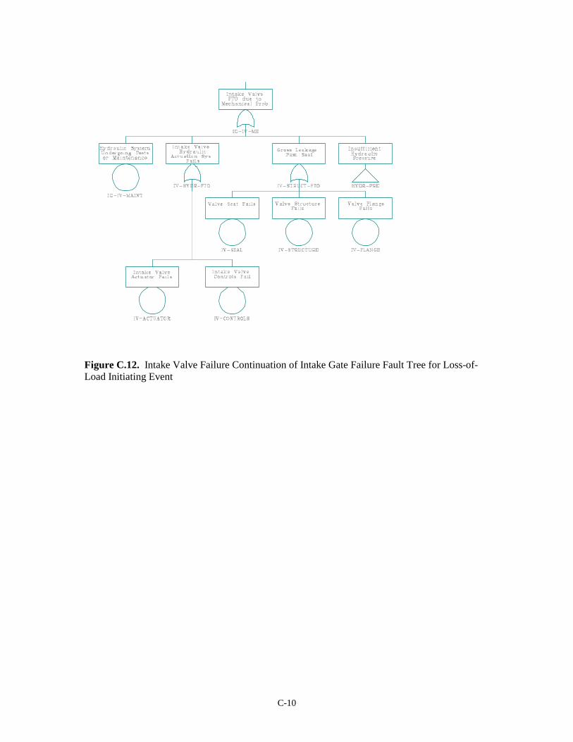
C-10

Figure C.12. Intake Valve Failure Continuation of Intake Gate Failure Fault Tree for Loss-of-Load Initiating Event

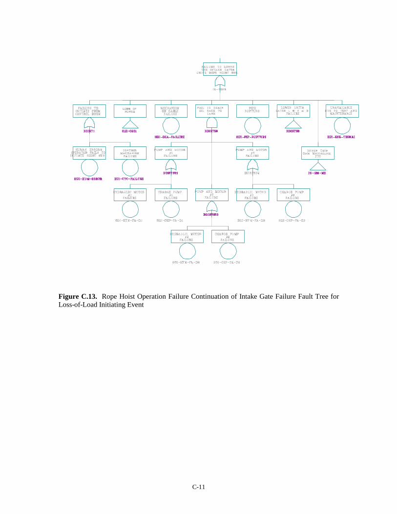
C-11

Figure C.13. Rope Hoist Operation Failure Continuation of Intake Gate Failure Fault Tree for Loss-of-Load Initiating Event

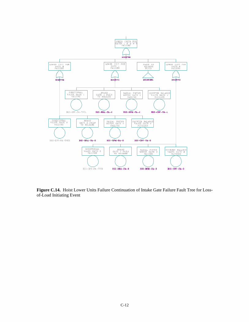
C-12

Figure C.14. Hoist Lower Units Failure Continuation of Intake Gate Failure Fault Tree for Loss-of-Load Initiating Event

C-13

Figure C.15. Hoist Fails to Release Fluid Continuation of Intake Gate Failure Fault Tree for Loss-of-Load Initiating Event

Figure C.16. Crane Operation Failure Continuation of Intake Gate Failure Fault Tree for Loss-of-Load Initiating Event

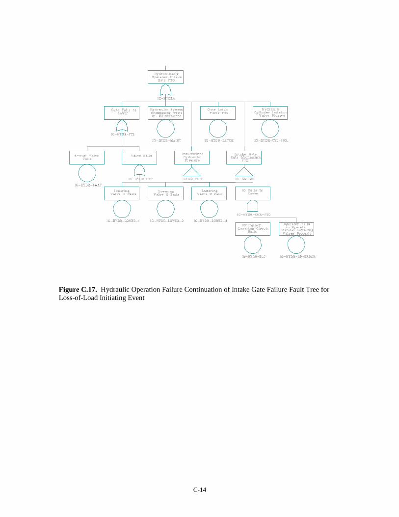
C-14

Figure C.17. Hydraulic Operation Failure Continuation of Intake Gate Failure Fault Tree for Loss-of-Load Initiating Event

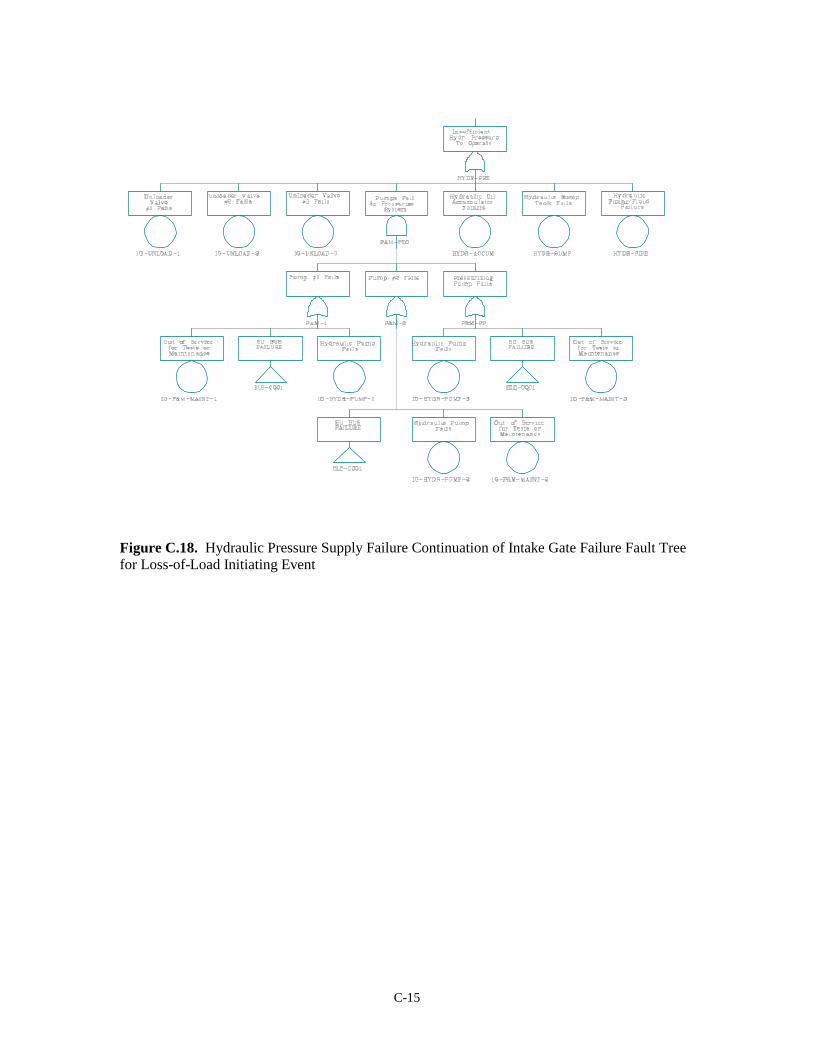
C-15

Figure C.18. Hydraulic Pressure Supply Failure Continuation of Intake Gate Failure Fault Tree for Loss-of-Load Initiating Event

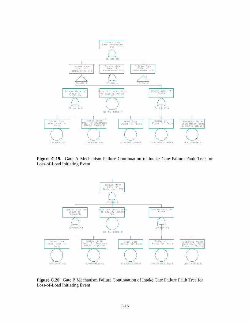
C-16

Figure C.19. Gate A Mechanism Failure Continuation of Intake Gate Failure Fault Tree for Loss-of-Load Initiating Event

Figure C.20. Gate B Mechanism Failure Continuation of Intake Gate Failure Fault Tree for Loss-of-Load Initiating Event

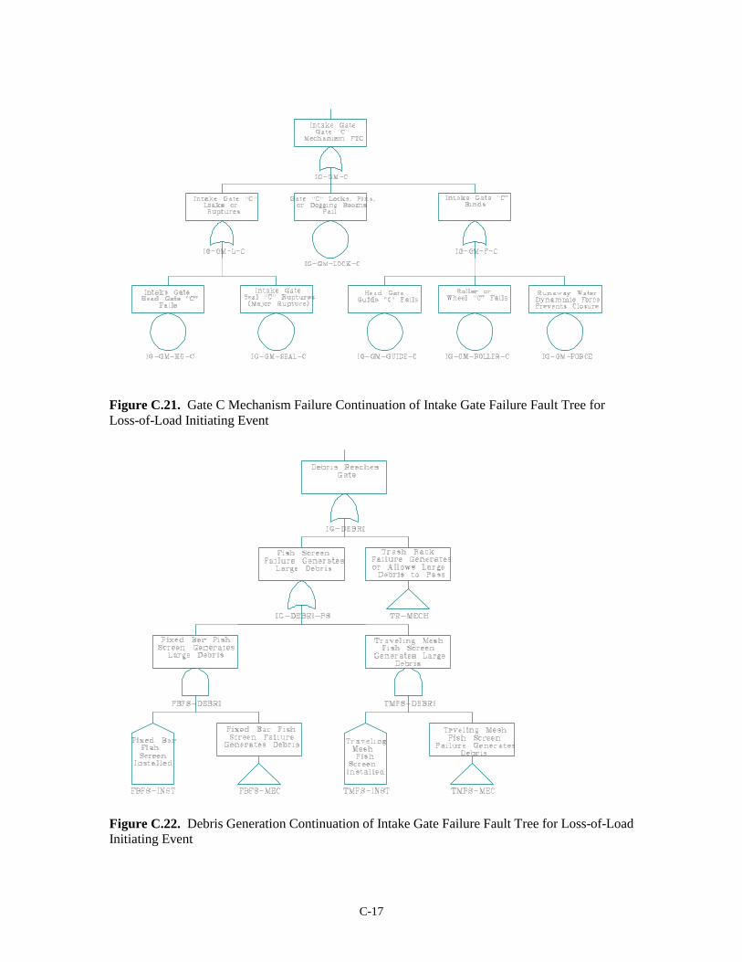
C-17

Figure C.21. Gate C Mechanism Failure Continuation of Intake Gate Failure Fault Tree for Loss-of-Load Initiating Event

Figure C.22. Debris Generation Continuation of Intake Gate Failure Fault Tree for Loss-of-Load Initiating Event

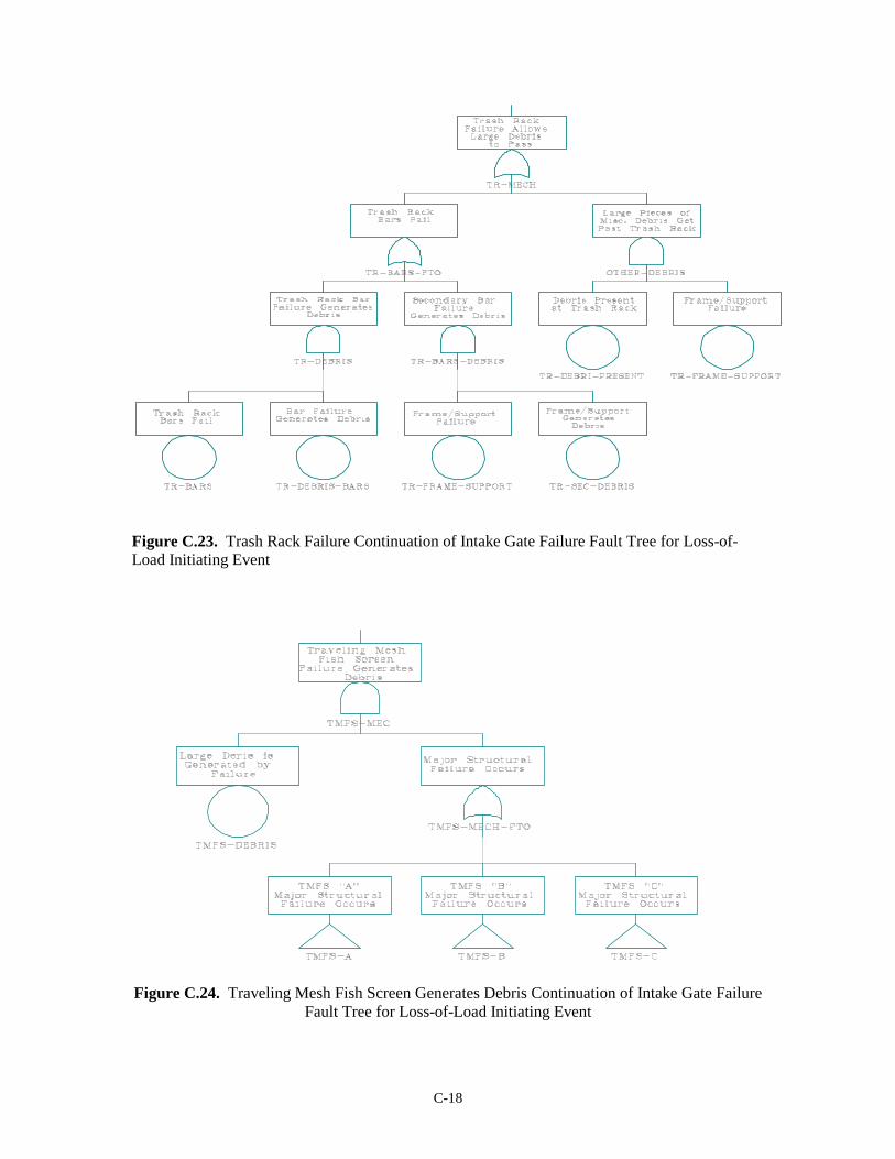
C-18

Figure C.23. Trash Rack Failure Continuation of Intake Gate Failure Fault Tree for Loss-of-Load Initiating Event

Figure C.24. Traveling Mesh Fish Screen Generates Debris Continuation of Intake Gate Failure Fault Tree for Loss-of-Load Initiating Event

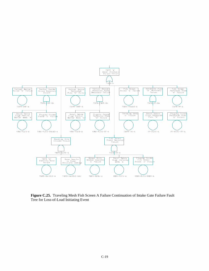
C-19

Figure C.25. Traveling Mesh Fish Screen A Failure Continuation of Intake Gate Failure Fault Tree for Loss-of-Load Initiating Event

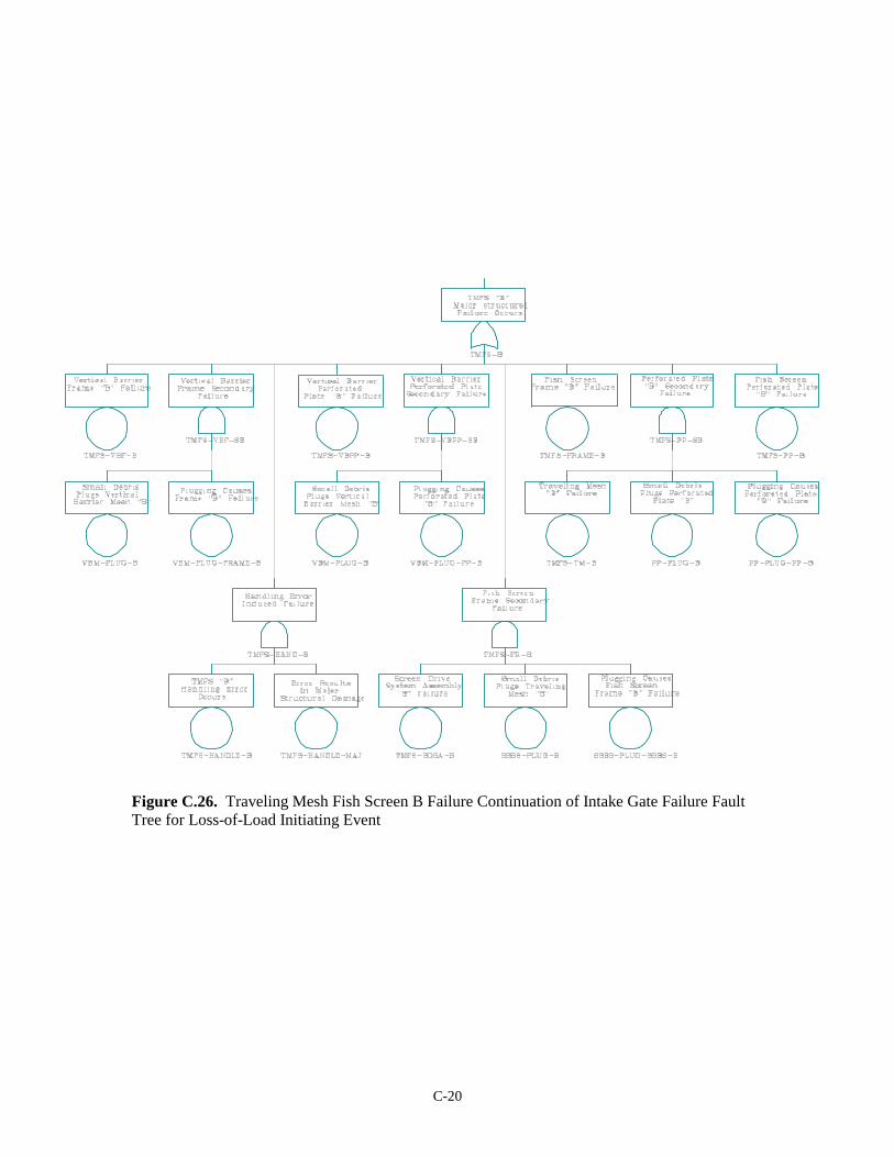
C-20

Figure C.26. Traveling Mesh Fish Screen B Failure Continuation of Intake Gate Failure Fault Tree for Loss-of-Load Initiating Event

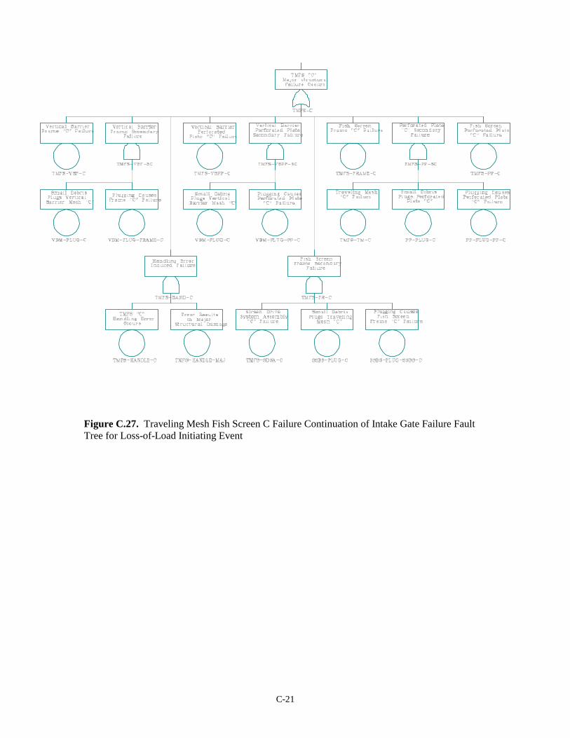
C-21

Figure C.27. Traveling Mesh Fish Screen C Failure Continuation of Intake Gate Failure Fault Tree for Loss-of-Load Initiating Event

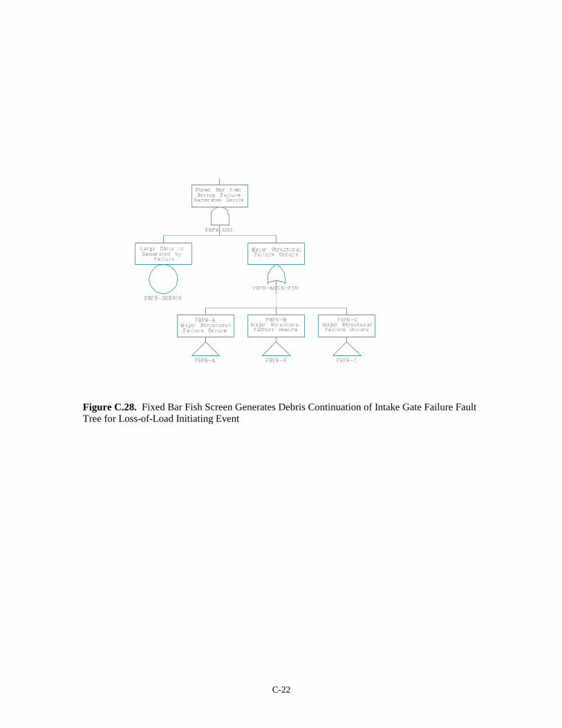
C-22

Figure C.28. Fixed Bar Fish Screen Generates Debris Continuation of Intake Gate Failure Fault Tree for Loss-of-Load Initiating Event

C-23

Figure C.29. Fixed Bar Fish Screen A Failure Continuation of Intake Gate Failure Fault Tree for Loss-of-Load Initiating Event

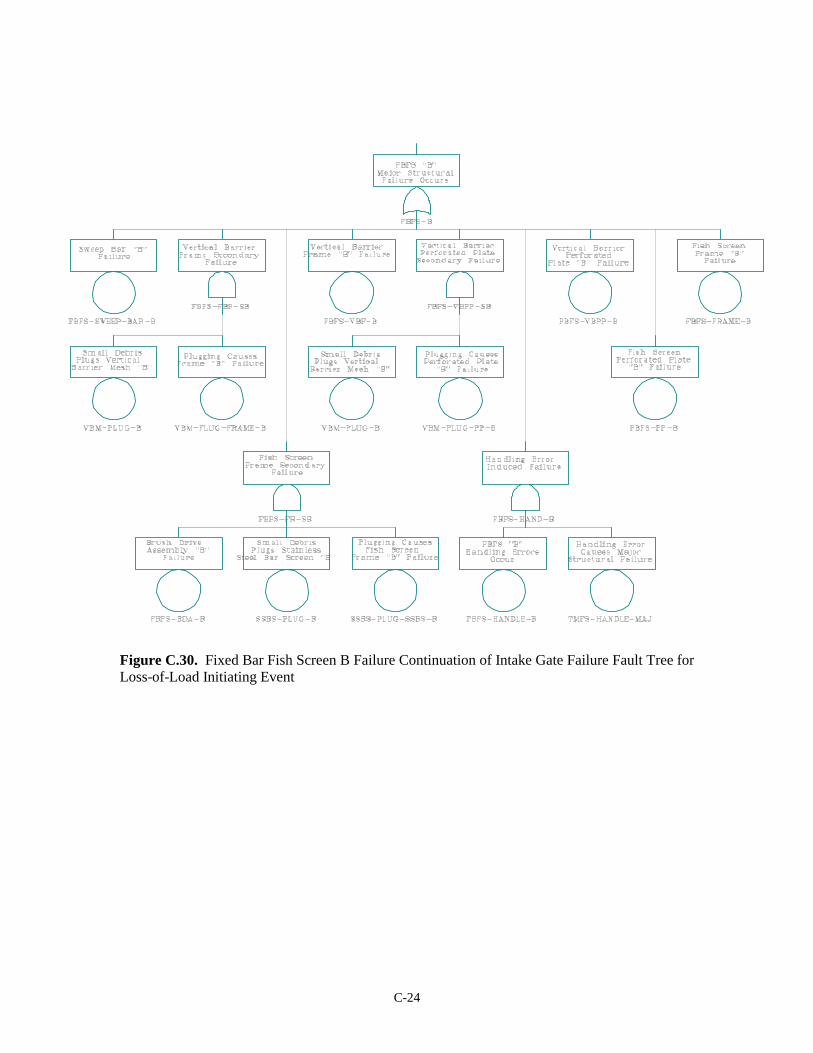
C-24

Figure C.30. Fixed Bar Fish Screen B Failure Continuation of Intake Gate Failure Fault Tree for Loss-of-Load Initiating Event

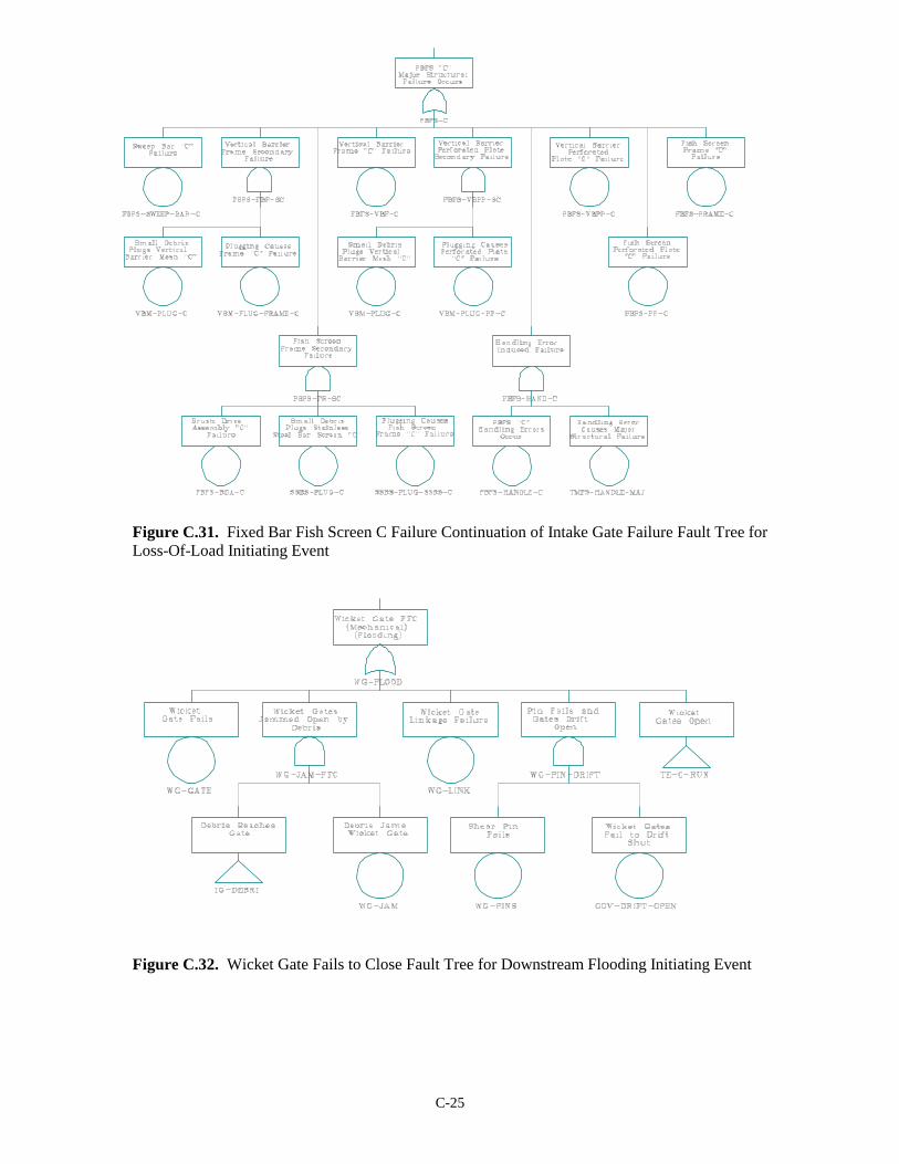
C-25

Figure C.31. Fixed Bar Fish Screen C Failure Continuation of Intake Gate Failure Fault Tree for Loss-Of-Load Initiating Event

Figure C.32. Wicket Gate Fails to Close Fault Tree for Downstream Flooding Initiating Event

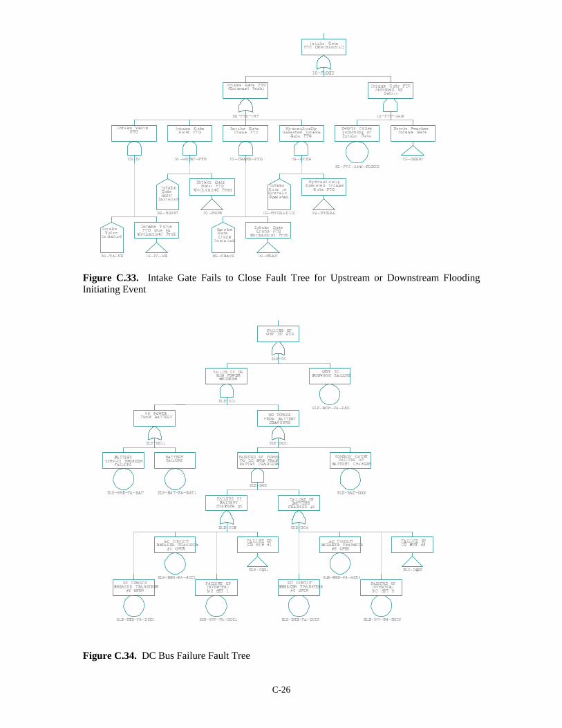
C-26

Figure C.33. Intake Gate Fails to Close Fault Tree for Upstream or Downstream Flooding Initiating Event

Figure C.34. DC Bus Failure Fault Tree

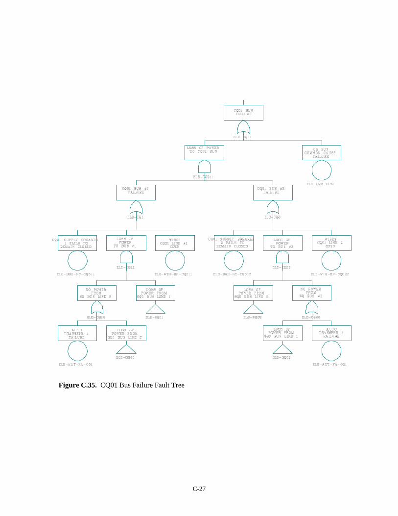
C-27

Figure C.35. CQ01 Bus Failure Fault Tree

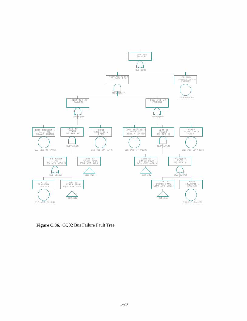
C-28

Figure C.36. CQ02 Bus Failure Fault Tree

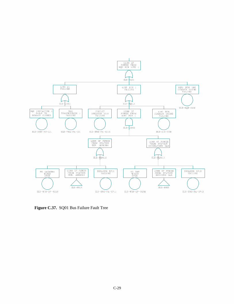
C-29

Figure C.37. SQ01 Bus Failure Fault Tree

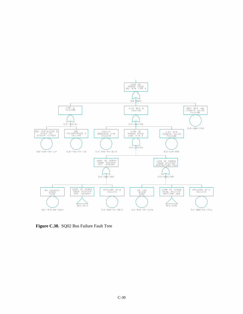
C-30

Figure C.38. SQ02 Bus Failure Fault Tree

C-31

Figure C.39. SQ1 Bus Failure Fault Tree

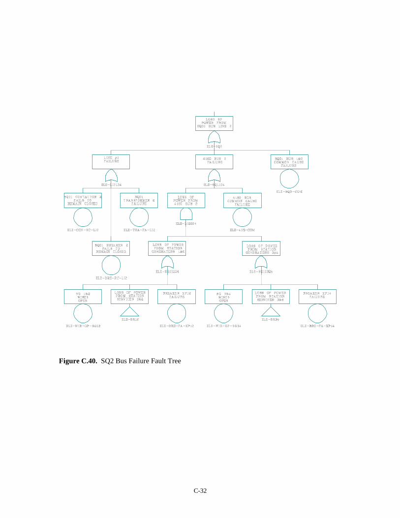
C-32

Figure C.40. SQ2 Bus Failure Fault Tree

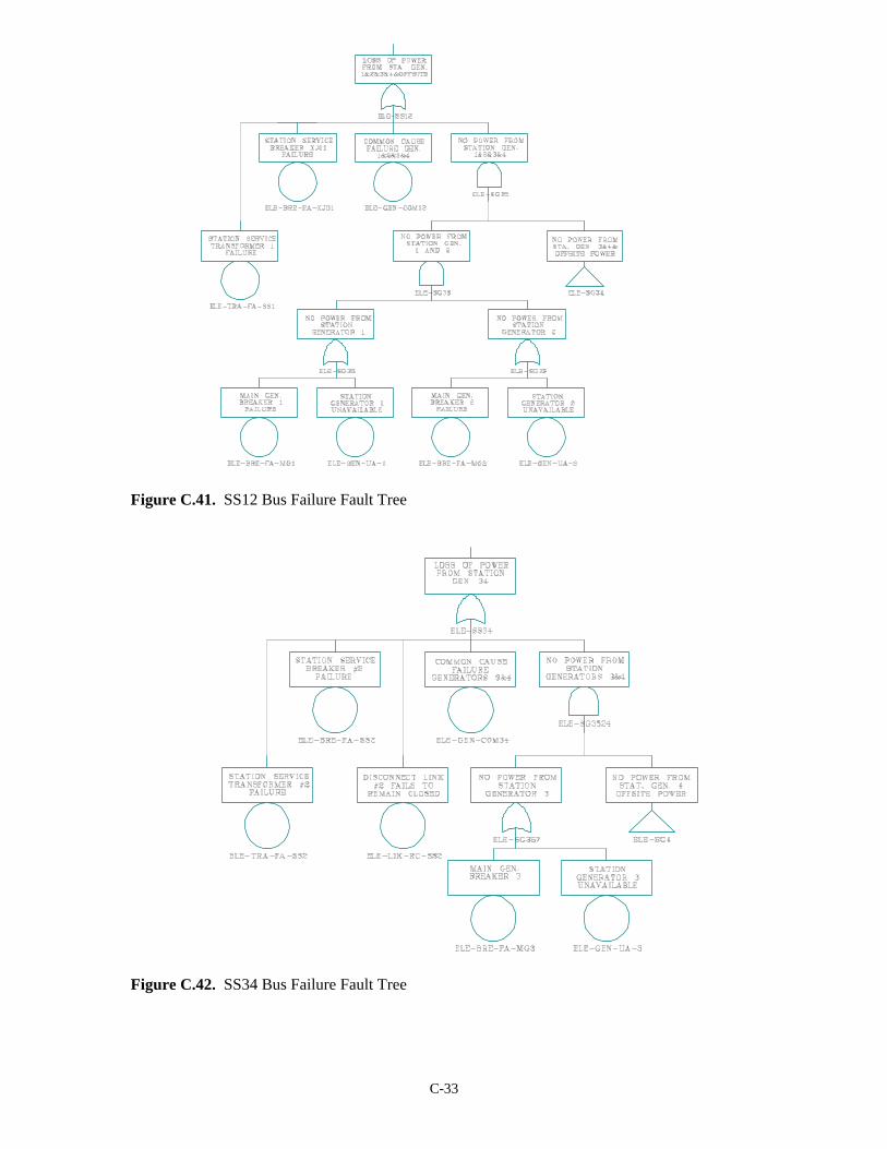
C-33

Figure C.41. SS12 Bus Failure Fault Tree

Figure C.42. SS34 Bus Failure Fault Tree

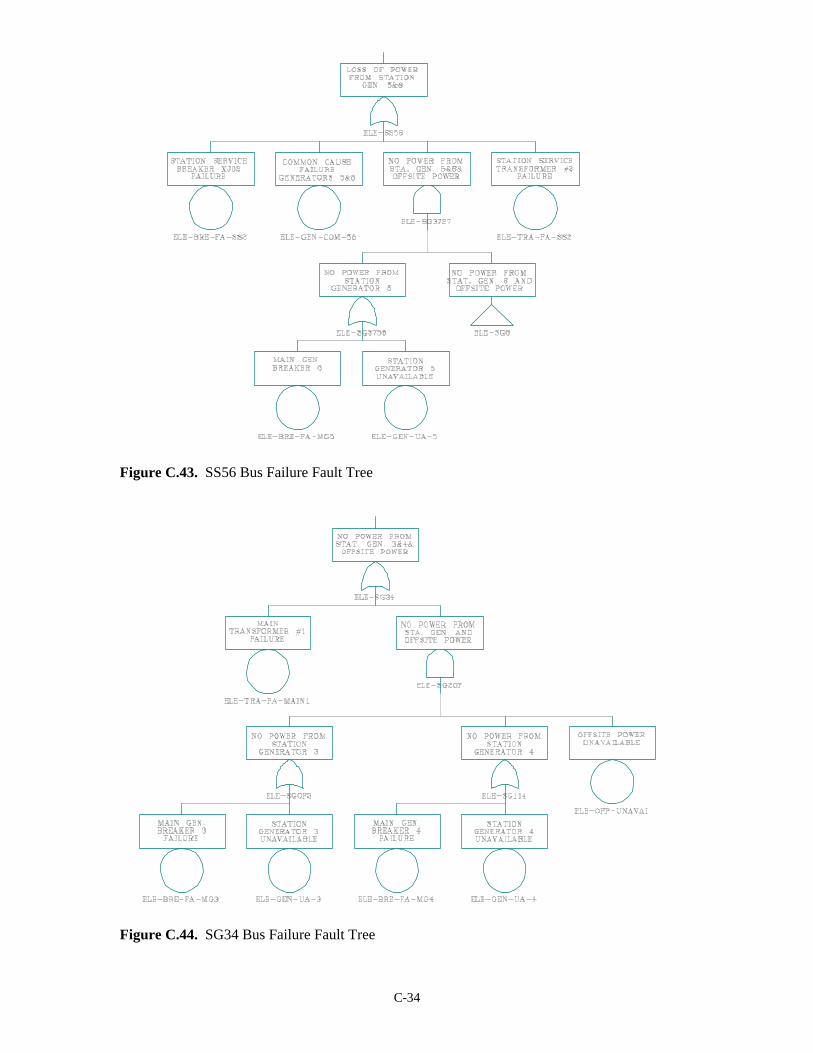
C-34

Figure C.43. SS56 Bus Failure Fault Tree

Figure C.44. SG34 Bus Failure Fault Tree

C-35

Figure C.45. SG4 Bus Failure Fault Tree

Figure C.46. SG6 Bus Failure Fault Tree

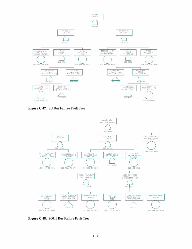
C-36

Figure C.47. SU Bus Failure Fault Tree

Figure C.48. SQU1 Bus Failure Fault Tree

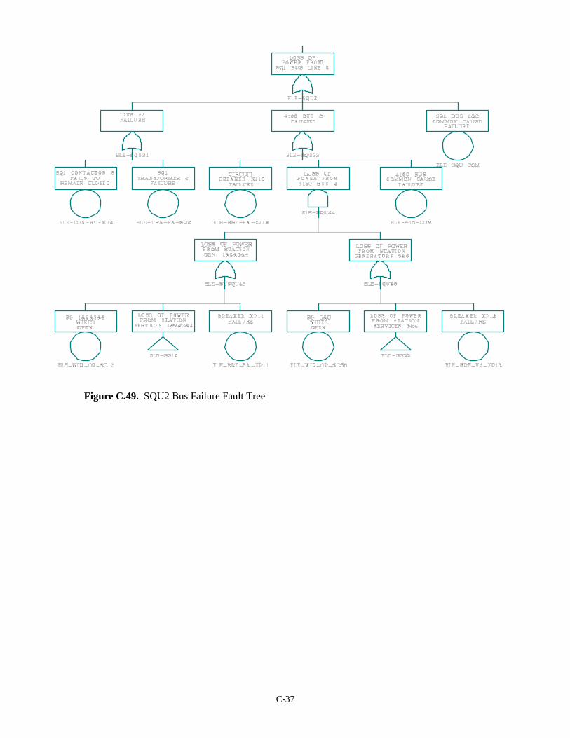
C-37

Figure C.49. SQU2 Bus Failure Fault Tree

Appendix D

Damage State Cost Estimate Inputs

D-1

Appendix D. Damage State Cost Estimate Inputs This appendix presents additional information supporting the calculations described in the body of the document in Section 2.3.2 Damage State Cost Development. D.1 Construction Costs COE cost engineers developed estimates of the costs to repair the damages associated with each of the over-speed states and the flooding states. An initial step in the cost estimation process was to describe the work required for each necessary activity. Cost estimates for the over-speed-with-flooding states were developed by adding the costs for the appropriate over-speed and flooding states, taking care to exclude double counting of activities that were duplicated in the two work descriptions. These combined costs are presented in the Construction columns of Table 2.26 and Table 2.27. Figures D.1 to D.9 present the cost summary sheets identifying the required work activities and associated repair costs for the five over-speed damage states and for the four flooding states that result in damages. D.2 Lost Power Costs

Equation 2.11 in Section 2.3.2.2 was used to calculate the costs of lost power generation from RPCu, the per-unit incremental energy replacement cost, FEu, the per-unit incremental foregone energy, and tu, the per-unit time-out-of-service. These costs are evaluated individually for each unit out of service. The COE provided inputs to RPCu and FEu from previous detailed studies for Lower Granite (LWG) (small-plant with 6 units) and John Day (JDA) (large plant with 16 units). Specifically for LWG, the analysis is based on sequential stream flow regulation model (HYSSR) study BIOP3/BIOP94, for JDA, the analysis is based on HYSSR study RF9596F. The COE ran HYSSR to obtain a period-by-period estimate of project generation with all units available. HYSSR uses a monthly time interval (except for April and August, that are split into two periods each) and a 60-year period of record (August 1928 through July 1988). Because other Power Branch models (including PCSAM) currently able to manage only 50 years of data, HYSSR output used in most power impact studies is limited to the August 1928 through July 1978 time period. The COE modified the HYSSR output to obtain a period-by-period estimate of project generation with one or more units unavailable. In simple generator rewind studies (like LWG) where rehabilitation of turbines is not under consideration, estimates are obtained using a spreadsheet analysis. In major rehabilitation studies (like JDA) where rehabilitation of turbines is under consideration, estimates are obtained using the HALLO model, that is able to model turbine characteristics in considerable detail. Because the time and effort required to develop turbine characteristics is so great, the HALLO model approach is used only in major rehabilitation studies. The COE used the period-of-record estimates of project generation with all units available and with one or more units unavailable as input to the system analysis model (PCSAM). PCSAM is

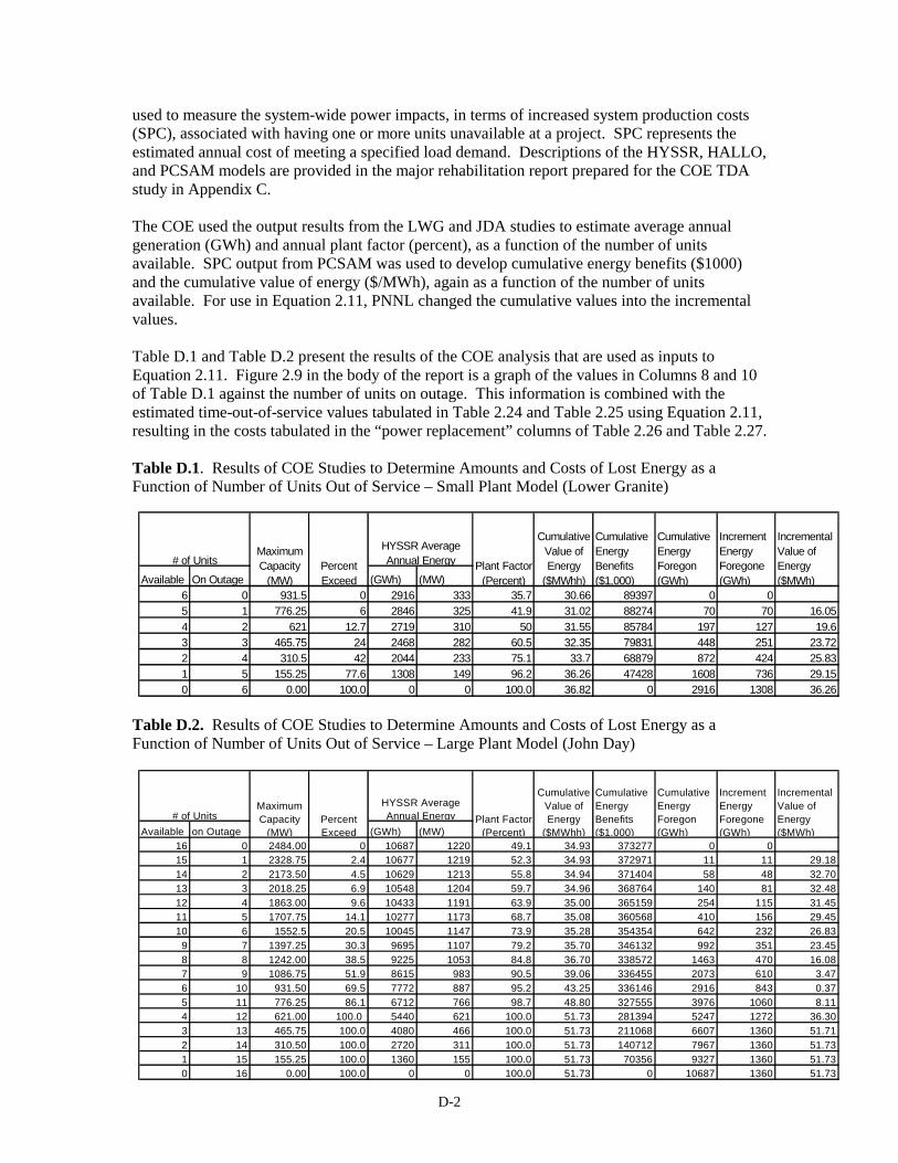
D-2

used to measure the system-wide power impacts, in terms of increased system production costs (SPC), associated with having one or more units unavailable at a project. SPC represents the estimated annual cost of meeting a specified load demand. Descriptions of the HYSSR, HALLO, and PCSAM models are provided in the major rehabilitation report prepared for the COE TDA study in Appendix C. The COE used the output results from the LWG and JDA studies to estimate average annual generation (GWh) and annual plant factor (percent), as a function of the number of units available. SPC output from PCSAM was used to develop cumulative energy benefits ($1000) and the cumulative value of energy ($/MWh), again as a function of the number of units available. For use in Equation 2.11, PNNL changed the cumulative values into the incremental values. Table D.1 and Table D.2 present the results of the COE analysis that are used as inputs to Equation 2.11. Figure 2.9 in the body of the report is a graph of the values in Columns 8 and 10 of Table D.1 against the number of units on outage. This information is combined with the estimated time-out-of-service values tabulated in Table 2.24 and Table 2.25 using Equation 2.11, resulting in the costs tabulated in the “power replacement” columns of Table 2.26 and Table 2.27. Table D.1. Results of COE Studies to Determine Amounts and Costs of Lost Energy as a Function of Number of Units Out of Service – Small Plant Model (Lower Granite)

Table D.2. Results of COE Studies to Determine Amounts and Costs of Lost Energy as a Function of Number of Units Out of Service – Large Plant Model (John Day)

Available On Outage (GWh) (MW)6 0 931.5 0 2916 333 35.7 30.66 89397 0 05 1 776.25 6 2846 325 41.9 31.02 88274 70 70 16.054 2 621 12.7 2719 310 50 31.55 85784 197 127 19.63 3 465.75 24 2468 282 60.5 32.35 79831 448 251 23.722 4 310.5 42 2044 233 75.1 33.7 68879 872 424 25.831 5 155.25 77.6 1308 149 96.2 36.26 47428 1608 736 29.150 6 0.00 100.0 0 0 100.0 36.82 0 2916 1308 36.26

Increment Energy Foregone (GWh)

Incremental Value of Energy ($MWh)

# of UnitsMaximum Capacity

(MW)Percent Exceed

HYSSR Average Annual Energy Plant Factor

(Percent)

Cumulative Value of Energy

($MWhh)

Cumulative Energy Benefits ($1,000)

Cumulative Energy Foregon (GWh)

Available on Outage (GWh) (MW)16 0 2484.00 0 10687 1220 49.1 34.93 373277 0 015 1 2328.75 2.4 10677 1219 52.3 34.93 372971 11 11 29.1814 2 2173.50 4.5 10629 1213 55.8 34.94 371404 58 48 32.7013 3 2018.25 6.9 10548 1204 59.7 34.96 368764 140 81 32.4812 4 1863.00 9.6 10433 1191 63.9 35.00 365159 254 115 31.4511 5 1707.75 14.1 10277 1173 68.7 35.08 360568 410 156 29.4510 6 1552.5 20.5 10045 1147 73.9 35.28 354354 642 232 26.83

9 7 1397.25 30.3 9695 1107 79.2 35.70 346132 992 351 23.458 8 1242.00 38.5 9225 1053 84.8 36.70 338572 1463 470 16.087 9 1086.75 51.9 8615 983 90.5 39.06 336455 2073 610 3.476 10 931.50 69.5 7772 887 95.2 43.25 336146 2916 843 0.375 11 776.25 86.1 6712 766 98.7 48.80 327555 3976 1060 8.114 12 621.00 100.0 5440 621 100.0 51.73 281394 5247 1272 36.303 13 465.75 100.0 4080 466 100.0 51.73 211068 6607 1360 51.712 14 310.50 100.0 2720 311 100.0 51.73 140712 7967 1360 51.731 15 155.25 100.0 1360 155 100.0 51.73 70356 9327 1360 51.730 16 0.00 100.0 0 0 100.0 51.73 0 10687 1360 51.73

Increment Energy Foregone (GWh)

Incremental Value of Energy ($MWh)

Plant Factor (Percent)

Cumulative Value of Energy

($MWhh)

Cumulative Energy Benefits ($1,000)

Cumulative Energy Foregon (GWh)

# of UnitsMaximum Capacity

(MW)Percent Exceed

HYSSR Average Annual Energy

D-3

D.3 Environmental Costs Environmental costs associated with oil spilled in the river include the emergency response to stop the spread of the oil and clean it up as well as the mitigation costs associated with restoring the environment to its original condition (e.g., planting vegetation). The size of the powerhouse determines the quantity of oil released and therefore affects the environmental costs. Environmental cost estimates for the small and large plants are contained in the following sections. D.3.1 Small Powerhouse Environmental Costs To estimate the environmental costs for clean up and mitigation, the majority of the spilled oil is assumed to be Mobil7 DTE Heavy 30W. It is also assumed that projects would implement their spill response team and control the spill at a certain point in the river. Implementing the initial first response for the spill cleanup consists of booms and absorbent pads. Each project has the necessary equipment and trained personnel in their spill response teams. The following list is an estimate of the costs for the spill response team actions and other cleanup activities:

1) Eight each GS7 or equivalent pay grade personnel ($40.00 x 10 hrs x 8 = $3,200 per day); oil spill requires 2 days of spill response team hours (includes for overtime) = $6,400; remediation and cleanup of immediate shore area requires an additional 15 days = $48,000

2) One GS12 or equivalent pay grade as supervisor ($80.00 x 10 hrs = $800.00 per

day) 10 days probable total = $8,000

3) Four hundred thirty bales of Sorbent pads (1 bale absorbs 84 gallons of oil) = $42,000

4) Eight hundred 55-gallon drums ($48.00 each) = $38,400

5) Rental cost of high-pressure steam cleaners, pumps skimmers, etc. = $9,000

6) Contract for the transportation/disposal of oil (unregulated waste) = $60,000

7) Fine by the Washington State Department of Ecology = $10,000

8) Environmental Assessment and Water Quality Study post spill = $20,000 9) Twenty percent contingency ($48,360).

Total estimated cost = $290,160

Approximately 15 days labor to cleanup the shoreline, and 10 additional days for post problem cleanup study results in an estimated 25 days for cleanup. The time to clean up is contingent upon quick response. It is assumed that Emergency Management will be given full authority to act and procure emergency cleanup service, if necessary, and contracts for the necessary supplies and equipment. These cost estimates are listed in the Environment columns of Table 2.26 and Table 2.27 in the body of the report. They are associated only with the F4 flooding state, where the powerhouse

D-4

has been completely flooded, with water escaping from the maintenance door on Level 4 of the powerhouse. D.3.2 Large Powerhouse Environmental Costs Scaling these costs to a large powerhouse dam recognizes a higher dilution factor of the oil and a reduced amount of waste disposal. It is also assumed that flows will take a significant amount of the oil with the event. The majority of the cleanup cost associated with a large power house (Columbia River Project) are assumed to be in the cleanup of wildlife habitat areas.

1) Twenty-four each GS7 or equivalent pay grade personnel ($40.00 x 10 hrs x 24 = $9,600 per day);oil spill requires 2 days of spill response team hours (accounts for overtime) = $19,200; remediation and cleanup of immediate shore area requires an additional 20 days = $192,000

2) Two each GS12 or equivalent pay grade supervisor ($80.00 x 10 hrs x 2 = $1,600

per day); 10 days probable total = $16,000

3) Eight hundred bales of Sorbent pads (1 bale absorbs 84 gallons of oil) = $81,000

4) Sixteen hundred each 55 gallon drums ($48.00 each) = $76,800

5) Rental cost of high pressure steam cleaners, pumps skimmers, etc. = $30,000

6) Contract for the transportation /disposal of oil (unregulated waste) = $140,000

7) Fine by the Washington State Department of Ecology = $20,000

8) Environmental Assessment and Water Quality Study post spill = $20,000

9) Twenty percent contingency ($119,000).

Total estimated cost = $714,000 The actual time to clean up the area is estimated at about 20 days. After the cleanup 10 additional days would be needed for the post cleanup water quality study. Thus, the total time to clean up is about 30 days, contingent upon quick response. It is assumed that Emergency Management will be given full authority to act and procure emergency cleanup service, if necessary, and contracts for the necessary supplies and equipment.

D-5

Figure D.1. COE Cost Estimate for Damage Sate O-1

D-6

Figure D.2. COE cost Estimate for Damage State O-2

D-7

Figure D.3. COE Cost Estimate for Damage State O-3

D-8

Figure D.4. COE Cost Estimate for Damage State O-4

D-9

Figure D.5. COE Cost Estimate for Damage State O-5

D-10

Figure D.6. COE Cost Estimate for Damage State F-1

D-11

Figure D.7. COE Cost Estimate for Damage State F-2

D-12

Figure D.8. COE Cost Estimate for Damage State F-3

D-13

Figure D.9. COE Cost Estimate for Damage State F-4

0

Acronyms and Abbreviations

i

Acronyms and Abbreviations $/MWh dollars per Megawatt hour A estimated annual probability AE average energy B/C benefit/cost (ratio) BE basic event BPA Bonneville Power Administration CE cumulative energy COE Corps of Engineers CR crane DF Downstream Flooding E estimated cost of damage EXT external FBFS fish bar fish screen FMEA Failure Modes and Effects Analysis FTC failure to close FTO failure to open GADS Generation Availability Data System GEN DROP generator disconnect initiated by dispatcher HDC hydraulic design center HY hydraulic HYSSR sequential stream flow regulation I.G. intake gauge JDA John Day (plant) LWG Lower Granite MWe Megawatt electric MWh Megawatt hour NERC North American Electric Reliability Council NPV net present value NRC Nuclear Regulatory Commission OS Over-speed PCSAM PC System Analysis Model PGE Portland Gas and Electric PNNL Pacific Northwest National Laboratory PUD Public Utility District PV present value R Risk SPC System Production Costs SPCAF single payment compound amount factor TMFS traveling mesh fish screen UF Upstream Flooding VDC Volts DC