Embed Size (px)
Citation preview
�
�
�
�
�
�
�
�
Computational Photography

�
�
�
�
�
�
�
�
�
�
�
�
�
�
�
�
ComputationalPhotography
Mastering New Techniques forLenses, Lighting, and Sensors
Ramesh RaskarJack Tumblin
A K Peters, Ltd.
Wellesley, Massachusetts

�
�
�
�
�
�
�
�
Editorial, Sales, and Customer Service Office
A K Peters, Ltd.888 Worcester Street, Suite 230Wellesley, MA 02482www.akpeters.com
Copyright 2008 by A K Peters, Ltd.
All rights reserved. No part of the material protected by this copyrightnotice may be reproduced or utilized in any form, electronic or mechani-cal, including photocopying, recording, or by any information storage andretrieval system, without written permission from the copyright owner.
Printed in the United States of America
12 11 10 09 08 10 9 8 7 6 5 4 3 2 1
�
�
�
�
�
�
�
�
Contents
1 Introduction1.1 What is Computational Photography? . . . . . . . . . . .1.2 Elements of Computational Photography . . . . . . . . . .1.3 Sampling the Dimensions of Imaging . . . . . . . . . . .
1.3.1 Past: Film-Like Digital Photography . . . . . . . .1.3.2 Present: Epsilon Photography . . . . . . . . . . .1.3.3 Future: Coded Photography . . . . . . . . . . . .
2 Camera Fundamentals2.1 Understanding Film-Like Digital Photography . . . . . . .
2.1.1 Lenses, Apertures and Aberrations . . . . . . . . .2.1.2 Sensors and Noise . . . . . . . . . . . . . . . . .2.1.3 Lighting . . . . . . . . . . . . . . . . . . . . . . .
2.2 Image Formation Models . . . . . . . . . . . . . . . . . .2.2.1 Generalized Projections . . . . . . . . . . . . . .2.2.2 Generalized Linear Cameras . . . . . . . . . . . .2.2.3 Ray-based Concepts and Light Fields . . . . . . .
3 Extending Film-Like Digital Photography3.1 Understanding Limitations . . . . . . . . . . . . . . . . .3.2 Fusion of Multiple Images . . . . . . . . . . . . . . . . .
3.2.1 Sort-First versus Sort-Last Capture . . . . . . . .
3.2.2 Time and Space Multiplexed Capture . . . . . . .3.2.3 Hybrid Space-Time Multiplexed Systems . . . . .
v
�
�
�
�
�
�
�
�
vi Contents
3.3 Improving Dynamic Range . . . . . . . . . . . . . . . . .3.3.1 Capturing High Dynamic Range . . . . . . . . . .3.3.2 Tone Mapping . . . . . . . . . . . . . . . . . . .3.3.3 Compression and Display . . . . . . . . . . . . .
3.4 Extended Depth of Field . . . . . . . . . . . . . . . . . .3.5 Beyond Tri-Color Sensing . . . . . . . . . . . . . . . . .3.6 Wider Field of View . . . . . . . . . . . . . . . . . . . . .
3.6.1 Panorama via Image Stitching . . . . . . . . . . .3.6.2 Extreme Zoom . . . . . . . . . . . . . . . . . . .
3.7 Higher Frame Rate . . . . . . . . . . . . . . . . . . . . .3.8 Improving Resolution . . . . . . . . . . . . . . . . . . . .
3.8.1 Camera or Sensor Translation . . . . . . . . . . .3.8.2 Apposition Eyes . . . . . . . . . . . . . . . . . .
3.9 Suppression of Glare . . . . . . . . . . . . . . . . . . . .
4 Illumination4.1 Exploiting Duration and Brightness . . . . . . . . . . . .
4.1.1 Stroboscope for Freezing High Speed Motion . . .4.1.2 Sequential Multi-Flash Stroboscopy . . . . . . . .
4.2 Presence or Absence of Flash . . . . . . . . . . . . . . . .4.2.1 Flash/No-Flash Pair for Denoising . . . . . . . . .4.2.2 Flash, Exposure and Dynamic Range . . . . . . .4.2.3 Removing Flash Artifacts . . . . . . . . . . . . .4.2.4 Flash-Based Matting . . . . . . . . . . . . . . . .
4.3 Modifying Color and Wavelength . . . . . . . . . . . . .4.4 Position and Orientations of Lighting . . . . . . . . . . . .
4.4.1 Shape and Detail Enhancement using Multi-PositionFlashes . . . . . . . . . . . . . . . . . . . . . . .
4.4.2 Relighting using Domes and Light Waving . . . .4.4.3 Towards Reflectance Fields Capture in 4D, 6D, and
8D . . . . . . . . . . . . . . . . . . . . . . . . . .4.5 Modulation in Space and Time . . . . . . . . . . . . . . .
4.5.1 Projector for Structured Light . . . . . . . . . . .4.5.2 High Spatial Frequency Patterns . . . . . . . . . .4.5.3 Modulation in Time . . . . . . . . . . . . . . . .
�
�
�
�
�
�
�
�
Contents vii
4.6 Exploiting Natural Illumination Variations . . . . . . . . .4.6.1 Intrinsic Images . . . . . . . . . . . . . . . . . . .4.6.2 Context Enhancement of Night-Time Photos . . .
5 Optics5.1 Introduction . . . . . . . . . . . . . . . . . . . . . . . . .
5.1.1 Classification of Animal Eyes . . . . . . . . . . .5.1.2 Traditional Optics in Cameras . . . . . . . . . . .
5.2 Grouping of Rays in Incident Light Field . . . . . . . . . .5.2.1 Sort First: Before Lens . . . . . . . . . . . . . . .5.2.2 Sort Middle: Inside the Lens . . . . . . . . . . . .5.2.3 Sort Last: Near the Sensor . . . . . . . . . . . . .
5.3 Apertures and Masks . . . . . . . . . . . . . . . . . . . .5.3.1 Masks in Non-Imaging Devices . . . . . . . . . .5.3.2 Lensless Imaging . . . . . . . . . . . . . . . . . .5.3.3 Slits and Coded Masks in Aperture . . . . . . . .5.3.4 Non-aperture Masks and Gratings in Object Space5.3.5 Synthetic Aperture . . . . . . . . . . . . . . . . .5.3.6 Wavefront Coding . . . . . . . . . . . . . . . . .
5.4 Focus . . . . . . . . . . . . . . . . . . . . . . . . . . . .5.4.1 Autofocus Mechanisms . . . . . . . . . . . . . . .5.4.2 Modern Methods for Extending Depth of Field . .5.4.3 Confocal Imaging for Narrow Depth of Field . . .5.4.4 Defocus for Estimating Scene Geometry . . . . . .
5.5 Color and Wavelength . . . . . . . . . . . . . . . . . . . .5.5.1 Spectrometers . . . . . . . . . . . . . . . . . . . .5.5.2 Diffractive Optics for Reduced Chromatic Aberra-
tion . . . . . . . . . . . . . . . . . . . . . . . . .5.6 Non-standard View and Perspective . . . . . . . . . . . .
5.6.1 Catadioptric Imaging . . . . . . . . . . . . . . . .5.6.2 Increasing the Field of View . . . . . . . . . . . .5.6.3 Displaced Centers of Projection . . . . . . . . . .5.6.4 Orthographic View . . . . . . . . . . . . . . . . .
5.7 Polarization . . . . . . . . . . . . . . . . . . . . . . . . .5.7.1 Dehazing in Foggy Conditions . . . . . . . . . . .5.7.2 Underwater Imaging . . . . . . . . . . . . . . . .
�
�
�
�
�
�
�
�
viii Contents
6 Modern Image Sensors6.1 Introduction . . . . . . . . . . . . . . . . . . . . . . . . .
6.1.1 Historic Perspective . . . . . . . . . . . . . . . .6.1.2 Noise and Resolution Limits . . . . . . . . . . . .
6.2 Extended Dynamic Range . . . . . . . . . . . . . . . . .6.2.1 Multi-sensor Pixels . . . . . . . . . . . . . . . . .6.2.2 Logarithmic Sensing . . . . . . . . . . . . . . . .6.2.3 Gradient Camera . . . . . . . . . . . . . . . . . .
6.3 Color Sensing . . . . . . . . . . . . . . . . . . . . . . . .6.4 Three-dimensional (Range) Measurement . . . . . . . . .
6.4.1 Time of Flight Techniques . . . . . . . . . . . . .6.4.2 Triangulation-Based Techniques . . . . . . . . . .
6.5 Encoding Identifiable Information . . . . . . . . . . . . .6.5.1 Identity of Active Beacons . . . . . . . . . . . . .
6.6 Handling Object and Camera Motion . . . . . . . . . . . .6.6.1 Line Scan Cameras . . . . . . . . . . . . . . . . .6.6.2 Methods for Image Stabilization . . . . . . . . . .6.6.3 Performance Capture via Markers . . . . . . . . .6.6.4 Hybrid Imaging . . . . . . . . . . . . . . . . . . .6.6.5 Coded Exposure via Fluttered Shutter . . . . . . .
7 Processing and Reconstruction7.1 Filtering and Detection . . . . . . . . . . . . . . . . . . .
7.1.1 Noise Reduction . . . . . . . . . . . . . . . . . .7.1.2 Colorization and Color to Gray Conversion . . . .7.1.3 Motion and Focus Deblurring . . . . . . . . . . .
7.2 Geometric Operations . . . . . . . . . . . . . . . . . . . .7.2.1 Image Warping . . . . . . . . . . . . . . . . . . .7.2.2 Smart Image Resizing . . . . . . . . . . . . . . .7.2.3 3D Analysis . . . . . . . . . . . . . . . . . . . . .
7.3 Segmentation and Tracking . . . . . . . . . . . . . . . . .7.3.1 Matching . . . . . . . . . . . . . . . . . . . . . .7.3.2 Segmentation . . . . . . . . . . . . . . . . . . . .7.3.3 Smart Region Selection . . . . . . . . . . . . . . .
7.4 Data-Driven Techniques . . . . . . . . . . . . . . . . . .7.4.1 Image Collections . . . . . . . . . . . . . . . . .7.4.2 On-Line Photo Collections . . . . . . . . . . . . .
�
�
�
�
�
�
�
�
Contents ix
7.4.3 Probabilistic and Inferential Methods . . . . . . .7.4.4 Indexing and Search . . . . . . . . . . . . . . . .
7.5 Image Sequences . . . . . . . . . . . . . . . . . . . . . .7.5.1 Time Lapse Imaging . . . . . . . . . . . . . . . .7.5.2 Motion Depiction . . . . . . . . . . . . . . . . . .
8 Future Directions8.1 Great Ideas from Scientific Imaging . . . . . . . . . . . .
8.1.1 Tomography imaging . . . . . . . . . . . . . . . .8.1.2 Coded Aperture imaging . . . . . . . . . . . . . .8.1.3 Negative Index of Refraction . . . . . . . . . . . .8.1.4 Schlieren Photography . . . . . . . . . . . . . . .8.1.5 Phase Contrast Microscopy . . . . . . . . . . . . .
8.2 Displays . . . . . . . . . . . . . . . . . . . . . . . . . . .8.2.1 High Dynamic Range Displays . . . . . . . . . . .8.2.2 Light-Sensitive Displays . . . . . . . . . . . . . .8.2.3 3D, Volumetric, and View Dependent Displays . .8.2.4 Digital Photoframes . . . . . . . . . . . . . . . .8.2.5 Printers . . . . . . . . . . . . . . . . . . . . . . .
8.3 Fantasy Imaging Configurations . . . . . . . . . . . . . .8.4 Intriguing Concepts . . . . . . . . . . . . . . . . . . . . .8.5 Photo Sharing and Community . . . . . . . . . . . . . . .8.6 Challenges . . . . . . . . . . . . . . . . . . . . . . . . . .
A AppendixA.1 Gradient Manipulation . . . . . . . . . . . . . . . . . . .A.2 Bilateral Filtering . . . . . . . . . . . . . . . . . . . . . .A.3 Deconvolution . . . . . . . . . . . . . . . . . . . . . . . .A.4 Graph Cuts . . . . . . . . . . . . . . . . . . . . . . . . .

�
�
�
�
�
�
�
�
�
�
�
�
�
�
�
�
Chapter 1
Introduction
Photography, literally, drawing with light,’ is the process of making pic-tures by recording the visually meaningful changes in the light reflected bya scene. This goal was envisioned and realized for plate and film photog-raphy somewhat over 150 years ago by pioneers Joseph Nicphore Nipce(View from the Window at Gras, 1826 ), Louis-Jacques-Mand Daguerre(see http://www.hrc.utexas.edu/exhibitions/permanent/wfp/), and WilliamFox Talbot, whose invention of the negative led to reproducible photog-raphy. Though revolutionary in many ways, modern digital photographyis essentially electronically implemented film photography, except that thefilm or plate is replaced by an electronic sensor. The goals of the clas-sic film camera, which are at once enabled and limited by chemistry, op-tics, and mechanical shutters, are pretty much the same as the goals ofthe current digital camera. Both work to copy the image formed by alens, without imposing judgement, understanding, or interpretive manipu-lations: both film and digital cameras are faithful but mindless copiers. Forthe sake of simplicity and clarity, let’s call photography accomplished withtoday’s digital cameras film-like, since both work only to copy the imageformed on the sensor. Like conventional film and plate photography, film-like photography presumes (and often requires) artful human judgment,intervention, and interpretation at every stage to choose viewpoint, fram-ing, timing, lenses, film properties, lighting, developing, printing, display,search, index, and labeling.
This book will explore a progression away from film and film-likemethods to a more comprehensive technology that exploits plentiful low-cost computing and memory with sensors, optics, probes, smart lightingand communication.
1
�
�
�
�
�
�
�
�
2 1. Introduction
1.1 What is Computational Photography?
Computational photography (CP) is an emerging field. We cannot knowwhere the path will lead, nor can we yet give the field a precise, completedefinition or its components a reliably comprehensive classification. Buthere is the scope of what researchers are currently exploring:
� Computational photography attempts to record a richer, even amulti-layered visual experience, captures information beyond just a simpleset of pixels, and renders the recorded representation of the scene farmore machine-readable.
� It exploits computing, memory, interaction and communications toovercome inherent limitations of photographic film and camera me-chanics that have persisted in film-like digital photography, such asconstraints on dynamic range, limitations of depth of field, field ofview, resolution and the extent of subject motion during exposure.
� It enables new classes of recording the visual signal such as the“moment”, shape boundaries for non-photorealistic depiction, fore-ground versus background mattes, estimates of 3D structure,“relightable” photos, and interactive displays that permit users tochange lighting viewpoint, focus, and more, capturing some useful,meaningful fraction of the “light-field” of a scene, a 4D set of view-ing rays.
� It enables synthesis of impossible photos that could not have beencaptured with a single exposure in a single camera, such as wrap-around views (“multiple-center-of-projection” images), fusion oftime-lapsed events, the motion-microscope (motion magnification),video textures and panoramas.It supports seemingly impossible cam-era movements such as the “bullet time” sequences as in The Ma-trixmade with multiple cameras using staggered exposure times and“free-viewpoint television” (FTV) recordings.
� It encompasses previously exotic forms of imaging and data-gathering techniques in astronomy, microscopy, tomography, andother scientific fields.
1.2 Elements of Computational Photography
Traditional film-like digital photography involves a lens, a 2D planar sen-sor, and a processor that converts sensed values into an image. In addi-
�
�
�
�
�
�
�
�
1.2. Elements of Computational Photography 3
Computational Illumination
Computational Camera
Scene: 8D Ray Modulator
Display
GeneralizedSensor
GeneralizedOptics
Processing
4D Ray BenderUpto 4D
Ray Sampler
Ray Reconstruction
GeneralizedOptics
Recreate 4D Lightfield
Light Sources
Modulators
4D Incident Lighting
4D Light Field
Figure 1.1. Elements of computational photography.
tion, such photography may entail external illumination from point sources(e.g., flash units) and area sources, for example, studio lights.
We like to categorize and generalize computational photography intothe following four elements. Our categorization is influenced by Shree Na-yar’s original presentation [Nayar 05]. We refine it by considering the ex-ternal illumination and the geometric dimensionality of the involved quan-tities.
(a) Generalized optics. Each optical element is treated as a 4D ray-bender that modifies a light-field. The incident 4D light-field1 fora given wavelength is transformed into a new 4D light-field. Theoptics may involve more than one optical axis [Georgiev et al. 06].In some cases, perspective foreshortening of objects based on dis-tance may be modified [Popescu 05], or depth of field extended com-putationally by wavefront coded optics [Dowski and Cathey 95].
14D refers here to the parameters (in this case 4) necessary to select one light ray. Thelight-field, discussed in the next chapter, is a function that describes the light traveling inevery direction through every point in three-dimensional space. This function is alternatelycalled ”the photic field,” the 4D light-field,” or the ”Lumigraph.”
�
�
�
�
�
�
�
�
4 1. Introduction
In some imaging methods [Zomet and Nayar 06], and in coded-aperture imaging [Zand 96] used for gamma-ray and X-ray astron-omy, the traditional lens is absent entirely. In other cases opticalelements such as mirrors outside the camera adjust the linear combi-nations of ray bundles reaching the sensor pixel to adapt the sensorto the imaged scene [Nayar et al 04].
(b) Generalized sensors. All light sensors measure some combined frac-tion of the 4D light-field impinging on it, but traditional sensors cap-ture only a 2D projection of this light-field. Computational pho-tography attempts to capture more—a 3D or 4D ray representa-tion using planar, non-planar, or even volumetric sensor assemblies.For example, a traditional out-of-focus 2D image is the result ofa capture-time decision: each detector pixel gathers light from itsown bundle of rays that do not converge on the focused object. Aplenoptic camera, however, [Adelson and Wang 92, Ren et al. 05]subdivides these bundles into separate measurements. Computinga weighted sum of rays that converge on the objects in the targetscene creates a digitally refocused image, and even permits multiplefocusing distances within a single computed image. Generalizingsensors can extend both their dynamic range [Tumblin et al. 05] andtheir wavelength selectivity [Mohan 08]. While traditional sensorstrade spatial resolution for color measurement (wavelengths) usinga Bayer grid or red, green, or blue filters on individual pixels, somemodern sensor designs determine photon wavelength by sensor pen-etration, permitting several spectral estimates at a single pixel loca-tion [Foveon 04].
(c) Generalized reconstruction. Conversion of raw sensor outputs intopicture values can be much more sophisticated. While existing digi-tal cameras perform “de-mosaicking,” (interpolating the Bayer grid),remove fixed-pattern noise, and hide “dead” pixel sensors, recentwork in computational photography leads further. Reconstructionmight combine disparate measurements in novel ways by consid-ering the camera intrinsic parameters used during capture. For ex-ample, the processing might construct a high dynamic range imageout of multiple photographs from coaxial lenses [McGuire et al. 05],from sensed gradients [Tumblin et al 05], or compute sharp imagesof a fast moving object from a single image taken by a camera witha “fluttering” shutter [Raskar et al 06]. Closed-loop control during
�
�
�
�
�
�
�
�
1.3. Sampling the Dimensions of Imaging 5
photographic capture itself can be extended, exploiting the exposurecontrol, image stabilizing, and focus of traditional cameras as oppor-tunities for modulating the scene’s optical signal for later decoding.
(d) Computational iIllumination. Photographic lighting has changedvery little since the 1950s. With digital video projectors, servos,and device-to-device communication, we have new opportunities forcontrolling the sources of light with as much sophistication as thatwith which we control our digital sensors. What sorts of spatio-temporal modulations of lighting might better reveal the visuallyimportant contents of a scene? Harold Edgerton showed that high-speed strobes offer tremendous new appearance-capturing capabili-ties; how many new advantages can we realize by replacing “dumb”flash units, static spot lights, and reflectors with actively controlledspatio-temporal modulators and optics? We are already able to cap-ture occluding edges with multiple flashes [Raskar 04], exchangecameras and projectors by Helmholz reciprocity [Sen et al. 05], gatherrelightable actor’s performances with light stages [Wagner et al. 05]and see through muddy water with coded-mask illumination [Levoyet al. 04]. In every case, better lighting control during capture allowsfor richer representations of photographed scenes.
1.3 Sampling the Dimensions of Imaging
1.3.1 Past: Film-Like Digital Photography
Even though photographic equipment has undergone continual refinement,the basic approach remains unchanged: a lens admits light into an other-wise dark box, and forms an image on a surface inside. This “cameraobscura” idea has been explored for over a thousand years,but becamephotography only when combined with light-sensitive materials to fix theincident light for later reproduction. Early lenses, boxes, and photosen-sitive materials were crude in nearly every sense—in 1826, Niepce madean 8-hour exposure to capture a sunlit farmhouse through a simple lensonto chemically altered asphalt-like bitumen resulting in a coarse, barelydiscernible image. Within a few decades, other capture strategies basedon the light-sensitive properties of sensitized silver and silver salts hadreduced that time to minutes, and by the 1850s were displaced by wet-plate collodion emulsions prepared on a glass plate just prior to exposure.
�
�
�
�
�
�
�
�
6 1. Introduction
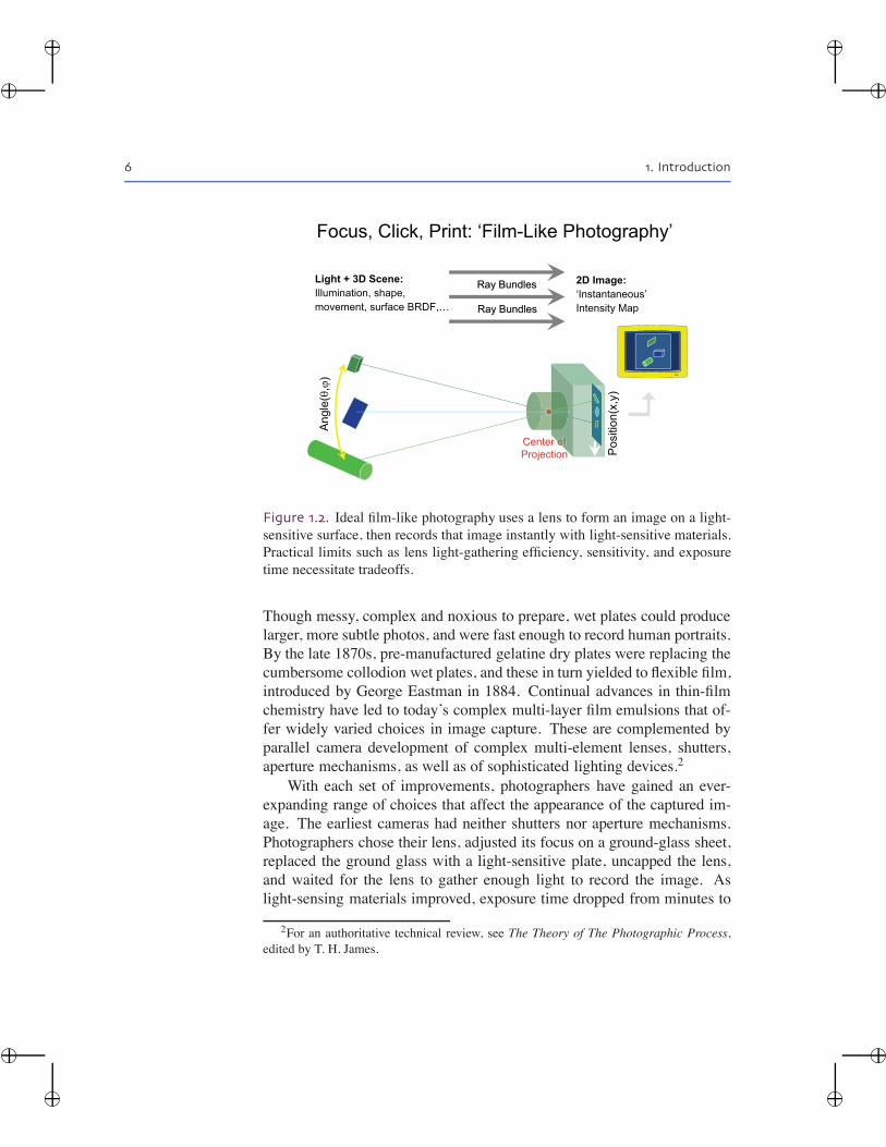
Focus, Click, Print: ‘Film-Like Photography’
2D Image:‘Instantaneous’Intensity Map
Light + 3D Scene:Illumination, shape, movement, surface BRDF,…
Ang
le(θ
,ϕ)
Pos
ition
(x,y
)
Center of Projection
of
Ray BundlesRay Bundles
Ray BundlesRay Bundles
Figure 1.2. Ideal film-like photography uses a lens to form an image on a light-sensitive surface, then records that image instantly with light-sensitive materials.Practical limits such as lens light-gathering efficiency, sensitivity, and exposuretime necessitate tradeoffs.
Though messy, complex and noxious to prepare, wet plates could producelarger, more subtle photos, and were fast enough to record human portraits.By the late 1870s, pre-manufactured gelatine dry plates were replacing thecumbersome collodion wet plates, and these in turn yielded to flexible film,introduced by George Eastman in 1884. Continual advances in thin-filmchemistry have led to today’s complex multi-layer film emulsions that of-fer widely varied choices in image capture. These are complemented byparallel camera development of complex multi-element lenses, shutters,aperture mechanisms, as well as of sophisticated lighting devices.2
With each set of improvements, photographers have gained an ever-expanding range of choices that affect the appearance of the captured im-age. The earliest cameras had neither shutters nor aperture mechanisms.Photographers chose their lens, adjusted its focus on a ground-glass sheet,replaced the ground glass with a light-sensitive plate, uncapped the lens,and waited for the lens to gather enough light to record the image. Aslight-sensing materials improved, exposure time dropped from minutes to
2For an authoritative technical review, see The Theory of The Photographic Process,edited by T. H. James.
�
�
�
�
�
�
�
�
1.3. Sampling the Dimensions of Imaging 7
seconds to milliseconds; adjustable-time shutters replaced lens caps; andadjustable lens apertures permitted regulation of the amount of light pass-ing through the lens during exposure. By the 1880s, the basic camerasettings were well-defined, and digital cameras have extended them onlyslightly. They are:
� Lens. Aperture, focusing distance, and focal length;
� Shutter. Exposure time;
� Sensor. Light sensitivity (film speed; ASA, ISO, or DIN) latitude(or tonal range or dynamic range), and color-sensing properties;
� Camera. Location, orientation, and the moment of exposure;
� Auxilliary lighting. Position, intensity, timing.
Most digital film-like cameras can automatically choose these settings.Once the shutter is tripped, these choices are fixed; the resultant image isone among many possible photographs. At the instant of the shutter-click,the camera has chosen the following settings:
(a) Field of view. The focal length of the lens determines the angularextent of the picture. A short (wide) focal length gives a wide-anglepicture; a long (telephoto) focal length gives a narrow one. Thoughthe image may be cropped later (at a corresponding loss of resolu-tion), it cannot be widened.
(b) Exposure and dynamic range. The chosen lens aperture, exposuretime, the sensors’ film speed (ISO, sensitivity), and its latitude to-gether determine how amounts of light in the scene map to picturevalues between black and white. Larger aperture settings, longerexposure times, or higher sensitivities map dimly-lit scenes to ac-ceptable pictures, while smaller apertures, shorter exposure times,and lower sensitivity will be chosen for brilliantly sun-lit scenes.Poor choices here may mean loss of visible details in too-bright ar-eas of the image, in too-dark areas, or both. Within the sensito-metric response curve of any sensor, the latitude of the film or thedynamic range of the sensor (the intensity ratio between the dark-est and lightest details) is not usually adjustable, and falls typicallybetween 200:1 to 1000:1.
�
�
�
�
�
�
�
�
8 1. Introduction
(c) Depth of field. The lens aperture focal length and sensor size to-gether determine how wide a range of distances will appear in fo-cus. A small aperture and short (wide) focal length gives the great-est depth of field, while large apertures with long focal lengths yieldnarrow ranges of focus.3 (Note that increased depth of field normallyrequire a smaller aperture, which may entail increased exposure timeor sensor sensitivity (which in turn increases noise).)
(d) Temporal resolution. The chosen exposure time determines howlong the camera will collect light for each point in the image. If theexposure time is too long, moving objects will appear blurred; if itis too short, the camera may not gather enough light for a properexposure.
(e) Spatial resolution. For a well-focused image, the sensor itself setsthe spatial resolution. It may be artificially blurred, but no sharpen-ing can recover more detail than that already recorded by the cam-era. Note that increased resolution reduces depth of focus and oftenincreases visible noise due to reduced sensor pixel size.
(f) Wavelength resolution. Color-balance and saturation settings onthe camera set sensitivity to color. Current film-like cameras sensecolor by measuring three primaries (usually R,G,B) with fixed, over-lapping spectral response curves. While different sensors (especiallyblack-and-white film stocks) offer varying spectral curves, none isadjustable.
In every case, film-like photography forces us to choose, to make trade-offs among interdependent parameters, and to lock in those choices in asingle photo at the moment we click the shutter. If we choose a long ex-posure time to gather enough light, movement in the scene may blur thepicture, while too short an exposure time in order to freeze motion maymake the picture too dark. We can keep the exposure time short if we in-crease the aperture size, but then we lose depth of focus, and foregroundor background objects are no longer sharp. We can increase the depthof focus again if we shorten (widen) the focal length and move closer tothe subject, but then we alter the foreshortening of the image. The basic
3Some portraits (e.g., Matthew Brady’s close-up photos of Abraham Lincoln show eyesin sharp focus but employ soft focus in other planes to hide blemishes elsewhere on theface.
�
�
�
�
�
�
�
�
1.3. Sampling the Dimensions of Imaging 9
“camera obscura” design of film-like photography forces these tradeoffs;they are inescapable due to the hard limits of simple image formation andthe measurement of light. We would like to capture any viewed scene, nomatter how transient and fast-moving in an infinitesimally short time pe-riod,; we would like to have the ability to choose any aperture, even a verytiny one in dim light; and we would like unbounded resolution that wouldallow capture of a very wide field of view. Unfortunately, this ideal cam-era’s infinitesimal aperture and zero-length exposure time would gather nophotons at all!
New methods of computational photography, however, offer a steadilygrowing number of ways to escape the bind of these tradeoffs, and gainnew capabilities. Existing film-like camera designs are already excellent;we have economical cameras that offer a tremendous adjustment range foreach of these parameters; We are increasingly confident of finding compu-tational strategies to untangle them.
1.3.2 Present: Epsilon Photography
Think of film cameras at their best as defining a “box” in the multi-dimensional space of imaging parameters. The first, most obvious thingwe can do to improve digital cameras is to expand this box in every con-ceivable dimension. The goal would be to build a super-camera that hasenhanced performance in terms of the traditional parameters, such as dy-namic range, field of view or depth of field. In this project of a super-camera, computational photography becomes “epsilon photography,” inwhich the scene is recorded via multiple images that vary at least one ofthe camera parameters by some small amount or epsilon. For example,successive images (or neighboring pixels) may have different settings forparameters such as exposure, focus, aperture, view, illumination, or timingof the instant of capture. Each setting allows recording of partial infor-mation about the scene, and the final image is reconstructed by combiningall the useful parts of these multiple observations. Epsilon photography isthus the concatenation of many such boxes in parameter space, i.e., mul-tiple film-style photos computationally merged to make a more completephoto or scene description. While the merged photo is superior, each of theindividual photos is still useful and comprehensible independently. Themerged photo contains the best features from of the group. Thus epsilonphotography corresponds to the low-level vision: estimating pixels andpixel features with the best signal-to-noise ratio.
�
�
�
�
�
�
�
�
10 1. Introduction
(a) Field of view. A wide field of view panorama is achieved by stitch-ing and mosaicking pictures taken by panning a camera around acommon center of projection or by translating a camera over a near-planar scene.
(b) Dynamic range. A high dynamic range image is captured by merg-ing photos at a series of exposure values.and Picard 93, Debevec andMalik 97, Kang et al. 03].
(c) Depth of field. An image entirely in focus, foreground to back-ground, is reconstructed from images taken by successively chang-ing the plane of focus [Agrawala et al 05].
(d) Spatial resolution. Higher resolution is achieved by tiling multiplecameras (and mosaicing individual images) [Wilburn et al. 05] or byjittering a single camera [Landolt et al. 01].
(e) Wavelength resolution. Conventional cameras sample only threebasis colors. But multi-spectral imaging (from multiple colors in thevisible spectrum) or hyper-spectral imaging (from wavelengths be-yond the visible spectrum) are accomplished by successively chang-ing color filters in front of the camera during exposure, using tunablewavelength filters or diffraction gratings [Mohan et al. 08].
(f) Temporal resolution. High-speed imaging is achieved by staggeringthe exposure time of multiple low-frame-rate cameras. The exposuredurations of individual cameras can be non-overlapping [Wilburn etal. 05] or overlaping [Shechtman et al 02].
Photographing multiple images under varying camera parameters canbe done in several ways. Images can be taken with a single camera overtime. Or, images can be captured simultaneously using “assorted pixels”where each pixel is tuned to a different value for a given parameter [Nayarand Narsimhan 2002]. Just as some early digital cameras captured scan-lines sequentially, including those that scanned a single one-dimensionaldetector array across the image plane, detectors are conceivable that in-tentionally randomize each pixel’s exposure time to trade off motion-blurand resolution, previously explored for interactive computer graphics ren-dering [Dayal 05]. Simultaneous capture of multiple samples can also berecorded using multiple cameras, each camera having different values for
�
�
�
�
�
�
�
�
1.3. Sampling the Dimensions of Imaging 11
a given parameter. Two designs are currently being employed for multi-camera solutions: a camera array [Wilburn et al. 05] and single-axis mul-tiple parameter (co-axial) cameras [Mcguire et al. 05].
1.3.3 Future: Coded Photography
But we wish to go far beyond the best possible film camera. Instead ofhigh quality pixels, the goal is to capture and convey the mid-level cues:shapes, boundaries, materials, and organization. Coded photography re-versibly encodes information about the scene in a single photograph (or avery few photographs) so that the corresponding decoding allows power-ful decomposition of the image into light fields, motion-resolved images,global/direct illumination components, or distinction between geometricversus material discontinuities.
Instead of increasing the field of view just by panning a camera, canwe also create a wrap-around view of an object? Panning a camera allowsus to concatenate and expand the box in the camera parameter space inthe dimension of field of view. But a wrap-around view spans multipledisjoint pieces along this dimension. We can virtualize the notion of thecamera itself if we consider it as a device for collecting bundles of raysleaving a viewed object in many directions, not just towards a single lens,and virtualize it further if we gather each ray with its own wavelengthspectrum.
Coded photography is a notion of an out-of-the-box photographicmethod, in which individual (ray) samples or data sets may not be compre-hensible as images without further decoding, re-binning or reconstruction.For example, a wrap-around view might be built from multiple imagestaken from a ring or a sphere of camera positions around the object, butthe view takes only a few pixels from each input image for the final result;could we find a better, less wasteful way to gather the pixels we need?Coded aperture techniques, inspired by work in astronomical imaging, tryto preserve the high spatial frequencies of light that passes through thelens so that out-of-focus blurred images can be digitally re-focused [Veer-araghavan 07] or resolved in depth [Levin07]. By coding illumination, itis possible to decompose radiance in a scene into direct and global com-ponents [Nayar06]. Using a coded exposure technique, the shutter of acamera can be rapidly fluttered open and closed in a carefully chosen bi-nary sequence as it captures a single photo. The fluttered shutter encodesthe motion that conventionally appears blurred in a reversible way; we cancompute a moving but un-blurred image. Other examples include confo-
�
�
�
�
�
�
�
�
12 1. Introduction
cal synthetic aperture imaging [Levoy 04] that lets us see through murkywater, and techniques to recover glare by capturing selected rays througha calibrated grid [Talvala 07]. What other novel abilities might be possi-ble by combining computation with sensing novel combinations of sceneappearance?
In fact,the next phase of computational photography will go beyond theradiometric quantities and challenge the notion that a synthesized photoshould appear to come from a device that mimics a single-chambered hu-man eye. Instead of recovering physical parameters, the goal will be tocapture the visual essence of the scene and scrutinize the perceptually crit-ical components. This essence photography may loosely resemble depic-tion of the world after high-level vision processing. In addition to photons,additional elements will sense location coordinates, identities, and gesturesvia novel probes and actuators. With sophisticated algorithms, we will ex-ploit priors based on natural image statistics and online community photocollections [Snavely 06, Hays 07]. Essence photography will spawn newforms of visual artistic expression and communication.
Wemay be converging on a new, much more capable box of parametersin computational photography that we can’t yet fully recognize; there isquite a bit of innovation yet to come!
�
�
�
�
�
�
�
�
Chapter 3
Extending Film-LikeDigital Photography
As a thought experiment, suppose we accept our existing film-like con-cepts of photography, just as they have stood for well over a century.For the space of this chapter, let’s continue to think of any and all pho-tographs, whether captured digitally or on film, as a fixed and static recordof a viewed scene, a straightforward copy of the 2D image formed on aplane behind a lens. How might we improve the results from these tra-ditional cameras and the photographs they produce if we could apply un-limited computing, storage, and communication to them? The past fewyears have yielded a wealth of new opportunities, as miniaturization al-lows lightweight battery-powered devices such as mobile phones to rivalthe computing power of the desktop machines of only a few years ago, andas manufacturers can produce millions of low-cost, low-power and com-pact digital image sensors, high-precision motorized lens systems, bright,full-color displays, and even palm-sized projectors, integrated into virtu-ally any form as low-priced products. How can these computing opportu-nities improve conventional forms of photography?
Currently, adjustments and tradeoffs dominate film-like photography,and most decisions are locked in once we press the camera’s shutter re-lease. Excellent photos are often the result of meticulous and artful adjust-ments, and the sheer number of adjustments has grown as digital cameraelectronics have replaced film chemistry, and now include ASA settings,tone scales, flash control, complex multi-zone light metering, color bal-
13
�
�
�
�
�
�
�
�
14 3. Extending Film-Like Digital Photography
ance, and color saturation. Yet we make all these adjustments before wetake the picture, and even our hastiest decisions are usually irreversible.Poor choices lead to poor photos, and an excellent photo may be possi-ble only for an exquisitely narrow combination of settings taken with ashutter-click at just the right moment. Can we elude these tradeoffs? Canwe defer choosing the camera’s settings somehow, or change our mindsand re-adjust them later? Can we compute new images that expand therange of settings, such as a month-long exposure time? What new flexibil-ities might allow us to take a better picture now, and also keep our choicesopen to create an even better one later?
3.1 Understanding Limitations
This is a single-strategy chapter. As existing digital cameras are alreadyextremely capable and inexpensive, here we will explore different ways toconstruct combined results from multiple cameras and/or multiple images.By digitally combining the information from more than one image, we cancompute a picture superior to what any single camera could produce andmay also create interactive display applications that let users adjust andexplore settings that were fixed in film-like photography.1
This strategy is a generalization of bracketing already familiar to mostphotographers. Bracketing lets photographers avoid uncertainty about crit-ical camera settings such as focus or exposure; instead of taking just onephoto at what we think are the correct settings, we make additional expo-sures at several higher and lower settings that bracket the chosen one. Ifour first, best-guess setting was not the correct choice, the bracketed set ofphotos almost always contains a better one. The methods in this chapterare analogous, but often use a larger set of photos as multiple settings may
1For example, HDRShop from Paul Debevec’s research group at USC-ICT (http://projects.ict.usc.edu/graphics/HDRShop) helps users construct high-dynamic-range imagesfrom bracketed-exposure image sets, then lets users interactively adjust exposure settings toreveal details in brilliant highlights or the darkest shadows; Autostitch from David Lowe’sgroup at UBC (http://www.cs.ubc.ca/∼mbrown/autostitch/autostitch.html) and AutoPano-SIFT (http://user.cs.tu-berlin.de/∼nowozin/autopano-sift/) let users construct cylindrical orspherical panoramas from overlapped images; and HD View from Microsoft Research(http://research.microsoft.com/ivm/hdview.htm) allows users an extreme form of zoom toexplore high-resolution panoramas, varying smoothly from spherical projections for verywide-angle views (e.g., > 180 degrees) to planar projections for very narrow, telescopicviews (< 1 degree).
�
�
�
�
�
�
�
�
3.1. Understanding Limitations 15
be changed, and we may digitally merge desirable features from multipleimages in the set rather than simply select just one single best photo.
We need to broaden our thinking about photography to avoid missingsome opportunities. So many of the limitations and trade-offs of traditionalphotography have been with us for so long that we tend to assume they are
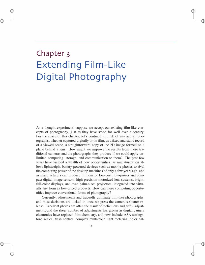
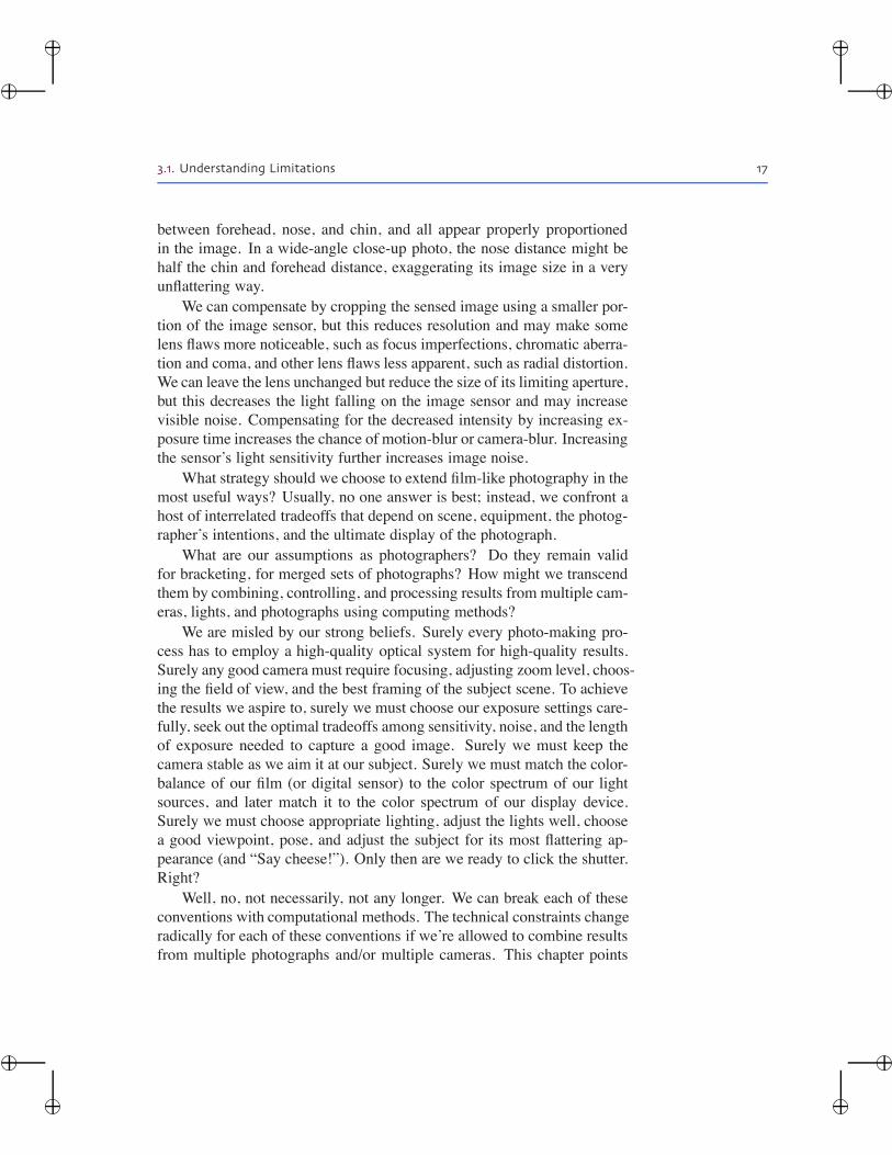
Figure 3.1. No physically realizable lens could achieve enough depth-of-fieldfor this insect closeup: we can focus on antennae or thorax or in-between (top).However, with a large enough series of bracketed focus images and the right formsof optimization, we can assemble an “all-focus” image (bottom) from the bestparts of each photo. (Image Credits: Digital Photomontage [Agrawal04]).
�
�
�
�
�
�
�
�
16 3. Extending Film-Like Digital Photography
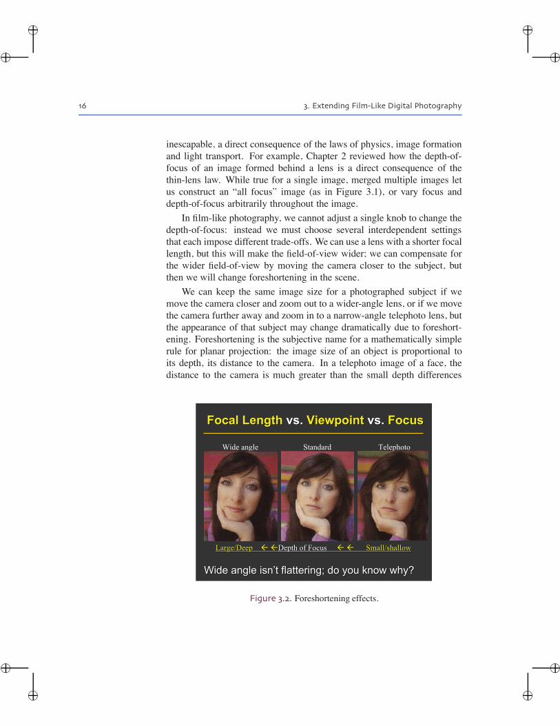
inescapable, a direct consequence of the laws of physics, image formationand light transport. For example, Chapter 2 reviewed how the depth-of-focus of an image formed behind a lens is a direct consequence of thethin-lens law. While true for a single image, merged multiple images letus construct an “all focus” image (as in Figure 3.1), or vary focus anddepth-of-focus arbitrarily throughout the image.
In film-like photography, we cannot adjust a single knob to change thedepth-of-focus: instead we must choose several interdependent settingsthat each impose different trade-offs. We can use a lens with a shorter focallength, but this will make the field-of-view wider; we can compensate forthe wider field-of-view by moving the camera closer to the subject, butthen we will change foreshortening in the scene.
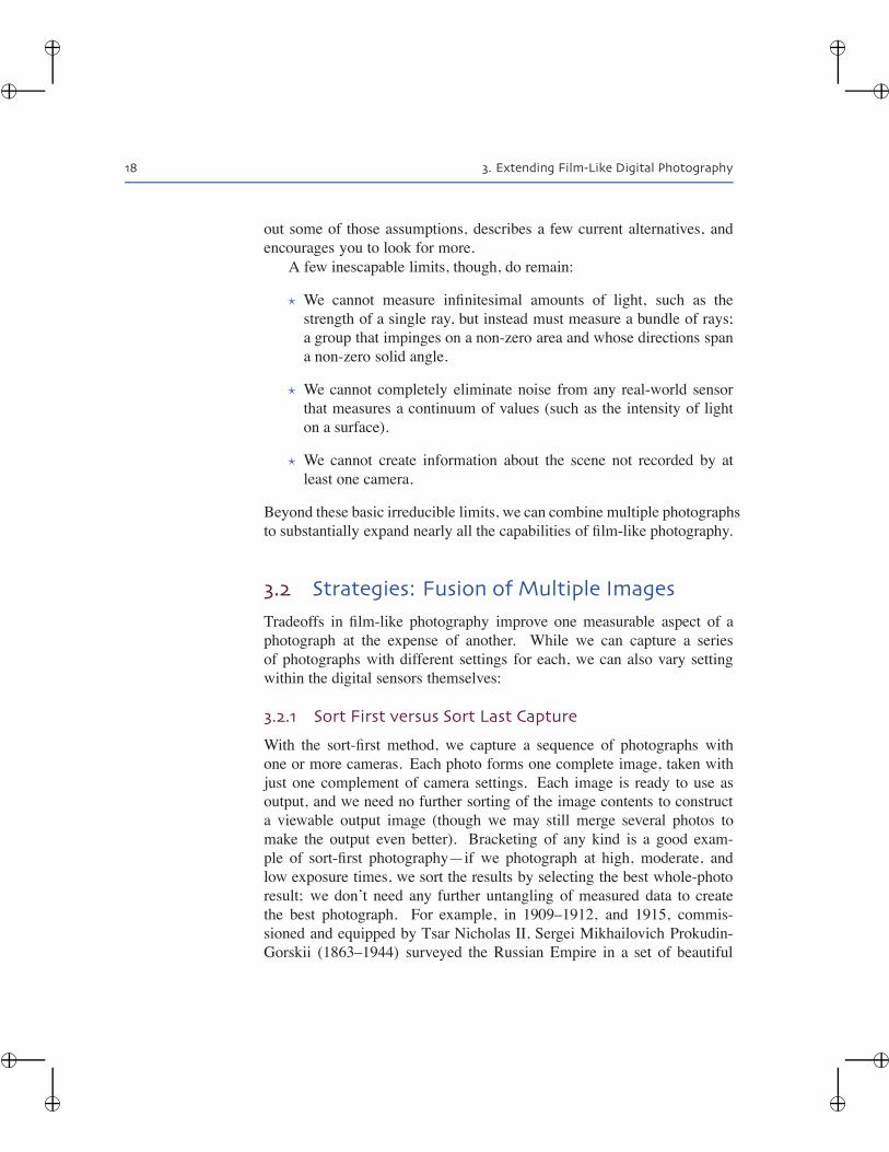
We can keep the same image size for a photographed subject if wemove the camera closer and zoom out to a wider-angle lens, or if we movethe camera further away and zoom in to a narrow-angle telephoto lens, butthe appearance of that subject may change dramatically due to foreshort-ening. Foreshortening is the subjective name for a mathematically simplerule for planar projection: the image size of an object is proportional toits depth, its distance to the camera. In a telephoto image of a face, thedistance to the camera is much greater than the small depth differences
Focal Length vs. Viewpoint vs. FocusFocal Length Focal Length vs. vs. Viewpoint Viewpoint vs.vs. FocusFocus
Wide angle isnWide angle isn’’t flattering; do you know why?t flattering; do you know why?
Wide angle Standard Telephoto
Large/Deep Large/Deep �� ��Depth of FocusDepth of Focus �� �� Small/shallowSmall/shallow
Figure 3.2. Foreshortening effects.
�
�
�
�
�
�
�
�
3.1. Understanding Limitations 17
between forehead, nose, and chin, and all appear properly proportionedin the image. In a wide-angle close-up photo, the nose distance might behalf the chin and forehead distance, exaggerating its image size in a veryunflattering way.
We can compensate by cropping the sensed image using a smaller por-tion of the image sensor, but this reduces resolution and may make somelens flaws more noticeable, such as focus imperfections, chromatic aberra-tion and coma, and other lens flaws less apparent, such as radial distortion.We can leave the lens unchanged but reduce the size of its limiting aperture,but this decreases the light falling on the image sensor and may increasevisible noise. Compensating for the decreased intensity by increasing ex-posure time increases the chance of motion-blur or camera-blur. Increasingthe sensor’s light sensitivity further increases image noise.
What strategy should we choose to extend film-like photography in themost useful ways? Usually, no one answer is best; instead, we confront ahost of interrelated tradeoffs that depend on scene, equipment, the photog-rapher’s intentions, and the ultimate display of the photograph.
What are our assumptions as photographers? Do they remain validfor bracketing, for merged sets of photographs? How might we transcendthem by combining, controlling, and processing results from multiple cam-eras, lights, and photographs using computing methods?
We are misled by our strong beliefs. Surely every photo-making pro-cess has to employ a high-quality optical system for high-quality results.Surely any good camera must require focusing, adjusting zoom level, choos-ing the field of view, and the best framing of the subject scene. To achievethe results we aspire to, surely we must choose our exposure settings care-fully, seek out the optimal tradeoffs among sensitivity, noise, and the lengthof exposure needed to capture a good image. Surely we must keep thecamera stable as we aim it at our subject. Surely we must match the color-balance of our film (or digital sensor) to the color spectrum of our lightsources, and later match it to the color spectrum of our display device.Surely we must choose appropriate lighting, adjust the lights well, choosea good viewpoint, pose, and adjust the subject for its most flattering ap-pearance (and “Say cheese!”). Only then are we ready to click the shutter.Right?
Well, no, not necessarily, not any longer. We can break each of theseconventions with computational methods. The technical constraints changeradically for each of these conventions if we’re allowed to combine resultsfrom multiple photographs and/or multiple cameras. This chapter points
�
�
�
�
�
�
�
�
18 3. Extending Film-Like Digital Photography
out some of those assumptions, describes a few current alternatives, andencourages you to look for more.
A few inescapable limits, though, do remain:
� We cannot measure infinitesimal amounts of light, such as thestrength of a single ray, but instead must measure a bundle of rays;a group that impinges on a non-zero area and whose directions spana non-zero solid angle.
� We cannot completely eliminate noise from any real-world sensorthat measures a continuum of values (such as the intensity of lighton a surface).
� We cannot create information about the scene not recorded by atleast one camera.
Beyond these basic irreducible limits, we can combine multiple photographsto substantially expand nearly all the capabilities of film-like photography.
3.2 Strategies: Fusion of Multiple Images
Tradeoffs in film-like photography improve one measurable aspect of aphotograph at the expense of another. While we can capture a seriesof photographs with different settings for each, we can also vary settingwithin the digital sensors themselves:
3.2.1 Sort First versus Sort Last Capture
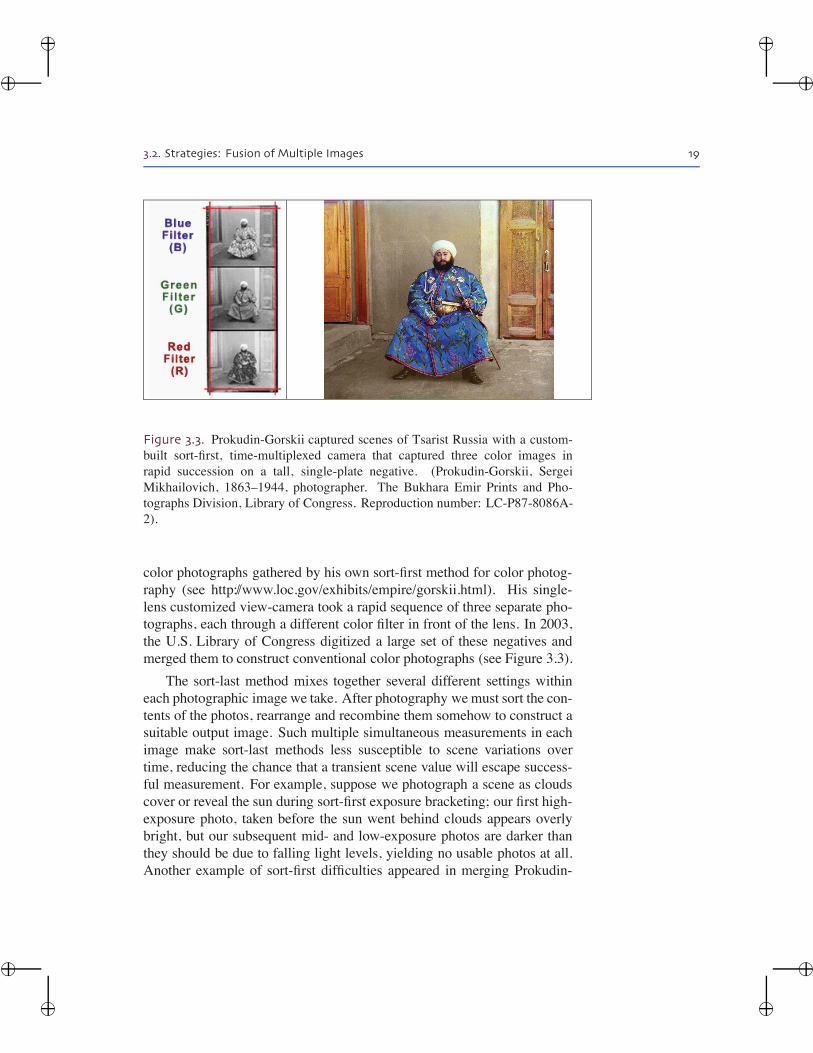
With the sort-first method, we capture a sequence of photographs withone or more cameras. Each photo forms one complete image, taken withjust one complement of camera settings. Each image is ready to use asoutput, and we need no further sorting of the image contents to constructa viewable output image (though we may still merge several photos tomake the output even better). Bracketing of any kind is a good exam-ple of sort-first photography—if we photograph at high, moderate, andlow exposure times, we sort the results by selecting the best whole-photoresult; we don’t need any further untangling of measured data to createthe best photograph. For example, in 1909–1912, and 1915, commis-sioned and equipped by Tsar Nicholas II, Sergei Mikhailovich Prokudin-Gorskii (1863–1944) surveyed the Russian Empire in a set of beautiful
�
�
�
�
�
�
�
�
3.2. Strategies: Fusion of Multiple Images 19
Figure 3.3. Prokudin-Gorskii captured scenes of Tsarist Russia with a custom-built sort-first, time-multiplexed camera that captured three color images inrapid succession on a tall, single-plate negative. (Prokudin-Gorskii, SergeiMikhailovich, 1863–1944, photographer. The Bukhara Emir Prints and Pho-tographs Division, Library of Congress. Reproduction number: LC-P87-8086A-2).
color photographs gathered by his own sort-first method for color photog-raphy (see http://www.loc.gov/exhibits/empire/gorskii.html). His single-lens customized view-camera took a rapid sequence of three separate pho-tographs, each through a different color filter in front of the lens. In 2003,the U.S. Library of Congress digitized a large set of these negatives andmerged them to construct conventional color photographs (see Figure 3.3).
The sort-last method mixes together several different settings withineach photographic image we take. After photography wemust sort the con-tents of the photos, rearrange and recombine them somehow to construct asuitable output image. Such multiple simultaneous measurements in eachimage make sort-last methods less susceptible to scene variations overtime, reducing the chance that a transient scene value will escape success-ful measurement. For example, suppose we photograph a scene as cloudscover or reveal the sun during sort-first exposure bracketing; our first high-exposure photo, taken before the sun went behind clouds appears overlybright, but our subsequent mid- and low-exposure photos are darker thanthey should be due to falling light levels, yielding no usable photos at all.Another example of sort-first difficulties appeared in merging Prokudin-
�
�
�
�
�
�
�
�
20 3. Extending Film-Like Digital Photography
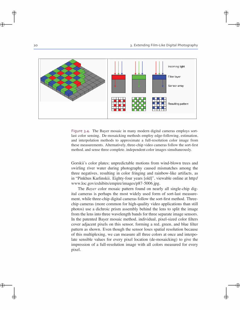
Figure 3.4. The Bayer mosaic in many modern digital cameras employs sort-last color sensing. De-mosaicking methods employ edge-following, estimation,and interpolation methods to approximate a full-resolution color image fromthese measurements. Alternatively, three-chip video cameras follow the sort-firstmethod, and sense three complete, independent color images simultaneously.
Gorskii’s color plates; unpredictable motions from wind-blown trees andswirling river water during photography caused mismatches among thethree negatives, resulting in color fringing and rainbow-like artifacts, asin “Pinkhus Karlinskii. Eighty-four years [old]”, viewable online at http://www.loc.gov/exhibits/empire/images/p87-5006.jpg.
The Bayer color mosaic pattern found on nearly all single-chip dig-ital cameras is perhaps the most widely used form of sort-last measure-ment, while three-chip digital cameras follow the sort-first method. Three-chip cameras (more common for high-quality video applications than stillphotos) use a dichroic prism assembly behind the lens to split the imagefrom the lens into three wavelength bands for three separate image sensors.In the patented Bayer mosaic method, individual, pixel-sized color filterscover adjacent pixels on this sensor, forming a red, green, and blue filterpattern as shown. Even though the sensor loses spatial resolution becauseof this multiplexing, we can measure all three colors at once and interpo-late sensible values for every pixel location (de-mosaicking) to give theimpression of a full-resolution image with all colors measured for everypixel.
�
�
�
�
�
�
�
�
3.2. Strategies: Fusion of Multiple Images 21
3.2.2 Time- and Space-Multiplexed Capture
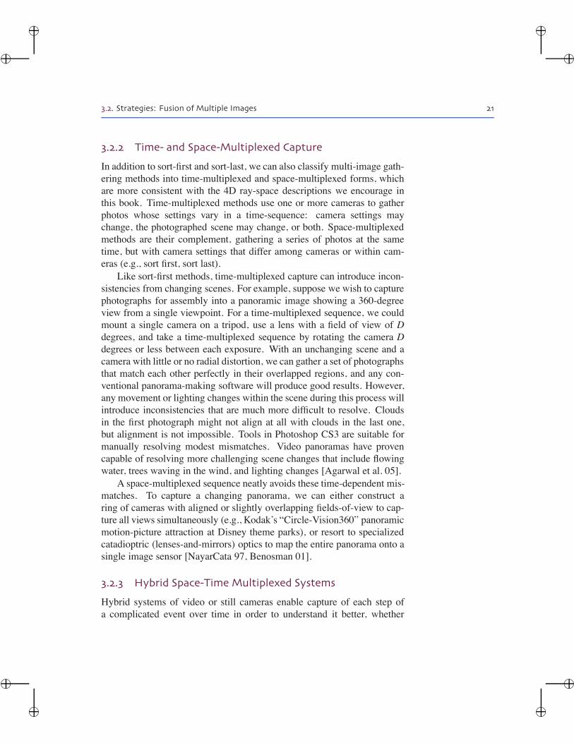
In addition to sort-first and sort-last, we can also classify multi-image gath-ering methods into time-multiplexed and space-multiplexed forms, whichare more consistent with the 4D ray-space descriptions we encourage inthis book. Time-multiplexed methods use one or more cameras to gatherphotos whose settings vary in a time-sequence: camera settings maychange, the photographed scene may change, or both. Space-multiplexedmethods are their complement, gathering a series of photos at the sametime, but with camera settings that differ among cameras or within cam-eras (e.g., sort first, sort last).
Like sort-first methods, time-multiplexed capture can introduce incon-sistencies from changing scenes. For example, suppose we wish to capturephotographs for assembly into a panoramic image showing a 360-degreeview from a single viewpoint. For a time-multiplexed sequence, we couldmount a single camera on a tripod, use a lens with a field of view of Ddegrees, and take a time-multiplexed sequence by rotating the camera Ddegrees or less between each exposure. With an unchanging scene and acamera with little or no radial distortion, we can gather a set of photographsthat match each other perfectly in their overlapped regions, and any con-ventional panorama-making software will produce good results. However,any movement or lighting changes within the scene during this process willintroduce inconsistencies that are much more difficult to resolve. Cloudsin the first photograph might not align at all with clouds in the last one,but alignment is not impossible. Tools in Photoshop CS3 are suitable formanually resolving modest mismatches. Video panoramas have provencapable of resolving more challenging scene changes that include flowingwater, trees waving in the wind, and lighting changes [Agarwal et al. 05].
A space-multiplexed sequence neatly avoids these time-dependent mis-matches. To capture a changing panorama, we can either construct aring of cameras with aligned or slightly overlapping fields-of-view to cap-ture all views simultaneously (e.g., Kodak’s “Circle-Vision360” panoramicmotion-picture attraction at Disney theme parks), or resort to specializedcatadioptric (lenses-and-mirrors) optics to map the entire panorama onto asingle image sensor [NayarCata 97, Benosman 01].
3.2.3 Hybrid Space-Time Multiplexed Systems
Hybrid systems of video or still cameras enable capture of each step ofa complicated event over time in order to understand it better, whether
�
�
�
�
�
�
�
�
22 3. Extending Film-Like Digital Photography
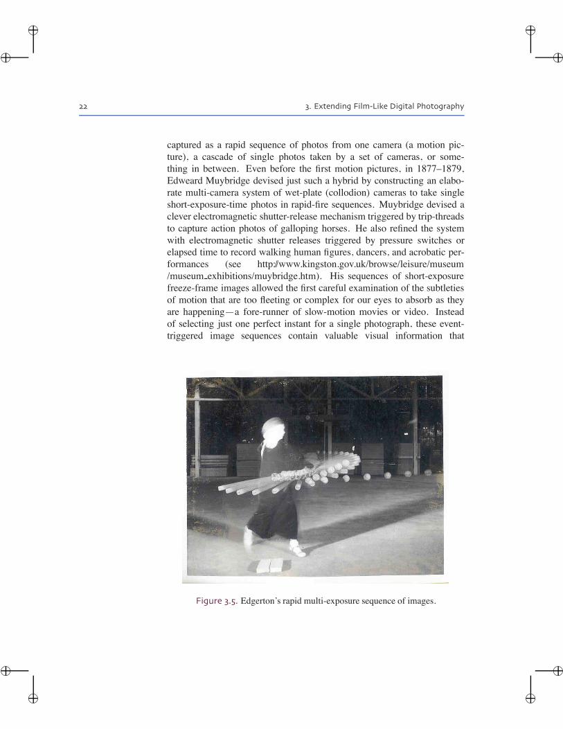
captured as a rapid sequence of photos from one camera (a motion pic-ture), a cascade of single photos taken by a set of cameras, or some-thing in between. Even before the first motion pictures, in 1877–1879,Edweard Muybridge devised just such a hybrid by constructing an elabo-rate multi-camera system of wet-plate (collodion) cameras to take singleshort-exposure-time photos in rapid-fire sequences. Muybridge devised aclever electromagnetic shutter-release mechanism triggered by trip-threadsto capture action photos of galloping horses. He also refined the systemwith electromagnetic shutter releases triggered by pressure switches orelapsed time to record walking human figures, dancers, and acrobatic per-formances (see http://www.kingston.gov.uk/browse/leisure/museum/museum exhibitions/muybridge.htm). His sequences of short-exposurefreeze-frame images allowed the first careful examination of the subtletiesof motion that are too fleeting or complex for our eyes to absorb as theyare happening—a fore-runner of slow-motion movies or video. Insteadof selecting just one perfect instant for a single photograph, these event-triggered image sequences contain valuable visual information that
Figure 3.5. Edgerton’s rapid multi-exposure sequence of images.
�
�
�
�
�
�
�
�
3.2. Strategies: Fusion of Multiple Images 23
stretches across time and across a sequence of camera positions and issuitable for several different kinds of computational merging.
Perhaps the simplest computational merging of time-multiplexed im-ages occurs within the camera itself. In his seminal work on fast, high-powered electronic (Xenon) strobe lights, Harold Edgerton showed thata rapid multiple-exposure sequence can be as revealing as a high-speedmotion-picture sequence (see Figure 3.5).
In addition to its visual interest, photos lit by a precisely timed strobesequence like this permit easy frame-to-frame measurements. For exam-ple, Figure 3.5 confirms that baseballs follow elastic collision dynamics.2
In some of Muybridge’s pioneering efforts, two or more cameras weretriggered at once to capture multiple views simultaneously. Modern workby Bregler and others on motion-capture from video merged these earlymulti-view image sequences computationally to infer the 3D shapes andthe movements that caused them. By finding image regions undergoingmovements consistent with rigid jointed 3D shapes in each image set, Bre-gler et al. could compute detailed estimates of the 3D position of eachbody segment in each frame and re-render the image sets as short moviesat any frame rate viewed from any desired viewpoint [Bregler et al. 98].
In another ambitious experiment, at Stanford University, more thanone hundred years after Muybridge’s work, Marc Levoy and colleaguesconstructed an adaptable array of 128 individual film-like digital videocameras that perform both time-multiplexed and space-multiplexed imagecapture simultaneously [Wilburn 05]. The reconfigurable array enabled awide range of computational photography experiments. Built on lessonsfrom earlier arrays (e.g., [Kanade 97, Yang 02, Matusik 04, Zhang 04]),the system’s interchangeable lenses, custom control hardware, and refinedmounting system permitted adjustment of camera optics, positioning, aim-ing, arrangement, and spacing between cameras. One configuration keptthe cameras packed together, just one inch apart, and staggered the trig-gering times for each camera within the normal 1/30 second video frameinterval. The video cameras all viewed the same scene from almost thesame viewpoint, but each viewed the scene during different overlappedtime periods. By assembling the differences between overlapped videoframes from different cameras, the team was able to compute the output ofa virtual high-speed camera running at multiples of the individual cameraframe rates and as high as 3,000 frames per second.
2Similarly, you can try your own version of Edgerton’s well-known milk-drop photosequences (with a digital flash camera, an eye dropper, and a bowl of milk.
�
�
�
�
�
�
�
�
24 3. Extending Film-Like Digital Photography
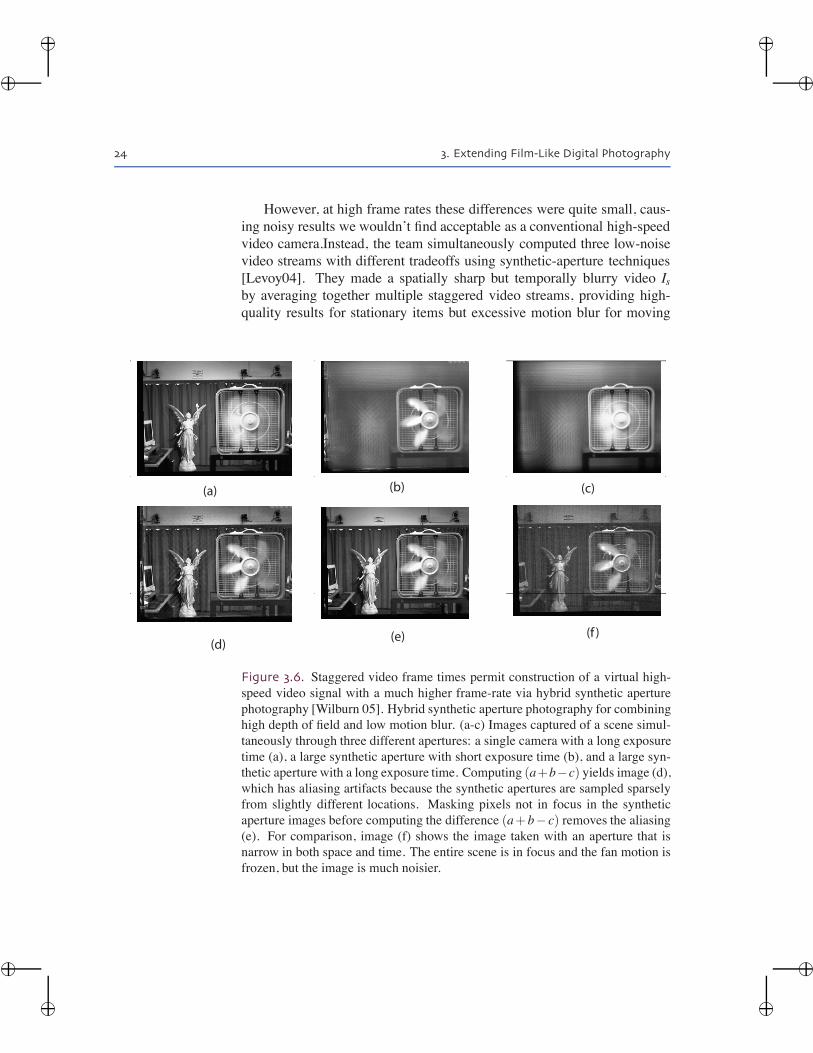
However, at high frame rates these differences were quite small, caus-ing noisy results we wouldn’t find acceptable as a conventional high-speedvideo camera.Instead, the team simultaneously computed three low-noisevideo streams with different tradeoffs using synthetic-aperture techniques[Levoy04]. They made a spatially sharp but temporally blurry video Is
by averaging together multiple staggered video streams, providing high-quality results for stationary items but excessive motion blur for moving
(a) (b) (c)
(d) (e) (f )
Figure 3.6. Staggered video frame times permit construction of a virtual high-speed video signal with a much higher frame-rate via hybrid synthetic aperturephotography [Wilburn 05]. Hybrid synthetic aperture photography for combininghigh depth of field and low motion blur. (a-c) Images captured of a scene simul-taneously through three different apertures: a single camera with a long exposuretime (a), a large synthetic aperture with short exposure time (b), and a large syn-thetic aperture with a long exposure time. Computing (a+b−c) yields image (d),which has aliasing artifacts because the synthetic apertures are sampled sparselyfrom slightly different locations. Masking pixels not in focus in the syntheticaperture images before computing the difference (a+b− c) removes the aliasing(e). For comparison, image (f) shows the image taken with an aperture that isnarrow in both space and time. The entire scene is in focus and the fan motion isfrozen, but the image is much noisier.
�
�
�
�
�
�
�
�
3.3. Improving Dynamic Range 25
objects. For a temporally sharp video It , they averaged together spatialneighborhoods within each video frame to eliminate motion blur, but thisinduced excessive blur in stationary objects. They also computed a tempo-rally and spatially blurred video stream Iw, to hold the joint low-frequencyterms, so that the combined streams Is + It Iw exhibited reduced noise, sharpstationary features, and modest motion blur, as shown in Figure 3.6.
3.3 Improving Dynamic Range
Like any sensor, digital cameras have a limited input range: too muchlight dazzles the sensor, ruining the image with a featureless white glare,while too little light makes image features indistinguishable from perfectdarkness. How can that range be improved, allowing our cameras to seedetails in the darkest shadows and brightest highlights?
Film-like cameras provide several mechanisms to match the camera’soverall light sensitivity to the amount of light in a viewed scene, and digitalcameras can adjust most of them automatically. These include adjustingthe aperture size to limit the light admitted through the lens (though thisalters the depth-of-field), adjusting exposure time (though this may allowmotion blur), placing “neutral density” filters in the light-path (though thismight accidentally displace the camera), or adjusting the sensitivity of thesensor itself—using a film with a different ASA rating (which changesfilm-grain size), or changing the gain-equivalent settings on a digital cam-era (which changes the amount of noise). Despite their tradeoffs, thesemechanisms combine to give modern camera sensitivity an astoundinglywide sensitivity range, one that can rival or exceed that of the human eye,which adapts to sense light over 16 decades of intensity from the absolutethreshold of vision at about 10−6cd/m2 up to the threshold of light-inducedeye damage near 108cd/m2.
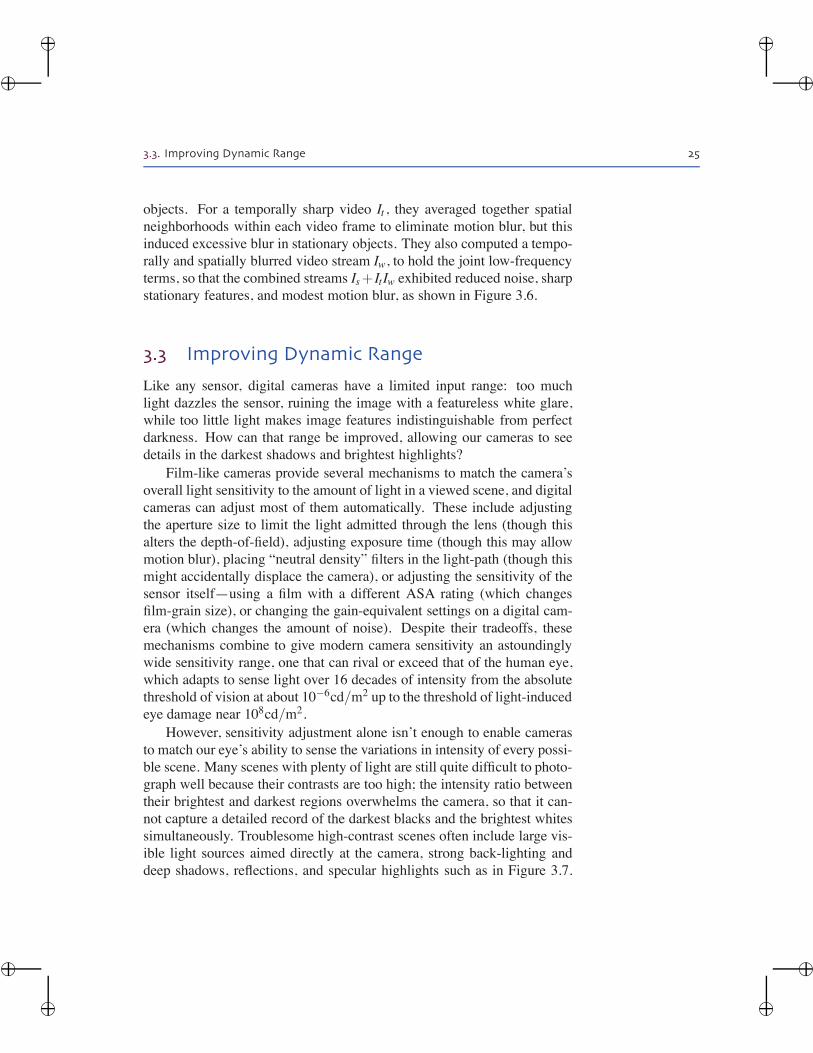
However, sensitivity adjustment alone isn’t enough to enable camerasto match our eye’s ability to sense the variations in intensity of every possi-ble scene. Many scenes with plenty of light are still quite difficult to photo-graph well because their contrasts are too high; the intensity ratio betweentheir brightest and darkest regions overwhelms the camera, so that it can-not capture a detailed record of the darkest blacks and the brightest whitessimultaneously. Troublesome high-contrast scenes often include large vis-ible light sources aimed directly at the camera, strong back-lighting anddeep shadows, reflections, and specular highlights such as in Figure 3.7.
�
�
�
�
�
�
�
�
26 3. Extending Film-Like Digital Photography
Figure 3.7. Tone-mapped HDR (high dynamic range) image from [Choud 03].Many back-lit scenes such as this one can easily exceed the dynamic range of mostcameras. Bottom row shows the original scene intensities scaled by progressivefactors of ten; note that scene intensities in the back-lit cloud regions at left areapproximately 10,000 times higher than shadowed forest details, well beyond the1000:1 dynamic range typical of conventional CMOS or CCD camera sensors.
Film-like photography offers us little recourse other than to add light to theshadowy regions with flash or fill-lighting; rather than adjust the camera tosuit the scene, we adjust the scene to suit the camera!
Unlike its sensitivity, the camera’s maximum contrast ratio, known asits dynamic range is not adjustable. Formally, it is the ratio between thebrightest and darkest light intensities a camera can capture from a scenewithin a single image without losing its detail-sensing abilities—the max-imum intensity ratio between the darkest detailed shadows and brightest
�
�
�
�
�
�
�
�
3.3. Improving Dynamic Range 27
textured brilliance, as shown in Figure 3.7. No one single sensitivitysetting (or exposure value) will suffice to capture a high dynamic range(HDR) scene that exceeds the camera’s contrast-sensingability.
Lens and sensor together limit the camera’s dynamic range. In a high-contrast scene, glare effects and unwanted light scattering within complexlens structures cause glare and flare effects that depend on the image it-self and cause traces of light from bright parts of the scene to “leak” intodark image areas, washing out shadow details and limiting the maximumcontrast the lens can form on the image on the sensor, typically between100,000:1 to 10 million to 1 [McCann 07, Levoy 07]. The sensor’s dy-namic range (typically < 1000 : 1) imposes further limits. Device elec-tronics (e.g., charge transfer rates) typically set the upper bound on theamount of sensed light, and the least amount of light distinguishable fromdarkness is set by both the sensor’s sensitivity and its noise floor,, the com-bined effect of all the camera’s noise sources (quantization, fixed-pattern,thermal, EMI/RFI, and photon arrival noise).
The range of visible intensities dwarfs the contrast abilities of cam-eras and displays. When plotted on a logarithmic scale (where distancedepicts ratios; each tic marks a factor-of-10 change), the range of humanvision spans about 16 decades, but typical film-like cameras and displaysspan no more than 2–3 decades. For the daylight-to-dusk (photopic) inten-sities (upper 2/3rds of scale), humans can detect some contrasts as smallas 1-2% (1.02:1, which divides a decade into 116 levels (1/log101.02)).Accordingly, 8-bit image quantization is barely adequate for cameras anddisplays whose dynamic range may exceed 2 decades (100:1); many use10, 12, or 14-bit internal representations to avoid visible contouring arti-facts.
3.3.1 Capturing High Dynamic Range
Film-like photography is frustrating for high-contrast scenes because eventhe most careful bracketing of camera-sensitivity settings will not allow usto capture the whole scene’s visible contents in a single picture. Sensi-tivity set high enough to reveal the shadow details will cause severe over-exposure for dark parts of the scene; sensitivity set low enough to capturevisible details in the brightest scene portions are far too low to capture anyvisible features in the dark parts of the image. However, several practicalmethods are available that let us capture all the scene contents in a usableway.
�
�
�
�
�
�
�
�
28 3. Extending Film-Like Digital Photography
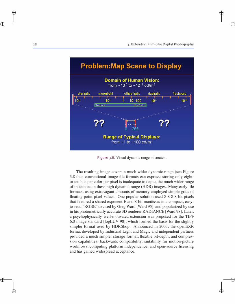
Figure 3.8. Visual dynamic range mismatch.
The resulting image covers a much wider dynamic range (see Figure3.8 than conventional image file formats can express; storing only eight-or ten bits per color per pixel is inadequate to depict the much wider rangeof intensities in these high dynamic range (HDR) images. Many early fileformats, using extravagant amounts of memory employed simple grids offloating-point pixel values. One popular solution used 8-8-8-8 bit pixelsthat featured a shared exponent E and 8-bit mantissas in a compact, easy-to-read “RGBE” devised by Greg Ward [Ward 95], and popularized by usein his photometrically accurate 3D renderer RADIANCE [Ward 98]. Later,a psychophysically well-motivated extension was proposed for the TIFF6.0 image standard [logLUV 98], which formed the basis for the slightlysimpler format used by HDRShop. Announced in 2003, the openEXRformat developed by Industrial Light and Magic and independent partnersprovided a much simpler storage format, flexible bit-depth, and compres-sion capabilities, backwards compatibility, suitability for motion-pictureworkflows, computing platform independence, and open-source licensingand has gained widespread acceptance.
�
�
�
�
�
�
�
�
3.3. Improving Dynamic Range 29
3.3.2 HDR by Multiple Exposures
The sort-first approach is very suitable for capturing HDR images. To cap-ture the finely-varied intensities in a high dynamic range scene, we cancapture multiple images using a motionless camera that takes perfectlyaligned images with different exposure settings and then merge these im-ages. In principle, the merge is simple; we divide the pixel value of eachpixel by the light sensitivity of the camera as it took that picture, and com-bine the best estimates of scene radiance at that pixel for all pictures wetook, ignoring badly over-and under-exposed images.
This simple form of merging is quick to compute and has found wide-spread early use as exposure bracketing [Morimura 93, Burt and Kol-czynski 93, Madden 93, Tsai 94], but many methods assumed the linearcamera response curves found on instrumentation cameras. Most dig-ital cameras intended for photography introduce intentional nonlineari-ties in their light response, often mimicking the s-shaped response curvesof film when plotted on log-log axes (H-D or Hurter-Driffield curves).These curves enable cameras to capture a wider usable range of inten-sities and provide a visually pleasing response to HDR scenes, retain-ing weak ability to capture intensity changes even at their extremes ofover- and under-exposure, and varying among different cameras. Someauthors have proposed the use of images acquired with different exposuresto estimate the radiometric response function of an imaging device anduse the estimated response function to process the images before mergingthem [Mann and Picard 95, Debevec and Malik 97, Mitsunaga and Nayar99]. This approach has proven robust and is now widely available in bothcommercial software tools (Adobe Photoshop CS2 and later, CinePaint)and open-source projects (HDRShop (http://www.hdrshop.com/), PFStools(http://www.mpi-inf.mpg.de/resources/pfstools/), and others).
3.3.3 HDR by Exotic Image Sensors
While quite easy and popular for static scenes, exposure-time bracketingmethods is not the only option available for capturing HDR scenes, andit is, moreover, unsuitable for scenes that vary rapidly over time. In laterchapters we will explore exotic image sensor designs that can sense higherdynamic range in a single exposure. They include logarithmic sensors,pixels with assorted attenuation [Nayar and Narsihman 03], multiple sen-sor designs with beam-splitters, gradient-measuring sensors [Tumblin etal. 05]. In addition, we will explore techniques for dealing with high dy-
�
�
�
�
�
�
�
�
30 3. Extending Film-Like Digital Photography
namic range scenes with video cameras [Kang et al. 05] or for capturingpanoramas with panning cameras via attenuating ramp filters [Ahuja etal. 02, Nayar et al. 02].
3.4 Beyond Tri-Color Sensing
At first glance an increase in the spectral resolution of camera, lights, andprojectors might not seem to offer any significant advantages in photog-raphy. Existing photographic methods quite sensibly rely on the well-established trichromatic response of human vision, and use three or morefixed color primaries such as red, green, and blue (RGB) to represent anycolor in the color gamut of the device.
Fixed-spectrum photography limits our ability to detect or depict sev-eral kinds of visually useful spectral differences. In the common phenom-ena of metamerism, the spectrum of available lighting used to view orphotograph objects can cause materials with notably different reflectancespectra to have the same apparent color because they evoke equal responsesfrom the broad, fixed color primaries in our eyes or the camera. Metamersare commonly observed in fabric dyes where two pieces of fabric mightappear to have the same color under one light source, and a very differentcolor under another.
Fixed color primaries also impose a hard limit on the gamut of colorsthat the device can accurately capture or reproduce. As demonstrated inthe CIE 1931 color space chromaticity diagram, each set of fixed colorprimaries defines a convex hull of perceived colors within the space of allhumanly perceptible colors. The device can reliably and accurately repro-duce only the colors inside the convex hull defined by its color primaries.In most digital cameras, the Bayer grid of fixed, passive R, G, B filtersoverlaid on pixel detectors set the color primaries. Current DMD projec-tors use broad-band light sources passed through a spinning wheel thatholds similar passive R, G, B filters. These filters compromise betweennarrow spectra that provide a large color gamut and broad spectra that pro-vide greatest on-screen brightness.
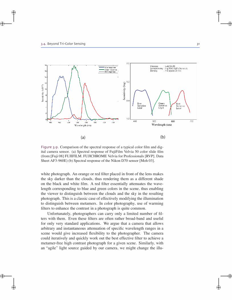
3.4.1 Metamers and Contrast Enhancement
Photographers often use yellow, orange, red, and green filters for variouseffects in black and white photography. For example, white clouds andblue sky are often rendered as roughly the same intensity in a black and
�
�
�
�
�
�
�
�
3.4. Beyond Tri-Color Sensing 31
(a) (b)
Figure 3.9. Comparison of the spectral response of a typical color film and dig-ital camera sensor. (a) Spectral response of FujiFilm Velvia 50 color slide film(from:[Fuji 08] FUJIFILM. FUJICHROME Velvia for Professionals [RVP]. DataSheet AF3-960E) (b) Spectral response of the Nikon D70 sensor [Moh 03].
white photograph. An orange or red filter placed in front of the lens makesthe sky darker than the clouds, thus rendering them as a different shadeon the black and white film. A red filter essentially attenuates the wave-length corresponding to blue and green colors in the scene, thus enablingthe viewer to distinguish between the clouds and the sky in the resultingphotograph. This is a classic case of effectively modifying the illuminationto distinguish between metamers. In color photography, use of warmingfilters to enhance the contrast in a photograph is quite common.
Unfortunately, photographers can carry only a limited number of fil-ters with them. Even these filters are often rather broad-band and usefulfor only very standard applications. We argue that a camera that allowsarbitrary and instantaneous attenuation of specific wavelength ranges in ascene would give increased flexibility to the photographer. The cameracould iteratively and quickly work out the best effective filter to achieve ametamer-free high contrast photograph for a given scene. Similarly, withan “agile” light source guided by our camera, we might change the illu-
�
�
�
�
�
�
�
�
32 3. Extending Film-Like Digital Photography
mination spectra enough to disrupt the metameric match. Or, we mightinteractively adjust and adapt the illuminant spectrum to maximize con-trasts of a scene, both for human viewing and for capture by a camera.
3.5 Wider Field of View
A key wonder of the human vision is its seemingly endless richness anddetail; the more we look, the more we see. Most of us with normal- orcorrected-to-normal vision are almost never conscious of angular extent orthe spatial resolution limits of our eyes, nor are we overly concerned withwhere we stand as we look at something interesting, such as an ancientartifact behind glass in a display case.
Our visual impressions of our surroundings appear seamless, envelop-ing and filled with unlimited detail apparent to us with just the faintest bitof attention. Even at night, when rod-dominated scotopic vision limits spa-tial resolution and the world looks dim and soft, we do not confuse a treetrunk with the distant grassy field beyond it. Like any optical system, oureye’s lens imperfections and photoreceptor array offers little or no resolv-ing ability beyond 60–100 cycles per degree, yet we infer that the edge ofa knife blade is discontinuous, it is disjoint from its background, and is notoptically mixed with it on even the most minuscule scale. Of course wecannot see behind our heads, but we rarely have any sense of our limitedfield of view,3 which stops abruptly approximately outside a cone span-ning about +/− 80 degrees away from our direction of gaze.This visualrichness, and its tenuous connection to viewpoints, geometry, and sensedamounts of light can make convincing hand-drawn depictions of 3D scenesmore difficult to achieve, as 2D marks on a page can seem ambiguous andcontradictory (for an intriguing survey, see [Durand 02d]).
By comparison, camera placement, resolution, and framing are keygoverning attributes in many great film-like photographs. How might weachieve a more free-form visual record computationally? How might we
3Try this to map out the limits of your own peripheral vision; (some people have quitea bit more or less than others): gaze straight ahead at a fixed point in front of you, stretchout your arms back behind you, wiggle your fingers continually, and without bending yourelbows, slowly bring your hands forward until you sense movement in your peripheralvision. Map it out from all directions; is it mostly circular? Is it different for each eye? Isit shaped by your facial features (nose, eyebrows, cheekbones, eye shape)? Your glasses orcontact lenses? Do you include these fixed features in your conscious assessment of yoursurroundings?
�
�
�
�
�
�
�
�
3.5. Wider Field of View 33
construct a photograph to better achieve the impression of unlimited, un-bounded field of view, limitless visual richness revealed with little moreeffort than an intent gaze?
We seldom find our impressions of our surroundings lacking in sub-tlety and richness; we seek out mountaintops, ocean vistas, and spectacu-lar “big-sky” sunsets and dramatic weather effects in part because the morewe look around, the more we see in these visually rich scenes. With closeattention, we almost never exhaust our eye’s abilities to discover interest-ing visual details, from the fine vein structure of a leaf to the slow boilingformation of a thunderstorm to the clouds in coffee to the magnificentlycomplex composition of the luxurious fur on a hare.
A panorama is often created as a composite picture by stitching mul-tiple photos of overlapping but distinct parts of the scene. Capturing apanorama requires the user to manually point the camera at interestingparts of the scene while ensuring there is adequate overlap in the variouscaptured photos. The stitching process works best for scenes far awayfrom the camera, thus making this very useful for capturing landscapesetc. Panoramas are popular because (a) ultra wide-angle lenses are expen-sive and usually not very good, and (b) the composite obtained by stitchinghas a much higher resolution than that of the digital sensor. Additionally,the photographer can select exactly the parts of the scene that are pho-tographed and the parts that are skipped. The resulting panorama mightnot have a regular shape, but contains all the required “information.” Themain disadvantages of panoramas are that they require capture of multiplephotos, and stitching photos may not give perfect results and might pro-duce visible seams. As both resolution and field of view increase together,images are not only very large, but also become awkward to display andexplore visually. Recently several efforts have led to progress in capturinggiga-pixel resolution images via panoramic stitching and viewing thosegiga-pixel images using novel interfaces, such as HDview [Kopf et al 07].The HDview system, for example, cleverly selects the image-browsing pa-rameters by continuously varying the blend between spherical and planarprojections.

�
�
�
�
�
�
�
�
�
�
�
�
�
�
�
�
Chapter 4
Illumination
Since adaptation from its precursor, the camera oscura, the photographiccamera has evolved from a cumbersome view camera on a tripod to aneasily portable, hand-held device. The technology of lighting the pho-tographic subject, however, remains problematic—often bulky and awk-ward, not to say expensive. In view of the sophistication of modern con-sumer cameras, its arguable that today, only the use of elaborate auxil-iary lighting distinguishes the amateur photographer from the professional.What can we learn from the expert? How can we create programmablelighting that minimizes critical human judgement at the time of capture?
Though the phrase had not been conceived at the time, in retrospect wecan regard Harold Edgertons strobe photography at M.I.T. in the 1930s asan early instance of computational illumination. Instead of shortening theexposure of his cameras shutter, he employed a camera with a traditionalshutter, but lighted his subjects with a novel strobe that emitted bursts oflight of extremely short duration.
Every photographer knows how to capture a variety of subjects, underdifferent lighting conditions, by manipulating the variables of the camer-afocus, film speed, lens aperture, and shutter speed. These camera func-tions have been increasingly automated, or programmed. Similarly, thefollowing parameters of auxiliary photographic lighting are programmable:
1. Presence or absence of auxiliary lighting;
2. Duration and intensity;
3. Color, wavelength, and polarization;
35
�
�
�
�
�
�
�
�
36 4. Illumination
4. Position and orientation;
5. Modulation in space and time (strobing).
As we will see later, one can also exploit the change in natural lighting.In earlier days of electro-chemical flashes, controlling the duration and
intensity of flashes was quite challenging. But todays sources of illumina-tion provide a high level of programmability. The advances in solid statelighting based on light emitting diodes or lasers, as well as sophisticatedtime modulation via strobes and space-modulation via spatial light modu-lators (SLMs) or video projectors allow for programmability. For ultimateprogrammability, researchers have developed domes in which hundreds oflights (or projectors) are distributed surrounding a subject.
4.1 Exploiting Duration and Intensity
4.1.1 Stroboscopic Freezing of High-Speed Motion
Harold Edgerton, along with Gjon Mili, in the 1930s pushed instantaneousphotography to extremes by employing ultra-short strobes to illuminatetransient phenomena, on the one hand, and ultra-short shutters to captureultra-bright phenomena, such as his famous moving pictures of atomic det-onations. These photos capture beautiful intricacy and the graceful flow oftransient movement too rapid or complex for the eye to discern. Edgertonused the technique to capture dramatic images of balloons bursting, andof a bullet at the instant of its impact with an apple, for example. A keychallenge was triggering the flash at the appropriate time. An audio triggeror laser-tripping trigger is commonly used for synchronization.
4.1.2 Sequential Multi-Flash Stroboscopy
A related technique was to employ a rapid sequence of strobe flashes tocapture a time-sampled sequence of images onto a single photograph. Thetechnique works well when the subject is photographed against a darkbackground and when subsequent frames have limited overlap. A goodexample is a golf swing performed in a plane perpendicular to the cameraaxis. The narrow golf club appears at distinct non-overlapping positions insuccessive frames. The results are less compelling when the scene is notcontrasted against the background or the motion is towards or away fromthe camera.
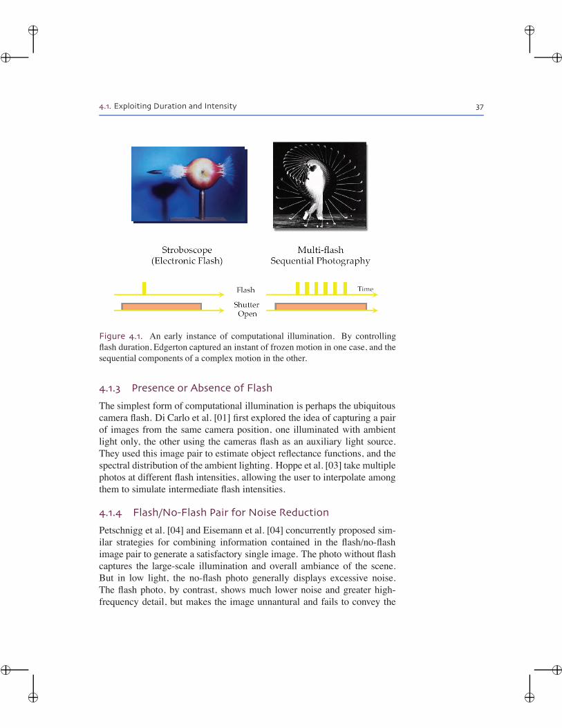
�
�
�
�
�
�
�
�
4.1. Exploiting Duration and Intensity 37
Figure 4.1. An early instance of computational illumination. By controllingflash duration, Edgerton captured an instant of frozen motion in one case, and thesequential components of a complex motion in the other.
4.1.3 Presence or Absence of Flash
The simplest form of computational illumination is perhaps the ubiquitouscamera flash. Di Carlo et al. [01] first explored the idea of capturing a pairof images from the same camera position, one illuminated with ambientlight only, the other using the cameras flash as an auxiliary light source.They used this image pair to estimate object reflectance functions, and thespectral distribution of the ambient lighting. Hoppe et al. [03] take multiplephotos at different flash intensities, allowing the user to interpolate amongthem to simulate intermediate flash intensities.
4.1.4 Flash/No-Flash Pair for Noise Reduction
Petschnigg et al. [04] and Eisemann et al. [04] concurrently proposed sim-ilar strategies for combining information contained in the flash/no-flashimage pair to generate a satisfactory single image. The photo without flashcaptures the large-scale illumination and overall ambiance of the scene.But in low light, the no-flash photo generally displays excessive noise.The flash photo, by contrast, shows much lower noise and greater high-frequency detail, but makes the image unnantural and fails to convey the
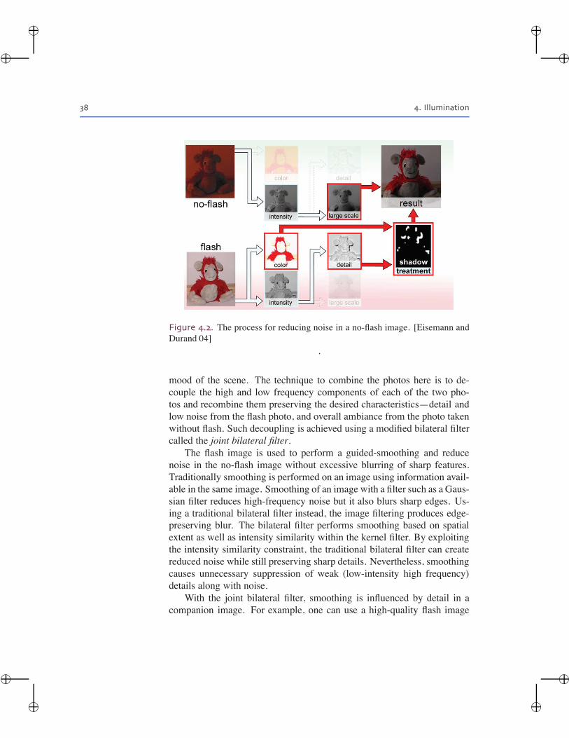
�
�
�
�
�
�
�
�
38 4. Illumination
Figure 4.2. The process for reducing noise in a no-flash image. [Eisemann andDurand 04]
.
mood of the scene. The technique to combine the photos here is to de-couple the high and low frequency components of each of the two pho-tos and recombine them preserving the desired characteristics—detail andlow noise from the flash photo, and overall ambiance from the photo takenwithout flash. Such decoupling is achieved using a modified bilateral filtercalled the joint bilateral filter.
The flash image is used to perform a guided-smoothing and reducenoise in the no-flash image without excessive blurring of sharp features.Traditionally smoothing is performed on an image using information avail-able in the same image. Smoothing of an image with a filter such as a Gaus-sian filter reduces high-frequency noise but it also blurs sharp edges. Us-ing a traditional bilateral filter instead, the image filtering produces edge-preserving blur. The bilateral filter performs smoothing based on spatialextent as well as intensity similarity within the kernel filter. By exploitingthe intensity similarity constraint, the traditional bilateral filter can createreduced noise while still preserving sharp details. Nevertheless, smoothingcauses unnecessary suppression of weak (low-intensity high frequency)details along with noise.
With the joint bilateral filter, smoothing is influenced by detail in acompanion image. For example, one can use a high-quality flash image
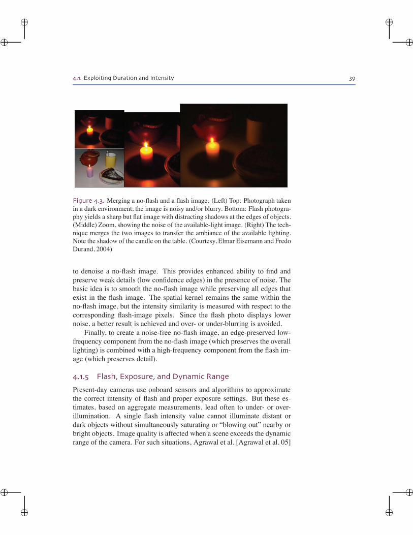
�
�
�
�
�
�
�
�
4.1. Exploiting Duration and Intensity 39
Figure 4.3. Merging a no-flash and a flash image. (Left) Top: Photograph takenin a dark environment; the image is noisy and/or blurry. Bottom: Flash photogra-phy yields a sharp but flat image with distracting shadows at the edges of objects.(Middle) Zoom, showing the noise of the available-light image. (Right) The tech-nique merges the two images to transfer the ambiance of the available lighting.Note the shadow of the candle on the table. (Courtesy, Elmar Eisemann and FredoDurand, 2004)
to denoise a no-flash image. This provides enhanced ability to find andpreserve weak details (low confidence edges) in the presence of noise. Thebasic idea is to smooth the no-flash image while preserving all edges thatexist in the flash image. The spatial kernel remains the same within theno-flash image, but the intensity similarity is measured with respect to thecorresponding flash-image pixels. Since the flash photo displays lowernoise, a better result is achieved and over- or under-blurring is avoided.
Finally, to create a noise-free no-flash image, an edge-preserved low-frequency component from the no-flash image (which preserves the overalllighting) is combined with a high-frequency component from the flash im-age (which preserves detail).
4.1.5 Flash, Exposure, and Dynamic Range
Present-day cameras use onboard sensors and algorithms to approximatethe correct intensity of flash and proper exposure settings. But these es-timates, based on aggregate measurements, lead often to under- or over-illumination. A single flash intensity value cannot illuminate distant ordark objects without simultaneously saturating or “blowing out” nearby orbright objects. Image quality is affected when a scene exceeds the dynamicrange of the camera. For such situations, Agrawal et al. [Agrawal et al. 05]
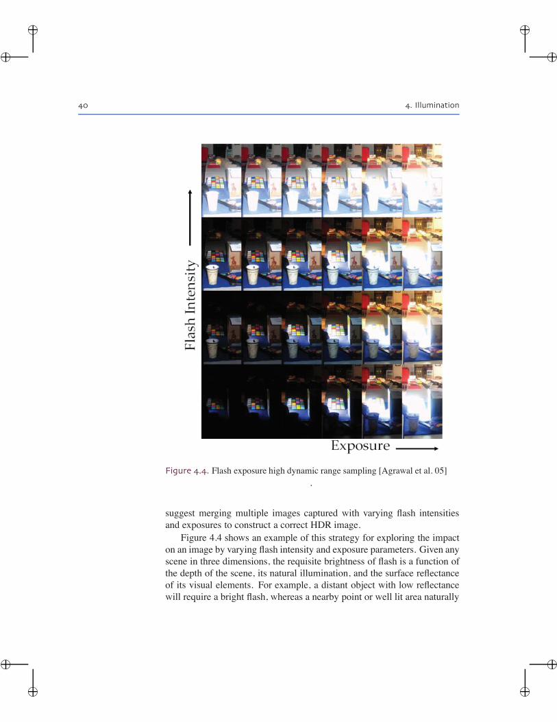
�
�
�
�
�
�
�
�
40 4. Illumination
Figure 4.4. Flash exposure high dynamic range sampling [Agrawal et al. 05].
suggest merging multiple images captured with varying flash intensitiesand exposures to construct a correct HDR image.
Figure 4.4 shows an example of this strategy for exploring the impacton an image by varying flash intensity and exposure parameters. Given anyscene in three dimensions, the requisite brightness of flash is a function ofthe depth of the scene, its natural illumination, and the surface reflectanceof its visual elements. For example, a distant object with low reflectancewill require a bright flash, whereas a nearby point or well lit area naturally
�
�
�
�
�
�
�
�
4.1. Exploiting Duration and Intensity 41
will be over-exposed by a flash, even at lower flash intensity. The scenemight extend to a far off depth that would not be illuminated by even anintensely bright flash; only a longer exposure time would properly captureit. To capture such a challenging scene with a mixed depth, reflectance,and natural lighting, one may need to make multiple exposures, each at adifferent setting along the exposure and flash-intensity axes. The exampleshows photos taken at six different exposure settings, without flash and atthree different flash brightness settings—a total of 24 exposures. Manyconsumer cameras as well as professional cameras offer manual setting offlash intensity. Though making 24 captures to achieve a single image maybe excessive, Agrawal et al. present a greedy approach: pixel values ofeach capture are analyzed for over- or under-exposure, suggesting optimalexposure and flash parameter setting for the subsequent capture [Agrawalet al. 05]. A greedy algorithm makes the locally optimal choice at eachstage in order to calculate the global optimum. By adaptive sampling ofthe flash-exposure space, the number of captured images required for anygiven scene is minimized.
4.1.6 Removing Flash Artifacts
Flash images suffer notoriously from several problems: over-exposure, orblowing-out of nearby objects, poor illumination of distant objects, reflec-tions from objects strongly lit by the flash and strong highlights, reflec-tions of the flash itself, on glossy surfaces. One approach has been themerging of a flash and an ambient image pair to produce better flash im-ages. Agrawal et al. [Agrawal et al. 05] use a technique based on imageintensity gradients. The orientation of the gradient’s vector at a pixel in arasterized image is given by the direction with maximum rate of changeof intensity. The magnitude is the rate of that change. For example, inan intensity edge, the gradient vector orientation is perpendicular to theedge and gradient vector magnitude is the strength of the edge. Agrawal etal. observe that the orientation of image gradients due to reflectance or ge-ometry are illumination-invariant, whereas those due to changes in lightingare not. Hence, the gradient coherence model indicates that in the absenceof artifacts, the gradient vector orientation in flash and ambient (no-flash)images should be the same. On the other hand, a change in gradient vectororientation indicates presence of an artifact. They propose a gradient pro-jection scheme to decompose the illumination effects from the rest of theimage. The gradient projection scheme is based on a gradient coherencemodel.
�
�
�
�
�
�
�
�
42 4. Illumination
Given a set of gradient vectors at each pixel, i.e., a gradient vectorfield, it is possible to reconstruct an image that satisfies the gradient field.Several new techniques have emerged since 2002 based on such gradientvector manipulation and image reconstruction.
Figure 4.5 shows flash and ambient images of a painting. The ambi-ent image includes distracting reflections of the photographer. The low-exposure flash image avoids these reflections, but shows a hot spot. Re-flections in the ambient image are removed by subtracting the componentof the ambient image gradients perpendicular to the flash image gradients.Reconstruction from the projected gradients produces a reflection-free im-age. Reconstruction from residual gradients recovers the reflection layer.However, the gradient orientation in not available when both images haveco-located artifacts (photographer reflection as well as flash hot-spot). Inaddition, gradient orientation is unstable in homogeneous flat regions, sophotographer reflection in such parts will be difficult to recover in suchregions. In later works, Agrawal et al. have introduced a gradation projec-tion tensor which is more robust compared to the simple gradient projec-
Figure 4.5. Removing flash artifacts with gradient vector projection. Undesir-able artifacts in photography can be reduced by comparing image gradients atcorresponding locations in a flash and ambient image pair [Agrawal et al. 05].
�
�
�
�
�
�
�
�
4.2. Modifying Color and Wavelength 43
Figure 4.6. Flash matting allows extraction of foreground using an additionalflash image [Jian et al. 06].
tion procedure. Their work also shows how to compensate for the falloffof flash intensity along the axis of depth of a scene by exploiting the ratioof the flash and ambient photos.
4.1.7 Flash-Based Matting
Matting, to extract a foreground subject from its background, can be mademore precise by combining flash matting with more conventional Bayesianmatting Jian et al. 06]. Inspired by the simple observation that the great-est difference between the flash and the ambient images of such a pair—provided the background is sufficiently distant—is the quality of illumi-nation of the foreground subject, this approach is readily applicable toimages produced by off-the-shelf flash-equipped cameras. For example,a pixel-wise ratio of flash image and no-flash image will be close to 1.0for distant points (background) but significantly higher for nearer points(foreground). With a joint Bayesian matting, even foreground subjectswith complex edges, such as fur or hair, can be more precisely extractedwith an alpha-matt and placed into a new image context. Unlike traditionalBayesian matting, this 2-photo technique works even when foreground andbackground have similar colors. However, the technique fails when theflash image does not encode the distance related fall-off in the expectedway. For example the background is not sufficiently far away, or when theobject is rounded
4.2 Modifying Color and Wavelength
The scene radiance is a product of incident illumination and reflectance.By changing the wavelength profile (often simplified as color profile) of
�
�
�
�
�
�
�
�
44 4. Illumination
the incoming light or capturing specific wavelength channels, one can per-form programmable color manipulations of images.
By changing the spectrum of illumination, it is possible to probe ascene and create multi-spectral photos or overcome confusion due tometamers (colors that have the same visual appearance for a given illu-minant color). Fluorescence photography, commonly used in medical andscientific imaging, exploits the color shift between incident illuminationcolor and the resultant radiance. Many naturally occurring substances flu-oresce, including rocks and minerals, fungi, bacteria, and most body tis-sues. The scene is illuminated with higher frequency (lower wavelength)illumination which results in emission in lower frequency (higher wave-length). Thus, for example, subjects irradiated with ultraviolet may re-lease, green, yellow, or pink light, and subjects irradiated with visible lightmay emit infrared fluorescence. Household fabrics are treated with fluo-rescent dyes to make them look whiter. When illuminated with ultravioletlight (in dimly lit discos, say), the clothes emit several lower frequenciesand appear bright. In most fluorescence photography, a UV wavelengthselective filter is placed at the light source. Another filter of a different(visible) wavelength selection is placed over the camera lens to absorb thereflected ultraviolet rays, permitting only the visible light (fluorescence)from the object itself to be sensed. Fluorescent marker dyes are used to im-age objects inside a scattering medium such as internal biological samplesfeatures in microscopy. By using a wavelength-rejecting optical filter infront of a camera, we can reject all scattered light that has the same wave-length. The induced fluorescence, however, has a different wavelength andcan be imaged by this camera.
Let us look at an example where this wavelength manipulation is donein post-capture stage. Paul Haeberli showed that using multiple exposuresof the same subject with different lighting schemes, allows the lighting ofthe scene to be modified after it has been photographed Haeberli 92]. Heillustrates the technique with a scene lighted with two lamps, to the leftand to the right of the subject (Figure 4.7), in addition to ambient lighting.Three exposures are made, one with ambient lighting only, one with onlythe lamp on the left plus ambient light, and the third with only the lampon the right plus ambient light. The ambient light image is subtractedfrom each of the images lighted by the lamps. “This gives us an imagethat shows exactly what light is contributed by each light source . . . Nowwe can simulate what the scene would look like if the lamp on the leftwas blue instead of white . . . By applying a similar process to the lamp on
�
�
�
�
�
�
�
�
4.3. Position and Orientation of Lighting 45
Figure 4.7. Programmable combination of colors [Haeberli 06].
the right, we can now synthetically illuminate the scene with multicoloredlamps. The brightness and color of any number of lamps can be controlledin this way.” This strategy allows also for negative lighting by subtractinglight coming from a particular lamp.
4.3 Position and Orientation of Lighting
The placement and orientation of auxiliary lighting can also be altered,modifying the shading of subjects as well as shadows throughout an image.Changing the orientation of light with shaped output profile also changesits absolute intensity, but does not change the angle of incidence of lightrays at any point in the scene.
4.3.1 Shape and Detail Enhancement using Multi-PositionFlashes
Amoving light source can be used to inspect and extract subtle surface de-tail and also distinguish silhouettes of objects. A traditional edge-detectionfilter in images can detect the reflectance-discontinuities but does a poorjob in estimating edges due to shape discontinuities. Shape discontinu-ities occur due to depth difference (between a foreground and backgroundpatch) or due to sharp change in surface orientation (a ridge or a valley).By observation under a moving light source, and noting shading and shad-ows, one can highlight such discontinuity.
Raskar et. al. employed a camera equipped with multiple flashesto find the silhouettes in a scene and create stylized or cartoon-like im-ages [Raskar et al. 04]. The multi-flash camera employs four strategicallyplaced flashes to cast shadows along the depth discontinuities of a scene.Depth discontinues are edges in the scene due to shape boundaries or sil-
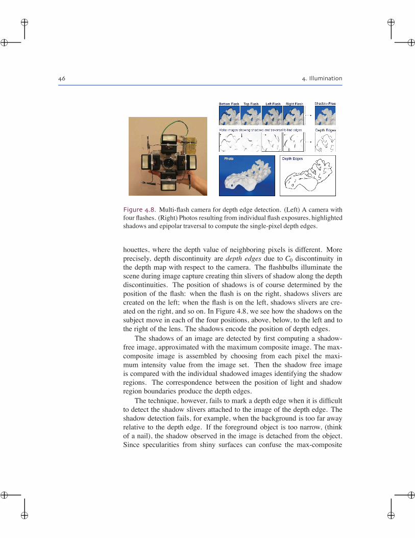
�
�
�
�
�
�
�
�
46 4. Illumination
Figure 4.8. Multi-flash camera for depth edge detection. (Left) A camera withfour flashes. (Right) Photos resulting from individual flash exposures, highlightedshadows and epipolar traversal to compute the single-pixel depth edges.
houettes, where the depth value of neighboring pixels is different. Moreprecisely, depth discontinuity are depth edges due to C0 discontinuity inthe depth map with respect to the camera. The flashbulbs illuminate thescene during image capture creating thin slivers of shadow along the depthdiscontinuities. The position of shadows is of course determined by theposition of the flash: when the flash is on the right, shadows slivers arecreated on the left; when the flash is on the left, shadows slivers are cre-ated on the right, and so on. In Figure 4.8, we see how the shadows on thesubject move in each of the four positions, above, below, to the left and tothe right of the lens. The shadows encode the position of depth edges.
The shadows of an image are detected by first computing a shadow-free image, approximated with the maximum composite image. The max-composite image is assembled by choosing from each pixel the maxi-mum intensity value from the image set. Then the shadow free imageis compared with the individual shadowed images identifying the shadowregions. The correspondence between the position of light and shadowregion boundaries produce the depth edges.
The technique, however, fails to mark a depth edge when it is difficultto detect the shadow slivers attached to the image of the depth edge. Theshadow detection fails, for example, when the background is too far awayrelative to the depth edge. If the foreground object is too narrow, (thinkof a nail), the shadow observed in the image is detached from the object.Since specularities from shiny surfaces can confuse the max-composite
�
�
�
�
�
�
�
�
4.3. Position and Orientation of Lighting 47
image, the authors described a method using an intrinsic image (describedin Section 4.5 instead of the max-image. The detected silhouettes are thenused to stylize the photograph and highlight important features. Raskar etal. demonstrated similar silhouette detection in video using a high-speedflash sequence [Raskar et al. 04].
Using a larger number of images captured with varying light positionsaround the photographic subject in a studio (or laboratory) setting, one canenhance the subtle surface features as observed in grazing angle illumi-nation, shadows due to complex geometry, specularities, and subsurfacescattering.
Akers et al. [Akers et al. 03] use spatially varying image weights onimages acquired with a light stage similar to the work of Debevec [De-bevec et al. 01]. A painting interface allows the artist to locally modify arelit image as desired. Although the spatially varying mask offers greaterflexibility, it can also produce physically unrealizable results that appearunrealistic. Anrys et al. [Anrys et al. 04] and Mohan et al. [Mohan etal. 05] used a similar painting interface to help a novice in photographiclighting design. A target image is sketched, and the system is allowed tofind optimal weights for each input image in order to achieve a physicallyrealizable result closest to the target.
4.3.2 Relighting Using Domes and Light Waving
The goal of image-based relighting is to create arbitrary novel lighting ina photo in post-capture editing. Instead of building an accurate 3D modelof the scene appearance, image-based relighting relies on the simple ob-servation that light interacts linearly with material objects [Nimeroff, 94,Haeberli 92]. If the scene is lit by one light, then doubling the pixel inten-sities in a photo will achieve the same effect as doubling the brightness ofthe light source. This of course assumes that the camera response is linear,without underexposure or saturation. Adding two photos, each taken withonly one light, is equivalent to capturing a photo with two lights. Moreprecisely, if a fixed camera makes an image Ii from a fixed scene lit onlyby a light Li, then the same scene lit by many lights scaled by weightswi will produce an image Iout = ∑i(wiIi). Adjusting weights allows us tocreate an output image from a linear combination of input images. How-ever, due to linearity, the effective output image is the same as if the lightsources had been modulated (turned brighter or dimmer). This achievesdigital post-capture relighting of the image.
�
�
�
�
�
�
�
�
48 4. Illumination
For accurate relighting of a scene to synthesize arbitrary virtual light-ing conditions, ideally we need to photograph the scene by moving thelight through every possible position of the lighting fixture—a challeng-ing task. For example, let us say that we limit light positions within asquare on a flat surface and take successive photos by moving the lightsource within that square. From this dataset, we can resynthesize photosonly from virtual light sources lying within that square. To overcome thislimitation and reduce the number of lighting variations required, we canexploit the fact that all incident light can be geometrically parameterizedby a 5D plenoptic function, i.e., 5D ray-representation. Effectively, weneed to make an exposure by turning on lighting just one ray at a time. Ifwe limit ourselves to resynthesizing novel lights positioned only outsidethe convex hull of the object, however, the problem is slightly simplified.In this case, we can represent the incident light field (illumination field) us-ing a 4D ray parameterization. To understand this, we need to consider thehigher-dimensional incident light field (illumination field) and its impacton the resultant outgoing light field.
We discussed light fields earlier in Chapter 2. Light fields and lumi-graphs reduced the more general 5D plenoptic function to a four-dimensional function, L(u,v,s, t) that describes the presence of light infree space, ignoring the effects of wavelength and time [Adelson 91]. Here(u,v) and (s, t), respectively, are the parameters on two parallel planes thatdescribe a ray of light in space. To represent the illumination field on anobject, a slightly different parameterization can be used.
Imagine the object surrounded by a spherical dome with projectorsaimed inwards. Parameter (θi,φi) describes the angular position of theprojector on the unit sphere, and (u,v) the pixel position in the projectedimage from that projector. Thus, the function Li(u,v,θ ,φ) gives completecontrol over the incident light rays on an object in free space. Similarly,an array of cameras on that spherical dome aimed inwards would capturethe entire radiant light field of an object, Lr(u,v,θ ,φ). Debevec et al. in-troduced the 8D reflectance field that describes the relationship of the 4Dincident light fileds plus the 4D radiant light fields of a scene [Debevec etal. 01]. An additional dimension of time is sometimes added to describethe changing interaction of light with an object over time.
For relighting, we are interested in a fixed viewpoint; hence from a 4Dradiant field, we capture only a 2D photo. Along with the 4D incident illu-mination field, this becomes a problem of 6D reflectance-field estimation.While the reflectance field gives a complete description of the interaction
�
�
�
�
�
�
�
�
4.3. Position and Orientation of Lighting 49
of light with a scene, its acquisition would require photographing the sceneby turning on one ray at a time. This will require inordinate quantities oftime and storage. Significant strides have been made toward acquiringlower-dimensional subsets of this function and using it for restricted re-lighting and rendering.
Debevec et. al. employed a light stage comprising a light mounted ona rotating robotic arm to acquire the non-local reflectance field of a humanface [Debevec et al. 01]. The point-like light source can be thought of asa simplified projector of a single pixel. Thus, the incident light field is re-duced to a 2D function. The reflectance field with a 2D incident light fieldplus a 2D photos is therefore only 4D. The generation of novel images un-der arbitrary lighting was demonstrated. This was accomplished simply byadjusting the weights wi to match the desired intensity of illumination fromvarious directions. Going beyond relighting, the authors added a smallnumber of cameras all firing in parallel to capture images of the face fromneighboring viewpoints. They were able to simulate small alterations ofviewpoint using a simple model for skin reflectance. Hawkins et al. em-ployed a similar configuration to digitize cultural artifacts by capturingreflectance fields. They argue for the use of the reflectance field in digitalarchiving, rather than geometric models and reflectance textures [Hawkinset al. 01]. Koudelka, et. al. captured a set of images from a single view-point as a point light source rotated around the photographic subject andestimated the surface geometry by using two sets of basis images. Fromtheir estimation of the apparent BRDF for each pixel in the images, theycould render the subject under arbitrary illumination [Koudelka et al. 01].
Debevec et al. proposed an enhanced light stage comprising a largenumber (156) of inwardly oriented LEDs distributed over a spherical struc-ture approximately two meters in diameter around the photographic sub-jectin this instance, an actor (Figure 4.9 (left)). Each light was set to anarbitrary color and intensity to simulate the effect of a real-world environ-ment around the actor (Figure 4.9 (center)). The images gathered fromthe light stage, together with a mask of the actor captured with infra-red sources and detector, were used to composite the actor seamlesslyinto a virtual set, while maintaining consistent illumination (Figure 4.9(right)) [Debevec et al. 02]. Malzbender et al. employed 50 inwardly ori-ented flashes distributed over a hemispherical dome, together with a novelscheme for compressing and storing the 4D reflectance field called thepolynomial texture map [Malzbender et al. 01]. They assumed that thecolor of a pixel changed smoothly as the light moved around the object
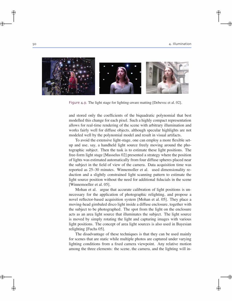
�
�
�
�
�
�
�
�
50 4. Illumination
Figure 4.9. The light stage for lighting-aware matting [Debevec et al. 02].
and stored only the coefficients of the biquadratic polynomial that bestmodelled this change for each pixel. Such a highly compact representationallows for real-time rendering of the scene with arbitrary illumination andworks fairly well for diffuse objects, although specular highlights are notmodeled well by the polynomial model and result in visual artifacts.
To avoid the extensive light-stage, one can employ a more flexible set-up and use, say, a handheld light source freely moving around the pho-tographic subject. Then the task is to estimate these light positions. Thefree-form light stage [Masselus 02] presented a strategy where the positionof lights was estimated automatically from four diffuse spheres placed nearthe subject in the field of view of the camera. Data acquisition time wasreported as 25–30 minutes. Winnemoller et al. used dimensionality re-duction and a slightly constrained light scanning pattern to estimate thelight source position without the need for additional fiducials in the scene[Winnemoeller et al. 05].
Mohan et al. argue that accurate calibration of light positions is un-necessary for the application of photographic relighting, and propose anovel reflector-based acquisition system [Mohan et al. 05]. They place amoving-head gimbaled disco light inside a diffuse enclosure, together withthe subject to be photographed. The spot from the light on the enclosureacts as an area light source that illuminates the subject. The light sourceis moved by simply rotating the light and capturing images with variouslight positions. The concept of area light sources is also used in Bayesianrelighting [Fuchs 05].
The disadvantage of these techniques is that they can be used mainlyfor scenes that are static while multiple photos are captured under varyinglighting conditions from a fixed camera viewpoint. Any relative motionamong the three elements: the scene, the camera, and the lighting will in-
�
�
�
�
�
�
�
�
4.3. Position and Orientation of Lighting 51
troduce artifacts. Some of these problems can be addressed using motioncompensation via image registration. But often the motion of any one ofthe elements creates two different relative motions. This makes it quitechallenging to use these methods for traditional photography. Neverthe-less, in many controllable setting these methods can be used.
4.3.3 Towards Reflectance Fields Capture in 4D, 6D, and 8D
Themost complete image-based description of a scene for computer graph-ics applications is its 8D reflectance field [Debevec et al. 00]. Themeasure-ment of reflectance fields is an active area of research. The 8D reflectancefield is a transport that describes the transfer of energy between a light fieldof incoming rays (the illumination) and a light field of outgoing rays (theview) in a scene, each of which is 4D. As we saw earlier this represen-tation can be used to synthesize images of the scene from any viewpointunder arbitrary lighting. Note that the synthesized results demonstrate allglobal illumination effects such as diffuse inter-reflections, shadows, caus-tics and sub-surface scattering, without the need for an explicit physicalsimulation.
However, most of this research has focused on capturing meaningfullower-dimensional slices of the 8D reflectance field. Earlier, we saw ex-amples of capturing 4D datasets for relighting from a fixed viewpoint andvariable lighting. If the illumination is provided by an array of video pro-jectors and the scene is captured as illuminated by each pixel of each pro-jector, but still as seen from a single viewpoint, then one obtains a 6Dslice of an 8D reflectance field. If we use k projectors each with a millionpixels, we need to capture k-million photos for this 6D dataset since wecan measure the impact of only projector pixels in each photo. Masseluset al. captured such data sets using a single moving projector positionedin the k positions [Masselus et al. 03]. Sen et al. exploited Helmholtzreciprocity to develop a dual photography approach [Sen et al. 05]. TheHelmholtz reciprocity allows you to interchange the projectors and cam-eras in a scene. Instead of one camera and k projectors, they used k cam-eras and one projector. Unlike an array of (lights or) projectors, an ar-ray of cameras can operate in parallel without interference. By turningon each projector pixel, one for each photo, but simultaneously capturingk photos, the authors improved on the capture times of these data sets.An earlier method for capturing the full 8D reflectance field exploited thedata-sparseness of the 8D transport matrix to represent the transport ma-trix by local rank-1 approximations. Based on the sparsity observations,
�
�
�
�
�
�
�
�
52 4. Illumination
the authors developed a hierarchical parallelized acquisition technique thatsignificantly sped up the reflectance field capture process [Garg et al. 06].
4.4 Modulation in Space and Time
The capacity to modulate the intensity of flash over space and time pro-vides additional control of the resulting image. An intelligent flash wouldbehave much like a projector. A projector allows modulation of ray in-tensities in each ray direction by changing pixel intensities and is an easilyavailable programmable spatio-temporally modulated light-emitter. Henceprojectors are commonly used in computational illumination research, al-though they are inconvenient for incorporation in a practical camera. Usinga projector-like light source as a camera flash, which allows us to changenot only the overall brightness but also rapidly change the radiance of ev-ery ray emitted from the projector-flash, is a powerful alternative to con-ventional flash, as it provides full control over the 2D set of rays it emitsvia pixel intensity manipulation. Shree Nayar coined the term “CamPro”to designate a projector that is supporting the operation of a camera [Na-yar 06]. A projector can project arbitrarily complex illumination patternsonto the scene, capture the corresponding images, and compute informa-tion regarding the scene that is impossible to obtain with traditional flash.Captured images are optically coded by the patterned illumination of thescene. In the future, then, the unwieldy projector may be replaced by smartlasers or light sources with highly programmable mask patterns.
4.4.1 Projector for Structured Light
For scanning the 3D surface of opaque objects, coded structured light isconsidered one of the most reliable techniques. This technique is based onprojecting a light pattern and imaging the illuminated scene from one ormore cameras to simplify the well known correspondence problem. Givena pair of images of the same 3D scene, captured from two different pointsof view, the correspondence problem is to find a set of points in one imageidentical to points in another image. For an arbitrary 3D point, its repre-sentation in the two images generates the pair of corresponding pixels. Inturn, given the pair of corresponding pixels in two images, by triangulatonone can compute the 3D location of that point. In the case of projectedstructured light, a single camera view can be used along with the projectorview. The projected pattern is coded so that over time each projector pixel
�
�
�
�
�
�
�
�
4.4. Modulation in Space and Time 53
is assigned a unique binary. Thanks to this coding, correspondences be-tween camera image points and points of the projector pattern can easilybe decoded. By triangulating the decoded points, 3D information is recov-ered. In place of a passive camera, the projector actively encodes the spacevia illumination. Hence this is known as active stereo triangulation. For agood overview, see [Salvi et al. 02]. Coding schemes continue to evolve.The number of projected patterns required to encode the projector pixelcan be reduced by exploiting color. Rusinkiewicz et al. exploited modestassumptions about local smoothness of surface and reflectance and deriveda new set of illumination patterns based on coding the boundaries betweenprojected stripes Rusinkiewicz et al. 02].
4.4.2 High Spatial Frequency Patterns
Active illumination approaches have been used to analyze multi-path lightscattering, and to compute the inverse of the light transport. Consider ascene lit by a point light source and viewed by a camera. The brightnessof each scene point has two components: direct and global. The directcomponent results from light received directly from the source. The globalcomponent results from light received from all other points in the scene.It turns out that individual materials exhibit unique and fascinating directand global illumination properties. A traditional camera receives a sum ofthe two. But a programmable flash can be used to separate a scene into itsdirect and global components. The two components can then be used toedit the physical properties of objects in the scene to produce novel images.The image on the left side of Figure 4.10 shows a scene captured using acheckerboard illumination pattern. If the checkerboard patterns frequencyis high, then the camera brightness of a point lit by one of the white squaresincludes the direct component and exactly half of the global componentbecause the checkerboard pattern lights only half of the remaining scenepoints.
Now consider a second image captured using the complement of thisillumination pattern. In this case, the point does not have a direct com-ponent but still produces exactly half of the global component. This isbecause the complementary checkerboard pattern lights the remaining halfof scene points. Since the above argument applies to all points in the scene,the direct and global components of all the scene points can be measuredby projecting just two illumination patterns. The middle of Figure 4.10shows separation results for a scene with peppers of different colors. Thedirect image includes mainly the specular reflections from the surfaces of
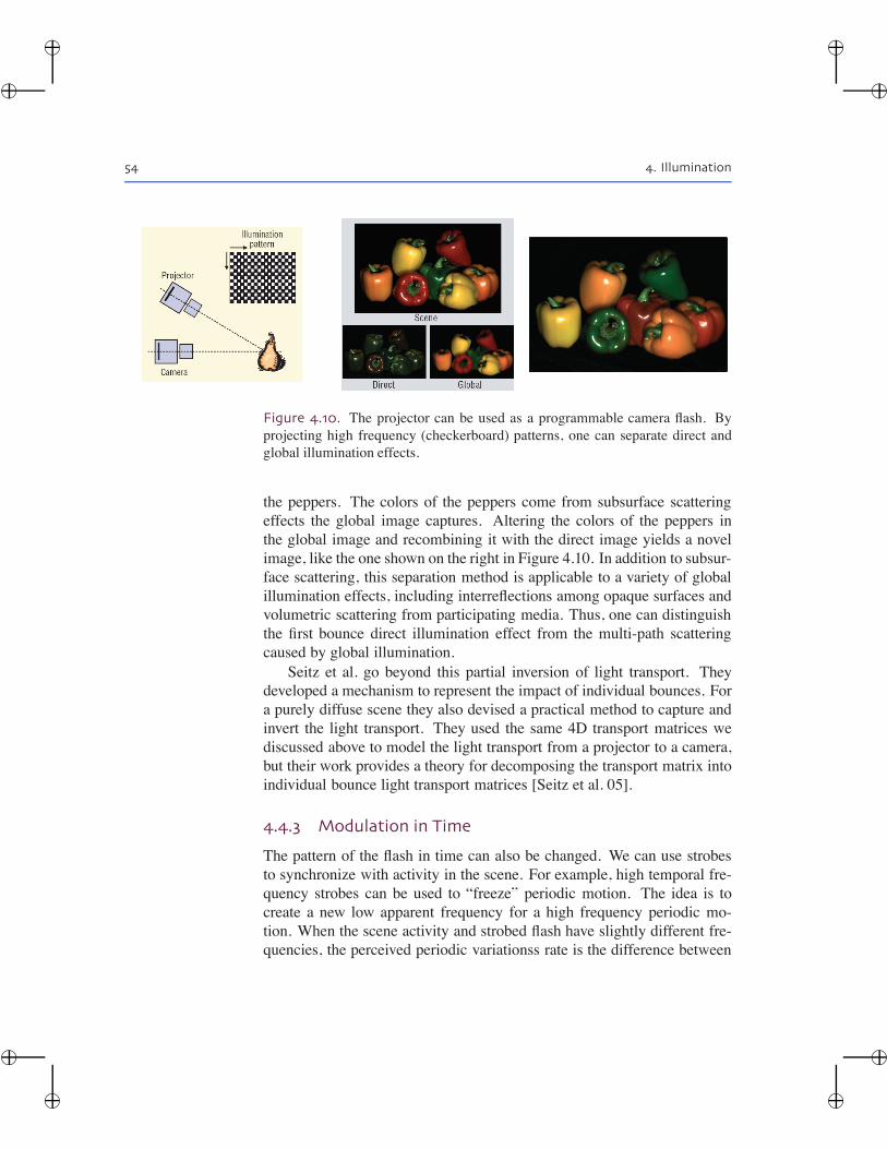
�
�
�
�
�
�
�
�
54 4. Illumination
Figure 4.10. The projector can be used as a programmable camera flash. Byprojecting high frequency (checkerboard) patterns, one can separate direct andglobal illumination effects.
the peppers. The colors of the peppers come from subsurface scatteringeffects the global image captures. Altering the colors of the peppers inthe global image and recombining it with the direct image yields a novelimage, like the one shown on the right in Figure 4.10. In addition to subsur-face scattering, this separation method is applicable to a variety of globalillumination effects, including interreflections among opaque surfaces andvolumetric scattering from participating media. Thus, one can distinguishthe first bounce direct illumination effect from the multi-path scatteringcaused by global illumination.
Seitz et al. go beyond this partial inversion of light transport. Theydeveloped a mechanism to represent the impact of individual bounces. Fora purely diffuse scene they also devised a practical method to capture andinvert the light transport. They used the same 4D transport matrices wediscussed above to model the light transport from a projector to a camera,but their work provides a theory for decomposing the transport matrix intoindividual bounce light transport matrices [Seitz et al. 05].
4.4.3 Modulation in Time
The pattern of the flash in time can also be changed. We can use strobesto synchronize with activity in the scene. For example, high temporal fre-quency strobes can be used to “freeze” periodic motion. The idea is tocreate a new low apparent frequency for a high frequency periodic mo-tion. When the scene activity and strobed flash have slightly different fre-quencies, the perceived periodic variationss rate is the difference between
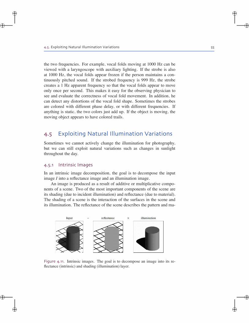
�
�
�
�
�
�
�
�
4.5. Exploiting Natural Illumination Variations 55
the two frequencies. For example, vocal folds moving at 1000 Hz can beviewed with a laryngoscope with auxiliary lighting. If the strobe is alsoat 1000 Hz, the vocal folds appear frozen if the person maintains a con-tinuously pitched sound. If the strobed frequency is 999 Hz, the strobecreates a 1 Hz apparent frequency so that the vocal folds appear to moveonly once per second. This makes it easy for the observing physician tosee and evaluate the correctness of vocal fold movement. In addition, hecan detect any distortions of the vocal fold shape. Sometimes the strobesare colored with different phase delay, or with different frequencies. Ifanything is static, the two colors just add up. If the object is moving, themoving object appears to have colored trails.
4.5 Exploiting Natural Illumination Variations
Sometimes we cannot actively change the illumination for photography,but we can still exploit natural variations such as changes in sunlightthroughout the day.
4.5.1 Intrinsic Images
In an intrinsic image decomposition, the goal is to decompose the inputimage I into a reflectance image and an illumination image.
An image is produced as a result of additive or multiplicative compo-nents of a scene. Two of the most important components of the scene areits shading (due to incident illumination) and reflectance (due to material).The shading of a scene is the interaction of the surfaces in the scene andits illumination. The reflectance of the scene describes the pattern and ma-
Figure 4.11. Intrinsic images. The goal is to decompose an image into its re-flectance (intrinsic) and shading (illumination) layer.
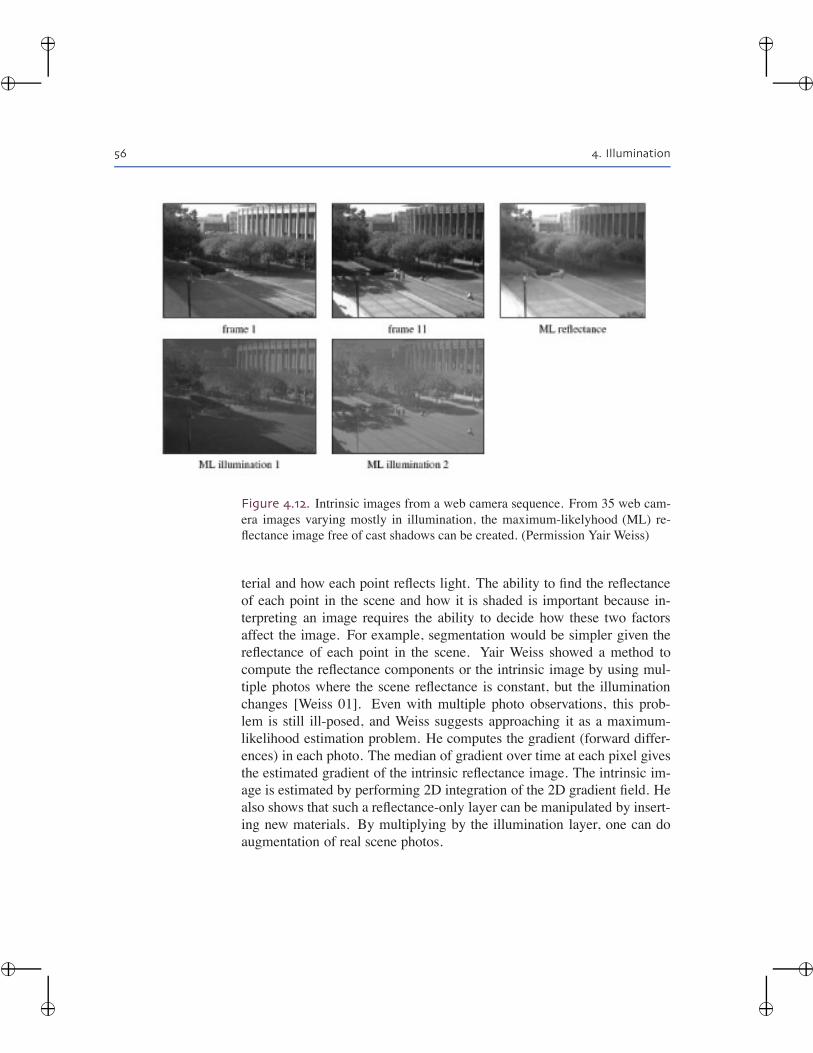
�
�
�
�
�
�
�
�
56 4. Illumination
Figure 4.12. Intrinsic images from a web camera sequence. From 35 web cam-era images varying mostly in illumination, the maximum-likelyhood (ML) re-flectance image free of cast shadows can be created. (Permission Yair Weiss)
terial and how each point reflects light. The ability to find the reflectanceof each point in the scene and how it is shaded is important because in-terpreting an image requires the ability to decide how these two factorsaffect the image. For example, segmentation would be simpler given thereflectance of each point in the scene. Yair Weiss showed a method tocompute the reflectance components or the intrinsic image by using mul-tiple photos where the scene reflectance is constant, but the illuminationchanges [Weiss 01]. Even with multiple photo observations, this prob-lem is still ill-posed, and Weiss suggests approaching it as a maximum-likelihood estimation problem. He computes the gradient (forward differ-ences) in each photo. The median of gradient over time at each pixel givesthe estimated gradient of the intrinsic reflectance image. The intrinsic im-age is estimated by performing 2D integration of the 2D gradient field. Healso shows that such a reflectance-only layer can be manipulated by insert-ing new materials. By multiplying by the illumination layer, one can doaugmentation of real scene photos.
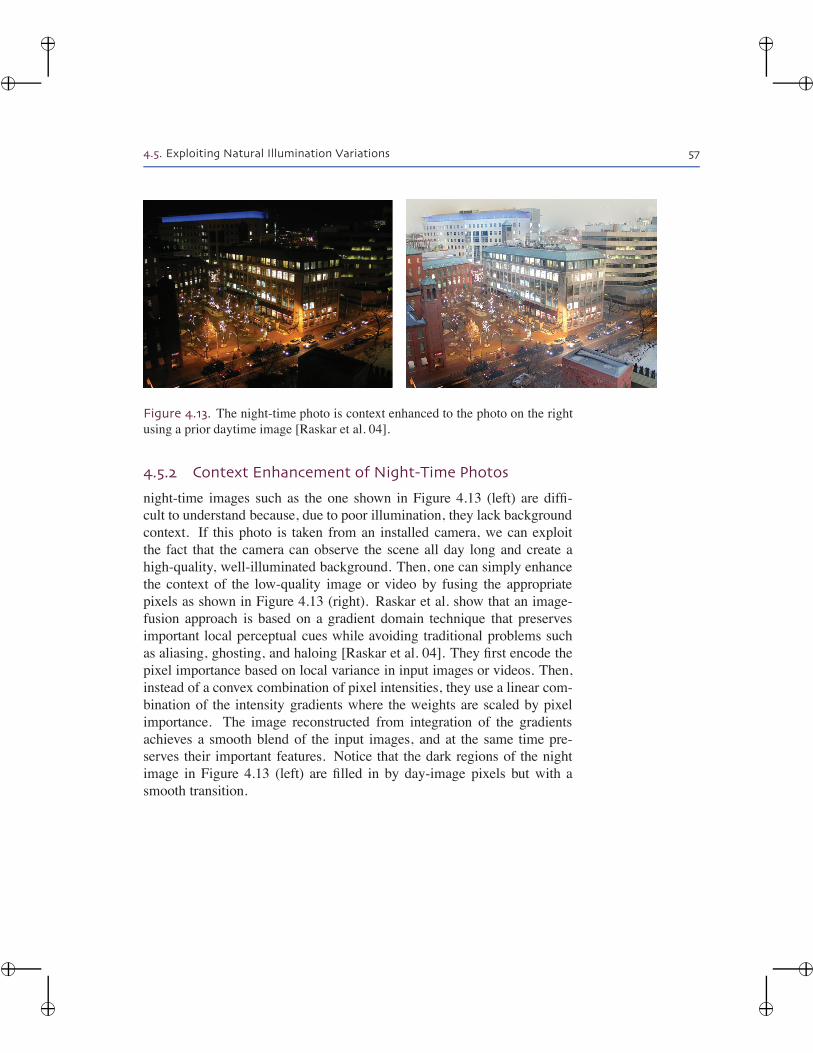
�
�
�
�
�
�
�
�
4.5. Exploiting Natural Illumination Variations 57
Figure 4.13. The night-time photo is context enhanced to the photo on the rightusing a prior daytime image [Raskar et al. 04].
4.5.2 Context Enhancement of Night-Time Photos
night-time images such as the one shown in Figure 4.13 (left) are diffi-cult to understand because, due to poor illumination, they lack backgroundcontext. If this photo is taken from an installed camera, we can exploitthe fact that the camera can observe the scene all day long and create ahigh-quality, well-illuminated background. Then, one can simply enhancethe context of the low-quality image or video by fusing the appropriatepixels as shown in Figure 4.13 (right). Raskar et al. show that an image-fusion approach is based on a gradient domain technique that preservesimportant local perceptual cues while avoiding traditional problems suchas aliasing, ghosting, and haloing [Raskar et al. 04]. They first encode thepixel importance based on local variance in input images or videos. Then,instead of a convex combination of pixel intensities, they use a linear com-bination of the intensity gradients where the weights are scaled by pixelimportance. The image reconstructed from integration of the gradientsachieves a smooth blend of the input images, and at the same time pre-serves their important features. Notice that the dark regions of the nightimage in Figure 4.13 (left) are filled in by day-image pixels but with asmooth transition.

�
�
�
�
�
�
�
�
�
�
�
�
�
�
�
�
Bibliography
Fusion of Images Taken by Varying Cameraand Scene Parameters
General
[Akers et al. 03] David Akers, Frank Losasso, Jeff Klingner, Maneesh Agrawala,John Rick, and Pat Hanrahan. “Conveying Shape and Features with Image-Based Relighting.” In Proceedings of the 14th IEEE Visualization 2003(VIS’03), pp. 349–354. Washington, DC: IEEE Computer Society, 2003.
[Burt and Kolczynski 93] P. Burt and R. Kolczynski. “Enhanced Image Capturethrough Fusion.” In Proceedings of the Fourth International Conference onComputer Vision, pp. 173–182. Los Alamos, CA: IEEE Press, 1993.
[Levin et al. 04] A. Levin, A. Zomet, S. Peleg, and Y. Weiss. “Seamless ImageStitching in the Gradient Domain.” InComputer Vision-ECCV 04: 8th Euro-pean Conference on Computer Vision, Prague, Czech Republic, May 11–14,2004, Proceedings, Lecture Notes in Computer Science 3024, pp. 377–389.Berlin: Springer, 2004.
[Massey and Bender 96] M. Massey and W. Bender. “Salient Stills: Process andPractice.” IBM Systems Journal 35:3&4 (1996), 557–574.
[Mutter and Krause 92] S. Mutter and M. Krause. Surrational Images: Pho-tomontages. Champaign, IL: University of Illinois Press, 1992.
[Robinson 69] H. P. Robinson. Pictorial Effect in Photography: Being Hints onComposition and Chiaroscuro for Photographers. London: Piper & Carter.1869.
[Muybridge 55] E. Muybridge. The Human Figure in Motion. New York: DoverPublications, Inc., 1955.
59
�
�
�
�
�
�
�
�
60 Bibliography
[Agarwala et al. 04] A. Agarwala, M. Dontcheva, M. Agrawala, S. Drucker, A.Colburn, B. Curless, D. Salesin and M. Cohen. “Interactive Digital Pho-tomontage.” In ACM SIGGRAPH 2004 Papers, pp. 294–302. New York:ACM Press, 2004.
[Nayar and Narasimhan 02] S. K. Nayar and S. G. Narasimhan. ““Assorted Pix-els: Multi-Sampled Imaging with Structural Models.” In Computer Vision-ECCV 2002: 7th European Conference on Computer Vision, Copenhagen,Denmark, May 28-31, 2002. Proceedings, Part IV, Lecture Notes in Com-puter Science 2353, pp. 636–652. Berlin: Springer, 2002.
Time
[Braun 92] M. Braun. Picturing Time: The Work of Etienne-Jules Marey.Chicago: The University of Chicago Press, 1992.
[Freeman and Zhang 03] W. T. Freeman and H. Zhang. “Shape-Time Photogra-phy.” In Proceedings of the 2003 IEEE Computer Society Conference onComputer Vision and Pattern Recognition, pp. 151–157. Los Alamitos, CA:IEEE Press, 2003.
Exposure
[Fattal et al. 02] R. Fattal, D. Lischinski and M. Werman. “Gradient DomainHigh Dynamic Range Compression.” ACM Transactions on Graphics 21:3(2002), 249–256.
[Reinhard et al. 02] E. Reinhard, M. Stark, P. Shirley, and J. Ferwerda. “Pho-tographic Tone Reproduction for Digital Images.” ACM Transactions onGraphics 21:3 (2002), 267-276.
[Debevec and Malik 97] P. E. Debevec and J. Malik. “Recovering High DynamicRange Radiance Maps from Photographs.” In Proceedings of SIGGRAPH97, Computer Graphics Proceedings, Annual Conference Series, edited byTurner Whitted, pp. 369-378. Reading, MA: Addison-Wesley, 1997.
[Durand and Dorsey 02] F. Durand and J. Dorsey. “Fast Bilateral Filtering for theDisplay of High-Dynamic-Range Images.” ACM Transactions on Graphics21:3 (2002), 257-266.
[Mann and Picard 95] S. Mann and R. W. Picard. “Being ’Undigital’ with DigitalCameras: Extending Dynamic Range by Combining Differently ExposedPictures.” In Proceedings of the 47th Annular Conference of the Society forImaging Science and Technology, pp. XX-XX. Springfield, VA: The Societyof Imaging Science and Technology, 1995.
�
�
�
�
�
�
�
�
Bibliography 61
[Tumblin and Turk 99] Jack Tumblin and Greg Turk. “LCIS: A Boundary Hi-erarchy for Detail-Preserving Contrast Reduction.” In Proceedings of SIG-GRAPH 99, Computer Graphics Proceedings, Annual Conference Series,edited by Alyn Rockwood, pp. 83-90. Reading, MA: AddisonWesley Long-man, 1999.
[DiCarlo and Wandell 00] J. DiCarlo and B. Wandell. “Rendering High DynamicRange Images.” In Sensors and Camera Systems for Scientific, Industrial,and Digital Photography Applications (Proceedings Volume), Proceedingsof SPIE 3965, pp. 392-401. Bellingham, WA: SPIE, 2000.
[Kang et al. 03] S. B. Kang, M. Uyttendaele, S. Winder, and R. Szeliski. “HighDynamic Range Video.” ACM Transactions on Graphics 22:3 (2003), 319-325.
Focus
[Haeberli 94] P. Haeberli. Grafica Obscura: Collected Computer GraphicsHacks. Available at http://www.sgi.com/grafica/, 1994
[McGuire et al. 05] Morgan McGuire, Wojciech Matusik, Hanspeter Pfister,John F. Hughes, and Fredo Durand. “Defocus Video Matting.” Proceedingsof ACM SIGGRAPH 2005: ACM Transactions on Graphics 24:3 (2005),567-576.
Illumination
[Anrys and Dutre 04] Frederik Philip. “Image Based Lighting Design.” In Pro-ceedings of the Fourth IASTED International Conference on Visualization,Imaging, and Image Processing, edited by Juan J. Villanieva, pp. 222- 230.Calgary: ACTA Press, 2004.
[Akers et al. 03] David Akers, Frank Losasso, Jeff Klingner, Maneesh Agrawala,John Rick, and Pat Hanrahan. “Conveying Shape and Features with Image-Based Relighting.” In Proceedings of the 14th IEEE Visualization 2003(VIS’03), pp. 349-354. Washington, DC: IEEE Computer Society, 2003.
[Agrawa et al. 05] Amit Agrawal, Ramesh Raskar, Shree K. Nayar, andYuanzhen Li. “Removing Photography Artifacts Using Gradient Projectionand Flash-Exposure Sampling.” In Proceedings of ACM SIGGRAPH 2005:ACM Transactions on Graphics 24:3 (2005), 828-835.
[Debeve et al. 00] Paul Debevec, Tim Hawkins, Chris Tchou, Haarm-PieterDuiker, Westley Sarokin, and Mark Sagar. “Acquiring the Reflectance Field
�
�
�
�
�
�
�
�
62 Bibliography
of a Human Face.” In Proceedings of SIGGRAPH 2000, Computer Graph-ics Proceedings, Annual Conference Series, edited by Kurt Akeley, pp. 145-156. Reading, MA: Addison- Wesley, 2000.
[Debevec et al. 02] Paul Debevec, AndreasWenger, Chris Tchou, Andrew Gard-ner, JamieWaese, and Tim Hawkins. “A Lighting Reproduction Approachto Live-Action Compositing.” In Proceedings of ACM SIGGRAPH 2002:ACM Transactions on Graphics 21:3 (2002), 547-556.
Passive Illumination
[Raskar et al. 04] R. Raskar, A. Ilie, and J. Yu. “Image Fusion for Context En-hancement and Video Surrealism.” In Proceedings of the 3rd InternationalSymposium on Non-photorealistic Animation and Rendering, pp. 85-152.New York: ACM Press, 2004.
[Weiss 01] Y. Weiss. “Deriving Intrinsic Images from Image Sequences.” In Pro-ceedings of the Eighth IEEE International Conference on Computer Vision(ICCV 2001), pp. 68-75. Los Alamitos, CA: IEEE Press, 2001.
Polarization
[Schechner et al. 01] Y. Y. Schechner, S. G. Narasimhan, and S. K. Nayar. “In-stant Dehazing of Images Using Polarization.” In Proceedings of IEEE Con-ference on Computer Vision and Pattern Recognition, Vol. I, pp. 325- 332.Los Alamitos, CA: IEEE Press, 2001.
[Nayar et al. 93] S. K. Nayar, X. Fang, and T. E. Boult. “Removal of Speculari-ties Using Color and Polarization.” In Proceedings of IEEE Computer Soci-ety Conference on Computer Vision and Pattern Recognition, pp. 583-590.Los Alamitos, Ca: IEEE Computer Society, 1993.
[Wu and Walsh 03] P. Wu and J. T. Walsh. “Tissue Polarization Imaging ofMultiply-Scattered Reflected Light Lasers.” in Lasers in Surgery andMedicine 23, Supplement 15 (2003), XX-XX.
Wavelength
[Socolinsky 00] D. A. Socolinsky. “Dynamic Range Constraints in Image Fusionand Realization.” Proc. IASTED Int. Conf. Signal and Image Process, 349-354 (2000).
[Schechner and Nayar 04] Y. Y. Schechner and S. K. Nayar. “UncontrolledMod-ulation Imaging.” In Proceedings of the 2004 IEEE Computer Society Con-ference on Computer Vision and Pattern Recognition, Vol. 2, pp. 197-204.Los Alamitos, CA: IEEE Computer Society, 2004.
�
�
�
�
�
�
�
�
Bibliography 63
Location
[Agarwala et al. 06] Aseem Agarwala, Maneesh Agrawala, Michael Cohen,David Salesin, and Rick Szeliski. “Photographing Long Scenes with Multi-Viewpoint Panoramas.” Proceedings of SIGGRAPH 2006: ACM Transac-tions on Graphics 25:3 (2006), 853-861.
[Wilburn et al. 05] B. Wilburn, N. Joshi, V. Vaish, E. Talvala, E. Antunez, A.Barth, A. Adams, M. Horowitz, and M. Levoy. “High-Performance Imag-ing Using Large Camera Arrays.” Proceedings of ACM SIGGRAPH 2005:ACM Transactions on Graphics 24:3 (2005), 765-776.
[Snavely et al. 06] Noah Snavely, Steven M. Seitz, and Richard Szeliski. “PhotoTourism: Exploring Photo Collections in 3D.” In ACM SIGGRAPH 2006Papers, pp. 835-846. New York: ACM Press, 2006.
[Rother et al. 06] Carsten Rother, Lucas Bordeaux, Youssef Hamadi, and An-drewBlake. “AutoCollage.” In ACMSIGGRAPH 2006 Papers, pp. 847-852.New York: ACM Press, 2006.
Matting
[Chuang et al. 01] Y.-Y. Chuang, B. Curless, D. Salesin, and R. Szeliski. “ABayesian Approach to Digital Matting.” In Proceedings of the 2001 IEEEComputer Society Conference on Computer Vision and Pattern Recognition,Vol. II, pp. 264-271. Los Alamitos, CA: IEEE Computer Society, 2001.
[Porter and Duff 84] T. Porter and T. Duff. “Compositing Digital Images.” InProceedings of ACM SIGGRAPH 84: Computer Graphics 18 (1984), 253-259.
[Smith and Blinn 96] A. R. Smith and J. F. Blinn. “Blue screen Matting.” In Pro-ceedings of SIGGRAPH 96, Computer Graphics Proceedings, Annual Con-ference Series, edited by Holly Rushmeier, pp. 259-268. Reading, MA: Ad-dison Wesley, 1996.
[Sun et al. 04] Jian Sun, Jiaya Jia, Chi-Keung Tang, and Heung-Yeung Shum.“Poisson Matting.” Proceedings of SIGGRAPH 2004: ACM Transactionson Graphics 23:3 (2004), 315-321.
Image Manipulation
[Jia et al. 06] Jiaya Jia, Jian Sun, Chi-Keung Tang, and Heung-Yeung Shum.“Drag-and-Drop Pasting.” In ACM SIGGRAPH 2006 Papers, pp. 631-637.New York: ACM Press, 2006.
�
�
�
�
�
�
�
�
64 Bibliography
[Bae et al. 06] Soonmin Bae, Sylvain Paris, and Fredo Durand. “Two-Scale ToneManagement for Photographic Look.” In ACM SIGGRAPH 2006 Papers,pp. 637-645. New York: ACM Press, 2006.
[Lischinski et al. 06] Dani Lischinski, Zeev Farbman, Matt Uyttendaele, andRichard Szeliski. “Interactive Local Adjustment of Tonal Values.” In ACMSIGGRAPH 2006 Papers, pp. 646-653. New York: ACM Press, 2006.
[Khan et al. 06] Erum Arif Khan, Erik Reinhard, Roland W. Fleming, and Hein-rich H. Bulthoff. “Image-Based Material Editing.” In ACM SIGGRAPH2006 Papers, pp. 654-663. New York: ACM Press, 2006.
[Oliva et al. 06] Aude Oliva, Antonio Torralba, and Philippe G. Schyns. “HybridImages.” In ACM SIGGRAPH 2006 Papers, pp. 527-532. New York: ACMPress, 2006.
Techniques
General
[Danielsson 80] P.-E. Danielsson. “Euclidean Distance Mapping.” ComputerGraphics and Image Processing 14 (1980), 227-248.
[Lucas and Kanade 81] B. D. Lucas and T. Kanade. “An Iterative Image Regis-tration Technique with an Application to Stereo Vision. In Proceedings ofthe 7th International Joint Conference on Artificial Intelligence (IJCAI ’81),pp. 674-679. San Francisco: Morgan Kaufmann, 1981.
[Mortensen and Barrett 95] E. N. Mortensen andW. A. Barrett. “Intelligent Scis-sors for Image Composition.” In Proceedings of SIGGRAPH 95, ComputerGraphics Proceedings, Annual Conference Series, edited by Robert Cook,pp. 191-198. Reading, MA: Addison Wesley, 1995.
Graph Cuts
[Boykov et al. 01] Y. Boykov, O. Veksler, and R. Zabih. “Fast Approximate En-ergy Minimization via Graph Cuts.” IEEE Transactions on Pattern Analysisand Machine Intelligence 23:11 (2001), 1222-1239.
[Kwatra et al. 03] V. Kwatra, A. Schodl, I. Essa, G. Turk, and A. Bobick. “Graph-cut Textures: Image and Video Synthesis Using Graph Cuts.” ACM Trans-actions on Graphics 22:3 (2003), 277-286.
�
�
�
�
�
�
�
�
Bibliography 65
[Shi and Malik 97] J. Shi and J. Malik. “Normalized Cuts and Image Segmen-tation.” In Proceedings of the 1997 IEEE Computer Society Conference onComputer Vision and Pattern Recognition, pp. 731-737. Los Alamitos, CA:IEEE Computer Society, 1997.
Gradient Domain
[Perez et al. 03] P. Perez, M. Gangnet, and A. Blake. “Poisson Image Editing.”ACM Transactions on Graphics 22:3 (2003), 313-318.
[Georgiev 06] T. Georgiev. “Covariant Derivatives and Vision.” In ComputerVision-ECCV 2006: 9th European Conference on Computer Vision, Graz,Austria, May 7-13, 2006, Proceedings, Part IV, Lecture Notes in ComputerScience 3954, pp.56-69. Berlin: Springer, 2006.
Smoothing, Bilateral, and Trilateral Filters
[Tomasi and Manduchi 98] C. Tomasi and R. Manduchi. “Bilateral Filtering ofGray and Colored Images.” In Proceedings of the Sixth IEEE InternationalConference on Computer Vision, pp. 836-846. Los Alamitos, CA: IEEEComputer Society, 1998.
[Choudhury and Tumblin 03] P. Choudhury and J. Tumblin. “The Trilateral Fil-ter for High Contrast Images and Meshes.” In Proceedings of the 14th Euro-graphics Workshop on Rendering, edited by Per. H. Christensen and DanielCohen, pp. 186-196. Aire-la-Ville, Switzerland: Eurographics Association,2003.
Video Textures
[Schodl et al. 00] A. Schodl, R. Szeliski, D. H. Salesin, and I. Essa. “Video Tex-tures.” In Proceedings of the 27th Annual Conference on Computer Graphicsand Interactive Techniques, pp. 489-498. New York: ACM Press/Addison-Wesley Publishing Co., 2000.
[Agarwala et al. 05] A. Agarwala, K. C. Zheng, C. Pal, M. Agrawala, M. Cohen,B. Curless, D. Salesin, and R. Szeliski. “Panoramic Video Textures.” ACMTransaction on Graphics 24:3 (2005), 821-827.
�
�
�
�
�
�
�
�
66 Bibliography
Feature Extraction and Scene Understanding
Shape/Material/Illumination and Surface Normals
[Basri and Jacobs 01] R. Basri and D. Jacobs. “Photometric Stereo with General,Unknown Lighting.” In Proceedings of the 2001 IEEE Computer SocietyConference on Computer Vision and Pattern Recognition, Vol. II, pp. 374-381. Los Alamitos, CA: IEEE Computer Society, 2001.
[Horn 70] B. K. P. Horn. “Shape from Shading: A Method for Obtaining theShape of a Smooth Opaque Object from One View.” MIT Project MAC In-ternal Report TR-79 and MIT AI Lab Technical Report 232, 1970.
[Zickler et al. 02] Todd Zickler, Peter N. Belhumeur, and David J. Kriegman,“Helmholtz Stereopsis: Exploiting Reciprocity for Surface Reconstruction.”In Computer Vision-ECCV 2002: 7th European Conference on ComputerVision, Copenhagen, Denmark, May 28-31, 2002, Proceedings, Part III,Lecture Notes in Computer Science 2352, Part III, pp 869-884. Berlin,Springer, 2002.
[Wenger et al. 05] AndreasWenger, AndrewGardner, Chris Tchou, Jonas Unger,Tim Hawkins, and Paul. Debevec. “Performance Relighting and ReflectanceTransformation with Time-Multiplexed Illumination.” In ACM SIGGRAPH2005 Papers, pp. 756-764. New York: ACM Press, 2005.
Depth Edges
[Raskar et al. 04] Ramesh Raskar, Karhan Tan, Rogerio Feris, Jingyi Yu, andMatthew Turk. “Non-photorealistic Camera: Depth Edge Detection andStylized Rendering Using Multi-flash Imaging.” In ACM SIGGRAPH 2004Papers, pp. 679-688. New York, ACM Press, 2004.
Depth
[Nayar and Nakagawa 94] S. K. Nayar and Y. Nakagawa. “Shape from Focus.”IEEE Transactions on Pattern Analysis and Machine Intelligence 16:8(1994), 824-831.
Motion
[Ben-Ezra and Nayar 04] M. Ben-Ezra and S. K. Nayar, “Motion-Based MotionDeblurring.” IEEE Transactions on Pattern Analysis and Machine Intelli-gence 26:6 (2004), 689-698.
�
�
�
�
�
�
�
�
Bibliography 67
[Raskar et al. 06] R. Raskar, A. Agrawal, and J. Tumblin. “Coded Exposure Pho-tography: Motion Deblurring Using Fluttered Shutter.” ACM Transactionson Graphics 25:3 (2006), 795-804.
[Fergus et al. 06] Rob Fergus, Barun Singh, Aaron Hertzmann, Sam T. Roweis,and William T. Freeman. “Removing Camera Shake from a Single Pho-tograph.” Proceedings of ACM SIGGRAPH 2006: ACM Transactions onGraphics 25:3 (2006), 787-794.
[Liu et al. 05] C. Liu, A. Torralba, W. T. Freeman, F. Durand, and E. H. Adelson.“Motion Magnification.” ACM Transactions on Graphics 24:3 (2005), 519-526.
Decomposition of Scene Parameters
[Nayar et al. 06] Shree K. Nayar, Gurunandan Krishnan, Michael D. Grossberg,and Ramesh Raskar. “Fast Separation of Direct and Global Components ofa Scene Using High Frequency Illumination.” In ACM SIGGRAPH 2006Papers, pp. 935-944. New York: ACM Press, 2006.
Transfer and Denoising
Flash to No-Flash
[Eisemann and Durand 04] Elmar Eisemann and Fredo Durand. “Flash Photog-raphy Enhancement via Intrinsic Relighting.” In ACM SIGGRAPH 2004Papers, pp. 673-678. New York: ACM Press, 2004.
[Petschnigg et al. 04] Georg Petschnigg, Richard Szeliski, Maneesh Agrawala,Michael Cohen, Hugues Hoppe, and Kentaro Toyama. “Digital Photographywith Flash and No-Flash Image Pairs.” Proceedings of SIGGRAPH 2004:ACM Transactions on Graphics 23:3 (2004), 664-672.
[DiCarlo et al. 01] J. M. DiCarlo, F. Xiao, and B. A. Wandell. “Illuminating Il-lumination.” In Proceedings of the Ninth Color Imaging Conference, pp.27-34. Springfield, VA: The Society of Imaging Science and Technology,2001.
Noise
[Meer et al. 90] P. Meer, J. Jolion, and A. Rosenfeld. “A Fast Parallel Algo-rithm for Blind Estimation of Noise Variance.” IEEE Transactions on PatternAnalysis and Machine Intelligence, 12:2 (1990), 216-223.
�
�
�
�
�
�
�
�
68 Bibliography
[Bennett and McMillan 05] Eric P. Bennett and Leonard McMillan. “Video En-hancement Using Per-Pixel Virtual Exposures.” In ACM SIGGRAPH 2005Papers, pp. 845-852. New York: ACM Press, 2005.
Geometric Operations
Panorama
[Davis 98] J. Davis. “Mosaics of Scenes with Moving Objects.” In Proceedingsof the 1998 Conference on Computer Vision and Pattern Recognition, pp.354-360. Los Alamitos, CA: IEEE Computer Society, 1998.
[Uyttendaele et al. 01] M. Uyttendaele, A. Eden, and R. Szeliski. “EliminatingGhosting and Exposure Artifacts in Image Mosaics.” In Proceedings of the2001 Conference on Computer Vision and Pattern Recognition, Vol. II, pp.509-516. Los Alamitos, CA: IEEE Computer Society, 2001.
[Szeliski and Shum 97] R. Szeliski and H.-Y. Shum. “Creating Full ViewPanoramicMosaics and EnvironmentMaps.” In Proceedings of SIGGRAPH97, Computer Graphics Proceedings, Annual Conference Series, edited byTurner Whitted, pp. 251-258. Reading, MA: Addison Wesley, 1997.
Synthetic Aperture and Multi-views
[Adelson and Wang 92] E. H. Adelson and J. Y.A. Wang. “Single Lens Stereowith a Plenoptic Camera.” IEEE Transactions on Pattern Analysis and Ma-chine Intelligence 14:2 (1992), 99-106.
[Levoy and Hanrahan 96] Marc Levoy and Pat Hanrahan. “Light Field Render-ing.” In Proceedings of SIGGRAPH 96, Computer Graphics Proceedings,Annual Conference Series, edited by Holly Rushmeier, pp. 31-42. Reading,MA: Addison Wesley, 1996.
[Gortler et al. 96] Steven J. Gortler, Radek Grzeszczuk, Richard Szeliski, andMichael F. Cohen. “The Lumigraph.” In Proceedings of SIGGRAPH 96,Computer Graphics Proceedings, Annual Conference Series, edited byHolly Rushmeier, pp. 43-54. Reading, MA: Addison Wesley, 1996.
[Levoy et al. 06] Marc Levoy, Ren Ng, Andrew Adams, Matthew Footer, andMark Horowitz. “Light Field Microscopy.” In ACM SIGGRAPH 2006 Pa-pers, pp.924-934. New York: ACM Press, 2006.
[Levoy et al. 04] Marc Levoy, Billy Chen, Vaibhav Vaish, Mark Horowitz, IanMcDowall, and Mark Bolas. “Synthetic Aperture Confocal Imaging.” InACM SIGGRAPH 2004 Papers, pp. 825-834. New York: ACM Press, 2004.
�
�
�
�
�
�
�
�
Bibliography 69
[Hg 05] Ren Ng. “Fourier Slice Photography.” In ACM SIGGRAPH 2005 Pa-pers, pp. 735-744. New York: ACM Press, 2005.
[Georgiev et al. 06] Todor Georgiev, Ke Colin Zheng, Brian Curless, DavidSalasin, Shree Nayar, and Chintan Intwala. “Spatio-Angular ResolutionTradeoff in Integral Photography.” In Rendering Techniques 2006: Euro-graphics Symposium on Rendering, edited by T. Akenine-Moller and W.Heidrich, pp. 263-272. Aire-la-Ville, Switzerland: Eurographics Associa-tion, 2006.
[Stern and Javidi 03] A. Stern and B. Javidi. “3-D Computational SyntheticAperture Integral Imaging (COMPSAII).” Optics Express 11 (2003), 2446-2451.
[Oliver and Quegan 98] C. Oliver and S. Quegan.Understanding Synthetic Aper-ture Radar Images. London: Artech House, 1998.
[Vaish et al. 05] Vaibhav Vaish, Gaurav Garg, Eino-Ville Talvala, Emilio An-tunez, Bennett Wilburn, Mark Horowitz, and Marc Levoy. “Synthetic Aper-ture Focusing Using a Shear-Warp Factorization of the Viewing Transform.”In Proceedings of the 2005 IEEE Computer Society Conference on Com-puter Vision and Pattern Recongnition, Vol. 3, pp. 129. Los Alamitos, CA:IEEE Computer Society, 2005.
[Joshi et al. 06] Neel Joshi, Wojciech Matusik, and Shai Avidan. “Natural VideoMatting Using Camera Arrays.” In ACM SIGGRAPH 2006 Papers, pp. 779-786. New York: ACM Press, 2006.
[Kuthirummal and Nayar 06] Sujit Kuthirummal and Shree K. Nayar. “Multi-view Radial Catadioptric Imaging for Scene Capture.” In ACM SIGGRAPH2006 Papers, pp. 916-923. New York: ACM Press, 2006.
Deblurring and Superresolution
[Ben-Ezra and Nayar 03] M. Ben-Ezra and S. K. Nayar. “Motion Deblurring Us-ing Hybrid Imaging.” In Proceedings of the 2003 IEEE Computer SocietyConference on Computer Vision and Pattern Recognition, Vol. I, pp. 657-664. Los Alamitos, CA: IEEE Computer Society, 2003.
[Lin and Shum 04] Zhouchen Lin and Heung-Yeung Shum. “Fundamental Lim-its of Reconstruction-Based Superresolution Algorithms under Local Trans-lation.” IEEE Transactions on Pattern Analysis and Machine Intelligence26:1 (2004), 83-89.
[Landolt et al. 01] O. Landolt, A. Mitros, and C. Koch. “Visual Sensor withResolution Enhancement by Mechanical Vibrations.” In Proceedings of the
�
�
�
�
�
�
�
�
70 Bibliography
2001 Conference on Advanced Research in VLSI, pp. 249-264. Los Alami-tos, CA: IEEE Computer Society, 2001.
[Zhang and Nayar 06] Li Zhang and Shree Nayar. “Projection Defocus Analysisfor Scene Capture and Image Display.” In ACM SIGGRAPH 2006 Papers,pp. 907-915. New York: ACM Press, 2006.
Dynamic Range
[Morimura 93] A. Morimura. “Imaging Method for a Wide Dynamic Range andan Imaging Device for a Wide Dynamic Range.” U.S. Patent no. 5,455,621,1993.
[Burt and Kolczynski 93] P. Burt and R. J. Kolczynski. “Enhanced Image Cap-ture Through Fusion.” In Proceedings of the Fourth International Confer-ence on Computer Vision, pp. 173-182, 1993. Los Alamitos, CA: IEEEPress, 1993.
[Madden 93] B. Madden. “Extended Intensity Range Imaging.” Technical ReportMS-CIS-93-96, Grasp Laboratory, University of Pennsylvania, 1993.
[Tsai 94] Y. T. Tsai. “Method and Apparatus for Extending the Dynamic Rangeof an Electronic Imaging System.” U.S. Patent no. 5,309,243, 1994.
[Mitsunaga and Nayar 99] T. Mitsunaga and S. K. Nayar. “Radiometric Self Cal-ibration.” In Proceedings of the 1999 IEEEComputer Society Conference onComputer Vision and Pattern Recognition, Vol. 2, pp. 374-380. Los Alami-tos, CA: IEEE Computer Society, 1999.
[Street 98] R. A. Street. “High Dynamic Range Segmented Pixel Sensor Array.”U.S. Patent no. 5,789,737, 1998.
[Handy 86] R. J. Handy. “High Dynamic Range CCD Detector Imager.” U.S.Patent no. 4,623,928, 1986.
[Wen 89] D. D. Wen. “High Dynamic Range Charge Coupled Device.” U.S.Patent no. 4,873,561, 1989.
[Hamazaki 96] M. Hamazaki. “Driving Method for Solid-State Image PickupDevice.” Japanese Patent no. 08- 331461, 1996.
[Knight 83] T. Knight. “Design of an Integrated Optical Sensor with On-ChipPre-processing.” Ph.D. diss., Massachusetts Institute of Technology, 1983.
[Sayag 91] M. Sayag, “Non-linear Photosite Response in CCD Imagers.” U.SPatent no. 5,055,667, 1991.

�
�
�
�
�
�
�
�
Bibliography 71
[Decker et al. 98] S. J. Decker, R. D. McGrath, K. Brehmer, and C. G. Sodini,“A 256 ? 256 CMOS Imaging Array with Wide Dynamic Range Pixels andColumn-Parallel Digital Output.” IEEE Journal of Solid-State Circuits 33(1998), 2081-2091.
[Brajovic and Kanade 96] V. Brajovic and T. Kanade. “A Sorting Image Sensor:An Example of Massively Parallel Intensity-to-Time Processing for Low-Latency Computational Sensors.” In Proceedings of the 1996 IEEE Interna-tional Conference on Robotics and Automation, Vol. 2, pp. 1638-1643. LosAlamitos, CA: IEEE Press, 1996.
[Scheffer et al. 00] D. Scheffer S. Kavadias, B. Dierickx, A. Alaerts, D. Uwaerts,and J. Bogaerts. “A Logarithmic Response CMOS Image Sensor with On-Chip Calibration.” IEEE Journal of Solid-State Circuits 35:8 (2000), 1146-1152.
[Shree and Mitsunaga 00] Shree K. Nayar and Tomoo Mitsunaga. “High Dy-namic Range Imaging: Spatially Varying Pixel Exposures.” In Proceedingsof the IEEE Conference on Computer Vision and Pattern Recognition, pp.1472-1479. Los Alamitos, CA: IEEE Press, 2000:
Active Illumination
[Adelson and Bergen 91] Edward H. Adelson and James R. Bergen. “ThePlenoptic Function and the Elements of Early Vision.” In ComputationalModels of Visual Processing, edited by M. Landy and J. A. Movshon, pp.3-20. Cambridge, MA: MIT Press, 1991.
[Fuchs et al. 05] Martin Fuchs, Volker Blanz, and Hans-Peter Seidel. “BayesianRelighting.” In Proceedings of the Eurographics Symposium on RenderingTechniques, pp. 157-164. Aire-la-Ville, Switzerland: Eurographics Associ-ation 2005.
[Haeberli 08] Paul Haeberli. Graphics Obscura. Available at http://www.graficaobscura.com/, 2008.
[Hawkins et al. 01] Tim Hawkins, Jonathan Cohen, and Paul Debevec. “A Pho-tometric Approach to Digitizing Cultural Artifacts.” In Proceedings of the2001 Conference on Virtual Reality, Archeology, and Cultural Heritage, pp.333-342. New York: ACM Press, 2001.
[Hawkins et al. 05] Tim Hawkins, Per Einarsson, and Paul E. Debevec. “A DualLight Stage.” In Proceedings of the Eurographics Symposium on RenderingTechniques, pp. 91-98. Aire-la-Ville, Switzerland: Eurographics Associa-tion, 2005.
�
�
�
�
�
�
�
�
72 Bibliography
[Hoppe and Toyama 03] Hugues Hoppe and Kentaro Toyama. “ContinuousFlash.” Technical Report 63, Microsoft Research, 2003.
[Jones et al. 05] Andrew Jones, Andrew Gardner, Mark Bolas, Ian McDowall,and Paul Debevec. “Performance Geometry Capture for Spatially VaryingRelighting.” In ACM SIGGRAPH 2005 Sketches, Article no. 74. New York:ACM Press, 2005.
[Xiao et al. 01] Feng Xiao, JeffreyM. DiCarlo, and Brian AWandell. “Illuminat-ing Illumination.” In The 9th Color Imaging Conference, pp. 27-34. Spring-field, VA: The Society for Imaging Science and Technology, 2001.
[Koudelka et al. 01] Melissa L Koudelka, Peter N Belhumeur, Sebastian Magda,and David J. Kriegman. “Image- BasedModeling and Rendering of Surfaceswith Arbitrary BRDFs.” In Proceedings of the 2001 IEEE Computer SocietyConference on Computer Vision and Pattern Recognition, Vol. I, pp. 568-575. Los Alamitos, CA: IEEE Computer Society, 2001.
[Malzbender et al. 01] Tom Malzbender, Dan Gelb, and Hans Wolters. “Polyno-mial TextureMaps.” In Proceedings of SIGGRAPH 2001, Computer Graph-ics Proceedings, Annual Conference Series, edited by E. Fiume, pp. 519-528. New York: ACM Press, 2001.
[Masselus 03] Vincent Masselus, Pieter Peers, Philip Dutre, and Yves D.Willems. “Relighting with 4D Incident Light Fields.” In SIGGRAPH 2003:ACM Transactions on Graphics 22:3 (2003), 613-620.
[Mohan et al. 05] Ankit Mohan, Jack Tumblin, Bobby Bodenheimer, CindyGrimm, and Reynold J. Bailey. “Table- Top Computed Lighting for Prac-tical Digital Photography.” In Proceedings of the Eurographics Symposiumon Rendering Techniques, pp. 165-172. Aire-la-Ville, Switzerland: Euro-graphics Association, 2005.
[Nimeroff et al. 94] Jeffry S. Nimeroff, Eero Simoncelli, and Julie Dorsey. “Effi-cient Re-rendering of Naturally Illuminated Environments.” In Proceedingsof the Fifth Eurographics Workshop on Rendering, pp. 359-373. Aire- la-Ville, Switzerland: Eurographics Association, 1994.
[Wenger et al. 05] AndreasWenger, AndrewGardner, Chris Tchou, Jonas Unger,Tim Hawkins, and Paul Debevec. “Performance Relighting and ReflectanceTransformation with Time-Multiplexed Illumination.” In ACM SIGGRAPH2005 Papers, pp. 756-764. New York: ACM Press, 2005.
[Winnemoeller et al. 05] Holger Winnemoeller, Ankit Mohan, Jack Tumblin,and Bruce Gooch. “Light Waving: Estimating Light Positions from Pho-tographs Alone.” Computer Graphics Forum 24:3 (2005), 433-438.
�
�
�
�
�
�
�
�
Bibliography 73
[Sun et al. 06] Jian Sun, Yin Li, Sing Bing Kang, and Heung-Yeung Shum.“Flash Matting.” In ACM SIGGRAPH 2006 Papers, pp. 772-778. NewYork: ACM Press, 2006.
Smart, Unconventional Cameras
MEMS Technology
[Nayar et al. 04] S. K. Nayar, V. Branzoi, and T. Boult. “Programmable ImagingUsing a Digital Micromirror Array.” In Proceedings of 2004 IEEE ComputerSociety Conference on Computer Vision and Pattern Recognition, Vol. I, pp.436-443. Los Alamitos, CA: IEEE Computer Society, 2004.
High Speed Imaging
[Wandell et al. 99] B. Wandell, P. Catrysse, J. DiCarlo, D. Yang, and A. ElGamal. “Multiple Capture Single Image Architecture with a CMOS Sen-sor.” In Proceedings of the International Symposium onMultispectral Imag-ing and Color Reproduction for Digital Archives, pp. 11-17. Chiba, Japan:Society of Multispectral Imaging of Japan, 1999.
[Kleinfelder et al. 01] S. Kleinfelder, S. H. Lim, X. Q. Liu, and A. El Gamal. “A10,000 Frames/s CMOS Digital Pixel Sensor.” IEEE Journal of Solid-StateCircuits 36:12 (2001), 2049-2059.
[Liu and Gamal 03] X. Q. Liu and Abbas El Gamal. “Synthesis of High DynamicRangeMotion Blur Free Image fromMultiple Captures.” IEEE Transactionson Circuits and Systems 50:4 (2003), 530-539.
[Raskar et al. 06] Ramesh Raskar, Amit AGrawal, and Jack Tumblin. “CodedExposure Photography: Motion Deblurring Using Fluttered Shutter.” InACM SIGGRAPH 2006 Papers, pp. 795-804. New York: ACM Press, 2006.
[Shechtman et al. 02] E. Shechtman, Y. Caspi, and M. Irani. “Increasing Space-Time Resolution in Video.” In Computer Vision-ECCV 2002: 7th EuropeanConference on Computer Vision, Copenhagen, Denmark, May 28-31, 2002,Proceedings, Part I, Lecture Notes in Computer Science 2350, pp. 753-768.Berlin: Springer-Verlag, 2002.
[Johansson et al. 03] R. Johansson, L. Lindgren, J. Melander, and B. Moller. “AMulti-resolution 100-GOPS 4-Gpixels/s Programmable CMOS Image Sen-sor for Machine Vision.” Paper presented at the 2003 IEEE Workshop onCharge-Coupled Devices and Advanced Image Sensors, 2003.
�
�
�
�
�
�
�
�
74 Bibliography
Advanced, Programmable, Demodulating Cameras, andTemporal Correlation
[Xiao et al. 01] F. Xiao, J. DiCarlo, P. Catrysse and B. Wandell, Image Analy-sis using Modulated Light Sources, In Proceedings of the SPIE ElectronicImaging ’2001 conference, Vol. 4306, San Jose, CA, January 2001.
[Ando et al. 97] Ando, S., K. Nakamura, and T. Sakaguchi. Ultrafast CorrelationImage Sensor: Concept, Design, and Applications,. in Proc. IEEE CCD/AISWorkshop. 1997. Bruges, Belgium: IEEE.
[Ando and Kimachi 99] Ando, S. and A. Kimachi. Time-Domain CorrelationImage Sensor: First CMOS Realization of Demodulator Pixels Array. inProc. ’99 IEEE CCD/AIS Workshop. 1999.
Others
[Cohen 05] Michael Cohen. “Capturing the Moment”, Symposium on Computa-tional Photography and Video, Boston in May, 2005.
[Tumblin et al. 05] TUMBLIN, J., AGRAWAL, A. AND RASKAR, R. Why Iwant a Gradient Camera, IEEE CVPR 2005
Optics
[Stam 99] Jos Stam, “Diffraction Shaders”, In SIGGRAPH 99 Conference Pro-ceedings, Annual Conference Series, August 1999, 101-110.
[Elber 94] Elber, G. 1994. Low cost illumination computation using an approx-imation of light wavefronts. In Proceedings of the 21st Annual Conferenceon Computer Graphics and interactive Techniques SIGGRAPH ’94. ACMPress, New York, NY, 335-342.
[Rosenfeld and Kak 87] Rosenfeld A. and Kak A.C., Digital Image Processing,New York; Academic Press, Cap 11, 1987.
[Goodman 68] J.W. Goodman, Introduction to Fourier Optics, McGraw-HillBook Co.,New York, N.Y., (1968).
[Dowski and Cathey 95] Dowski, E.R.,Jr., Cathey, W.T., Extended depth of fieldthrough wave-front coding, Applied Optics, Vol. 34, No. 11, 10 April 1995,pp. 1859-1866.
[Zomet and Nayar 06] A. Zomet and S.K. Nayar, “Lensless Imaging with aControllable Aperture,” IEEE Conference on Computer Vision and PatternRecognition (CVPR), Jun, 2006.
�
�
�
�
�
�
�
�
Bibliography 75
[Zand 96] Zand, J., Coded aperture imaging in high energy astronomy, NASALaboratory for High Energy Astrophysics (LHEA) at NASA’s GSFC, 1996.
Light Field Optics
[Hecht and Zajac 79] E. Hecht and A. Zajac. Optics. Addison-Wesley, 1979.
[Gerrard and Burch 94] A. Gerrard and J. M. Burch. Introduction to MatrixMethods in Optics. Dover Publications, 1994.
[Guillemin and Sternberg] V. Guillemin and S. Sternberg. Symplectic techniquesin physics. Cambridge University Press.
[Durand et al. 05] Fredo Durand, Nicolas Holzschuch, Cyril Soler, Eric Chan &Francois Sillion. A Frequency analysis of Light Transport. Proceedings ofSIGGRAPH 2005.
[Georgiev and Intwala 06] Todor Georgiev, Chintan Intwala. Integral View Pho-tography. Adobe Tech Report 2006:
[Georgiev et al. 06] Todor Georgiev, Colin Zheng, Shree Nayar, DavidSalesin, Brian Curless, Chintan Intwala. Spatio-angular ResolutionTrade-Offs in Integral Photography. In proceedings, EGSR 2006.http://www.tgeorgiev.net/Spatioangular.pdf
Fourier Optics
[Goodman 68] J. Goodman, Introduction to Fourier Optics, McGraw-Hill, 1968.
[Born 64] M. Born, E. Wolf, Principles of Optics, Pergamon Press, 1964.