Computer Architecture- 1 Ping-Liang Lai ( 賴秉樑 ) Chapter 1 Fundamentals of Computer Design Computer Architecture 計算機結構

Computer Architecture- 1

Ping-Liang Lai (賴秉樑 )

Chapter 1Fundamentals of Computer

Design

Computer Architecture計算機結構


Outline

1.1 Introduction 1.2 Classes of Computers 1.3 Defining Computer Architecture 1.4 Trends in Technology 1.5 Trends in Power in Integrated Circuits 1.6 Trends in Cost 1.7 Dependability 1.8 Measuring, Reporting, and Summarizing Performance 1.9 Quantitative Principles of Computer Design 1.10 Putting It All Together: Performance and Price-

Performance


1.1 Introduction

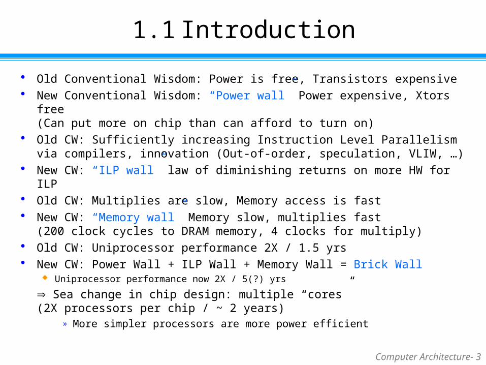
Old Conventional Wisdom: Power is free, Transistors expensive New Conventional Wisdom: “Power wall” Power expensive, Xtors free

(Can put more on chip than can afford to turn on) Old CW: Sufficiently increasing Instruction Level Parallelism via compilers,

innovation (Out-of-order, speculation, VLIW, …) New CW: “ILP wall” law of diminishing returns on more HW for ILP Old CW: Multiplies are slow, Memory access is fast New CW: “Memory wall” Memory slow, multiplies fast

(200 clock cycles to DRAM memory, 4 clocks for multiply) Old CW: Uniprocessor performance 2X / 1.5 yrs New CW: Power Wall + ILP Wall + Memory Wall = Brick Wall

Uniprocessor performance now 2X / 5(?) yrs

Sea change in chip design: multiple “cores” (2X processors per chip / ~ 2 years)

» More simpler processors are more power efficient


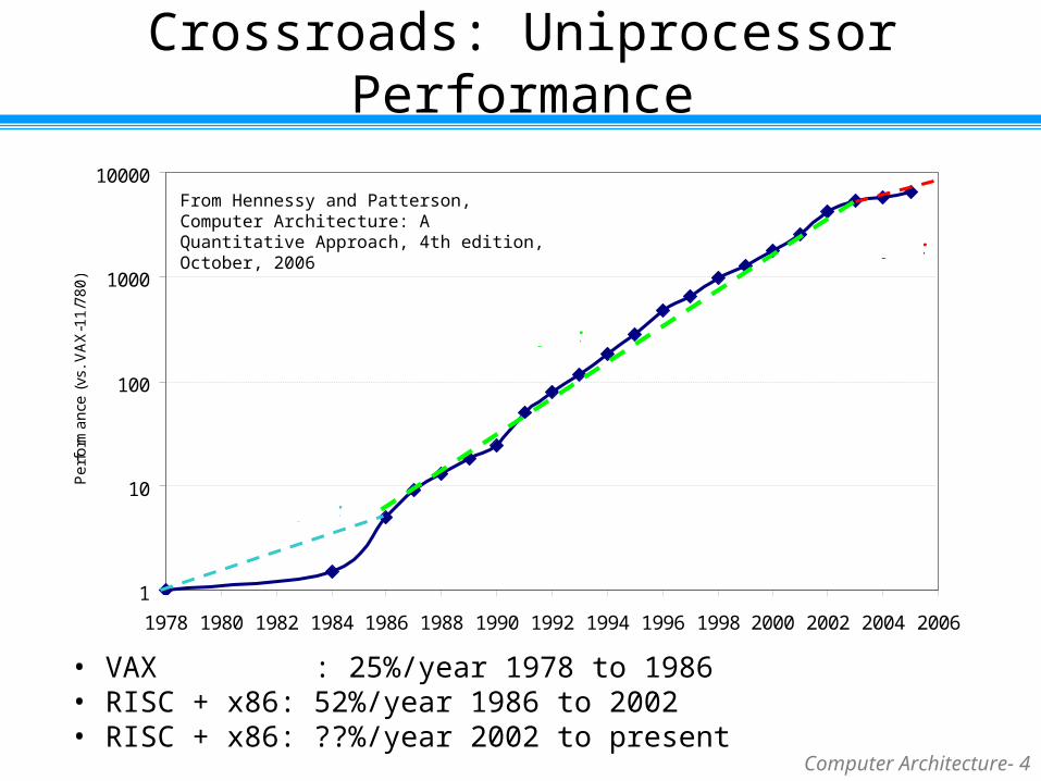
Crossroads: Uniprocessor Performance

1

10

100

1000

10000

1978 1980 1982 1984 1986 1988 1990 1992 1994 1996 1998 2000 2002 2004 2006

Pe

rfo

rma

nce

(vs

. V

AX

-11

/78

0)

25%/year

52%/year

??%/year

• VAX : 25%/year 1978 to 1986• RISC + x86: 52%/year 1986 to 2002• RISC + x86: ??%/year 2002 to present

From Hennessy and Patterson, Computer Architecture: A Quantitative Approach, 4th edition, October, 2006


Outline


Performance


1.2 Classes of Computers

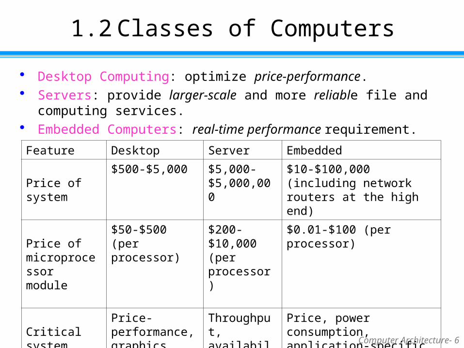
Desktop Computing: optimize price-performance. Servers: provide larger-scale and more reliable file and computing services. Embedded Computers: real-time performance requirement.

Feature Desktop Server Embedded

Price of system

$500-$5,000 $5,000-$5,000,000

$10-$100,000 (including network routers at the high end)

Price of microprocessor module

$50-$500 (per processor)

$200-$10,000 (per processor)

$0.01-$100 (per processor)

Critical system design issues

Price-performance, graphics performance

Throughput, availability, scalability

Price, power consumption, application-specific performance


Outline


Performance


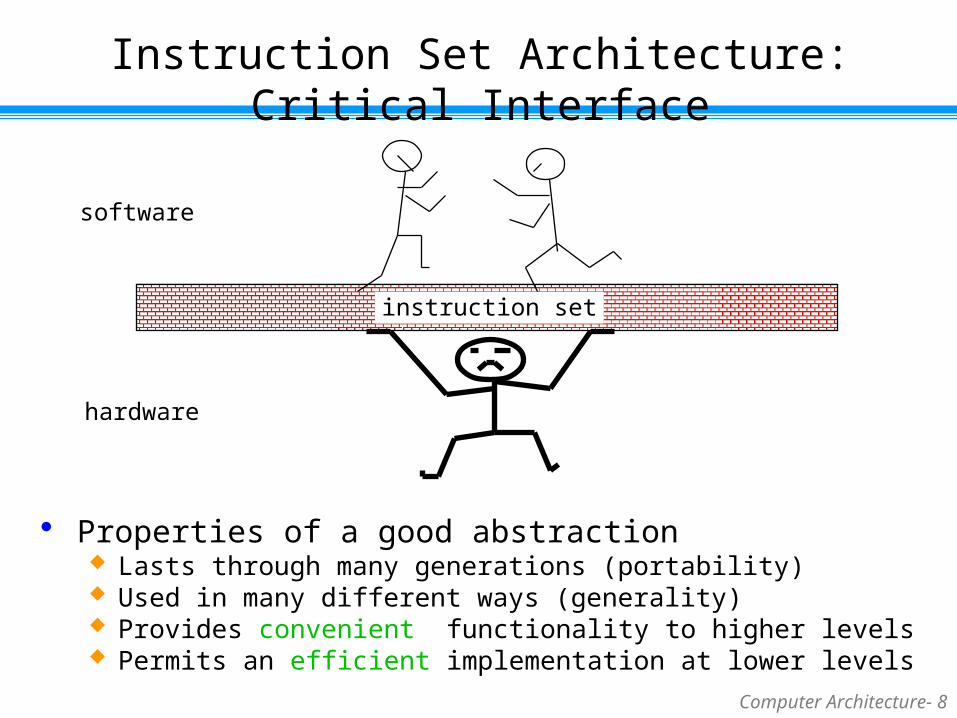
Instruction Set Architecture: Critical Interface

Properties of a good abstraction Lasts through many generations (portability) Used in many different ways (generality) Provides convenient functionality to higher levels Permits an efficient implementation at lower levels

instruction set

software

hardware


Instruction Set Architecture (ISA)

ISA is the actual programmer-visible instruction set. Class of ISA; Memory addressing; Addressing modes; Types and sizes of operands; Operations; Control flow instructions; Encoding on ISA.


Organization, Hardware, and Architecture

Organization: includes the high-level aspects of a computer’s design. Memory system, the memory interconnect, and the design of the internal

processor or CPU (arithmetic, logic, branching, and data transfer). For example: AMD Opteron 64 and Intel P4 have same ISA, but they have

different internal pipeline and cache organizations.

Hardware: detailed logic design and the packaging technology. For example, P4 and Mobile P4 have same ISA and organization, but they

have different clock frequency and memory system.

Architecture: covers all three aspects of computer design – instruction set architecture, organization, and hardware. Designer must meet functional requirements as well as price, power,

performance, and availability goals.


Outline


Performance


1.4 Trends in Technology

A successful new ISA may last decades, for example, IBM mainframe.

Four critical technologies Integrated circuit logic technology: transistor density increased by about

35% per year, quadrupling in somewhat over four years; Semiconductor DRAM (Dynamic Random-Access Memory): capacity

increases by about 40% per year, doubling roughly every two years; Magnetic disk technology: roller coaster of rates, disk are 50-100 times

cheaper per bit than DRAM (chapter 6). Network technology: network performance depends both on the

performance of switches and transmission.


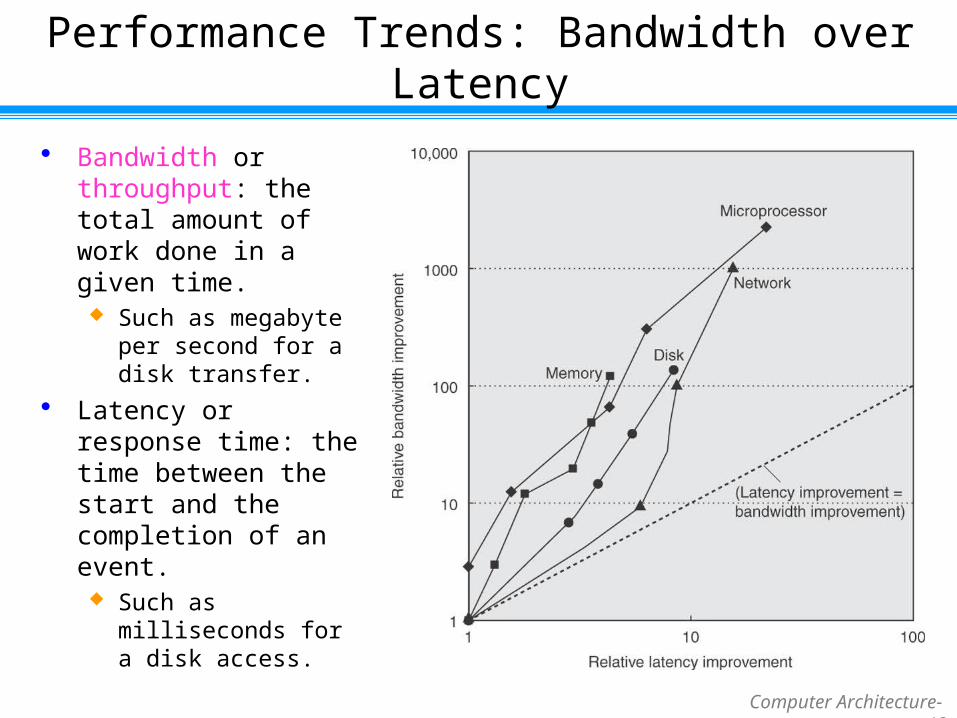
Performance Trends: Bandwidth over Latency

Bandwidth or throughput: the total amount of work done in a given time. Such as megabyte per

second for a disk transfer.

Latency or response time: the time between the start and the completion of an event. Such as milliseconds for

a disk access.


Scaling of Transistor Performance and Wires

Feature size: the minimum size of a transistor or a wire in either the x or y dimension. From 10 microns in 1971 to 0.09 microns (90 nm) in 2006; The density of transistors increases quadratically with a linear decrease in

feature size; Transistor performance improves linearly with decreasing feature size; Since improvement in transistor density, thus CPU move quickly from 4-

bit to 8-bit, to 16-bit, to 32-bit microprocessors; However, the signal delay for a wire increases in proportion to the

production of its resistance and capacitance.


Outline


Performance


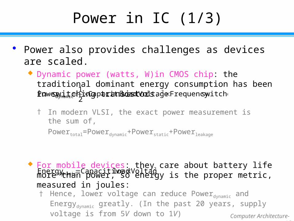
Power in IC (1/3)

Power also provides challenges as devices are scaled. Dynamic power (watts, W)in CMOS chip: the traditional dominant energy

consumption has been in switching transistors.

For mobile devices: they care about battery life more than power, so energy is the proper metric, measured in joules:

switchedFrequency Voltageload Capacitive2

1Power 2

dynamic

† In modern VLSI, the exact power measurement is the sum of,

Powertotal=Powerdynamic+Powerstatic+Powerleakage

2dynamic Voltageload CapacitiveEnergy

† Hence, lower voltage can reduce Powerdynamic and Energydynamic greatly. (In the past 20 years, supply voltage is from 5V down to 1V)


Power in IC (2/3)

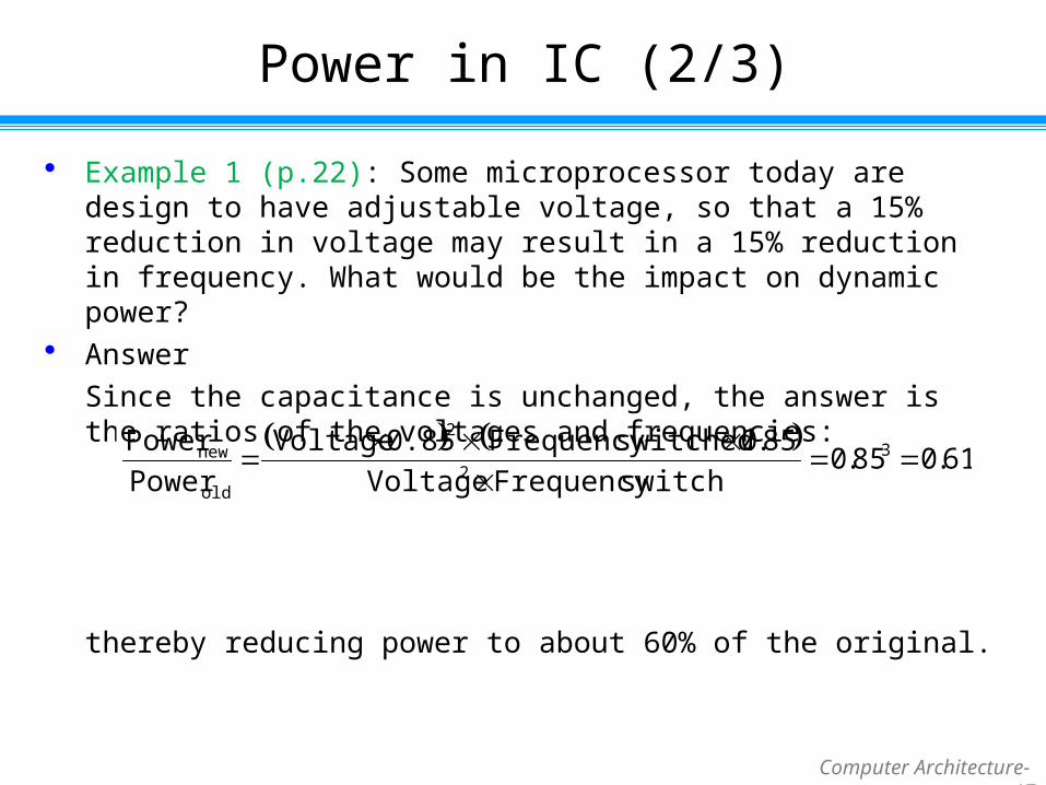
Example 1 (p.22): Some microprocessor today are design to have adjustable voltage, so that a 15% reduction in voltage may result in a 15% reduction in frequency. What would be the impact on dynamic power?

Answer

Since the capacitance is unchanged, the answer is the ratios of the voltages and frequencies:

thereby reducing power to about 60% of the original.

61.085.0

switchFrequency Voltage

85.0switchedFrequency 0.85Voltage

Power

Power 32

2

old

new


Power in IC (3/3)

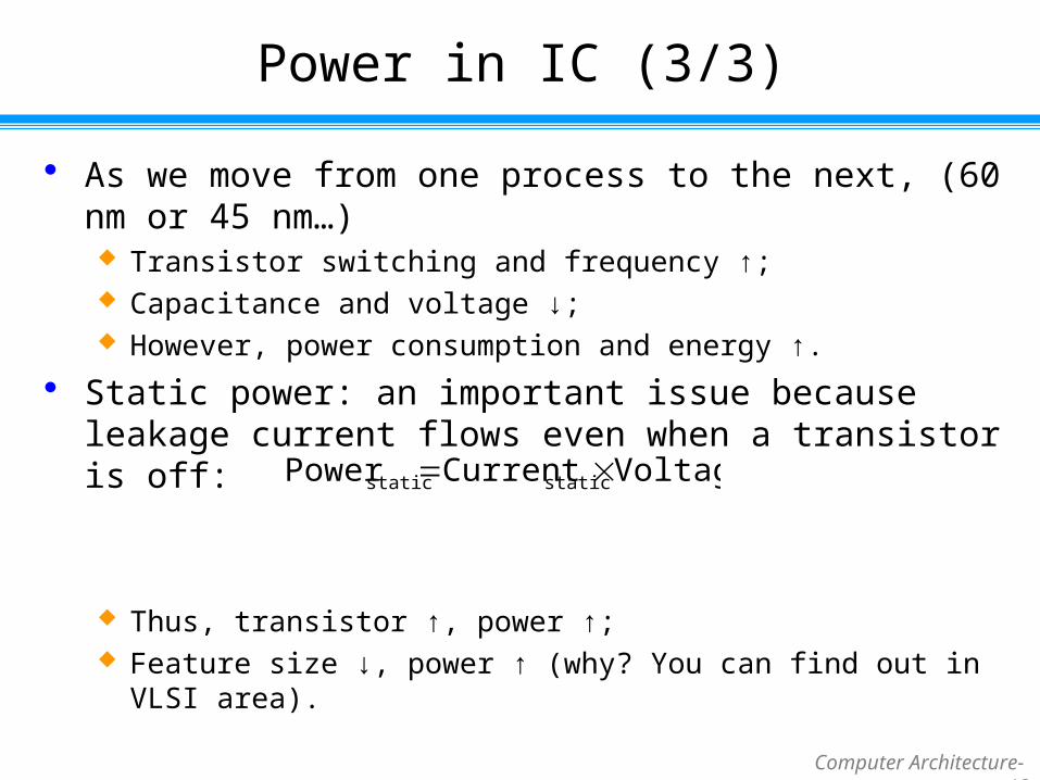
As we move from one process to the next, (60 nm or 45 nm…) Transistor switching and frequency ↑; Capacitance and voltage ↓; However, power consumption and energy ↑.

Static power: an important issue because leakage current flows even when a transistor is off:

Thus, transistor ↑, power ↑; Feature size ↓, power ↑ (why? You can find out in VLSI area).

VoltageCurrentPower staticstatic


Outline


Performance


Silicon Wafer and Dies

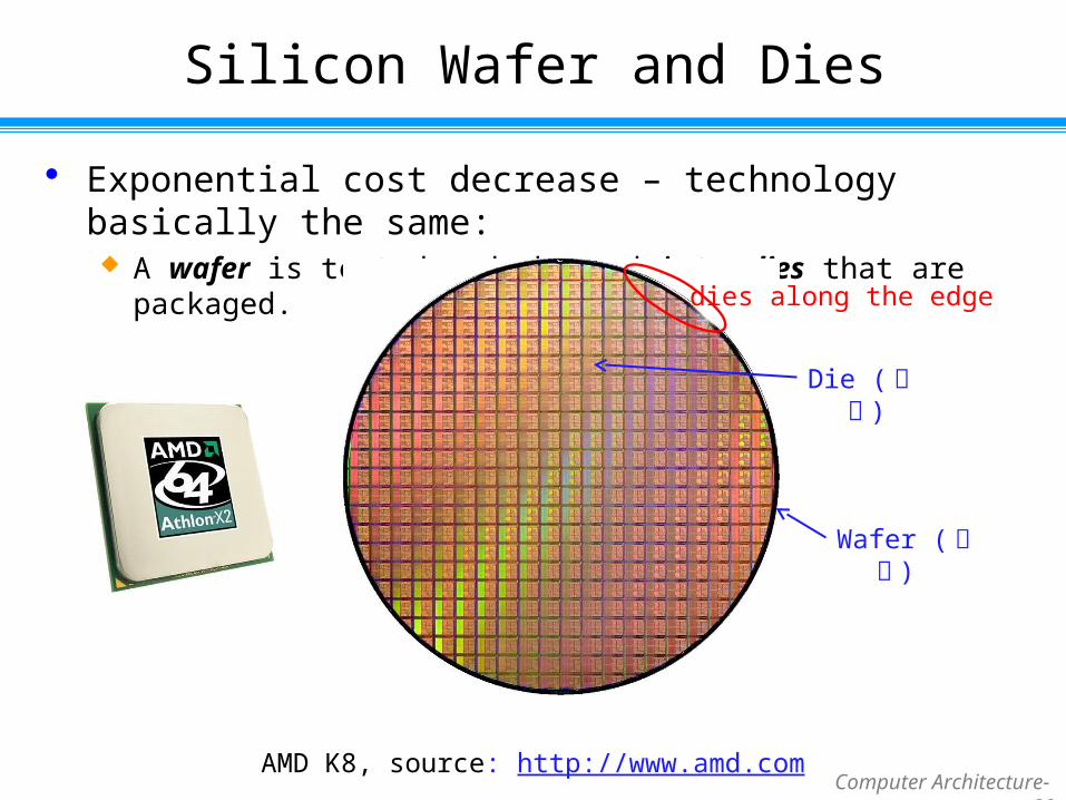
Exponential cost decrease – technology basically the same: A wafer is tested and chopped into dies that are packaged.

Die (晶粒 )

Wafer (晶圓 )

AMD K8, source: http://www.amd.com

dies along the edge


Cost of an Integrated Circuit (IC)

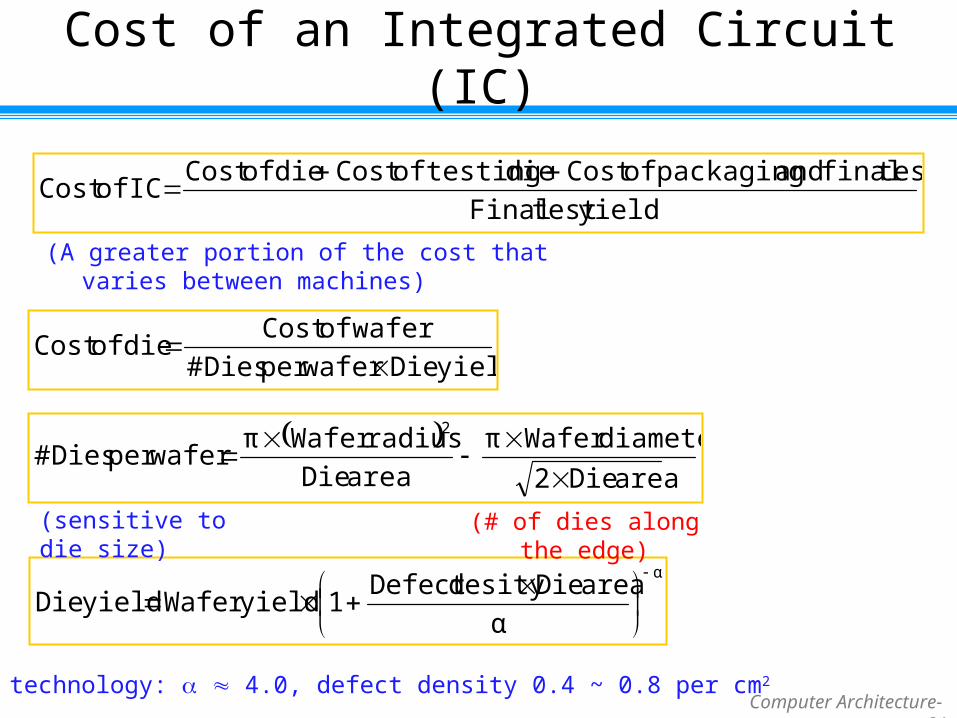
yieldDiewaferperDies#

waferofCostdieofCost

yieldtestFinal

testfinalandpackagingofCostdietestingofCostdieofCostICofCost

areaDie2

diameterWaferπ

areaDie

radiusWaferπwaferperDies#

2

α

α

areaDiedesityDefect1yieldWaferyieldDie

Today’s technology: 4.0, defect density 0.4 ~ 0.8 per cm2

(A greater portion of the cost that varies between machines)

(sensitive to die size) (# of dies along the edge)


Examples of Cost of an IC

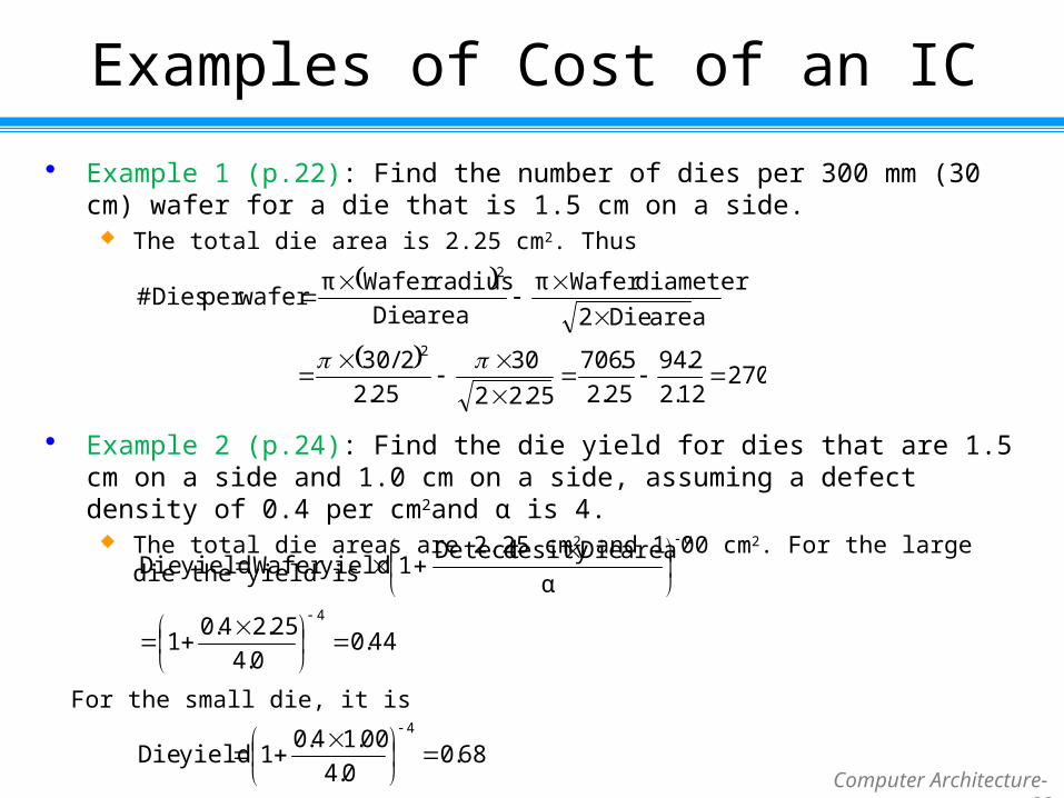
Example 1 (p.22): Find the number of dies per 300 mm (30 cm) wafer for a die that is 1.5 cm on a side.

The total die area is 2.25 cm2. Thus

Example 2 (p.24): Find the die yield for dies that are 1.5 cm on a side and 1.0 cm on a side, assuming a defect density of 0.4 per cm2and α is 4.

The total die areas are 2.25 cm2 and 1.00 cm2. For the large die the yield is

270

12.2

2.94

25.2

5.706

25.22

30

25.2

2/30

areaDie2

diameterWaferπ

areaDie

radiusWaferπwaferperDies#

2

2

44.00.4

25.24.01

α

areaDiedesityDetect1yieldWaferyieldDie

4

α

68.00.4

00.14.01yieldDie

4

For the small die, it is


Outline


Performance


Response Time, Throughput, and Performance

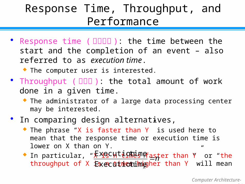
Response time (反應時間 ): the time between the start and the completion of an event – also referred to as execution time. The computer user is interested.

Throughput (流通量 ): the total amount of work done in a given time. The administrator of a large data processing center may be interested.

In comparing design alternatives, The phrase “X is faster than Y” is used here to mean that the response

time or execution time is lower on X than on Y. In particular, “X is n times faster than Y” or “the throughput of X is n

times higher than Y” will mean

nX

Y

timeExecution

timeExecution


Performance Measuring

Execution is the reciprocal of performance,

XX timeExecution

1 ePerformanc

Y

X

X

Y

X

Y

ePerformanc

ePerformanc

ePerformanc1

ePerformanc1

TimeExecution

TimeExecution n


Reliable Measure – User CPU Time

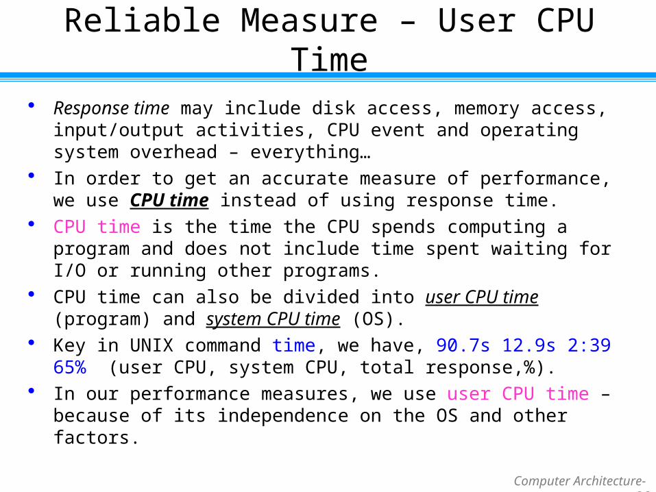
Response time may include disk access, memory access, input/output activities, CPU event and operating system overhead – everything…

In order to get an accurate measure of performance, we use CPU time instead of using response time.

CPU time is the time the CPU spends computing a program and does not include time spent waiting for I/O or running other programs.

CPU time can also be divided into user CPU time (program) and system CPU time (OS).

Key in UNIX command time, we have, 90.7s 12.9s 2:39 65% (user CPU, system CPU, total response,%).

In our performance measures, we use user CPU time – because of its independence on the OS and other factors.


Outline


Performance


Four Useful Principles of CA Design

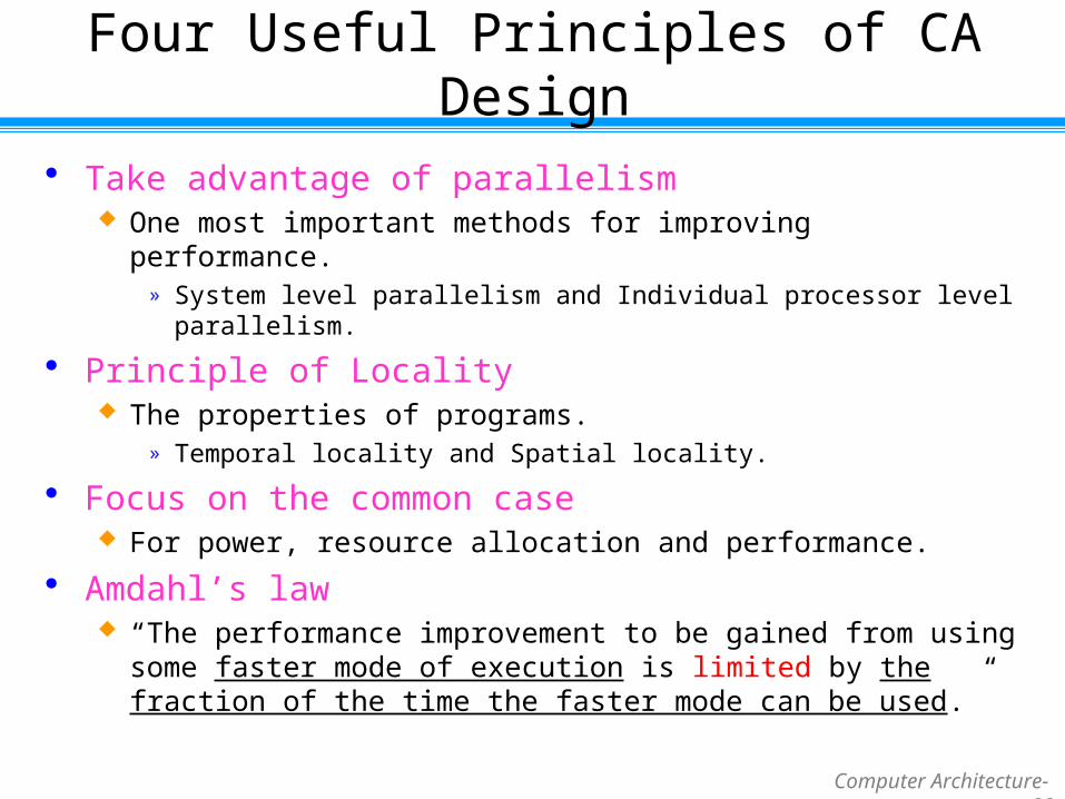
Take advantage of parallelism One most important methods for improving performance.

» System level parallelism and Individual processor level parallelism.

Principle of Locality The properties of programs.

» Temporal locality and Spatial locality.

Focus on the common case For power, resource allocation and performance.

Amdahl’s law “The performance improvement to be gained from using some faster mode

of execution is limited by the fraction of the time the faster mode can be used.”


Two Equations to Evaluate Alternatives

Amdahl’s Law The performance gain that can be obtained by improving some porting of

a computer can be calculated using Amdahl’s Law. Amdahl’s Law defines the speedup that can be gained by using a

particular feature.

The CPU Performance Equation Essentially all computers are constructed using a clock running at a

constant rate. CPU time then can be expressed by the amount of clock cycles.


Amdahl's Law (1/5)

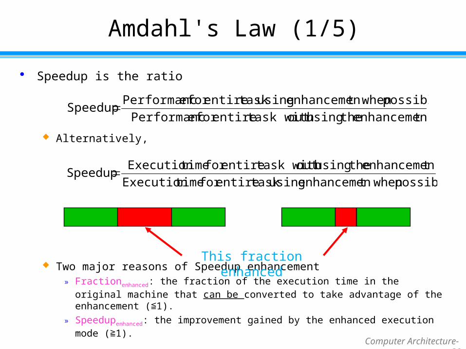
Speedup is the ratio

Alternatively,

Two major reasons of Speedup enhancement» Fractionenhanced: the fraction of the execution time in the original machine that can be

converted to take advantage of the enhancement ( 1).≦» Speedupenhanced: the improvement gained by the enhanced execution mode ( 1).≧

tenhancemen theusingout task withentirefor ePerformanc

possiblet when enhancemen using task entirefor ePerformancSpeedup

This fraction enhanced

possiblet when enhancemen using task entirefor timeExecution

t enhancemen theusingout task withentirefor timeExecution Speedup


Amdahl's Law (2/5)

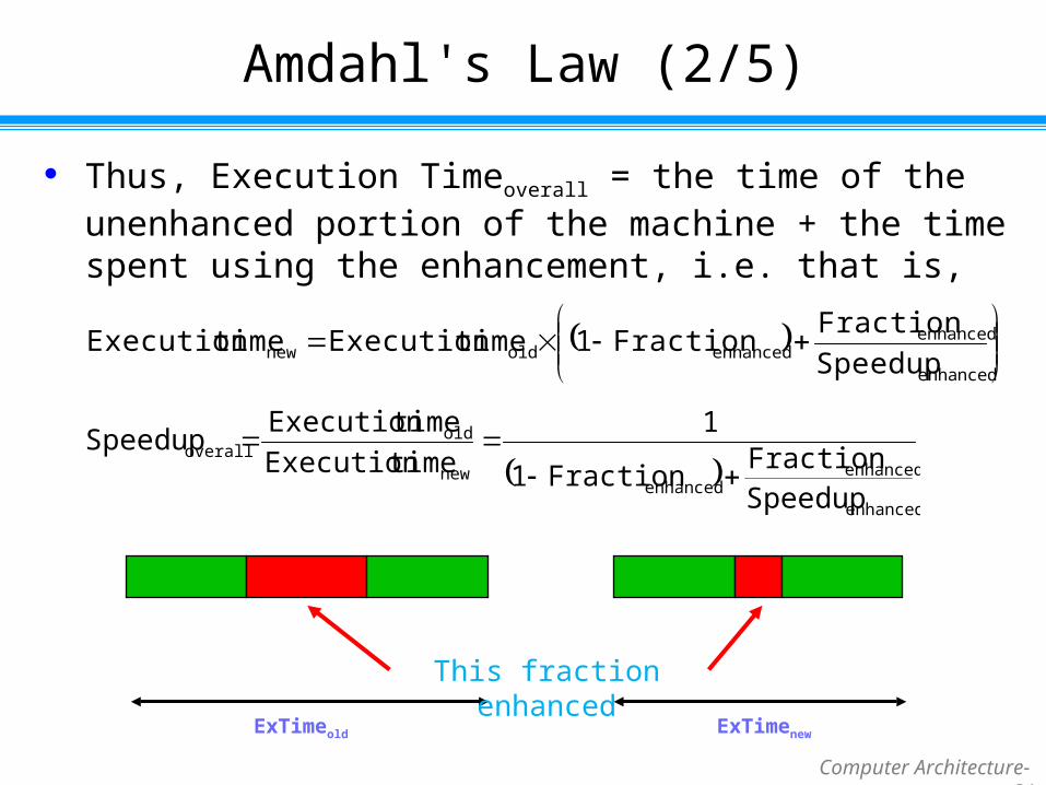
Thus, Execution Timeoverall = the time of the unenhanced portion of the machine + the time spent using the enhancement, i.e. that is,

ExTimeold ExTimenew

enhanced

enhancedenhancedoldnew Speedup

FractionFraction1timeExecutiontimeExecution

enhanced

enhancedenhanced

new

oldoverall

SpeedupFraction

Fraction1

1

timeExecution

timeExecutionSpeedup

This fraction enhanced


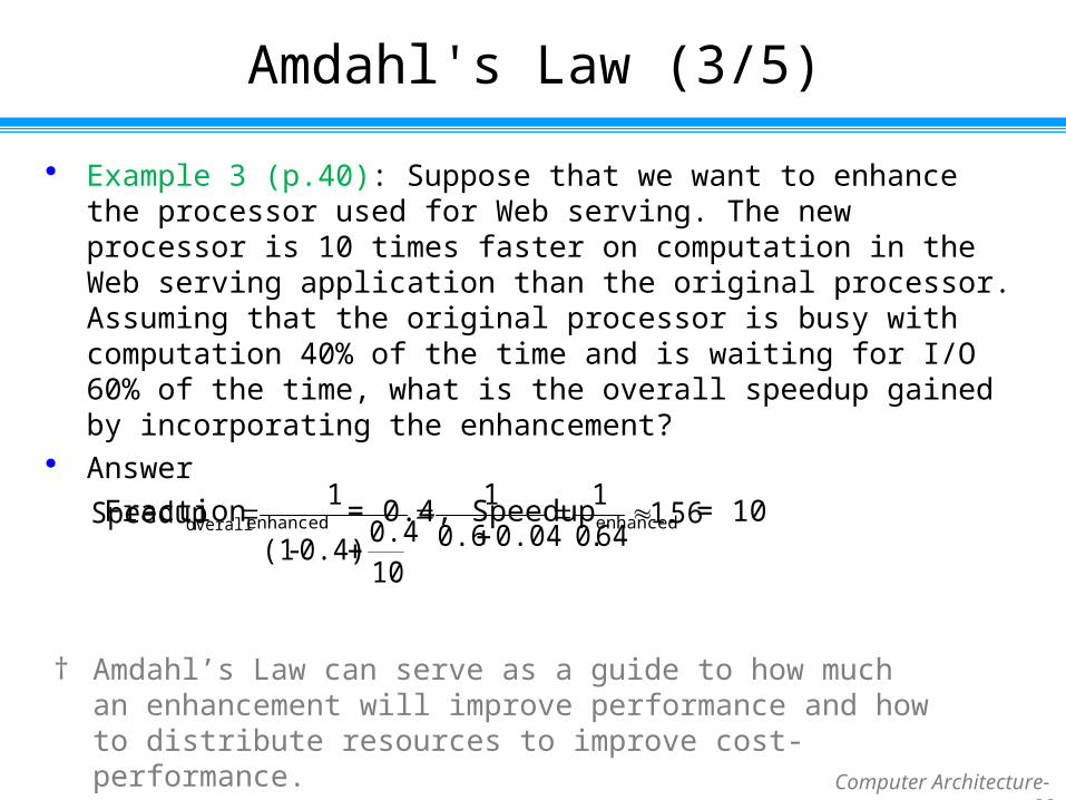
Amdahl's Law (3/5)

Example 3 (p.40): Suppose that we want to enhance the processor used for Web serving. The new processor is 10 times faster on computation in the Web serving application than the original processor. Assuming that the original processor is busy with computation 40% of the time and is waiting for I/O 60% of the time, what is the overall speedup gained by incorporating the enhancement?

Answer

Fractionenhanced = 0.4, Speedupenhanced = 10

56.164.0

1

0.040.6

1

100.4

0.4)-(1

1Speedupoverall

† Amdahl’s Law can serve as a guide to how much an enhancement will improve performance and how to distribute resources to improve cost-performance.


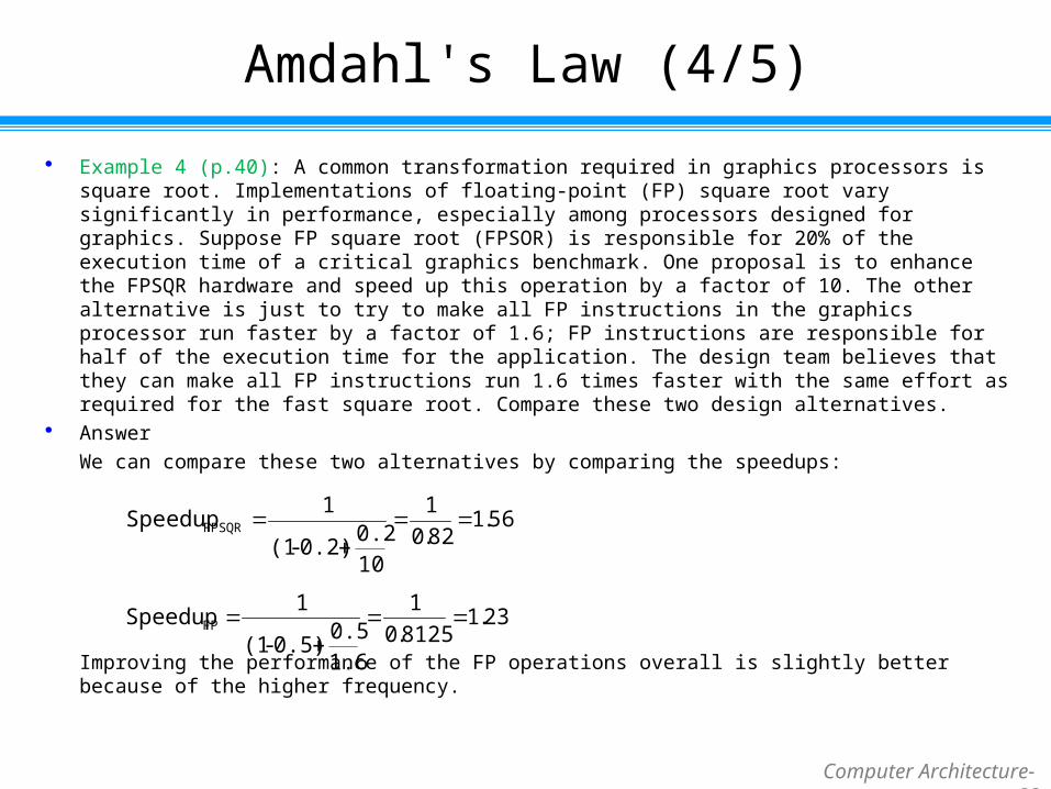
Amdahl's Law (4/5)

Example 4 (p.40): A common transformation required in graphics processors is square root. Implementations of floating-point (FP) square root vary significantly in performance, especially among processors designed for graphics. Suppose FP square root (FPSOR) is responsible for 20% of the execution time of a critical graphics benchmark. One proposal is to enhance the FPSQR hardware and speed up this operation by a factor of 10. The other alternative is just to try to make all FP instructions in the graphics processor run faster by a factor of 1.6; FP instructions are responsible for half of the execution time for the application. The design team believes that they can make all FP instructions run 1.6 times faster with the same effort as required for the fast square root. Compare these two design alternatives.

Answer

We can compare these two alternatives by comparing the speedups:

Improving the performance of the FP operations overall is slightly better because of the higher frequency.

56.182.0

1

100.2

0.2)-(1

1SpeedupFPSQR

23.18125.0

1

1.60.5

0.5)-(1

1SpeedupFP


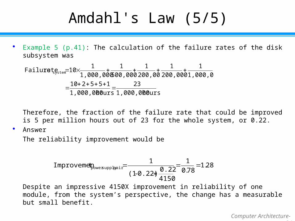
Amdahl's Law (5/5)

Example 5 (p.41): The calculation of the failure rates of the disk subsystem was

Therefore, the fraction of the failure rate that could be improved is 5 per million hours out of 23 for the whole system, or 0.22.

Answer

The reliability improvement would be

Despite an impressive 4150X improvement in reliability of one module, from the system’s perspective, the change has a measurable but small benefit.

28.178.0

1

4150

0.220.22)-(1

1tImprovemen pairsupply power

hours 1,000,000

23

hours 1,000,000

155210

1,000,000

1

200,000

1

200,00

1

500,000

1

1,000,000

110rate Failure system


CPU Performance (1/5)

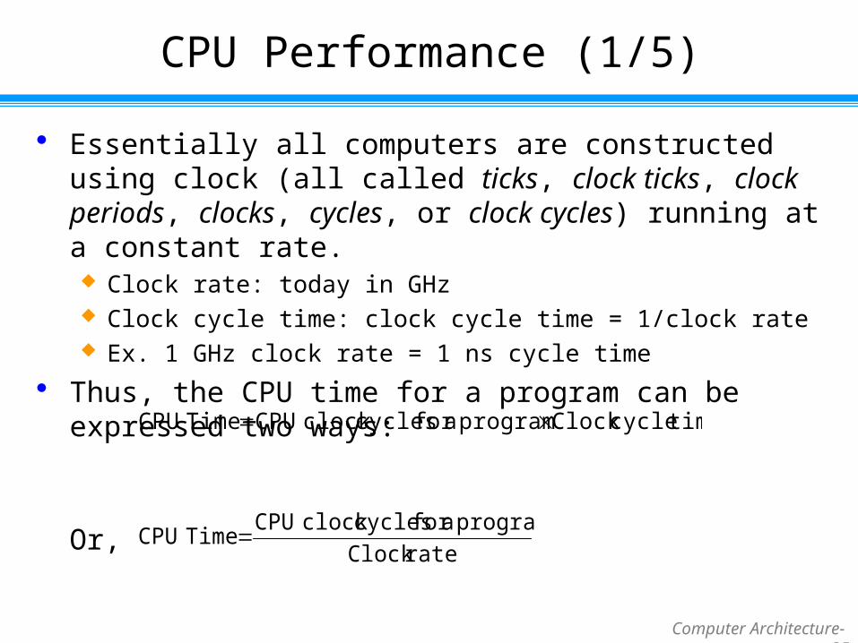
Essentially all computers are constructed using clock (all called ticks, clock ticks, clock periods, clocks, cycles, or clock cycles) running at a constant rate. Clock rate: today in GHz Clock cycle time: clock cycle time = 1/clock rate Ex. 1 GHz clock rate = 1 ns cycle time

Thus, the CPU time for a program can be expressed two ways:

Or,

timecycleClock program afor cyclesclock CPUTime CPU

rateClock

program afor cyclesclock CPU Time CPU



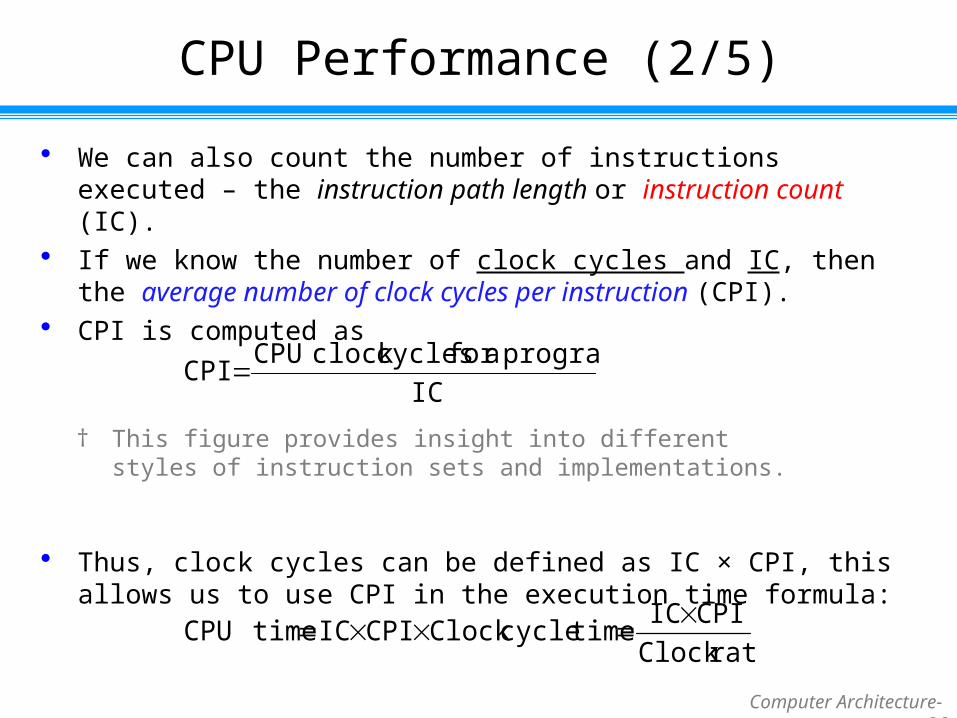
We can also count the number of instructions executed – the instruction path length or instruction count (IC).

If we know the number of clock cycles and IC, then the average number of clock cycles per instruction (CPI).

CPI is computed as

Thus, clock cycles can be defined as IC × CPI, this allows us to use CPI in the execution time formula:

IC

program afor cyclesclock CPU CPI

† This figure provides insight into different styles of instruction sets and implementations.

rateClock

CPIIC timecycleClock CPIIC timeCPU



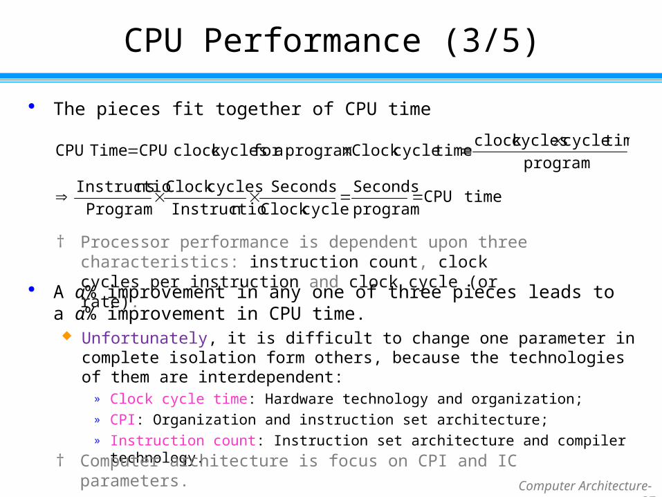
The pieces fit together of CPU time

A α% improvement in any one of three pieces leads to a α% improvement in CPU time. Unfortunately, it is difficult to change one parameter in complete isolation form

others, because the technologies of them are interdependent:» Clock cycle time: Hardware technology and organization;» CPI: Organization and instruction set architecture;» Instruction count: Instruction set architecture and compiler technology.

timeCPUprogram

Seconds

cycleClock

Seconds

nInstructio

cyclesClock

Program

nsInstructio

program

timecyclecyclesclock timecycleClock program afor cyclesclock CPUTime CPU

† Processor performance is dependent upon three characteristics: instruction count, clock cycles per instruction and clock cycle (or rate).

† Computer architecture is focus on CPI and IC parameters.



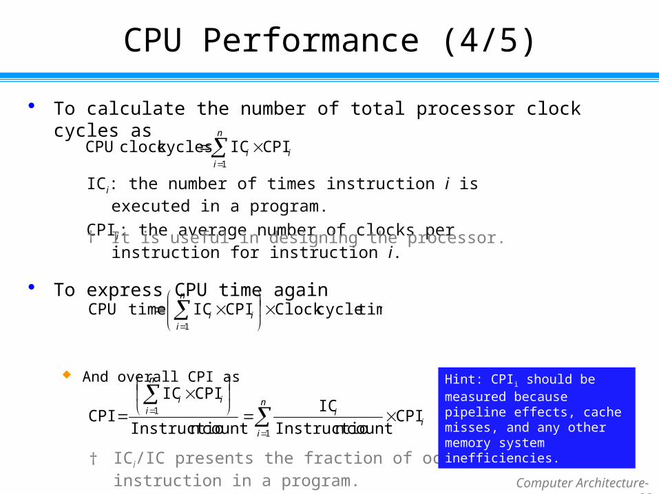
To calculate the number of total processor clock cycles as

To express CPU time again

And overall CPI as

i

n

ii CPIICcyclesclock CPU

1

ICi: the number of times instruction i is executed in a program.

CPIi: the average number of clocks per instruction for instruction i.

† ICi/IC presents the fraction of occurrences of that instruction in a program.

† It is useful in designing the processor.

timecycleClock CPIIC timeCPU1

i

n

ii

n

ii

ii

n

ii

1

1 CPIcountn Instructio

IC

countn Instructio

CPIIC

CPI

Hint: CPIi should be measured because pipeline effects, cache misses, and any other memory system inefficiencies.



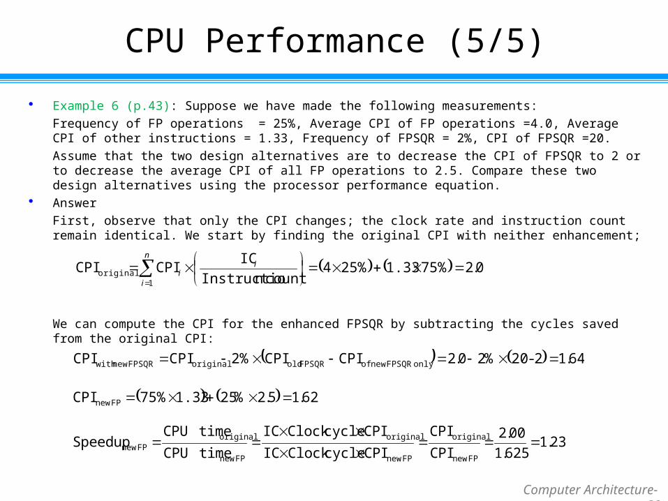
Example 6 (p.43): Suppose we have made the following measurements:

Frequency of FP operations = 25%, Average CPI of FP operations =4.0, Average CPI of other instructions = 1.33, Frequency of FPSQR = 2%, CPI of FPSQR =20.

Assume that the two design alternatives are to decrease the CPI of FPSQR to 2 or to decrease the average CPI of all FP operations to 2.5. Compare these two design alternatives using the processor performance equation.

Answer

First, observe that only the CPI changes; the clock rate and instruction count remain identical. We start by finding the original CPI with neither enhancement;

We can compute the CPI for the enhanced FPSQR by subtracting the cycles saved from the original CPI:

0.275%1.3325%4countn Instructio

ICCPICPI

1original

n

i

ii

64.12-20%20.2CPICPI2%CPICPI only FPSQR new ofFPSQR oldoriginalFPSQR newwith

62.15.2%251.3375%CPI FP new

23.1625.1

00.2

CPI

CPI

CPIcycleClock IC

CPIcycleClock IC

timeCPU

timeCPUSpeedup

FP new

original

FP new

original

FP new

originalFP new


Amdahl's Law vs. CPU Performance

CPU performance equation is better than Amdahl’s Law Possible to measure the constituent parts; To measure the fraction of execution time for which a set of instructions is

responsible; For an existing processor, to measure execution time and clock speed is

easy; The challenge lies in discovering the instruction count or the CPI.

» Most new processors include counter for both instructions executed and for clock cycles.

Documents

Computer Architecture- 1 Ping-Liang Lai ( 賴秉樑 ) Chapter 1 Fundamentals of Computer Design Computer Architecture 計算機結構