OPEN ACCESS

Concatenated tensor network statesTo cite this article: R Hübener et al 2010 New J. Phys. 12 025004

 

View the article online for updates and enhancements.

Related contentFundamentals of universality in one-wayquantum computationM Van den Nest, W Dür, A Miyake et al.

-

Renormalization and tensor product statesin spin chains and latticesJ Ignacio Cirac and Frank Verstraete

-

Homogeneous multiscale entanglementrenormalization ansatz tensor networks forquantum critical systemsM Rizzi, S Montangero, P Silvi et al.

-

Recent citationsA tensor-network-based big data fusionframework for Cyber-Physical-SocialSystems (CPSS)Shunli Zhang et al

-

Maolin Wang et al-

Predicting toxicity by quantum machinelearningTeppei Suzuki and Michio Katouda

-

This content was downloaded from IP address 119.239.76.248 on 20/09/2021 at 01:10

T h e o p e n – a c c e s s j o u r n a l f o r p h y s i c s

New Journal of Physics

Concatenated tensor network states

R Hübener1, V Nebendahl1 and W Dür1,2

1 Institut für Theoretische Physik, Universität Innsbruck, Technikerstraße 25,A-6020 Innsbruck, Austria2 Institut für Quantenoptik und Quanteninformation der ÖsterreichischenAkademie der Wissenschaften, Otto Hittmair-Platz 1, A-6020 Innsbruck,AustriaE-mail: robert.huebener@uibk.ac.at

New Journal of Physics 12 (2010) 025004 (28pp)Received 19 May 2009Published 26 February 2010Online at http://www.njp.org/doi:10.1088/1367-2630/12/2/025004

Abstract. We introduce the concept of concatenated tensor networksto efficiently describe quantum states. We show that the correspondingconcatenated tensor network states can efficiently describe time evolution andpossess arbitrary block-wise entanglement and long-ranged correlations. Weillustrate the approach for the enhancement of matrix product states, i.e. one-dimensional (1D) tensor networks, where we replace each of the matrices of theoriginal matrix product state with another 1D tensor network. This procedureyields a 2D tensor network, which includes—already for tensor dimension2—all states that can be prepared by circuits of polynomially many (possiblynon-unitary) two-qubit quantum operations, as well as states resulting fromtime evolution with respect to Hamiltonians with short-ranged interactions.We investigate the possibility of efficiently extracting information from thesestates, which serves as the basic step in a variational optimization procedure.To this aim, we utilize the known exact and approximate methods for 2D tensornetworks and demonstrate some improvements thereof, which are also applicablee.g. in the context of 2D projected entangled pair states. We generalize theapproach to higher dimensional and tree tensor networks.

New Journal of Physics 12 (2010) 0250041367-2630/10/025004+28$30.00 © IOP Publishing Ltd and Deutsche Physikalische Gesellschaft

2

Contents

1. Introduction 22. Concatenated tensor networks 3

2.1. MPS and PEPS . . . . . . . . . . . . . . . . . . . . . . . . . . . . . . . . . . 42.2. CTS . . . . . . . . . . . . . . . . . . . . . . . . . . . . . . . . . . . . . . . . 6

3. Properties of CTS 73.1. Concatenated MPS . . . . . . . . . . . . . . . . . . . . . . . . . . . . . . . . 73.2. Concatenated PEPS . . . . . . . . . . . . . . . . . . . . . . . . . . . . . . . . 113.3. Tensor tree states with internal structure . . . . . . . . . . . . . . . . . . . . . 12

4. Applications 134.1. The descriptive potential of CTS . . . . . . . . . . . . . . . . . . . . . . . . . 144.2. Reading-out information from CTS . . . . . . . . . . . . . . . . . . . . . . . . 15

5. Summary and outlook 20Acknowledgments 21Appendix A. Variational optimization of CTS-enhanced tree tensor networks 21Appendix B. Monte Carlo sampling of CTS 23References 27

1. Introduction

The classical simulation of complex quantum systems is one of the central problems in modernphysics. Given the exponential growth of the state space with the system size, such a classicalsimulation seems infeasible. However, it has been realized that the quantum systems occurringin nature often only populate a small subspace. Identifying this subspace is hence the first steptowards a successful classical simulation. For ground states of (non-critical) strongly correlatedquantum spins in a one-dimensional (1D) setup, matrix-product states (MPS) [1]–[3] turn out toprovide a proper parameterization for this subspace [4, 5]. MPS can not only efficiently describesuch ground states, but it is also possible to efficiently read out physical information from thisdescription, e.g. to compute expectation values of local observables and correlation functions.Moreover, MPS forms the basis of the density matrix renormalization group (DMRG) [6]–[8],a powerful numerical method that has been successfully applied to various problems in 1D.The relation between DMRG and MPS is an example of how the physical insight into the logicof a preparation (renormalization) procedure can be manifestly encoded into the structure of astate class.

Recent approaches to simulate ground states of strongly correlated systems in criticalsystems or higher dimensions follow a similar approach. A variety of states such as projectedentangled pairs (PEPS) [9, 10], sequentially generated states [11], string-bond states [12],weighted graph states (WGS) [13], renormalization ansatz with graph enhancement [14], orthe multiscale entanglement renormalization ansatz (MERA) [15] have been introduced withthe aim of efficiently parameterizing the relevant subspace. The entanglement properties of thecorresponding states form the guideline and determine the potential applicability of the methods.For instance, MERA can provide a logarithmic divergence for block-wise entanglement incritical 1D systems, while e.g. 2D variants of MERA as well as PEPS and string-bond statesfulfill area laws for block-wise entanglement, are typically found to be in ground states of

New Journal of Physics 12 (2010) 025004 (http://www.njp.org/)

3

2D systems. In all cases it is crucial that not only an efficient description of the states canbe obtained, but also that information can be efficiently extracted, either exactly or in anapproximate way. Based on these states, variational methods for ground state approximationand (real and imaginary) time evolution have been developed and tested. While MPS, MERAand PEPS lead to good descriptions of ground states for non-critical 1D systems, critical 1Dsystems and 2D systems, respectively, none of the proposed classes seems to be suitable forproperly describing time evolution. In fact, it has been argued that simulating time evolution isin general hard [16], as the block-wise entanglement grows—already for 1D systems—linearlyin time [17], leading quickly to a volume law. The entanglement contained in an MPS is boundedby the dimension of the matrices or tensors, and the entanglement contained in a PEPS followsan area law.

Here, we present a class of tensor network states (TNS) for which such limitations donot apply and which allow one in principle to efficiently describe states resulting from timeevolution or quantum computation. To construct these states we make use of the basic ideaunderlying previous tensor network structures. In these structures, a simplification of theexisting description can be achieved by replacing tensors of high rank (i.e. with many indices)by a network of tensors of low rank (i.e. with few indices) with appropriate topology. Thechoice of the underlying tensor network determines qualitatively different subclasses of states,in previous approaches e.g. those having a lead to MPS or PEPS when describing a 1D or 2Dstructure, respectively. We apply this idea in an iterative, or concatenated, fashion, leading toconcatenated tensor network states (CTS). That is, each of the tensors appearing in a tensornetwork is itself repeatedly replaced by another tensor network. The resulting structure is againa tensor network, similar to a PEPS, with the main difference that only some of the tensors areassociated with physical particles.

The efficient and exact extraction of information, e.g. expectation values or correlationfunctions, from an arbitrary tensor network is in general not possible, as they rely on acontraction of the network, i.e. summations over all indices of the network. Even for 2D tensornetworks, the contraction is known to be computationally hard (#P-hard) [18]. However, forcertain special cases, exact evaluation is possible. In addition, also approximate contraction andcertain Monte Carlo (MC) methods have been developed and successfully applied in the contextof 2D PEPS and imaginary time evolution [19]. We demonstrate the applicability of the estab-lished methods to the CTS and several enhancements thereof. We moreover demonstrate thatthere are novel implementations of algorithms like (imaginary) time evolution of 1D systemsand the application of quantum circuits that are more efficient in the CTS than in the MPS.

This paper is structured as follows. In section 2, we will introduce the CTS, give examplesand illustrate their properties from an analytic point of view. In section 3, we discuss theapplications of the CTS and illustrate the potential of the CTS to describe states relevant inphysics. As an example, we give the numerical treatment of a toy model; more precisely, wewill describe a state originating from the time evolution of a product state governed by the IsingHamiltonian. In section 4, we finally show several ways to extract information from a CTS,thereby utilizing and improving methods to (approximately) contract 2D tensor networks.

2. Concatenated tensor networks

In this section, we introduce the CTS and in the context of the problems having a lead to tensornetwork descriptions in general.

New Journal of Physics 12 (2010) 025004 (http://www.njp.org/)

4

(b)(a)

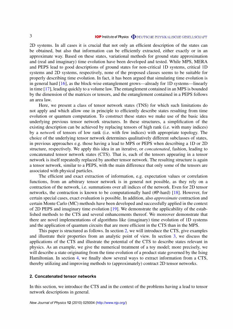
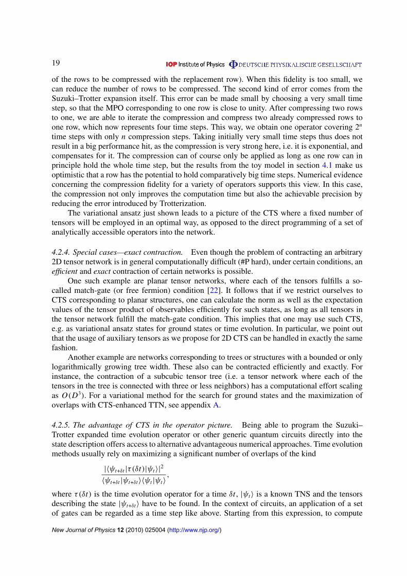
Figure 1. (a) Graphical representation of a 1D tensor network (MPS). The boxescorrespond to tensors, where shared indices are summed over. Open indicescorrespond to physical particles (red tensors). (b) Each of the tensors in theoriginal tensor network is replaced by a 1D tensor network (MPO) arranged inthe y-direction. Auxiliary tensors (no open indices) are drawn in blue. This leadsto a 2D tensor network.

A generic quantum state of N d-level systems can be written in a basis whose elementsare tensor products of basis states of the local d-level systems. The quantum state is thencharacterized by the coefficients of these basis states, which are tensors As1s2...s N of rank Nand dimension d:

|ψ〉 =

d∑s1,s2,...,sn=1

As1s2...sN |s1s2 . . . sN 〉. (1)

Hence, the description of such a state consists of d N complex parameters. This exponentialgrowth of the number of parameters used in the generic description makes it unsuitable fornumerical analysis.

2.1. MPS and PEPS

The tensor As1s2...s N of the generic description given above can be decomposed into a tensornetwork, thereby imposing a structure on this set of parameters. To do so, we will representAs1s2...s N by another set of tensors of smaller rank. Some of the indices of the small-rank tensorscorrespond to the state of a physical site {s1, s2, . . . , sN } as before. The remaining auxiliaryindices are shared between pairs of the small-rank tensors, and to recover the coefficient of abasis state of the physical system, the shared indices will be contracted, i.e. summed over. Theinformation that tensors share indices can be represented by a graph, where ‘tensors’ correspondto vertices and ‘sharing an index’ corresponds to an edge. The indices corresponding to physicalstates will in the following be called open. We will furthermore use Greek letters α j , βk , etc torefer to shared indices, while open indices will be denoted by s j .

As an example, one may use a 1D structure for the tensor network, leading to MPS (seefigure 1(a))

As1s2...sN =

D∑α1,α2,...αN =1

A[s1]α1

A[s2]α1α2

. . . A[sN−1]αN−2αN−1

A[sN ]αN−1

, (2)

which are described by the tensors A[si ]αiαi+1

and A[s1]α1, A[s N ]

αN. For a fixed choice of s1s2 . . . sN , the

coefficient As1s2...s N is obtained by calculating the product of the D × D matrices A[si ]αiαi+1

(except

New Journal of Physics 12 (2010) 025004 (http://www.njp.org/)

5

(b)(a)

(d)(c)

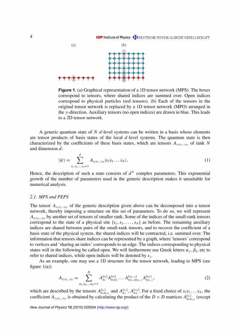
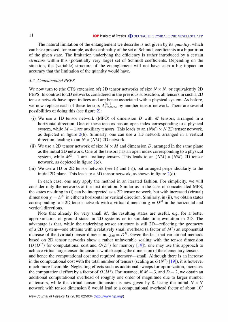
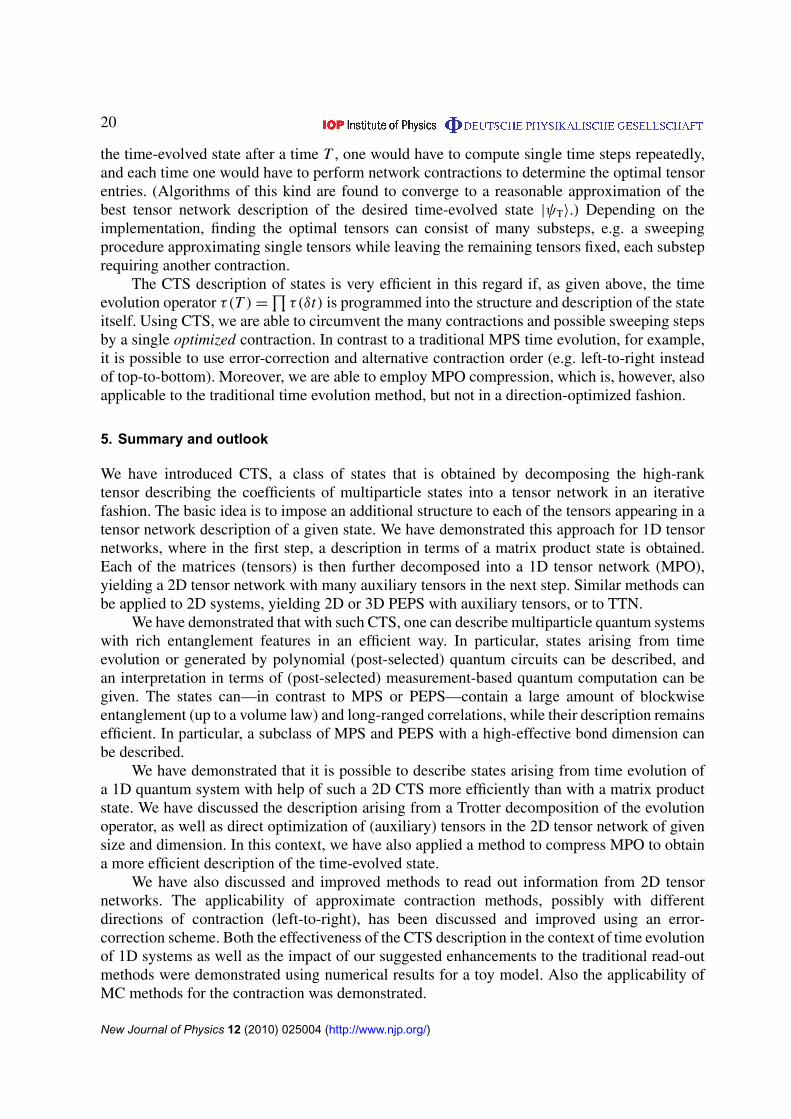
Figure 2. Examples of concatenated 2D TNS. The boxes correspond to tensors,where joint indices are summed over. Open indices correspond to physicalparticles (red tensors), while auxiliary tensors (no open indices) are drawn inblue. (a) Original 2D tensor network, where each of the tensors correspondsto a physical particle. (b) Each of the original tensors is replaced by a 1Dtensor network (MPS, consisting of three tensors, two of which are auxiliarytensors) in the horizontal direction. (c) Each of the original tensors is replacedby a 2D tensor network (of size 3 × 3) arranged in the same plane as theoriginal 2D tensor network. (d) Each of the initial tensors is replaced by an MPSperpendicular to the original plane (the z-direction). This leads to a 3D tensornetwork structure.

at the border, where one has vectors A[si ]αi

). By choosing D large enough (but still D � d N ),one can represent any tensor and hence any quantum state in this form. A restriction to small Dallows one to describe a certain subset of states efficiently.

In a similar way, one can consider tensor network structures with different topologies andhigher dimensional connectivity. If the physical system consists of particles on a 2D regularlattice, the procedure analogous to the construction of the MPS described above yields a 2Dregular tensor grid, e.g.

As1s2...s9 =

D∑greek indices=1

A[s1]α1,β1

A[s2]α1α2β2

A[s3]α2β3

A[s4]β1α3β4

A[s5]α3β2α4β5

A[s6]β3α4β6

A[s7]β4α5

A[s8]α5β5α6

A[s9]α6β6,

the structure corresponding to the PEPS in 2D (see figure 2(a)).Tensor networks that have been subjected to detailed investigation include 1D graphs with

and without periodic boundary conditions (MPS), trees [20, 21] and 2D lattices (PEPS) [9].Investigations of networks of different topologies have shown that 1D and tree-like structures

New Journal of Physics 12 (2010) 025004 (http://www.njp.org/)

6

are generally easy to simulate numerically. Tensor networks corresponding to graphs with manyloops, on the other hand, are generally hard to simulate [20, 21], and only in special casesefficient algorithms are known, see e.g. [22]. Some of the networks, e.g. corresponding toa 2D lattice, are even known to correspond to states being resources of measurement-basedquantum computation (MQC) and hence (having a generally applicable method) to treat theseTNS numerically efficiently and exactly would mean to efficiently simulate a quantum computerclassically. In fact, the contraction of such 2D networks was proven to be a computationally hardproblem in general [23].

2.2. CTS

We will consider concatenated tensor networks in the following. That is, given a tensor networkas in the previous subsections, we will replace each individual tensor in the network byanother tensor network. This can in principle be carried out in an iterative way, leading toconcatenated tensor structures. We will typically only consider tensor networks stemming froma few iterations, given the fact that the total number of tensors increases exponentially with thenumber of iterations. Note that most of the additional tensors that we introduce will be auxiliarytensors, i.e. without open indices and hence not corresponding to quantum systems. We alsoremark that it is not necessary to use the same tensor structure at each concatenation level.

The structure that we finally obtain is again a (possibly high-dimensional) tensor network.As long as the total number of tensors, as well as their rank and dimension, is polynomiallybounded, we obtain a class of states that can be described by a polynomial number ofparameters, i.e. efficiently. We call the family of quantum states that can be described in thisway CTS.

A key element of this approach is to impose an internal structure on the tensor descriptionbeing used, thereby reducing the information content, while its ability to describe entanglementis in principle still kept. This allows one to describe states with a large amount of block-wiseentanglement, up to a volume law, and long-ranged correlations using only small rank tensorsof small dimension at the elementary level.

By construction, the imposed structure is similar to the one behind the verysuccessful DMRG method. Independently of this ancestry of the ansatz, there are someilluminating interpretations going beyond the DMRG picture3. Different from the DMRG, therenormalization structure in the concatenated tensor networks is not necessarily realized in a

3 The TNS that generically correspond to the DMRG are the MPS. The matrices used in the MPS encode arule for coarse-graining over subsystems of the whole spin system. That means, the matrices (or tensors) areused to identify a relevant small subspace of a subsystem of several contiguous sites, eventually allowing for asimplification of the description by concentrating on their important features. Naturally, the selected subsystemsresult from a spacial division of the spin system. However, also a single particle transferred through time by thesubsequent application of operators (tensors) can be interpreted as a system consisting of several parts, namelythe single site at different times. Accordingly, a coarse-graining procedure performed ‘over time’ is applicable inthis case. The CTS description of a multipartite spin system allows for both, timely and spatial, coarse-grainingprocedures. If one of them has favorable correlation properties, as far as an MPS description is concerned, it isadvantageous to use this anisotropy in the tensor network. For instance, the read-out process (see section 4.2.1),relying on intermediate MPS descriptions, is a situation where knowledge about such a favorable renormalizationdirection can be exploited. This is the reason why, when reading out the information from 2D rectangular CTS,going from left-to-right is sometimes more precise than going from top-to-bottom.

New Journal of Physics 12 (2010) 025004 (http://www.njp.org/)

7

spatial fashion (i.e. renormalization by coarse-graining over several contiguous sites), but—being subject to interpretation and depending on the actual network—in a timely fashion (i.e. bycoarse-graining over the same particle state over different times). This timely renormalizationstructure is implemented via tensors stemming from the operator-based formulation of aSuzuki–Trotter expansion, or going further, as state-preparing applications of generic operators,reflecting an intrinsic symmetry when interchanging time and space in the description.

We find that already with a 2D network of size poly(N ) and tensor dimension 2, all statesthat can be prepared by a polynomially sized quantum circuit can be represented as CTS.Furthermore, the picture that the CTS stems from a preparation using MQC is possible. Allthese interpretations are suited to inspire further development and nurture some hope that thedescribed state class might—by virtue of its construction—be suited for a good description oftime-evolved states or quantum circuits.

3. Properties of CTS

In the following, we give a number of examples of CTS and discuss their properties.

3.1. Concatenated MPS

We now consider concatenated MPS. We start with a 1D tensor network as shown in figure 1(a),and replace each of the tensors A[sk ]

αkαk+1by a 1D tensor network, as shown in figure 1(b). More

precisely, each matrix A[sk ]αkαk+1

for sk = 1, 2, . . . , d is replaced by a matrix product operator(MPO) [24],

A[sk ]αkαk+1

↔

Dk∑β1,β2,...,βM=1

A[sk ]α1

kα1k+1β1

Bα2kα

2k+1β1β2

. . . BαMk α

Mk+1βM

. (3)

and the indices αk are replaced by α jk ∈ (1, 2, . . . , D) corresponding to several connections to

the neighboring tensors. Note that the effective dimension of all these connections togetheris given by χ =

∏k Dk . In this way, we obtain a 2D tensor network, where only N tensors

A[sk ] have open indices and correspond to physical sites, while there are (N − 1)M auxiliarytensors B. The process of replacing individual tensors by 1D tensor networks can be iterated.At the next level, one obtains a 3D tensor network and so forth. We remark that one mayalso consider 2D tensor networks with periodic boundary conditions, either in the horizontalor vertical direction.

In the following, we will consider 2D tensor networks (i.e. only the first iteration level) ofsize N × M with M = poly(N ). We analyze the states that can be described by such a CTS, andstudy their entanglement features. We show that

• All states that can be created by a polynomially sized quantum circuit can be efficientlydescribed by such a 2D CTS with Dk = 2. This includes unitary quantum circuits as wellas post-selected quantum circuits.

• All states resulting from a time evolution for a time t with respect to short-rangeHamiltonians can be efficiently described by an N × M 2D CTS, where M scales quad-ratically with time t .

• A subclass of MPS with an effective bond dimension of the order of χ = DMk can be

described efficiently by an N × M 2D CTS.

New Journal of Physics 12 (2010) 025004 (http://www.njp.org/)

8

Regarding the entanglement features, we show

• The block-wise entanglement of an N × M 2D CTS can be O(M). In particular, stateswith a volume law for block-wise entanglement and with long-ranged correlations can bedescribed efficiently.

3.1.1. Interpretation in terms of (post-selected) quantum circuits. Here we show that for aspecific choice of tensors, the 2D tensor network can be interpreted as a quantum circuitconsisting of generic gates. We consider a quantum circuit for N qubits of depth M =

O(poly(N )). We find that one can describe the resulting state from such a quantum computationby a 2D tensor network of size of the order of O(N × M), i.e. of polynomially many tensors,where the tensor dimension is D = 2. Let us now demonstrate how a standard quantum circuitconsisting of arbitrary single-qubit rotations and two-qubit phase gates—which constitute auniversal gate set—can be encoded into the tensor network. We denote the auxiliary tensorsby B(i, j)

αlαrαuαdand the ones connected to physical particles by A(i, j)

αlαrαusd(typically), where the

subindices l, r, u and d stand for left, right, up and down, and i and j are labels that indicate theposition of the tensor in the 2D tensor network (i th row and j th column). The uppermost line oftensors B(1, j)

αlαrαdhave no ‘up’ index, and similarly the tensors at the border do not have left/right

indices. We identify each horizontal line of tensors with a certain time step in the circuit, and thefirst (uppermost) line is used to initialize the input state to |0〉

⊗N (or some other product state),while the last line corresponds to the output state.

Initialization can, e.g. be achieved by choosing B(1, j)000 = 1 and all other entries 0, where we

identify the component 0 (1) of the down link with the state |0〉 (|1〉). The basic idea is then toeither erase the left–right links between two neighboring tensors, so that processing of individualqubits can be performed, or make use of this link to perform an (entangling) two-qubit gate. Inthe contraction of the tensor network, one sums over all possible values for each of the links.Hence if we choose ∀αrαuαd : B(i, j)

0αrαuαd= 0, the link to the left is essentially broken4. Similarly,

the link to the right can be broken by choosing ∀αlαuαd : Bαl0αuαd(i, j)= 0. Hence the choice

B(i, j)11αuαd

= Uαuαd (4)

(and all other entries are 0) allows us to implement the single-qubit (unitary) operation

U =

1∑αd,αu=0

Uαdαu|αd〉〈αu| (5)

on qubit j in time step i .For a two-qubit phase gate diag([1, 1, 1,−1]), i.e.

UPG =

1∑αd,βd,αu,βu=0

Uαdβdαuβu|αdβd〉〈αuβu|

=

1∑αd,βd=0

(−1)αd·βd|αdβd〉〈αdβd|, (6)

4 This is not the only possibility to break a link. Also, the choice B(i, j)0αrαuαd

= B(i, j)1αrαuαd

is possible if neighboringtensors are constructed in the same way.

New Journal of Physics 12 (2010) 025004 (http://www.njp.org/)

9

acting on qubits j, j + 1 in time step i , we find that the following choice of tensors allows oneto implement this gate: B(i, j)

1000 = B(i, j)1011 = B(i, j)

1111 = 1; B(i, j+1)0100 = B(i, j+1)

0111 = 1, B(i, j+1)1111 = −2, while

all other tensors are zero. This can be seen by noting that the links to the left (particle j − 1)and right (particle j + 1) are broken, and by contracting the two tensors over their joint index(αr, βl). Other two-qubit gates corresponding to the class of CNOT and phase gates [25] (i.e.gates that can create only Schmidt-rank two states or only one e-bit of entanglement) canbe realized. Among these gates are e.g. controlled phase gates with a controllable phase ϕ,UPG(ϕ)= diag([1, 1, 1, eiϕ]).

To give an example for a subclass of states with a large amount of entanglement to becreated by operators and to be held by a simple CTS description, consider controlled phase gatesUPG(ϕ) between arbitrary pairs of particles initially prepared in |+〉 = 1/

√2(|0〉 + |1〉). These

circuits prepare WGS [13], utilizing only O(N 2) gates. Using nearest-neighbor gates, one needsat most O(N 3) phase gates to prepare an arbitrary WGS, although one is not restricted to these inour setup. As demonstrated in [13], WGS can have maximal block-wise entanglement, maximallocalizable entanglement as well as long-ranged correlations. Similarly, as shown in [26] withan improved result in [27], typical states with O(L) block-wise entanglement for all blocksof length L can be generated by O(N ) two-qubit gates acting on arbitrary pairs of particles,leading to a tensor network of size N × O(N 2).

The generalization to other (non-unitary) circuits or other elementary gates is straight-forward. For instance, the unitary matrix Uαdαu in equation (4) can be replaced by an arbitrarymatrix Aαdαu , corresponding to an arbitrary single-qubit operation. In particular, a single-qubitmeasurement with a selected outcome can be described in this way by choosing A to be a1D projector. Using such a construction, one obtains all the states that can be described by anarbitrary post-selected quantum circuit. The corresponding complexity class is postBQP, whichis in fact equivalent to PP [28].

Finally, we note that, when considering a 2D tensor network on a tilted lattice, onecan interpret the tensors directly as (unitary or non-unitary) quantum gates acting on nearestneighbors (see also [29]).

3.1.2. Description of time evolution. Similar to the description of a polynomially sizedquantum circuit, one can find, as a special case, a description of time evolution in termsof a polynomially sized 2D tensor network. Consider for example a nearest-neighbor 1DHamiltonian H =

∑j H j, j+1 that we decompose into two parts, H1 and H2, where H1 [H2]

contains pairwise commuting terms acting on different systems. That is, H1 =∑

k H2k−1,2k ,while H2 =

∑k H2k,2k+1, see [30]. Using the Suzuki–Trotter expansion, we can write

e−it H= e−i(H1+H2)t

= limn→∞

n∏k=1

(e−iH1t/ne−iH2t/n),

where for a fixed time t , we obtain a proper approximation with bounded error ε by choosingn = O(t2/ε), see [31], and hence a fixed small time step δt = t/n = O(ε/t). Hence the timeevolution for time t is accurately described by a sequence of 2n gates of the form e−iδt H j , wheren scales quadratically with t5. Each of the gates e−δt H j , j = 1, 2 can be described by a 2D tensor

5 There are better performing implementations, see e.g. [32].

New Journal of Physics 12 (2010) 025004 (http://www.njp.org/)

10

network of size N × c, where c is a small constant, similarly as discussed for polynomially sizedquantum circuits in the previous subsection. The state resulting from a time evolution for time twith respect to the Hamiltonian H applied to some initial product state can hence be describedby a 2D tensor network of size N × M with M = 2cn = O(t2/ε).

3.1.3. Interpretation in terms of MQC. Another interpretation of such a tensor networkdescription is provided by MQC [33, 34]. One can view the 2D tensor network as the PEPSdescription of, e.g. a 2D cluster state, where all but N particles (last row) are measured out.The choice of tensors allows one to choose the measurement directions of the corresponding(auxiliary) particles. In turn, the measurement pattern (i.e. the choice of measurements)determines the quantum state that is generated at the output qubits (corresponding to theopen legs in our tensor network). In fact, as each choice of tensor corresponds to a specificmeasurement outcome, we consider only a single branch of the MQC, i.e. probabilistic MQCwith some nonzero success probability [35]. Again, this is equivalent to all post-selectedquantum circuits. Note that other tensor structures also are universal in this probabilisticsense [36], i.e. they allow one to describe/generate all quantum states.

In other words, the tensor network describes a quantum state of N + M particles, wherethe M auxiliary particles are measured out in order to finally generate a state of N quantumparticles. The auxiliary particles (auxiliary tensors) allow one to assist the generation of anenlarged class of states.

3.1.4. Interpretation as MPS with large effective dimension. An MPS corresponding to a 1Dtensor network with matrix dimension χ is described by NO(χ2) parameters. The block-wise entanglement in such an MPS is limited by log2χ . For a 2D CTS of size N × M , andtensors of dimension D, we observe that one may still interpret the resulting state as an MPSor 1D network (by contracting the MPO along the vertical direction). The effective matrixdimension of the corresponding MPS is now given by χ = DM . This also implies that thepotential block-wise entanglement, measured by the entropy, between systems (1 . . . k) and(k − 1 . . . N ) is given by log2 DM

= M log2 D. This corresponds to an exponential increase ineffective bond-dimension while increasing the total number of parameters to describe the stateonly polynomially. Clearly, only a specific subset of states with a given block-wise entanglementcan be described by such a 2D tensor network; however, this set now includes states with a largeblock-wise entanglement. If M = O(N ), it follows that the corresponding states can even bemaximally entangled, i.e. fulfill a volume law.

Note that describing states in terms of such a 2D CTS can already be useful for small M .Consider for instance ground states of 1D critical systems, where it is known that a gooddescription in terms of an MPS requires a matrix dimension χ = O(2log N) [4, 5]. Similarly,the states resulting from a time evolution for a time t with respect to a nearest-neighborHamiltonian possess block-wise entanglement growing linearly with t , leading eventually tovolume laws. This implies that a description in terms of a general MPS requires matrices ofdimension χ = O(2N ), i.e. exponentially many parameters. In turn, the 2D CTS can possessblock-wise entanglement scaling as O(M logD), while the total number of parameters is of theorder O(MND4). That is, already for D fixed and M = O(N ) a volume law can be obtained.For a specific example for the successful application of such a CTS description in the context oftime evolution, see section 4.

New Journal of Physics 12 (2010) 025004 (http://www.njp.org/)

11

The natural limitation of the entanglement we describe is not given by its quantity, whichcan be expressed, for example, as the cardinality of the set of Schmidt coefficients in a bipartitionof the given state. The limitation underlying the efficiency is rather introduced by a certainstructure within this (potentially very large) set of Schmidt coefficients. Depending on thesituation, the (variable) structure of the entanglement will not have such a big impact onaccuracy that the limitation of the quantity would have.

3.2. Concatenated PEPS

We now turn to (the CTS extension of) 2D tensor networks of size N × N , or equivalently 2DPEPS. In contrast to 2D networks considered in the previous subsection, all tensors in such a 2Dtensor network have open indices and are hence associated with a physical system. As before,we now replace each of these tensors A[si,i ]

αlαrαuαd by another tensor network. There are severalpossibilities of doing this (see figure 2):

(i) We use a 1D tensor network (MPO) of dimension D with M tensors, arranged in ahorizontal direction. One of these tensors has an open index corresponding to a physicalsystem, while M − 1 are auxiliary tensors. This leads to an (NM)× N 2D tensor network,as depicted in figure 2(b). Similarly, one can use a 1D network arranged in a verticaldirection, leading to an N × (NM) 2D network.

(ii) We use a 2D tensor network of size M × M and dimension D, arranged in the same planeas the initial 2D network. One of the tensors has an open index corresponding to a physicalsystem, while M2

− 1 are auxiliary tensors. This leads to an (NM)× (NM) 2D tensornetwork, as depicted in figure 2(c).

(iii) We use a 1D or 2D tensor network (see (i) and (ii)), but arranged perpendicularly to theinitial 2D plane. This leads to a 3D tensor network, as shown in figure 2(d).

In each case, one may apply the method in an iterated fashion. For simplicity, we willconsider only the networks at the first iteration. Similar as in the case of concatenated MPS,the states resulting in (i) can be interpreted as a 2D tensor network, but with increased (virtual)dimension χ = DM in either a horizontal or vertical direction. Similarly, in (ii), we obtain statescorresponding to a 2D tensor network with a virtual dimension χ = DM in the horizontal andvertical directions.

Note that already for very small M , the resulting states are useful, e.g. for a betterapproximation of ground states in 2D systems or to simulate time evolution in 2D. Theadvantage is that, while the underlying tensor structure is still 2D—reflecting the geometryof a 2D system—one obtains with a relatively small overhead (a factor of M2) an exponentialincrease of the (virtual) tensor dimension, χeff = DM . Given the fact that variational methodsbased on 2D tensor networks show a rather unfavorable scaling with the tensor dimension(O(D12) for computational cost and O(D8) for memory [19]), one may use this approach toachieve virtual large tensor dimensions while keeping the dimension of the elementary tensors—and hence the computational cost and required memory—small. Although there is an increasein the computational cost with the total number of tensors (scaling as O(N 2) [19]), it is howevermuch more favorable. Neglecting effects such as additional sweeps for optimization, increasesthe computational effort by a factor of O(M2). For instance, if M = 3, and D = 2, we obtain anadditional computational overhead of roughly one order of magnitude due to larger numberof tensors, while the virtual tensor dimension is now given by 8. Using the initial N × Nnetwork with tensor dimension 8 would lead to a computational overhead factor of about 107

New Journal of Physics 12 (2010) 025004 (http://www.njp.org/)

12

(b)

(a)

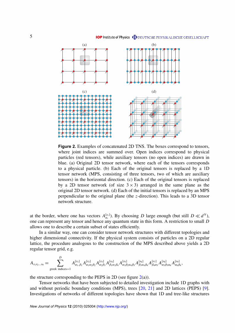
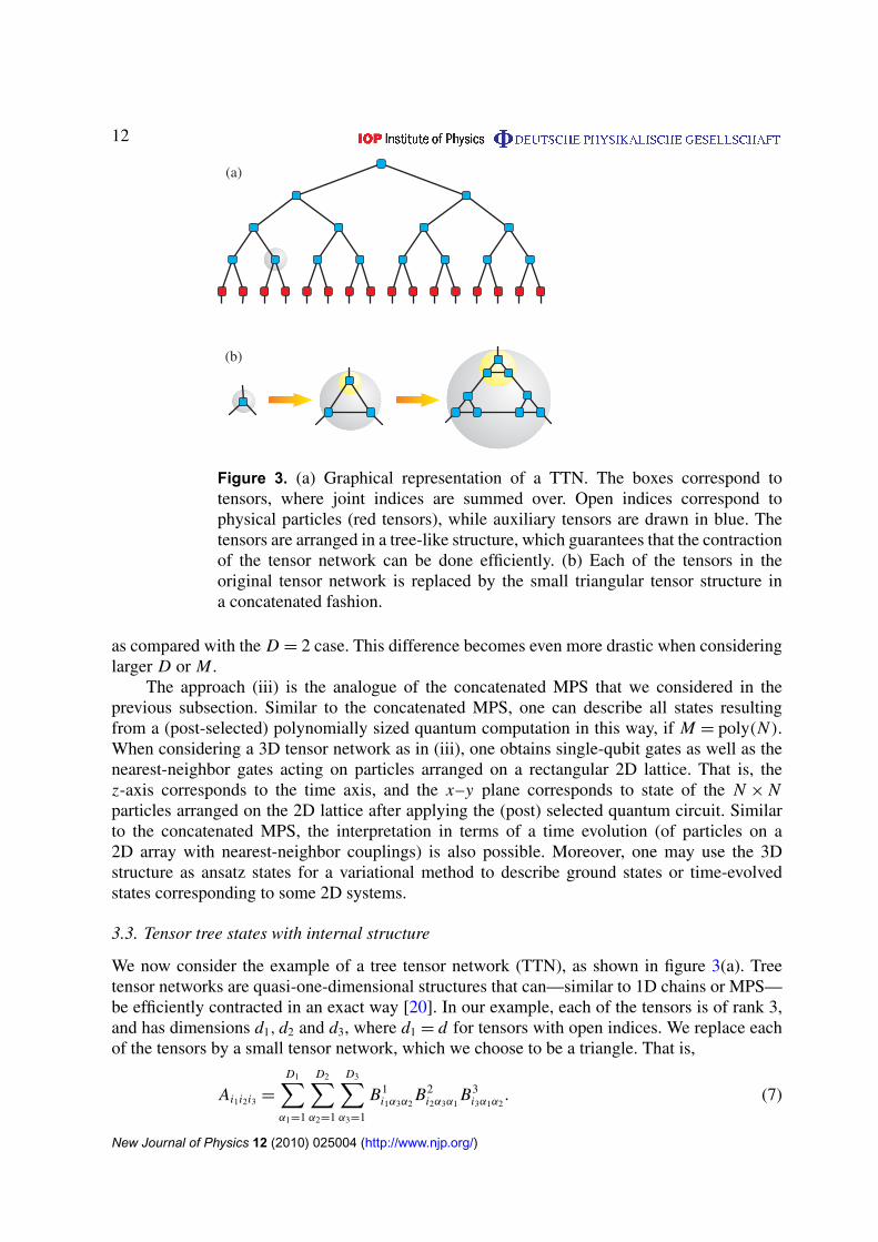
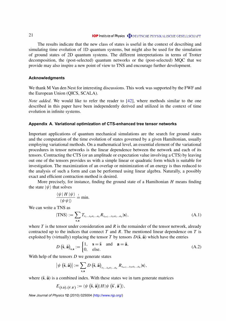
Figure 3. (a) Graphical representation of a TTN. The boxes correspond totensors, where joint indices are summed over. Open indices correspond tophysical particles (red tensors), while auxiliary tensors are drawn in blue. Thetensors are arranged in a tree-like structure, which guarantees that the contractionof the tensor network can be done efficiently. (b) Each of the tensors in theoriginal tensor network is replaced by the small triangular tensor structure ina concatenated fashion.

as compared with the D = 2 case. This difference becomes even more drastic when consideringlarger D or M .

The approach (iii) is the analogue of the concatenated MPS that we considered in theprevious subsection. Similar to the concatenated MPS, one can describe all states resultingfrom a (post-selected) polynomially sized quantum computation in this way, if M = poly(N ).When considering a 3D tensor network as in (iii), one obtains single-qubit gates as well as thenearest-neighbor gates acting on particles arranged on a rectangular 2D lattice. That is, thez-axis corresponds to the time axis, and the x–y plane corresponds to state of the N × Nparticles arranged on the 2D lattice after applying the (post) selected quantum circuit. Similarto the concatenated MPS, the interpretation in terms of a time evolution (of particles on a2D array with nearest-neighbor couplings) is also possible. Moreover, one may use the 3Dstructure as ansatz states for a variational method to describe ground states or time-evolvedstates corresponding to some 2D systems.

3.3. Tensor tree states with internal structure

We now consider the example of a tree tensor network (TTN), as shown in figure 3(a). Treetensor networks are quasi-one-dimensional structures that can—similar to 1D chains or MPS—be efficiently contracted in an exact way [20]. In our example, each of the tensors is of rank 3,and has dimensions d1, d2 and d3, where d1 = d for tensors with open indices. We replace eachof the tensors by a small tensor network, which we choose to be a triangle. That is,

Ai1i2i3 =

D1∑α1=1

D2∑α2=1

D3∑α3=1

B1i1α3α2

B2i2α3α1

B3i3α1α2

. (7)

New Journal of Physics 12 (2010) 025004 (http://www.njp.org/)

13

This process can now be iterated, i.e. each of the tensors Aii1αkαl

is replaced by three tensors,

say C i, jβ1β2β3

, in a triangular structure (see figure 3(b)). There are two different types of tensors:External tensors—i.e. ones that are connected to outside initial tensors—of dimensions di , D j

and Dk , respectively, and internal tensors that have dimensions Di , D j and Dk .We consider a situation where Di < d j . In such a case, the internal structure of the initial

tensor Ai1i2i3 is determined by elementary tensors C i, jβ1β2β3

, and in general this restricts thevalues of Ai1i2i3 . Note that the entanglement features of the corresponding CTS, as measuredby the entropy of entanglement, are determined by the dimensions of the tensors, and are inparticular limited by the dimension of the external links, i.e. d1, d2 and d3. That is, in termsof entanglement, nothing can be gained by introducing the internal tensor structure. In orderthat the resulting TNS can carry the same amount of entanglement as the one described bythe initial TTN, the dimension of inner links at concatenation level k needs to be are largerthan the square root of the dimension of the links at concatenation level k + 1. In particular,D1 >

√d1 for k = 1, while for k = 2 tensor dimension (for the inner links), D2 >

√D1 > d1/4

1are required. This can easily be seen by considering bipartitions of the system and by noting thatthe achievable Schmidt rank is determined by the dimension and the number of links betweenthe two groups.

The possible gain of such an internal tensor network structure is twofold. Firstly, thetotal number of parameters is reduced. While each initial tensor is described by d1d2d3

parameters, the resulting tensor network of depth k > 2 is described by (d1 + d2 + d3)D2 +3k−2 D3 parameters, where we assumed Dk = D for all internal links. Secondly, the size ofeach of the tensors in the internal tensor network structure is much smaller than the initialtensor. Many algorithms applied to the tensor network, e.g. the computation of normal formsof such tree tensor networks [20, 21, 37], or the optimization of tensors in a variationalmethod [38, 39], scale with the dimension of the elementary tensors of the network. In spite ofthe usually polynomial scaling of these algorithms, the computations quickly become intractablefor increasing dk , so that a network containing tensors with a small dimension are favorable ingeneral. We have utilized this approach in [38], where numerical simulations using tree tensornetworks are performed.

We remark that the contraction of the resulting tensor network becomes more difficultwhen compared to the initial tree structure. This is due to the fact that the concatenated tensornetwork contains loops. To retain numerical accessibility, either approximate treatments have tobe applied (as in contraction schemes introduced in the context of PEPS [19]) or the tree-likestructure has to be maintained, e.g. by limiting the tree width of the concatenated tensor network(as in [38]).

Tensor product states similar to the CTS are also considered in different contexts. Forexample, for the simulation of thermal states or higher dimensional classical spin models, a(variational) tensor product ansatz of this kind proved to be useful [40].

4. Applications

After having given some theoretical and analytical considerations for the possible advantagesof CTS over other numerical methods for the description of states, we want to demonstrateapplications of the CTS structure. The relevance of the CTS rests on two pillars. The first one isthe ability of the (concatenated) tensor network to actually hold the relevant information about

New Journal of Physics 12 (2010) 025004 (http://www.njp.org/)

14

a state. The analytical considerations above indicate that this is the case for states based oncircuits, time-evolved states and others. The second pillar is the question if we can, once givena CTS, read out the contained information. Progress has been made with very similar networksin the context of PEPS. What we want to demonstrate in the following is the ability to findthe potentially good description with numerically accessible methods and see how good theapproximation is. Moreover, this section aims to demonstrate the applicability of the knowncontraction methods and describe some improvements thereof.

4.1. The descriptive potential of CTS

In this section, we want to demonstrate the descriptive potential of a CTS using a toy model.For reasons of comparison, relevant states of the toy model were calculated exactly and theseexact states were then approximated with both MPS and CTS. To avoid infiltrating the CTSdescription with inaccuracies from an approximate read-out procedure, we used an exactcontraction algorithm for this network6.

In particular, we have tested the achievable accuracies when describing states resultingfrom time evolution in a spin chain, using the Hamiltonian

H =

∑a

σ (a)z σ (a+1)z + B

∑a

σ (a)x , (8)

with B = 1 and a system size of N = 12 physical sites. The system is initialized in the productstate |+〉

⊗N and has evolved over a time T = 3.5, a point which is, in our units, close to thepoint where the fidelity of the CTS had a (periodically recurring) minimum. Time evolutionunder this Hamiltonian shows the typical growth of entanglement in the state that makes MPS-based description difficult. The optimal tensors in the CTS and also the MPS description wereapproximated by optimizing the overlap of the exactly calculated state and the (TNS) in asweeping procedure. For each tensor, the overlap

|〈ψex|ψCTS〉|2

〈ψex|ψex〉〈ψCTS|ψCTS〉

was calculated, leaving out one tensor to optimize. This tensor can then be found using linearalgebra techniques using the contraction result as a linear form. See [9, 19] and appendix A.

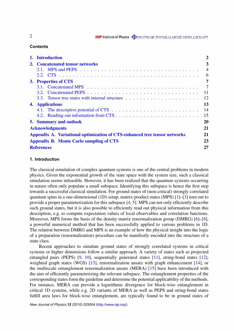
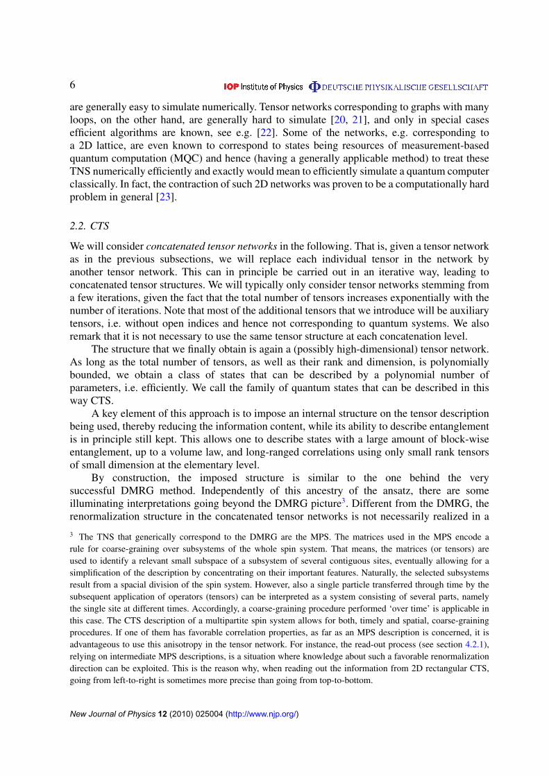
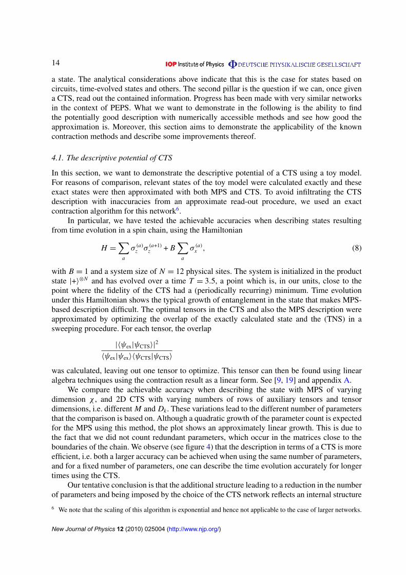
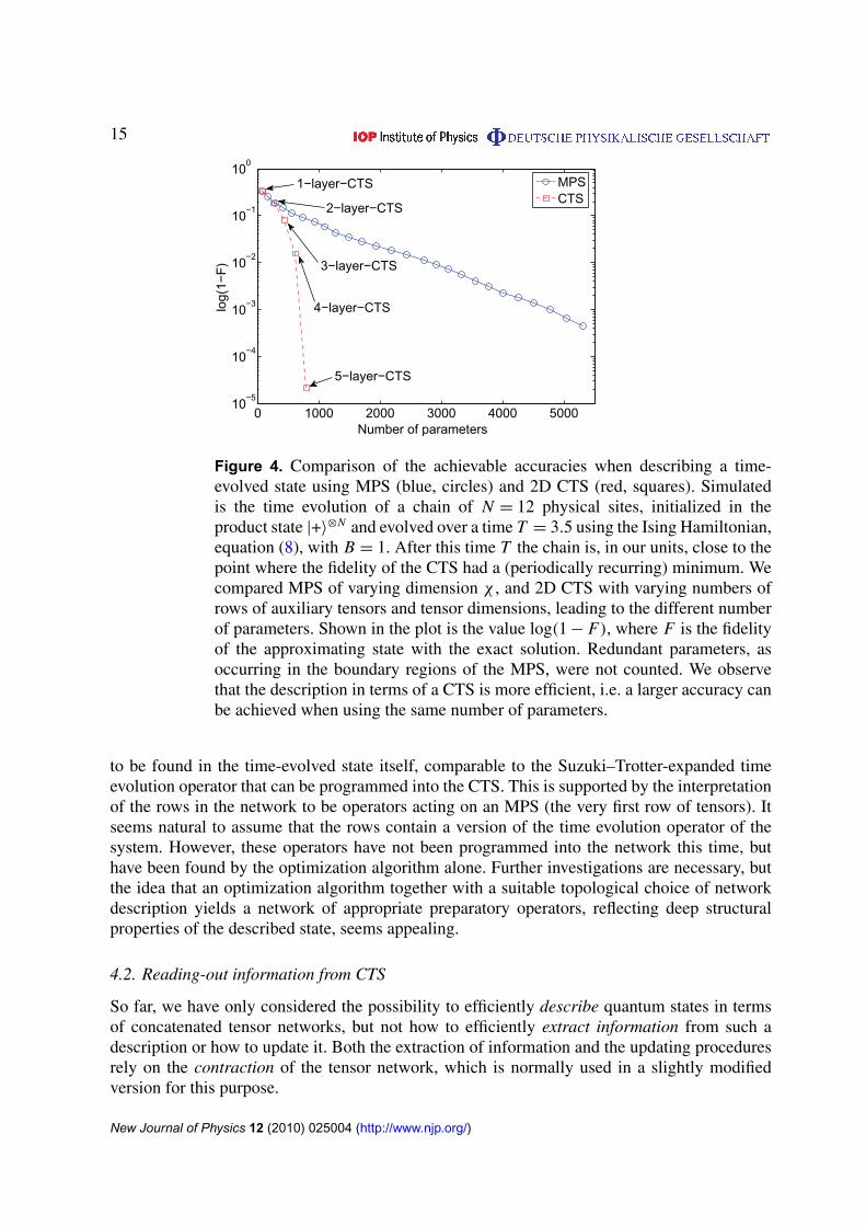
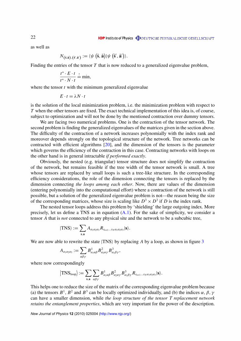
We compare the achievable accuracy when describing the state with MPS of varyingdimension χ , and 2D CTS with varying numbers of rows of auxiliary tensors and tensordimensions, i.e. different M and Dk . These variations lead to the different number of parametersthat the comparison is based on. Although a quadratic growth of the parameter count is expectedfor the MPS using this method, the plot shows an approximately linear growth. This is due tothe fact that we did not count redundant parameters, which occur in the matrices close to theboundaries of the chain. We observe (see figure 4) that the description in terms of a CTS is moreefficient, i.e. both a larger accuracy can be achieved when using the same number of parameters,and for a fixed number of parameters, one can describe the time evolution accurately for longertimes using the CTS.

Our tentative conclusion is that the additional structure leading to a reduction in the numberof parameters and being imposed by the choice of the CTS network reflects an internal structure

6 We note that the scaling of this algorithm is exponential and hence not applicable to the case of larger networks.

New Journal of Physics 12 (2010) 025004 (http://www.njp.org/)

15

0 1000 2000 3000 4000 500010

−5

10−4

10−3

10−2

10−1

100

log(

1−F

)

Number of parameters

MPSCTS

5−layer−CTS

4−layer−CTS

3−layer−CTS

1−layer−CTS

2−layer−CTS

Figure 4. Comparison of the achievable accuracies when describing a time-evolved state using MPS (blue, circles) and 2D CTS (red, squares). Simulatedis the time evolution of a chain of N = 12 physical sites, initialized in theproduct state |+〉

⊗N and evolved over a time T = 3.5 using the Ising Hamiltonian,equation (8), with B = 1. After this time T the chain is, in our units, close to thepoint where the fidelity of the CTS had a (periodically recurring) minimum. Wecompared MPS of varying dimension χ , and 2D CTS with varying numbers ofrows of auxiliary tensors and tensor dimensions, leading to the different numberof parameters. Shown in the plot is the value log(1 − F), where F is the fidelityof the approximating state with the exact solution. Redundant parameters, asoccurring in the boundary regions of the MPS, were not counted. We observethat the description in terms of a CTS is more efficient, i.e. a larger accuracy canbe achieved when using the same number of parameters.

to be found in the time-evolved state itself, comparable to the Suzuki–Trotter-expanded timeevolution operator that can be programmed into the CTS. This is supported by the interpretationof the rows in the network to be operators acting on an MPS (the very first row of tensors). Itseems natural to assume that the rows contain a version of the time evolution operator of thesystem. However, these operators have not been programmed into the network this time, buthave been found by the optimization algorithm alone. Further investigations are necessary, butthe idea that an optimization algorithm together with a suitable topological choice of networkdescription yields a network of appropriate preparatory operators, reflecting deep structuralproperties of the described state, seems appealing.

4.2. Reading-out information from CTS

So far, we have only considered the possibility to efficiently describe quantum states in termsof concatenated tensor networks, but not how to efficiently extract information from such adescription or how to update it. Both the extraction of information and the updating proceduresrely on the contraction of the tensor network, which is normally used in a slightly modifiedversion for this purpose.

New Journal of Physics 12 (2010) 025004 (http://www.njp.org/)

16

Given the fact that already a 2D tensor network is sufficient to describe all states resultingfrom a polynomial-sized quantum computation, one does not expect an efficient contractionof such a tensor network to be possible in general. In fact, it has been shown in [23] thatcontracting 2D tensor networks is computationally hard, and the corresponding complexityclass is #P . However, this does not mean that no efficient approximate methods can exist whichcan successfully be applied in practice. In fact, in [9] an approximate method to contract 2Dtensor networks has been introduced and successfully applied in, e.g. the context of a ground-state approximation for strongly correlated 2D systems [19]. This method will be described inthe following, together with an investigation of two additional techniques: (i) a novel error-correction scheme and (ii) an MPO-compression scheme.

For specific tensor network topologies (e.g. networks corresponding to 1D graphs, treesor networks with a bounded tree width [37]), an exact and efficient contraction and update oftensors is possible. If we are able to choose the contraction order of all indices, there exist MCbased methods for the contraction, whose application will be shown in appendix B.

4.2.1. Approximate contraction of 2D tensor networks. The approximate contraction of a 2Dtensor network with open boundary conditions, as introduced in [9], works as follows. The first(e.g. horizontal) line of tensors at the boundary can be interpreted as an MPS, where the lowerindices are considered as open. The second line can be viewed as an MPO acting on the firstmatrix product state. The resulting state (after contracting two lines) can again be described byan MPS, but of increased dimension. The aim is now to find (e.g. via a variational method)the optimal approximation of the resulting state by an MPS of fixed (low) dimension. This is,e.g. done by optimizing the individual tensors via solving a generalized eigenvalue problem(see [9] or appendix A below). The MPS found this way is now processed further, i.e. the MPOcorresponding to the third line of tensors is applied, and once again aims at obtaining a properapproximation of the resulting state by an MPS of fixed dimension. The process is repeated untilthe second to last line of tensors is reached. The final step corresponds to calculating the overlapof the MPS resulting from the above procedure (after processing all but the final line), and theMPS corresponding to the final line. All of these steps can be done efficiently. The evaluationof expectation values of (tensor product) observables works in a similar way. For details ofthe method, we refer the reader to [19]. Note that the same method can be used for 2D tensornetworks where some of the tensors are auxiliary tensors (without open indices), as we considerin this paper.

When using a concatenated MPS as described in section 3.1, one may use the approximatemethod described above. However, especially when considering the description of timeevolution (section 3.1.2) or (post-selected) quantum circuits (section 3.1.1), it is important toapply the method in a proper way, possibly utilizing symmetries of the state. In particular, inthese cases the contraction should be done in the direction perpendicular to the order of thephysical sites (left to right or right to left), rather than in lines parallel to the physical sites(up-down or down-up). A contraction in an up-down direction would in these cases actuallycorrespond to describing the state after each time step in terms of a fixed-sized MPS, and isactually equivalent to the time evolution of an MPS as considered, e.g. in [41]. When usinga contraction in the perpendicular direction, such a limitation does not apply, see also [42].Numerical evidence suggests a significant increase in accuracy in this case. Moreover, thetreatment of infinitely extended, translationally invariant states leads to the observation thata contraction over infinitely many columns of tensors perpendicular to the physical direction

New Journal of Physics 12 (2010) 025004 (http://www.njp.org/)

17

often results in a projection onto the eigenspace with the largest-magnitude eigenvalues of theMPO represented by the column. This makes it possible to employ additional exact numericaltechniques, see, e.g. [42].

If one is, like in the case of CTS, moreover able to choose the indices to contract freely,certain choices of tensors may allow for an efficient approximation via the Monte Carlo (MC)sampling techniques [43], see appendix B. There, the application of MC methods to a 2D CTSwill be demonstrated, using the inherent MPO structure of the CTS. We would also like tomention the possibility to utilize String-bond state like tensor networks [12] in the context ofCTS. Additionally, for certain choices of the tensors, it is known that an exact and efficientcontraction is possible [22].

In the following, we would like to suggest two improvements for the traditional contractionscheme.

4.2.2. An error-correction scheme. We will now describe an error-correcting procedure for thecontraction of the 2D CTS, which is applicable also to the contraction of other rectangular gridsincluding the PEPS.

We start with the traditional approximate contraction using the method described above,resulting in a number C , holding the contraction result. Following the line of argument from thesections above, we can interpret the number C as an approximation of the number

C = 〈M1|M2 · · · MN−1|MN 〉,

where 〈M1| is the MPS defined by the leftmost column of tensors, the operators Mi are the MPOdefined by the columns in the middle and |MN 〉 is the MPS defined by the rightmost columnof tensors in the CTS. To remind the reader, a left-to-right contraction of the CTS involves theiteration of the following steps: (i) start with i = 1 and set 〈M1| := 〈M1|. (ii) Apply the MPOMi+1 to the intermediate MPS 〈M1,...,i |. Both having a small bond-dimension, we obtain anMPS of a large bond-dimension, 〈M1,...,i+1|. (iii) Reduce the bond-dimension of 〈M1,...,i+1| toobtain another intermediate MPS 〈M1,...,i+1|, representing 〈M1,...,i+1| as good as possible withthis smaller bond-dimension. (iv) Increase i by one and continue with step (ii). The aim of theerror-correcting scheme is to estimate the error introduced by cutting off the bond-dimension ofthe intermediate MPS, and to correct the result C accordingly.

More precisely, after the (i − 1)th step of the standard left-to-right contraction, the CTS isapproximated by

C ≈ Ci−1 = 〈M1,...,i |Mi+1 · · · MN−1|MN 〉,

where 〈M1,...,i | ≈ 〈M1|M2 · · · Mi . In the i th step, we use the approximation 〈M1,...,i+1| ≈

〈M1,...,i |Mi+1 resulting in

C ≈ Ci = 〈M1,...,i+1|Mi+2 · · · MN−1|MN 〉.

The additional error of C in the i th approximation step is given by the value εi = Ci−1 − Ci , andthe optimally corrected value of the contraction result is given by

C = C +∑

i

εi . (9)

New Journal of Physics 12 (2010) 025004 (http://www.njp.org/)

18

However, usually neither Ci−1 nor Ci can be calculated exactly since the exact MPS descriptionof the state Mi+2 · · · MN−1|MN 〉 is too large to be computed. The crucial observation now is thatthe (N − i − 2)th step of a right-to-left contraction is a good approximation of this state with

|M i+2,...,N 〉 ≈ Mi+2 · · · MN−1|MN 〉,

which can be used to estimate the error εi produced by the i th step of the left-to-right contraction

εi = Ci−1 − Ci

≈ 〈M1,...,i |Mi+1|M i+2,...,N 〉 − 〈M1,...,i+1|M i+2,...,N 〉. (10)

This approximate value of εi is then used in equation (9).For an estimation of the achievable accuracy with this error-correction scheme, let the error

of the overall left-to-right contraction be ε. We note that the error of the right-to-left contractionand its intermediate results 〈M i,...,n| are also of this size. Since the magnitude of the differencein equation (10) is also of the order ε, we are left with a residual absolute error of the orderε2 after the error correction. An application to toy models has confirmed our error estimationand yields a reduction of the error of about one order of ε, or even better. For instance, theapproximate contraction of the time-evolved state in section 4.1 with a cut-off bond-dimensionD = 12 results in a value C with error correction an error of 1.6(7)% with error correction and25(10)% without error correction, taking the mean of several approximations.

While a similar reduction could in principle be achieved by using a bigger cut-off bond-dimension for the intermediate results, the error-correction scheme is favorable in most casesbecause of its better performance. As we can obtain all the required states 〈M i,...,n| by cachingone right-to-left contraction, we need merely twice the computation time for reducing the errorby a factor of ε. The overhead in memory depends on the cut-off bond-dimension of the states〈M i,...,n|. Choosing this dimension as equal to the dimension of the MPO Mi , the overheadis less than a factor of two, as we have to store N − 3 extra MPS, which is less than the(N − 2)MPO + 2MPS of the CTS.

We remark that the applicability of this error-correction scheme is not restricted to the CTS,but can in a similar way also be used, e.g. in the context of the 2D PEPS approach.

4.2.3. Compressibility of sequences of MPO. Additionally, the number of tensors in theCTS description can be reduced significantly below the number needed in the canonicalimplementation of the Suzuki–Trotter picture, as given in section 3.1.2, or for a generic networkof (sparse) operators, like circuits.

The reason for this is that it is not necessary to restrict each row to the description ofa single Suzuki–Trotter (or generic operator circuit) time step only. Instead we can first puta good approximation for many of these rows, applied successively, into one row, thus usingthe descriptive power of the CTS to the maximal extent. This is possible by calculating andoptimizing the overlap of one row of (variable) tensors with several concatenated rows of fixedtensors, in a way similar to maximizing the norm of a CTS when keeping every row but onefixed. We then concatenate these optimal rows, being fewer apparently, to reduce computationaltime in the read-out process, whose computation time relies on the number of tensors involved.

To get an idea of the potential of this ansatz, let us consider time evolution. Whenperforming time evolution by a Suzuki–Trotter expansion with an MPO compression, there aretwo possible sources of error. The first kind of errors comes from the MPO approximation. Thiskind of error can be controlled, as we know the fidelity of the replacement step (the overlap

New Journal of Physics 12 (2010) 025004 (http://www.njp.org/)

19

of the rows to be compressed with the replacement row). When this fidelity is too small, wecan reduce the number of rows to be compressed. The second kind of error comes from theSuzuki–Trotter expansion itself. This error can be made small by choosing a very small timestep, so that the MPO corresponding to one row is close to unity. After compressing two rowsto one, we are able to iterate the compression and compress two already compressed rows toone row, which now represents four time steps. This way, we obtain one operator covering 2n

time steps with only n compression steps. Taking initially very small time steps thus does notresult in a big performance hit, as the compression is very strong here, i.e. it is exponential, andcompensates for it. The compression can of course only be applied as long as one row can inprinciple hold the whole time step, but the results from the toy model in section 4.1 make usoptimistic that a row has the potential to hold comparatively big time steps. Numerical evidenceconcerning the compression fidelity for a variety of operators supports this view. In this case,the compression not only improves the computation time but also the achievable precision byreducing the error introduced by Trotterization.

The variational ansatz just shown leads to a picture of the CTS where a fixed number oftensors will be employed in an optimal way, as opposed to the direct programming of a set ofanalytically accessible operators into the network.

4.2.4. Special cases—exact contraction. Even though the problem of contracting an arbitrary2D tensor network is in general computationally difficult (#P hard), under certain conditions, anefficient and exact contraction of certain networks is possible.

One such example are planar tensor networks, where each of the tensors fulfills a so-called match-gate (or free fermion) condition [22]. It follows that if we restrict ourselves toCTS corresponding to planar structures, one can calculate the norm as well as the expectationvalues of the tensor product of observables efficiently for such states, as long as all tensors inthe tensor network fulfill the match-gate condition. This implies that one may use such CTS,e.g. as variational ansatz states for ground states or time evolution. In particular, we point outthat the usage of auxiliary tensors as we propose for 2D CTS can be handled in exactly the samefashion.

Another example are networks corresponding to trees or structures with a bounded or onlylogarithmically growing tree width. These also can be contracted efficiently and exactly. Forinstance, the contraction of a subcubic tensor tree (i.e. a tensor network where each of thetensors in the tree is connected with three or less neighbors) has a computational effort scalingas O(D3). For a variational method for the search for ground states and the maximization ofoverlaps with CTS-enhanced TTN, see appendix A.

4.2.5. The advantage of CTS in the operator picture. Being able to program the Suzuki–Trotter expanded time evolution operator or other generic quantum circuits directly into thestate description offers access to alternative advantageous numerical approaches. Time evolutionmethods usually rely on maximizing a significant number of overlaps of the kind

|〈ψt+δt |τ(δt)|ψt〉|2

〈ψt+δt |ψt+δt〉〈ψt |ψt〉,

where τ(δt) is the time evolution operator for a time δt , |ψt〉 is a known TNS and the tensorsdescribing the state |ψt+δt〉 have to be found. In the context of circuits, an application of a setof gates can be regarded as a time step like above. Starting from this expression, to compute

New Journal of Physics 12 (2010) 025004 (http://www.njp.org/)

20

the time-evolved state after a time T , one would have to compute single time steps repeatedly,and each time one would have to perform network contractions to determine the optimal tensorentries. (Algorithms of this kind are found to converge to a reasonable approximation of thebest tensor network description of the desired time-evolved state |ψT〉.) Depending on theimplementation, finding the optimal tensors can consist of many substeps, e.g. a sweepingprocedure approximating single tensors while leaving the remaining tensors fixed, each substeprequiring another contraction.

The CTS description of states is very efficient in this regard if, as given above, the timeevolution operator τ(T )=

∏τ(δt) is programmed into the structure and description of the state

itself. Using CTS, we are able to circumvent the many contractions and possible sweeping stepsby a single optimized contraction. In contrast to a traditional MPS time evolution, for example,it is possible to use error-correction and alternative contraction order (e.g. left-to-right insteadof top-to-bottom). Moreover, we are able to employ MPO compression, which is, however, alsoapplicable to the traditional time evolution method, but not in a direction-optimized fashion.

5. Summary and outlook

We have introduced CTS, a class of states that is obtained by decomposing the high-ranktensor describing the coefficients of multiparticle states into a tensor network in an iterativefashion. The basic idea is to impose an additional structure to each of the tensors appearing in atensor network description of a given state. We have demonstrated this approach for 1D tensornetworks, where in the first step, a description in terms of a matrix product state is obtained.Each of the matrices (tensors) is then further decomposed into a 1D tensor network (MPO),yielding a 2D tensor network with many auxiliary tensors in the next step. Similar methods canbe applied to 2D systems, yielding 2D or 3D PEPS with auxiliary tensors, or to TTN.

We have demonstrated that with such CTS, one can describe multiparticle quantum systemswith rich entanglement features in an efficient way. In particular, states arising from timeevolution or generated by polynomial (post-selected) quantum circuits can be described, andan interpretation in terms of (post-selected) measurement-based quantum computation can begiven. The states can—in contrast to MPS or PEPS—contain a large amount of blockwiseentanglement (up to a volume law) and long-ranged correlations, while their description remainsefficient. In particular, a subclass of MPS and PEPS with a high-effective bond dimension canbe described.

We have demonstrated that it is possible to describe states arising from time evolution ofa 1D quantum system with help of such a 2D CTS more efficiently than with a matrix productstate. We have discussed the description arising from a Trotter decomposition of the evolutionoperator, as well as direct optimization of (auxiliary) tensors in the 2D tensor network of givensize and dimension. In this context, we have also applied a method to compress MPO to obtaina more efficient description of the time-evolved state.

We have also discussed and improved methods to read out information from 2D tensornetworks. The applicability of approximate contraction methods, possibly with differentdirections of contraction (left-to-right), has been discussed and improved using an error-correction scheme. Both the effectiveness of the CTS description in the context of time evolutionof 1D systems as well as the impact of our suggested enhancements to the traditional read-outmethods were demonstrated using numerical results for a toy model. Also the applicability ofMC methods for the contraction was demonstrated.

New Journal of Physics 12 (2010) 025004 (http://www.njp.org/)

21

The results indicate that the new class of states is useful in the context of describing andsimulating time evolution of 1D quantum systems, but might also be used for the simulationof ground states of 2D quantum systems. The different interpretations in terms of Trotterdecomposition, the (post-selected) quantum networks or the (post-selected) MQC that weprovide may also inspire a new point of view to TNS and encourage further development.

Acknowledgments

We thank M Van den Nest for interesting discussions. This work was supported by the FWF andthe European Union (QICS, SCALA).

Note added. We would like to refer the reader to [42], where methods similar to the onedescribed in this paper have been independently derived and utilized in the context of timeevolution in infinite systems.

Appendix A. Variational optimization of CTS-enhanced tree tensor networks

Important applications of quantum mechanical simulations are the search for ground statesand the computation of the time evolution of states governed by a given Hamiltonian, usuallyemploying variational methods. On a mathematical level, an essential element of the variationalprocedures in tensor networks is the linear dependence between the network and each of itstensors. Contracting the CTS (or an amplitude or expectation value involving a CTS) by leavingout one of the tensors provides us with a simple linear or quadratic form which is suitable forinvestigation. The maximization of an overlap or minimization of an energy is thus reduced tothe analysis of such a form and can be performed using linear algebra. Naturally, a possiblyexact and efficient contraction method is desired.

More precisely, for instance, finding the ground state of a Hamiltonian H means findingthe state |ψ〉 that solves

〈ψ | H |ψ〉

〈ψψ |〉

!= min.

We can write a TNS as

|TNS〉 :=∑s,a

Ts1...sna1...an Rsn+1...sN a1...an |s〉, (A.1)

where T is the tensor under consideration and R is the remainder of the tensor network, alreadycontracted up to the indices that connect T and R. The mentioned linear dependence on T isexploited by (virtually) replacing the tensor T by tensors D(s, a) which have the entries

D(s, a

)s,a :=

{1, s = s and a = a,0, else.

(A.2)

With help of the tensors D we generate states∣∣ψ (s, a)⟩

:=∑s,a

D(s, a

)s1...sna1...an

Rsn+1...sN a1...an |s〉,

where (s, a) is a combined index. With these states we in turn generate matrices

E(s,a),(s′,a′) := 〈ψ(s, a

)|H |ψ

(s′, a′

)〉,

New Journal of Physics 12 (2010) 025004 (http://www.njp.org/)

22

as well as

N(s,a),(s′,a′) := 〈ψ(s, a

)|ψ(s′, a′

)〉.

Finding the entries of the tensor T that is now reduced to a generalized eigenvalue problem,

t∗· E · t

t∗ · N · t!= min,

where the tensor t with the minimum generalized eigenvalue

E · t = λN · t

is the solution of the local minimization problem, i.e. the minimization problem with respect toT when the other tensors are fixed. The exact technical implementation of this idea is, of course,subject to optimization and will not be done by the mentioned contraction over dummy tensors.

We are facing two numerical problems. One is the contraction of the tensor network. Thesecond problem is finding the generalized eigenvalues of the matrices given in the section above.The difficulty of the contraction of a network increases polynomially with the index rank andmoreover depends strongly on the topological structure of the network. Tree networks can becontracted with efficient algorithms [20], and the dimension of the tensors is the parameterwhich governs the efficiency of the contraction in this case. Contracting networks with loops onthe other hand is in general intractable if performed exactly.

Obviously, the nested (e.g. triangular) tensor structure does not simplify the contractionof the network, but remains feasible if the tree width of the tensor network is small. A treewhose tensors are replaced by small loops is such a tree-like structure. In the correspondingefficiency considerations, the role of the dimension connecting the tensors is replaced by thedimension connecting the loops among each other. Now, there are values of the dimension(entering polynomially into the computational effort) where a contraction of the network is stillpossible, but a solution of the generalized eigenvalue problem is not—the reason being the sizeof the corresponding matrices, whose size is scaling like D3

× D3 if D is the index rank.The nested tensor loops address this problem by ‘shielding’ the large outgoing index. More

precisely, let us define a TNS as in equation (A.1). For the sake of simplicity, we consider atensor A that is not connected to any physical site and the network to be a subcubic tree,

|TNS〉 :=∑s,a

Aa1a2a3 Rsn+1...sN a1a2a3|s〉.

We are now able to rewrite the state |TNS〉 by replacing A by a loop, as shown in figure 3

Aa1a2a3 :=∑αβγ

B1a1αβ

B2a2αγ

B3a3βγ

,

where now correspondingly∣∣TNSloop

⟩:=∑s,a

∑αβγ

B1a1αβ

B2a2αγ

B3a3βγ

Rsn+1...sN a1a2a3|s〉.

This helps one to reduce the size of the matrix of the corresponding eigenvalue problem because(a) the tensors B1, B2 and B3 can be locally optimized individually, and (b) the indices α, β, γcan have a smaller dimension, while the loop structure of the tensor T replacement networkretains the entanglement properties, which are very important for the power of the description.

New Journal of Physics 12 (2010) 025004 (http://www.njp.org/)

23

It is possible to choose low but sufficiently high index rank for the internal indices such that theentanglement being carried by the external indices (that connect the loops among each other) isnot reduced.

In detail, finding the optimal values of the loop tensors B i can be performed as follows.First, the network represented by R has to be contracted. Once this tensor is found, it is keptfixed for the optimization of the tensors B i . We then repeat the optimization steps for the looptensors as described in the section above, using the state

∣∣TNSloop

⟩:=∑s,a

∑αβγ

d1(

a1, α, β)

a1αβB2

a2αγB3

a3βγRsn+1...sN a1a2a3 |s〉 ,

with a tensor d1 like in equation (A.2). Similarly, we proceed for the tensors B2 and B3. In thesesteps we can make use of the fact that several (more than one) sweeps through the loop tensorswill give a better convergence, while the computational overhead for this is small, because thehuge remainder of the network—represented by the tensor R—stays constant and does not needto be contracted again. If the dimension of the internal indices is large enough, several sweepsthrough the loop will converge to a network

Aa1a2a3 :=∑αβγ

B1a1αβ

B2a2αγ

B3a3βγ

,

with a tensor A whose values are the same as in the case without the replacement network. Insome cases, the original problem of finding A would not have been feasible, but even if it is so,the sweeping through the loop gives an advantage in computation time.

Appendix B. Monte Carlo sampling of CTS

In some instances, it is possible to contract the concatenated tensor network approximately withan MC-based approach. For this, let us quickly recall how the MC method works. The easiestand most basic MC technique is the Metropolis algorithm [44]. Like all MC methods, it is usedto estimate integrals (or sums) over high dimensional integration spaces. In these spaces, naïveapproaches like Riemann-integration require a huge number of sampling points for a certainrequired accuracy, whereas usually the MC methods show a much quicker convergence to theexact value.

The basic idea is that we can select a sample of points in the integration space such that

Z−1

∫V

f (x)µ(x)dx ≈ N−1∑

{xi }Ni=1⊂V

f (xi)4v,

where Mv is a unit volume in V , µ is a well-behaved measure on V and Z =∫

V µ(x)dx .Naturally, the selection rule for the set of samples, {xi}, is the key and has a foundation instatistical mechanics. Assume that f is a property of an ergodic physical system with density(probability density to be found at that point) µ in a configuration space. The system beingergodic, we know that the time average of the property f equals the average of f over theconfiguration space with weight µ,

〈 f 〉t =

∫V

f (x)µ(x)dx .

New Journal of Physics 12 (2010) 025004 (http://www.njp.org/)

24

We obtain the set of samples {xi} by simulating the behavior of the system in time and recordingthe position x(ti)= xi at discretely (and equally) spaced points {ti} in time. Now let P(x → x ′)

be the probability of the system to go, during one discrete time step of a random walk, frompoint x to point x ′. A set {xi} of a random walk derived with such a rule is called a Markovchain, with the essential property being that xi is only dependent on xi−1 (and not on xi−2 etc).It is known that the so-called detailed balance condition for the probability P ,

µ(x)P(x → x ′)= µ(x ′)P(x ′→ x),

is a sufficient criterion to ensure that a random walk of the system, ruled by the transferprobability P , yields a time average approaching the value Z−1

∫V f (x)µ(x)dx for t → ∞.

One can impose this transfer probability by the following rule:

1. Being at point xi , choose randomly a position ξ .

2. Calculate the value A(xi → ξ)= min(1, µ(ξ)µ(xi )

).

3. Randomize a number in the interval a ∈ [0, 1].

4. If a < A(xi → ξ), then xi+1 = ξ ; otherwise xi+1 = xi .

This is the (basic) Metropolis algorithm [44]. The probability of going from x to x ′

under this algorithm obeys the detailed balance condition and hence yields a sample that isrepresentative for the measure µ. We note that with this rule we can generate arbitrarily largesets of positions in time without the need to store the set {xi} itself. Furthermore, it is notnecessary (for the evaluation of the time evolution) to know the value Z =

∫V µ(x)dx , which

cancels in the calculation of A; a fact that makes it possible to work with relative probabilitiesand unnormalized measures.

We now want to show that the contraction of the concatenated tensor networks canbe implemented via an MC algorithm. To demonstrate this principle, we give the formulaeto contract a toroidal network of N × M tensors of rank four, although the formalism iseasily adapted to non-toroidal networks and higher dimensions. Consequently, we want tocalculate ∑

indices su,sd,sl,sr

∏i, j

T i, jsu(i, j)sd(i, j)sl(i, j)sr(i, j),

where u, d, l, r mean ‘up, down, left, right’, respectively, the indices su,d,l,r depend on the position(i, j) within the network, and sd(i, j)= su(i + 1, j), sr(i, j)= sl(i, j + 1), su(1, j)= sd(N , j)and sl(i, 1)= sr(i, N ).

The basic principle is to perform the contraction over the indices su,d,l,r in a hierarchicalorder: we first contract over the indices in each row. This is formally the trace over a productof matrices, the matrices being the tensors of rank four, where the indices connecting in thevertical direction are kept fixed. In the next step, we contract over the indices that connectthe rows. Following this idea, in the case of an n-dimensional network, the hierarchy has nlevels—indices of increasing level thereby connecting slices of increasing dimensionality. Forthe problem at hand, we write∑

su,sl

∏i, j

T i, jsu(i, j)su(i+1, j)sl(i, j)sl(i, j+1) =

∑su

∏i

Risu(i)su(i+1), (B.1)

New Journal of Physics 12 (2010) 025004 (http://www.njp.org/)

25

where su(i)= (su(i, 1), su(i, 2), . . .),∏i

Risu(i)su(i+1) :=

∑sl

∏j

T i, jsu(i, j)su(i+1, j)sl(i, j)sl(i, j+1)

= Tr

∏j

T i, j [su (i, j) , su (i + 1, j)]

,and where T i, j [·, ··] are matrices with elements(

T i, j [a, b])

c,d:= T i, j

a,b,c,d .

What we see is that, while keeping the up and down indices fixed in each row, we obtain aset of matrices for each row, and carry out the summation of the left and right indices withmatrix products and a trace. As seen in equation (B.1), this leaves us with another set ofmatrices, Ri

su(i)su(i+1), which are treated like the matrices T i, j [·, ··]: they are multiplied and theproduct is traced over. This means that the contraction over the whole set of indices is the traceover a matrix product for matrices whose elements are again traces over matrix products. Thisrecursion repeats itself and adds another ‘generation’ of matrix products for every dimension ofthe tensor network to be contracted. If the tensor network was no torus, the boundaries wouldhave been taken by tensors of lower rank. This would then replace the trace by the contractionwith the tensor at the boundary; the situation is similar to MPS with periodic versus openboundary conditions.

As we see, formally, we use matrix products and traces over all levels of matrices inthe hierarchy, but for the second generation of matrix products and higher ones this cannotbe carried out explicitly anymore. While the dimensions of the T i, j [·, ··] matrices depend onour arbitrary choice of the index rank of the tensors T only—making the first generation ofmatrix products feasible—the dimensions of the second generation of matrices (here the rowmatrices R) is already much too large: the number of columns enters exponentially. This is thepoint where the MC sampling is used. We sample the (second and higher) generation of matrixproducts.

To improve readability, we leave out the index u from now on and write the matrix elementsin the following way Ri

su(i)su(i+1) = 〈si |Ri|si+1〉 (as usual in quantum mechanics). There are in

principle two possible ways to perform the MC-approach in detail.In the first, the contraction takes the form∑

s

∏i

Ris(i)s(i+1) =

∑s1,...,sN+1

〈s1|R1|s2〉〈s2|R

2. . .Rn|sn+1〉〈sn+1|R

n+1|sn+2〉〈sn+2|R

n+2. . .RN|sN+1〉

=

∑s1,...,sN+1

L(s1, . . ., sN+1)R(s1, . . ., sN+1)

=

∑s1,...,sN+1

|L(s1, . . ., sn+1)|2 R(sn+1, . . ., sN+1)

L(s1, . . ., sn+1)∗

=

∑s1,...,sN+1

µ(s1, . . ., sn+1) f (s1, . . ., sN+1), (B.2)

New Journal of Physics 12 (2010) 025004 (http://www.njp.org/)

26

whereL(s1, . . ., sn+1) := 〈s1|R1

|s2〉〈s2|R2. . .Rn|sn+1〉,

R(sn+1, . . ., sN+1) := 〈sn+1|Rn+1|sn+2〉〈sn+2|Rn+2. . .RN

|sN+1〉.

Here, L and µ are actually independent of sk, k > n + 2 and R is independent of sk, k < n. Thisway, we have derived a formal expression that is compatible with an MC approach: µ is apositive measure (obviously, µ> 0), f is a function to be integrated over and weighed by µ.The integration (summation) space is the set of all vectors S = (s1, . . . , sN+1).

The second, alternative, implementation of the MC approach is similar, but divides theintegration space into smaller subsections. We use the same ansatz, but this time, we do notlook at the functions L and R, but at the functions l and r :

l(s1, sn+1) :=∑

s2,...,sn

L(s1, . . . , sn+1),

r(sn+1, sN+1) :=∑

sn+2,...,sN

R(sn+1, . . . , sN+1),

instead. Then, ∑s

∏i

Ris(i)s(i+1) =

∑s1,sn+1,sN+1

|l(s1, sn+1)|2 r(sn+1, sN+1)

l(s1, sn+1)∗,

where the sum is performed over only three (instead of N + 1) vectors. The functions l and r ,which are sums themselves, can be calculated, again, with an MC approach. The expression

l(s1, sn+1)=

∑s2,...,sn

〈s1|R1|s2〉〈s2|R

2. . .Rn|sn+1〉

(and likewise r ) are very similar formally to the original expression for the whole sum inequation (B.2) and can be treated in an analogous fashion: another subdivision of the summationspace {s2, . . . , sn} into two parts will be initiated. This recursion will have a depth of orderlog(N ); hence, assuming we need for a summation over three vectors O(m) MC samples, thismethod will lead to a computational effort of O((2m)log N )= O(2log N N log m). The decision tochoose way 1 or way 2 should be based on tests concerning the achieved convergence speed anddepend on the problem at hand.

There is one more bookkeeping issue to consider in both the approaches. Let S[·] denotethe limes of the MC sampling over a Markov chain {Si}, approaching infinite length, that isgenerated by the measure µ. Then(∑

all S

µ(S)

)S[ f ] =

∑all S

µ(S) f (S),

that is, the MC summation yields a result as if the measure was normalized. Hence we need anestimate for the partition sum Z =

∑all S µ(S). It can be obtained through the relationship

S[µ−1] = Z−1∑all S

µ(S)µ−1(S)= Z−1|{S}|;

hence, Z = |{S}|(S[µ−1])−1. This doubles the computational effort.

New Journal of Physics 12 (2010) 025004 (http://www.njp.org/)

27

The applicability of the MC method is not universal, however, the limits being set by themeasure µ and the function f . As mentioned in the description of the MC method, the systemneeds to be ergodic. This is not the case if the measure µ has regions whose borders cannotbe crossed during a random walk. This phenomenon is usually due to the measure being zero(or very small compared to other regions) in some regions of the configuration space. In thiscase, the random walker decides too often to stay where it is and traverses the configurationspace either too slowly or not at all, obviously not yielding an interesting sample collection. Aproperty that can cause non-ergodicity is hence sparseness of the tensors in the concatenatedtensor network. A remedy for this problem is a local change of basis, and hence is readilyavailable.

Another, more serious, problem is the non-convergence of the MC sampling due to the so-called sign problem. This means that the relative error of the sampling method stays big over anexponentially large sampling set, because, roughly speaking, in the summation process two verybig sub-summands (with small relative error) cancel each other. This problem does not occur ifall (row-)tensor elements are > 0.

Also, other tensor structures are known to be accessible in similar ways. For instance, so-called string-bond states [12] can be efficiently contracted via the MC sampling. While in theinitial work only the string-bond states where all tensors are associated with physical particleshave been considered, one can easily adopt the construction of CTS states to string-bond states.In particular, one can use exactly the same tensor structures as for string-bond states, wherehowever only some of the tensors correspond to physical particles, while the other tensors areauxiliary.

We have performed numerical tests on this method and found that for certain cases oftensor networks, e.g. with positive tensor entries, the algorithm converges quickly to a value ofthe contraction result with a quickly decreasing relative error.

References

[1] Fannes M, Nachtergaele D and Werner R F 1992 Commun. Math. Phys. 144 443[2] Affleck I, Kennedy T, Lieb E H and Takesaki H 1988 Commun. Math. Phys. 115 477[3] Verstraete F, Porras D and Cirac J I 2004 Phys. Rev. Lett. 93 227205

Schuch N, Cirac I and Verstraete F 2008 Phys. Rev. Lett. 100 250501[4] Hastings M B 2007 J. Stat. Mech. P08024

Hastings M B 2007 Phys. Rev. B 76 035114[5] Verstraete F and Cirac J I 2006 Phys. Rev. B 73 094423[6] White S R 1992 Phys. Rev. Lett. 69 2863

White S R 1993 Phys. Rev. B 48 10345[7] Schollwöck U 2005 Rev. Mod. Phys. 77 259[8] Rommer S and Ostlund S 1997 Phys. Rev. B 55 2164[9] Verstraete F and Cirac J I 2004 arXiv:cond-mat/0407066

[10] Verstraete F, Wolf M M, Perez-Garcia D and Cirac J I 2006 Phys. Rev. Lett. 96 220601Perez-Garcia D, Verstraete F, Cirac J I and Wolf M M 2008 Quantum. Inf. Comput. 8 0650

[11] Bañuls M-C, Perez-Garcia D, Wolf M M, Verstraete F and Cirac J I 2008 Phys. Rev. A 77 052306[12] Schuch N, Wolf M M, Verstraete F and Cirac J I 2008 Phys. Rev. Lett. 100 040501[13] Anders S, Plenio M B, Dür W, Verstraete F and Briegel H J 2006 Phys. Rev. Lett. 97 107206

Anders S, Briegel H J and Dür W 2007 New J. Phys. 9 361

New Journal of Physics 12 (2010) 025004 (http://www.njp.org/)

28

[14] Hübener R, Kruszynska C, Hartmann L, Dür W, Verstraete F, Eisert J and Plenio M B 2009 Phys. Rev. A 79022317

[15] Vidal G 2007 Phys. Rev. Lett. 99 220405Rizzi M and Montangero S 2008 Phys. Rev. A 77 052328Vidal G 2008 Phys. Rev. Lett. 101 110501

[16] Schuch N, Wolf M, Vollbrecht K G H and Cirac J I 2008 New J. Phys. 10 033032[17] Calabrese P and Cardy J 2005 J. Stat. Mech. 0504 P010[18] Barahona F 1982 J. Phys. A: Math. Gen. 15 3241[19] Murg V, Verstraete F and Cirac J I 2007 Phys. Rev. A 75 033605[20] Shi Y, Duan L and Vidal G 2006 Phys. Rev. A 74 022320[21] Markov I and Shi Y-Y 2008 SIAM J. Comput. 38 963[22] Valiant L 2002 SIAM J. Comput. 31 1229

Knill E 2001 arXiv:quant-ph/0108033Terhal B M and DiVincenzo D P 2002 Phys. Rev. A 65 032325DiVincenzo D P and Terhal B M 2005 Found. Phys. 35 1967Bravyi S 2005 Quantum Inf. Comput. 5 216Bravyi S 2009 Contemp. Math. 482 179–211Bravyi S and Kitaev A 2002 Ann. Phys. 298 210

[23] Schuch N, Wolf M, Verstraete F and Cirac J I 2007 Phys. Rev. Lett. 98 140506[24] Murg V, Cirac J I, Pirvu B and Verstraete F 2008 arXiv:0804.3976[25] Dür W and Cirac J I 2002 Quantum Inf. Comput. 2 240[26] Oliveira R, Dahlsten O C O and Plenio M B 2007 Phys. Rev. Lett. 98 130502

Douglas A, Plato K, Dahlsten O C and Plenio M B 2008 Phys. Rev. A 78 042332[27] Znidaric M 2008 Phys. Rev. A 78 032324[28] Aaronson S complexity zoo[29] Van den Nest M, Dür W, Raussendorf R and Briegel H J 2008 arXiv:0805.1214[30] Vidal G 2003 Phys. Rev. Lett. 91 147902

Vidal G 2004 Phys. Rev. Lett. 93 040502[31] Jane E, Vidal G, Dür W, Zoller P and Cirac J I 2003 Quantum Inf. Comput. 3 15[32] Sornborger A T and Steward E D 1999 Phys. Rev. A 60 1956[33] Raussendorf R and Briegel H J 2001 Phys. Rev. Lett. 86 910[34] Raussendorf R and Briegel H J 2001 Phys. Rev. Lett. 86 5188[35] Mora C, Piani M, Dür W, Van den Nest M, Miyake A and Briegel H J in preparation[36] Van den Nest M, Miyake A, Dür W and Briegel H J 2006 Phys. Rev. Lett. 97 150504

Van den Nest M, Dür W, Miyake A and Briegel H J 2007 New J. Phys. 9 204[37] Van den Nest M, Dür W, Vidal G and Briegel H J 2007 Phys. Rev. A 75 012337[38] Hübener R, Kruszynska C, Hartmann L, Dür W, Verstraete F, Eisert J and Plenio M B in preparation[39] Tagliacozzo L, Evenbly G and Vidal G 2009 arXiv:0903.5017[40] Gendiar A, Maeshima N and Nishino T 2003 Prog. Theor. Phys. 110 691–9

Maeshima N, Hieida Y, Akutsu Y, Nishino T and Okunishi K 2001 Phys. Rev. E 64 016705Nishino T, Hieida Y, Okunishi K, Maeshima N and Akutsu Y 2001 Prog. Theor. Phys. 105 409–17Nishino T, Okunishi K, Hieida Y, Maeshima N and Akutsu Y 2000 Nucl. Phys. B 575 504–12

[41] Daley A J, Kollath C, Schollwoeck U and Vidal G 2004 J. Stat. Mech.: Theor. Exp. P04005[42] Bañuls M-C, Hastings M B, Verstraete F and Cirac J I 2009 Phys. Rev. Lett. 102 240603[43] Sandvik A W and Vidal G 2007 Phys. Rev. Lett. 99 220602[44] Metropolis N, Rosenbluth A W, Rosenbluth M N, Teller A H and Teller E 1953 J. Chem. Phys. 21 1087

New Journal of Physics 12 (2010) 025004 (http://www.njp.org/)