March 2011

Enquiries should be addressed to:Alex WonhasCSIRO Energy Transformed FlagshipPhone: +61- 2-9490-5059Email: alex.wonhas@csiro.au

Copyright and Dis claimer© 2011 CSIRO To the extent permitted by law, all rights are reserved and no part ofthis publication covered by copyright may be reproduced or copied in any form or byany means except with the written permission of CSIRO.

Important Dis claimerCSIRO advises that the information contained in this publication comprises general statements based on scientific research. The reader is advised and needs to be aware that such information may be incomplete or unable to be used in any specific situation. No reliance or actions must therefore be made on that information without seeking prior expert professional, scientific and technical advice. To the extent permitted by law,CSIRO (including its employees and consultants) excludes all liability to any person for any consequences, including but not limited to all losses, damages, costs, expenses and any other compensation, arising directly or indirectly from using this publication (in part or in whole) and any information or material contained in it.

Contents

1. Executive s ummary........................................................................................... 1

2. Introduction .......................................................................................................

2

3. CSP technologies .............................................................................................. 2

4. Current market penetration .............................................................................. 4

5. Levelis ed cos t of electricity (LCOE) ................................................................ 5

6. Capital cos t evaluation ..................................................................................... 66.1 Capital cost estimates from previous studies ........................................................... 7

6.2 Capital cost estimates based on “bottom-up” evaluation ......................................... 8

7. Cos t trajectories – cs p prices reduce with deployment ................................. 9

8. Technology Potential ...................................................................................... 108.1 Cost reduction studies ............................................................................................ 10

8.2 Analysis of losses and opportunities ...................................................................... 11

8.2.1 Improving the efficiency of power conversion ..................................................... 13

9. Conclus ions : ................................................................................................... 16 References ................................................................................................................ 18

APPENDIX A: Capital Es timates bas ed on “Bottom-Up” Cos ting ........................ 19A.1 Methodology ........................................................................................................... 19

A.2 Plant Specification .................................................................................................. 20

A.3 Component Costing ............................................................................................... 21

A.3.1 Solar Field ........................................................................................................... 21

A.3.2 Receiver .............................................................................................................. 21

A.3.3 Tower .................................................................................................................. 22

A.3.4 Molten Salt and Storage Systems ....................................................................... 22

A.3.5 Power Block ........................................................................................................ 23

A.3.6 Other project costs .............................................................................................. 24

A.4 Overall estimated capital cost ................................................................................. 25

APPENDIX B: Thermodynamic explanation of Rankine Steam cycles ................. 26

i

Lis t of Figures

Figure 1: Solar collector technologies 3

Figure 2: Reported LCOE from various studies for projected trough and tower plants in the year

2010. Note that EPRI (2010) is for a plant commissioned in the year 2015. Sources: Turchi (2010) = (Turchi et al., 2010); S&L (2003) = (Sargent and Lundy LLC Consulting Group, 2003); NREL (2010) = (Turchi, 2010) and EPRI (2010) = (EPRI Palo Alto CA and Commonwealth of Australia, 2010) 5

Figure 3: Contribution of capital and operating costs to the levelised cost of electricity for trough

and tower plants (prepared from data in (Pitz-Paal et al., 2005)) 6

Figure 4: Capital cost breakdowns from literature for parabolic troughs and power towers.

Prepared from data in (Pitz-Paal et al., 2005). 7

Figure 5: CSP historical cost data vs. cumulative capacity with a fitted experience curve

(Prepared from data from (Hayward et al., 2011)) 10

Figure 6: Projected parabolic trough and power tower cost reductions over the current decade

(Data from (Kolb et al., 2010, Kutscher et al., 2010, Turchi et al., 2010)) 11

Figure 7: Energy flow diagram for a power tower CSP plant 12

Figure 8: Predicted efficiency of steam cycle for a range of commercially available steam

turbines. 14

Figure 9: Estimated LCOE for “current generation” troughs and tower for varying HTF peak

temperatures. 15

Lis t of Tables

Table 1: Current and predicted global deployment of CSP plants (sources: NREL Concentrating Solar Power Projects http://www.nrel.gov/csp/solarpaces/by_project.cfm and Wikipedia

4 http://en.wikipedia.org/wiki/List_of_solar_thermal_power_stations) ......................................

Table 2: Comparison of estimated capital costs of the key areas from various studies on parabolic trough plants (Prepared from data from Ecostar (2005) = (Pitz-Paal et al., 2005) ,Turchi (2010) = (Turchi et al., 2010) and Developer (2011) = (Hinkley, 2011)). ................... 8

Table 3: Comparison of estimated capital costs of the key areas from various studies on powertower plants. (Prepared from data from Ecostar (2005) = (Pitz-Paal et al., 2005) and Sandia

(2010) = (Gary et al., 2010))................................................................................................... 8

Table 4: Estimated capital cost for a 100 MW power tower constructed in Australia ................... 9

Table 5: Current and projected plant cost and LCOE for 100 MW parabolic trough plant at Longreach, Queensland (current and future unit costs based on (Turchi et al., 2010) and

16 parabolic trough road map respectively (Kutscher et al., 2010) .......................................... Table 6: Current and projected plant

cost and LCOE for 100 MWe power tower with 6 hours

storage at Longreach, Queensland (unit costs based on power tower road map (Kolb et al., 2010)) ................................................................................................................................... 17

ii

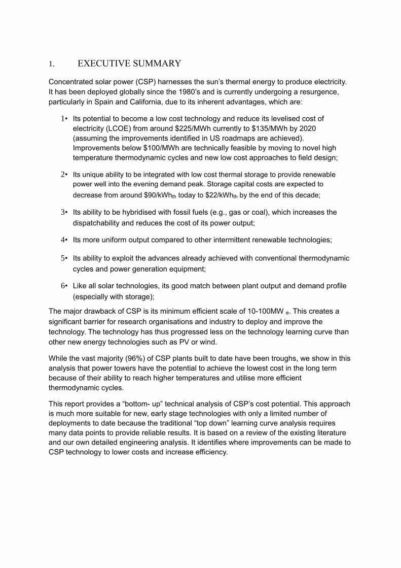
1. EXECUTIVE SUMMARY

Concentrated solar power (CSP) harnesses the sun’s thermal energy to produce electricity.It has been deployed globally since the 1980’s and is currently undergoing a resurgence, particularly in Spain and California, due to its inherent advantages, which are:

1• Its potential to become a low cost technology and reduce its levelised cost of electricity (LCOE) from around $225/MWh currently to $135/MWh by 2020 (assuming the improvements identified in US roadmaps are achieved). Improvements below $100/MWh are technically feasible by moving to novel high temperature thermodynamic cycles and new low cost approaches to field design;

2• Its unique ability to be integrated with low cost thermal storage to provide renewable power well into the evening demand peak. Storage capital costs are expected to

decrease from around $90/kWhth today to $22/kWhth by the end of this decade;

3• Its ability to be hybridised with fossil fuels (e.g., gas or coal), which increases the

dispatchability and reduces the cost of its power output;

4• Its more uniform output compared to other intermittent renewable technologies;

5• Its ability to exploit the advances already achieved with conventional thermodynamic

cycles and power generation equipment;

6• Like all solar technologies, its good match between plant output and demand profile

(especially with storage);

The major drawback of CSP is its minimum efficient scale of 10-100MW e. This creates a

significant barrier for research organisations and industry to deploy and improve the technology. The technology has thus progressed less on the technology learning curve thanother new energy technologies such as PV or wind.

While the vast majority (96%) of CSP plants built to date have been troughs, we show in thisanalysis that power towers have the potential to achieve the lowest cost in the long term because of their ability to reach higher temperatures and utilise more efficient thermodynamic cycles.

This report provides a “bottom- up” technical analysis of CSP’s cost potential. This approachis much more suitable for new, early stage technologies with only a limited number of deployments to date because the traditional “top down” learning curve analysis requires many data points to provide reliable results. It is based on a review of the existing literature and our own detailed engineering analysis. It identifies where improvements can be made toCSP technology to lower costs and increase efficiency.

2. INTRODUCTION

The objective of this document is to analyse the key cost drivers of CSP and identify the technological development needed to achieve competitive electricity production costs. It is recognised that this is a capital intensive technology and improvements in electricity production costs are most likely to result from a combination of “learning through doing” to drive down capital costs and also through technological innovation and improved conversionefficiencies. Finance and risk is also a factor with these technologies due to the significant investment required for a typical CSP plant compared to other technologies such as PV

which can be installed at the kWe scale with comparatively modest project costs.

The report was prepared as input to the Garnaut Review Update in a relatively short time

frame, and therefore is not intended to be comprehensive.

3. CSP TECHNOLOGIES

Nearly all of the world’s electricity, whether coal, gas or nuclear, is generated by first heatinga fluid. Concentrating solar thermal power is simply another means of generating a hot fluid that can then be used downstream in conventional power generation equipment such as steam turbines. Steam turbines become more efficient with higher temperatures.

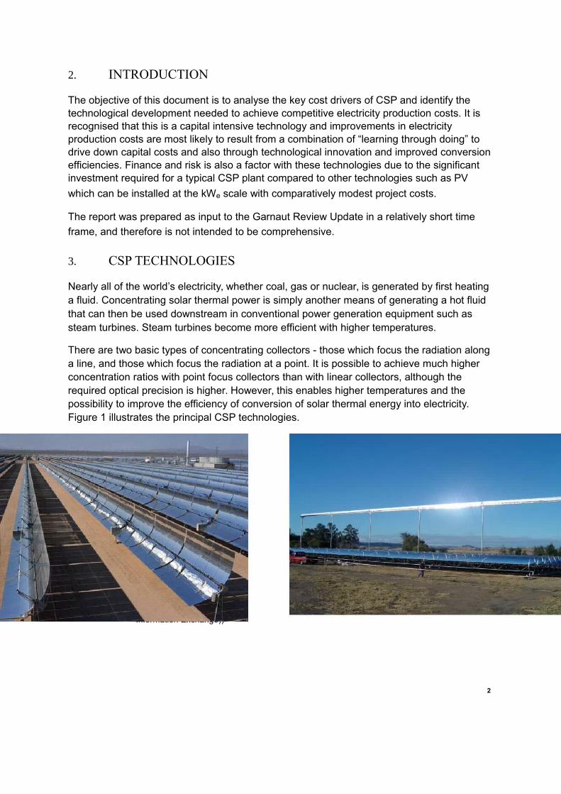
There are two basic types of concentrating collectors - those which focus the radiation alonga line, and those which focus the radiation at a point. It is possible to achieve much higher concentration ratios with point focus collectors than with linear collectors, although the required optical precision is higher. However, this enables higher temperatures and the possibility to improve the efficiency of conversion of solar thermal energy into electricity. Figure 1 illustrates the principal CSP technologies.

Parabolic troughs at Kramer Junction, CaliforniaLinear Fresnel pilot plant at Liddell Power Station,

NSW Australia. (Credit: Solar Heat and Power)(Credit: Warren Gretz (DOE/NREL PhotographicInformation Exchange))

2

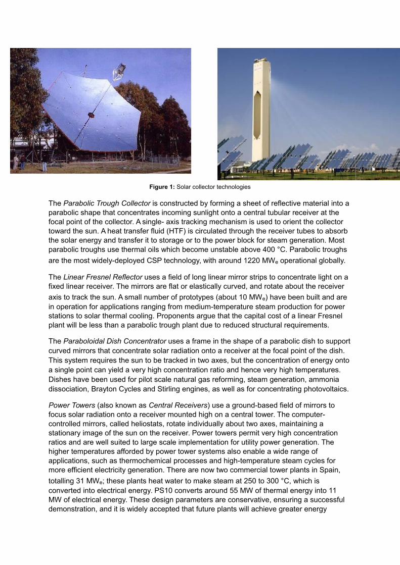
The big solar dish at the Australian National University,

Canberra (Credit: ANU) PS10 Power Tower ( Planta Solar 10) – near Seville in Spain (Credit: Solucar)

Figure 1: Solar collector technologies

The Parabolic Trough Collector is constructed by forming a sheet of reflective material into aparabolic shape that concentrates incoming sunlight onto a central tubular receiver at the focal point of the collector. A single- axis tracking mechanism is used to orient the collector toward the sun. A heat transfer fluid (HTF) is circulated through the receiver tubes to absorb the solar energy and transfer it to storage or to the power block for steam generation. Most parabolic troughs use thermal oils which become unstable above 400 °C. Parabolic troughs

are the most widely-deployed CSP technology, with around 1220 MWe operational globally.

The Linear Fresnel Reflector uses a field of long linear mirror strips to concentrate light on afixed linear receiver. The mirrors are flat or elastically curved, and rotate about the receiver

axis to track the sun. A small number of prototypes (about 10 MWe) have been built and arein operation for applications ranging from medium-temperature steam production for power stations to solar thermal cooling. Proponents argue that the capital cost of a linear Fresnel plant will be less than a parabolic trough plant due to reduced structural requirements.

The Paraboloidal Dish Concentrator uses a frame in the shape of a parabolic dish to supportcurved mirrors that concentrate solar radiation onto a receiver at the focal point of the dish. This system requires the sun to be tracked in two axes, but the concentration of energy ontoa single point can yield a very high concentration ratio and hence very high temperatures. Dishes have been used for pilot scale natural gas reforming, steam generation, ammonia dissociation, Brayton Cycles and Stirling engines, as well as for concentrating photovoltaics.

Power Towers (also known as Central Receivers) use a ground-based field of mirrors to focus solar radiation onto a receiver mounted high on a central tower. The computer-controlled mirrors, called heliostats, rotate individually about two axes, maintaining a stationary image of the sun on the receiver. Power towers permit very high concentration ratios and are well suited to large scale implementation for utility power generation. The higher temperatures afforded by power tower systems also enable a wide range of applications, such as thermochemical processes and high-temperature steam cycles for more efficient electricity generation. There are now two commercial tower plants in Spain,

totalling 31 MWe; these plants heat water to make steam at 250 to 300 °C, which is converted into electrical energy. PS10 converts around 55 MW of thermal energy into 11 MW of electrical energy. These design parameters are conservative, ensuring a successfuldemonstration, and it is widely accepted that future plants will achieve greater energy

conversion efficiencies utilising higher steam temperatures. A third plant to be commissioned

in early 2011 will use molten salt to increase steam temperatures to around 550 ºC.

The power cycle of conventional CSP plants is similar to those employed in coal fired power stations, based on a Rankine steam cycle. However, steam turbines used in solar plants are

typically smaller than those used in current state of the art fossil plants (commonly 50 MWe

compared to 600 MWe, due primarily to regulatory limits associated with feed-in tariffs). Mostdeployment to date has also used lower steam temperatures, up to 380 °C compared to up to 600 °C in fossil power stations due to issues with HTF stability.

Steam cycles work by expanding the high pressure steam through a turbine which converts the energy in the steam to mechanical work which drives a generator. The efficiency of theseturbines is influenced by the pressure drop across the unit, which is a function of the “cold sink” temperature i.e., the temperature at which thermal energy is rejected from the system through cooling. Wet (evaporative) cooling provides the lowest temperature for the cold sink but results in a significant usage of water. Dry cooling is less efficient (by about 10%) but largely eliminates the consumption of water in the power cycle. However, this also results in increased capital cost for a given capacity and a higher electricity cost. In the Australian context, dry cooling may prove to be necessary in many locations due to the limited availability of water in areas with good solar resources.

Storage is another important consideration for a CSP plant. The current trend is for plants with upwards of 6 hours of storage (i.e., the amount of thermal energy required to operate the power block at full capacity for 6 hours). This allows plants to be less impacted by variations in solar radiation through the day, and to continue operating after the sun has set. Though there are increased capital costs associated with this ability due to the need for extrasolar collectors, a larger receiver system, and of course the storage system and medium itself, these costs are offset by the extra operating hours, particularly at periods of higher tariff. Current practice is to use “solar salt”, a mixture of sodium and potassium nitrate which melts at around 220 °C and is stable to about 590 °C, although there is considerable research into new materials to extend the upper temperature limit.

4. CURRENT MARKET PENETRATION

While CSP technologies have been successfully producing electricity at utility scale since the mid1980s, these early installations were followed by a significant hiatus in construction, with no new plants commissioned until 2006. Recent years have seen a significant acceleration in activity, as a result of favourable investment environments created by feed in tariffs and tax incentives in Spain and the US. Table 1 summarises current CSP plant deployment.

Table 1: Current and predicted global deployment of CSP plants (sources:

NREL Concentrating Solar Power Projects http://www.nrel.gov/csp/solarpaces/by_project.cfm and

Wikipedia http://en.wikipedia.org/wiki/List_of_solar_thermal_power_stations )

Status # Projects Capacity (GW)Operational (end 2010) 39 1.27Under construction 29 1.93In development 67 17.53

We expect that the deployment of CSP plants will continue to accelerate thus helping drive

capital costs down through “learning by doing” effects (see Section 7).

4

5. LEVELISED COST OF ELECTRICITY (LCOE)

The LCOE is a useful measure of the cost competitiveness of a generation technology, although when comparing values it is important to be aware of the assumptions that are embedded. For a solar plant, these may include site specific factors such as the (Direct Normal Irradiance) DNI and meteorology of a particular location, as well as more general assumptions about the life of the plant and construction period, interest rate, and capital andoperating costs. In addition, the calculation methodology used to determine the LCOE can vary. Other costs can also be included or excluded, such as interest during construction, decommissioning costs, different levels of contingency, insurance, tax, adjustment factors, and financial incentives such as feed-in-tariffs etc.

Storage has a significant impact as it increases the capital cost but allows the plant to operate for longer. The optimum amount of storage depends on the relative cost of extra collectors, tanks and storage medium, but is also dependent on the revenue generated bythe plant. Electricity prices are higher during the day when demand is greater and remain high into the early evening. Thus storage offers the possibility to earn higher revenue. Optimising the overall design thus becomes more complex than simply minimising LCOE,and is dependent on the market into which the electricity is sold.

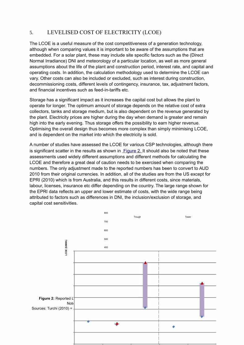
A number of studies have assessed the LCOE for various CSP technologies, although thereis significant scatter in the results as shown in Figure 2. It should also be noted that these assessments used widely different assumptions and different methods for calculating the LCOE and therefore a great deal of caution needs to be exercised when comparing the numbers. The only adjustment made to the reported numbers has been to convert to AUD 2010 from their original currencies. In addition, all of the studies are from the US except for EPRI (2010) which is from Australia, and this results in different costs, since materials, labour, licenses, insurance etc differ depending on the country. The large range shown for the EPRI data reflects an upper and lower estimate of costs, with the wide range being attributed to factors such as differences in DNI, the inclusion/exclusion of storage, and capital cost sensitivities.

800

Trough Tower

700

600

($/M

Wh

) 500

400

LC

OE

300

200

100

0

Turchi (2010) NREL (2010) EPRI (2010) Turchi (2010) EPRI (2010)

Figure 2: Reported LCOE from various studies for projected trough and tower plants in the year 2010.Note that EPRI (2010) is for a plant commissioned in the year 2015.

Sources: Turchi (2010) = (Turchi et al., 2010); S&L (2003) = (Sargent and Lundy LLC Consulting Group, 2003);

NREL (2010) = (Turchi, 2010) and EPRI (2010) = (EPRI Palo Alto CA and Commonwealth of Australia, 2010)

There are a number of prominent earlier studies which also determined the cost and potential of CSP, notably a report by Sargent and Lundy (Sargent and Lundy LLC ConsultingGroup, 2003) and the European Concentrated Solar Therm al Road-Mapping study ECOSTAR (Pitz- Paal et al., 2005) . However, it is difficult to compare projections from thesestudies because key assumptions about the deployment of CSP were not realised which affects learning curve cost reductions.

Our analysis has assumed a 20 year plant life and a weighted average cost of capital of 7%.

6. CAPITAL COST EVALUATION

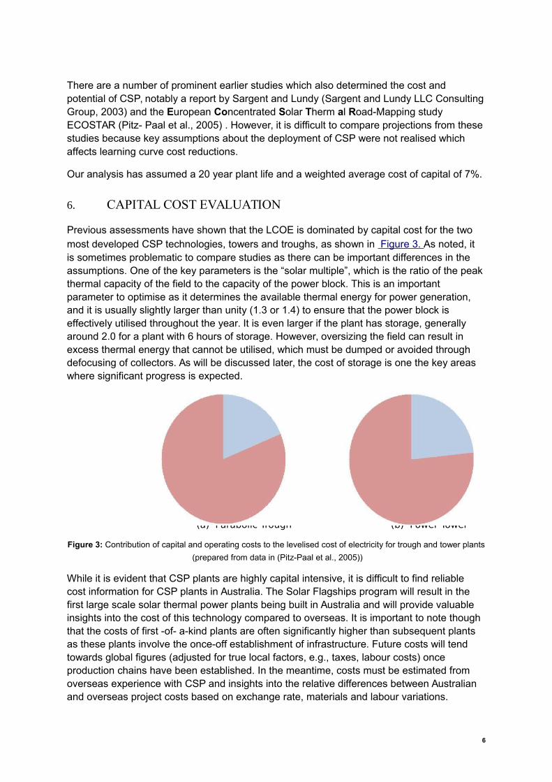
Previous assessments have shown that the LCOE is dominated by capital cost for the two most developed CSP technologies, towers and troughs, as shown in Figure 3. As noted, it is sometimes problematic to compare studies as there can be important differences in the assumptions. One of the key parameters is the “solar multiple”, which is the ratio of the peakthermal capacity of the field to the capacity of the power block. This is an important parameter to optimise as it determines the available thermal energy for power generation, and it is usually slightly larger than unity (1.3 or 1.4) to ensure that the power block is effectively utilised throughout the year. It is even larger if the plant has storage, generally around 2.0 for a plant with 6 hours of storage. However, oversizing the field can result in excess thermal energy that cannot be utilised, which must be dumped or avoided through defocusing of collectors. As will be discussed later, the cost of storage is one the key areas where significant progress is expected.

annual annualO&M costs O&M

costs19% 23%

annual annualfinancing & financing &insurance insurance

costs costs81% 77%

(a) Parabolic Trough (b) Power Tower

Figure 3: Contribution of capital and operating costs to the levelised cost of electricity for trough and tower plants

(prepared from data in (Pitz-Paal et al., 2005))

While it is evident that CSP plants are highly capital intensive, it is difficult to find reliable cost information for CSP plants in Australia. The Solar Flagships program will result in the first large scale solar thermal power plants being built in Australia and will provide valuable insights into the cost of this technology compared to overseas. It is important to note though that the costs of first -of- a-kind plants are often significantly higher than subsequent plants as these plants involve the once-off establishment of infrastructure. Future costs will tend towards global figures (adjusted for true local factors, e.g., taxes, labour costs) once production chains have been established. In the meantime, costs must be estimated from overseas experience with CSP and insights into the relative differences between Australian and overseas project costs based on exchange rate, materials and labour variations.

6

6.1 Capital cos t es timates from previous s tudies

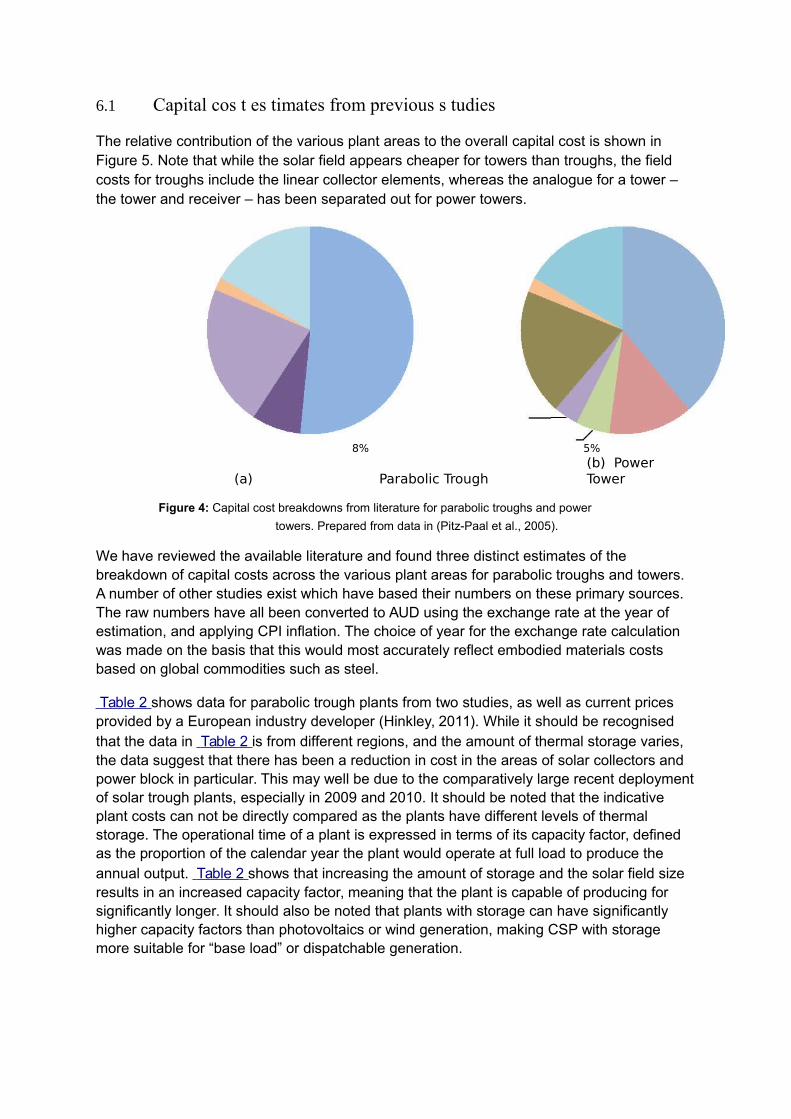
The relative contribution of the various plant areas to the overall capital cost is shown in Figure 5. Note that while the solar field appears cheaper for towers than troughs, the field costs for troughs include the linear collector elements, whereas the analogue for a tower –the tower and receiver – has been separated out for power towers.

indirect indirect

land costs land costssolar

2% 17% 2% 17%field39%

power solar powerblockblock field20%

22% 51%receiver

storage 13%

storage 4% tower8% 5%

(a) Parabolic Trough(b) Power Tower

Figure 4: Capital cost breakdowns from literature for parabolic troughs and power

towers. Prepared from data in (Pitz-Paal et al., 2005).

We have reviewed the available literature and found three distinct estimates of the breakdown of capital costs across the various plant areas for parabolic troughs and towers.A number of other studies exist which have based their numbers on these primary sources.The raw numbers have all been converted to AUD using the exchange rate at the year of estimation, and applying CPI inflation. The choice of year for the exchange rate calculation was made on the basis that this would most accurately reflect embodied materials costs based on global commodities such as steel.

Table 2 shows data for parabolic trough plants from two studies, as well as current prices provided by a European industry developer (Hinkley, 2011). While it should be recognised that the data in Table 2 is from different regions, and the amount of thermal storage varies, the data suggest that there has been a reduction in cost in the areas of solar collectors and power block in particular. This may well be due to the comparatively large recent deploymentof solar trough plants, especially in 2009 and 2010. It should be noted that the indicative plant costs can not be directly compared as the plants have different levels of thermal storage. The operational time of a plant is expressed in terms of its capacity factor, defined as the proportion of the calendar year the plant would operate at full load to produce the annual output. Table 2 shows that increasing the amount of storage and the solar field size results in an increased capacity factor, meaning that the plant is capable of producing for significantly longer. It should also be noted that plants with storage can have significantly higher capacity factors than photovoltaics or wind generation, making CSP with storage more suitable for “base load” or dispatchable generation.

Table 2: Comparison of estimated capital costs of the key areas from various studies on parabolic trough plants

(Prepared from data from Ecostar (2005) = (Pitz-Paal et al., 2005) ,Turchi (2010) = (Turchi et al., 2010) and

Developer (2011) = (Hinkley, 2011)).

Ecostar (2005) Turchi (2010) Developer (2011)Net Plant Size (MWe) 50 100 50Solar Multiple 1.4 2.0 1.3 (est.)Capacity Factor (%) 28.5 40.0 23.0Site Improvements ($/m2 field) 4 27 14Solar Field ($/m2 field) 385 320 538HTF System ($/m2 field) 98 39Storage ($/kWhth) 58 87 (79)Power Block, BOP ($/kWe gross) 1327 1021 2885Indicative Plant Cost ($/kWe net) 6600 8688 7501

(3 hours storage, (6 hours storage, (no storage,wet cooling) wet cooling) wet cooling)

Table 3 summarises two estimates for towers with molten salt from a European and a US source. The data suggest that there has been some moderate cost reduction in the heliostatfield and tower/receiver costs, although the power block costs are comparable and storage costs are higher for the more recent study. It is also interesting to note that the power block and balance of plant costs are estimated as being higher for tower plants than trough plants,despite using essentially the same technology. Storage is considerably cheaper for molten salt towers than troughs using thermal oil as the HTF because the difference between the hot and cold tanks is much greater (~280 degrees for towers compared to ~100 degrees for troughs). Note that the current commercial tower PS10 has around 0.4 hours of steam

storage at an estimated $187/kWhth.

Table 3: Comparison of estimated capital costs of the key areas from various studies on power tower plants.

(Prepared from data from Ecostar (2005) = (Pitz-Paal et al., 2005) and Sandia (2010) = (Gary et al., 2010))

Ecostar (2005) Sandia (2010)Net plant size (MWe) 51 100Solar multiple (unitless) 1.4 2.1Capacity factor (%) 33 48Storage ($/kWhth) 24 33Tower & Receiver ($/kWth) 216 217Solar Field ($/m2) 266 217Power block ($/kWe) 1298 1380Indicative plant cost ($/kWe) 6494 8066

(3 hrs storage, (9 hours storage,wet cooling) wet cooling)

6.2 Capital cos t es timates bas ed on “bottom -up” evaluation

Aurecon Australia have used their considerable experience in the engineering, design and project management of pulverised coal and gas fired thermal power plants to build up estimated plant costs for a power tower plant. Aurecon’s cost estimate was based on a plant design

specification developed by CSIRO for a 100 MWe plant located in central Queensland (Longreach) using NREL’s Solar Advisor Model (SAM) . SAM is a comprehensive model developed to perform techno-economic evaluations of various solar technologies, and can develop plant designs and LCOE based on climate data for a specified location. SAM models an entire CSP plant from the collector field through to the power block, and allows

8

the user to specify key parameters such as the per unit capital cost of different plant areas

(e.g., $/kW e), the amount of thermal storage and whether the plant uses wet or dry cooling. Longreach was selected as it has a good solar resource and reasonable infrastructure connections, as well as good meteorological information for SAM.

Full details of the plant design and methodology for determining the cost estimates can be

found in Appendix A. Two designs were considered, a 100 MWe plant with and without 6

hours of thermal storage. Note that these costs are based on the “nth plant” rather than the expected cost for the construction of the first plant in Australia. These figures therefore represent what we believe is the potential capital cost of CSP in Australia based on current materials and labour prices and include up to date estimates of the power block costs. The greatest uncertainties are in the solar components, as these will require the establishment ofmanufacturing and supply chains which would add significantly to the cost of the first plants constructed in Australia. However, the estimates confirm that there is no reason why CSP plants cannot be constructed in Australia at prices in line or below overseas in the longer term.

Table 4: Estimated capital cost for a 100 MW power tower constructed in Australia

Estimated cost (A$ million)Equipment area Unit Cost No storage With storageSite preparation & civils $30 /kWe,net 30.0 30.0Solar Field $142 /m2 101.8 143.2Tower $29 /kWth 11.5 14.5Receiver $19 /kWth 9.2 9.7Molten Salt and Storage Systems $12 /kWhth 12.6 20.8Turbine systems (inc generator) $424 /kWe,gross 46.0 46.6Steam generation $187 /kWe,gross 20.6 20.6Air Cooled Condenser (ACC) $371 /kWe,gross 40.8 40.8Electrical $180 /kWe,net 18.0 18.0Controls $100 /kWe,net 10.0 10.0Fire Services $40 /kWe,net 4.0 4.0Spares (allow 5%) 15.2 17.9Owner & contractor costs (30%) 95.9 112.9Total Capital Cost 415.8 489.0Indicative Plant Cost (dry cooled) $/kWe 4158 4890

7. COST TRAJ ECTORIES – CSP PRICES REDUCE WITHDEPLOYMENT

Deployment is one of the most important factors in the reduction of cost for new technologies such as CSP. This is typically expressed in terms of experience curves, as shown in Figure 5. The calculated learning rate over all CSP installations to date is a 15% reduction per doubling of cumulative deployment. It reflects cost savings from both economies of scale in manufacturing and technical innovation. Given the small number installations and the stop start deployment of CSP plants, the error bar on this figure is expected to be significant. More established renewables have demonstrated comparable learning rates, e.g., 20% for photovoltaics and 15% for wind (Hayward et al., 2011).

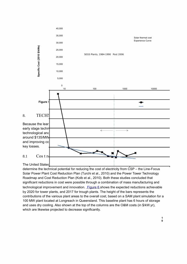
40,000

35,000Solar thermal cost

30,000Experience Curve

$/k

We)

25,000

SEGS Plants, 1984-1990 Post 2006

(20

10 20,000

Co

st

15,000

Sp

ecif

ic

10,000

5,000

0

10 100 1000 10000

Cumulative Capacity (MW)

Figure 5: CSP historical cost data vs. cumulative capacity with a fitted experience curve

(Prepared from data from (Hayward et al., 2011))

8. TECHNOLOGY POTENTIAL

Because the learning rate methodology discussed in the previous section has limitations forearly stage technologies, we will now analyse the potential for LCOE reduction based on a technological analysis. We find the LCOE can be reduced from the current $225/MWh to around $135/MWh by 2020 through a combination of reduced capital cost through learning,and improving conversion efficiency by moving to higher temperature cycles and eliminatingkey losses.

8.1 Cos t reduction s tudies

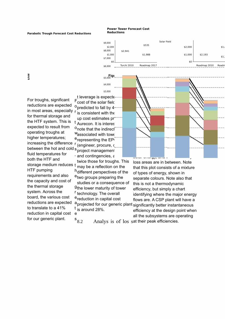
The United States Department of Energy (DOE) has commissioned two recent studies to determine the technical potential for reducing the cost of electricity from CSP – the Line-Focus Solar Power Plant Cost Reduction Plan (Turchi et al., 2010) and the Power Tower Technology Roadmap and Cost Reduction Plan (Kolb et al., 2010). Both these studies concluded that significant reductions in cost were possible through a combination of mass manufacturing and

technological improvement and innovation. Figure 6 shows the expected reductions achievable by 2020 for tower plants, and 2017 for trough plants. The height of the bars represents the contributions of the various plant areas to the overall cost, based on a SAM plant simulation for a100 MW plant located at Longreach in Queensland. This baseline plant has 6 hours of storage and uses dry cooling. Also shown at the top of the columns are the O&M costs (in $/kW.yr), which are likewise projected to decrease significantly.

10

Parabolic Trough Forecast Cost Reductions

Power Tower Forecast Cost Reductions

$/k

W

$9,000

$8,000

$7,000

$6,000

$5,000

$4,000

$3,000

Solar Field

$2,000$535

$2,000 $1,471

$2,941

$2,193$1,000 $1,988 $1,000$1,316

$0 $0

Roadmap 2010 Roadmap 2020Turchi 2010 Roadmap 2017

Figure 6: Projected parabolic trough and power tower

cost reductions over the current decade

(Data from (Kolb et al., 2010, Kutscher et

al., 2010, Turchi et al., 2010))

For troughs, significant reductions are expected in most areas, especially for thermal storage and the HTF system. This is expected to result from operating troughs at higher temperatures; increasing the difference between the hot and coldfluid temperatures for both the HTF and storage medium reduces HTF pumping requirements and also the capacity and cost of the thermal storage system. Across the board, the various cost reductions are expected to translate to a 41% reduction in capital cost for our generic plant.

For towers, the greates

t leverage is expected in the cost of the solar field, which ispredicted to fall by 40%. This is consistent with the ground up cost estimates provided byAurecon. It is interesting to note that the indirect costs associated with towers, representing the EPC (engineer, procure, construct) project management costs and contingencies, are almosttwice those for troughs. This may be a reflection on the different perspectives of the two groups preparing the studies or a consequence of the lower maturity of tower technology. The overall reduction in capital cost projected for our generic plantis around 28%.

8.2 Analys is of los s

es and opportunities

SAM models the energy flows in a CSP plant by determining the losses in each subsystem of the overall plant. Figure 7 shows annual average data from SAM fora tower plant with 6 hours storage.The plot shows how the net electrical output of the plant is related to the potential incident solar energy, and where the key loss areas are in between. Note that this plot consists of a mixture of types of energy, shown in separate colours. Note also that this is not a thermodynamic efficiency, but simply a chart identifying where the major energyflows are. A CSP plant will have a significantly better instantaneous efficiency at the design point whenall the subsystems are operating at their peak efficiencies.

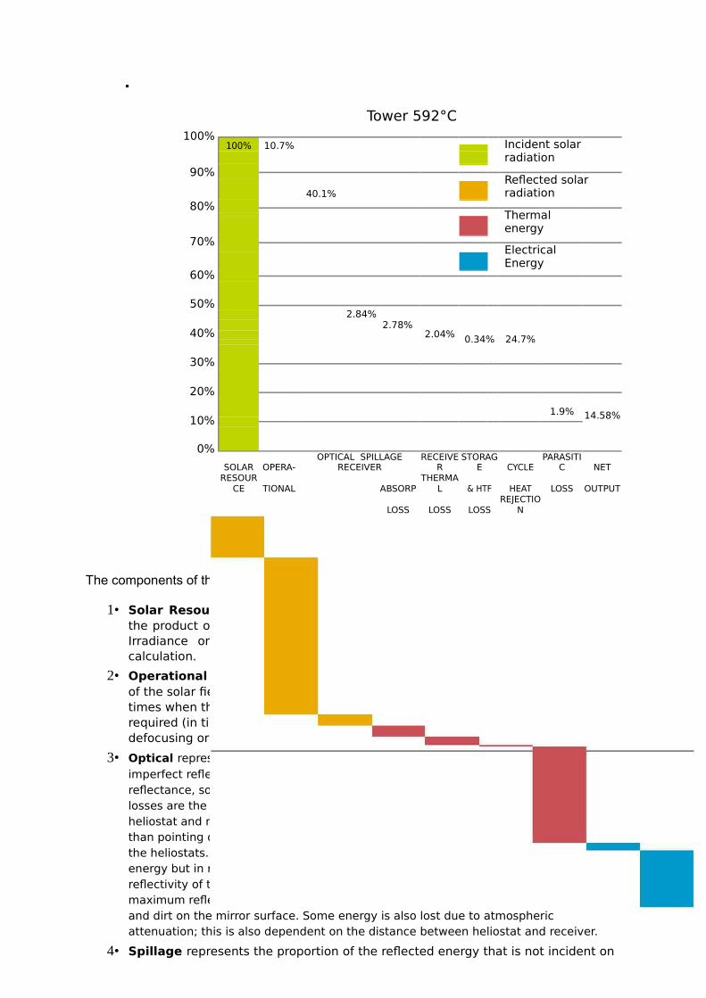
Tower 592°C100%

100% 10.7% Incident solar radiation

90%

40.1%Reflected solar radiation

80%Thermal energy

70%Electrical Energy

60%

50%2.84%

40%2.78%

2.04% 0.34% 24.7%

30%

20%

1.9% 14.58%10%

0%

SOLAR OPERA-OPTICAL SPILLAGE

RECEIVERRECEIVE

RSTORAG

E CYCLEPARASITI

C NETRESOUR

CE TIONAL ABSORPTHERMA

L & HTF HEAT LOSS OUTPUT

LOSS LOSS LOSSREJECTIO

N

Figure 7: Energy flow diagram for a power tower CSP plant

The components of the energy diagram are as follows:

1• Solar Resource represents the theoretical amount of energy available, and isthe product of the solar radiation on a surface normal to the sun (Direct NormalIrradiance or DNI) and the total mirror area. This is an annual averagecalculation.

2• Operational represents the energy that is not collected due to non-utilisation of the solar field from mechanical unavailability of the overall plant, as well as times when the power cycle is fully loaded and additional thermal energy is not required (in times of peak DNI), and energy is not collected or utilized through defocusing or dumping.

3• Optical represents the amount of energy that is lost due to geometric factors and imperfect reflection of the available energy. It includes effects from cosine losses, reflectance, soiling, shading and blocking and from atmospheric attenuation. Cosine losses are the geometric losses that result from the relative position of the sun, heliostat and receiver (because the heliostat directs energy onto the receiver rather than pointing directly at the sun). There are also losses due to shading and blocking ofthe heliostats. These losses together total about 20% of the theoretically possible energy but in reality cannot be eliminated. Reflectance refers to the losses due to the reflectivity of the mirror surface – even high performance low iron glass mirrors have amaximum reflectivity of about 96%. Soiling refers to losses in reflectivity due to dust and dirt on the mirror surface. Some energy is also lost due to atmospheric attenuation; this is also dependent on the distance between heliostat and receiver.

4• Spillage represents the proportion of the reflected energy that is not incident on

the receiver surface due to mirror quality or errors in positioning.

5• Receiver absorption losses refer to the amount of energy that is reflected by the receiver surfaces. Even high absorption coatings typically have a maximum absorbance of 94% i.e., 94% of the incident concentrated solar radiation is converted to thermal energy.

12

1• Receiver Thermal Losses represent the thermal losses from the receiverdue to convection and radiation losses.

2• Storage & HTF Loss represents the amount of thermal energy that is lostfrom piping and thermal storage systems. These losses are normally very lowdue to insulation.

3• Cycle heat rejection refers to the thermal energy that the power cycle is not able to convert to electricity, which is rejected as waste heat in the cooling system. This is discussed in more detail below.

4• Parasitic Loss refers to the energy consumed by the plant itself to produce electricity, and consists primarily of the electrical requirement for HTF pumping along with energy used for control of the positioning of the heliostats (minor). Theparasitic loss is typically around 5-10% of the gross electrical output of the plant depending on the level of storage. It may be possible to reduce these losses as in conventional fossil plants through the use of steam driven rather than electric pumps.

5• Net Output is the electricity produced by the plant, after all internal losses havebeen accounted for.

Figure 7 suggests that the priority areas for improvement are the reduction of optical losses and the cycle heat rejection. The bulk of the optical “losses” are in fact a function of geometry and themovement of the sun through the day, which can not be eliminated. It is certainly possible to optimise the field layout to minimise the amount of shading and blocking with existing design tools. Likewise, it is widely recognised that the reflectance is a key parameter, and there is little room for improvement on the performance of current materials, although there is some interest indeveloping surface coatings to prevent dust adhesion and minimise water consumption for cleaning. The major areas of work relating to the optics of towers are around improving the precision of the heliostats, and reducing their capital cost.

The other major area of energy loss is in the power cycle, and there are a number of options

for improving performance in this area.

8.2.1 Improving the efficiency of power convers ion

The maximum steam temperature in the power cycle is the primary driver of the theoretical power that can be extracted from the thermal energy in a CSP plant. The maximum amountof work that can be done using a heat engine is expressed by the Carnot effic iency:

= 1 −

ηℎ

Where ηis the efficiency, Tc the absolute temperature of the cold sink and Th the absolute temperature of the hot fluid. This equation defines the thermodynamic upper limit for the efficiency of a heat engine; a real cycle based on steam has other losses and inefficiencies and will reach about two thirds of the Carnot cycle efficiency. The real cycle used in steam power plants is the Rankine cycle (see Appendix B) . The efficiency of the Rankine cycle depends on the average temperature at which heat is supplied and the average temperatureat which heat is rejected. Any changes that increase the temperature that is supplied or decrease the average temperature that is rejected will increase the Rankine cycle efficiency.

As noted earlier, CSP plants have typically utilised much lower steam temperatures and pressure than current industry practice for pulverised coal plants. Parabolic trough plants have

been limited by the decomposition temperature of the thermal oil used as the heat transfer fluid

to temperatures less than 390 °C, although a 5 MW e demonstration plant has recently been constructed in Sicily using molten salt as the HTF, reaching an outlet temperature of 550 °C from the solar field (NREL, 2011), Similarly, the two operating power

tower plants (PS10 and PS20) have used rather conservative steam conditions of 250-300 °C (ibid), as they are the first of their type. However, a third plant being commissioned in 2011, Gemasolar, will use molten salt in the receiver to attain an outlet temperature of 565 °C (ibid). It is generally accepted that increasing the temperature at which steam can be generated will result in significant improvements in efficiency and reduction in the LCOE. Wewill now explore this premise based on data from SAM modelling, our harmonised cost data presented previously, and data for commercially available steam turbines.

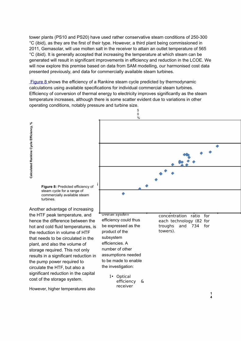
Figure 8 shows the efficiency of a Rankine steam cycle predicted by thermodynamic calculations using available specifications for individual commercial steam turbines. Efficiency of conversion of thermal energy to electricity improves significantly as the steamtemperature increases, although there is some scatter evident due to variations in other operating conditions, notably pressure and turbine size.

Ca

lcu

late

d R

an

kin

e C

ycle

Eff

icie

nc

y, %

50%

Rankine cycleefficiency

45%

40%

35%

30%

350 400 450 500 550

600 650

Temp (DegC)

Figure 8: Predicted efficiency of steam cycle for a range of commercially available steam turbines.

Another advantage of increasing the HTF peak temperature, and hence the difference between the hot and cold fluid temperatures, isthe reduction in volume of HTF that needs to be circulated in the plant, and also the volume of storage required. This not only results in a significant reduction inthe pump power required to circulate the HTF, but also a significant reduction in the capital cost of the storage system.

However, higher temperatures also

i investigate how the efficiency of the plant

areas identified in Figure 7 varied with temperature. The overall system efficiency could thus be expressed as the product of the subsystem efficiencies. A number of other assumptions needed to be made to enablethe investigation:

1• Opticalefficiency &receiver

absorption: assumed tobe constant;

2• Receiver re-radiationlosses: modelled usingthe Stefan-Boltzmannlaw using constantconcentration ratio foreach technology (82 fortroughs and 734 fortowers).

14

1• Convective losses assumed to increase linearly with temperature, based on a temperature difference of 80° between tower receiver surface and HTF. For troughs, difference of 330° between collector tube and outside of glass (i.e., 60° C at design point)

2• HTF has a minimum working temperature of 290 °C

3• Power block efficiency: modelled using data from Figure 8

4• Parasitic losses: assumed proportional to HTF temperature difference andamount of HTF to be circulated

5• Project risk was assumed to be the same (18.5% contingency) for towers andtrough plants

6• Power block costs were assumed to be the same ($1021 /kWe) for towers andtrough plants

The plant was resized based on the overall efficiency by adjusting the size of the solar field,tower, receiver and power block to give the same net output of electricity. Note that the minimum working temperature of the HTF causes an asymptotic increase in the LCOE at lower temperatures due to lower overall efficiencies, which increases capital costs due to increases in the collector area required. This is a consequence of both increases in HTF pumping requirements and decreased efficiency in the power cycle.

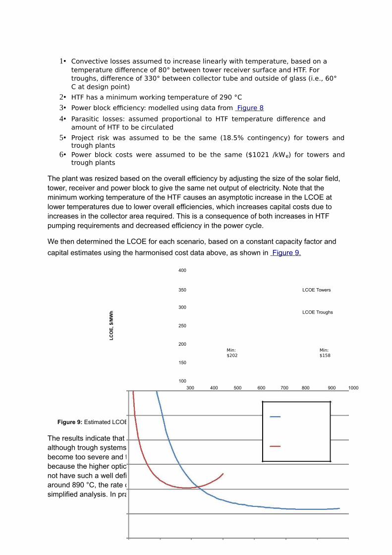
We then determined the LCOE for each scenario, based on a constant capacity factor and

capital estimates using the harmonised cost data above, as shown in Figure 9.

400

350 LCOE Towers

$/M

Wh

300LCOE Troughs

250

LC

OE

,

200Min: Min:$202 $158

150

100

300 400 500 600 700 800 900 1000

Upper Temperature of HTF, C

Figure 9: Estimated LCOE for “current generation” troughs and tower for varying HTF peak temperatures.

The results indicate that LCOE generally decreases as the HTF temperature increases, although trough systems have a minimum around 490 °C beyond which thermal losses become too severe and the LCOE increases again. This is less of an issue for towers, because the higher optical concentration results in a smaller area for re-radiation. Towers do not have such a well defined minimum LCOE; while the LCOE continues decrease up to around 890 °C, the rate of reduction slows with increasing temperature. Note that this is a simplified analysis. In practice, a number of other factors must be considered including the

stability of the HTF itself (beyond 600 °C), the ability of the receiver materials to withstand high temperatures especially in hot spots, and finding an appropriate power conversion cycle. If these requirements can be met, further decreases in LCOE of 10 % may be possible at a temperature of 750°C for example.

9. CONCLUSIONS:

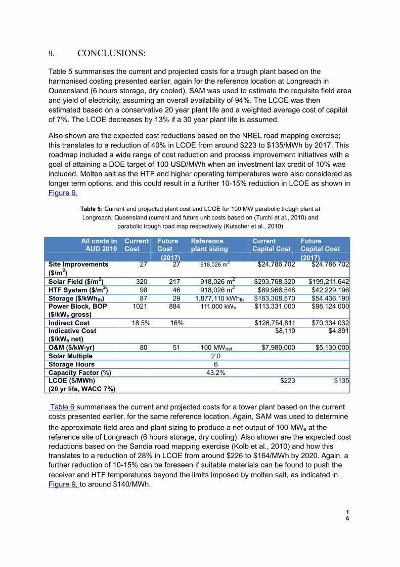
Table 5 summarises the current and projected costs for a trough plant based on the harmonised costing presented earlier, again for the reference location at Longreach in Queensland (6 hours storage, dry cooled). SAM was used to estimate the requisite field areaand yield of electricity, assuming an overall availability of 94%. The LCOE was then estimated based on a conservative 20 year plant life and a weighted average cost of capital of 7%. The LCOE decreases by 13% if a 30 year plant life is assumed.

Also shown are the expected cost reductions based on the NREL road mapping exercise; this translates to a reduction of 40% in LCOE from around $223 to $135/MWh by 2017. This roadmap included a wide range of cost reduction and process improvement initiatives with a goal of attaining a DOE target of 100 USD/MWh when an investment tax credit of 10% was included. Molten salt as the HTF and higher operating temperatures were also considered aslonger term options, and this could result in a further 10-15% reduction in LCOE as shown inFigure 9.

Table 5: Current and projected plant cost and LCOE for 100 MW parabolic trough plant at

Longreach, Queensland (current and future unit costs based on (Turchi et al., 2010) and

parabolic trough road map respectively (Kutscher et al., 2010)

All costs in Current Future Reference Current FutureAUD 2010 Cost Cost plant sizing Capital Cost Capital Cost

(2017) (2017)Site Improvements 27 27 918,026 m2 $24,786,702 $24,786,702($/m2)Solar Field ($/m2) 320 217 918,026 m2 $293,768,320 $199,211,642HTF System ($/m2) 98 46 918,026 m2 $89,966,548 $42,229,196Storage ($/kWhth) 87 29 1,877,110 kWhth $163,308,570 $54,436,190Power Block, BOP 1021 884 111,000 kWe $113,331,000 $98,124,000($/kWe gross)Indirect Cost 18.5% 16% $126,754,811 $70,334,032Indicative Cost $8,119 $4,891($/kWe net)O&M ($/kW-yr) 80 51 100 MWnet $7,980,000 $5,130,000Solar Multiple 2.0Storage Hours 6Capacity Factor (%) 43.2%LCOE ($/MWh) $223 $135(20 yr life, WACC 7%)

Table 6 summarises the current and projected costs for a tower plant based on the current costs presented earlier, for the same reference location. Again, SAM was used to determine

the approximate field area and plant sizing to produce a net output of 100 MWe at the reference site of Longreach (6 hours storage, dry cooling). Also shown are the expected costreductions based on the Sandia road mapping exercise (Kolb et al., 2010) and how this translates to a reduction of 28% in LCOE from around $226 to $164/MWh by 2020. Again, a further reduction of 10-15% can be foreseen if suitable materials can be found to push the receiver and HTF temperatures beyond the limits imposed by molten salt, as indicated in Figure 9, to around $140/MWh.

16

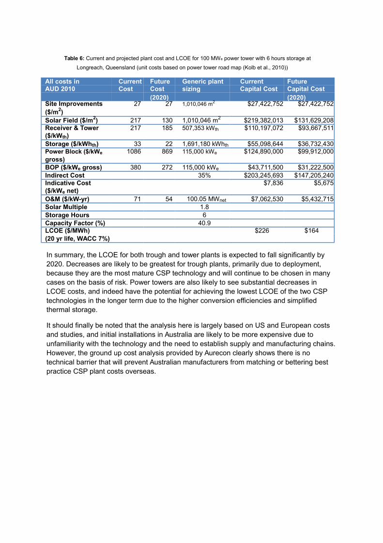
Table 6: Current and projected plant cost and LCOE for 100 MWe power tower with 6 hours storage at

Longreach, Queensland (unit costs based on power tower road map (Kolb et al., 2010))

All costs in Current Future Generic plant Current FutureAUD 2010 Cost Cost sizing Capital Cost Capital Cost

(2020) (2020)Site Improvements 27 27 1,010,046 m2 $27,422,752 $27,422,752($/m2)Solar Field ($/m2) 217 130 1,010,046 m2 $219,382,013 $131,629,208Receiver & Tower 217 185 507,353 kWth $110,197,072 $93,667,511($/kWth)Storage ($/kWhth) 33 22 1,691,180 kWhth $55,098,644 $36,732,430Power Block ($/kWe 1086 869 115,000 kWe $124,890,000 $99,912,000gross)BOP ($/kWe gross) 380 272 115,000 kWe $43,711,500 $31,222,500Indirect Cost 35% $203,245,693 $147,205,240Indicative Cost $7,836 $5,675($/kWe net)O&M ($/kW-yr) 71 54 100.05 MWnet $7,062,530 $5,432,715Solar Multiple 1.8Storage Hours 6Capacity Factor (%) 40.9LCOE ($/MWh) $226 $164(20 yr life, WACC 7%)

In summary, the LCOE for both trough and tower plants is expected to fall significantly by 2020. Decreases are likely to be greatest for trough plants, primarily due to deployment, because they are the most mature CSP technology and will continue to be chosen in manycases on the basis of risk. Power towers are also likely to see substantial decreases in LCOE costs, and indeed have the potential for achieving the lowest LCOE of the two CSP technologies in the longer term due to the higher conversion efficiencies and simplified thermal storage.

It should finally be noted that the analysis here is largely based on US and European costs and studies, and initial installations in Australia are likely to be more expensive due to unfamiliarity with the technology and the need to establish supply and manufacturing chains.However, the ground up cost analysis provided by Aurecon clearly shows there is no technical barrier that will prevent Australian manufacturers from matching or bettering best practice CSP plant costs overseas.

REFERENCES

EPRI PALO ALTO CA & COMMONWEALTH OF AUSTRALIA (2010) Australian Electricity Generation Technology Costs - Reference Case 2010. IN BOORAS,G. (Ed., Prepared for Department of Resources, Energy and Tourism.

GARY, J. A., CLIFFORD, K. H., MANCINI, T. R., KOLB, G. J., SIEGEL, N. P. & IVERSON, B. D. (2010) Development of a power tower technology roadmap forDOE. SolarPaces. Perpignan, France.

HAYWARD, J. A., GRAHAM, P. W. & CAMPBELL, P. K. (2011) Projections of the future costs of electricity generation technologies: an application of CSIRO'sGlobal and Local Learning Model (GALLM). CSIRO.

HINKLEY, J. (2011) Confidential industry personal communication.KOLB, G. J., HO, C. K., MANCINI, T. R. & GARY, J. A. (2010) Power tower technology

roadmap and cost reduction plan. Sandia National Laboratories (Draft, Version18, December 2010).

KUTSCHER, C., MEHOS, M., TURCHI, C. & GLATZMAIER, G. (2010) Line-focus solarpower plant cost reduction plan. NREL and Sandia.

NREL (2011) Concentrating solar power projects by project name. Golden, Colorado,NREL National Renewable Energy Laboratory.

PITZ-PAAL, R., DERSCH, J. & MILOW, B. (2005) ECOSTAR: European ConcentratedSolar Thermal Road-Mapping. DLR.

SARGENT AND LUNDY LLC CONSULTING GROUP (2003) Assessment of parabolictrough and power tower solar technology cost and performance forecasts. Chicago, Illinois, USA, NREL.

TURCHI, C. (2010) Parabolic trough reference plant for cost modeling with the Solar Advisor Model (SAM).

Golden, Colorado, NREL.TURCHI, C., MEHOS, M., HO, C. K. & KOLB, G. J. (2010) Current and future costs for

parabolic trough and power tower systems in the US market. SolarPACES 2010. Perpignan, France

18

APPENDIX A: CAPITAL ESTIMATES BASED ON “BOTTOM-UP” COSTING

Aurecon Australia used their considerable experience in the engineering, design and projectmanagement of pulverised coal and gas fired thermal power plants to build up plant cost estimates for CSP plants. CSIRO and Aurecon have developed a process design for a 100 MW plant located in central Queensland (Longreach) using power tower technology, and Aurecon have provided a cost estimate.

A.1 Methodology

Component costs for the 100 MW plant have been estimated using a “bottom-up”

approach. To achieve this, the plant was divided into 4 main areas:

1− Solar Field

2− Receiver & Tower

3− Storage and molten salt system

4− Power Block

Within each area, approximately 10 equipment items or systems were identified for detailedcosting. Depending on the particular equipment, one of the following methods was used toestimate its fabrication and installation cost. In most cases an alternative method was usedfor verification. The methods include:

1) Obtain budget estimates from suppliers: A number of the plant components are standard items used in a variety of different industrial and power generation processes. Prices were obtained from local suppliers for items of this type. Examplesinclude pumps, fans and piping.

2) Reference to Aurecon equipment cost database: A number of equipment items are used in other power generation technologies and are familiar to Aurecon. For these items, our equipment capital cost database of actual tendered prices was used for reference. Where necessary engineering log law scaling factors and price escalation rates were applied to convert historical prices for plant of different throughput or ratingto 2011 estimates. Examples of items costed in this way include the fossil backup boiler and salt-steam heat exchangers

3) Cost scaled from pilot plant actual cost: For certain plant areas where the only known data is pilot plant cost information, the pilot plant values were scaled to full size. A riskassociated with this approach is that benefits due to economies of scale and technology learning are not considered. The solar field was costed using this method.

4) Using estimated material and labour cost: For certain equipment items there was no

precedent or scalable cost data. In these instances, an approach was adopted that

included estimation of materials types and quantities (e.g., concrete and mild steel)as well as labour hours and rates. The Rawlinsons Construction Cost Guide 2011 was used for estimates of most materials and labour rates. Plant areas that were costed using this approach included the HTF storage tanks, tower and receiver.

5) Based on power generation design package (Thermoflex) estimate: The Thermoflex

software1 has a built in capital cost estimation feature which has been found by Aurecon to yield excellent agreement to actual plant costs for gas turbine power plants. The software was used for the power block cost estimates as well as steam generator component pricing.

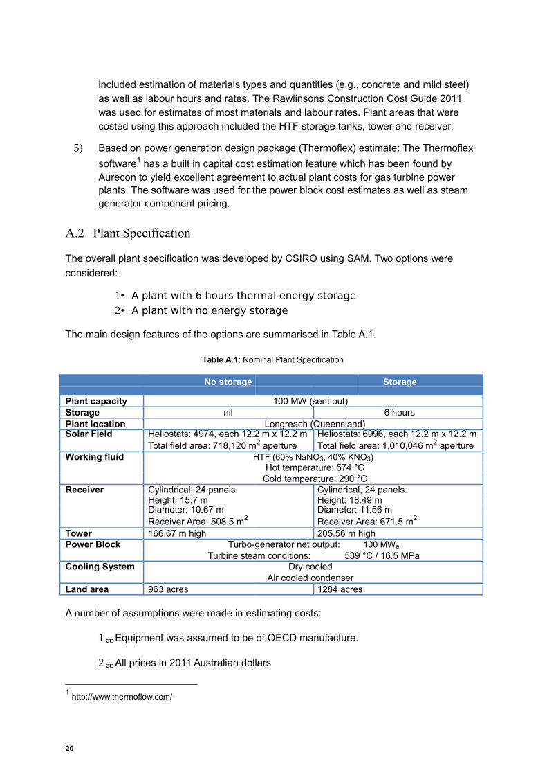
A.2 Plant Specification

The overall plant specification was developed by CSIRO using SAM. Two options were

considered:

1• A plant with 6 hours thermal energy storage

2• A plant with no energy storage

The main design features of the options are summarised in Table A.1.

Table A.1: Nominal Plant Specification

No storage Storage

Plant capacity 100 MW (sent out)Storage nil 6 hoursPlant location Longreach (Queensland)Solar Field Heliostats: 4974, each 12.2 m x 12.2 m Heliostats: 6996, each 12.2 m x 12.2 m

Total field area: 718,120 m2 aperture Total field area: 1,010,046 m2 apertureWorking fluid HTF (60% NaNO3, 40% KNO3)

Hot temperature: 574 °CCold temperature: 290 °C

Receiver Cylindrical, 24 panels. Cylindrical, 24 panels.Height: 15.7 m Height: 18.49 mDiameter: 10.67 m Diameter: 11.56 mReceiver Area: 508.5 m2 Receiver Area: 671.5 m2

Tower 166.67 m high 205.56 m highPower Block Turbo-generator net output: 100 MWe

Turbine steam conditions: 539 °C / 16.5 MPaCooling System Dry cooled

Air cooled condenserLand area 963 acres 1284 acres

A number of assumptions were made in estimating costs:

1Equipment was assumed to be of OECD manufacture.

2All prices in 2011 Australian dollars

1 http://www.thermoflow.com/

20

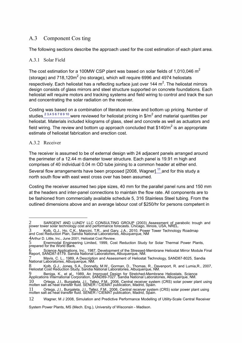
A.3 Component Cos ting

The following sections describe the approach used for the cost estimation of each plant area.

A.3.1 Solar Field

The cost estimation for a 100MW CSP plant was based on solar fields of 1,010,046 m2

(storage) and 718,120m2 (no storage), which will require 6996 and 4974 heliostats

respectively. Each heliostat has a reflecting surface just over 144 m2. The heliostat mirrors design consists of glass mirrors and steel structure supported on concrete foundations. Eachheliostat will require motors and tracking systems and field wiring to control and track the sunand concentrating the solar radiation on the receiver.

Costing was based on a combination of literature review and bottom up pricing. Number of

studies 2 3,4 5 6 7 8 9 10 were reviewed for heliostat pricing in $/m2 and material quantities per heliostat. Materials included kilograms of glass, steel and concrete as well as actuators andfield wiring. The review and bottom up approach concluded that $140/m2 is an appropriate estimate of heliostat fabrication and erection cost.

A.3.2 Receiver

The receiver is assumed to be of external design with 24 adjacent panels arranged around the perimeter of a 12.44 m diameter tower structure. Each panel is 19.91 m high and comprises of 40 individual 0.04 m OD tube joining to a common header at either end.

Several flow arrangements have been proposed [2008, Wagner] 11 and for this study a north south flow with east west cross over has been assumed.

Costing the receiver assumed two pipe sizes, 40 mm for the parallel panel runs and 150 mmat the headers and inter-panel connections to maintain the flow rate. All components are to be fashioned from commercially available schedule 5, 316 Stainless Steel tubing. From the outlined dimensions above and an average labour cost of $250/hr for persons competent in

2 SARGENT AND LUNDY LLC CONSULTING GROUP (2003) Assessment of parabolic trough andpower tower solar technology cost and performance forecasts. Chicago, Illinois, USA, NREL. 3 Kolb, G.J., Ho, C.K., Mancini, T.R., and Gary, J.A., 2010, Power Tower Technology Roadmapand Cost Reduction Plan, Sandia National Laboratories, Albuquerque, NM 4Arthur D. Little, Inc., June 2001, Heliostat Cost Review. 5 Enermodal Engineering Limited, 1999, Cost Reduction Study for Solar Thermal Power Plants,prepared for the World Bank. 6 Science Applications, Inc., 1987, Development of the Stressed-Membrane Heliostat Mirror Module FinalReport, SAND87-8179. Sandia National Laboratories, Albuquerque, NM. 7 Mavis, C. L., 1989, A Description and Assessment of Heliostat Technology, SAND87-8025, SandiaNational Laboratories, Albuquerque, NM. 8 Kolb, G.J., Jones, S.A., Donnelly, M.W., Gorman, D., Thomas, R., Davenport, R. and Lumia,R., 2007,Heliostat Cost Reduction Study, Sandia National Laboratories, Albuquerque, NM. 9 Beniga, K., et al., 1989, An Improved Design for Stretched-Membrane Heliostats, ScienceApplications International Corporation, SAND89-7027. Sandia National Laboratories, Albuquerque, NM. 10 Ortega, J.I., Burgaleta, J.I., Tellez, F.M., 2006, Central receiver system (CRS) solar power plant usingmolten salt as heat transfer fluid. SENER / CIEMAT publication, Madrid, Spain. 11 Ortega, J.I., Burgaleta, J.I., Tellez, F.M., 2006, Central receiver system (CRS) solar power plant usingmolten salt as heat transfer fluid. SENER / CIEMAT publication, Madrid, Spain.

12 Wagner, M J 2008, Simulation and Predictive Performance Modelling of Utility-Scale Central Receiver

System Power Plants, MS (Mech. Eng.), University of Wisconsin - Madison.

pressure welding, the cost of fabrication and installation has been determined as shown in

Table A.2.

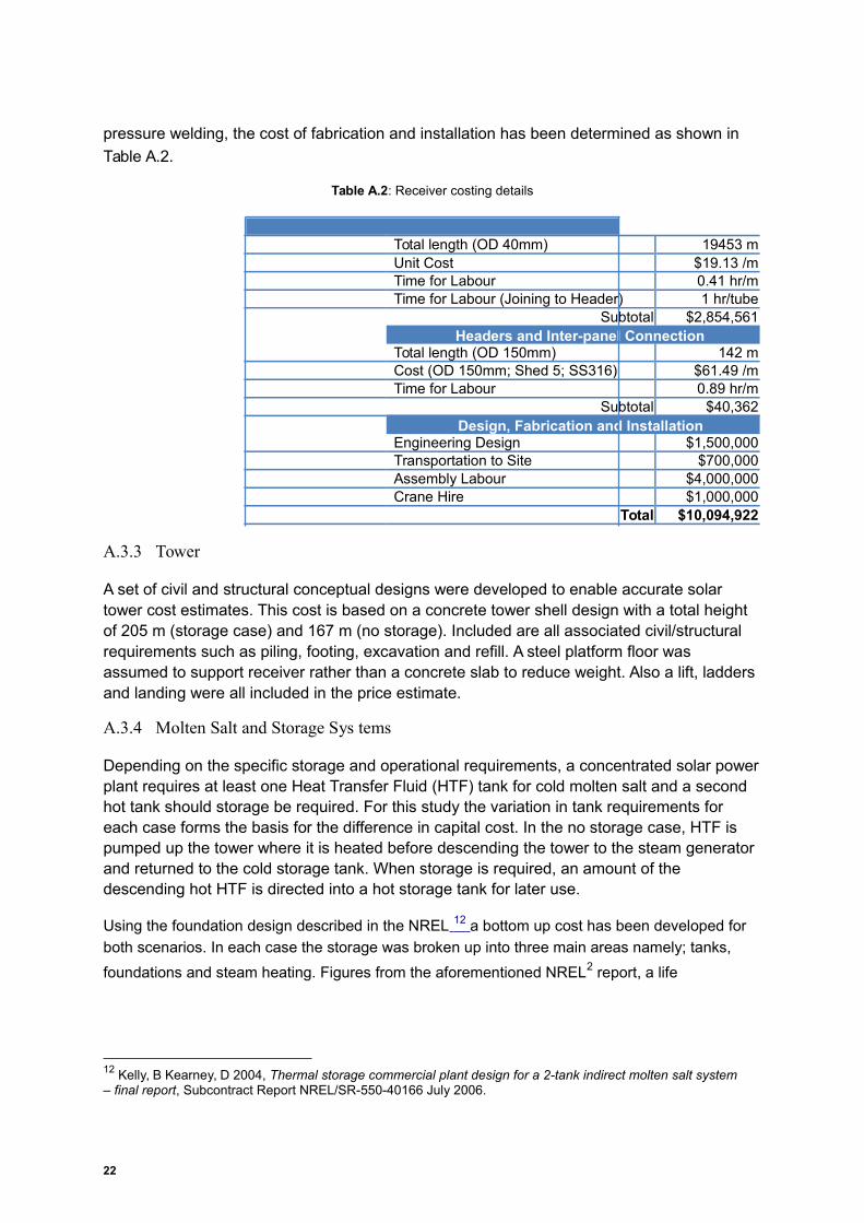
Table A.2: Receiver costing details

PanelsTotal length (OD 40mm) 19453 mUnit Cost $19.13 /mTime for Labour 0.41 hr/mTime for Labour (Joining to Header) 1 hr/tube

Subtotal $2,854,561Headers and Inter-panel Connection

Total length (OD 150mm) 142 mCost (OD 150mm; Shed 5; SS316) $61.49 /mTime for Labour 0.89 hr/m

Subtotal $40,362Design, Fabrication and Installation

Engineering Design $1,500,000Transportation to Site $700,000Assembly Labour $4,000,000Crane Hire $1,000,000

Total $10,094,922

A.3.3 Tower

A set of civil and structural conceptual designs were developed to enable accurate solar tower cost estimates. This cost is based on a concrete tower shell design with a total height of 205 m (storage case) and 167 m (no storage). Included are all associated civil/structural requirements such as piling, footing, excavation and refill. A steel platform floor was assumed to support receiver rather than a concrete slab to reduce weight. Also a lift, laddersand landing were all included in the price estimate.

A.3.4 Molten Salt and Storage Sys tems

Depending on the specific storage and operational requirements, a concentrated solar powerplant requires at least one Heat Transfer Fluid (HTF) tank for cold molten salt and a second hot tank should storage be required. For this study the variation in tank requirements for each case forms the basis for the difference in capital cost. In the no storage case, HTF is pumped up the tower where it is heated before descending the tower to the steam generatorand returned to the cold storage tank. When storage is required, an amount of the descending hot HTF is directed into a hot storage tank for later use.

Using the foundation design described in the NREL 12 a bottom up cost has been developed for

both scenarios. In each case the storage was broken up into three main areas namely; tanks,

foundations and steam heating. Figures from the aforementioned NREL2 report, a life

12 Kelly, B Kearney, D 2004, Thermal storage commercial plant design for a 2-tank indirect molten salt system – final report, Subcontract Report NREL/SR-550-40166 July 2006.

22

cycle assessment of thermal storage 13 and internal experience with the Australian

construction industry have been combined to formulate this capital cost estimate.

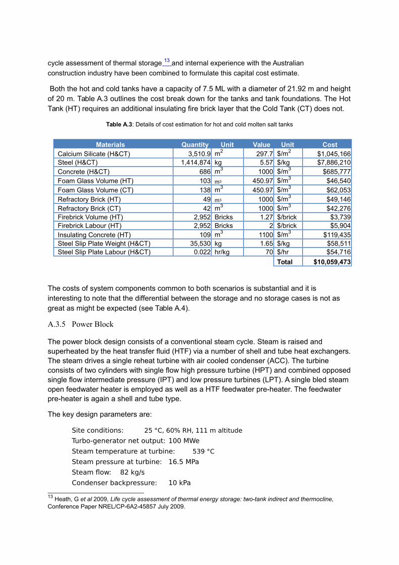
Both the hot and cold tanks have a capacity of 7.5 ML with a diameter of 21.92 m and heightof 20 m. Table A.3 outlines the cost break down for the tanks and tank foundations. The HotTank (HT) requires an additional insulating fire brick layer that the Cold Tank (CT) does not.

Table A.3: Details of cost estimation for hot and cold molten salt tanks

Materials Quantity Unit Value Unit CostCalcium Silicate (H&CT) 3,510.9 m2 297.7 $/m2 $1,045,166Steel (H&CT) 1,414,874 kg 5.57 $/kg $7,886,210Concrete (H&CT) 686 m3 1000 $/m3 $685,777Foam Glass Volume (HT) 103 m3 450.97 $/m3 $46,540Foam Glass Volume (CT) 138 m3 450.97 $/m3 $62,053Refractory Brick (HT) 49 m3 1000 $/m3 $49,146Refractory Brick (CT) 42 m3 1000 $/m3 $42,276Firebrick Volume (HT) 2,952 Bricks 1.27 $/brick $3,739Firebrick Labour (HT) 2,952 Bricks 2 $/brick $5,904Insulating Concrete (HT) 109 m3 1100 $/m3 $119,435Steel Slip Plate Weight (H&CT) 35,530 kg 1.65 $/kg $58,511Steel Slip Plate Labour (H&CT) 0.022 hr/kg 70 $/hr $54,716

Total $10,059,473

The costs of system components common to both scenarios is substantial and it is interesting to note that the differential between the storage and no storage cases is not asgreat as might be expected (see Table A.4).

A.3.5 Power Block

The power block design consists of a conventional steam cycle. Steam is raised and superheated by the heat transfer fluid (HTF) via a number of shell and tube heat exchangers.The steam drives a single reheat turbine with air cooled condenser (ACC). The turbine consists of two cylinders with single flow high pressure turbine (HPT) and combined opposedsingle flow intermediate pressure (IPT) and low pressure turbines (LPT). A single bled steam open feedwater heater is employed as well as a HTF feedwater pre-heater. The feedwater pre-heater is again a shell and tube type.

The key design parameters are:

Site conditions: 25 °C, 60% RH, 111 m altitude

Turbo-generator net output: 100 MWe

Steam temperature at turbine: 539 °C

Steam pressure at turbine: 16.5 MPa

Steam flow: 82 kg/s

Condenser backpressure: 10 kPa

13 Heath, G et al 2009, Life cycle assessment of thermal energy storage: two-tank indirect and thermocline,Conference Paper NREL/CP-6A2-45857 July 2009.

A model of the above configuration was created with Thermoflex Version 20 which is a thermodynamic modelling package by Thermoflow. Based on the model outcomes additionalshell and tube heat exchangers were included to stage the pre-heating, superheating and reheating. To reduce vessel size parallel paths were used for the pre-heaters, evaporators and superheaters.

Although the original design criteria called for a condenser backpressure of 4.2 kPa (1.25 in Hg) it was found that the ACC would need to be significantly larger without appreciable performance benefit. Initial indications are that towards the lower end of possible backpressures, additional heliostats may be more cost effective than additional ACC cells asa strategy to increase net electrical output for a given steam condition, flow and turbine. As well as ACC size and cost increasing as backpressure required decreases, so to does the auxiliary energy required for ACC fans.

The Thermoflex library of heat transfer fluids includes the nitrate salt 60% NaNO3/40%

KNO3 thus making correct modelling of heat transfer and heat exchanger design possible.

Thermoflex provides cost estimates for certain components including the turbine, shell and tube heat exchangers and ACC. The current version cost estimates are as of December 2009. In 2009 Aurecon compared Thermoflow GTPro cost estimates against actual costs fortwo power plants built in Australia and found good correlation. The power plants were both gas fired, one open cycle and the other combined cycle.

A.3.6 Other project cos ts

In addition to the plant equipment costs described above, there are other costs that are not attributable to particular items of equipment, but are incurred by the owner during the periodbetween project development to financial close and the period of construction. These costs or allowances include: contingency on high risk items, permits, licenses and fees, miscellaneous, bonds, insurance, legal & financial, escalation & interest during construction,project administration and developers’ fee. For a solar thermal project, both engineering anddevelopment costs may be expected to be higher than for fossil plants (at least during the early stages of technology uptake). Land procurement is also a cost to the owner that must be considered. Based on GTPRO estimated owner costs for a combined cycle plant project,an allowance of 30% has been included for ‘other project costs’.

24

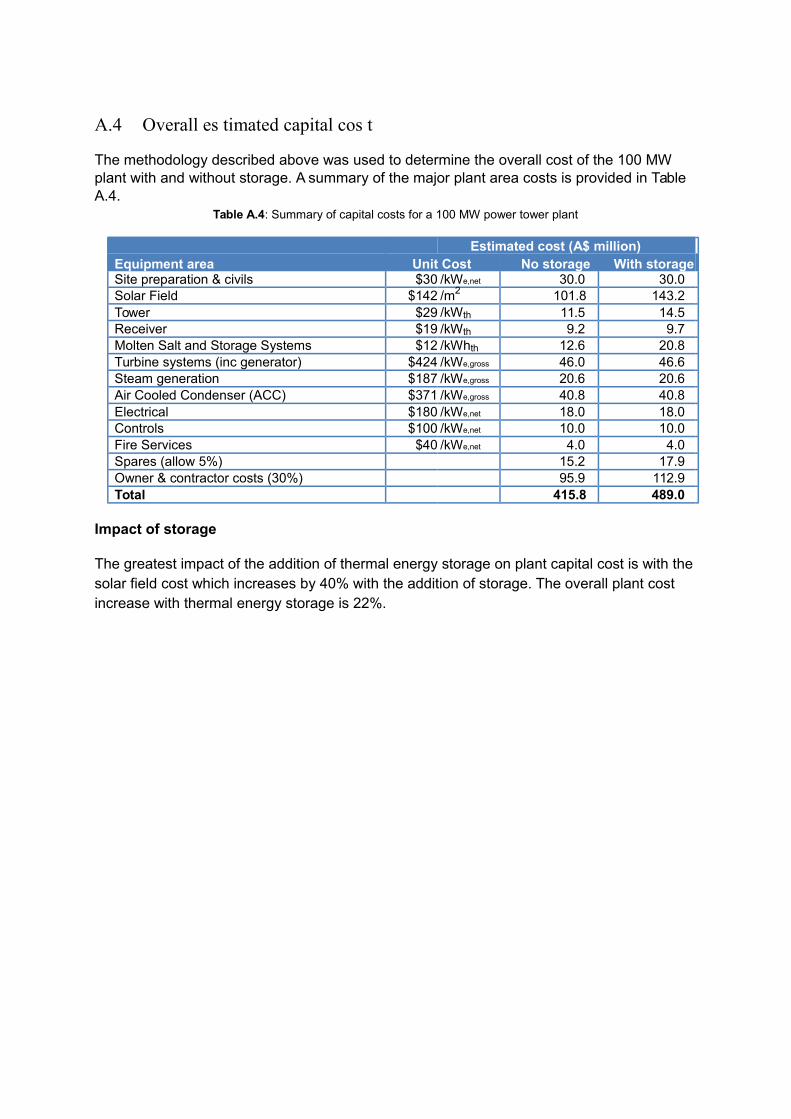
A.4 Overall es timated capital cos t

The methodology described above was used to determine the overall cost of the 100 MW plant with and without storage. A summary of the major plant area costs is provided in TableA.4.

Table A.4: Summary of capital costs for a 100 MW power tower plant

Estimated cost (A$ million)Equipment area Unit Cost No storage With storageSite preparation & civils $30 /kWe,net 30.0 30.0Solar Field $142 /m2 101.8 143.2Tower $29 /kWth 11.5 14.5Receiver $19 /kWth 9.2 9.7Molten Salt and Storage Systems $12 /kWhth 12.6 20.8Turbine systems (inc generator) $424 /kWe,gross 46.0 46.6Steam generation $187 /kWe,gross 20.6 20.6Air Cooled Condenser (ACC) $371 /kWe,gross 40.8 40.8Electrical $180 /kWe,net 18.0 18.0Controls $100 /kWe,net 10.0 10.0Fire Services $40 /kWe,net 4.0 4.0Spares (allow 5%) 15.2 17.9Owner & contractor costs (30%) 95.9 112.9Total 415.8 489.0

Impact of storage

The greatest impact of the addition of thermal energy storage on plant capital cost is with thesolar field cost which increases by 40% with the addition of storage. The overall plant cost increase with thermal energy storage is 22%.

APPENDIX B: THERMODYNAMIC EXPLANATION OF RANKINE STEAM CYCLES

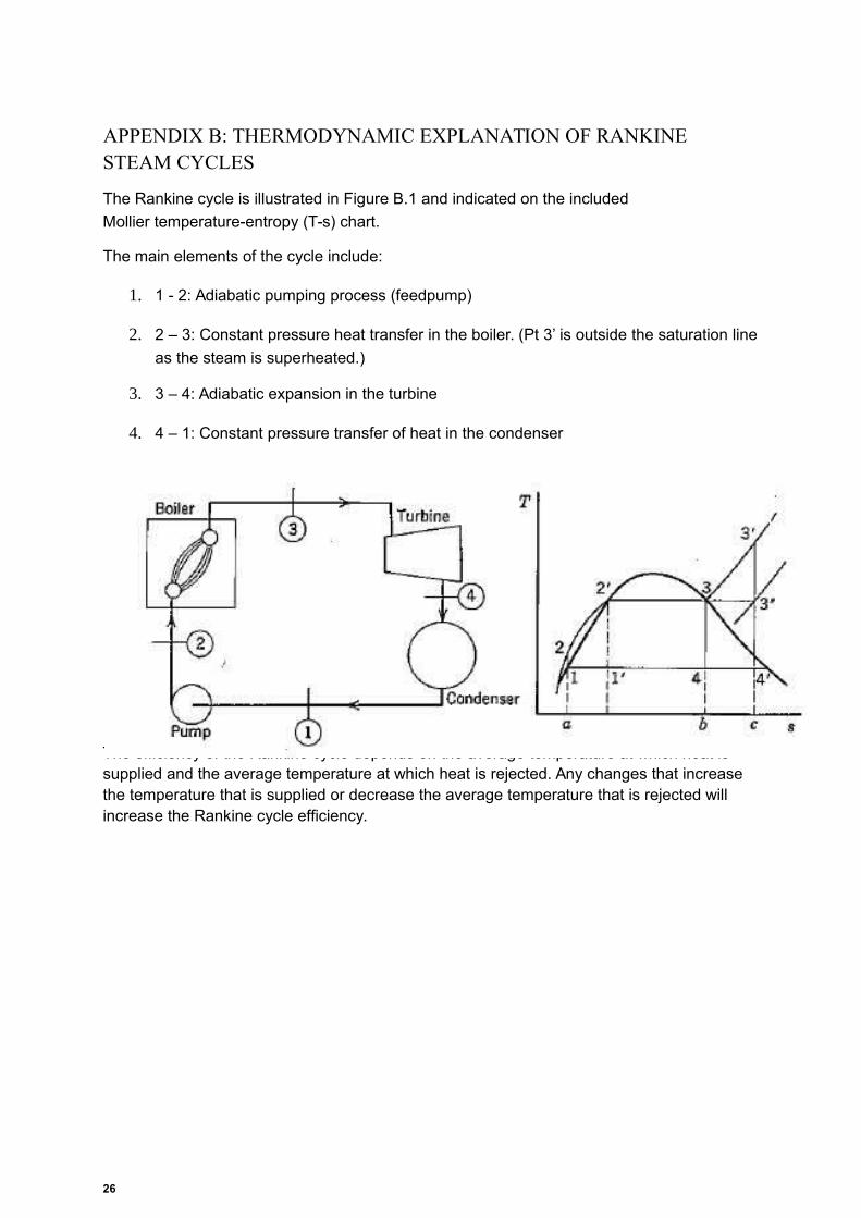
The Rankine cycle is illustrated in Figure B.1 and indicated on the included

Mollier temperature-entropy (T-s) chart.

The main elements of the cycle include:

1. 1 - 2: Adiabatic pumping process (feedpump)

2. 2 – 3: Constant pressure heat transfer in the boiler. (Pt 3’ is outside the saturation line

as the steam is superheated.)

3. 3 – 4: Adiabatic expansion in the turbine

4. 4 – 1: Constant pressure transfer of heat in the condenser

Figure B.1: Simple Rankine steam cycle power plant (Van Wylen & Sonntag, 1976)

The efficiency of the Rankine cycle depends on the average temperature at which heat is supplied and the average temperature at which heat is rejected. Any changes that increasethe temperature that is supplied or decrease the average temperature that is rejected will increase the Rankine cycle efficiency.

26