Constraining Recovery Observations for Trans‐Neptunian Objects with Poorly Known Orbits

Constraining Recovery Observations for Trans‐Neptunian Objects with Poorly Known OrbitsAuthor(s): Jeffrey D. Goldader and Charles AlcockSource: Publications of the Astronomical Society of the Pacific, Vol. 115, No. 813 (November2003), pp. 1330-1339Published by: The University of Chicago Press on behalf of the Astronomical Society of the PacificStable URL: http://www.jstor.org/stable/10.1086/379218 .

Accessed: 25/05/2014 01:31

Your use of the JSTOR archive indicates your acceptance of the Terms & Conditions of Use, available at .http://www.jstor.org/page/info/about/policies/terms.jsp

.JSTOR is a not-for-profit service that helps scholars, researchers, and students discover, use, and build upon a wide range ofcontent in a trusted digital archive. We use information technology and tools to increase productivity and facilitate new formsof scholarship. For more information about JSTOR, please contact [email protected].

.

The University of Chicago Press and Astronomical Society of the Pacific are collaborating with JSTOR todigitize, preserve and extend access to Publications of the Astronomical Society of the Pacific.

http://www.jstor.org

This content downloaded from 195.78.108.118 on Sun, 25 May 2014 01:31:33 AMAll use subject to JSTOR Terms and Conditions

http://www.jstor.org/action/showPublisher?publisherCode=ucpress

http://www.jstor.org/action/showPublisher?publisherCode=astrosocpac

http://www.jstor.org/stable/10.1086/379218?origin=JSTOR-pdf

http://www.jstor.org/page/info/about/policies/terms.jsp


1330

Publications of the Astronomical Society of the Pacific, 115:1330–1339, 2003 November� 2003. The Astronomical Society of the Pacific. All rights reserved. Printed in U.S.A.

Constraining Recovery Observations for Trans-Neptunian Objectswith Poorly Known Orbits

Jeffrey D. Goldader and Charles Alcock

Department of Physics and Astronomy, University of Pennsylvania, 209 South 33rd Street, Philadelphia, PA 19104;[email protected], [email protected]

Received 2003 June 9; accepted 2003 August 22

ABSTRACT. We present a simple method for constraining the possible future positions of distant solar systemobjects observed twice over only a very short time span. The method involves taking two positions and thendetermining a large number of possible orbits compatible with the observed motion across the sky for an objectwith unknown (but constrainable) distance from Earth. A key advantage of this approach is that it assumes onlythat the object is bound and distant. Monte Carlo techniques are used to incorporate astrometric uncertainty andmap out the allowed orbital parameter space. The method allows us to compute the object’s position on theselected recovery date for each potential orbit, assisting the selection of fields for recovery observations. Examplesare shown, and usage of the code is discussed.

1. INTRODUCTION

The problem of initial orbit determination of celestial objectsis centuries old. Marsden (1985, 1991) cites references goingback more than 200 years and reviews modern applications ofGauss’s method. More recent efforts include those of Bernstein& Khushalani (2000) and Virtanen et al. (2001).

Reliable orbit determinations require several observations,because a proper orbit is described by six orbital parameters(semimajor axis, eccentricity, inclination, longitude of the as-cending node, argument of pericenter, and time of pericenterpassage). Since a simple observation of the celestial coordinatesof an object does not tell us the distance to the object, twosuch observations spaced closely in time are insufficient toyield a reliable orbit.

Circumstances sometimes unavoidably result in very fewobservations being taken of a newly discovered object, and thisis the case for our own Southern Edgeworth-Kuiper Surveyfor Trans-Neptunian Objects (TNOs), described by Marshall etal. (2001) and Moody et al. (2003). The survey took data atMount Stromlo for about 3 years. It used the MACHO telescopesystem to search large patches of sky (∼ ) for slowly0�.7# 0�.7moving objects that were possibly TNOs.

Fitting reliable orbits from our archive observations aloneis not possible. With the observing strategy of our survey, thearc of observations was short, and a TNO would be visible inat most three images, taken over a time span of at most1 week.1 As Bernstein & Khushalani (2000) discuss, only the

1 Typically, we would take two images of a field a few hours apart on onenight, both on the same side of the meridian, followed within the next fewnights by another single image of the same field.

inclination of the orbit and heliocentric distance can be con-strained with such a short arc, and even that assumes a circularorbit, with the inherent degeneracies in the remaining orbitalparameters. The longer between the discovery and recoveryobservations, the larger the area of sky that must be searched.We needed to find a way to use only our few observations topredict and constrain the position of a candidate at a laterapparition, so as to maximize the possibility of recovery whileminimizing the area of sky we would have to search to recoverthe object. Once recovered, a candidate’s orbit could be de-termined using one of the conventional methods (such as thoseused by the IAU Minor Planet Center or that of Bernstein &Khushalani 2000).

In the case of poorly constrained orbits, recovery observa-tions for distant moving objects become increasingly more dif-ficult and expensive (in terms of telescope time) as one movesfarther in time from the epoch of discovery. The instantaneousobserved motion of a TNO is primarily caused by the Earth’sown motion around the Sun. But a TNO in an orbit with semi-major axis of 40 AU would complete an orbit in about 250years. If the orbit were nearly circular, the TNO would moveat a nearly constant∼1�.44 across the celestial sphere over thecourse of a single year. In reality, most orbits are reasonablynoncircular, and so there may be significant acceleration in themotion of the TNO, even in arcs as short as 1 yr (e.g., theTNO 2000 CR105, discussed in Millis et al. 2002 and Gladmanet al. 2002).

This paper documents a method to better constrain the likelypositions of TNOs with short discovery arcs at some futureepoch, in order to enhance the probability of recovering theobjects. Our source code will be made publicly available



CONSTRAINING TNO RECOVERIES 1331

2003 PASP,115:1330–1339

Fig. 1.—Demonstration of the method, using Pluto “observations” on 2003June 1.0 and June 8.0 UT. The heliocentric equatorialX-Y plane is shown.The observed Earth-Pluto position vectors are drawn in; the dots are Pluto’sactual positions. At Pluto’s true distance from the Sun, the greatest distanceit could travel between the two observation times is shown as the circle centeredat the first position. The arrows show some possible motion vectors betweenthe two observations. Since the position vectors eventually cross, a second setof solutions at much greater heliocentric distance yields retrograde orbits. Asof this writing, no known TNO has a retrograde orbit.

on-line,2 and we hope to have a Web-enabled version of thecode by the time this article appears.

2. THE MODEL

We work in a Cartesian, heliocentric equatorial coordinatesystem. The model assumes that the TNO is in a bound orbit.Two observations (the first the discovery observation, and asecond observation that we assume is taken no more than1 week later) give us the vectors along which the TNO mustbe located, but not the distance to the TNO (see Fig. 1). Thefirst example we will give here is for Pluto, “observed” usingpositions calculated on 2003 June 1.0 UT and 2003 June 8.0UT. (Since Pluto’s orbit is known, we can find its celestial andthree-dimensional Cartesian coordinates at any time, and so itprovides a good example to check the method.)

Since Pluto is indeed a TNO, at “discovery,” it is located atsome great distance ( ), which we assume to be at least,dET1

say, 27 AU from the Earth.3 The Earth’s coordinates at thetimes of the first and second observations are ( , , ) andx y zE1 E1 E1

( , , ). Since the Earth’s orbit is well known and thex y zE2 E2 E2

coordinate system is well defined, simply specifying the datesof the observations allows the determination of the Earth’sthree-dimensional coordinates using routines fromslalib, apackage used extensively in this work (available on theInternet.4

We know only the projection of the TNO’s position on thecelestial sphere at the moment of the first observation, not itsthree-dimensional coordinates. Since the right ascension anddeclination are known, we can calculate the TNO’s geocentricequatorial coordinates relative to the unit vector. This gives usa vector with origin at Earth’s position at time 1 (T1), alongwhich the TNO must lie, with the form

ˆˆ ˆi i � j j � k k, (1)1 1 1

where , , and are the coefficients of the unit vectori j k1 1 1

( ). (We ignore diurnal aberration, which can2 2 2i � j � k p 11 1 1

cause offsets of�0�.2 in observed and geocentric coordinates;this introduces errors of magnitude similar to the astrometricuncertainty. The maximum error comes when the observationsare taken at opposite ends of the night; the error is minimizedwhen both observations are taken at the same clock time, par-

2 http://www.astro.upenn.edu/projects/TNO.3 The distance of 27 AU was chosen arbitrarily, but the intent was to favor

objects exterior to Neptune’s orbit. As shown in the numerical integrations byDuncan, Levison, & Budd (1995) and other authors, orbits with periheliondistances�35 AU are dynamically unstable on timescales of�108 yr, unlessthey are located in Neptune mean motion resonances. Holman & Wisdom(1993) found that orbits between Uranus and Neptune are unstable on time-scales of roughly�106 yr. Such objects are occasionally found as Centaurs,of which (2060) Chiron is the best known, whose orbits are temporarily locatedbetween those of Jupiter and Neptune. As we show later, however, our codedoes appear to work as intended for Centaurs.

4 http://star-www.rl.ac.uk/Software/software.htm.

ticularly near midnight. Our observing strategy was to obtainexposures on different nights at nearly the same clock time,reducing the error due to diurnal aberration.)

The vector for the first observation itself, now transformedto heliocentric by adding in Earth’s own coordinates, is givenin parametric form as

x p x � d i ,T E1 1 11

y p y � d j ,T E1 1 11

z p z � d k , (2)T E1 1 11

where the distance parameter at the origin of the vectord p 01

(i.e., at Earth) and increases away from Earth; at the trued1

geocentric distance of the TNO, .d p d1 ET1

The explicit assumption of the distance to the TNO at agiven time (say, setting the Earth-TNO distance at the timed1

of the first observation to 27 AU) allows us to identify oneunique possible location (in Cartesian geocentric equatorial co-ordinates) of the TNO along the vector.

We can construct the geocentric Earth-TNO vector at thesecond observation time in the same way. The position vectorfor the second observation is

ˆˆ ˆi i � j j � k k, (3)2 2 2



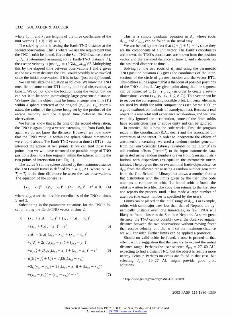
1332 GOLDADER & ALCOCK

2003 PASP,115:1330–1339

where , , and are lengths of the three coefficients of thei j k2 2 2

unit vector ( ).2 2 2i � j � k p 12 2 2

The sticking point is setting the Earth-TNO distance at thesecond observation. This is where we use the requirement thatthe TNO’s orbit be bound. Given the Sun-TNO distance at time1, (determined assuming some Earth-TNO distance ),d dST1 1

the escape velocity is just . Multiplying1/2v p (2GM /d )Sun ST1esc

this by the elapsed time between observations 1 and 2 givesus the maximum distance the TNO could possibly have traveledsince the initial observation, if it is in fact ( just barely) bound.

We can visualize the situation as follows. We know the TNOmust lie on some vectorET1 during the initial observation, attime 1. We do not know the location along the vector, but wecan set it to be some interestingly large geocentric distance.We know that the object must be found at some later time (T2)within a sphere centered at the original coordi-(x , y , z )T T T1 1 1

nates, the radius of the sphere being set by the product of theescape velocity and the elapsed time between the twoobservations.

We further know that at the time of the second observation,the TNO is again along a vector extending out from Earth, butagain we do not know the distance. However, we now knowthat the TNO must lie within the sphere whose dimensionswere found above. The Earth-TNO vector at time 2 (ET2) mustintersect the sphere at two points. If we can find those twopoints, then we will have narrowed the possible range of TNOpositions down to a line segment within the sphere, joining thetwo points of intersection (see Fig. 1).

The radius (r) of the sphere defined by the maximum distancethe TNO could travel is defined by , wherer p v DT DT pesc

is the time difference between the two observations.T � T2 1

The equation of the sphere is

2 2 2 2(x � x ) � (y � y ) � (z � z ) � r p 0, (4)T T T T T T2 1 2 1 2 1

wherex, y, z are the possible coordinates of the TNO at times1 and 2.

Substituting in the parametric equations for the TNO’s lo-cation along the Earth-TNO vector at time 2,

2 20 p (x � i d � x ) � (y � j d � y )E2 2 2 T E2 2 2 T1 1

2 2�(z � k d � z ) � r (5)E2 2 2 T1

2 2 2p i d � 2i d (x � x ) � (x � x )2 2 2 2 E2 T E2 T1 1

2 2 2�j d � 2j d (y � y ) � (y � y )2 2 2 2 E2 T E2 T1 1

2 2 2 2�k d � 2k d (z � z ) � (z � z ) � r (6)2 2 2 2 E2 T E2 T1 1

2 2 2 2p d (i � j � k ) � d [2i (x � x )2 2 2 2 2 2 E2 T1

2�2j (y � y ) � 2k (z � z )] � [(x � x )2 E2 T 2 E2 T E2 T1 1 1

2 2 2�(y � y ) � (z � z ) � r ]. (7)E2 T E2 T1 1

This is a simple quadratic equation in , whose rootsd2

and can be found in the usual way.d d2,low 2,high

We are helped by the fact that , since they2 2 2i � j � k p 12 2 2

are the components of a unit vector. The Earth’s coordinatesare known, the TNO’s coordinates are known from the positionvector and the assumed distance at time 1, andr depends onthe assumed distance at time 1.

Solving for the two roots of and using the parametricd2

TNO position equation (2) gives the coordinates of the inter-sections of the circle of greatest motion and the vectorET2.This defines a line segment that is the locus of possible positionsof the TNO at time 2. Any given point along that line segmentcan be connected to in order to create a seven-(x , y , z )T T T1 1 1

dimensional vector . This vector can be˙ ˙ ˙(x , y , z , x, y, z, T )T T T 11 1 1

to recover the corresponding possible orbit. Universal elementsare used byslalib for orbit computations (see Sterne 1960 ora good textbook on methods of astrodynamics). Because a realobject in a real orbit will experience acceleration, and we haveexplicitly ignored the acceleration, some of the fitted orbitshave eccentricities near or above unity and can be ignored.

In practice, this is how the code works. First, the programreads in the coordinates (R.A., decl.) and the associated un-certainties of the target. In order to incorporate the effects ofastrometric uncertainty, we used a random number generatorfrom the Gnu Scientific Library (available on the Internet5) toadd random offsets (“errors”) to the input astrometric data,generated using random numbers drawn from Gaussian distri-butions with dispersions (j) equal to the astrometric uncer-tainties. The program then draws an initial Earth-object distance

from the allowed range using a random number generatordET1

from the Gnu Scientific Library that draws a number from aflat distribution with the limits given by the user. The codeattempts to compute an orbit. If a bound orbit is found, theorbit is written to a file. The code then returns to the first stepand repeats the process, until it has made a large number ofattempts (the exact number is specified by the user).

Limits can be placed on the initial range of . For example,dET1

orbits with semimajor axes less than that of Neptune are dy-namically unstable over long timescales, so few TNOs willlikely be found closer to the Sun than Neptune. At some greatdistance, the TNO cannot possibly cover the observed angulardistance between the two observations without moving fasterthan escape velocity, and that will set the maximum distancewe will consider. Further limits can be applied a posteriori.

Should no valid orbits be found, a note is printed to thateffect, with a suggestion that the user try to expand the initialdistance range. Perhaps the user selected AU,d p 27–60ET1

expecting to find a distant TNO, but the object is really a morenearby Centaur. Perhaps no orbits are found in that case, butselecting AU might provide good orbitd p 10–27ET1

solutions.

5 http://www.gnu.org/directory/GNU/GNUsl.html.




2003 PASP,115:1330–1339

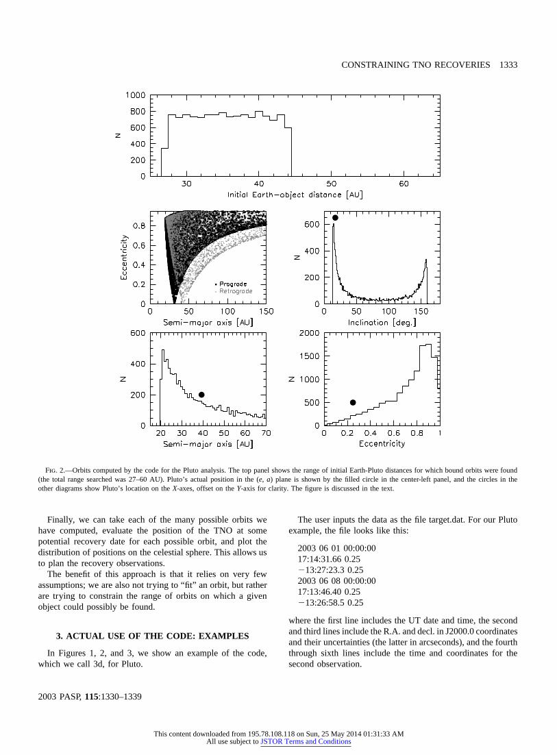
Fig. 2.—Orbits computed by the code for the Pluto analysis. The top panel shows the range of initial Earth-Pluto distances for which bound orbits were found(the total range searched was 27–60 AU). Pluto’s actual position in the plane is shown by the filled circle in the center-left panel, and the circles in the(e, a)other diagrams show Pluto’s location on theX-axes, offset on theY-axis for clarity. The figure is discussed in the text.

Finally, we can take each of the many possible orbits wehave computed, evaluate the position of the TNO at somepotential recovery date for each possible orbit, and plot thedistribution of positions on the celestial sphere. This allows usto plan the recovery observations.

The benefit of this approach is that it relies on very fewassumptions; we are also not trying to “fit” an orbit, but ratherare trying to constrain the range of orbits on which a givenobject could possibly be found.

3. ACTUAL USE OF THE CODE: EXAMPLES

In Figures 1, 2, and 3, we show an example of the code,which we call 3d, for Pluto.

The user inputs the data as the file target.dat. For our Plutoexample, the file looks like this:

2003 06 01 00:00:0017:14:31.66 0.25�13:27:23.3 0.252003 06 08 00:00:0017:13:46.40 0.25�13:26:58.5 0.25

where the first line includes the UT date and time, the secondand third lines include the R.A. and decl. in J2000.0 coordinatesand their uncertainties (the latter in arcseconds), and the fourththrough sixth lines include the time and coordinates for thesecond observation.




2003 PASP,115:1330–1339

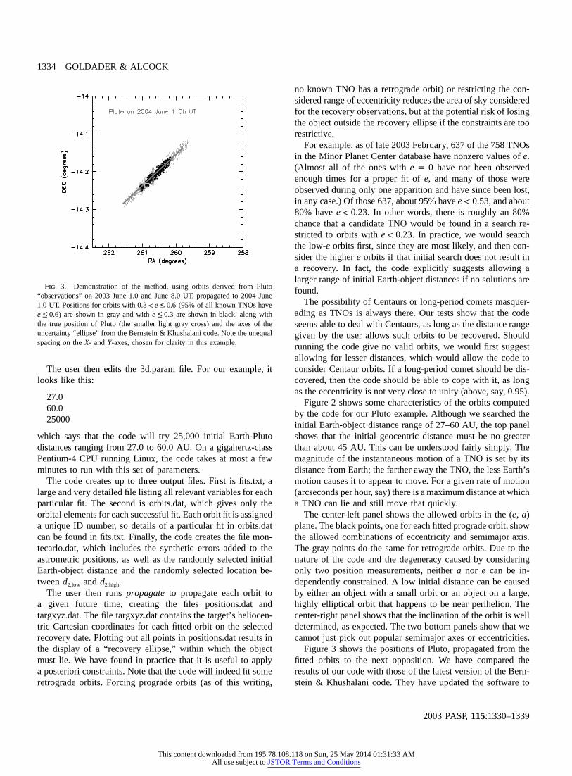
Fig. 3.—Demonstration of the method, using orbits derived from Pluto“observations” on 2003 June 1.0 and June 8.0 UT, propagated to 2004 June1.0 UT. Positions for orbits with (95% of all known TNOs have0.3! e ≤ 0.6

) are shown in gray and with are shown in black, along withe ≤ 0.6 e ≤ 0.3the true position of Pluto (the smaller light gray cross) and the axes of theuncertainty “ellipse” from the Bernstein & Khushalani code. Note the unequalspacing on theX- andY-axes, chosen for clarity in this example.

The user then edits the 3d.param file. For our example, itlooks like this:

27.060.025000

which says that the code will try 25,000 initial Earth-Plutodistances ranging from 27.0 to 60.0 AU. On a gigahertz-classPentium-4 CPU running Linux, the code takes at most a fewminutes to run with this set of parameters.

The code creates up to three output files. First is fits.txt, alarge and very detailed file listing all relevant variables for eachparticular fit. The second is orbits.dat, which gives only theorbital elements for each successful fit. Each orbit fit is assigneda unique ID number, so details of a particular fit in orbits.datcan be found in fits.txt. Finally, the code creates the file mon-tecarlo.dat, which includes the synthetic errors added to theastrometric positions, as well as the randomly selected initialEarth-object distance and the randomly selected location be-tweend2,low andd2,high.

The user then runspropagateto propagate each orbit toa given future time, creating the files positions.dat andtargxyz.dat. The file targxyz.dat contains the target’s heliocen-tric Cartesian coordinates for each fitted orbit on the selectedrecovery date. Plotting out all points in positions.dat results inthe display of a “recovery ellipse,” within which the objectmust lie. We have found in practice that it is useful to applya posteriori constraints. Note that the code will indeed fit someretrograde orbits. Forcing prograde orbits (as of this writing,

no known TNO has a retrograde orbit) or restricting the con-sidered range of eccentricity reduces the area of sky consideredfor the recovery observations, but at the potential risk of losingthe object outside the recovery ellipse if the constraints are toorestrictive.

For example, as of late 2003 February, 637 of the 758 TNOsin the Minor Planet Center database have nonzero values ofe.(Almost all of the ones with have not been observede p 0enough times for a proper fit ofe, and many of those wereobserved during only one apparition and have since been lost,in any case.) Of those 637, about 95% have , and aboute ! 0.5380% have . In other words, there is roughly an 80%e ! 0.23chance that a candidate TNO would be found in a search re-stricted to orbits with . In practice, we would searche ! 0.23the low-e orbits first, since they are most likely, and then con-sider the highere orbits if that initial search does not result ina recovery. In fact, the code explicitly suggests allowing alarger range of initial Earth-object distances if no solutions arefound.

The possibility of Centaurs or long-period comets masquer-ading as TNOs is always there. Our tests show that the codeseems able to deal with Centaurs, as long as the distance rangegiven by the user allows such orbits to be recovered. Shouldrunning the code give no valid orbits, we would first suggestallowing for lesser distances, which would allow the code toconsider Centaur orbits. If a long-period comet should be dis-covered, then the code should be able to cope with it, as longas the eccentricity is not very close to unity (above, say, 0.95).

Figure 2 shows some characteristics of the orbits computedby the code for our Pluto example. Although we searched theinitial Earth-object distance range of 27–60 AU, the top panelshows that the initial geocentric distance must be no greaterthan about 45 AU. This can be understood fairly simply. Themagnitude of the instantaneous motion of a TNO is set by itsdistance from Earth; the farther away the TNO, the less Earth’smotion causes it to appear to move. For a given rate of motion(arcseconds per hour, say) there is a maximum distance at whicha TNO can lie and still move that quickly.

The center-left panel shows the allowed orbits in the (e, a)plane. The black points, one for each fitted prograde orbit, showthe allowed combinations of eccentricity and semimajor axis.The gray points do the same for retrograde orbits. Due to thenature of the code and the degeneracy caused by consideringonly two position measurements, neithera nor e can be in-dependently constrained. A low initial distance can be causedby either an object with a small orbit or an object on a large,highly elliptical orbit that happens to be near perihelion. Thecenter-right panel shows that the inclination of the orbit is welldetermined, as expected. The two bottom panels show that wecannot just pick out popular semimajor axes or eccentricities.

Figure 3 shows the positions of Pluto, propagated from thefitted orbits to the next opposition. We have compared theresults of our code with those of the latest version of the Bern-stein & Khushalani code. They have updated the software to




2003 PASP,115:1330–1339

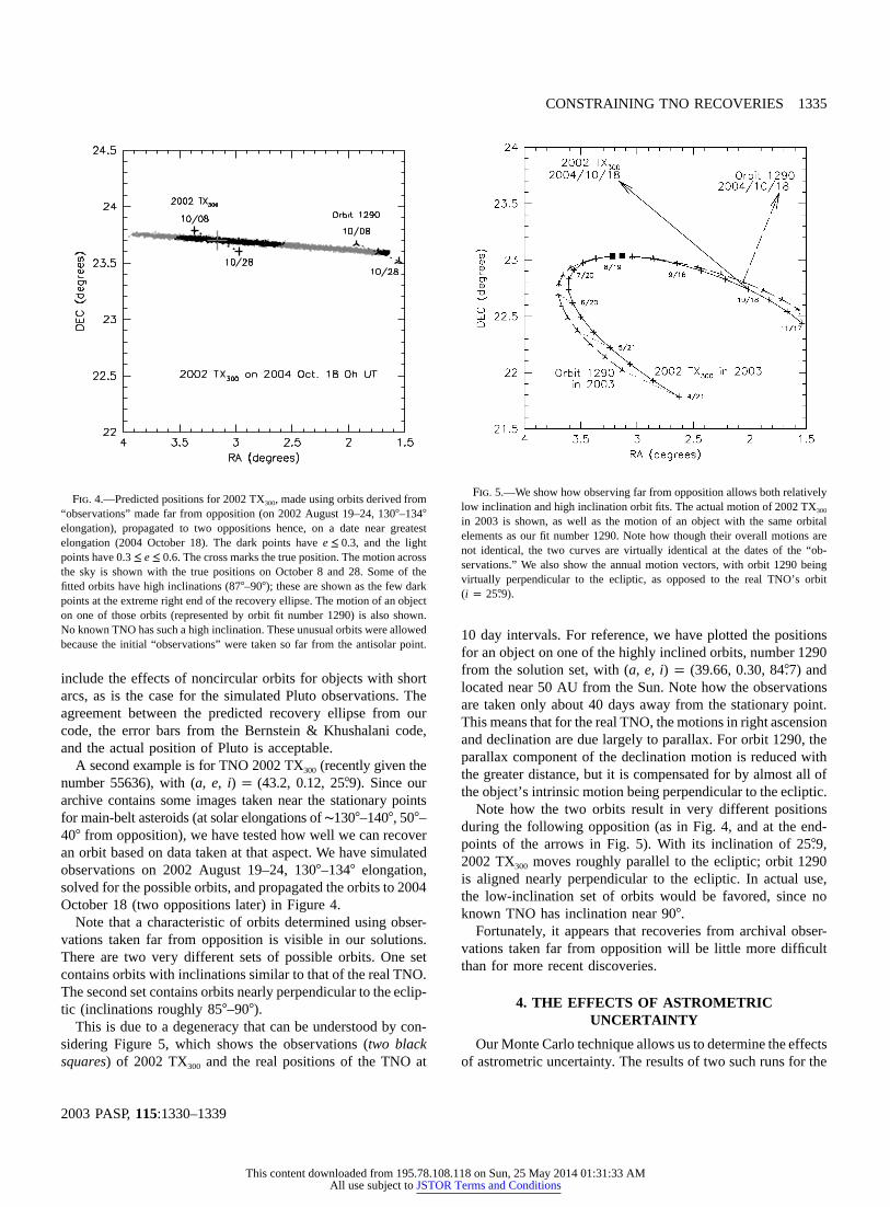
Fig. 4.—Predicted positions for 2002 TX300, made using orbits derived from“observations” made far from opposition (on 2002 August 19–24, 130�–134�elongation), propagated to two oppositions hence, on a date near greatestelongation (2004 October 18). The dark points have , and the lighte ≤ 0.3points have . The cross marks the true position. The motion across0.3≤ e ≤ 0.6the sky is shown with the true positions on October 8 and 28. Some of thefitted orbits have high inclinations (87�–90�); these are shown as the few darkpoints at the extreme right end of the recovery ellipse. The motion of an objecton one of those orbits (represented by orbit fit number 1290) is also shown.No known TNO has such a high inclination. These unusual orbits were allowedbecause the initial “observations” were taken so far from the antisolar point.

Fig. 5.—We show how observing far from opposition allows both relativelylow inclination and high inclination orbit fits. The actual motion of 2002 TX300

in 2003 is shown, as well as the motion of an object with the same orbitalelements as our fit number 1290. Note how though their overall motions arenot identical, the two curves are virtually identical at the dates of the “ob-servations.” We also show the annual motion vectors, with orbit 1290 beingvirtually perpendicular to the ecliptic, as opposed to the real TNO’s orbit( ).i p 25�.9

include the effects of noncircular orbits for objects with shortarcs, as is the case for the simulated Pluto observations. Theagreement between the predicted recovery ellipse from ourcode, the error bars from the Bernstein & Khushalani code,and the actual position of Pluto is acceptable.

A second example is for TNO 2002 TX300 (recently given thenumber 55636), with (a, e, i) p (43.2, 0.12, 25�.9). Since ourarchive contains some images taken near the stationary pointsfor main-belt asteroids (at solar elongations of∼130�–140�, 50�–40� from opposition), we have tested how well we can recoveran orbit based on data taken at that aspect. We have simulatedobservations on 2002 August 19–24, 130�–134� elongation,solved for the possible orbits, and propagated the orbits to 2004October 18 (two oppositions later) in Figure 4.

Note that a characteristic of orbits determined using obser-vations taken far from opposition is visible in our solutions.There are two very different sets of possible orbits. One setcontains orbits with inclinations similar to that of the real TNO.The second set contains orbits nearly perpendicular to the eclip-tic (inclinations roughly 85�–90�).

This is due to a degeneracy that can be understood by con-sidering Figure 5, which shows the observations (two blacksquares) of 2002 TX300 and the real positions of the TNO at

10 day intervals. For reference, we have plotted the positionsfor an object on one of the highly inclined orbits, number 1290from the solution set, with (a, e, i) p (39.66, 0.30, 84�.7) andlocated near 50 AU from the Sun. Note how the observationsare taken only about 40 days away from the stationary point.This means that for the real TNO, the motions in right ascensionand declination are due largely to parallax. For orbit 1290, theparallax component of the declination motion is reduced withthe greater distance, but it is compensated for by almost all ofthe object’s intrinsic motion being perpendicular to the ecliptic.

Note how the two orbits result in very different positionsduring the following opposition (as in Fig. 4, and at the end-points of the arrows in Fig. 5). With its inclination of 25�.9,2002 TX300 moves roughly parallel to the ecliptic; orbit 1290is aligned nearly perpendicular to the ecliptic. In actual use,the low-inclination set of orbits would be favored, since noknown TNO has inclination near 90�.

Fortunately, it appears that recoveries from archival obser-vations taken far from opposition will be little more difficultthan for more recent discoveries.

4. THE EFFECTS OF ASTROMETRICUNCERTAINTY

Our Monte Carlo technique allows us to determine the effectsof astrometric uncertainty. The results of two such runs for the




2003 PASP,115:1330–1339

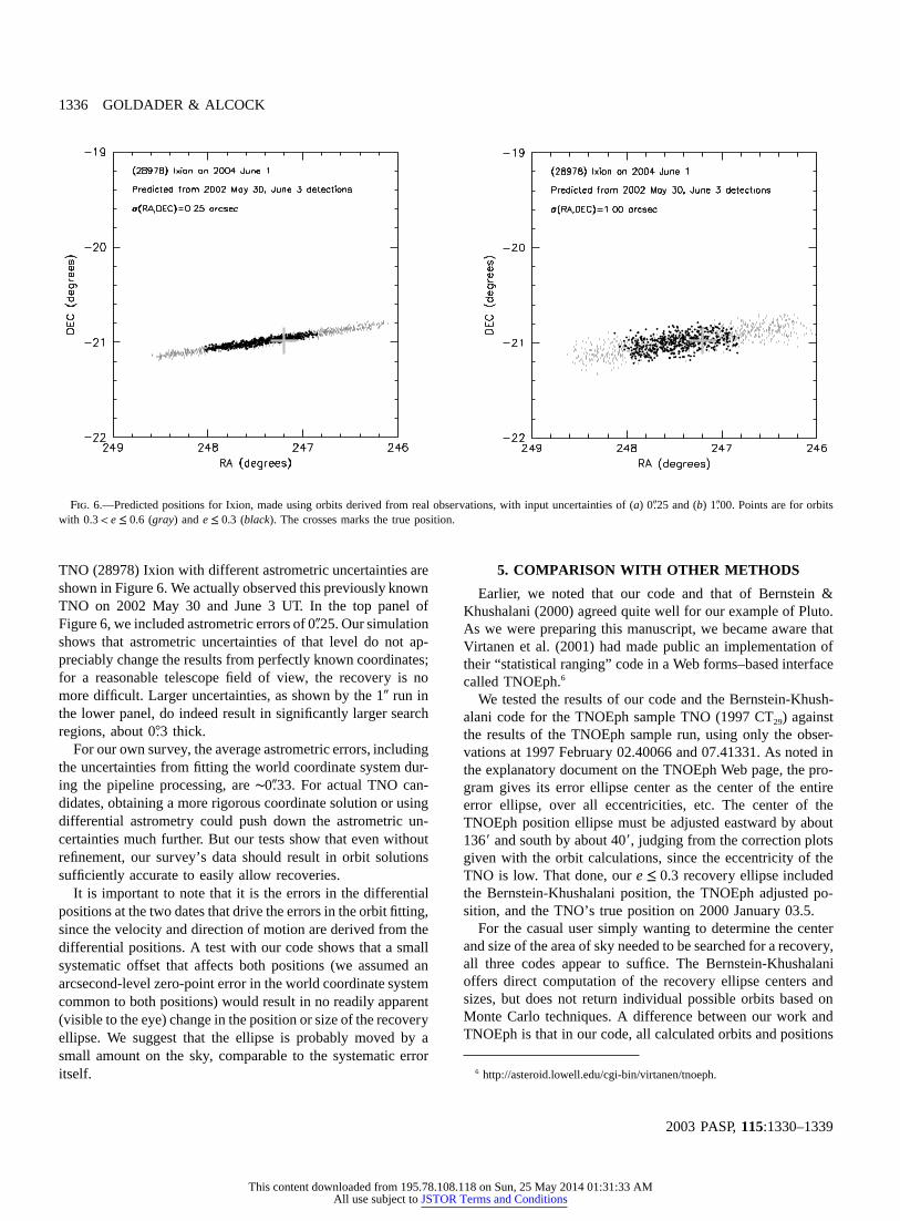
Fig. 6.—Predicted positions for Ixion, made using orbits derived from real observations, with input uncertainties of (a) 0�.25 and (b) 1�.00. Points are for orbitswith (gray) and (black). The crosses marks the true position.0.3! e ≤ 0.6 e ≤ 0.3

TNO (28978) Ixion with different astrometric uncertainties areshown in Figure 6. We actually observed this previously knownTNO on 2002 May 30 and June 3 UT. In the top panel ofFigure 6, we included astrometric errors of 0�.25. Our simulationshows that astrometric uncertainties of that level do not ap-preciably change the results from perfectly known coordinates;for a reasonable telescope field of view, the recovery is nomore difficult. Larger uncertainties, as shown by the 1� run inthe lower panel, do indeed result in significantly larger searchregions, about 0�.3 thick.

For our own survey, the average astrometric errors, includingthe uncertainties from fitting the world coordinate system dur-ing the pipeline processing, are∼0�.33. For actual TNO can-didates, obtaining a more rigorous coordinate solution or usingdifferential astrometry could push down the astrometric un-certainties much further. But our tests show that even withoutrefinement, our survey’s data should result in orbit solutionssufficiently accurate to easily allow recoveries.

It is important to note that it is the errors in the differentialpositions at the two dates that drive the errors in the orbit fitting,since the velocity and direction of motion are derived from thedifferential positions. A test with our code shows that a smallsystematic offset that affects both positions (we assumed anarcsecond-level zero-point error in the world coordinate systemcommon to both positions) would result in no readily apparent(visible to the eye) change in the position or size of the recoveryellipse. We suggest that the ellipse is probably moved by asmall amount on the sky, comparable to the systematic erroritself.

5. COMPARISON WITH OTHER METHODS

Earlier, we noted that our code and that of Bernstein &Khushalani (2000) agreed quite well for our example of Pluto.As we were preparing this manuscript, we became aware thatVirtanen et al. (2001) had made public an implementation oftheir “statistical ranging” code in a Web forms–based interfacecalled TNOEph.6

We tested the results of our code and the Bernstein-Khush-alani code for the TNOEph sample TNO (1997 CT29) againstthe results of the TNOEph sample run, using only the obser-vations at 1997 February 02.40066 and 07.41331. As noted inthe explanatory document on the TNOEph Web page, the pro-gram gives its error ellipse center as the center of the entireerror ellipse, over all eccentricities, etc. The center of theTNOEph position ellipse must be adjusted eastward by about136� and south by about 40�, judging from the correction plotsgiven with the orbit calculations, since the eccentricity of theTNO is low. That done, our recovery ellipse includede ≤ 0.3the Bernstein-Khushalani position, the TNOEph adjusted po-sition, and the TNO’s true position on 2000 January 03.5.

For the casual user simply wanting to determine the centerand size of the area of sky needed to be searched for a recovery,all three codes appear to suffice. The Bernstein-Khushalanioffers direct computation of the recovery ellipse centers andsizes, but does not return individual possible orbits based onMonte Carlo techniques. A difference between our work andTNOEph is that in our code, all calculated orbits and positions

6 http://asteroid.lowell.edu/cgi-bin/virtanen/tnoeph.




2003 PASP,115:1330–1339

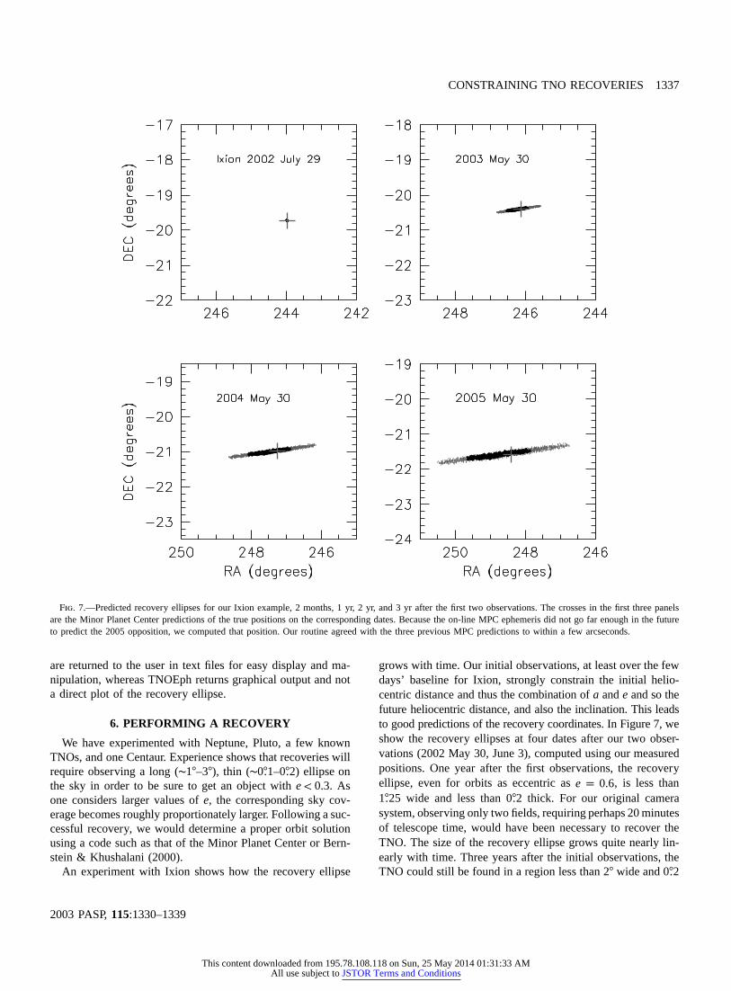
Fig. 7.—Predicted recovery ellipses for our Ixion example, 2 months, 1 yr, 2 yr, and 3 yr after the first two observations. The crosses in the first three panelsare the Minor Planet Center predictions of the true positions on the corresponding dates. Because the on-line MPC ephemeris did not go far enough in thefutureto predict the 2005 opposition, we computed that position. Our routine agreed with the three previous MPC predictions to within a few arcseconds.

are returned to the user in text files for easy display and ma-nipulation, whereas TNOEph returns graphical output and nota direct plot of the recovery ellipse.

6. PERFORMING A RECOVERY

We have experimented with Neptune, Pluto, a few knownTNOs, and one Centaur. Experience shows that recoveries willrequire observing a long (∼1�–3�), thin (∼0�.1–0�.2) ellipse onthe sky in order to be sure to get an object with . Ase ! 0.3one considers larger values ofe, the corresponding sky cov-erage becomes roughly proportionately larger. Following a suc-cessful recovery, we would determine a proper orbit solutionusing a code such as that of the Minor Planet Center or Bern-stein & Khushalani (2000).

An experiment with Ixion shows how the recovery ellipse

grows with time. Our initial observations, at least over the fewdays’ baseline for Ixion, strongly constrain the initial helio-centric distance and thus thecombination ofa ande and so thefuture heliocentric distance, and also the inclination. This leadsto good predictions of the recovery coordinates. In Figure 7, weshow the recovery ellipses at four dates after our two obser-vations (2002 May 30, June 3), computed using our measuredpositions. One year after the first observations, the recoveryellipse, even for orbits as eccentric as , is less thane p 0.61�.25 wide and less than 0�.2 thick. For our original camerasystem, observing only two fields, requiring perhaps 20 minutesof telescope time, would have been necessary to recover theTNO. The size of the recovery ellipse grows quite nearly lin-early with time. Three years after the initial observations, theTNO could still be found in a region less than 2� wide and 0�.2




2003 PASP,115:1330–1339

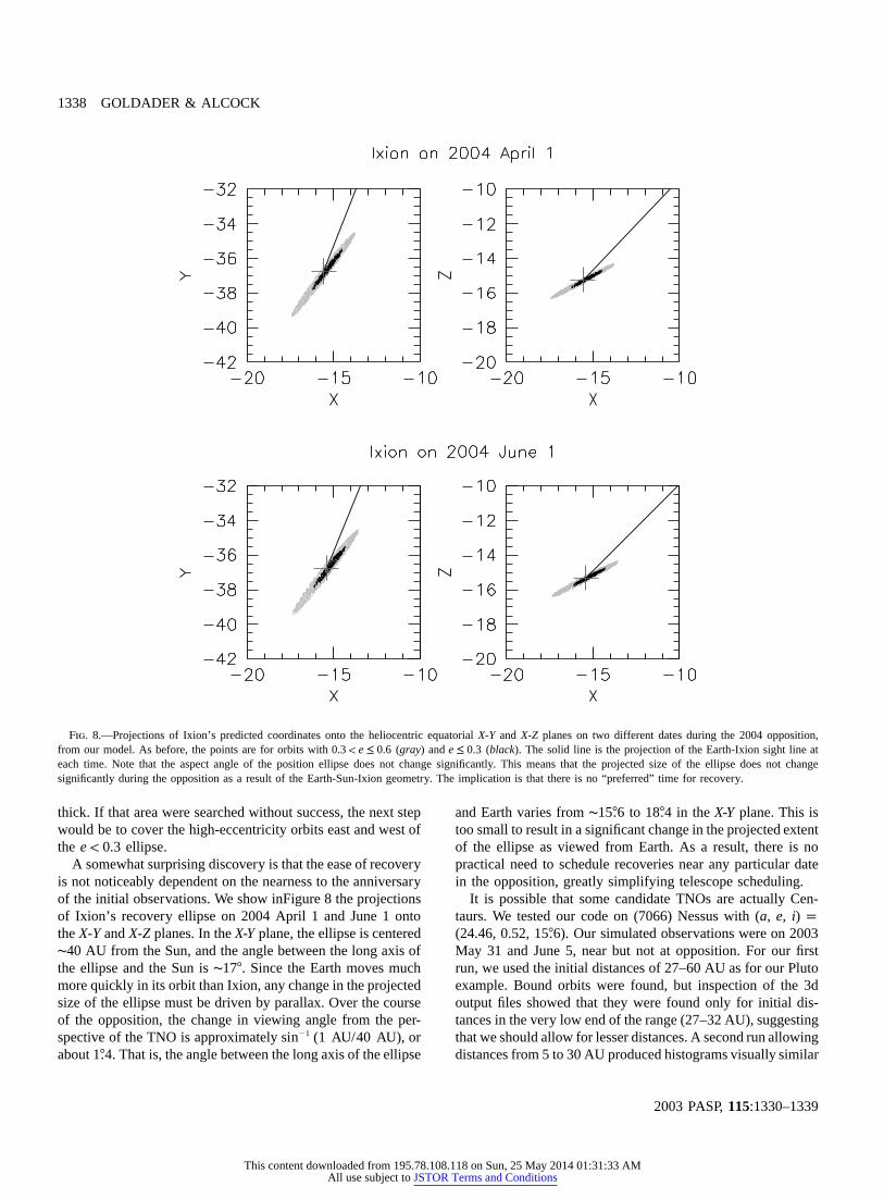
Fig. 8.—Projections of Ixion’s predicted coordinates onto the heliocentric equatorialX-Y and X-Z planes on two different dates during the 2004 opposition,from our model. As before, the points are for orbits with (gray) and (black). The solid line is the projection of the Earth-Ixion sight line at0.3! e ≤ 0.6 e ≤ 0.3each time. Note that the aspect angle of the position ellipse does not change significantly. This means that the projected size of the ellipse does not changesignificantly during the opposition as a result of the Earth-Sun-Ixion geometry. The implication is that there is no “preferred” time for recovery.

thick. If that area were searched without success, the next stepwould be to cover the high-eccentricity orbits east and west ofthe ellipse.e ! 0.3

A somewhat surprising discovery is that the ease of recoveryis not noticeably dependent on the nearness to the anniversaryof the initial observations. We show inFigure 8 the projectionsof Ixion’s recovery ellipse on 2004 April 1 and June 1 ontotheX-YandX-Z planes. In the plane, the ellipse is centeredX-Y∼40 AU from the Sun, and the angle between the long axis ofthe ellipse and the Sun is∼17�. Since the Earth moves muchmore quickly in its orbit than Ixion, any change in the projectedsize of the ellipse must be driven by parallax. Over the courseof the opposition, the change in viewing angle from the per-spective of the TNO is approximately , or�1sin (1 AU/40 AU)about 1�.4. That is, the angle between the long axis of the ellipse

and Earth varies from∼15�.6 to 18�.4 in the plane. This isX-Ytoo small to result in a significant change in the projected extentof the ellipse as viewed from Earth. As a result, there is nopractical need to schedule recoveries near any particular datein the opposition, greatly simplifying telescope scheduling.

It is possible that some candidate TNOs are actually Cen-taurs. We tested our code on (7066) Nessus with (a, e, i) p(24.46, 0.52, 15�.6). Our simulated observations were on 2003May 31 and June 5, near but not at opposition. For our firstrun, we used the initial distances of 27–60 AU as for our Plutoexample. Bound orbits were found, but inspection of the 3doutput files showed that they were found only for initial dis-tances in the very low end of the range (27–32 AU), suggestingthat we should allow for lesser distances. A second run allowingdistances from 5 to 30 AU produced histograms visually similar




2003 PASP,115:1330–1339

to those in Figure 2. The fitted values of the inclination werestrongly peaked at . For , the fitted values of16� � 2� e ≤ 0.6a ranged from approximately 12–28 AU. (High values ofemust be considered here, since Centaurs, being subject to stronggravitational perturbations from the outer planets, can havelarge orbital eccentricities.) Propagating the fitted orbits aheadto 2004 June 30, about a month before opposition, shows along recovery ellipse (6� in R.A., 3� in decl.) for , ande ! 0.6the actual position on that date is located within the ellipse,about half a degree west of the center. The long recovery ellipseis an unfortunate result of the need to consider large values ofthe eccentricity in this case. We suggest that in actual use ofour code, finding fitted orbits with initial distances packed nearone edge of the allowed range is a sign that the range shouldbe adjusted and the code run again.

Finally, we note that our code and recovery methodologyshould work well for other surveys of bright objects, but thatconfusion becomes an increasing problem at fainter magni-tudes. Consider our example of Ixion, searched for in 2004. Inour case, recovering the TNO would require scanning about0.3 deg2 within the recovery ellipse. The cumulativee ! 0.6luminosity function for (or CLF, the surface densityR ≤ 19.5of all objects brighter than , our expected limitingR p 19.5magnitude) is very low, estimated to be about deg�2�33 # 10(Trujillo, Jewitt, & Luu 2001). The chance of an interloper inour field is therefore very small, on the order of 10�3. The CLFrises with fainter magnitudes and reaches 3 deg�2 at R ≈ 24(Trujillo, Jewitt, & Luu 2001), which means we would expectone random interloper in our search field, and so isR ≈ 24

approximately the limit at which our method would work well.To have a surface density of 0.3 deg�2, so there is only a1/10 chance of an interloper in the search field, the TNO wouldhave to be brighter than . Should the initial recoveryR p 22.5images (at least two are needed to confirm motion) yield mul-tiple moving objects, the TNO being searched for might beidentifiable by trying to fit proper orbits to each candidate.

7. SUMMARY

We have presented a simple, easy-to-use, “brute-force”method that allows constraints to be placed on the area to besearched in order to recover a TNO observed just twice, overa time interval of just a few days. The results of our codecompare favorably to those of more rigorous programs. Thecode works for classical TNOs, as well as a typical Centaur.Observations can be made over a wide range of solar elon-gations, from the antisolar point to as far as∼50� from op-position. Results from our code compare favorably with thosefrom other programs, and our source code is publicly available.

It is our pleasure to thank Gary Bernstein for running com-parisons with his code, Jenni Virtanen for clearing up uncer-tainty in the proper use of TNOEph, and Rachel Moody, whoreviewed the manuscript prior to submission and provided help-ful suggestions. We thank the referee, James Bauer, for a timelyand helpful report. We gratefully acknowledge that this researchwas supported in part by the National Science Foundation,through grant AST 00-73845.

REFERENCES

Bernstein, G., & Khushalani, B. 2000, AJ, 120, 3323Duncan, M. J., Levison, H. F., & Budd, S. M. 1995, AJ, 110, 3073Gladman, B., et al. 2002, Icarus, 157, 269Holman, M. J., & Wisdom, J. 1993, AJ, 105, 1987Marsden, B. G. 1985, AJ, 90, 1541———. 1991, AJ, 102, 1539Marshall, S., et al. 2001, BAAS, 33, 3 (DPS Abstract 12.16)Millis, R. L., Buie, M. W., Wasserman, L. H., Elliot, J. L., Kern,

S. D., & Wagner, R. M. 2002, AJ, 123, 2083

Moody, R., et al. 2003, Proc. Int. Sci. Workshop on the First DecadalReview of the Edgeworth-Kuiper Belt: Towards New Frontiers, ed.J. Davies & L. Barrera (Dordrecht: Kluwer), in press

Sterne, T. E. 1960, An Introduction to Celestial Mechanics (New York:Interscience)

Trujillo, C. A., Jewitt, D. C., & Luu, J. X. 2001, AJ, 122, 457Virtanen, J., Muinonen, K., & Bowell, E. 2001, Icarus, 154, 412



Documents

Constraining Recovery Observations for Trans‐Neptunian Objects with Poorly Known Orbits