THE ASTROPHYSICAL JOURNAL LETTERS, MANUAL EMULATION TEMPLATE doi: 10.1088/2041-8205/XXX/X/LXX

1

CONSTRAINING SOLAR FLARE DIFFERENTIAL EMISSION MEASURES WITH EVE AND RHESSI

AMIR CASPI1, JAMES M. MCTIERNAN2, AND HARRY P. WARREN3

1Laboratory for Atmospheric and Space Physics, University of Colorado, Boulder, CO 80303, USA

2Space Sciences Laboratory University of California, Berkeley, CA 94720, USA 3Space Science Division, Naval Research Laboratory, Washington, DC 20375, USA

Received _____________; accepted _____________; published _____________

ABSTRACT Deriving a well-constrained differential emission measure (DEM) distribution for solar flares has historically been diffi-cult, primarily because no single instrument is sensitive to the full range of coronal temperatures observed in flares, from ≲2 to ≳50 MK. We present a new technique, combining extreme ultraviolet (EUV) spectra from the EUV Variability Experiment (EVE) onboard the Solar Dynamics Observatory with X-ray spectra from the Reuven Ramaty High Energy Solar Spectroscopic Imager (RHESSI), to derive, for the first time, a self-consistent, well-constrained DEM for jointly-observed solar flares. EVE is sensitive to ~2–25 MK thermal plasma emission, and RHESSI to ≳10 MK; together, the two instruments cover the full range of flare coronal plasma temperatures. We have validated the new technique on arti-ficial test data, and apply it to two X-class flares from solar cycle 24 to determine the flare DEM and its temporal evolu-tion; the constraints on the thermal emission derived from the EVE data also constrain the low-energy cutoff of the non-thermal electrons, a crucial parameter for flare energetics. The DEM analysis can also be used to predict the soft X-ray flux in the poorly-observed ~0.4–5 nm range, with important applications for geospace science. Key words: methods: data analysis — plasmas — radiation mechanisms: thermal — Sun: flares — Sun: UV radiation — Sun: X-rays, gamma rays

1. INTRODUCTION

Solar flares are powerful, explosive releases of magnetic energy, heating coronal plasma to tens of megaKelvin (MK) and accelerat-ing electrons to hundreds of MeV. The physical mechanisms be-hind these processes are still poorly understood (see the review by Fletcher et al. 2011). While it is commonly accepted that much of the hot coronal plasma results from energy deposition in the chro-mosphere by non-thermal, accelerated particles — “chromospher-ic evaporation” — X-ray observations, e.g., by Yohkoh or the Reu-ven Ramaty High Energy Solar Spectroscopic Imager (RHESSI; Lin et al. 2002), suggest significant in situ coronal heating, as well (e.g., Masuda 1994; Masuda et al. 1998; Caspi & Lin 2010; Long-cope & Guidoni 2011; Caspi et al. 2014), although the specific mechanism is still debated. Another crucial problem lies in identi-fying the low-energy cutoff/rollover of the accelerated electron spectrum, required by energetics (see the review by Holman et al. 2011) but typically poorly constrained as its observable manifesta-tion — a rollover of the non-thermal bremsstrahlung spectrum (cf. Brown 1971) — is often obscured by thermal bremsstrahlung emission that dominates the photon spectrum up to ~20–35 keV in intense flares.

These questions remain, in large part, because of the difficulty in accurately and precisely characterizing the thermal electron population in flares. While flare analyses often employ the iso-thermal approximation (e.g., Lin et al. 1981; Garcia 1994; Feld-man et al. 1996; Holman et al. 2003), decades of extreme ultravio-let (EUV) and X-ray observations with widely varying tempera-ture sensitivities have shown that flare plasma exhibits a distribu-tion of emission measure with temperature (the “differential emis-sion measure,” or DEM). Nonetheless, there have been only a few previous studies of solar flare DEMs (e.g., Dere & Cook 1979; McTiernan et al. 1999; Chifor et al. 2007; see also Trottet et al. 2011, who derived a four-component discretized model for one flare); stellar DEMs have been analyzed more extensively (see, e.g., the reviews by Bowyer et al. 2000; Favata & Micela 2003; Güdel & Nazé 2009; and references therein).

Deriving a well-constrained flare DEM has proven difficult, largely because no single instrument’s temperature response en-

compasses the full dynamic range of observed coronal tempera-tures. EUV instruments are not sensitive above ~25 MK, where the EUV-emitting ion species become depleted, and historically have suffered from poor spectral resolution (e.g., broadband fil-ters) or coverage (e.g., narrowband filters), and/or poor temporal resolution (e.g., due to slit rastering). X-ray instruments typically become sensitivity-limited below ~10 MK, and temperatures in-ferred from spectral lines of hydrogen- and helium-like heavy ions (e.g., Fe, Ca, Si, etc.) often disagree significantly with those in-ferred from continuum emission (e.g., Phillips et al. 2006; Caspi & Lin 2010). A self-consistent solution has yet to be found (cf. Ryan et al. 2014).

The EUV Variability Experiment (EVE; Woods et al. 2012) onboard the Solar Dynamics Observatory (SDO; Pesnell et al. 2012) finally provides the means of addressing this issue compre-hensively. EVE’s broadband coverage, including sensitivity to all EUV-emitting ion temperatures of ~1–25 MK, combined with RHESSI’s sensitivity to all temperatures ≳10 MK, provides com-plete coverage of the full range of coronal plasma temperatures observed in flares with sufficient cadence to study their temporal evolution. We present a new diagnostic technique to derive a self-consistent, well-constrained DEM for jointly-observed flares, by simultaneously analyzing EVE and RHESSI full-Sun spectra. We apply this technique to derive the time-series DEMs for the impul-sive and decay phases of two X-class flares and present the first results of the inferred thermal parameters. DEMs derived through this technique can also be used to generate synthetic soft X-ray (SXR) and EUV spectra, with important applications for the geo-space community.

2. METHOD DETAILS

The EVE suite comprises multiple instruments, including broadband photometers and high-resolution spectrometers that to-gether measure solar EUV/SXR emission from ~0.1 to ~105 nm (Woods et al. 2012). We focus on the Multiple EUV Grating Spectrograph A (MEGS-A), a grazing-incidence dual-slit spectro-graph measuring the spatially integrated solar spectral irradiance from ~5 to ~37 nm, with ~0.1 nm FWHM resolution and 10 s ca-

THE ASTROPHYSICAL JOURNAL LETTERS, XXX:LXX (Xpp), 20XX Month X CASPI, MCTIERNAN, & WARREN

2

dence (Hock et al. 2012). The MEGS-A wavelength range in-cludes numerous spectral lines from various ion species with for-mation temperatures from ~1 to ~25 MK. The 9–15 nm range is particularly rich in high-temperature lines, including most of the strongest Fe XVIII–XXIII lines (peak formation temperatures of ~6–15 MK; cf. Mazzotta et al. 1998); MEGS-A also observes Fe XXIV (~20 MK) at 19.204 and 25.510 nm, and Fe XV (~2 MK) and XVI (~3 MK) at 28.416 and 33.541 nm, respectively, among many other lines. This wealth of temperature diagnostics enables the most precise determination of the flare DEM to date (Warren et al. 2013), especially from EUV observations, although they remain poorly constrained for temperatures ≳25 MK, where EVE has lit-tle or no temperature sensitivity (Figure 1). This can be somewhat mitigated by adding observations from the X-ray Sensor (XRS) on the Geostationary Operational Environmental Satellite (GOES), but the two-channel broadband XRS measurements — from which temperatures can also be inferred (e.g., White et al. 2005) — add minimal spectral information and extend the DEM validity only up to ~30 MK (Warren et al. 2013).

Significantly stronger constraints can be obtained using RHESSI (Lin et al. 2002), which measures solar hard X-rays (HXRs) be-low ~0.4 nm with ≲0.1 nm FWHM resolution (quasi-constant ~1 keV when expressed in photon energy, variable ~λ2/hc expressed in wavelength; Smith et al. 2002). RHESSI provides the most pre-cise measurements of thermal X-ray continuum emission from plasmas with temperatures ≳10 MK, and is especially sensitive to the hottest part of the temperature distribution, up to ≳50 MK (e.g., Caspi et al. 2014). While RHESSI data can be used for DEM studies in isolation, RHESSI’s “temperature resolution” is broad because of the inherent “smoothing” of the bremsstrahlung emis-sion mechanism; it is therefore difficult to recover a high-temperature-resolution DEM even from the high-temporal- and -spectral-resolution continuum photon spectra, and the data often cannot sufficiently distinguish between a dual-isothermal model (delta-function DEM) or a continuous DEM (e.g., Caspi & Lin 2010; McTiernan & Caspi 2014). The inferred DEM is also not well-constrained below ~10–15 MK, where the HXR yield is low and observations are typically limited by sensitivity or dynamic range (emission from the hotter parts of the DEM dominate the RHESSI spectra). EUV observations are required to provide these constraints.

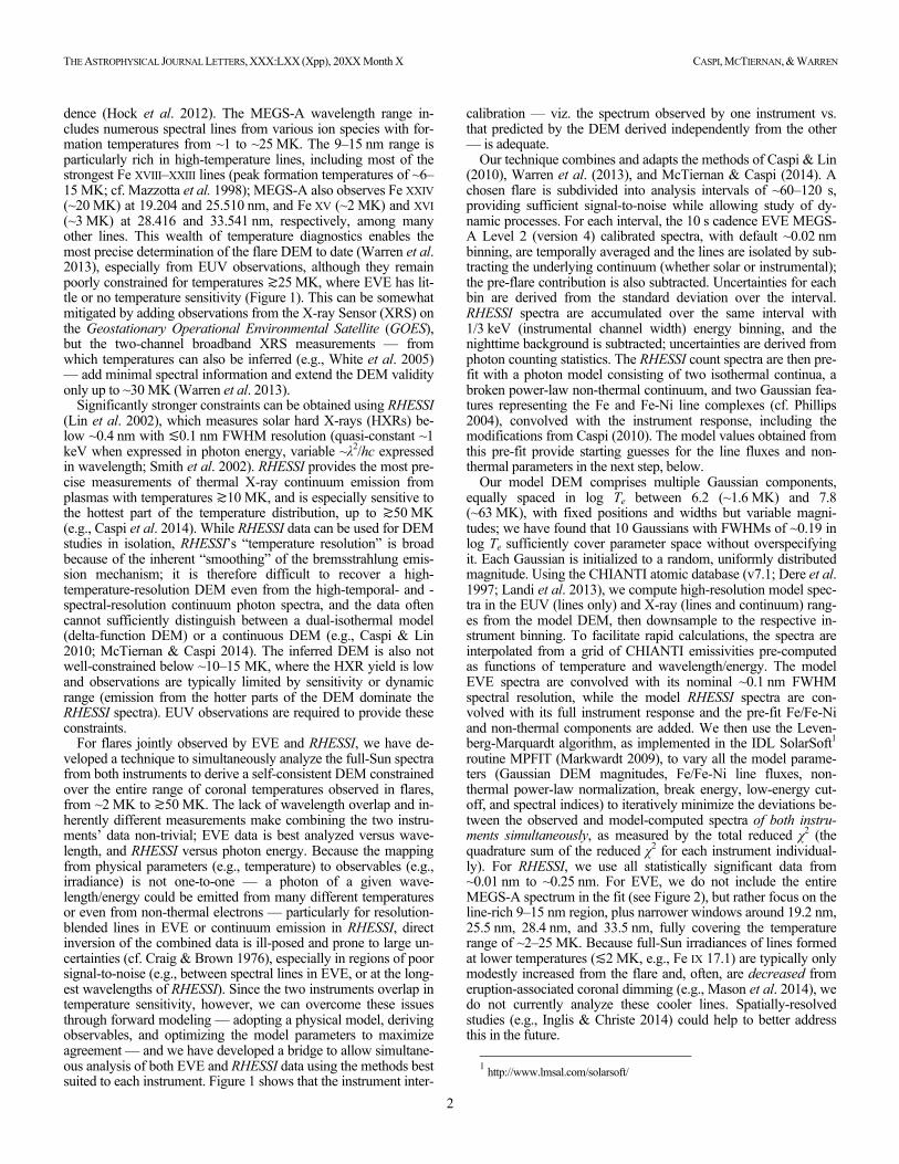
For flares jointly observed by EVE and RHESSI, we have de-veloped a technique to simultaneously analyze the full-Sun spectra from both instruments to derive a self-consistent DEM constrained over the entire range of coronal temperatures observed in flares, from ~2 MK to ≳50 MK. The lack of wavelength overlap and in-herently different measurements make combining the two instru-ments’ data non-trivial; EVE data is best analyzed versus wave-length, and RHESSI versus photon energy. Because the mapping from physical parameters (e.g., temperature) to observables (e.g., irradiance) is not one-to-one — a photon of a given wave-length/energy could be emitted from many different temperatures or even from non-thermal electrons — particularly for resolution-blended lines in EVE or continuum emission in RHESSI, direct inversion of the combined data is ill-posed and prone to large un-certainties (cf. Craig & Brown 1976), especially in regions of poor signal-to-noise (e.g., between spectral lines in EVE, or at the long-est wavelengths of RHESSI). Since the two instruments overlap in temperature sensitivity, however, we can overcome these issues through forward modeling — adopting a physical model, deriving observables, and optimizing the model parameters to maximize agreement — and we have developed a bridge to allow simultane-ous analysis of both EVE and RHESSI data using the methods best suited to each instrument. Figure 1 shows that the instrument inter-

calibration — viz. the spectrum observed by one instrument vs. that predicted by the DEM derived independently from the other — is adequate.

Our technique combines and adapts the methods of Caspi & Lin (2010), Warren et al. (2013), and McTiernan & Caspi (2014). A chosen flare is subdivided into analysis intervals of ~60–120 s, providing sufficient signal-to-noise while allowing study of dy-namic processes. For each interval, the 10 s cadence EVE MEGS-A Level 2 (version 4) calibrated spectra, with default ~0.02 nm binning, are temporally averaged and the lines are isolated by sub-tracting the underlying continuum (whether solar or instrumental); the pre-flare contribution is also subtracted. Uncertainties for each bin are derived from the standard deviation over the interval. RHESSI spectra are accumulated over the same interval with 1/3 keV (instrumental channel width) energy binning, and the nighttime background is subtracted; uncertainties are derived from photon counting statistics. The RHESSI count spectra are then pre-fit with a photon model consisting of two isothermal continua, a broken power-law non-thermal continuum, and two Gaussian fea-tures representing the Fe and Fe-Ni line complexes (cf. Phillips 2004), convolved with the instrument response, including the modifications from Caspi (2010). The model values obtained from this pre-fit provide starting guesses for the line fluxes and non-thermal parameters in the next step, below.

Our model DEM comprises multiple Gaussian components, equally spaced in log Te between 6.2 (~1.6 MK) and 7.8 (~63 MK), with fixed positions and widths but variable magni-tudes; we have found that 10 Gaussians with FWHMs of ~0.19 in log Te sufficiently cover parameter space without overspecifying it. Each Gaussian is initialized to a random, uniformly distributed magnitude. Using the CHIANTI atomic database (v7.1; Dere et al. 1997; Landi et al. 2013), we compute high-resolution model spec-tra in the EUV (lines only) and X-ray (lines and continuum) rang-es from the model DEM, then downsample to the respective in-strument binning. To facilitate rapid calculations, the spectra are interpolated from a grid of CHIANTI emissivities pre-computed as functions of temperature and wavelength/energy. The model EVE spectra are convolved with its nominal ~0.1 nm FWHM spectral resolution, while the model RHESSI spectra are con-volved with its full instrument response and the pre-fit Fe/Fe-Ni and non-thermal components are added. We then use the Leven-berg-Marquardt algorithm, as implemented in the IDL SolarSoft1 routine MPFIT (Markwardt 2009), to vary all the model parame-ters (Gaussian DEM magnitudes, Fe/Fe-Ni line fluxes, non-thermal power-law normalization, break energy, low-energy cut-off, and spectral indices) to iteratively minimize the deviations be-tween the observed and model-computed spectra of both instru-ments simultaneously, as measured by the total reduced χ2 (the quadrature sum of the reduced χ2 for each instrument individual-ly). For RHESSI, we use all statistically significant data from ~0.01 nm to ~0.25 nm. For EVE, we do not include the entire MEGS-A spectrum in the fit (see Figure 2), but rather focus on the line-rich 9–15 nm region, plus narrower windows around 19.2 nm, 25.5 nm, 28.4 nm, and 33.5 nm, fully covering the temperature range of ~2–25 MK. Because full-Sun irradiances of lines formed at lower temperatures (≲2 MK, e.g., Fe IX 17.1) are typically only modestly increased from the flare and, often, are decreased from eruption-associated coronal dimming (e.g., Mason et al. 2014), we do not currently analyze these cooler lines. Spatially-resolved studies (e.g., Inglis & Christe 2014) could help to better address this in the future.

1 http://www.lmsal.com/solarsoft/

THE ASTROPHYSICAL JOURNAL LETTERS, XXX:LXX (Xpp), 20XX Month X CASPI, MCTIERNAN, & WARREN

3

Because forward modeling does not guarantee uniqueness — different DEMs could potentially yield the same observed spectra, within uncertainties — we fit each interval 100 times in a Monte Carlo process. By using different model initial conditions — a new random DEM, and perturbed Fe/Fe-Ni line fluxes and non-thermal parameters — and by perturbing the observed spectra by their uncertainties for each trial, we effectively sample parameter space to test for multiple solutions (local χ2 minima) and derive uncertainties for each one; 100 trials provides a sufficient con-straint on stability.

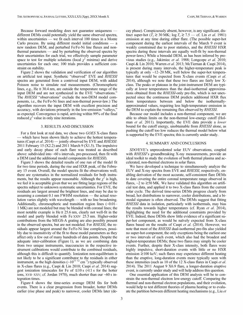
Figure 2 shows the validation and verification of our algorithm on artificial test input. Synthetic “observed” EVE and RHESSI spectra are generated from a contrived input DEM, with added Poisson noise to simulate real measurements. (Chromospheric lines, e.g., He II 30.4 nm, are outside the temperature range of the input DEM and are not synthesized in the EVE “observations.” The RHESSI “observations” exclude the non-DEM model com-ponents, i.e., the Fe/Fe-Ni lines and non-thermal power-law.) The algorithm recovers the input DEM with excellent precision and accuracy, with deviations primarily in the low-emission “valleys,” as expected. Convergence is rapid, arriving within 99% of the final reduced χ2 value in only nine iterations.

3. RESULTS AND DISCUSSION

For a first look at real data, we chose two GOES X-class flares — which have been shown likely to achieve the hottest tempera-tures (Caspi et al. 2014) — jointly observed by EVE and RHESSI: 2011 February 15 (X2.2) and 2011 March 9 (X1.5). The impulsive and early decay phase of each flare was treated as described above: subdivided into ~60 s intervals, pre-processed, then fit with a DEM (and the additional model components for RHESSI).

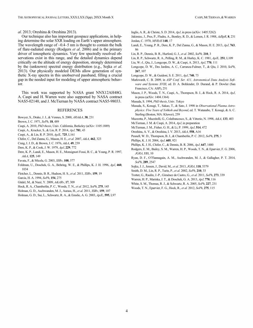
Figure 3 shows the detailed results of one run of the model fit for two time periods, during the rise and HXR peak, of the Febru-ary 15 event. Overall, the model spectra fit the observations well; there are systematics in the normalized residuals for both instru-ments, but the results appear reasonable. Although the χ2 is high, we feel it is acceptable given that we are fitting large regions of the spectra subject to unknown systematic uncertainties. For EVE, the residuals are largest around the brightest lines, and may be due to assuming a constant 0.1 nm FWHM resolution — the actual reso-lution varies slightly with wavelength — with no line broadening. Additionally, chromospheric and transition region lines (~0.01–1 MK) are not modeled but may be blended with coronal lines; the most notable example is He II 25.6 nm, clearly not well-fit in the model and partly blended with Fe XXIV 25.5 nm. Higher-order contributions from the MEGS-A grating are also possibly present in the observed spectra, but are not modeled. For RHESSI, the re-siduals appear largest around the Fe/Fe-Ni line complexes, possi-bly due to insensitivity of the fit to these model parameters as they affect only a few out of many hundreds of data points. Despite the adequate inter-calibration (Figure 1), as we are combining data from two unique instruments, inaccuracies in the respective in-strument calibrations would contribute to the combined residuals, although this is difficult to quantify. Ionization non-equilibrium is not likely to be a significant contributor to the residuals in either instrument, as the high densities (~1011–12 cm–3) typically observed in X-class flares (e.g., Caspi & Lin 2010; Caspi et al. 2014) sug-gest ionization timescales for Fe of ≲10 s (≪1 s for the hotter ions, XVII–XXV; cf. Jordan 1970), much shorter than our ~60 s in-tegration times.

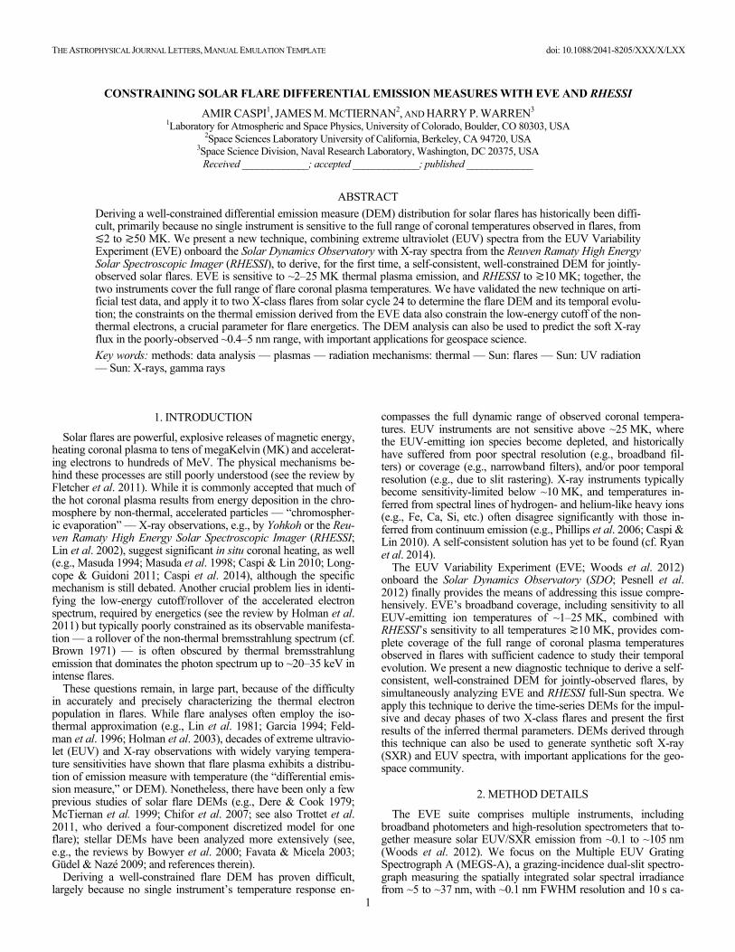
Figure 4 shows the time-series average DEM fits for both events. There is a clear progression from broader, hotter DEMs earlier (rise phase and peak) to narrower, cooler DEMs later (de-

cay phase). Conspicuously absent, however, is any significant, dis-tinct super-hot (Te ≳ 30 MK; log Te ≳ 7.5 — cf. Lin et al. 1981) emission at any time during either flare. (The possible super-hot component during the earliest intervals of the March 9 event is weakly constrained due to poor statistics, and the RHESSI HXR spectra during these intervals are equally well-fit by non-thermal power-laws.) While a bimodal DEM, as has been inferred by pre-vious studies (e.g., Jakimiec et al. 1988; Longcope et al. 2010; Caspi & Lin 2010; Warren et al. 2013; McTiernan & Caspi 2014), is present during many intervals, the higher-temperature peak is typically at only ~12–20 MK, well below the super-hot tempera-tures that would be expected from X-class events (Caspi et al. 2014), although we note that these two flares are fairly low X-class. The peaks or plateaus in the joint-instrument DEM are typi-cally at lower temperatures than the dual-isothermal approxima-tions obtained from the RHESSI-only pre-fits, which is not unex-pected since the continuous DEM predicts additional HXR flux from temperatures between and below the isothermally-approximated values, requiring less high-temperature emission in the DEM to explain the remaining flux observed by RHESSI.

Because our model includes a non-thermal component, we are able to obtain limits on the non-thermal low-energy cutoff (Hol-man et al. 2011). Importantly, the EVE data provide a lower bound for the cutoff energy, unobtainable from RHESSI alone, as pushing the cutoff too low reduces the thermal model below what is supported by the EVE spectra; this is currently under study.

4. SUMMARY AND CONCLUSIONS

SDO/EVE’s unprecedented solar EUV observations, coupled with RHESSI’s groundbreaking X-ray measurements, provide an ideal toolkit to study the evolution of both thermal plasma and ac-celerated, non-thermal electrons in solar flares.

We have developed a technique to simultaneously analyze the EUV and X-ray spectra from EVE and RHESSI, respectively, en-abling derivation of the most accurate, self-consistent flare DEMs to date covering the entire coronal temperature range observed in flares, ~2 to ≳50 MK. We have validated this algorithm on artifi-cial test data, and applied it to two X-class flares from the current solar cycle. The derived time-series DEMs progress clearly from broad, hot distributions to narrower, cooler distributions, and a bi-modal signature is often observed. The DEMs suggest that fitting RHESSI data in isolation, particularly with isothermals, may bias the results towards higher temperatures (cf. Ryan et al. 2014), highlighting the need for the additional constraints provided by EVE. Indeed, these DEMs show little evidence of a significant su-per-hot component, as would be naïvely expected from X-class flares based on the results of Caspi et al. (2014). However, we note that most of the RHESSI dual-isothermal pre-fits also yielded no super-hot component, the only exceptions being the earliest one or two intervals of each event, which also had the broadest and highest-temperature DEMs; these two flares may simply be cooler events. Further, despite their X-class intensity, both flares were highly impulsive, short-duration events with little or no HXR emission ≳100 keV; such flares may experience different heating than the eruptive, long-duration events more typically seen with these intensities (such as 10 of the 12 X-class flares in Caspi et al. 2014). The 2011 August 9 X6.9 flare, a longer-duration eruptive event, is currently under study and will help address this question.

One essential application of this DEM analysis will be to con-strain the non-thermal electron low-energy cutoff. Comparing the thermal and non-thermal electron populations, and their evolution, would help to test different theories of plasma heating or to evalu-ate the partition between different heating mechanisms (e.g., Liu et

THE ASTROPHYSICAL JOURNAL LETTERS, XXX:LXX (Xpp), 20XX Month X CASPI, MCTIERNAN, & WARREN

4

al. 2013; Oreshina & Oreshina 2013). Our technique also has important geospace applications, in help-

ing determine the solar SXR loading on Earth’s upper atmosphere. The wavelength range of ~0.4–5 nm is thought to contain the bulk of flare-radiated energy (Rodgers et al. 2006) and is the primary driver of ionospheric dynamics. Very few spectrally resolved ob-servations exist in this range, and the detailed dynamics depend critically on the altitude of energy deposition, strongly determined by the (unknown) spectral energy distribution (e.g., Sojka et al. 2013). Our physically modeled DEMs allow generation of syn-thetic X-ray spectra in this unobserved passband, filling a crucial gap in the needed input for modeling of upper atmospheric behav-ior.

This work was supported by NASA grant NNX12AH48G.

A. Caspi and H. Warren were also supported by NASA contract NAS5-02140, and J. McTiernan by NASA contract NAS5-98033.

REFERENCES

Bowyer, S., Drake, J. J., & Vennes, S. 2000, ARA&A, 38, 231 Brown, J. C. 1971, SoPh, 18, 489 Caspi, A. 2010, PhD thesis, Univ. California, Berkeley (arXiv: 1105.1889) Caspi, A., Krucker, S., & Lin, R. P. 2014, ApJ, 781, 43 Caspi, A., & Lin, R. P. 2010, ApJL, 725, L161 Chifor, C., Del Zanna, G., Mason, H. E., et al. 2007, A&A, 462, 323 Craig, I. J. D., & Brown, J. C. 1976, A&A, 49, 239 Dere, K. P., & Cook, J. W. 1979, ApJ, 229, 772 Dere, K. P., Landi, E., Mason, H. E., Monsignori Fossi, B. C., & Young, P. R. 1997,

A&A, 125, 149 Favata, F., & Micela, G. 2003, SSRv, 108, 577 Feldman, U., Doschek, G. A., Behring, W. E., & Phillips, K. J. H. 1996, ApJ, 460,

1034 Fletcher, L., Dennis, B. R., Hudson, H. S., et al. 2011, SSRv, 159, 19 Garcia, H. A. 1994, SoPh, 154, 275 Güdel, M., & Nazé, Y. 2009, A&ARv, 17, 309 Hock, R. A., Chamberlin, P. C., Woods, T. N., et al. 2012, SoPh, 275, 145 Holman, G. D., Aschwanden, M. J., Aurass, H., et al. 2011, SSRv, 159, 107 Holman, G. D., Sui, L., Schwartz, R. A., & Emslie, A. G. 2003, ApJL, 595, L97

Inglis, A. R., & Christe, S. D. 2014, ApJ, in press (arXiv: 1405.5262) Jakimiec, J., Pres, P., Fludra, A., Bentley, R. D., & Lemen, J. R. 1988, AdSpR, 8, 231 Jordan, C. 1970, MNRAS 148, 17 Landi, E., Young, P. R., Dere, K. P., Del Zanna, G., & Mason, H. E. 2013, ApJ, 763,

86 Lin, R. P., Dennis, B. R., Hurford, G. J., et al. 2002, SoPh, 210, 3 Lin, R. P., Schwartz, R. A., Pelling, R. M., & Hurley, K. C. 1981, ApJL, 251, L109 Liu, W.-J., Qiu, J., Longcope, D. W., & Caspi, A. 2013, ApJ, 770, 111 Longcope, D. W., Des Jardins, A. C., Carranza-Fulmer, T., & Qiu, J. 2010, SoPh,

267, 107 Longcope, D. W., & Guidoni, S. E. 2011, ApJ, 740, 73 Markwardt, C. B. 2009, in ASP Conf. Ser. 411, Astronomical Data Analysis Soft-

ware and Systems XVIII, ed. D. A. Bohlender, D. Durand, & P. Dowler (San Francisco, CA: ASP), 251

Mason, J. P., Woods, T. N., Caspi, A., Thompson, B. J., & Hock, R. A. 2014, ApJ, in press (arXiv: 1404.1364)

Masuda, S. 1994, PhD thesis, Univ. Tokyo Masuda, S., Kosugi, T., Sakao, T., & Sato, J. 1998 in Observational Plasma Astro-

physics: Five Years of Yohkoh and Beyond, ed. T. Watanabe, T. Kosugi, & A. C. Sterling (Boston, MA: Kluwer), 259

Mazzotta, P., Mazzitelli, G., Colafrancesco, S., & Vittorio, N. 1998, A&A, 133, 403 McTiernan, J. M. & Caspi, A. 2014, ApJ, in preparation McTiernan, J. M., Fisher, G. H., & Li, P. 1999, ApJ, 514, 472 Oreshina, A. V., & Oreshina, I. V. 2013, A&A, 558, A16 Pesnell, W. D., Thompson, B. J., & Chamberlin, P. C. 2012, SoPh, 275, 3 Phillips, K. J. H. 2004, ApJ, 605, 921 Phillips, K. J. H., Chifor, C., & Dennis, B. R. 2006, ApJ, 647, 1480 Rodgers, E. M., Bailey, S. M., Warren, H. P., Woods, T. N., & Eparvier, F. G. 2006,

JGRA, 111, 10 Ryan, D. F., O’Flannagain, A. M., Aschwanden, M. J., & Gallagher, P. T. 2014,

SoPh, 289, 2547 Sojka, J. J., Jensen, J., David, M., et al. 2013, JGRA, 118, 5379 Smith, D. M., Lin, R. P., Turin, P., et al. 2002, SoPh, 210, 33 Trottet, G., Raulin, J.-P., Giménez de Castro, G., et al. 2011, SoPh, 273, 339 Warren, H. P., Mariska, J. T., & Doschek, G. A. 2013, ApJ, 770, 116 White, S. M., Thomas, R. J., & Schwartz, R. A. 2005, SoPh, 227, 231 Woods, T. N., Eparvier, F. G., Hock, R., et al. 2012, SoPh, 275, 115

DEM Comparison – 2011 Mar 09, 23:21 UT

1 10 100T (MK)

10−10

10−8

10−6

10−4

10−2

100

102

104

EM (1

049 cm

–3)

+

Black: RHESSI DEMGreen: RHESSI 2TBlue: GOES IsoTRed: EVE DEM

Count Rate Comparison – 2011 Mar 09, 23:21 UT

10 30 503 5 10 30 503 5Energy (keV)

10−3

10−2

10−1

100

101

102

103

104

Coun

t Rat

eBlack: RHESSIRed: from EVE DEMBlue: from GOES IsoT

Energy (keV)

Black: RHESSIRed: from EVE DEM <30 MKBlue: from GOES IsoT

Figure 1. [left] DEMs derived from RHESSI (black) and EVE (red) data in isolation, with RHESSI dual-isothermal pre-fit (green plusses) and GOES XRS isothermal (blue plus) for comparison. The RHESSI DEM has limited resolution and poor constraints ≲10 MK; the EVE DEM is better resolved but poorly constrained ≳25 MK. [center] Observed RHESSI count rate spectrum vs. photon energy (black) and synthetic models derived from the EVE DEM (red) and GOES isothermal (blue); the high-temperature excess in the EVE-derived model overestimates observations by ≳10×. The GOES-derived model agrees well at low energies, but indicates need for a higher-temperature component, consistent with the dual-isothermal fit. [right] Arbitrarily truncating the EVE DEM at ~30 MK yield good model agreement with RHESSI at lower energies, consistent with the GOES-derived model, and suggests that the instrument inter-calibration is adequate.

30 503 5

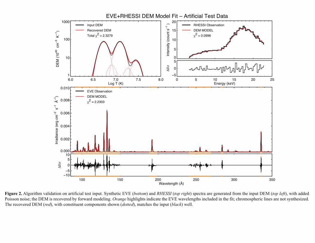
Figure 2. Algorithm validation on artificial test input. Synthetic EVE (bottom) and RHESSI (top right) spectra are generated from the input DEM (top left), with added Poisson noise; the DEM is recovered by forward modeling. Orange highlights indicate the EVE wavelengths included in the fit; chromospheric lines are not synthesized. The recovered DEM (red), with constituent components shown (dotted), matches the input (black) well.

0.000

0.002

0.004

0.006

0.008

0.010

Irrad

iance

(erg

cm−2

s−1 Å

−1)

EVE ObservationDEM MODELχ2 = 2.2303

100 150 200 250 300 350Wavelength (Å)

−10−5

05

10

ΔI/σ

6.0 6.5 7.0 7.5 8.0Log T (K)

1

10

100

1000

DEM

(1040

cm−3

K−1

)

Input DEMRecovered DEMTotal χ2 = 2.3279

0

5

10

15

20

Inte

nsity

(cou

nt s−1

) RHESSI ObservationDEM MODELχ2 = 0.0996

0 5 10 15 20 25Energy (keV)

−505

ΔI/σ

EVE+RHESSI DEM Model Fit – Artificial Test Data

Figure 3. DEM fits from two intervals of the 2011 February 15 X2.2 event, during the rise (~01:51 UTC; left) and HXR peak (~01:53 UTC; right). Systematics exist in the normalized residuals for both instruments, but the fits are reasonable, with acceptable χ2 considering that entire spectral regions are being fit and accounting for model-ing limitations.

0.000

0.005

0.010

0.015

0.020

0.025

0.030

Irrad

iance

(erg

cm−2

s−1 Å

−1)

EVE ObservationDEM MODELχ2 = 13.32

100 150 200 250 300 350Wavelength (Å)

−40−20

02040

ΔI/σ

6.0 6.5 7.0 7.5 8.0Log T (K)

1

10

100

1000

DEM

(1040

cm−3

K−1

)

Recovered DEMTotal χ2 = 16.23

0

50

100

150

200250

Inte

nsity

(cou

nt s−1

) RHESSI ObsDEM MODELχ2 = 2.91A0: 4.37 γ1: 1.50Ebr1: 8.45 γ2: 3.96Fe: 6.05 FeNi: 5.19

0 20 40 60 80Energy (keV)

−100

10

ΔI/σ

0.000

0.002

0.004

0.006

0.008

0.010

Irrad

iance

(erg

cm−2

s−1 Å

−1)

EVE ObservationDEM MODELχ2 = 5.95

100 150 200 250 300 350Wavelength (Å)

−20−10

01020

ΔI/σ

6.0 6.5 7.0 7.5 8.0Log T (K)

1

10

100

1000

DEM

(1040

cm−3

K−1

)

Recovered DEMTotal χ2 = 6.81

0

20406080

100120

Inte

nsity

(cou

nt s−1

) RHESSI ObsDEM MODELχ2 = 0.85A0: 6.25 γ1: 1.50Ebr1: 6.53 γ2: 6.02Fe: 5.55 FeNi: 4.51

0 20 40 60 80Energy (keV)

−505

ΔI/σ

2011 Feb 15 – 01:51 UTC 2011 Feb 15 – 01:53 UTC

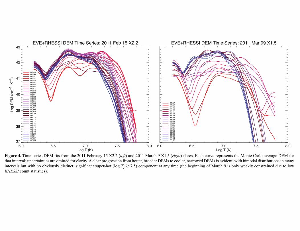
Figure 4. Time-series DEM fits from the 2011 February 15 X2.2 (left) and 2011 March 9 X1.5 (right) flares. Each curve represents the Monte Carlo average DEM for that interval; uncertainties are omitted for clarity. A clear progression from hotter, broader DEMs to cooler, narrowed DEMs is evident, with bimodal distributions in many intervals but with no obviously distinct, significant super-hot (log Te ≳ 7.5) component at any time (the beginning of March 9 is only weakly constrained due to low RHESSI count statistics).

EVE+RHESSI DEM Time Series: 2011 Feb 15 X2.2

6.0 6.5 7.0 7.5 8.0Log T (K)

37

38

39

40

41

42

43

Log

DEM

(cm

−3 K

−1)

01:4901:5001:5101:5201:5301:5401:5501:5601:5701:5802:0002:0102:0202:0302:0402:0502:0602:0702:0802:0902:1002:1102:1202:1302:1402:1502:1602:1702:1802:1902:2002:2102:2202:23

EVE+RHESSI DEM Time Series: 2011 Mar 09 X1.5

6.0 6.5 7.0 7.5 8.0Log T (K)

23:1723:1823:1923:1923:2023:2123:2223:2423:2523:2623:2723:2823:2923:3023:3123:3223:3323:3423:35