Contagion and ranking processes in complex networks: the role of geography and interactionstrength

PhD Thesis Proposal

Qian ZhangCollege of Computer and Information Science

Northeastern University, Boston, MA

January 14, 2014

Abstract

The recent global surge in the use of technologies such as social media, smart phones and GPS-enabled devices hasprovided abundant resources to understand dynamical processes on complex networks and a unique chance to characterizegeospatial and temporal distribution of real time social events. Meanwhile, the easy accessibility to bibliographic dataand geographical database allow better understanding of scholarly networks and in charting the creation of knowledgeglobally. Moreover, the availability of large-scale communication datasets presents new opportunities to study informationdissemination on social networks. In this thesis we focus on the diffusion processes on complex networks aggregatedfrom these data. First, we investigate geospatial and temporal features of a publication dataset. We characterize theknowledge diffusion pattern between worldwide urban areas and its temporal evolution, and identify the key cities in thescientific research in physics. Second, we propose to detect and predict seasonal flu epidemics in countries of interest withgeolocalized Twitter signals. In the early stage of a flu season, tweets containing information related with influenza-likeillness indicate the spatial distribution of possible initial infected cases. Modeling disease and spreading dynamics withthese initial seeds can provide the possibility of forecasting ILI cases in the coming month. Beyond geospatial information,we also investigate the role of other network properties play on information diffusion process. For a human-to-humancommunication network, we survey different definitions of weak ties and develop a novel link property importance tocharacterize the strength of ties. Controlling weak ties defined by importance can more efficiently confine the informationspreading within a small community than controlling weak ties under other definitions. Last but not least, we find a phasetransition between absorbing and active states of the classic Maki-Thompson rumor spreading model on random networks.The parameters of the contagion process as well as the network architecture determine whether the rumor will spreadglobally or whether it will be confined within a small neighborhood.

1 Introduction

Digital records of social interactions and publication datasets have been increasingly accessible in the past decade. Thesehigh resolution and large-scale datasets obtained through Internet, mobile devices and pervasive technologies have en-abled a wealth of research in dynamical processes occurring on top of complex networks [71, 11]. Digitalization of bib-liographic data help understanding the geospatial distribution of millions of publications, and citations at different gran-ularities [12, 51, 42, 33, 64, 56]. Considering the geographical spread of human infectious diseases, data-driven com-putational models [9] have been proven to be indispensable tools in guiding public health policies by the availability ofhuman mobility datasets at large scale [25, 7]. Moreover, these data have enabled the theoretical understanding of criti-cal phenomena of nonequilibrium phase transitions in infectious disease spread mediated by complex network structuresand mobility schemes [26, 10]. Similarly, accessibility of highly detailed mobile phone communication datasets at largescale [62, 50, 48, 18, 49] provides unique opportunities for studying information diffusion in real social systems from boththeoretical and computational points of view. Furthermore, online social network platforms such as Twitter provide abun-dant sources of real time events. Each user on such the platform can be considered as a social sensor and each tweet assensory information [67]. These social sensors provide a unique chance to detect and predict real time social events such asearthquake [67] flu [27, 3], election [70], reality-singing competition [24]. In this thesis work, we take advantage of suchlarge amount of data and propose detailed studies on the knowledge diffusion on the citation networks geolocalized at thelevel of urban areas; detecting and predicting seasonal flu with geolocalized Tweets as initial seeds; measuring the strengthof weak ties and their role on diffusion process on a large scale human-to-human communication networks; and numerical

1

and analytical understanding the phase transition of a classic rumor spreading model on random networks.

Geospatial distribution of knowledge production and consumption in Physics. We analyze the entire publicationdatabase of the American Physical Society generating longitudinal (50 years) citation networks geolocalized at the levelof single urban areas. We define the knowledge diffusion proxy, and scientific production ranking algorithms to capturethe spatio-temporal dynamics of Physics knowledge worldwide. By using the knowledge diffusion proxy we identify thekey cities in the production and consumption of knowledge in Physics as a function of time. The results from the scientificproduction ranking algorithm allow us to characterize the top cities for scholarly research in Physics.

Detecting and predicting seasonal flu using Twitter data. We consider geolocalized tweets containing ILI related key-words as social sensory information indicating seasonal flu cases in the early stage of a flu season. We calibrate such sensoryinformation with surveillance data as well as census population data and generate initial infectious seeds for each urban areain a given country of interests. The initial seeds fuse into a stochastic epidemic model, GLEAM (global epidemic and mobil-ity model) [9, 7], which considers detailed disease dynamics inside a single urban area and transmission dynamics betweendifferent urban areas. A large amount of stochastic simulations in a sampled parameter space provide a pool of candidatedata, which describe possible number of ILI cases as a function of time. We use the known surveillance data in the currentand past seasons to find the best candidate that represents the real scenario of the seasonal flu, and generate predictions ofthe number of cases in the coming time window.

Strength of weak ties on diffusion process on mobile communication networks. Based on Granovetter’s definition, weakties in a social network are responsible for the information transmission through otherwise disconnected communities be-cause they are on the shortest path between many nodes [38]. Sticking to Granovetter’s definition, we consider both the roleeach link plays on information diffusion process and its topological role on the network. We take advantage of collectionsof human-to-human communication records in real life, and define a novel link property called importance to quantitativelycharacterize the significance of a link in the diffusion process. We investigate the structural roles of weak ties and the effectof weakening weak ties on the diffusion control under different definitions of strength.

Phase transition of rumor spreading process on complex networks. We report simulation and analytical results showingthat, unlike the past studies showed, there exists a phase transition between absorbing and active states for Maki-Thompsonrumor model on uncorrelated random networks. The parameters of the contagion process as well as the network architecturedetermine whether the rumor spreads globally or is absorbed by a small neighborhood of the initial spreader.

2 Geospatial distribution of knowledge production and consumption in Physics

The digitalization of publication data has propelled bibliographic studies allowing for the first time access to the geospatialdistribution of millions of publications, and citations at different granularities [58, 32, 55, 12, 51, 42, 33, 64, 56]. Moreprecisely, authors’ name, affiliations, addresses, and references can be aggregated at different scales, and used to charac-terize publications and citations patterns of single papers [65, 22], journals [34, 13], authors [40, 31, 41], institutions [15],cities [16], or countries [47]. Such large databases are extremely useful in charting the creation of knowledge, they are alsopointing out the limits of our conceptual and in deep understanding of the dynamics ruling the diffusion and fruition ofknowledge across the the social and geographical space.

In this project we focus on database of articles published in the American Physical Society (APS) journals in a fifty-year timeinterval (1960-2009) [6]. For each paper we geolocalize the institutions contained in the authors’ affiliations and associateeach paper in the database with specific urban areas. In order to geolocalize the articles, we first process each affiliationstring and try to match country or US state names from a list of known names and their variations in different languages.We crosscheck the results with Google Map API obtaining validated location information for 97.7% of affiliation strings,

2

corresponding to 445, 223 articles. It is worth noticing that we do not use Google Map API (or other map APIs like Yahoo!or Bing) directly for geocoding because, to our best knowledge, there are no accuracy guarantees to these API results. Foreach affiliation string with an extracted country or US state name, we also match the city name against GeoName database[35] corresponding to its country or US state. 92.6% of affiliation strings with extracted city names are subsequently verifiedwith Google Map API. Finally, a total of 425, 233 publication articles successfully pass the filters we describe here.

In order to construct the geolocalized citation network we consider nodes (urban areas) and directed links representing thepresence of citations from a paper with affiliation in one urban area to a paper with affiliation in another urban area. Forexample, if a paper written in node i cites one paper written in node j there is an link from i to j, i.e., j receives a citationfrom i and i sends a citation to j. Each paper may have multiple affiliations and therefore citations have to be proportionallydistributed between all the nodes of the papers. For this reason we weight each link in order to take into account the presenceof multiple affiliations and multiple citations. This defines a time resolved, geolocalized citation network including 2,307cities around the world engaged in the production of scholarly work in the area of Physics.

2.1 Characterizing knowledge production and consumption

Following previous works [15, 56] we assume that the number of given or received citations is a proxy of knowledge con-sumption or production, respectively. More precisely, we assume that citations are the currency traded between parties inthe knowledge exchange. Nodes that receive citations export their knowledge to others. Nodes that cite other works, importknowledge from others. According to this assumption we classify nodes considering the unbalance in their trade. Specificallywe define producers as cities that export more than they import, and consumers as cities that import more than they export.More precisely, we can measure the total knowledge imported by each urban area as

∑j wij and the total export as

∑j wji

in a given year. The relative trade unbalance of each urban area i is ∆Si = (∑

j wji −∑

j wij)/S, where S =∑

ij wij isthe total number of citations worldwide. A negative or positive value of this quantity indicates if the urban area i is consumeror producer, respectively.

With definitions of knowledge producer and consumer, we propose the knowledge diffusion proxy algorithm, in order toexplicitly consider the complex flow of knowledge diffusion process between producers and consumers and to capture allpossible correlations and bounds between nodes that are not directly connected. This algorithm is inspired by the dollar ex-periment, originally developed to characterized the flow of money in economic networks [5]. Formally, it is a biased randomwalk with sources and sinks where a citation diffuses in the network. The diffusion takes place on top of the network of nettrade flows. Let us define wij as the number of citation that node i gives to j and wji as the opposite flow. We can define theantisymmetric matrix Tij = wij − wji. The network of the net trade is defined by the matrix F with Fij = |Tij | = |Tji| forall connected pairs (i, j) with Tij < 0 and Fij = 0 for all connected pairs (i, j) with Tij ≥ 0. There are two types of nodes.Producers are nodes with a positive trade unbalance ∆si = sini − souti =

∑j Fji −

∑j Fij . Their strength-in is larger than

their strength-out. On the other hand, consumers are nodes with a negative unbalance ∆s. On top of this network a citationis injected in a producer city. The citation follows the outgoing edges with a probability proportional to their intensities, andthe probability that the citation is absorbed in a consumer city j equals to Pabs(j) = ∆sj/s

inj . By repeating many times this

process from each starting point (producers) we can build a matrix with elements eij that measure how many times a citationinjected in the producer city i is absorbed in a city consumer j.

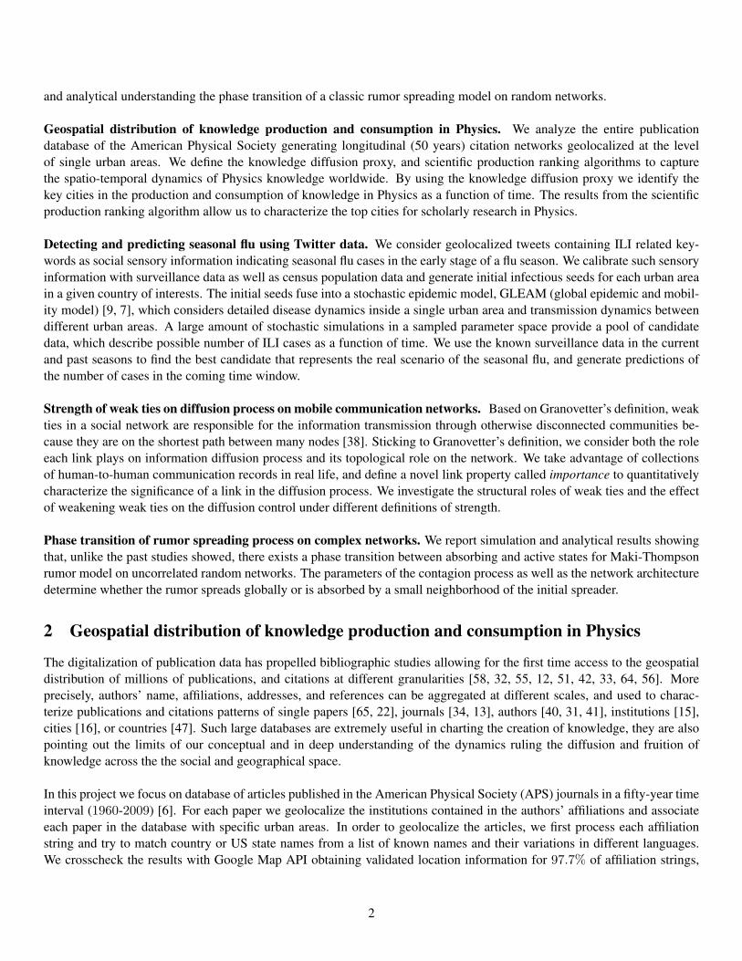
In Figure. 2.1-A and Figure. 2.1-B we visualize the results considering the Top four producer cities in 2009 in the USAand in Europe respectively. We show their Top ten consumers over 20 years as function of time. The size of each circle isproportional to how many times each injected citation is absorbed by that consumer. In the plot, vertical grey strips indicatethat the city was not a producer during those years (e.g. Orsay in 2008). The results show that, on average, Beijing is thetop consumer for all of these producers in the past 20 years. Since China registered a big economical growth and incrementof research population in the early 2000, it is reasonable to assume that, thanks to this positive stimulus, many more paperswere written in its capital, a dominant city for scientific research in China. However, the fast publication growth increased

3

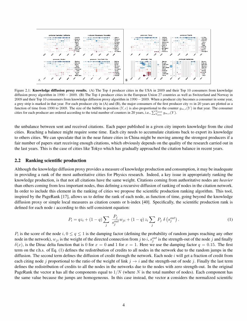
Figure 2.1: Knowledge diffusion proxy results. (A) The Top 4 producer cities in the USA in 2009 and their Top 10 consumers from knowledgediffusion proxy algorithm in 1990 − 2009. (B) The Top 4 producer cities in the European Union 27 countries as well as Switzerland and Norway in2009 and their Top 10 consumers from knowledge diffusion proxy algorithm in 1990− 2009. When a producer city becomes a consumer in some year,a grey strip is marked in that year. For each producer city in (A) and (B), the major consumers of the first producer city m in 20 years are plotted as afunction of time from 1990 to 2009. The size of the bubble in position (Y, c) is also proportional to the counter gm,c(Y ) in that year. The consumercities for each producer are ordered according to the total number of counters in 20 years, i.e.,

∑YmaxYmin

gm,c(Y ).

the unbalance between sent and received citations. Each paper published in a given city imports knowledge from the citedcities. Reaching a balance might require some time. Each city needs to accumulate citations back to export its knowledgeto others cities. We can speculate that in the near future cities in China might be moving among the strongest producers if afair number of papers start receiving enough citations, which obviously depends on the quality of the research carried out inthe last years. This is the case of cities like Tokyo which has gradually approached the citation balance in recent years.

2.2 Ranking scientific production

Although the knowledge diffusion proxy provides a measure of knowledge production and consumption, it may be inadequatein providing a rank of the most authoritative cities for Physics research. Indeed, a key issue in appropriately ranking theknowledge production, is that not all citations have the same weight. Citations coming from authoritative nodes are heavierthan others coming from less important nodes, thus defining a recursive diffusion of ranking of nodes in the citation network.In order to include this element in the ranking of cities we propose the scientific production ranking algorithm. This tool,inspired by the PageRank [17], allows us to define the rank of each node, as function of time, going beyond the knowledgediffusion proxy or simple local measures as citation counts or h-index [40]. Specifically, the scientific production rank isdefined for each node i according to this self-consistent equation:

Pi = qzi + (1− q)∑j

Pjsoutj

wji + (1− q) zi∑j

Pj δ(soutj

). (1)

Pi is the score of the node i, 0 ≤ q ≤ 1 is the damping factor (defining the probability of random jumps reaching any othernode in the network), wji is the weight of the directed connection from j to i, soutj is the strength-out of the node j and finallyδ(x), is the Dirac delta function that is 0 for x = 0 and 1 for x = 1. Here we use the damping factor q = 0.15. The firstterm on the r.h.s. of Eq. (1) defines the redistribution of credits to all nodes in the network due to the random jumps in thediffusion. The second term defines the diffusion of credit through the network. Each node i will get a fraction of credit fromeach citing node j proportional to the ratio of the weight of link j → i and the strength-out of node j. Finally the last termdefines the redistribution of credits to all the nodes in the networks due to the nodes with zero strength-out. In the originalPageRank the vector z has all the components equal to 1/N (where N is the total number of nodes). Each component hasthe same value because the jumps are homogeneous. In this case instead, the vector z considers the normalized scientific

4

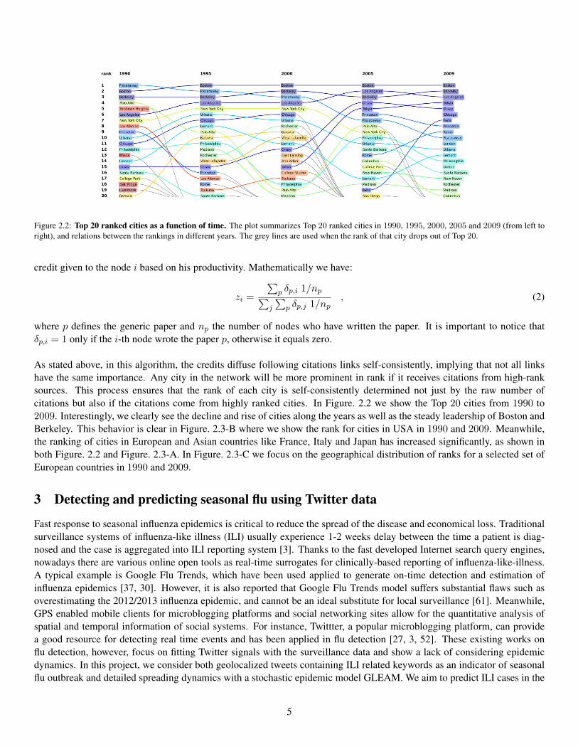
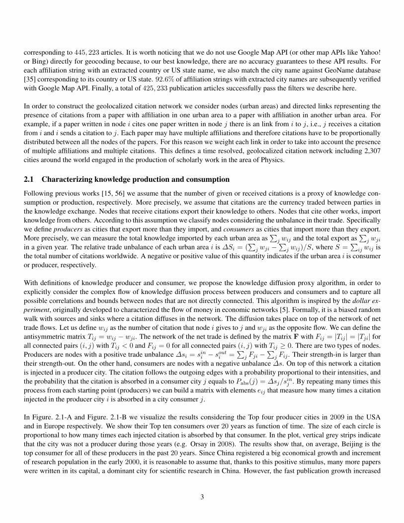
Figure 2.2: Top 20 ranked cities as a function of time. The plot summarizes Top 20 ranked cities in 1990, 1995, 2000, 2005 and 2009 (from left toright), and relations between the rankings in different years. The grey lines are used when the rank of that city drops out of Top 20.

credit given to the node i based on his productivity. Mathematically we have:

zi =

∑p δp,i 1/np∑

j

∑p δp,j 1/np

, (2)

where p defines the generic paper and np the number of nodes who have written the paper. It is important to notice thatδp,i = 1 only if the i-th node wrote the paper p, otherwise it equals zero.

As stated above, in this algorithm, the credits diffuse following citations links self-consistently, implying that not all linkshave the same importance. Any city in the network will be more prominent in rank if it receives citations from high-ranksources. This process ensures that the rank of each city is self-consistently determined not just by the raw number ofcitations but also if the citations come from highly ranked cities. In Figure. 2.2 we show the Top 20 cities from 1990 to2009. Interestingly, we clearly see the decline and rise of cities along the years as well as the steady leadership of Boston andBerkeley. This behavior is clear in Figure. 2.3-B where we show the rank for cities in USA in 1990 and 2009. Meanwhile,the ranking of cities in European and Asian countries like France, Italy and Japan has increased significantly, as shown inboth Figure. 2.2 and Figure. 2.3-A. In Figure. 2.3-C we focus on the geographical distribution of ranks for a selected set ofEuropean countries in 1990 and 2009.

3 Detecting and predicting seasonal flu using Twitter data

Fast response to seasonal influenza epidemics is critical to reduce the spread of the disease and economical loss. Traditionalsurveillance systems of influenza-like illness (ILI) usually experience 1-2 weeks delay between the time a patient is diag-nosed and the case is aggregated into ILI reporting system [3]. Thanks to the fast developed Internet search query engines,nowadays there are various online open tools as real-time surrogates for clinically-based reporting of influenza-like-illness.A typical example is Google Flu Trends, which have been used applied to generate on-time detection and estimation ofinfluenza epidemics [37, 30]. However, it is also reported that Google Flu Trends model suffers substantial flaws such asoverestimating the 2012/2013 influenza epidemic, and cannot be an ideal substitute for local surveillance [61]. Meanwhile,GPS enabled mobile clients for microblogging platforms and social networking sites allow for the quantitative analysis ofspatial and temporal information of social systems. For instance, Twittter, a popular microblogging platform, can providea good resource for detecting real time events and has been applied in flu detection [27, 3, 52]. These existing works onflu detection, however, focus on fitting Twitter signals with the surveillance data and show a lack of considering epidemicdynamics. In this project, we consider both geolocalized tweets containing ILI related keywords as an indicator of seasonalflu outbreak and detailed spreading dynamics with a stochastic epidemic model GLEAM. We aim to predict ILI cases in the

5

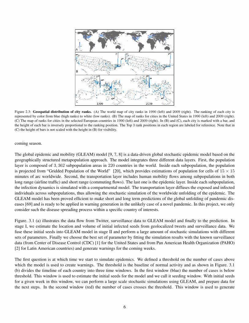
Figure 2.3: Geospatial distribution of city ranks. (A) The world map of city ranks in 1990 (left) and 2009 (right). The ranking of each city isrepresented by color from blue (high ranks) to white (low ranks). (B) The map of ranks for cities in the United States in 1990 (left) and 2009 (right).(C) The map of ranks for cities in the selected European countries in 1990 (left) and 2009 (right). In (B) and (C), each city is marked with a bar, andthe height of each bar is inversely proportional to the ranking position. The Top 3 rank positions in each region are labeled for reference. Note that in(C) the height of bars is not scaled with the height in (B) for visibility.

coming season.

The global epidemic and mobility (GLEAM) model [9, 7, 8] is a data-driven global stochastic epidemic model based on thegeographically structured metapopulation approach. The model integrates three different data layers. First, the populationlayer is composed of 3, 362 subpopulation areas in 220 countries in the world. Inside each subpopulation, the populationis projected from “Gridded Population of the World” [20], which provides estimations of population for cells of 15 × 15minutes of arc worldwide. Second, the transportation layer includes human mobility flows among subpopulations in bothlong range (airline traffic) and short range (commuting flows). The last one is the epidemic layer. Inside each subpopulation,the infection dynamics is simulated with a compartmental model. The transportation layer diffuses the exposed and infectedindividuals across subpopulations, thus allowing the stochastic simulation of the worldwide unfolding of the epidemic. TheGLEAM model has been proved efficient to make short and long term predictions of the global unfolding of pandemic dis-eases [69] and is ready to be applied in warning generation in the unlikely case of a novel pandemic. In this project, we onlyconsider such the disease spreading process within a specific country of interests.

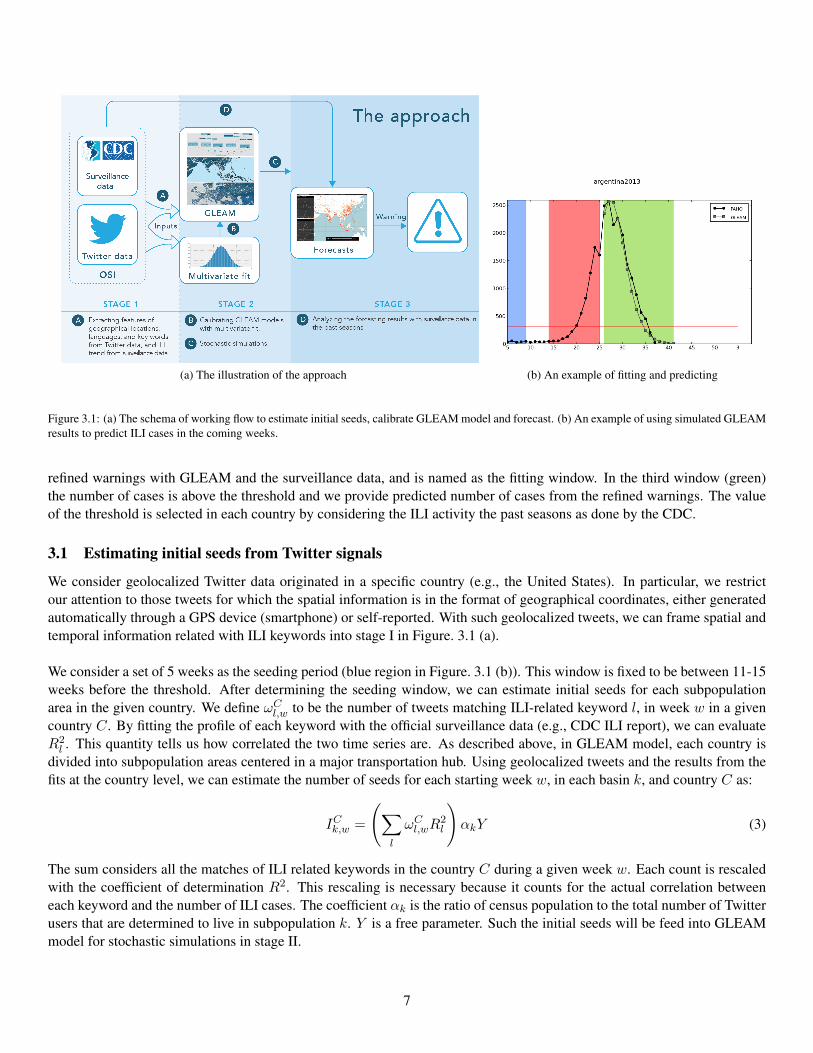
Figure. 3.1 (a) illustrates the data flow from Twitter, surveillance data to GLEAM model and finally to the prediction. Instage I, we estimate the location and volume of initial infected seeds from geolocalized tweets and surveillance data. Wefuse these initial seeds into GLEAM model in stage II and perform a large amount of stochastic simulations with differentsets of parameters. Finally we choose the best set of parameter by fitting the simulation results with the known surveillancedata (from Center of Disease Control (CDC) [1] for the United States and from Pan American Health Organization (PAHO)[2] for Latin American countries) and generate warnings for the coming weeks.

The first question is at which time we start to simulate epidemics. We defined a threshold on the number of cases abovewhich the model is used to create warnings. The threshold is the baseline of normal activity and as shown in Figure. 3.1(b) divides the timeline of each country into three time windows. In the first window (blue) the number of cases is belowthreshold. This window is used to estimate the initial seeds for the model and we call it seeding window. With initial seedsfor a given week in this window, we can perform a large scale stochastic simulations using GLEAM, and prepare data forthe next steps. In the second window (red) the number of cases crosses the threshold. This window is used to generate

6

(a) The illustration of the approach (b) An example of fitting and predicting

Figure 3.1: (a) The schema of working flow to estimate initial seeds, calibrate GLEAM model and forecast. (b) An example of using simulated GLEAMresults to predict ILI cases in the coming weeks.

refined warnings with GLEAM and the surveillance data, and is named as the fitting window. In the third window (green)the number of cases is above the threshold and we provide predicted number of cases from the refined warnings. The valueof the threshold is selected in each country by considering the ILI activity the past seasons as done by the CDC.

3.1 Estimating initial seeds from Twitter signals

We consider geolocalized Twitter data originated in a specific country (e.g., the United States). In particular, we restrictour attention to those tweets for which the spatial information is in the format of geographical coordinates, either generatedautomatically through a GPS device (smartphone) or self-reported. With such geolocalized tweets, we can frame spatial andtemporal information related with ILI keywords into stage I in Figure. 3.1 (a).

We consider a set of 5 weeks as the seeding period (blue region in Figure. 3.1 (b)). This window is fixed to be between 11-15weeks before the threshold. After determining the seeding window, we can estimate initial seeds for each subpopulationarea in the given country. We define ωCl,w to be the number of tweets matching ILI-related keyword l, in week w in a givencountry C. By fitting the profile of each keyword with the official surveillance data (e.g., CDC ILI report), we can evaluateR2l . This quantity tells us how correlated the two time series are. As described above, in GLEAM model, each country is

divided into subpopulation areas centered in a major transportation hub. Using geolocalized tweets and the results from thefits at the country level, we can estimate the number of seeds for each starting week w, in each basin k, and country C as:

ICk,w =

(∑l

ωCl,wR2l

)αkY (3)

The sum considers all the matches of ILI related keywords in the country C during a given week w. Each count is rescaledwith the coefficient of determination R2. This rescaling is necessary because it counts for the actual correlation betweeneach keyword and the number of ILI cases. The coefficient αk is the ratio of census population to the total number of Twitterusers that are determined to live in subpopulation k. Y is a free parameter. Such the initial seeds will be feed into GLEAMmodel for stochastic simulations in stage II.

7

3.2 Calibrating GLEAM and fitting surveillance data

Inside each subpopulation, the disease dynamics is modeled with a Susceptible-Latent-Infectious-Recovered (SLIR) com-partmental scheme, typical of ILI, where each individual has a discrete disease state assigned at each moment in time.Let β is the infection transmission rate and Ij/Nj is the density of infected individuals in the subpopulation j. Given theforce of infection λj = βIj/Nj , each person in the susceptible compartment (Sj) contracts the infection with probabilityλj∆t and enters the latent compartment (Lj), where ∆t is the time interval considered. Latent individuals exit the com-partment with probability ε∆t, and transit to asymptomatic infectious compartment (Iaj ) with probability pa or, with thecomplementary probability 1 − pa, become symptomatic infectious. Infectious persons with symptoms are further dividedbetween those who can travel (Itj), probability pt, and those who are travel-restricted (Intj ) with probability 1 − pt. All theinfectious persons permanently recover with probability µ∆t, entering the recovered compartment (Rj) in the next time step.

We then use GLEAM to perform a Latin Square Sampling in the parameter space w × Y × r, where w is the starting week,Y is the free parameter that rescales the initial number of cases, and r is the initial fraction of the immunized population.The simulation results of the models for each point in the sampled parameter space are compared with the real data in fittingwindow. This window, shown in red in Figure. 3.1 (b), is defined as the set of 12 weeks before the last data points of thesurveillance data. Once the best set of parameter is selected, the weeks above the threshold in the predicting window (green)are considered to generate warnings.

When using the this approach to predict the ongoing flu season there is a complication that does not affect studies of his-torical data. Indeed, the scale of the number of cases provided by surveillance data and by GLEAM is extremely different.It is necessary to rescale them in order to fit and generate warnings. In historical data this is a simple task: GLEAM datais rescaled by a factor x = max(GLEAM)/max(DATA). In the ongoing season the maximum (peak value) of the ILIcases in general may not be known, implying the impossibility of evaluating the rescaling factor x. If the surveillance datahave reached the peak in the current season, we apply the same technique as for historical data. If the data have not reachedthe peak value, we consider the average peak values in the past seasons. Since the peak value can be different from seasonto season, we also consider the standard deviation from the peak values in the past seasons. Formally the rescaling factorx = max(GLEAM)/(〈H〉+ kσ), where 〈H〉 is the average peak values in the past seasons for a given country, and we setk = −1, 0, 1, 2.

With rescaled GLEAM data for each point the sampled parameter space, we try to fit them with the surveillance data in thefitting window with different fitting methods. For each GLEAM candidate, we calculate the final fitting score s and selectthe one with the minimum value. s is defined as : s2 =

∑wi(di − gi)2, i = 0, . . . ,M − 1 where di is the real data and gi

is the rescaled GLEAM data in the week i. M is the fitting window size and i = 0 means the first week in the fitting region.The simplest method is unweighted fitting, where ∀i, wi = 1. This method treats all data points in the fitting region equally.However it is possible to argue that this is not the case. Indeed, getting better results in the last weeks, which are closer tothe green window, might be more important than reproducing perfectly the first weeks. In order to include this considerationin the fits we tested different choices assigning weights to each week in the red window giving more importance to the latestweeks. We tried two different weight functions. For exponential weighted fitting wi = e(i−10) and for linear weighted fittingwi = (i + 1)/10 if i < 10 else wi = 1. These two methods give more importance on the last two points in the fittingwindows. In Figure. 3.1 (b), we show an example of fitting and predicting for Argentina in season 2013. Suppose the lastdata point we have from the surveillance data is the week 25, and at the week 20 the surveillance data cross the threshold.The seeding window is week 5 to 9 and the fitting window is week 14 to 25. We rescale the GLEAM candidates with thepeak values of this season, and find the GLEAM candidate that best fits the surveillance data in the red window among allpoints in the sampled parameter space and with two weighted fitting methods.

8

3.3 Future works

The method we propose above can provide reasonable results for some countries with testing historical data. However thereare still some issues and some key factors that we have not taken into consideration and will be solved in the coming months.

I Currently we only use a list of ILI-related keywords to filter tweets. Some tweets containing these keywords might notindicate a single ILI case. For instance, if a news agency in a country tweets a news indicating an influenza outbreakin another country, and its followers can retweet the message. We now do not distinguish such tweets representingevents from the tweets indicating single cases. To better understand the tweet contents and get well defined indicators ofILI, we plan to filter tweets indicating real ILI cases with techniques of natural language processing, instead of simplycounting tweets containing keywords. We are trying to collect a random sample of tweets in the past seasons with atleast one ILI-related keyword. With this sample, we are going to do human-annotating to get a training set of tweetsrepresenting single ILI case. With the trained dataset we plan to use the n-gram model classifying tweets.

II In the very early stage in a seasonal flu season, tweets containing ILI related keywords might be very random andmay not reflect the real spatial distribution of initial seeds. Besides, we found that the final parameter set for the bestfitted GLEAM simulation is not sensitive to the initial weeks. In order to get better estimation of initial conditions forGLEAM model, we plan to select the starting week of simulations to be two weeks before the surveillance data crossthe baseline.

III We fixed the basic reproduction number R0 = 1.75 in GLEAM model at the present time. R0 for seasonal influenzamight change from season to season, e.g., for the United States it varies from 0.9 to 2.1 [23]. We plan to perform moresimulations and analysis with different values of R0 and test the sensitivity of results to such model parameters.

IV Besides the ILI reporting at the country level, CDC also collects data for nine census regions. Weekly updates arealso issued at regional granularities. Such high-resolution data provide an opportunity to test predictions at differentgeographical resolution. We are planning to apply the above approach to different regional datasets and aggregate tothe country level. With this approach we will be able to test the geographical role that Twitter signals play at differentspatial granularities.

4 Strength of weak ties on diffusion process on mobile communication networks

Beyond various studies on the dynamics of diffusion processes on complex networks [11], recent works on studying diffusionprocess on social networks have recourse to the traditional concepts in sociology, like weak ties [63, 73, 43]. According to[38], local bridges in a social network are responsible for the information transmission through the embedded communitiesand play a crucial role in information diffusion between otherwise disconnected communities since they are on the shortestpath between many nodes [38, 39]. All of these bridges are weak ties, and the significance of weak ties is the local bridgecreating more and shorter path [38]. Such definition of weak ties provides better understandings of how micro-interactionbehavior translating into macro-patterns of a social system [38].

Thanks to the emergence of large datasets of human-to-human interactions, the strength of links on real large-scale socialsystems such as mobile communication networks and online social networks has been measured quantitatively with variousdefinitions: overlap [62, 73], the number of calls, the maximum inter-event time between two individuals [44, 43], etc. Thesemeasurements consider either topological features of the static network or temporal patterns of events. These past studiesconfirm that weak ties help slowing down the spreading process [63] and the dynamical processes are not necessarily topo-logically efficient because of weight-topology correlation and burstiness of individuals [44]. Meanwhile it also reported thatthe strength of weak ties does not help the diffusion process of complex contagions [21, 73, 36]. However until now thereis still no agreement on what is a “weak tie”. In this study, we go back to the original Granovetter’s definition of weak tie,and consider both the role each link plays on information diffusion process and its topological role on the network. We take

9

advantage of collections of human-to-human communication records in real life, and use an information propagation modelto find out how important a link is in the dissemination process.

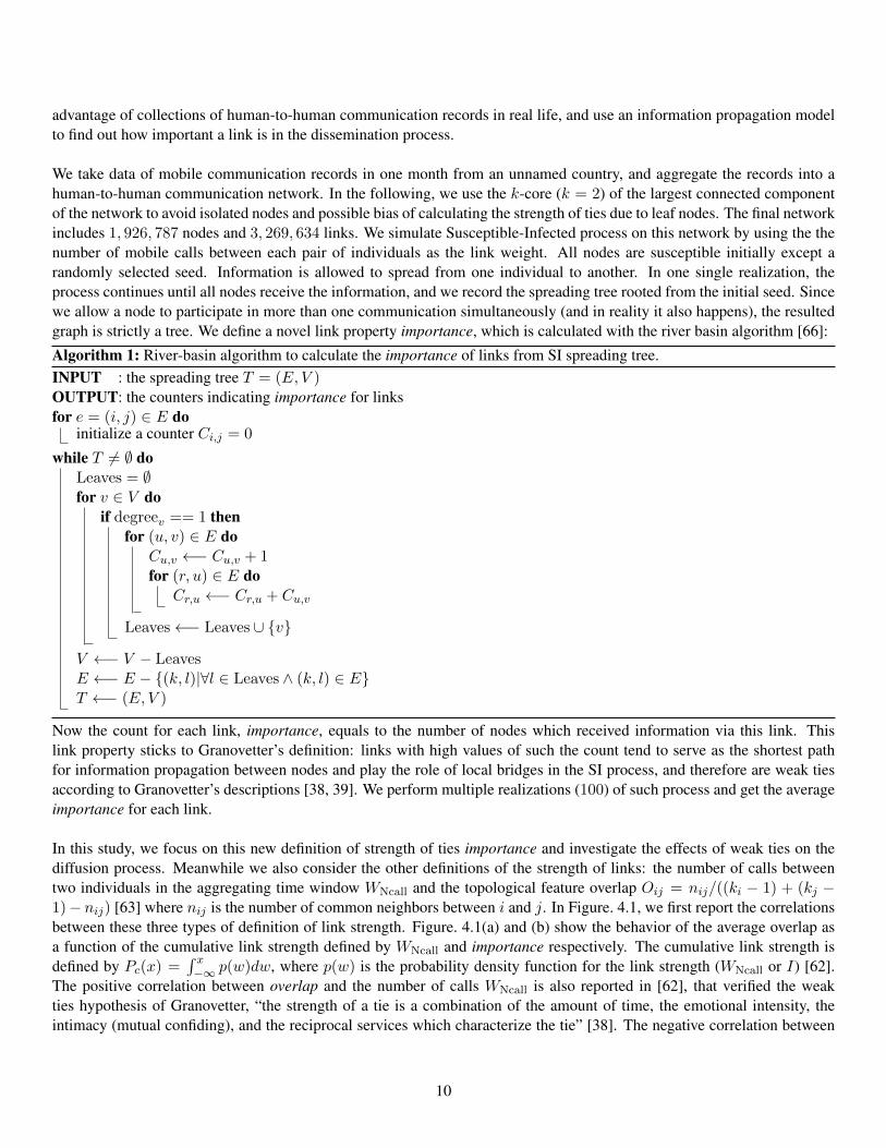
We take data of mobile communication records in one month from an unnamed country, and aggregate the records into ahuman-to-human communication network. In the following, we use the k-core (k = 2) of the largest connected componentof the network to avoid isolated nodes and possible bias of calculating the strength of ties due to leaf nodes. The final networkincludes 1, 926, 787 nodes and 3, 269, 634 links. We simulate Susceptible-Infected process on this network by using the thenumber of mobile calls between each pair of individuals as the link weight. All nodes are susceptible initially except arandomly selected seed. Information is allowed to spread from one individual to another. In one single realization, theprocess continues until all nodes receive the information, and we record the spreading tree rooted from the initial seed. Sincewe allow a node to participate in more than one communication simultaneously (and in reality it also happens), the resultedgraph is strictly a tree. We define a novel link property importance, which is calculated with the river basin algorithm [66]:

Algorithm 1: River-basin algorithm to calculate the importance of links from SI spreading tree.INPUT : the spreading tree T = (E, V )OUTPUT: the counters indicating importance for linksfor e = (i, j) ∈ E do

initialize a counter Ci,j = 0

while T 6= ∅ doLeaves = ∅for v ∈ V do

if degreev == 1 thenfor (u, v) ∈ E do

Cu,v ←− Cu,v + 1for (r, u) ∈ E do

Cr,u ←− Cr,u + Cu,v

Leaves←− Leaves ∪ {v}

V ←− V − LeavesE ←− E − {(k, l)|∀l ∈ Leaves ∧ (k, l) ∈ E}T ←− (E, V )

Now the count for each link, importance, equals to the number of nodes which received information via this link. Thislink property sticks to Granovetter’s definition: links with high values of such the count tend to serve as the shortest pathfor information propagation between nodes and play the role of local bridges in the SI process, and therefore are weak tiesaccording to Granovetter’s descriptions [38, 39]. We perform multiple realizations (100) of such process and get the averageimportance for each link.

In this study, we focus on this new definition of strength of ties importance and investigate the effects of weak ties on thediffusion process. Meanwhile we also consider the other definitions of the strength of links: the number of calls betweentwo individuals in the aggregating time window WNcall and the topological feature overlap Oij = nij/((ki − 1) + (kj −1)− nij) [63] where nij is the number of common neighbors between i and j. In Figure. 4.1, we first report the correlationsbetween these three types of definition of link strength. Figure. 4.1(a) and (b) show the behavior of the average overlap asa function of the cumulative link strength defined by WNcall and importance respectively. The cumulative link strength isdefined by Pc(x) =

∫ x−∞ p(w)dw, where p(w) is the probability density function for the link strength (WNcall or I) [62].

The positive correlation between overlap and the number of calls WNcall is also reported in [62], that verified the weakties hypothesis of Granovetter, “the strength of a tie is a combination of the amount of time, the emotional intensity, theintimacy (mutual confiding), and the reciprocal services which characterize the tie” [38]. The negative correlation between

10

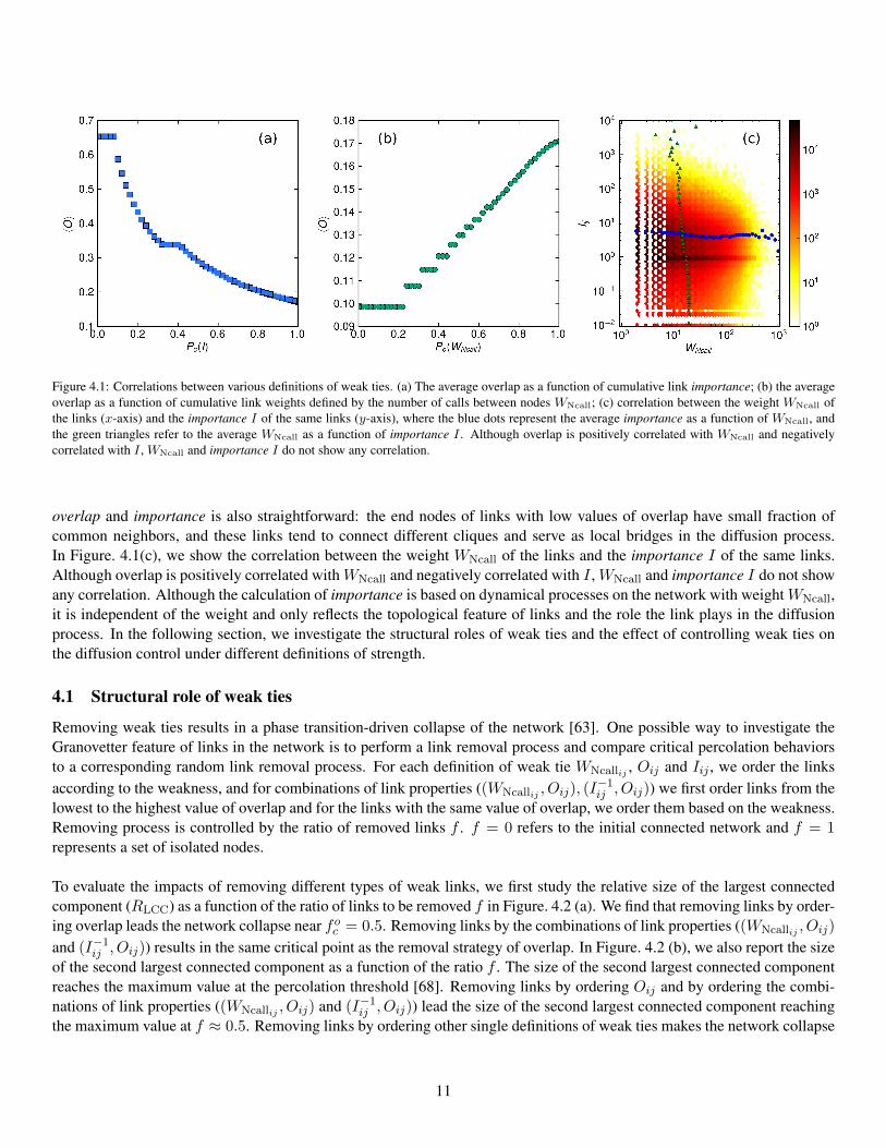
Figure 4.1: Correlations between various definitions of weak ties. (a) The average overlap as a function of cumulative link importance; (b) the averageoverlap as a function of cumulative link weights defined by the number of calls between nodes WNcall; (c) correlation between the weight WNcall ofthe links (x-axis) and the importance I of the same links (y-axis), where the blue dots represent the average importance as a function of WNcall, andthe green triangles refer to the average WNcall as a function of importance I . Although overlap is positively correlated with WNcall and negativelycorrelated with I , WNcall and importance I do not show any correlation.

overlap and importance is also straightforward: the end nodes of links with low values of overlap have small fraction ofcommon neighbors, and these links tend to connect different cliques and serve as local bridges in the diffusion process.In Figure. 4.1(c), we show the correlation between the weight WNcall of the links and the importance I of the same links.Although overlap is positively correlated withWNcall and negatively correlated with I , WNcall and importance I do not showany correlation. Although the calculation of importance is based on dynamical processes on the network with weightWNcall,it is independent of the weight and only reflects the topological feature of links and the role the link plays in the diffusionprocess. In the following section, we investigate the structural roles of weak ties and the effect of controlling weak ties onthe diffusion control under different definitions of strength.

4.1 Structural role of weak ties

Removing weak ties results in a phase transition-driven collapse of the network [63]. One possible way to investigate theGranovetter feature of links in the network is to perform a link removal process and compare critical percolation behaviorsto a corresponding random link removal process. For each definition of weak tie WNcallij , Oij and Iij , we order the linksaccording to the weakness, and for combinations of link properties ((WNcallij , Oij), (I

−1ij , Oij)) we first order links from the

lowest to the highest value of overlap and for the links with the same value of overlap, we order them based on the weakness.Removing process is controlled by the ratio of removed links f . f = 0 refers to the initial connected network and f = 1represents a set of isolated nodes.

To evaluate the impacts of removing different types of weak links, we first study the relative size of the largest connectedcomponent (RLCC) as a function of the ratio of links to be removed f in Figure. 4.2 (a). We find that removing links by order-ing overlap leads the network collapse near foc = 0.5. Removing links by the combinations of link properties ((WNcallij , Oij)

and (I−1ij , Oij)) results in the same critical point as the removal strategy of overlap. In Figure. 4.2 (b), we also report the sizeof the second largest connected component as a function of the ratio f . The size of the second largest connected componentreaches the maximum value at the percolation threshold [68]. Removing links by ordering Oij and by ordering the combi-nations of link properties ((WNcallij , Oij) and (I−1ij , Oij)) lead the size of the second largest connected component reachingthe maximum value at f ≈ 0.5. Removing links by ordering other single definitions of weak ties makes the network collapse

11

(a) The relative size of the largest connected component (b) The size of the second largest connected component

Figure 4.2: Percolation study: Global quantities of the network as a function of the ratio of links to be removed f .

at fc > 0.5. If links are removed according to the weakness defined by importance, f Ic ≈ 0.56 . Meanwhile, removinglinks that ordered by the number of calls disintegrates the network at fWNcall

c ≈ 0.75, close to the critical value for randomremoving links.

In Figure. 4.2 (a-II) we observe that the network collapses faster if links are ordered by the combinations (I−1ij , Oij) and(WNcallij , Oij) than removing links ordered by overlap alone when the fraction of removed links is between 0.2 to 0.48.From the perspective of percolation, the link property overlap determines the critical point of the phase transition. A linkwith Oij = 0 indicating the nodes it connects has no common neighbors, and connects different social cliques or localcommunities. In the sample of mobile call network we investigate, there are around 48% of links with Oij = 0. Removingall of these links disintegrates the network into a set of cliques. Removing links by ordering the combinations of weaknessproperties of link does not change the percolation threshold but speeds up the network collapsing, i.e., removing a fractionof links f < 0.48 results in the smaller size of the largest connected component.

4.2 Diffusion role of weak ties

In information spreading process, such weak ties with Oij = 0 enhance the trapping effect inside local clusters, and slowdown diffusion process between clusters [62]. Controlling these weak ties could further impede the spreading. For instance,in the case of rumor spreading in a communication network or infectious disease spreading in a contagion network, onecould expect to weaken the strength of a small fraction of links to impede the propagations. Further identifying weak ties

12

among these zero overlap links could reduce the amount of links to be controlled. In this section, we turn into investigatingthe effects of controlling weak links under various definitions on diffusion processes to study how much we can control thecontagion by decreasing the transmission probabilities on weak ties.

From the results above, removing links by ordering their property combinations (WNcallij , Oij) or (I−1ij , Oij) results in net-work collapsing faster than other definitions of weakness when the fraction of links removed is between 0.2 and 0.48. Toimpede the diffusion process of rumor or infectious disease, one could decrease the probabilities of contagion between twonodes between the weak link by weakening their connection weight. SIR model is well known for studying dynamics of epi-demics [4] and rumor spreading [59]. In the following we apply SIR model on the communication network and control weak

ties defined by the combinations of link properties by weakening the weights of links. Consider the SIR system S+ Iβ→ 2I ,

Iµ→ R. The final size of epidemic R refers to the total recovered population size. We fixed the infection rate β = 0.25 and

the recovery rate µ = 0.1. The recovery rate µ is constant for each individual in the network. However, the probability of anindividual i to be infected by contacting j is pij ∝ wijβ. On the unweighted network wij = 1, and on the weighted networkwij is defined based on the number of calls between the two nodes (WNcall).

We first focus on the unweighted network. Similarly to the percolation study, for a given percentage of links f , we or-der the first f links based on the combination of link properties (I−1ij , Oij), and we scale the link weights wij from 1 toδ, (0 < δ ≤ 1). As a control experiment, we randomly choose the same percentage of links f , and scale the link in the sameway. We compare the final size of epidemic in these two cases by measuring R(I−1,O)/Rrandom as a function of the scalingfactors δ for different values of f . If controlling weak ties performs as the same as the random links, this ratio is 1.0. If itis more efficient, the ratio should be less than 1.0. In Figure. 4.3 (a) top panel (solid lines), we show such the comparisonresults. When δ ≤ 0.1, weakening the weights on weak ties reduces at least 50% of the final size of epidemic than weakeningthe weights on random links.

In the same figure, instead of (I−1ij , Oij), we control weak ties that are defined by the (WNcallij , Oij) and measure the samequantities for different values of f (dashed lines in Figure. 4.3 (a) top panel). Since there are around 48% links with Oij = 0the effects of controlling weak ties of these two definitions are similar. When f = 36%, controlling weak ties defined by(I−1ij , Oij) reduces the final size of epidemic more than 60% with the scaling factor δ = 0.01. When f = 12%, the effectsof controlling weak ties by these two definitions are also similar.To further compare the effects of controlling ties of these two definitions ((WNcallij , Oij) and (I−1ij , Oij)) on spreadingdynamics, we report R(I−1,O)/R(WNcallij

,Oij) as a function of the fraction of controlled links f for a given δ = 0.01 in

Figure. 4.3 (a) bottom panel. When 0.24 < f < 0.48, one can observe controlling weak ties defined by (I−1ij , Oij) resultssignificantly less infected population than by (WNcallij , Oij). This result is consistent with the observation in percolationstudy, that when f is between 0.25 and 0.45, the largest connected component is smaller if removing links are ordered by(I−1ij , Oij). Controlling weak ties defined by (I−1ij , Oij) limits the infected population inside a smaller community.

We also perform the same experiments on the weighted mobile communication network. The weight between node i andnode j is defined as wij = WNCall

ij /〈WNCall〉 if WNCallij ≤ 〈WNCall〉, and wij = 1 if WNCall

ij > 〈WNCall〉, where WNCallij

is the number of calls between node i and node j and 〈WNCall〉 is the average number of calls among all pairs of individualsin the network. Figure. 4.3 (b) top panel shows the ratio R(I−1,O)/Rrandom as a function of the scaling factor δ for the SIRprocess on the weighted network. The results are similar to the unweighted case. For example, at δ = 0.01, controlling 12%of weak ties defined by R(I−1,O) leads to 60% less infected population than randomly controlling the same fraction of links.When f = 24% and above the final size of epidemic reduces more than 90% than controlling with the random strategy forδ < 0.1. Similar to the unweighted case, we also report R(I−1,O)/R(WNcallij

,Oij) as a function of the fraction of controlledlinks f for a given δ = 0.01 in the bottom panel in Figure. 4.3 (b). When 0.18 < f < 0.48, controlling weak ties definedby (I−1ij , Oij) results at least 80% less infected population than controlling weak ties defined by (WNcallij , Oij). Althoughthe quantitative results vary, the qualitative behaviors in the experiments on both unweighted and weighted networks are

13

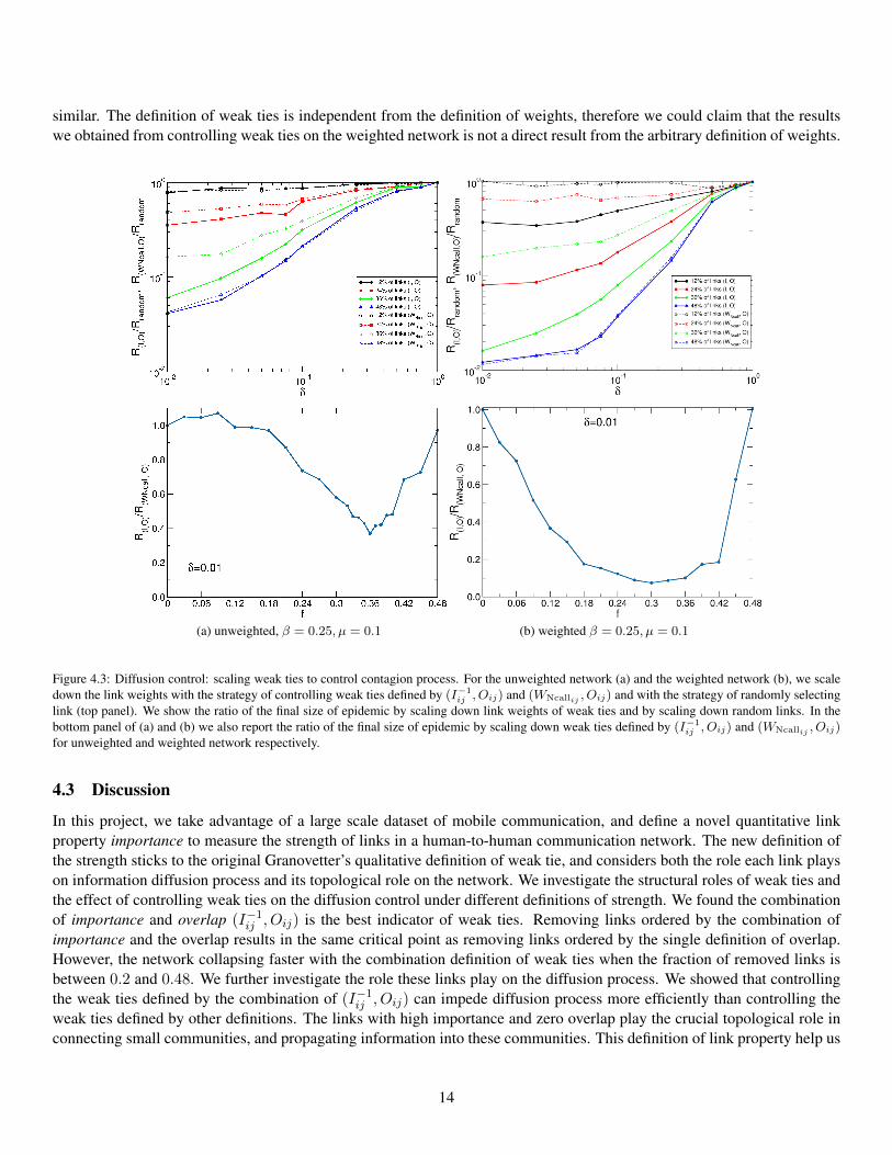
similar. The definition of weak ties is independent from the definition of weights, therefore we could claim that the resultswe obtained from controlling weak ties on the weighted network is not a direct result from the arbitrary definition of weights.

(a) unweighted, β = 0.25, µ = 0.1 (b) weighted β = 0.25, µ = 0.1

Figure 4.3: Diffusion control: scaling weak ties to control contagion process. For the unweighted network (a) and the weighted network (b), we scaledown the link weights with the strategy of controlling weak ties defined by (I−1

ij , Oij) and (WNcallij , Oij) and with the strategy of randomly selectinglink (top panel). We show the ratio of the final size of epidemic by scaling down link weights of weak ties and by scaling down random links. In thebottom panel of (a) and (b) we also report the ratio of the final size of epidemic by scaling down weak ties defined by (I−1

ij , Oij) and (WNcallij , Oij)for unweighted and weighted network respectively.

4.3 Discussion

In this project, we take advantage of a large scale dataset of mobile communication, and define a novel quantitative linkproperty importance to measure the strength of links in a human-to-human communication network. The new definition ofthe strength sticks to the original Granovetter’s qualitative definition of weak tie, and considers both the role each link playson information diffusion process and its topological role on the network. We investigate the structural roles of weak ties andthe effect of controlling weak ties on the diffusion control under different definitions of strength. We found the combinationof importance and overlap (I−1ij , Oij) is the best indicator of weak ties. Removing links ordered by the combination ofimportance and the overlap results in the same critical point as removing links ordered by the single definition of overlap.However, the network collapsing faster with the combination definition of weak ties when the fraction of removed links isbetween 0.2 and 0.48. We further investigate the role these links play on the diffusion process. We showed that controllingthe weak ties defined by the combination of (I−1ij , Oij) can impede diffusion process more efficiently than controlling theweak ties defined by other definitions. The links with high importance and zero overlap play the crucial topological role inconnecting small communities, and propagating information into these communities. This definition of link property help us

14

gaining a better understanding of the weak ties in human-to-human communication networks.

5 Phase transition of rumor spreading process on complex networks

In order to study information diffusion on complex contact networks we have considered the rumor model by Maki andThompson [53]. The model defines three exclusive states or compartments for each individual: ignorant (I), spreader (S)and stifler (R). Ignorants are those individuals who have not heard the rumor yet. While both the spreaders and stiflers haveheard the rumor, only the spreaders wish to spread it. The number of ignorants I(t), spreaders S(t) and stiflers R(t) at timet hence constitute the state variables of the system. An ignorant hears the rumor from a spreader neighbor and becomes aspreader herself at rate λ. Each spreader becomes a stifler, hence, stops spreading the rumor either by a spreader or a stiflercontact at rate α. This set of rules defines a reaction or diffusion process in which I + S

λ→ 2S, S + Sα→ R + S and

S+Rα→ 2R. In the absence of demographic changes the total population size N is conserved and N = I(t) +S(t) +R(t).

In the discussion below i(t), s(t) and r(t) refer to the prevalence of ignorant, spreader and stifler individuals in the popula-tion, respectively.

While the above dynamics is reminiscent of the well-known Susceptible-Infected-Recovered epidemic model [46], it has asubtle difference. Unlike the epidemic model, the rumor model does not possess a spreading threshold when the populationis fully mixed, i.e., each individual is capable of contacting any other individual in the population. This means that wheneverthe spreading rate λ is nonzero, the rumor spreads to a finite fraction of the population in thermodynamic limit N →∞.

The original study by Moreno et al. [57] focusing on contact networks, where each individual has a fixed set of neighbors,has also concluded that the same is valid in homogeneous contact networks. However, the analytical approach taken in thestudy [57] is based on a Mean-Field assumption unable to tackle the quenched nature of connections. The availability oflarge-scale datasets on communication networks in recent years [62, 50, 48, 18, 49], however, presents new opportunities forthe study of information dissemination in social networks and the utility of rumor models [53, 28]. In this project, we reportnumerical and analytical evidences that the parameters of the rumor contagion process and the architecture of connectionsdetermine whether a new rumor spreads globally in social networks.

5.1 Results from Monte Carlo simulations

To easily compare simulation results and analytical calculations, we consider uncorrelated random networks [19] in whicheach of N nodes has the same number k of connections. We generate at least 10 random networks with k = 7 for eachpopulation size N varying between 103 and 106. We fix the annihilation rate α at 0.5 and vary the spreading rate λ. Foreach set of parameters we perform at least 103 realizations of the rumor contagion process on each synthetic network. Eachdynamical realization starts with a fully ignorant population except for one randomly chosen node turning into a spreader andruns until no spreader is left in the network. During the time step between t and t + 1, a spreader at time t contacts or callsall her immediate neighbors one by one. If the recipient is an ignorant at time t, the ignorant neighbor becomes a spreaderat time t + 1 with probability λ. If the recipient is a spreader or stifler instead, the caller becomes a stifler at time t + 1with probability α. In order to let the model be analytically tractable we do not impose any memory in the communicationsduring a time step. Hence if a spreader calls another spreader, the callee turns into a stifler at time t+ 1 with probability α,independent of the status change of the caller.

15

Figure 5.1: Monte Carlo simulation results (the results are obtained by averaging over 10 × 103 realizations, corresponding to 10 network realizationsand 103 rumor contagion processes on each one of them) and numerical solution to analytic results. (A) The final prevalence of the rumor r∞ as afunction of the spreading rate λ for different population sizes N = 103 (black dots), N = 104 (red squares), N = 105 (green diamond) and N = 106

(blue triangles). The annihilation rate and the node degrees are fixed at α = 0.5 and k = 7, respectively. The inset is a zoom of the transition region.(B) Probability distribution of the final rumor size R∞ for N = 105, α = 0.5, and k = 7. Different symbols correspond to different values of thespreading rate: λ = 0.05 (blue circles), λ = 0.1 (red squares), λ = 0.11 (green pluses) and λ = 0.15 (brown diamonds). The solid line correspondsto the power-law function with exponent −1.44 plotted for comparison with the distribution for λ = 0.1. (C, D) Finite-size scaling and data collapse.(C) The final rumor prevalence r∞ as a function of population size N for different values of λ. The dashed-dotted, dashed, dotted and solid linescorrespond to the power-law fits with the exponent −1, −0.99, −0.92 and −0.59, respectively. (D) The best data collapse of the final rumor prevalencer∞ obtained at βν = 0.59, ν = 0.35 and λc = 0.1. (E) The final prevalence of rumor r∞ as a function of the spreading rate λ for the population sizeN = 105 on the quenched random network with (red dots) and on the corresponding annealed networks (blue squares). The solid line corresponds tothe Mean-Field solution obtained from Eqs. 5–7 numerically. (F) Phase space of the rumor model on the λ–α plane for k = 7. The line separating theactive and absorbing phases corresponds to n∞ = 1 and is obtained by solving Eqs. 10 and 13 numerically.

In Figure. 5.1 (A) we show the final prevalence of rumor r∞ as a function of the spreading rate λ for different populationsizes. We observe that when λ is smaller than about 0.1, the final prevalence of rumor r∞ depends on the population sizeN . In contrast, when λ is larger, r∞ is independent of N . The probability distribution of the final rumor size R∞ fordifferent values of λ, illustrated in Figure. 5.1 (B), shows the power-law distribution of the final rumor size for λ = 0.1.When λ = 0.05, the distribution decays exponentially. For λ = 0.11 and 0.15, the distributions are bimodal in that mostof the realizations yields global rumor spread. All of these features are fingerprints of critical phenomena and imply theexistence of non-equilibrium phase transitions in rumor model as the parameter space is explored. In the region of λ� 0.1the spreading rate is much lower than the annihilation rate, and an early spreader loses her interest in the rumor much quickerthan she can spread it. Thus the rumor is heard by a small number of early spreaders only, and the final size of rumor R∞does not scale with population size, i.e., the final prevalence of rumor r∞ ∝ N−1. In the second region of λ � 0.1, therumor can reach a large number of indivuduals because of the relatively large spreading rate combined with the number ofconnections. The final size of rumor in this region is proportional to the population size, i.e., r∞ is independent of N .Right above the critical point λc, the order parameter r∞ obeys the scaling law r∞ ∝ (λ− λc)β [54]. In order to determineλc and β, we perform finite-size scaling analysis [54, 60]. In Figure. 5.1 (C), we show the final prevalence of rumor r∞ asa function of population sizes N for λ values in the vicinity of 0.1. For λ = 0.085, 0.09 and 0.095, we find approximatelyr∞ ∝ N−1. When λ = 0.105 and 0.11, the rumor reaches a finite fraction of the population that is independent of the

16

population size. These findings imply that the system is in a subcritical regime for λ < 0.1 and is supercritical whenλ > 0.1. At λ = 0.1, r∞ ∝ N−ρ where ρ = 0.59 ± 0.02, and we get the estimation of λc = 0.1 ± 0.005. Following thefinite-size scaling method [60]

r∞Nβν = F ((λ− λc)Nν) , (4)

where F (•) is the scaling function, and r∞ = F (0)N−βν at λ = λc. As discussed above, ρ = βν = 0.59 ± 0.02.In Figure. 5.1 (D) we display the best data collapse obtained for ν = 0.35 ± 0.01 in the vicinity of λc = 0.1, yieldingβ = 1.68± 0.01.

The simulations show that the rumor propagation gets confined to a small neighborhood of early spreaders if the spreadingrate is much smaller than the annihilation rate. This result is in contradiction with the previous studies [57] based on a Mean-Field approximation. As already stated earlier, the Mean-Field approximation considers an ensemble of annealed randomnetworks [29, 14]. This means that the links are re-established while the degree distribution is kept invariant. In such anensemble, every node has the potential of contacting every other node in the population during the course of a dynamicalprocess running on top. The Mean-Field rate equations describing the prevalences of compartments over time are thenroughly given by

i′(t) = −i(t)[1− (1− λs(t))k] , (5)

s′(t) = i(t)[1− (1− λs(t))k]− s(t)[1− [1− α(s(t) + r(t))]k] , (6)

r′(t) = s(t)[1− [1− α(s(t) + r(t))]k] , (7)

with the constraint i(t) + s(t) + r(t) = 1. When λ and α are sufficiently small, the above equations are equivalent to theMean-Field equations in [57].

In Figure. 5.1 (E) we report the simulation results of rumor propagation dynamics on annealed random networks of sizeN = 105. The simulations on annealed networks agree with the numerical solutions of the Mean-Field Eqs. 5–7, both ofwhich are strikingly different from the simulations on quenched networks. The simulations on annealed networks have beenperformed by reshuffling all the edges at the end of each time step of the rumor dynamics. The reshuffling process enablesearly spreaders to keep their interests in the rumor and spread it to different neighborhoods until a sufficiently large numberof individuals hear the rumor.

5.2 Analytic results

By definition of the rumor model, the initial spreader has to pass the rumor to a neighbor in order to enable the annihila-tion process. However, as the above simulation results imply, the outreach of the rumor on quenched contact networks isdetermined by the network structure and the spreading and annihilation rates. We may tackle the problem analytically byconsidering the immediate social network of an early spreader, hence, the ego network. Consider the moment at which theego has x ignorant neighbors only among her k neighbors in total, hence, k − x of her neighbors are either spreaders orstiflers. During the next time step the ego spreads the rumor to 0 ≤ n ≤ x ignorant neighbors and either loses her interestin the rumor or keeps her status as spreader. The probabilities of encountering these two events pk and qk, respectively, aregiven by

pk(n|x) =

(x

n

)λn(1− λ)x−n(1− α)k−x , (8)

qk(n|x) =

(x

n

)λn(1− λ)x−n

[1− (1− α)k−x

]. (9)

In order to answer the question concerning the global rumor spread, we need to consider the whole period in which the egois a spreader. If an early spreader can spread the rumor to at least one ignorant neighbor on average, then the rumor may

17

have a global outreach.

Suppose that only the x0 of k neighbors are ignorant at the moment when the ego’s status turns into a spreader, and denote theprobability that the ego spreads the rumor to n∞ neighbors during her spreader period by Pk(n∞|x0). The average numberof newly generated spreaders by an early spreader, i.e., x0 = k − 1, is then

n∞ =

k−1∑n=0

nPk(n|k − 1) . (10)

If n∞ ≥ 1, then the rumor stays alive in the early stages of the contagion dynamics and be propagated globally. The rumor isgoing to be confined to a small neighborhood if n∞ < 1. It is worth remarking that the threshold parameter n∞ is equivalentto the so-called basic reproduction number in epidemic processes [45]. The basic reproduction number is the average totalnumber of secondary infections generated by an infectious person in the early stages of the epidemics. Equivalently here,n∞ is the average total number of spreaders generated by a spreader during the early stages of the rumor dynamics.

While finding a closed form of the probability Pk(n|x) is not a piece of cake, we can write down an expression that canthen be computed numerically. Let us write down the expressions for n = 1 in order to demonstrate the logic here. Theprobability of spreading the rumor to one neighbor only is

Pk(1|k − 1) =∞∑t1=0

[pk(0|k − 1)]t1

[qk(1|k − 1) + pk(1|k − 1)

∞∑t2=0

[pk(0|k − 2)]t2qk(0|k − 2)

], (11)

where t1 + 1 counts the number of time steps from the moment when the ego becomes spreader till the end of the time stepduring which the rumor is propagated to one neighbor successfully. The ego may become a stifler during the same timestep. If the ego is still a spreader, t2 counts the number of time steps proceeding the generation of the new spreader until theannihilation of the ego. We may easily perform the summations over the dummy variables t1 and t2 as these are just sums ofgeometric series, yielding

Pk(1|k − 1) =1

1− pk(0|k − 1)

[qk(1|k − 1) + pk(1|k − 1)

qk(0|k − 2)

1− pk(0|k − 2)

]. (12)

We follow the same logic above in order to express the probability of spreading the rumor to an arbitrary number n ofneighbors in total. The ego may generate all the n spreaders at once and become a stifler herself or survive for an additionalperiod. The ego may spread the rumor to n1 > 0 and n − n1 > 0 ignorant neighbors sequentially. She may change herstatus during the last generation or survive a bit longer before losing her interest in the rumor. The ego can generate n1 > 0,n2 > 0 and n− n1 − n2 > 0 new spreaders sequentially. During the time step of the generation of the last group with sizen − n1 − n2, she may become a stifler or keeps her interest in the rumor for an additional period. This continues until thelast configuration in which each new spreader is generated sequentially. One may consider this sequence of events as theconfigurations of having n balls grouped into 1 ≤ b ≤ n boxes, each of which containing at least one ball, and a ‘stop’ signaligned on the timeline. The ‘stop’ sign can be located only at/after the position of the last box on the timeline. Each ballcorresponds to an ignorant neighbor who eventually hears the rumor from the ego, and each box to a time step during whichthe ego spreads the rumor to a certain number of ignorant neighbors. The stop sign is the event of successful annihilation.Considering all the configurations, the probability that the ego generates n new spreaders only during her spreader period is

18

given by Eq. 13:

Pk(n|k − 1) =1

1− pk(0|k − 1)

[qk(n|k − 1) + (1− δn,0)pk(n|k − 1)

qk(0|k − 1− n)

1− pk(0|k − 1− n)

]+ (1− δn,0)(1− δn,1)

n−1∑n1=1

pk(n1|k − 1)

1− pk(0|k − 1)× 1

1− pk(0|k − 1− n1)

[qk(n− n1|k − 1− n1)

+ pk(n− n1|k − 1− n1)qk(0|k − 1− n)

1− pk(0|k − 1− n)

]+ (1− δn,0)(1− δn,1)(1− δn,2)

n∑b=3

∑{ni}

′ pk(n1|k − 1)

1− pk(0|k − 1)×b−1∏i=2

pk(ni|k − 1−∑i−1

j=1 nj)

1− pk(0|k − 1−∑i−1

j=1 nj)

× 1

1− pk(0|k − 1−∑b−1

j=1 nj)

qk(nb|k − 1−b−1∑j=1

nj) + pk(nb|k − 1−b−1∑j=1

nj)qk(0|k − 1− n)

1− pk(0|k − 1− n)

,(13)

where nb = n−∑b−1

j=1 nj and

∑{ni}

′≡

n−b+1∑n1=1

. . .

n−b+i−∑i−1

j=1 nj∑ni=1

. . .

n−1−∑b−2

j=1 nj∑nb−1=1

.

Now that we have the expression for Pk(n|k − 1), we can compute numerically the average number of secondary spreadersn∞ that an early spreader with k−1 ignorant neighbors generates during her spreader period by plugging Eq. 13 into Eq. 10.In Figure. 5.1 (F) we display the phase space of the rumor model on the λ–α plane for k = 7. We can clearly see that therumor can not spread globally if the spreading rate λ is below a certain value, the so-called critical value λc, determined bythe value of the annihilation rate α. Similarly, given a spreading rate λ, if the annihilation rate is above its critical value αc,then the rumor can not have a global outreach. In order to compare the analytical results with our simulations, we set α = 0.5and compute λc, obtaining λc ≈ 0.0995, which is very close to the value λc = 0.1± 0.005 obtained from simulations.

5.3 Discussion

Zanette [72] reports phase transitions in the rumor model on small-world networks. While fixing the contagion parameters,the study shows that there is a phase transition between a regime in which the rumor is confined to a small neighborhood ofthe initial spreader and a regime where it spreads to a finite fraction of the population in the thermodynamic limit [72]. Thetransition is shown to be dependent on the network randomness or local clustering. Similarly, our study shows the existenceof a phase transition between an absorbing state and an active state depending on both the contagion parameters and thenetwork architecture. The absorbing state is given by confinement of the contagion to a small neighborhood due to slowspreading compared to the annihilation process. The active state on the other hand is the global outreach of the rumor inthe thermodynamic limit. While we have focused on the random contact networks where each node has the same degreek = 7, we have performed simulations on Erdos-Rényi random graphs with average degree k = 7 and obtained similarresults qualitatively (figures not shown). Hence, we believe that our conclusions are not restricted to the simple networkarchitecture considered here.

6 Scheduled milestones

The following dates and milestones are preliminary and will be adjusted as progress is made:

19

January 2014 Proposal presentationJanuary 2014 - February 2014 Paper writing on Section 4January 2014 - March 2014 Work detailed on Section 3February 2014 - March 2014 Dissertation writing

April 2014 Dissertation defence

References[1] http://www.cdc.gov/flu/weekly/, 2013.

[2] http://ais.paho.org/phip/viz/ed_flu.asp, 2013.

[3] H. Achrekar, A. Gandhe, R. Lazarus, S.-H. Yu, and B. Liu. Predicting Flu Trends using Twitter data. In Computer Communications Workshops(INFOCOM WKSHPS), 2011 IEEE Conference on, pages 702–707, 2011.

[4] R. M. Anderson and R. M. May. Infectious Diseases of Humans: Dynamics and Control. Oxford University Press, 1992.

[5] M. Ángeles Serrano, M. Boguñá, and A. Vespignani. Patterns of dominant flows in the world trade web. J. Econ. Interac. Coord., 2:111–124,2007.

[6] APS. Data sets for research, 2010.

[7] D. Balcan, V. Colizza, B. Gon¸calves, H. Hu, J. J. Ramasco, and A. Vespignani. Multiscale mobility networks and the spatial spreading ofinfectious diseases. Proceedings of the National Academy of Sciences of the United States of America, 106(51):21484–21489, 2009.

[8] D. Balcan, B. Gonçalves, H. Hu, J. J. Ramasco, V. Colizza, and A. Vespignani. Modeling the spatial spread of infectious diseases: The GLobalEpidemic and Mobility computational model. Journal of Computational Science, 1(3):132–145, 2010.

[9] D. Balcan, H. Hu, B. Goncalves, P. Bajardi, C. Poletto, J. Ramasco, D. Paolotti, N. Perra, M. Tizzoni, W. Broeck, V. Colizza, and A. Vespignani.Seasonal transmission potential and activity peaks of the new influenza A(H1N1): a Monte Carlo likelihood analysis based on human mobility.BMC Medicine, 7(1):45, 2009.

[10] D. Balcan and A. Vespignani. Phase transitions in contagion processes mediated by recurrent mobility patterns. Nat Phys, 7:581–586, 2011.

[11] A. Barrat, M. Barthélemy, and A. Vespignani. Dynamical Processes on Complex Networks. Cambridge University Press, 2008.

[12] M. Batty. The Geography of Scientific Citation. Environ Plan A, 35:761–765, 2003.

[13] C. Bergstrom. Eigenfactor: Measuring the value and prestige of scholarly journals. College & Research Libraries News, 68:314–316, 2007.

[14] M. Boguná, C. Castellano, and R. Pastor-Satorras. Langevin approach for the dynamics of the contact process on annealed scale-free networks.Physical Review E, 79:036110, 2009.

[15] K. Börner, S. Penumarthy, M. Meiss, and W. Ke. Mapping the Diffusion of Information Among Major U.S. Research Institutions. Scientometrics,68:415–426, 2006.

[16] L. Bornmann, L. Leydesdorff, C. Walch-Solimena, and C. Ettl. Mapping excellence in the geography of science: An approach based on Scopusdata. Journal of Informetrics, 5(4):537–546, 2011.

[17] S. Brin and L. Page. The anatomy of a large-scale hypertextual web search engine. Comp. Net. ISDN Sys., 30:107, 1998.

[18] F. Calabrese, Z. Smoreda, V. D. Blondel, and C. Ratti. Interplay between telecommunications and face-to-face interactions: A study using mobilephone data. PLoS ONE, 6(7):e20814, 2011.

[19] M. Catanzaro, M. Boguñá, and R. Pastor-Satorras. Generation of uncorrelated random scale-free networks. Phys. Rev. E, 71:027103, 2005.

[20] Center for International Earth Science Information Network (CIESIN) Columbia University; and Centro Internacional de Agricultura Tropical(CIAT). The Gridded Population of the World Version 3 (GPWv3): Population Grids. http://sedac.ciesin.columbia.edu/gpw,2005.

[21] D. Centola and M. Macy. Complex Contagions and the Weakness of Long Ties. American Journal of Sociology, 113(3):702–734, 2007.

[22] P. Chen, H. Xie, S. Maslov, and S. Redner. Finding scientific gems with Google’s PageRank algorithm. Journal of Informetrics, 1:8–15, 2007.

[23] G. Chowell, M. Miller, and C. Viboud. Seasonal influenza in the United States, France, and Australia: transmission and prospects for control.Epidemiology & Infection, 136:852–864, 6 2008.

[24] F. Ciulla, D. Mocanu, A. Baronchelli, B. GonÃgalves, N. Perra, and A. Vespignani. Beating the news using social media: the case study ofAmerican Idol. EPJ Data Science, 1(1):1–11, 2012.

[25] V. Colizza, A. Barrat, M. Barthélemy, and A. Vespignani. The role of the airline transportation network in the prediction and predictability ofglobal epidemics. Proceedings of the National Academy of Sciences of the United States of America, 103(7):2015–2020, 2006.

20

[26] V. Colizza and A. Vespignani. Invasion threshold in heterogeneous metapopulation networks. Phys. Rev. Lett., 99:148701, 2007.

[27] A. Culotta. Towards detecting influenza epidemics by analyzing Twitter messages. In Proceedings of 1st Workshop on Social Media Analytics(SOMA ’10), 2010.

[28] D. J. Daley and D. G. Kendal. Stochastic rumours. IMA Journal of Applied Mathematics, 1(1):42–55, 1965.

[29] S. N. Dorogovtsev, A. V. Goltsev, and J. F. F. Mendes. Critical phenomena in complex networks. Review of Modern Physics, 80:1275, 2008.

[30] A. F. Dugas, M. Jalalpour, Y. Gel, S. Levin, F. Torcaso, T. Igusa, and R. E. Rothman. Influenza forecasting with google flu trends. PLoS ONE,8(2):e56176, 2013.

[31] L. Egghe. Theory and practise of the g-index. Scientometrics, 69:131–152, 2006.

[32] J. D. Frame, F. Narin, and M. P. Carpenter. The Distribution of World Science. Social Studies of Science, 7:501–516, 1977.

[33] K. Frenken, S. Hardeman, and J. Hoekman. Spatial scientometrics: Towards a cumulative research program. Journal of Informetrics, 3:222–232,2009.

[34] E. Garfield. Citation Analysis as a Tool in Journal Evaluation. Science, 178:471–479, 1972.

[35] GeoNames. Geonames. http://www.geonames.org/, Retr. 2012.

[36] G. Ghasemiesfeh, R. Ebrahimi, and J. Gao. Complex contagion and the weakness of long ties in social networks: Revisited. In Proceedings ofthe Fourteenth ACM Conference on Electronic Commerce, EC ’13, pages 507–524, 2013.

[37] J. Ginsberg, M. H. Mohebbi, R. S. Patel, L. Brammer, M. S. Smolinski, and L. Brilliant. Detecting influenza epidemics using search engine querydata. Nature, 457(7232):1012–1014, Feb. 2009.

[38] M. S. Granovetter. The strength of weak ties. American Journal of Sociology, 78:1360–1380, 1973.

[39] M. S. Granovetter. The strength of weak ties: A network theory revisited. Sociological theory, 1:201–233, 1983.

[40] J. E. Hirsch. An index to quantify an individual’s scientific research output. Proc. Natl. Acad. Sci., 102:16569–16572, 2005.

[41] J. E. Hirsch. Does the h index have predictive power? Proc. Natl. Acad. Sci., 104:19193–19198, 2007.

[42] H. Horta and F. Veloso. Opening the box: comparing EU and US scientific output by scientific field . Technological Forecasting & Social Change,74:1334–1356, 2007.

[43] M. Karsai, K. Kaski, and J. Kertész. Correlated Dynamics in Egocentric Communication Networks. PLoS ONE, 7:e40612, 2012.

[44] M. Karsai, M. Kivelä, R. K. Pan, K. Kaski, J. Kertész, A.-L. Barabási, and J. Saramäki. Small but slow world: How network topology andburstiness slow down spreading. Physical Review E, 83:025102, 2011.

[45] M. J. Keeling and P. Rohani. Modeling infectious diseases in humans and animal. Princeton University Press, 2008.

[46] W. O. Kermack and A. G. McKendrick. A contribution to the mathematical theory of epidemics. Proceedings of the Royal Society of London,115:700–721, 1927.

[47] D. K. King. The scientific impact of nations. Nature, 430:311–316, 204.

[48] G. Krings, F. Calabrese, C. Ratti, and V. D. Blondel. Urban gravity: a model for inter-city telecommunication flows. Journal of StatisticalMechanics: Theory and Experiment, 2009(07):L07003, 2009.

[49] G. Krings, M. Karsai, S. Bernhardsson, V. Blondel, and J. Saramäki. Effects of time window size and placement on the structure of an aggregatedcommunication network. EPJ Data Science, 1(1):1–16, 2012.

[50] R. Lambiotte, V. D. Blondel, C. de Kerchove, E. Huens, C. Prieur, Z. Smoreda, and P. V. Dooren. Geographical dispersal of mobile communicationnetworks. Physica A: Statistical Mechanics and its Applications, 387(21):5317 – 5325, 2008.

[51] L. Leydesdorff and P. Zhou. Are the contributions of China and Korea upsetting the world system of science? Scientometrics, 63:617–630, 2005.

[52] J. Li and C. Cardie. Early Stage InïnCuenza Detection from Twitter. http://arxiv.org/abs/1309.7340.

[53] D. P. Maki and M. Thompson. Mathematical models and applications: with emphasis on the social, life, and management sciences. Prentice-Hall,1973.

[54] J. Marro and R. Dickman. Nonequlibrium Phase Transition in Lattice Models. Cambridge University Press, 1999.

[55] R. M. May. The Scientific Wealth of Nations. Science, 7:793–796, 1997.

[56] A. Mazloumian, D. Helbing, S. Lozano, R. P. Light, and K. Börner. Global multi-level analysis of the ’scientific food web’. Scentific Reports,3:1167, 2013.

[57] Y. Moreno, M. Nekovee, and A. F. Pacheco. Dynamics of rumor spreading in complex networks. Physical Review E, 69:066130, 2004.

[58] F. Narin and M. P. Carpenter. National Publication and Citation Comparisons. Journal of the American Society for Information Science, 26:80–93,1975.

21

[59] M. Nekovee, Y. Moreno, G. Bianconi, and M. Marsili. Theory of rumour spreading in complex social networks. Physica A: Statistical Mechanicsand its Applications, 374:457–470, 2007.

[60] M. E. J. Newman and G. T. Barkema. Monte Carlo Methods in Statistical Physics. Oxford University Press, 1999.

[61] D. R. Olson, K. J. Konty, M. Paladini, C. Viboud, and L. Simonsen. Reassessing google flu trends data for detection of seasonal and pandemicinfluenza: A comparative epidemiological study at three geographic scales. PLoS Computational Biology, 9(10):e1003256, 2013.

[62] J.-P. Onnela, J. Saramäki, J. Hyvönen, G. Szabó, M. A. de Menezes, K. Kaski, J. Kertész, A.-L. Barabási, and J. Kertész. Analysis of a large-scaleweighted network of one-to-one human communication. New Journal of Physics, 9:179, 2007.

[63] J.-P. Onnela, J. Saramäki, J. Hyvönen, G. Szabó, D. Lazer, K. Kaski, J. Kertész, and A.-L. Barabási. Structure and tie strengths in mobilecommunication networks. PNAS, 104:7332, 2007.

[64] R. K. Pan, K. Kaski, and S. Fortunato. World citation and collaboration networks: uncovering the role of geography in science. Scentific Reports,2:902, 2012.

[65] S. Redner. How popular is your paper? An empirical study of the citation distribution. Eur. Phys. J. B, 4:131–134, 1998.

[66] I. Rodríguez-Iturbe and A. Rinaldo. Fractal River Basins: Chance and Self-Organization. Cambridge University Press, 2001.

[67] T. Sakaki, M. Okazaki, and Y. Matsuo. Earthquake shakes twitter users: Real-time event detection by social sensors. In Proceedings of the 19thInternational Conference on World Wide Web, WWW ’10, pages 851–860, New York, NY, USA, 2010. ACM.

[68] D. Stauffer and A. Aharony. Introduction to Percolation Theory. Taylor & Francis, 2003.

[69] M. Tizzoni, P. Bajardi, C. Poletto, J. Ramasco, D. Balcan, B. Goncalves, N. Perra, V. Colizza, and A. Vespignani. Real-time numerical forecastof global epidemic spreading: case study of 2009 A/H1N1pdm. BMC Medicine, 10(1):165, 2012.

[70] A. Tumasjan, T. Sprenger, P. Sandner, and I. Welpe. Predicting elections with twitter: What 140 characters reveal about political sentiment. InProceedings of the Fourth International AAAI Conference on Weblogs and Social Media, pages 178–185, 2010.

[71] A. Vespignani. Modelling dynamical processes in complex socio-technical systems. Nat Phys, 8:32–39, 2012.

[72] D. H. Zanette. Critical behavior of propagation on small-world networks. Physical Review E, 64:050901, 2001.

[73] J. Zhao, J. Wu, and K. Xu. Weak ties: Subtle role of information diffusion in online social networks. Physical Review E, 82:016105, 2010.

22