This article was downloaded by: [Nipissing University]On: 17 October 2014, At: 13:31Publisher: Taylor & FrancisInforma Ltd Registered in England and Wales Registered Number: 1072954 Registered office: Mortimer House,37-41 Mortimer Street, London W1T 3JH, UK

International Journal of Production ResearchPublication details, including instructions for authors and subscription information:http://www.tandfonline.com/loi/tprs20

Contingent sourcing under supply disruption andcompetitionVarun Guptaa, Bo Heb & Suresh P. Sethiaa School of Management, SM30, The University of Texas at Dallas, Richardson, TX, USA.b School of Economics & Business Administration, Chongqing University, Chongqing, China.Published online: 08 Oct 2014.

To cite this article: Varun Gupta, Bo He & Suresh P. Sethi (2014): Contingent sourcing under supply disruption andcompetition, International Journal of Production Research, DOI: 10.1080/00207543.2014.965351

To link to this article: http://dx.doi.org/10.1080/00207543.2014.965351

PLEASE SCROLL DOWN FOR ARTICLE

Taylor & Francis makes every effort to ensure the accuracy of all the information (the “Content”) containedin the publications on our platform. However, Taylor & Francis, our agents, and our licensors make norepresentations or warranties whatsoever as to the accuracy, completeness, or suitability for any purpose of theContent. Any opinions and views expressed in this publication are the opinions and views of the authors, andare not the views of or endorsed by Taylor & Francis. The accuracy of the Content should not be relied upon andshould be independently verified with primary sources of information. Taylor and Francis shall not be liable forany losses, actions, claims, proceedings, demands, costs, expenses, damages, and other liabilities whatsoeveror howsoever caused arising directly or indirectly in connection with, in relation to or arising out of the use ofthe Content.

This article may be used for research, teaching, and private study purposes. Any substantial or systematicreproduction, redistribution, reselling, loan, sub-licensing, systematic supply, or distribution in anyform to anyone is expressly forbidden. Terms & Conditions of access and use can be found at http://www.tandfonline.com/page/terms-and-conditions

International Journal of Production Research, 2014http://dx.doi.org/10.1080/00207543.2014.965351

Contingent sourcing under supply disruption and competition

Varun Guptaa, Bo Heb∗ and Suresh P. Sethia∗

aSchool of Management, SM30, The University of Texas at Dallas, Richardson, TX, USA; bSchool of Economics & BusinessAdministration, Chongqing University, Chongqing, China

(Received 26 September 2013; accepted 27 August 2014)

With the increasing awareness of the serious consequences of supply disruption risk, firms adopt various kinds of strategiesto mitigate it. We consider a supply chain in which two suppliers sell components to two competing manufacturers producingand selling substitutable products. Supplier U is unreliable and cheap, while Supplier R is reliable and expensive. Firm C usesa contingent dual-sourcing strategy and Firm S uses a single-sourcing strategy. We study the implications of the contingentsourcing strategy under competition and in the presence of a possible supply disruption. The time of the occurrence of thesupply disruption is uncertain and exogenous, but the procurement time of components is in the control of the firms. We showthat supply disruption and procurement times jointly impact the firms’ buying decisions. We characterise the firms’ optimalorder quantities and their expected profits under different cases. Subsequently, through numerical computations, we obtainadditional managerial insights. Finally, as extensions, we study the impact endogenizing equilibrium sourcing strategies ofasymmetric and symmetric firms, and of capacity reservation by Firm C with Supplier R to mitigate disruption.

Keywords: supply chain management; game theory; risk management

1. Introduction

Supply chain disruption risk is becoming an increasingly important topic of study in operations management. Disruptions insupply chains make suppliers unable to fulfil the product quantities ordered by manufacturers/buyers. Failure to meet demandcan be caused by bottlenecks in production or supply processes and natural disasters such as power outages, terrorist attacksand natural hazards. Supply chain disruptions may cause suppliers to default in meeting the manufacturer’s orders. Modernbusiness operations such as outsourcing and external procurement are becoming increasingly common, but they tend to makesupply chains highly interdependent. With such dependence, a default on the part of an upstream supplier leads to supplydisruptions downstream. Therefore, one of the biggest challenges faced by supply chain managers in today’s globalisedand highly uncertain business environment is to proactively and efficiently prepare for possible disruptions that may affectcomplex supply chain networks (Gurnani, Ray, and Mehrotra 2012). In this paper, we only consider disruptions that cause asupplier to not fulfil the order altogether. Cases of partial fulfilment (Dada, Petruzzi, and Schwarz 2007; Li, Sethi, and Zhang2013a, 2013b) or late fulfilment (Dolgui and Ould-Louly 2002) are not discussed.

The literature on supply chain disruptions is very much diversified. Snyder et al. (2012) provide an excellent review of theliterature on supply chain disruption management. They discuss nearly 150 scholarly papers on topics including evaluationof supply disruptions, strategic decisions, sourcing decisions, contracts and incentives, inventory and facility location. Thesupply chain disruption literature on which our work is based can be classified into four streams: (1) price-dependent demand,(2) competition among buyers, (3) default by an unreliable supplier and (4) contingent sourcing strategy to overcome supplydisruptions.

The first line of the literature focuses on inventory decisions with price-dependent demands. Early on, most of theoperations management literature dealt with pricing in inventory/capacity management and focused on a single product withperfectly reliable supply. Whitin (1995) and Mills (1959, 1962) were among the first who considered endogenous prices ininventory/capacity models. Dada, Petruzzi, and Schwarz (2007) and Li, Sethi, and Zhang (2013a) study sourcing and pricingdecisions of a firm ordering from several suppliers and facing a price-dependent demand. They show that for a firm, costis the order qualifier while reliability is the order winner in choosing a supplier. Ha and Tong (2008) study two competingfirms under contracts with suppliers and facing a demand that is linear in price. The market demand can be low or high. Shou,Huang, and Li (2009) also use a price-dependent linear demand to study management of supply chains under disruption.

*Corresponding authors. Email: hebo@cqu.edu.cn (B. He); sethi@utdallas.edu (S.P. Sethi)Varun Gupta is currently working at Sam and Irene Black School of Business, Penn State Erie, Erie, Pennsylvania, USA.

© 2014 Taylor & Francis

Dow

nloa

ded

by [

Nip

issi

ng U

nive

rsity

] at

13:

31 1

7 O

ctob

er 2

014

2 V. Gupta et al.

The second stream studies competing suppliers and buyers exposed to supply disruptions. Shou, Huang, and Li (2009)discuss two competing supply chains subject to supply uncertainties. The retailers engage in a Cournot competition bydetermining the quantities to be ordered from their exclusive suppliers. They examine the decisions of the suppliers and theretailers at three different levels: operational, design and strategic. They find that supply chain coordination may or may notresult in positive gains for the supply chain, depending on the extent of the supply risk. Li, Wang, and Cheng (2010) examinethe sourcing strategy of a retailer and the pricing strategies of two suppliers in a supply chain facing supply disruptions.They use the spot market as a perfectly reliable contingent supplier and characterise the sourcing strategy of the retailer inboth centralised and decentralised systems. Tang and Kouvelis (2011) study the benefits from supplier diversification for twodual-sourcing competing buyers. The authors conclude that buyers should never choose to use a common supplier, becausethe increased correlation between the delivered quantities leads to a decrease in the buyers’ profits.

Wang, Gilland, and Tomlin (2010) compare the effectiveness of dual-sourcing and reliability improvement strategies.They show that a combined strategy of contingent dual-sourcing and reliability improvement can provide significant valueif suppliers are very unreliable and/or capacity is low relative to demand. Tomlin (2009) study how supply learning affectssourcing and inventory policies when firms adopt contingent dual-sourcing or single-sourcing strategies. He analyses aBayesian model (via distribution updating) of ‘supply learning’ to investigate how supply learning affects both sourcing andinventory decisions in single-sourcing and dual-sourcing models.

We consider a supply chain with two Suppliers, U and R, and two competing Buyers, C and S, selling the same productsin the market. The competition between the buyers is modelled as a Cournot quantity game. Supplier U is unreliable andSupplier R is reliable, but more expensive. This setting is also used by Tomlin (2006) and Chopra, Reinhardt, and Mohan(2007); see also Kazaz (2004) and Tomlin and Snyder (2006). We assume that Firm C places an order with Supplier U first,and will place an emergency order with Supplier R if Supplier U cannot deliver the order. For expositional brevity, we referto this as a contingent dual-sourcing strategy (CDSS). Firm S purchases only from Supplier R. We refer to this as a solesourcing strategy, or SSS for short. We characterise the optimal quantity and the expected profit for each manufacturer underdifferent cases, and obtain important managerial insights.

There have been a number of real-life instances of CDSS reported in the literature. For example, in response to the airtraffic disruption resulting from 9/11, Chrysler temporarily shipped components by ground from the US to their Dodge Ramassembly plant in Mexico (Tomlin 2006). The primary benefit of CDSS over maintaining safety stock is that the cost isincurred only in the event of a supply disruption. Although CDSS has been used by many firms, there is a lack of research onthe impact of such a strategy on supply chains. Is it always cost-effective? Under what conditions is it a dominant strategy tomanage supply disruptions? How does CDSS affect firms’ decisions under competition? We add to the literature on CDSSby investigating the strategy in a duopoly setting. Although, the timing of supply disruptions is unpredictable, firms havecontrol over procurement times. Buyer C can place his order before or after, or simultaneously with another buyer.

The remainder of this paper is organised as follows. In Section 2, the duopoly model is introduced and formulated. InSection 3, we analyse various possible games in the duopoly setting under different cases. For each case, we obtain theoptimal order quantities and expected profits for both buyers. We also obtain some properties of the equilibrium orders aswell as the associated expected profits. In Section 4, we compare the equilibria in the games studied in Section 3. Numericalcomputations to get further insights are presented in Section 5. In Section 6, we study two extensions of the model studied inSection 3. In Sections 6.1 and 6.2 we discuss the equilibrium long-run sourcing strategies of two asymmetric and symmetricfirms that can choose between SSS and CDSS. We study the impact of capacity reservation by the CDSS firm to securesupply from Supplier R in Section 6.3. Finally, Section 7 summarises the main contributions of our work and suggests futureresearch directions.

2. The model

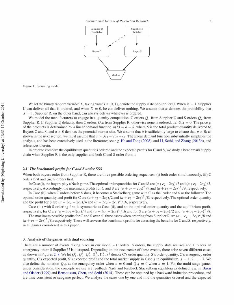
To investigate the impact of supply disruptions on competing buyers, we consider a supply chain as depicted in Figure 1.There are two Buyers, C and S, who procure parts from Suppliers U and R. Buyers C and S process these parts into substitutableproducts to be sold at the same price in the market to end consumers. The product has a short life cycle and is sold in asingle-selling season. Supplier U is unreliable and Supplier R is reliable, and the unit costs charged by them are c1 and c2,respectively, where c2 > c1 > 0 for regular orders. In normal situations (without supply disruptions), C buys products fromSupplier U. If Supplier U defaults, C places an emergency order with Supplier R at a unit cost of c3 where c3 ≥ c2 on accountof S being Supplier R’s preferred customer. We should note here that an issue of whether the scenario we model in thissection could arise endogenously could be raised. To answer this, we provide in Section 6.1 an example of two asymmetricfirms C and S with c3 > c2 in which Firm C chooses CDSS and Firm S chooses SSS when the reliability of Supplier U is ata medium level. Of course, here we study the case in the general parameter settings of c3 ≥ c2 and α ∈ [0, 1].

Dow

nloa

ded

by [

Nip

issi

ng U

nive

rsity

] at

13:

31 1

7 O

ctob

er 2

014

International Journal of Production Research 3

Figure 1. Sourcing model.

We let the binary random variable X , taking values in {0, 1}, denote the supply state of Supplier U. When X = 1, SupplierU can deliver all that is ordered, and when X = 0, he can deliver nothing. We assume that α denotes the probability thatX = 1. Supplier R, on the other hand, can always deliver whatever is ordered.

We model the manufacturers to engage in a quantity competition. C orders Q1 from Supplier U and S orders Q2 fromSupplier R. If Supplier U defaults, then C orders Qe0 from Supplier R, otherwise none is ordered, i.e. Qe1 = 0. The price pof the products is determined by a linear demand function p(S) = a − S, where S is the total product quantity delivered toBuyers C and S, and a > 0 denotes the potential market size. We assume that a is sufficiently large to ensure that p > 0; asshown in the next section, we must assume that a > 3c3 − 2c2 + c1. The linear demand function substantially simplifies theanalysis, and has been extensively used in the literature; see e.g. Ha and Tong (2008), and Li, Sethi, and Zhang (2013b), andreferences therein.

In order to compare the equilibrium quantities ordered and the expected profits for C and S, we study a benchmark supplychain when Supplier R is the only supplier and both C and S order from it.

2.1 The benchmark profits for C and S under SSS

When both buyers order from Supplier R, there are three possible ordering sequences: (i) both order simultaneously, (ii) Corders first and (iii) S orders first.

In Case (i), the buyers play a Nash game. The optimal order quantities for C and S are (a+c2−2c3)/3 and (a+c3−2c2)/3,respectively. Accordingly, the maximum profits for C and S are (a + c2 − 2c3)

2 /9 and (a + c3 − 2c2)2 /9, respectively.

In Case (ii), when C orders before S does, it becomes a Stackelberg game with C as the leader and S as the follower. Theoptimal order quantity and profit for C are (a + c2 − 2c3)/2 and (a + c2 − 2c3)

2 /8, respectively. The optimal order quantityand the profit for S are (a − 3c2 + 2c3)/4 and (a − 3c2 + 2c3)

2 /16, respectively.Case (iii) with S ordering first is symmetric to Case (ii), and so the optimal order quantity and the equilibrium profit,

respectively, for C are (a − 3c3 + 2c2)/4 and (a − 3c3 + 2c2)2 /16 and for S are (a + c3 − 2c2)/2 and (a + c3 − 2c2)

2 /8.The maximum possible profits for C and S over all three cases when ordering from Supplier R are (a + c2 − 2c3)

2 /8 and(a + c3 − 2c2)

2 /8, respectively. These will serve as the benchmark profits for assessing the benefits for C and S, respectively,in all games considered in this paper.

3. Analysis of the games with dual sourcing

There are a number of events taking place in our model – C orders, S orders, the supply state realizes and C places anemergency order if Supplier U is disrupted. Depending on the occurrence of these events, there arise seven different casesas shown in Figures 2–8. We let Q j

1, Q j2, Q j

e ,�jC,�

jS, S j denote C’s order quantity, S’s order quantity, C’s emergency order

quantity, C’s expected profit, S’s expected profit and the total market supply in Case j in equilibrium, j = 1, 2, . . . , 7. Wealso define the notation Qe0 as the emergency order when x = 0 and Qe1 = 0 when x = 1. For the multi-stage gamesunder consideration, the concepts we use are feedback Nash and feedback Stackelberg equilibria as defined, e.g. in Basarand Olsder (1999) and Bensoussan, Chen, and Sethi (2014). These can be obtained by a backward induction procedure, andare time consistent or subgame perfect. We analyse the cases one by one and find the quantities ordered and the expected

Dow

nloa

ded

by [

Nip

issi

ng U

nive

rsity

] at

13:

31 1

7 O

ctob

er 2

014

4 V. Gupta et al.

Figure 2. Sequence of events for Case 1.

profits in equilibrium in each case. We also discuss the sensitivity of the results with respect to the model parameters ineach case. We obtain managerial insights indicating how the results change with respect to the model parameters in eachcase.

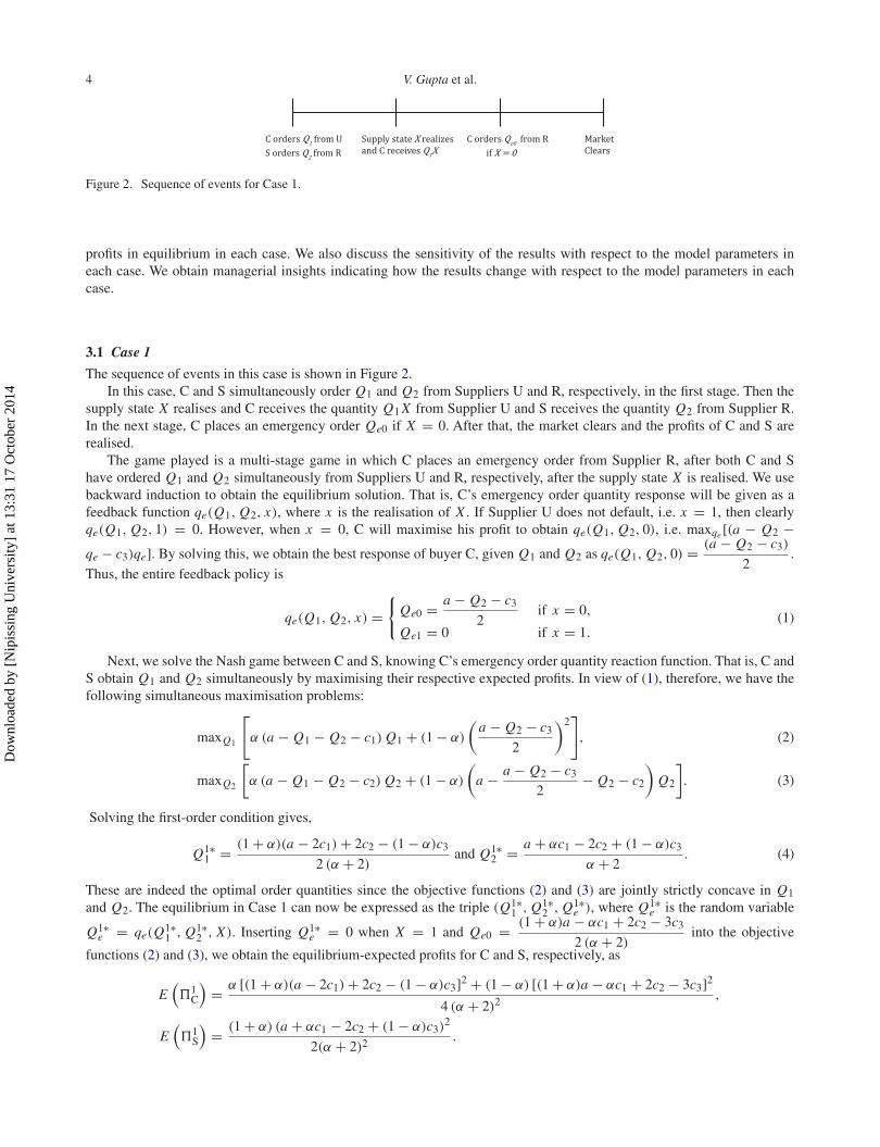
3.1 Case 1

The sequence of events in this case is shown in Figure 2.In this case, C and S simultaneously order Q1 and Q2 from Suppliers U and R, respectively, in the first stage. Then the

supply state X realises and C receives the quantity Q1 X from Supplier U and S receives the quantity Q2 from Supplier R.In the next stage, C places an emergency order Qe0 if X = 0. After that, the market clears and the profits of C and S arerealised.

The game played is a multi-stage game in which C places an emergency order from Supplier R, after both C and Shave ordered Q1 and Q2 simultaneously from Suppliers U and R, respectively, after the supply state X is realised. We usebackward induction to obtain the equilibrium solution. That is, C’s emergency order quantity response will be given as afeedback function qe(Q1, Q2, x), where x is the realisation of X . If Supplier U does not default, i.e. x = 1, then clearlyqe(Q1, Q2, 1) = 0. However, when x = 0, C will maximise his profit to obtain qe(Q1, Q2, 0), i.e. maxqe [(a − Q2 −qe − c3)qe]. By solving this, we obtain the best response of buyer C, given Q1 and Q2 as qe(Q1, Q2, 0) = (a − Q2 − c3)

2.

Thus, the entire feedback policy is

qe(Q1, Q2, x) ={

Qe0 = a − Q2 − c3

2if x = 0,

Qe1 = 0 if x = 1.(1)

Next, we solve the Nash game between C and S, knowing C’s emergency order quantity reaction function. That is, C andS obtain Q1 and Q2 simultaneously by maximising their respective expected profits. In view of (1), therefore, we have thefollowing simultaneous maximisation problems:

maxQ1

[α (a − Q1 − Q2 − c1) Q1 + (1 − α)

(a − Q2 − c3

2

)2], (2)

maxQ2

[α (a − Q1 − Q2 − c2) Q2 + (1 − α)

(a − a − Q2 − c3

2− Q2 − c2

)Q2

]. (3)

Solving the first-order condition gives,

Q1∗1 = (1 + α)(a − 2c1) + 2c2 − (1 − α)c3

2 (α + 2)and Q1∗

2 = a + αc1 − 2c2 + (1 − α)c3

α + 2. (4)

These are indeed the optimal order quantities since the objective functions (2) and (3) are jointly strictly concave in Q1and Q2. The equilibrium in Case 1 can now be expressed as the triple (Q1∗

1 , Q1∗2 , Q1∗

e ), where Q1∗e is the random variable

Q1∗e = qe(Q1∗

1 , Q1∗2 , X). Inserting Q1∗

e = 0 when X = 1 and Qe0 = (1 + α)a − αc1 + 2c2 − 3c3

2 (α + 2)into the objective

functions (2) and (3), we obtain the equilibrium-expected profits for C and S, respectively, as

E(�1

C

)= α [(1 + α)(a − 2c1) + 2c2 − (1 − α)c3]2 + (1 − α) [(1 + α)a − αc1 + 2c2 − 3c3]2

4 (α + 2)2,

E(�1

S

)= (1 + α) (a + αc1 − 2c2 + (1 − α)c3)

2

2(α + 2)2.

Dow

nloa

ded

by [

Nip

issi

ng U

nive

rsity

] at

13:

31 1

7 O

ctob

er 2

014

International Journal of Production Research 5

The expected total market output is

E(

S1)

= α(

Q1∗1 + Q1∗

2

)+ (1 − α)

(Q1∗

e + Q1∗2

)= (3 + α)a − α(1 + α)c1 − 2c2 − (1 − α2)c3

2 (α + 2).

Proposition 1 Q1∗1 increases in α and c2 and decreases in c1 and c3; Q1∗

2 decreases in α and c2 and increases in c1 andc3; and Q1∗

e increases in α and decreases in c1, c2 and c3, almost surely.

Proposition 1 says that when c2 increases, Supplier U has a higher cost advantage over supplier R. So, C increases thequantity ordered from supplier U. When c1 increases, the cost advantage for C reduces and he buys less from supplier U. Anincrease in supplier U’s reliability α means that C has a higher chance of realising the cost advantage over S, and therefore,C buys more and S buys less from Supplier R.

Proposition 2 In the equilibrium in Case 1, the expected total market output decreases in c1, c2 and c3, and increases inα if 2c2 + (

α2 + 4α + 1)

c3 > a + (α2 + 4α + 2

)c1 and does not increase otherwise.

The expected market price in Case 1 is E(

p1) = a − E

(S1

), and it is straightforward to obtain the results about the

expected market price from the expected total market supply.

3.2 Case 2

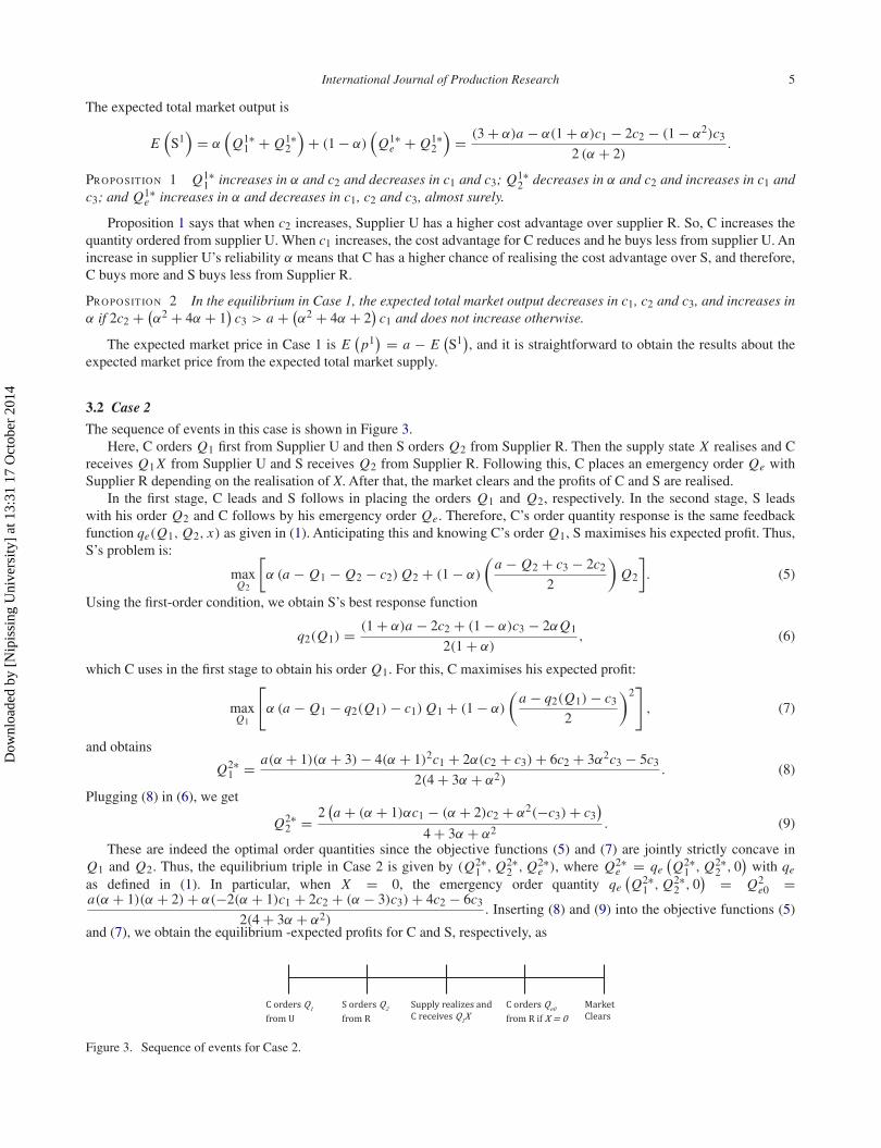
The sequence of events in this case is shown in Figure 3.Here, C orders Q1 first from Supplier U and then S orders Q2 from Supplier R. Then the supply state X realises and C

receives Q1 X from Supplier U and S receives Q2 from Supplier R. Following this, C places an emergency order Qe withSupplier R depending on the realisation of X. After that, the market clears and the profits of C and S are realised.

In the first stage, C leads and S follows in placing the orders Q1 and Q2, respectively. In the second stage, S leadswith his order Q2 and C follows by his emergency order Qe. Therefore, C’s order quantity response is the same feedbackfunction qe(Q1, Q2, x) as given in (1). Anticipating this and knowing C’s order Q1, S maximises his expected profit. Thus,S’s problem is:

maxQ2

[α (a − Q1 − Q2 − c2) Q2 + (1 − α)

(a − Q2 + c3 − 2c2

2

)Q2

]. (5)

Using the first-order condition, we obtain S’s best response function

q2(Q1) = (1 + α)a − 2c2 + (1 − α)c3 − 2αQ1

2(1 + α), (6)

which C uses in the first stage to obtain his order Q1. For this, C maximises his expected profit:

maxQ1

[α (a − Q1 − q2(Q1) − c1) Q1 + (1 − α)

(a − q2(Q1) − c3

2

)2]

, (7)

and obtains

Q2∗1 = a(α + 1)(α + 3) − 4(α + 1)2c1 + 2α(c2 + c3) + 6c2 + 3α2c3 − 5c3

2(4 + 3α + α2). (8)

Plugging (8) in (6), we get

Q2∗2 = 2

(a + (α + 1)αc1 − (α + 2)c2 + α2(−c3) + c3

)4 + 3α + α2

. (9)

These are indeed the optimal order quantities since the objective functions (5) and (7) are jointly strictly concave inQ1 and Q2. Thus, the equilibrium triple in Case 2 is given by (Q2∗

1 , Q2∗2 , Q2∗

e ), where Q2∗e = qe

(Q2∗

1 , Q2∗2 , 0

)with qe

as defined in (1). In particular, when X = 0, the emergency order quantity qe(Q2∗

1 , Q2∗2 , 0

) = Q2e0 =

a(α + 1)(α + 2) + α(−2(α + 1)c1 + 2c2 + (α − 3)c3) + 4c2 − 6c3

2(4 + 3α + α2). Inserting (8) and (9) into the objective functions (5)

and (7), we obtain the equilibrium -expected profits for C and S, respectively, as

Figure 3. Sequence of events for Case 2.

Dow

nloa

ded

by [

Nip

issi

ng U

nive

rsity

] at

13:

31 1

7 O

ctob

er 2

014

6 V. Gupta et al.

E(�2

C

)= 1

4(4 + 3α + α2)

[α2(a2 + a(6c3 − 8c1) + 8c2

1 − 4c1(c2 + c3) + c3(4c2 − 3c3))

+2α(a2 − a(3c1 − 2c2 + c3) + 2c2

1 + c1(5c3 − 6c2) + 4c3(c2 − c3))

+2α3(c3 − c1)(a − 2c1 + c3) + (a + 2c2 − 3c3)2],

E(�2

S

)= 2(α + 1)

(a + (α + 1)αc1 − (α + 2)c2 + α2(−c3) + c3

)2

(4 + 3α + α2)2.

The expected total market output E(S2

)is given by

E(

S2)

= Q2∗2 + αQ2∗

1 + (1 − α) Q2∗e0 = a(α(α + 2) + 3) + (α + 1)2((α − 1)c3 − αc1) − 2c2

4 + 3α + α2.

Proposition 3 The expected total market supply E(S2

)decreases in c1, c2 and c3, and increases in α if

6c2 − c3 + a(−1 + α(2 + α)) − c1(1 + α)(4 + α(12 + α(5 + α))) + α(4c2 + c3(10 + α(16 + α(6 + α)))) > 0.

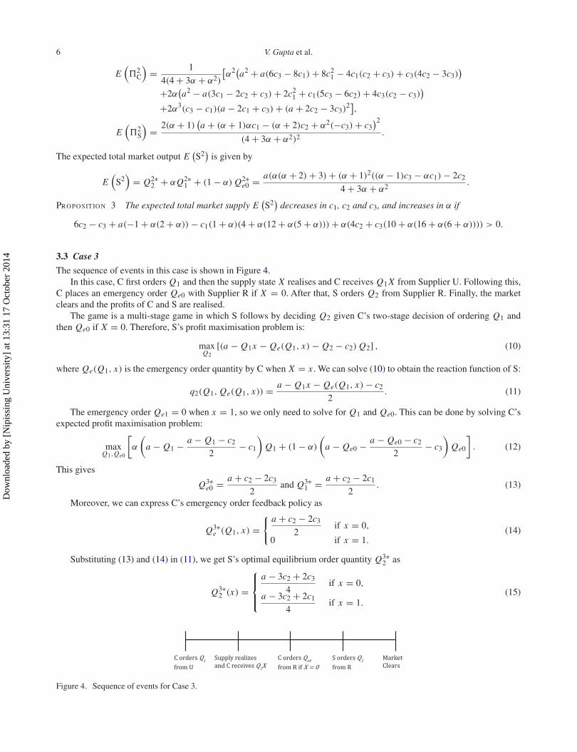
3.3 Case 3

The sequence of events in this case is shown in Figure 4.In this case, C first orders Q1 and then the supply state X realises and C receives Q1 X from Supplier U. Following this,

C places an emergency order Qe0 with Supplier R if X = 0. After that, S orders Q2 from Supplier R. Finally, the marketclears and the profits of C and S are realised.

The game is a multi-stage game in which S follows by deciding Q2 given C’s two-stage decision of ordering Q1 andthen Qe0 if X = 0. Therefore, S’s profit maximisation problem is:

maxQ2

[(a − Q1x − Qe(Q1, x) − Q2 − c2) Q2] , (10)

where Qe(Q1, x) is the emergency order quantity by C when X = x . We can solve (10) to obtain the reaction function of S:

q2(Q1, Qe(Q1, x)) = a − Q1x − Qe(Q1, x) − c2

2. (11)

The emergency order Qe1 = 0 when x = 1, so we only need to solve for Q1 and Qe0. This can be done by solving C’sexpected profit maximisation problem:

maxQ1,Qe0

[α

(a − Q1 − a − Q1 − c2

2− c1

)Q1 + (1 − α)

(a − Qe0 − a − Qe0 − c2

2− c3

)Qe0

]. (12)

This gives

Q3∗e0 = a + c2 − 2c3

2and Q3∗

1 = a + c2 − 2c1

2. (13)

Moreover, we can express C’s emergency order feedback policy as

Q3∗e (Q1, x) =

{ a + c2 − 2c3

2if x = 0,

0 if x = 1.(14)

Substituting (13) and (14) in (11), we get S’s optimal equilibrium order quantity Q3∗2 as

Q3∗2 (x) =

⎧⎪⎨⎪⎩

a − 3c2 + 2c3

4if x = 0,

a − 3c2 + 2c1

4if x = 1.

(15)

Figure 4. Sequence of events for Case 3.

Dow

nloa

ded

by [

Nip

issi

ng U

nive

rsity

] at

13:

31 1

7 O

ctob

er 2

014

International Journal of Production Research 7

Inserting (13)–(15) into the objective functions (10) and (12), we obtain the equilibrium-expected profits for C and S as

E(�3

C

)= α

(a + c2 − 2c1)2

8+ (1 − α)

(a + c2 − 2c3)2

8,

E(�3

S

)= α

(a − 3c2 + 2c1)2

16+ (1 − α)

(a − 3c2 + 2c3)

16

2

.

It is easy to see that E(�3

C

)> E

(�3

S

)when c2 = c3. Also, E

(�3

C

)< E

(�3

S

)for large values of c3 and small α. The

expected total market output is

E(

S3)

= α

(a + c2 − 2c1

2+ a − 3c2 + 2c1

4

)+ (1 − α)

(a + c2 − 2c3

2+ a − 3c2 + 2c3

4

)

= 3a − 2αc1 − c2 − 2(1 − α)c3

4.

Proposition 4 At the equilibrium of Case 3, the expected total market output E(S3

)increases in α and decreases in c1,

c2 and c3. The expected market price E(

p4)

decreases in α and increases in c1, c2 and c3.

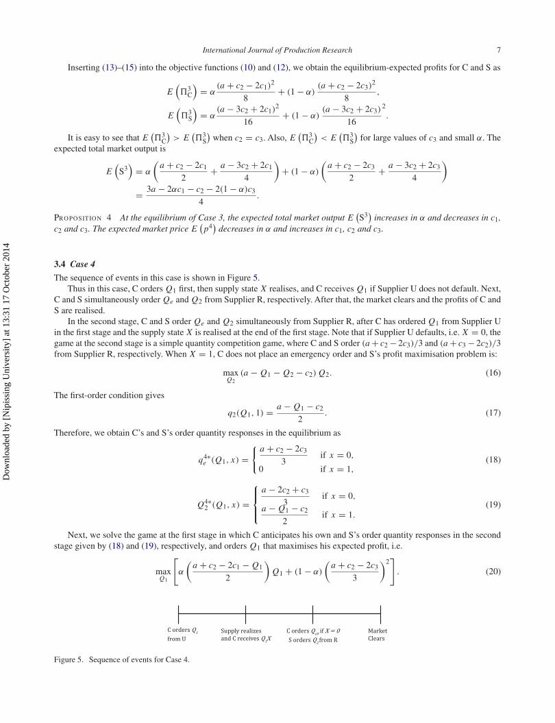
3.4 Case 4

The sequence of events in this case is shown in Figure 5.Thus in this case, C orders Q1 first, then supply state X realises, and C receives Q1 if Supplier U does not default. Next,

C and S simultaneously order Qe and Q2 from Supplier R, respectively. After that, the market clears and the profits of C andS are realised.

In the second stage, C and S order Qe and Q2 simultaneously from Supplier R, after C has ordered Q1 from Supplier Uin the first stage and the supply state X is realised at the end of the first stage. Note that if Supplier U defaults, i.e. X = 0, thegame at the second stage is a simple quantity competition game, where C and S order (a + c2 − 2c3)/3 and (a + c3 − 2c2)/3from Supplier R, respectively. When X = 1, C does not place an emergency order and S’s profit maximisation problem is:

maxQ2

(a − Q1 − Q2 − c2) Q2. (16)

The first-order condition gives

q2(Q1, 1) = a − Q1 − c2

2. (17)

Therefore, we obtain C’s and S’s order quantity responses in the equilibrium as

q4∗e (Q1, x) =

{ a + c2 − 2c3

3if x = 0,

0 if x = 1,(18)

Q4∗2 (Q1, x) =

⎧⎪⎨⎪⎩

a − 2c2 + c3

3if x = 0,

a − Q1 − c2

2if x = 1.

(19)

Next, we solve the game at the first stage in which C anticipates his own and S’s order quantity responses in the secondstage given by (18) and (19), respectively, and orders Q1 that maximises his expected profit, i.e.

maxQ1

[α

(a + c2 − 2c1 − Q1

2

)Q1 + (1 − α)

(a + c2 − 2c3

3

)2]

. (20)

Figure 5. Sequence of events for Case 4.

Dow

nloa

ded

by [

Nip

issi

ng U

nive

rsity

] at

13:

31 1

7 O

ctob

er 2

014

8 V. Gupta et al.

From the first-order condition, we solve for Q4∗1 , C’s optimal order quantity in stage 1, as

Q4∗1 = a + c2 − 2c1

2. (21)

Substituting (21) into (19), we have Q4∗2 = a − 3c2 + 2c1

4, if x = 1. Using the equilibrium order quantities, we can now

derive the expected profits for C and S as

E(�4

C

)= α

(a + c2 − 2c1)2

8+ (1 − α)

(a + c2 − 2c3)2

9,

E(�4

S

)= α

(a − 3c2 + 2c1)2

16+ (1 − α)

(a − 2c2 + c3)2

9.

It is easy to see that E(�4

C

)> E

(�4

S

)when c2 = c3. Also, E

(�4

C

)< E

(�4

S

)for large values of c3 and small α. The

expected total market output is

E(

S4)

= α

(a + c2 − 2c1

2+ a − 3c2 + 2c1

4

)+ (1 − α)

(a + c2 − 2c3

3+ a − 2c2 + c3

3

),

= α

(3a − c2 − 2c1

4

)+ (1 − α)

(2a − c2 − c3

3

).

Proposition 5 In the equilibrium of Case 4, the expected total market output E(S4

)increases in α and decreases in c1,

c2 and c3. Consequently, the expected market price E(

p4)

decreases in α but increases in c1, c2 and c3.

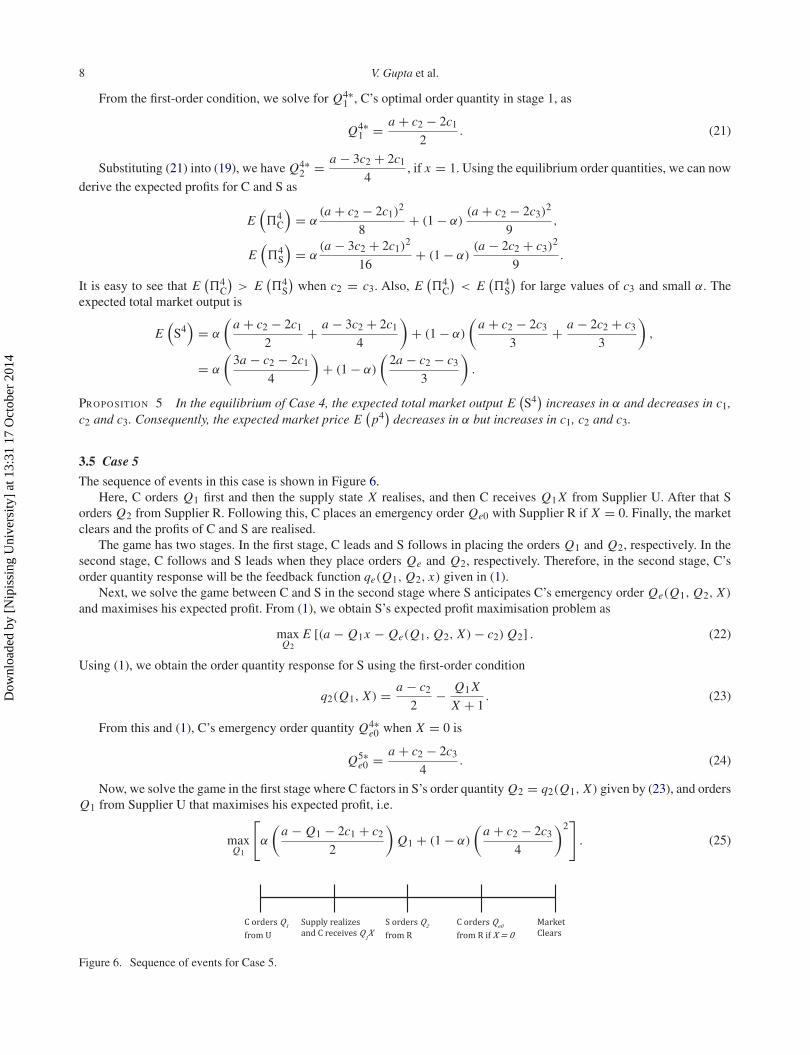
3.5 Case 5

The sequence of events in this case is shown in Figure 6.Here, C orders Q1 first and then the supply state X realises, and then C receives Q1 X from Supplier U. After that S

orders Q2 from Supplier R. Following this, C places an emergency order Qe0 with Supplier R if X = 0. Finally, the marketclears and the profits of C and S are realised.

The game has two stages. In the first stage, C leads and S follows in placing the orders Q1 and Q2, respectively. In thesecond stage, C follows and S leads when they place orders Qe and Q2, respectively. Therefore, in the second stage, C’sorder quantity response will be the feedback function qe(Q1, Q2, x) given in (1).

Next, we solve the game between C and S in the second stage where S anticipates C’s emergency order Qe(Q1, Q2, X)

and maximises his expected profit. From (1), we obtain S’s expected profit maximisation problem as

maxQ2

E [(a − Q1x − Qe(Q1, Q2, X) − c2) Q2] . (22)

Using (1), we obtain the order quantity response for S using the first-order condition

q2(Q1, X) = a − c2

2− Q1 X

X + 1. (23)

From this and (1), C’s emergency order quantity Q4∗e0 when X = 0 is

Q5∗e0 = a + c2 − 2c3

4. (24)

Now, we solve the game in the first stage where C factors in S’s order quantity Q2 = q2(Q1, X) given by (23), and ordersQ1 from Supplier U that maximises his expected profit, i.e.

maxQ1

[α

(a − Q1 − 2c1 + c2

2

)Q1 + (1 − α)

(a + c2 − 2c3

4

)2]

. (25)

Figure 6. Sequence of events for Case 5.

Dow

nloa

ded

by [

Nip

issi

ng U

nive

rsity

] at

13:

31 1

7 O

ctob

er 2

014

International Journal of Production Research 9

Solving this, gives

Q5∗1 = a + c2 − 2c1

2. (26)

Plugging (26) in (23), we obtain

Q5∗2 (x) =

⎧⎪⎨⎪⎩

a − c2

2if x = 0,

a − 3c2 + 2c1

4if x = 1.

(27)

The expected profits for C and S are

E(�5

C

)= α

(a + c2 − 2c1)2

8+ (1 − α)

(a + c2 − 2c3)2

16,

E(�5

S

)= α

(a − 3c2 + 2c1)2

16+ (1 − α)

(a − c2)2

8.

The expected total market output is

E(

S5)

= α

(a + c2 − 2c1

2+ a − 3c2 + 2c1

4

)+ (1 − α)

(a + c2 − 2c3

4+ a − c2

2

)

= α

(3a − c2 − 2c1

4

)+ (1 − α)

(3a − c2 − 2c3

4

)

= 3a − 2αc1 − c2 − 2(1 − α)c3

4.

Proposition 6 In the equilibrium, E(S5

)increases in α and decreases in c1, c2, and c3. The expected market price E

(p5

)decreases in α and increases in c1, c2, and c3.

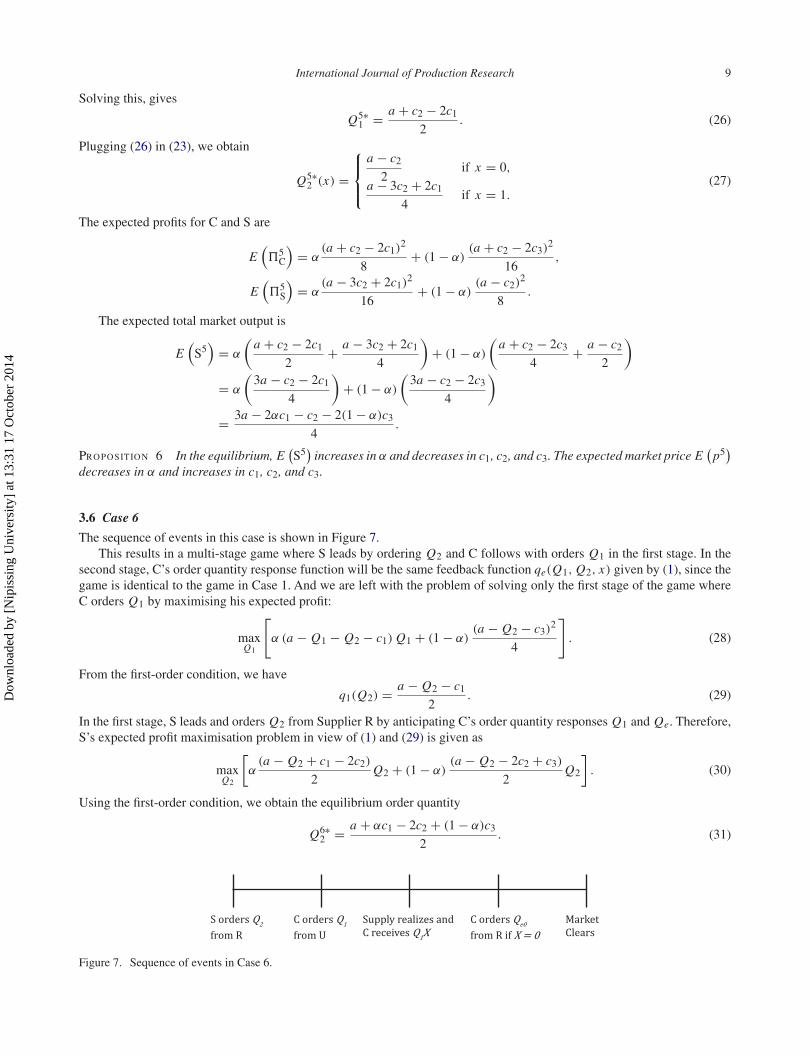
3.6 Case 6

The sequence of events in this case is shown in Figure 7.This results in a multi-stage game where S leads by ordering Q2 and C follows with orders Q1 in the first stage. In the

second stage, C’s order quantity response function will be the same feedback function qe(Q1, Q2, x) given by (1), since thegame is identical to the game in Case 1. And we are left with the problem of solving only the first stage of the game whereC orders Q1 by maximising his expected profit:

maxQ1

[α (a − Q1 − Q2 − c1) Q1 + (1 − α)

(a − Q2 − c3)2

4

]. (28)

From the first-order condition, we have

q1(Q2) = a − Q2 − c1

2. (29)

In the first stage, S leads and orders Q2 from Supplier R by anticipating C’s order quantity responses Q1 and Qe. Therefore,S’s expected profit maximisation problem in view of (1) and (29) is given as

maxQ2

[α

(a − Q2 + c1 − 2c2)

2Q2 + (1 − α)

(a − Q2 − 2c2 + c3)

2Q2

]. (30)

Using the first-order condition, we obtain the equilibrium order quantity

Q6∗2 = a + αc1 − 2c2 + (1 − α)c3

2. (31)

Figure 7. Sequence of events in Case 6.

Dow

nloa

ded

by [

Nip

issi

ng U

nive

rsity

] at

13:

31 1

7 O

ctob

er 2

014

10 V. Gupta et al.

From (1), (29), and (31), we obtain

Q6∗1 = a − (2 + α)c1 + 2c2 − (1 − α)c3

4, (32)

q6∗e (x) =

{ a − αc1 + 2c2 − (3 − α)c3

4if x = 0,

0 if x = 1.(33)

Using these order quantities, we find the expected profits for C and S as

E(�6

C

)= α

(a − (α + 2)c1 + 2c2 − (1 − α)c3

4

)2

+ (1 − α)

(a − αc1 + 2c2 − (3 − α)c3

4

)2

= 1

16

((a + 2c2 − 3c3)

2 + 2(3a − 2c1 + 6c2 − 7c3)(−c1 + c3)α + 5(c1 − c3)2α2

),

E(�6

S

)=

{α

(a − 3c2 + αc2 − αc1 + 2c1

4

)+ (1 − α)

(a − c2 + αc2 − αc1

4

)} (a − c2 − αc2 + αc1

2

)

= 1

8(a + αc1 − 2c2 + (1 − α)c3)

2.

Here, a direct comparison of C’s and S’s expected profit is not straightforward. So, we resort to numerical analysis in Section5 to compare the profits. The expected total market output is

E(

S6)

= α

(a − (2 + α)c1 + 2c2 − (1 − α)c3

4+ a + αc1 − 2c2 + (1 − α)c3

2

)

+ (1 − α)

(a − αc1 + 2c2 − (3 − α)c3

4+ a + αc1 − 2c2 + (1 − α)c3

2

)

= 1

4(3a − αc1 − 2c2 − (1 − α)c3) .

Proposition 7 In the equilibrium of Case 6, the E(S6

)increases in α and decreases in c1, c2, and c3. p6 decreases in α

and increases in c1, c2, and c3.

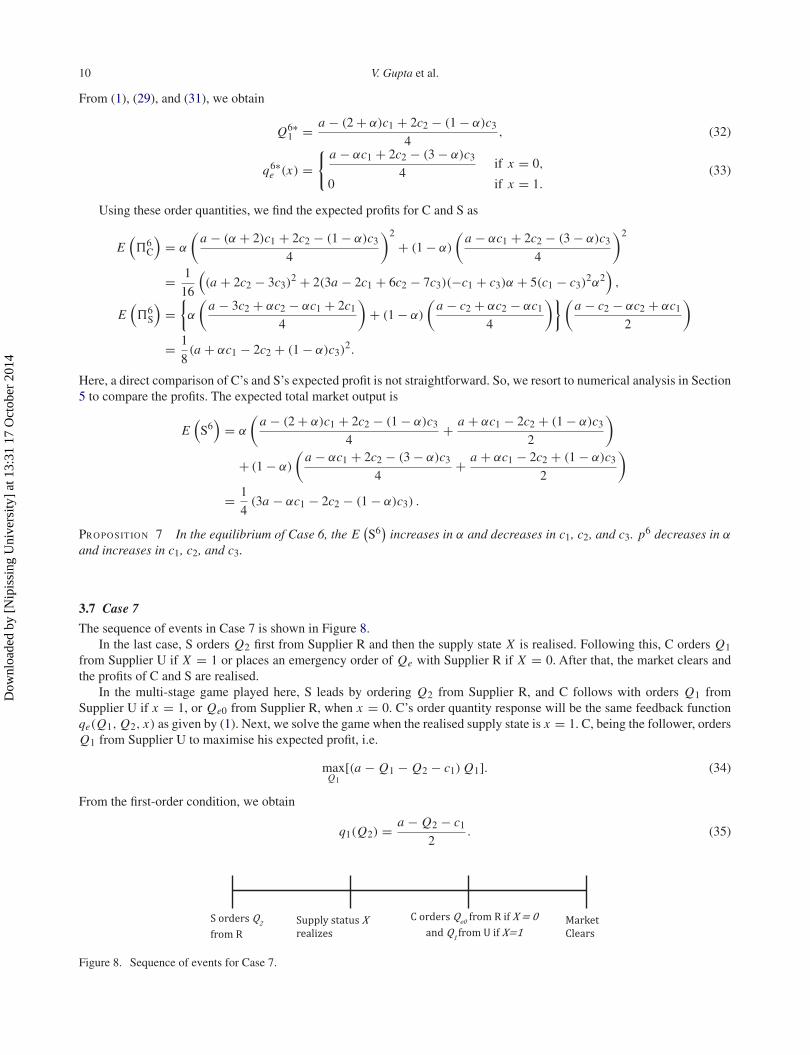
3.7 Case 7

The sequence of events in Case 7 is shown in Figure 8.In the last case, S orders Q2 first from Supplier R and then the supply state X is realised. Following this, C orders Q1

from Supplier U if X = 1 or places an emergency order of Qe with Supplier R if X = 0. After that, the market clears andthe profits of C and S are realised.

In the multi-stage game played here, S leads by ordering Q2 from Supplier R, and C follows with orders Q1 fromSupplier U if x = 1, or Qe0 from Supplier R, when x = 0. C’s order quantity response will be the same feedback functionqe(Q1, Q2, x) as given by (1). Next, we solve the game when the realised supply state is x = 1. C, being the follower, ordersQ1 from Supplier U to maximise his expected profit, i.e.

maxQ1

[(a − Q1 − Q2 − c1) Q1]. (34)

From the first-order condition, we obtain

q1(Q2) = a − Q2 − c1

2. (35)

Figure 8. Sequence of events for Case 7.

Dow

nloa

ded

by [

Nip

issi

ng U

nive

rsity

] at

13:

31 1

7 O

ctob

er 2

014

International Journal of Production Research 11

S anticipates C’s order quantities (1) and (35), and orders Q2 from Supplier R that maximises his expected profit:

maxQ2

[α

(a − Q2 + c1 − 2c2)

2Q2 + (1 − α)

(a − Q2 − 2c2 + c3)

2Q2

]. (36)

The first-order condition gives S’s equilibrium order quantity Q7∗2 for the first-stage game as

Q7∗2 = a − 2c2 + αc1 + (1 − α)c3

2. (37)

From (1), (35), and (37), we obtain the equilibrium order quantities Q7∗1 = a − (2 + α)c1 + 2c2 − (1 − α)c3

4and

Q7∗e = a − αc1 + 2c2 − (3 − α)c3

4. The expected profits of C and S are

E(�7

C

)= α

(a − (α + 2)c1 + 2c2 − (1 − α)c3

4

)2

+ (1 − α)

(a − αc1 + 2c2 − (3 − α)c3

4

)2

= 1

16

((a + 2c2 − 3c3)

2 + 2(3a − 2c1 + 6c2 − 7c3)(−c1 + c3)α + 5(c1 − c3)2α2

),

E(�7

S

)=

{α

(a − 3c2 + αc2 − αc1 + 2c1

4

)+ (1 − α)

(a − c2 + αc2 − αc1

4

)} (a − c2 − αc2 + αc1

2

)

= 1

8(a + αc1 − 2c2 + (1 − α)c3)

2.

The expected total market output is identical to that in Case 6. Since E(S7

) = E(S6

), all other equilibrium results in Case

7 are identical to those in Case 6.

4. Equilibrium profit comparisons

In the previous section, we derived explicit expressions for the Equilibrium-expected profits of C and S in all cases. In Section2.1, we obtained the benchmark profit. In this section, we compare the expected profits of C and S in all seven cases and alsoto the benchmark profit.

Proposition 8 (i) Expected profits for C satisfy: E(�2

C

)> E

(�1

C

)> E

(�6

C

) = E(�7

C

), E

(�3

C

)> E

(�4

C

)>

E(�5

C

), and E

(�5

C

)> E

(�1

C

).

(ii) Expected profits for S satisfy: E(�2

S

)< E

(�1

S

)< E

(�6

S

) = E(�7

S

), E

(�3

S

)< E

(�4

S

)< E

(�5

S

), and

E(�1

S

)> E

(�4

S

).

(iii) The expected profits of C satisfy E(�iC) ≤ �0

C for i �= 3 and E(�3C) > �0

C = (a + c2 − 2c3)2/8, the benchmark

profit. The expected profits of S in all cases satisfy E(�iS) ≤ �0

C. Finally, E(�3

C

)> E

(�3

S

).

As we go from Case 3 to Case 5, we see from Propositions 8 (i) and (ii) that the time when S places orders. This confersan advantage to S, and consequently his expected profit increases and the expected profit of C decreases.

In Proposition 8(iii), we compare the expected profits of C with the benchmark profit �0C. We observe that only in

Case 3, C has a higher profit than its benchmark profit. The intuitive explanation is that purchasing from an unreliablesupplier is better for someone with first-mover advantage and when the supply state is realised before the competitor orders.Similarly, the equilibrium-expected profits of S are less than the benchmark profit in all cases. Therefore, the profit of C isalways more than the profit of S in Case 3. This is further corroborated by the numerical computations in Section 5.

Proposition 9 If α ≥ 0.5 and c2 = c3, then E(�5

C

)> E

(�5

S

).

4.1 Comparative statics

The comparative statics of the equilibrium-expected profits of C and S are summarised in Table 1. We see that the equilibrium-expected profits for both C and S are monotone in α, c1 and c3. C’s profit is not monotone with c2, and S’s profit is decreasingwith c2. In the absence of monotonicity of E(�i

C) with c2, we conjecture that when the supply from 1 is highly reliable,E(�i

C) increases in c2, and when the supply from 1 is highly unreliable, E(�iC) decreases in c2. The intuitive explanation

for this conjecture relies on the trade-off between the supply costs c1, c2 and c3 to C and S and the reliability α of Supplier U.With a higher reliability of Supplier U, the chance of order fulfilment is higher, i.e. C purchases at the cheaper price c1 fromSupplier U with a higher chance. Subsequently, C earns more in the market due to his cost advantage over S since c2 ≥ c1.

Dow

nloa

ded

by [

Nip

issi

ng U

nive

rsity

] at

13:

31 1

7 O

ctob

er 2

014

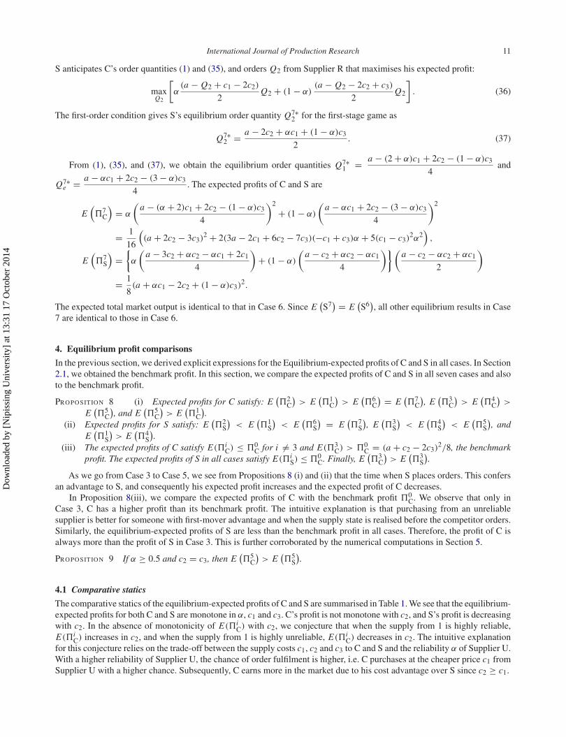
12 V. Gupta et al.

Table 1. Comparative statics of Equilibrium-expected profits under cases i = 1, . . . , 7. Here, ‘↑’ indicates increasing, ‘↓’ indicatesdecreasing and ‘’ indicates non-monotonicity.

∂ E(�i

C

)∂α

∂ E(�i

C

)∂c1, c3

∂ E(�i

C

)∂c2

∂ E(�i

S

)∂α

∂ E(�i

S

)∂c1, c3

∂ E(�i

S

)∂c2

↑ ↓ ↓ ↑ ↓

Table 2. Comparative statics of equilibrium order quantities. Here, ↑ indicates increasing, ↓ indicates decreasing, and indicatesunchanging. ↑ () and ↓ () indicates increasing and decreasing in c1, respectively, and unchanging in c3. (↓) indicates unchanging inc1 and decreasing in c3.

Order quantity → Qi∗1 Qi∗

2 Qi∗e0

Parameter → α c1(c3) c2 α c1(c3) c2 α c1(c3) c2

Case 1 ↑ ↓ ↑ ↓ ↑ ↓ ↑ ↓ ↑Case 2 ↑ ↓ ↑ ↓ ↑ ↓ ↑ ↓ ↑Case 3 ↓ () ↑ ↓ ↑ ↓ (↓) ↑Case 4 ↓ () ↑ ↑ ↓ (↓) ↑Case 5 ↓ () ↑ ↑ ↑ () ↓ (↓) ↑Case 6 ↓ ↓ ↑ ↑ ↑ ↓ ↓ ↓ ↑Case 7 ↓ ↓ ↑ ↑ ↑ ↓ ↓ ↓ ↑

We now summarise the comparative statics of the equilibrium order quantities for C and S in all seven cases. The mostinteresting takeaway from Table 2 is the impact of reliability on the order quantities. We see that Qi∗

1 and Qi∗e0 are increasing

in α in Cases 1 and 2, where C orders from Supplier U before or at the same time as S does from Supplier R. In Cases6 and 7, S orders from Supplier R before C does from Suppliers U and R. Therefore, both Qi∗

1 and Qi∗e0 are decreasing in

α in Cases 6 and 7. Similarly, we see that Qi∗2 is decreasing in α in Cases 1 and 2 and increasing in α for Cases 6 and 7,

respectively. We also see from Table 2 that the quantity ordered by a firm is always non-increasing in its own procurementcosts and non-decreasing in its competitor’s procurement costs.

5. Computational analysis

In this section, we present the results obtained from computations that confirm as well as add to the conclusions drawn inSection 3. We compute the expected equilibrium profits for both C and S in all cases by varying c1, c2, c3 and α. Since theequilibrium profits of C as well as S are identical in Cases 6 and 7, we analyse them together as ‘cases 6, 7’. The profits of Cand S are monotone in the same direction with both c1 and c3, so we assume c3 = c2 when analysing the impacts of c1 andc2 on the equilibrium-expected profits of C and S. In particular, we first illustrate the impact of combinations of α, c1 and c2on the equilibrium-expected profits of C and S and on the equilibrium total order quantities in all cases. We let a = 100 inall computations.

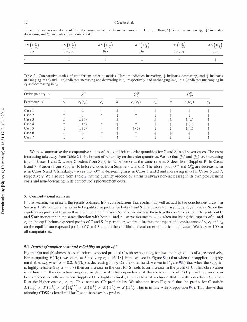
5.1 Impact of supplier costs and reliability on profit of C

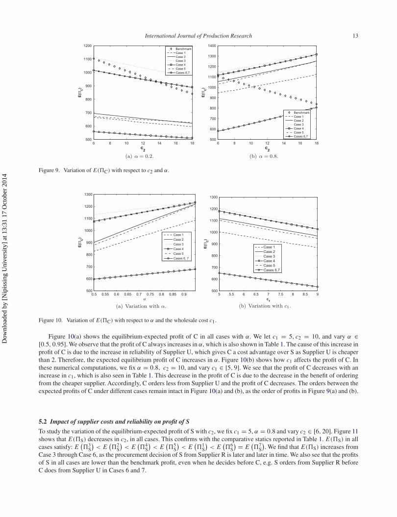
Figure 9(a) and (b) shows the equilibrium-expected profit of C with respect to c2 for low and high values of α, respectively.For computing E(�C), we let c1 = 5 and vary c2 ∈ [6, 18]. First, we see in Figure 9(a) that when the supplier is highlyunreliable, say when α = 0.2, E(�C) is decreasing in c2. On the other hand, we see in Figure 9(b) that when the supplieris highly reliable (say α = 0.8) then an increase in the cost for S leads to an increase in the profit of C. This observationis in line with the conjecture proposed in Section 4. This dependence of the monotonicity of E(�C) with c2 on α canbe explained as follows: when Supplier U is highly reliable, there is less of a chance that C will order from SupplierR at the higher cost c3 ≥ c2. This increases C’s profitability. We also see from Figure 9 that the profits for C satisfyE

(�3

C

)> E

(�4

C

)> E

(�

2,5C

)> E

(�1

C

)> E

(�6

C

) = E(�7

C

). This is in line with Proposition 9(i). This shows that

adopting CDSS is beneficial for C as it increases his profits.

Dow

nloa

ded

by [

Nip

issi

ng U

nive

rsity

] at

13:

31 1

7 O

ctob

er 2

014

International Journal of Production Research 13

Figure 9. Variation of E(�C) with respect to c2 and α.

Figure 10. Variation of E(�C) with respect to α and the wholesale cost c1.

Figure 10(a) shows the equilibrium-expected profit of C in all cases with α. We let c1 = 5, c2 = 10, and vary α ∈[0.5, 0.95]. We observe that the profit of C always increases in α, which is also shown in Table 1. The cause of this increase inprofit of C is due to the increase in reliability of Supplier U, which gives C a cost advantage over S as Supplier U is cheaperthan 2. Therefore, the expected equilibrium profit of C increases in α. Figure 10(b) shows how c1 affects the profit of C. Inthese numerical computations, we fix α = 0.8, c2 = 10, and vary c1 ∈ [5, 9]. We see that the profit of C decreases with anincrease in c1, which is also seen in Table 1. This decrease in the profit of C is due to the decrease in the benefit of orderingfrom the cheaper supplier. Accordingly, C orders less from Supplier U and the profit of C decreases. The orders between theexpected profits of C under different cases remain intact in Figure 10(a) and (b), as the order of profits in Figure 9(a) and (b).

5.2 Impact of supplier costs and reliability on profit of S

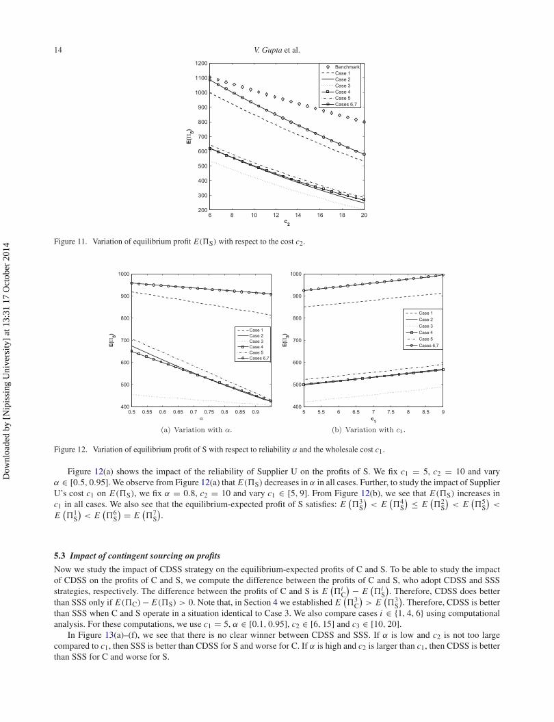
To study the variation of the equilibrium-expected profit of S with c2, we fix c1 = 5, α = 0.8 and vary c2 ∈ [6, 20]. Figure 11shows that E(�S) decreases in c2, in all cases. This confirms with the comparative statics reported in Table 1. E(�S) in allcases satisfy: E

(�3

S

)< E

(�2

S

)< E

(�4

S

)< E

(�5

S

)< E

(�1

S

)< E

(�6

S

) = E(�7

S

). We find that E(�S) increases from

Case 3 through Case 6, as the procurement decision of S from Supplier R is later and later in time. We also see that the profitsof S in all cases are lower than the benchmark profit, even when he decides before C, e.g. S orders from Supplier R beforeC does from Supplier U in Cases 6 and 7.

Dow

nloa

ded

by [

Nip

issi

ng U

nive

rsity

] at

13:

31 1

7 O

ctob

er 2

014

14 V. Gupta et al.

Figure 11. Variation of equilibrium profit E(�S) with respect to the cost c2.

Figure 12. Variation of equilibrium profit of S with respect to reliability α and the wholesale cost c1.

Figure 12(a) shows the impact of the reliability of Supplier U on the profits of S. We fix c1 = 5, c2 = 10 and varyα ∈ [0.5, 0.95]. We observe from Figure 12(a) that E(�S) decreases in α in all cases. Further, to study the impact of SupplierU’s cost c1 on E(�S), we fix α = 0.8, c2 = 10 and vary c1 ∈ [5, 9]. From Figure 12(b), we see that E(�S) increases inc1 in all cases. We also see that the equilibrium-expected profit of S satisfies: E

(�3

S

)< E

(�4

S

) ≤ E(�2

S

)< E

(�5

S

)<

E(�1

S

)< E

(�6

S

) = E(�7

S

).

5.3 Impact of contingent sourcing on profits

Now we study the impact of CDSS strategy on the equilibrium-expected profits of C and S. To be able to study the impactof CDSS on the profits of C and S, we compute the difference between the profits of C and S, who adopt CDSS and SSSstrategies, respectively. The difference between the profits of C and S is E

(�i

C

) − E(�i

S

). Therefore, CDSS does better

than SSS only if E(�C) − E(�S) > 0. Note that, in Section 4 we established E(�3

C

)> E

(�3

S

). Therefore, CDSS is better

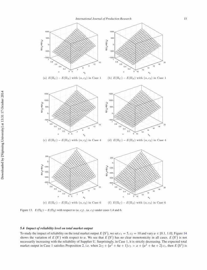
than SSS when C and S operate in a situation identical to Case 3. We also compare cases i ∈ {1, 4, 6} using computationalanalysis. For these computations, we use c1 = 5, α ∈ [0.1, 0.95], c2 ∈ [6, 15] and c3 ∈ [10, 20].

In Figure 13(a)–(f), we see that there is no clear winner between CDSS and SSS. If α is low and c2 is not too largecompared to c1, then SSS is better than CDSS for S and worse for C. If α is high and c2 is larger than c1, then CDSS is betterthan SSS for C and worse for S.

Dow

nloa

ded

by [

Nip

issi

ng U

nive

rsity

] at

13:

31 1

7 O

ctob

er 2

014

International Journal of Production Research 15

Figure 13. E(�C) − E(�S) with respect to (α, c2) , (α, c3) under cases 1,4 and 6.

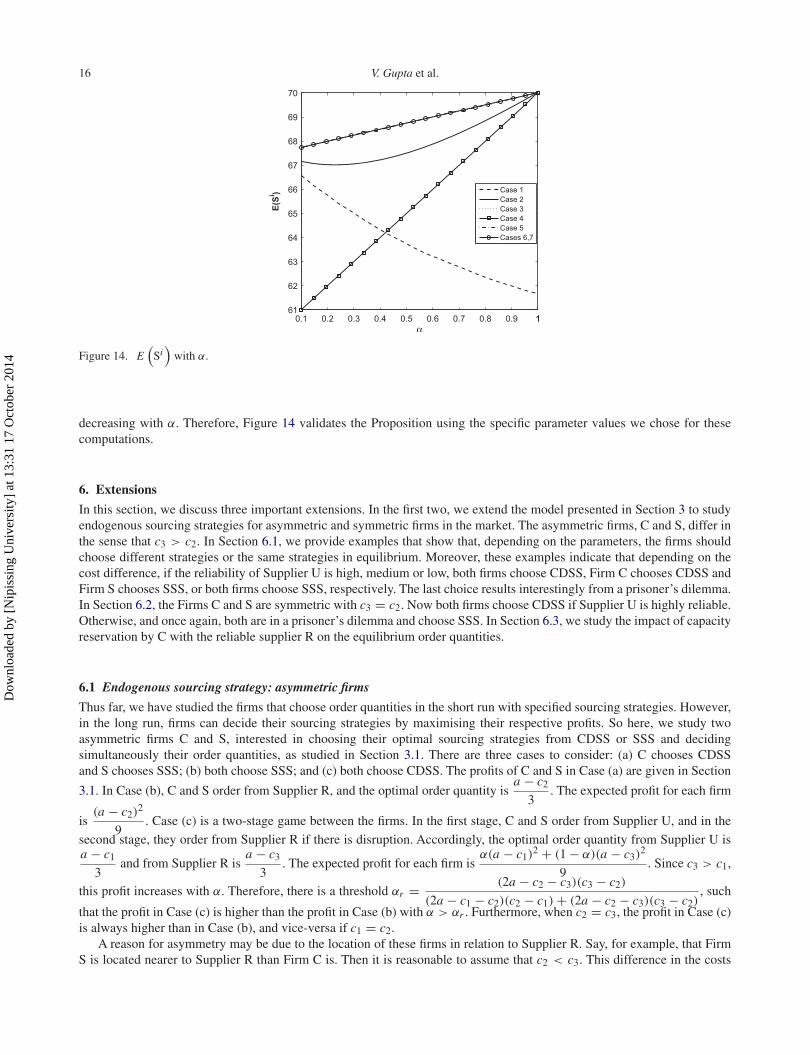
5.4 Impact of reliability level on total market output

To study the impact of reliability on the total market output E(Si

), we set c1 = 5, c2 = 10 and vary α ∈ [0.1, 1.0]. Figure 14

shows the variation of E(Si

)with respect to α. We see that E

(Si

)has no clear monotonicity in all cases. E

(Si

)is not

necessarily increasing with the reliability of Supplier U. Surprisingly, in Case 1, it is strictly decreasing. The expected totalmarket output in Case 1 satisfies Proposition 2, i.e. when 2c2 + (

α2 + 4α + 1)

c3 > a + (α2 + 4α + 2

)c1, then E

(S1

)is

Dow

nloa

ded

by [

Nip

issi

ng U

nive

rsity

] at

13:

31 1

7 O

ctob

er 2

014

16 V. Gupta et al.

Figure 14. E(

Si)

with α.

decreasing with α. Therefore, Figure 14 validates the Proposition using the specific parameter values we chose for thesecomputations.

6. Extensions

In this section, we discuss three important extensions. In the first two, we extend the model presented in Section 3 to studyendogenous sourcing strategies for asymmetric and symmetric firms in the market. The asymmetric firms, C and S, differ inthe sense that c3 > c2. In Section 6.1, we provide examples that show that, depending on the parameters, the firms shouldchoose different strategies or the same strategies in equilibrium. Moreover, these examples indicate that depending on thecost difference, if the reliability of Supplier U is high, medium or low, both firms choose CDSS, Firm C chooses CDSS andFirm S chooses SSS, or both firms choose SSS, respectively. The last choice results interestingly from a prisoner’s dilemma.In Section 6.2, the Firms C and S are symmetric with c3 = c2. Now both firms choose CDSS if Supplier U is highly reliable.Otherwise, and once again, both are in a prisoner’s dilemma and choose SSS. In Section 6.3, we study the impact of capacityreservation by C with the reliable supplier R on the equilibrium order quantities.

6.1 Endogenous sourcing strategy: asymmetric firms

Thus far, we have studied the firms that choose order quantities in the short run with specified sourcing strategies. However,in the long run, firms can decide their sourcing strategies by maximising their respective profits. So here, we study twoasymmetric firms C and S, interested in choosing their optimal sourcing strategies from CDSS or SSS and decidingsimultaneously their order quantities, as studied in Section 3.1. There are three cases to consider: (a) C chooses CDSSand S chooses SSS; (b) both choose SSS; and (c) both choose CDSS. The profits of C and S in Case (a) are given in Section

3.1. In Case (b), C and S order from Supplier R, and the optimal order quantity isa − c2

3. The expected profit for each firm

is(a − c2)

2

9. Case (c) is a two-stage game between the firms. In the first stage, C and S order from Supplier U, and in the

second stage, they order from Supplier R if there is disruption. Accordingly, the optimal order quantity from Supplier U isa − c1

3and from Supplier R is

a − c3

3. The expected profit for each firm is

α(a − c1)2 + (1 − α)(a − c3)

2

9. Since c3 > c1,

this profit increases with α. Therefore, there is a threshold αr = (2a − c2 − c3)(c3 − c2)

(2a − c1 − c2)(c2 − c1) + (2a − c2 − c3)(c3 − c2), such

that the profit in Case (c) is higher than the profit in Case (b) with α > αr . Furthermore, when c2 = c3, the profit in Case (c)is always higher than in Case (b), and vice-versa if c1 = c2.

A reason for asymmetry may be due to the location of these firms in relation to Supplier R. Say, for example, that FirmS is located nearer to Supplier R than Firm C is. Then it is reasonable to assume that c2 < c3. This difference in the costs

Dow

nloa

ded

by [

Nip

issi

ng U

nive

rsity

] at

13:

31 1

7 O

ctob

er 2

014

International Journal of Production Research 17

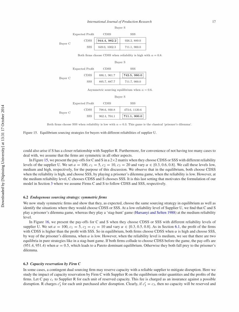
Figure 15. Equilibrium sourcing strategies for buyers with different reliabilities of supplier U.

could also arise if S has a closer relationship with Supplier R. Furthermore, for convenience of not having too many cases todeal with, we assume that the firms are symmetric in all other aspects.

In Figure 15, we present the pay-offs for C and S in a 2×2 matrix when they choose CDSS or SSS with different reliabilitylevels of the supplier U. We set a = 100, c1 = 5, c2 = 10, c3 = 20 and vary α ∈ {0.3, 0.6, 0.8}. We call these levels low,medium and high, respectively, for the purpose of this discussion. We observe that in the equilibrium, both choose CDSSwhen the reliability is high, and choose SSS, by playing a prisoner’s dilemma game, when the reliability is low. However, atthe medium reliability level, C chooses CDSS and S chooses SSS. It is this last setting that motivates the formulation of ourmodel in Section 3 where we assume Firms C and S to follow CDSS and SSS, respectively.

6.2 Endogenous sourcing strategy: symmetric firms

We now study symmetric firms and show that they, as expected, choose the same sourcing strategy in equilibrium as well asidentify the situations where they would choose CDSS or SSS. At a low-reliability level of Supplier U, we find that C and Splay a prisoner’s dilemma game, whereas they play a ‘stag-hunt’ game (Harsanyi and Selten 1988) at the medium reliabilitylevel.

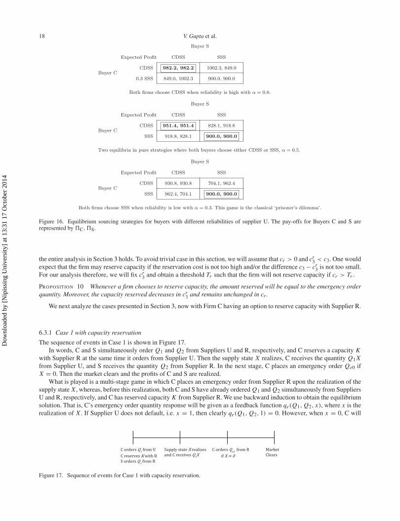
In Figure 16, we present the pay-offs for C and S when they choose CDSS or SSS with different reliability levels ofsupplier U. We set a = 100, c1 = 5, c2 = c3 = 10 and vary α ∈ {0.3, 0.5, 0.8}. As in Section 6.1, the profit of the firmswith CDSS is higher than the profit with SSS. So in equilibrium, both firms choose CDSS when α is high and choose SSS,by way of the prisoner’s dilemma, when α is low. However, when the reliability level is medium, we see that there are twoequilibria in pure strategies like in a stag-hunt game. If both firms collude to choose CDSS before the game, the pay-offs are(951.4, 951.4) when α = 0.5, which leads to a Pareto dominant equilibrium. Otherwise they both fall prey to the prisoner’sdilemma.

6.3 Capacity reservation by Firm C

In some cases, a contingent dual sourcing firm may reserve capacity with a reliable supplier to mitigate disruption. Here westudy the impact of capacity reservation by Firm C with Supplier R on the equilibrium order quantities and the profits of thefirms. Let C pay cr to Supplier R for each unit of reserved capacity. This fee is charged as an insurance against a possibledisruption. R charges cr

3 for each unit purchased after disruption. Clearly, if cr3 = c3, then no capacity will be reserved and

Dow

nloa

ded

by [

Nip

issi

ng U

nive

rsity

] at

13:

31 1

7 O

ctob

er 2

014

18 V. Gupta et al.

Figure 16. Equilibrium sourcing strategies for buyers with different reliabilities of supplier U. The pay-offs for Buyers C and S arerepresented by �C, �S.

the entire analysis in Section 3 holds. To avoid trivial case in this section, we will assume that cr > 0 and cr3 < c3. One would

expect that the firm may reserve capacity if the reservation cost is not too high and/or the difference c3 − cr3 is not too small.

For our analysis therefore, we will fix cr3 and obtain a threshold Tr such that the firm will not reserve capacity if cr > Tr .

Proposition 10 Whenever a firm chooses to reserve capacity, the amount reserved will be equal to the emergency orderquantity. Moreover, the capacity reserved decreases in cr

3 and remains unchanged in cr .

We next analyze the cases presented in Section 3, now with Firm C having an option to reserve capacity with Supplier R.

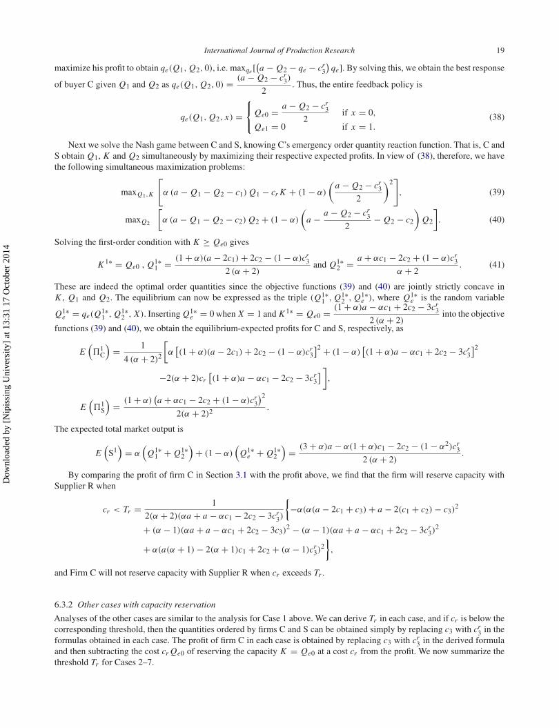
6.3.1 Case 1 with capacity reservation

The sequence of events in Case 1 is shown in Figure 17.In words, C and S simultaneously order Q1 and Q2 from Suppliers U and R, respectively, and C reserves a capacity K

with Supplier R at the same time it orders from Supplier U. Then the supply state X realizes, C receives the quantity Q1 Xfrom Supplier U, and S receives the quantity Q2 from Supplier R. In the next stage, C places an emergency order Qe0 ifX = 0. Then the market clears and the profits of C and S are realized.

What is played is a multi-stage game in which C places an emergency order from Supplier R upon the realization of thesupply state X , whereas, before this realization, both C and S have already ordered Q1 and Q2 simultaneously from SuppliersU and R, respectively, and C has reserved capacity K from Supplier R. We use backward induction to obtain the equilibriumsolution. That is, C’s emergency order quantity response will be given as a feedback function qe(Q1, Q2, x), where x is therealization of X . If Supplier U does not default, i.e. x = 1, then clearly qe(Q1, Q2, 1) = 0. However, when x = 0, C will

Figure 17. Sequence of events for Case 1 with capacity reservation.

Dow

nloa

ded

by [

Nip

issi

ng U

nive

rsity

] at

13:

31 1

7 O

ctob

er 2

014

International Journal of Production Research 19

maximize his profit to obtain qe(Q1, Q2, 0), i.e. maxqe [(a − Q2 − qe − cr

3

)qe]. By solving this, we obtain the best response

of buyer C given Q1 and Q2 as qe(Q1, Q2, 0) = (a − Q2 − cr3)

2. Thus, the entire feedback policy is

qe(Q1, Q2, x) =⎧⎨⎩ Qe0 = a − Q2 − cr

3

2if x = 0,

Qe1 = 0 if x = 1.(38)

Next we solve the Nash game between C and S, knowing C’s emergency order quantity reaction function. That is, C andS obtain Q1, K and Q2 simultaneously by maximizing their respective expected profits. In view of (38), therefore, we havethe following simultaneous maximization problems:

maxQ1,K

[α (a − Q1 − Q2 − c1) Q1 − cr K + (1 − α)

(a − Q2 − cr

3

2

)2], (39)

maxQ2

[α (a − Q1 − Q2 − c2) Q2 + (1 − α)

(a − a − Q2 − cr

3

2− Q2 − c2

)Q2

]. (40)

Solving the first-order condition with K ≥ Qe0 gives

K 1∗ = Qe0 , Q1∗1 = (1 + α)(a − 2c1) + 2c2 − (1 − α)cr

3

2 (α + 2)and Q1∗

2 = a + αc1 − 2c2 + (1 − α)cr3

α + 2. (41)

These are indeed the optimal order quantities since the objective functions (39) and (40) are jointly strictly concave inK , Q1 and Q2. The equilibrium can now be expressed as the triple (Q1∗

1 , Q1∗2 , Q1∗

e ), where Q1∗e is the random variable

Q1∗e = qe(Q1∗

1 , Q1∗2 , X). Inserting Q1∗

e = 0 when X = 1 and K 1∗ = Qe0 = (1 + α)a − αc1 + 2c2 − 3cr3

2 (α + 2)into the objective

functions (39) and (40), we obtain the equilibrium-expected profits for C and S, respectively, as

E(�1

C

)= 1

4 (α + 2)2

[α

[(1 + α)(a − 2c1) + 2c2 − (1 − α)cr

3

]2 + (1 − α)[(1 + α)a − αc1 + 2c2 − 3cr

3

]2

−2(α + 2)cr[(1 + α)a − αc1 − 2c2 − 3cr

3

] ],

E(�1

S

)= (1 + α)

(a + αc1 − 2c2 + (1 − α)cr

3

)2

2(α + 2)2.

The expected total market output is

E(

S1)

= α(

Q1∗1 + Q1∗

2

)+ (1 − α)

(Q1∗

e + Q1∗2

)= (3 + α)a − α(1 + α)c1 − 2c2 − (1 − α2)cr

3

2 (α + 2).

By comparing the profit of firm C in Section 3.1 with the profit above, we find that the firm will reserve capacity withSupplier R when

cr < Tr = 1

2(α + 2)(αa + a − αc1 − 2c2 − 3cr3)

{−α(α(a − 2c1 + c3) + a − 2(c1 + c2) − c3)

2

+ (α − 1)(αa + a − αc1 + 2c2 − 3c3)2 − (α − 1)(αa + a − αc1 + 2c2 − 3cr

3)2

+ α(a(α + 1) − 2(α + 1)c1 + 2c2 + (α − 1)cr3)

2},

and Firm C will not reserve capacity with Supplier R when cr exceeds Tr .

6.3.2 Other cases with capacity reservation

Analyses of the other cases are similar to the analysis for Case 1 above. We can derive Tr in each case, and if cr is below thecorresponding threshold, then the quantities ordered by firms C and S can be obtained simply by replacing c3 with cr

3 in theformulas obtained in each case. The profit of firm C in each case is obtained by replacing c3 with cr

3 in the derived formulaand then subtracting the cost cr Qe0 of reserving the capacity K = Qe0 at a cost cr from the profit. We now summarize thethreshold Tr for Cases 2–7.

Dow

nloa

ded

by [

Nip

issi

ng U

nive

rsity

] at

13:

31 1

7 O

ctob

er 2

014

20 V. Gupta et al.

Case 2:

Tr = 1

2(a(α + 1)(α + 2) + α(−2(α + 1)c1 + 2c2 + (α − 3)cr3) + 4c2 − 6cr

3){−2α3

(a2 − a(3c1 − 2c2 + c3) + 2c2

1 + c1(5c3 − 6c2) + 4c3(c2 − c3))

(a2 + a(6c3 − 8c1) + 8c2

1 − 4c1(c2 + c3) + c3(4c2 − 3c3))

+2α3(

a2 − a(3c1 − 2c2 + cr3) + 2c2

1 + c1(5cr3 − 6c2) + 4cr

3(c2 − cr3)

)(

a2 + a(6cr3 − 8c1) + 8c2

1 − 4c1(c2 + cr3) + cr

3(4c2 − 3cr3)

)+2α3(c1 − c3)(a − 2c1 + c3) + 2α3(cr

3 − c1)(a − 2c1 + cr3) − (a + 2c2 − 3c3)

2 + (a + 2c2 − 3cr3)

2}.

Cases 3 and 5: Tr = (1 − α)(c3 − cr3)(a + c2 − c3 − cr

3)

a + c2 − 2cr3

.

Case 4: Tr = 4(1 − α)(c3 − cr3)(a + c2 − c3 − cr

3)

3(a + c2 − 2cr3)

.

Cases 6 and 7: Tr = (1 − α)(c3 − cr3)(6a − 10αc1 + 12c2 + (5α − 9)(c3 − cr

3))

4(a − αc1 + 2c2 + (α − 3)cr3)

.

7. Conclusion

We have presented and analyzed a framework to study contingent dual sourcing strategy (CDSS) and sole sourcing strategy(SSS) under competition and supply disruption. We find that the realized supply state of an unreliable supplier and thecompetitor’s time to place an order are critical to the profits of a buyer that operates under supply disruption. Since a buyercannot control the supply disruption, we propose that he orders at a strategic time that effectively mitigates the negativeeffects of the supply disruption on his profit. Various managerial insights from the analysis, profit comparisons, computationsand study of extensions are summarized below:

• Even though CDSS has a cost advantage over SSS, it does not necessarily dominate SSS. The cost advantage ofCDSS depends also on how reliable the cheaper, unreliable supplier is. That is, when his reliability level is high, thecost advantage can be significant, making CDSS a better approach. On the other hand, when the reliability is low,SSS can be a superior strategy.

• It is interesting as well as surprising that for a firm using either sourcing strategy, the maximum profit is in the casewhen he places the order before his competitor (who adopts the other strategy) does.

• Conventional sourcing predicts that the expected total market output in a monopoly should increase with the reliabilitylevel of the supplier. However, there is a scenario (Case 1) in which the expected total competitive market outputdecreases as the reliability level of the supplier increases.

• In equilibrium, asymmetric firms with different sourcing costs may choose different sourcing strategies dependingon the reliability level of the unreliable supplier.

• In equilibrium, symmetric firms choose the same sourcing strategy. Specifically, when the reliability of the unreliablesupplier is high and his costs are sufficiently low, the firms choose CDSS, otherwise they choose SSS.

• When CDSS is adopted with a capacity reservation with the reliable supplier, the optimal capacity to reserve is equalto his emergency order quantity.

• With capacity reservation, we derive the thresholds for per unit capacity reservation cost above which the CDSSfirm does not reserve capacity.

There are possible future extensions of our research that are worth considering. One is a study of the competitive buyingbehavior with CDSS and SSS when suppliers have capacity limits. As a result, the buyers may not be able to order up to thelevel that they could without the capacity limits. This would mean that having the suppliers with limited capacities will haveimplications on the strategy of the buyers, and these will be worth examining. A more detailed study of endogenous sourcingthan that carried out in Section 6.1 would reveal how the cost asymmetry and the reliability level of the unreliable suppliersinteract. Specifically, what is the threshold level of the unreliability for the choice of different strategies given the sourcingcosts.

Dow

nloa

ded

by [

Nip

issi

ng U

nive

rsity

] at

13:

31 1

7 O

ctob

er 2

014

International Journal of Production Research 21

FundingThis work is supported by the National Natural Science Foundation of China [grant number 71001111].

References

Basar, T., and J. Olsder. 1999. Dynamic Noncooperative Game Theory. 2nd ed. Philadelphia, PA: Society for Industrial and AppliedMathematics.

Bensoussan, C., S. Chen, and S. P. Sethi. 2014. “Feedback Stackelberg Solutions of Infinite-horizon Stochastic Differential Games.” InModels and Methods in Economics and Management Sciences, Essays in Honor of Charles S. Tapiero, edited by Fouad El Ouardighiand Konstantin Kogan, 6161, Vol. 198, 3–15. Switzerland: Springer International.

Chopra, S., G. Reinhardt, and U. Mohan. 2007. “The Importance of Decoupling Recurrent and Disruption Risks in a Supply Chain.” NavalResearch Logistics 54 (5): 544–555.

Dada, M., N. C. Petruzzi, and L. S. Schwarz. 2007. “C Newsvendor’s Procurement Problem when Suppliers are Unreliable.” Manufacturingand Service Operations Management 9 (1): 9–32.

Dolgui, C., and M. C. Ould-Louly. 2002. “AModel for Supply Planning under Lead Time Uncertainty.” International Journal of ProductionEconomics 78 (2): 145–152.

Gurnani, H., S. Ray, and C. Mehrotra. 2012. Supply Chain Disruptions: Theory and Practice of Managing Risk. London: Springer-Verlag.Ha, C. Y., and S. Tong. 2008. “Contracting and Information Sharing under Supply Chain Competition.” Management science 54 (4):

701–715.Harsanyi, J. C., and R. Selten. 1988. A General Theory of Equilibrium Selection in Games. Vol. 1. Cambridge: MIT Press Books.Kazaz, S. 2004. “Production Planning under Yield and Demand Uncertainty with Yield-dependent Cost and Price.” Manufacturing and

Service Operations Management 6 (3): 209–224.Li, T., S. P. Sethi, and J. Zhang. 2013a. “Supply Diversification with Responsive Pricing.” Production and Operations Management 22

(2): 447–458.Li, T., S. P. Sethi, and J. Zhang. 2013b. “How does Pricing Power Affect a Firm’s Sourcing Decisions from Unreliable Suppliers?”

International Journal of Production Research 51 (23–24): 6990–7005.Li, J., S. Wang, and T. E. Cheng. 2010. “Competition and Cooperation in a Single-retailer Two-supplier Supply Chain with Supply

Disruption.” International Journal of Production Economics 124 (1): 137–150.Mills, E. S. 1959. “Uncertainty and Price Theory.” The Quarterly Journal of Economics 73 (1): 116–130.Mills, E. S. 1962. Price, Output, and Inventory Policy: A Study in the Economics of the Firm and Industry. Vol. 7 . New York: Wiley.Shou, S., J. Huang, and Z. Li. 2009. Managing Supply Uncertainty Under Chain-to-Chain Competition. Working Paper, City University

of Hong Kong.Snyder, L. V., Z. Atan, P. Peng, Y. Rong, A. Schmitt, and B. Sinsoysal. 2012. OR/MS Models for Supply Chain Disruptions: A Review.

Working paper. http://ssrn.com/abstract=1689882.Tang, S., and P. Kouvelis. 2011. “Supplier Diversification Strategies in the Presence of Yield Uncertainty and Buyer Competition.”

Manufacturing and Service Operations Management. 13 (4): 439–451.Tomlin, S. 2006. “On the Value of Mitigation and Contingency Strategies for Managing Supply Chain Disruption Risks.” Management

Science 52 (5): 639–657.Tomlin, S. 2009. “The Impact of Supply Learning when Suppliers are Unreliable.” Manufacturing and Service Operations Management

11 (2): 192–209.Tomlin, S. T., and L. V. Snyder. 2006. On the Value of a Threat Advisory System for Managing Supply Chain Disruptions. Working Paper.

Kenan-Flagler Business School, University of North Carolina, Chapel Hill, USA.Wang, Y., W. Gilland, and S. Tomlin. 2010. “Mitigating Supply Risk: Dual Sourcing or Process Improvement.” Manufacturing and Service

Operations Management 12 (3): 489-510.Whitin, T. M. 1995. “Inventory Control and Price Theory.” Management Science 2 (1): 61–68.

Appendix: Proofs and Supplementary Explanations

Proof of Proposition 1 The derivatives of Q1∗1 with respect to α, c1, c2 and c3, respectively, are

∂ Q1∗1

∂α= a − 2c1 − 2c2 + 3c3

2 (α + 2)2> 0,

∂ Q1∗1

∂c1= −α + 1

α + 2< 0,

∂ Q1∗1

∂c2= 1

(α + 2)> 0, and

∂ Q1∗1

∂c3= −1 − α

α + 2< 0. Similarly, we can prove the results for Q1∗

2 and Q1∗e . �

Proof of Proposition 2∂ E

(S1

)∂α

=−a −

(α2 + 4α + 2

)c1 + 2c2 +

(α2 + 4α + 1

)c3

2 (α + 2)2. So, if 2c2 +

(α2 + 4α + 1

)c3 > a +

(α2 + 4α + 2

)c1, we have

∂ E(

S1)

∂α> 0. It is easy to verify that

∂ E(

S1)

∂c1< 0,

∂ E(

S1)

∂c2< 0, and

∂ E(

S1)

∂c3< 0. �

Dow

nloa

ded

by [

Nip

issi

ng U

nive

rsity

] at

13:

31 1

7 O

ctob

er 2

014

22 V. Gupta et al.

Proof of Proposition 3

∂ E(

S2)

∂α= 1(

3α + 4 + α2)2

(6c2 − c3 + a(−1 + α(2 + α)) − c1(1 + α)(4 + α(12 + α(5 + α)))

+ α(4c2 + c3(10 + α(16 + α(6 + α))))).

If 6c2 − c3 + a(−1 +α(2 +α))− c1(1 +α)(4 +α(12 +α(5 +α)))+α(4c2 + c3(10 +α(16 +α(6 +α)))) > 0, then∂ E

(S2

)∂α

> 0.

It is easy to verify that∂ E

(S2

)∂c1

< 0,∂ E

(S2

)∂c2

< 0 and∂ E

(S2

)∂c3

< 0. �

Proof of Proposition 4∂ E

(S3

)∂α

= c3 − c1

2> 0. Therefore, the expected total market output E

(S3

)is increasing in α. Similarly, we

can prove the other results for E(

S3)

and E(

p3)

. �

Proof of Proposition 5∂ E

(S4

)∂α

= a − 6c1 + c2 + 4c3

12> 0. Therefore, the expected total market output E

(S3

)is increasing in α.

Similarly, we can prove other results for E(

S4)

and E(

p4)

. �

Proof of Proposition 6 Proposition 6 is easily derived from the first derivative of E(

S5)

and E(

p5)

with respect to α, c1, c2, and c3,respectively. �Proof of Proposition 7 We can prove this result by taking the first derivatives of E

(S6

)and E(p6) with respect to α, c1, c2, and c3,

respectively. �Proof of Proposition 8 By straightforward comparison of the profit expressions obtained in Section 3. �

Proof of Proposition 9 We have from the expected profits calculated before and c2 = c3 that E(�5

C

)> α

(a − c2)2

8+(1 − α)

(a − c2)2

16

and E(�5

S

)< α

(a − c2)2

16+ (1 − α)

(a − c2)2

8. Substituting α = 0.5 in both inequalities we have E

(�5

C

)>

3 (a − c2)2

32and

E(�5

S

)<

3 (a − c2)2

32. Therefore, E

(�5

C

)> E

(�5

S

), which completes the proposition. This means that when Supplier U is sufficiently

reliable, i.e. α ≥ 0.5, C has a higher expected profit than S. �Proof of Proposition 10 Let the capacity reserved by C be K ∗(cr ), and the emergency order quantity at cr be Qk∗

e (cr ). Correspondingly,there are three cases – (a) K ∗(cr ) > Qk∗

e (cr ); (b) K ∗(cr ) < Qk∗e (cr ); and (c) K ∗(cr ) = Qk∗

e (cr ). In Case (a); the reserved capacity ishigher than the emergency order quantity. C saves cr (K ∗(cr ) − Qk∗

e (cr )) by reserving a capacity of Qk∗e (cr ). Therefore, it is not optimal

for C to choose K ∗(cr ) > Qk∗e (cr ). On the other hand, in Case (b) the reserved capacity K ∗(cr ) is less than Qk∗

e (cr ). Therefore, C cannotfulfil the optimal emergency order. Therefore, it is not optimal for C to choose K ∗(cr ) < Qk∗

e (cr ). Therefore, K ∗(cr ) = Qk∗e (cr ) is

optimal for C. From Section 3.1, we see that Qk∗e decreases in cr

3 and cr is a sunk cost to decide Qk∗e . �

Dow

nloa

ded

by [

Nip

issi

ng U

nive

rsity

] at

13:

31 1

7 O

ctob

er 2

014