Contribution for Innovations in Financial and Economic ... · Contribution for Innovations in Financial and Economic Networks Anna Nagurney, editor ... Department of Economics Iowa

Contribution for

Innovations in Financial

and Economic Networks

Anna Nagurney, editor

Mark PingleDepartment of Economics

University of NevadaReno, NV 89557-0016

http://unr.edu/homepage/pingle/[email protected]

Leigh TesfatsionDepartment of Economics

Iowa State UniversityAmes, IA 50011-1070

http://www.econ.iastate.edu/tesfatsi/[email protected]

April 11, 2003

1 Evolution of

Worker-Employer

Networks and Behaviors

Under Alternative

Non-Employment Benefits:

An Agent-Based

Computational StudyMark Pingle and Leigh Tesfatsion

1.1 Introduction

Determining the effects of labor institutions on macroeconomic performanceis a central concern of economic policymakers. Differences in labor insti-tutions have been conjectured to be a key explanation for observed cross-country differences in the level and persistence of unemployment, in the dis-tribution of income and wealth, and in growth rates for labor productivityand GDP.

For example, as discussed by Blau and Kahn (1999), Ljungqvist and Sar-gent (1998), and Nickell and Layard (1999), European OECD countries overthe past twenty years have tended to rely on administered wages and leg-islated job protection and have experienced sluggish job growth and persis-tently high unemployment. In contrast, the United States has had a relatively

2 1 Evolution of Worker-Employer Networks and Behaviors Under Alternative Non-Employment Benefits: An Agent-Based Computational Study

more flexible, less regulated labor market and has achieved much greater jobgrowth and relatively lower unemployment rates. This has led many Euro-pean policymakers to argue the need for reforms in their labor institutions.

Unfortunately, as discussed by Acemoglu and Shimer (2000), Blau andKahn (1999), and Freeman (1998), it is difficult to obtain conclusive em-pirical results regarding how labor institutions affect economic performance.Regression methods relating changes in labor institutions to economic out-comes quickly tax degrees of freedom. This problem is compounded if oneinstitution’s impact depends on the presence or absence of other institutions.Also, labor institutions are inherently endogenous. For example, govern-ments continually revise labor institutions in response to economic and po-litical pressures. This endogeneity makes it difficult to interpret the validityof empirical investigations.

In recognition of these difficulties, Freeman (1998, pp. 19-20) suggests thatagent-based computational modeling might offer a promising additional wayto study the impact of labor institutions, particularly from a market designperspective. Tesfatsion (1998,2001,2002a) reports some preliminary workalong these lines. An agent-based computational economics (ACE) frameworkis used to study path dependence, market power, and market efficiency out-comes for a labor market under systematically varied concentration and ca-pacity conditions. ACE is the computational study of economies modeled asevolving systems of autonomous interacting agents (Tesfatsion,2002b,2003).1

In this study we conduct an ACE labor market experiment to test the sen-sitivity of labor market outcomes to changes in the level of a non-employmentpayment. Our ultimate objective is to understand how the basic features ofreal-world unemployment benefit programs affect labor market performance.2

However, as will be clarified below, a human subject experiment was run inparallel to this computational experiment as a check on the reliability of ourfindings and the adequacy of the learning representations for our computa-tional workers and employers. To facilitate this initial benchmark check, adeliberately simplified experimental design is used.

Specifically, we consider a balanced labor market with equal numbersof workers and employers. In each trade cycle (work period), every workerhas one work offer to make and every employer has one job opening to fill.An employer can reject a work offer received from a worker on two possiblegrounds: unacceptable past work history; or capacity limitations.

1See http://www.econ.iastate.edu/tesfatsi/ace.htm for extensive resources related toACE, including surveys, an annotated syllabus of readings, research area sites, software,teaching materials, and pointers to individual researchers and research groups.

2For example, in the U.S., unemployment benefits are financed by taxes on employers

and are intended to provide temporary financial assistance to workers who become unem-ployed through no fault of their own and who continue to seek work . Understanding theseparate and combined impacts of these and other unemployment benefit program featureson labor market performance over time is an extremely challenging problem. A detaileddiscussion of theoretical and empirical labor market studies focusing on unemploymentbenefits and related issues can be found in Pingle and Tesfatsion (2001).

1.1 Introduction 3

The workers repeatedly submit their work offers to preferred employersuntil either they succeed in being hired or they become discouraged by re-jections and exit the job market. A worker must pay a small transactioncost each time he submits a work offer to an employer. As in MacLeod andMalcomson (1998), each matched worker and employer individually choosesto shirk or cooperate on the work-site, and these choices are made simulta-neously so that neither has a strategic informational advantage. Any workeror employer who does not enter an employment relationship during the tradecycle in question receives an exogenously specified non-employment payment.Workers and employers evolve their work-site behaviors over time on the basisof past experiences in an attempt to increase their earnings.

In this labor market, then, full employment with no job vacancies ispossible. Nevertheless, the unemployment rate and the particular set ofworkers and employers in employment relationships endogenously evolve overthe course of successive trade cycles. Two interdependent choices made re-peatedly by the workers and the employers shape this evolutionary process:namely, their choices of work-site partners; and their behavioral choices ininteractions with these partners.

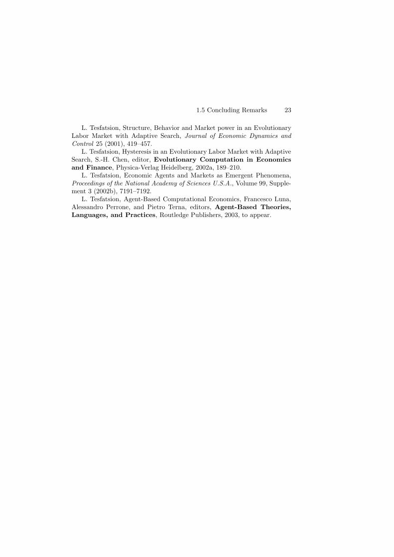
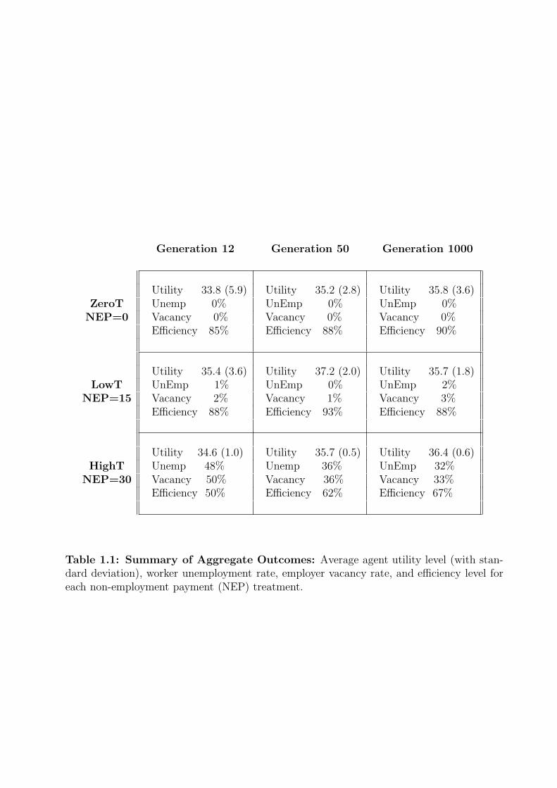
Three non-employment payment (NEP) treatments are experimentallystudied: a zero NEP; a low NEP; and a high NEP. As reported in Table 1.1,one main finding is that the average utility levels attained by workers andemployers do not substantially change as the NEP is increased from zero tohigh. As will be clarified in Section 1.4, although the increase in the NEPincreases the worker unemployment rate and the employer vacancy rate, thisgreater loss of productive activity is offset in part by the higher NEP and inpart by the increased levels of mutual cooperation exhibited by the workersand employers who manage to match.

Another main finding reported in Table 1.1 is that a somewhat higheraverage utility level for workers and employers is attained with a low NEPthan with either a zero or a high NEP in the short and intermediate runs(generations 1 through 50). As will be explained more carefully in Section 1.4,a zero NEP encourages shirking on the work-site (low risk of quits or firingsin reponse to defections) while a high NEP results in a high risk of lostearnings due to coordination failure (high risk of quits or firings in responseto defections). Interestingly, however, average utility tends to increase overtime under each NEP treatment as the workers and employers become betterat sustaining mutual cooperation on the work-site. Moreover, this movementtowards higher average utility is strongest under the high NEP treatment.Thus, in the long run (generation 1000), the average utility level attained byworkers and employers with a high NEP exceeds the average utility levelsattained with a zero or low NEP.

On the other hand, program costs should be taken into account as wellas utility benefits in order to obtain a more accurate measure of economicefficiency. Let net earnings be measured by the average (per agent) utility


level attained by workers and employers minus the average NEP paid to theseworkers and employers. Define efficiency to be the ratio of actual net earningsto maximum possible net earnings. As indicated in Table 1.1, although a highNEP results in a high average utility level, it also results in a significantlylower efficiency level than either the zero or low NEP due to high programcosts. Overall, considering the short, intermediate, and long run, the lowNEP delivers the highest overall efficiency level. Consequently, evaluated interms of efficiency, our findings indicate that a low NEP is preferable to eithera zero or a high NEP.

The aggregate outcomes reported in Table 1.1, while interesting, are onlythe tip of the iceberg. A careful study of individual experimental runs in-dicates that the response of the ACE labor market to changes in the NEPis much more intricately structured than this table suggests. As reportedin Figure 1.1, the 20 runs generated for each NEP treatment tend to grav-itate towards one of two “attractor states.” The configuration of these twoattractor states is similar under the zero and low NEP treatments: the firstattractor state is characterized by latched pairs of mutually cooperative work-ers and employers, while the second attractor state is characterized by latchedpairs of workers and employers who intermittently defect and cooperate. Incontrast, under the high NEP treatment, one attractor state is characterizedby latched pairs of mutually cooperative workers and employers while theother attractor state is a state of economic collapse in which each worker andemployer ultimately becomes inactive. This apparent existence of multipleattractor states suggests caution in interpreting the aggregate outcomes re-ported in Table 1.1, since these outcomes could be based on inappropriatelypooled data.

The existence of multiple attractor states for each NEP treatment is dueto strong network and learning effects. Starting from the same initial struc-tural conditions, chance differences in the initial interaction patterns amongthe workers and employers can cause the labor market to evolve towards per-sistent interaction networks supporting sharply distinct types of expressedbehaviors. For example, with a high NEP, the labor market evolves eithertowards a highly efficient economy in which all workers and employers arein long-run mutually cooperative relationships or towards economic collapsewith 100% unemployment. Thus, while a change in the level of the NEP canbe expected to have substantial systematic effects on key labor market out-comes such as efficiency and unemployment, our findings suggest that theseeffects will be in the form of spectral (multiple peaked) distributions withlarge standard deviations.

These computational experiment findings can be compared to findingsreported in Pingle and Tesfatsion (2002) for a human-subject experiment us-ing a similarly structured labor market but with a smaller number of workersand employers participating in a much smaller number of trade cyces perexperimental session. In the human-subject experiment, as in the computa-

1.2 The ACE Labor Market Model 5

tional experiment, a higher NEP resulted in higher average unemploymentand vacancy rates as well as higher average utility levels among those whosuccessfully matched. In the human-subject experiment, however, most rela-tionships that formed between workers and employers were either short-livedor intermittent, with only modest amounts of behavioral coordination in ev-idence. In contrast, in the computational experiment almost all workers andemployers who succeeded in matching ended up in long-run relationships withone partner in which the behaviors of the partners were highly coordinated.

As detailed more carefully in Pingle and Tesfatsion (2002), this differencein findings raises interesting questions. To what extent are the human-subjectand computational experiments capturing the same economic structure butreporting over different time scales, short run versus long run? In partic-ular, could it be that the “shadow of the past” weighs heavily on humansubjects over the necessarily shorter human-subject trials, biasing behaviorstowards unknown past points of reference? If so, the computational experi-ment might be providing the more accurate prediction of what would happenin actual labor markets over a longer span of time. Alternatively, the twoexperiments might differ structurally in some fundamental way so that differ-ences in outcomes would be observed regardless of time scale. In particular,is the representation of agent learning in the computational experiment tooinaccurate to permit valid comparisons with human-subject labor market ex-periments? Are the observed differences in types of network formations dueto the different frequencies with which transaction costs are incurred due toscale effects? Careful additional studies, both empirical and experimental,will be needed to resolve these questions.

The ACE labor market model is presented in Section 1.2. Section 1.3outlines the experimental design of our study, and Section 1.4 provides a de-tailed report of our experimental findings. Concluding remarks are presentedin Section 1.5.

1.2 The ACE Labor Market Model

Overview:

The ACE labor market comprises 12 workers and 12 employers. Eachworker can work for at most one employer at any given time, and eachemployer can employ at most one worker at any given time. The workersand employers repeatedly seek preferred work-site partners using a modifiedform of a matching mechanism (Gale-Shapley, 1962) that has been observedto evolve in various real-world labor market settings (Roth and Sotomayor,1992). The workers and employers who successfully match then engage inrisky work-site interactions modeled as prisoner’s dilemma games. At reg-ular intervals the workers and employers separately update their work-siterules of behavior on the basis of the past earnings obtained with these rules.

The computational experiment is implemented by means of the Trade


Network Game Laboratory (TNG Lab), an agent-based computational labo-ratory developed by McFadzean, Stewart, and Tesfatsion (2001) for studyingthe evolution of trade networks via real-time animations, tables, and graph-ical displays.3 The specific TNG parameter settings used for the experimentat hand are described below. All other TNG parameter settings are the sameas in Tesfatsion (2001).

Implementation Details:

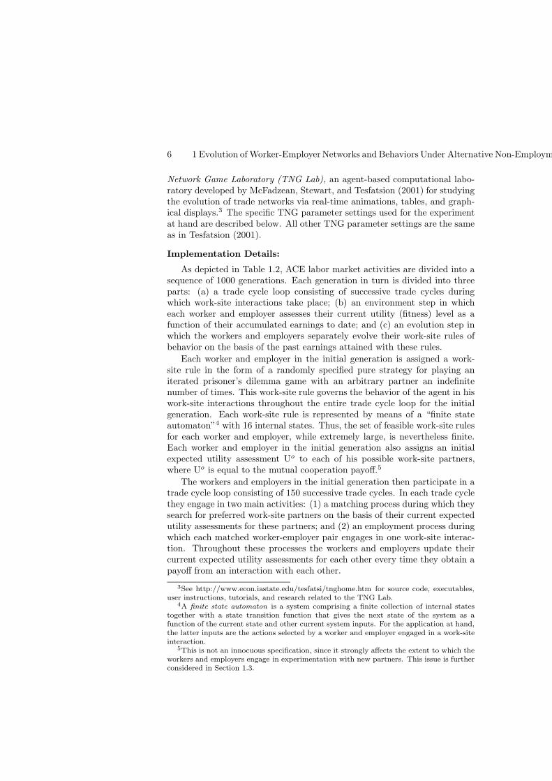
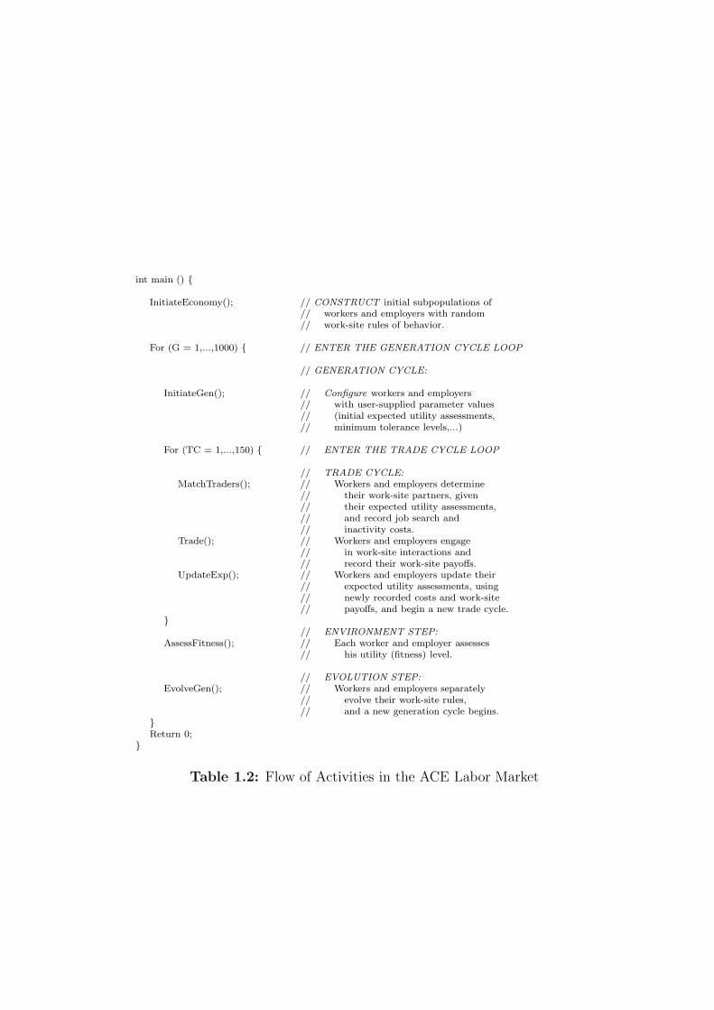
As depicted in Table 1.2, ACE labor market activities are divided into asequence of 1000 generations. Each generation in turn is divided into threeparts: (a) a trade cycle loop consisting of successive trade cycles duringwhich work-site interactions take place; (b) an environment step in whicheach worker and employer assesses their current utility (fitness) level as afunction of their accumulated earnings to date; and (c) an evolution step inwhich the workers and employers separately evolve their work-site rules ofbehavior on the basis of the past earnings attained with these rules.

Each worker and employer in the initial generation is assigned a work-site rule in the form of a randomly specified pure strategy for playing aniterated prisoner’s dilemma game with an arbitrary partner an indefinitenumber of times. This work-site rule governs the behavior of the agent in hiswork-site interactions throughout the entire trade cycle loop for the initialgeneration. Each work-site rule is represented by means of a “finite stateautomaton”4 with 16 internal states. Thus, the set of feasible work-site rulesfor each worker and employer, while extremely large, is nevertheless finite.Each worker and employer in the initial generation also assigns an initialexpected utility assessment Uo to each of his possible work-site partners,where Uo is equal to the mutual cooperation payoff.5

The workers and employers in the initial generation then participate in atrade cycle loop consisting of 150 successive trade cycles. In each trade cyclethey engage in two main activities: (1) a matching process during which theysearch for preferred work-site partners on the basis of their current expectedutility assessments for these partners; and (2) an employment process duringwhich each matched worker-employer pair engages in one work-site interac-tion. Throughout these processes the workers and employers update theircurrent expected utility assessments for each other every time they obtain apayoff from an interaction with each other.

3See http://www.econ.iastate.edu/tesfatsi/tnghome.htm for source code, executables,user instructions, tutorials, and research related to the TNG Lab.

4A finite state automaton is a system comprising a finite collection of internal statestogether with a state transition function that gives the next state of the system as afunction of the current state and other current system inputs. For the application at hand,the latter inputs are the actions selected by a worker and employer engaged in a work-siteinteraction.

5This is not an innocuous specification, since it strongly affects the extent to which theworkers and employers engage in experimentation with new partners. This issue is furtherconsidered in Section 1.3.

1.2 The ACE Labor Market Model 7

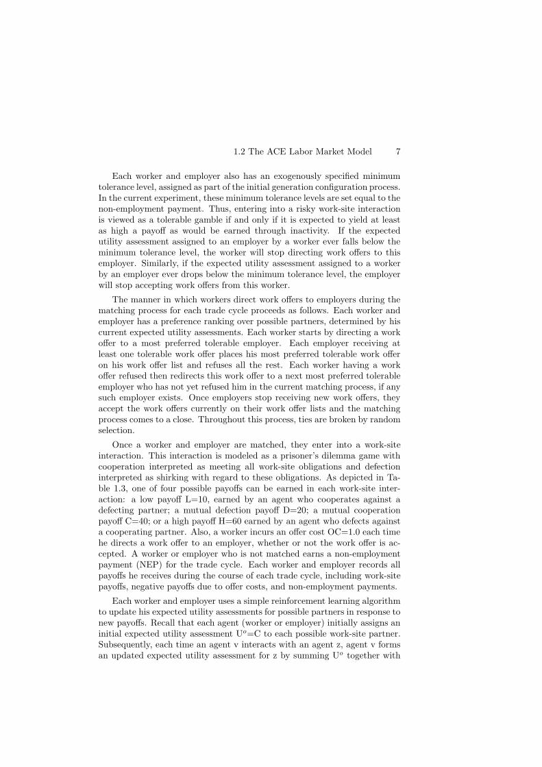
Each worker and employer also has an exogenously specified minimumtolerance level, assigned as part of the initial generation configuration process.In the current experiment, these minimum tolerance levels are set equal to thenon-employment payment. Thus, entering into a risky work-site interactionis viewed as a tolerable gamble if and only if it is expected to yield at leastas high a payoff as would be earned through inactivity. If the expectedutility assessment assigned to an employer by a worker ever falls below theminimum tolerance level, the worker will stop directing work offers to thisemployer. Similarly, if the expected utility assessment assigned to a workerby an employer ever drops below the minimum tolerance level, the employerwill stop accepting work offers from this worker.

The manner in which workers direct work offers to employers during thematching process for each trade cycle proceeds as follows. Each worker andemployer has a preference ranking over possible partners, determined by hiscurrent expected utility assessments. Each worker starts by directing a workoffer to a most preferred tolerable employer. Each employer receiving atleast one tolerable work offer places his most preferred tolerable work offeron his work offer list and refuses all the rest. Each worker having a workoffer refused then redirects this work offer to a next most preferred tolerableemployer who has not yet refused him in the current matching process, if anysuch employer exists. Once employers stop receiving new work offers, theyaccept the work offers currently on their work offer lists and the matchingprocess comes to a close. Throughout this process, ties are broken by randomselection.

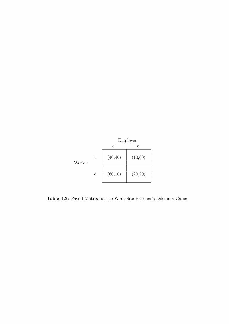
Once a worker and employer are matched, they enter into a work-siteinteraction. This interaction is modeled as a prisoner’s dilemma game withcooperation interpreted as meeting all work-site obligations and defectioninterpreted as shirking with regard to these obligations. As depicted in Ta-ble 1.3, one of four possible payoffs can be earned in each work-site inter-action: a low payoff L=10, earned by an agent who cooperates against adefecting partner; a mutual defection payoff D=20; a mutual cooperationpayoff C=40; or a high payoff H=60 earned by an agent who defects againsta cooperating partner. Also, a worker incurs an offer cost OC=1.0 each timehe directs a work offer to an employer, whether or not the work offer is ac-cepted. A worker or employer who is not matched earns a non-employmentpayment (NEP) for the trade cycle. Each worker and employer records allpayoffs he receives during the course of each trade cycle, including work-sitepayoffs, negative payoffs due to offer costs, and non-employment payments.

Each worker and employer uses a simple reinforcement learning algorithmto update his expected utility assessments for possible partners in response tonew payoffs. Recall that each agent (worker or employer) initially assigns aninitial expected utility assessment Uo=C to each possible work-site partner.Subsequently, each time an agent v interacts with an agent z, agent v formsan updated expected utility assessment for z by summing Uo together with


all payoffs received to date from interactions with z and dividing this sum byone plus the total number of these interactions. The payoffs included in thissummation include work-site payoffs and negative payoffs due to offer costs.Consequently, an updated expected utility assessment for any agent z is theaverage of all payments received to date in interactions with z, augmentedto include Uo as a virtual additional payoff. Under this method, if an agentinteracts repeatedly with another agent for a sufficient length of time, hisexpected utility assessment for z will eventually approach his true averagepayoff level from interactions with z.6

At the end of the initial generation, the workers and employers enter intoan environment step in which each agent calculates his utility (fitness) level.This utility level is taken to be the average total net payoffs per trade cyclethat the agent earned during the course of the preceding trade cycle loop, i.e.,the agent’s total net payoffs divided by 150 (the number of trade cycles perloop). The workers and employers then enter into an evolution step in whichthey use their attained utility levels to evolve (structurally update) theirwork-site rules via both inductive and social learning. Inductive learningtakes the form of experimentation; agents perturb their work-site rules byintroducing random modifications. Social learning takes the form of mimicry;agents deliberately modify their work-site rules to more closely resemble thework-site rules used by more successful (higher utility) agents of their owntype. Thus, workers imitate other more successful workers, and employersimitate other more successful employers.

Experimentation and mimicry are separately implemented for workersand for employers by means of genetic algorithms involving commonly usedelitism, mutation, and recombination operations. Elitism ensures that themost successful work-site rules are retained unchanged from one generationto the next. Mutation ensures that workers and employers continually exper-iment with new work-site rules (inductive learning). Recombination ensuresthat workers and employers continually engage in mimicry (social learning).7

At the end of the evolution step, each worker and employer has a poten-tially new work-site rule. The memory of each worker and employer is thenwiped clean of all past work-site experiences. In particular, initial expectedutility assessments for possible partners are re-set to the mutual cooperationpayoff level without regard for past work-site experiences. The workers andemployers then enter into a new generation and the whole process repeats,for a total of 1000 generations in all.8

6See McFadzean and Tesfatsion (1999) for more details. Briefly, this long-run consis-tency property follows from the finite state automaton representation for work-site ruleswhich ensures that the action pattern between any two agents who repeatedly interactmust eventually enter into a cycle as the number of their interactions becomes sufficientlylarge.

7See McFadzean and Tesfatsion (1999) and Tesfatsion (2001) for detailed discussions ofthis use of genetic algorithms to implement the evolution of work-site rules.

8A final technical remark about implementation should also be noted, in case otherswish to replicate or extend this experiment. The minimum tolerance level is hardwired

1.3 The Computational Experiment 9

1.3 The Computational Experiment

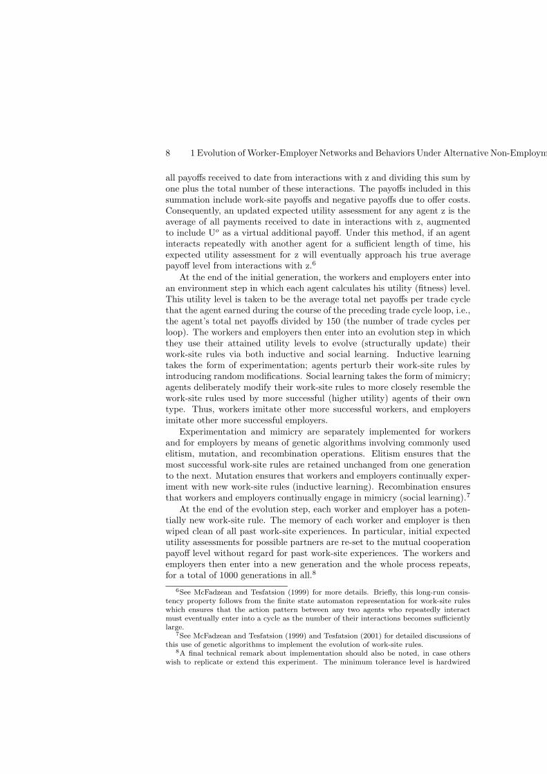
The computational experiment focuses on only one treatment variable, thenon-employment payment (NEP). The three tested treatments for NEP areNEP=0, NEP=15, and NEP=30. These three treatments are referred to asZeroT, LowT, and HighT, respectively.

The interest in these three alternative treatments is seen by comparingthem with the work-site payoffs depicted in Table 1.3. In treatment ZeroT,non-employment during a trade cycle results in the payment NEP=0. This isthe worst possible trade cycle payoff, worse even than the sucker payoff L=10that results from cooperating with a defecting work-site partner. In treatmentZeroT, then, unemployment or vacancy is never an attractive alternative toemployment or hiring, and the workers and employers will be willing to putup with defections to avoid unemployment or vacancy.

In contrast, in treatment LowT non-employment during a trade cycleresults in the payment NEP=15. This payment is strictly higher than thesucker payoff L=10, meaning agents will prefer non-employment to beingsuckered. Thus, each agent who defects against a cooperative partner to at-tain a high payoff now faces a risk of future non-employment if this currentpartner chooses not to interact with him in the future. Finally, in treatmentHighT non-employment results in the payment NEP=30. This payment dom-inates both the sucker payoff L=10 and the mutual defection payoff D=20.Consequently, agents will tend to be much more sensitive to defections, pre-ferring unemployment or vacancy in preference to defecting back against adefecting partner.

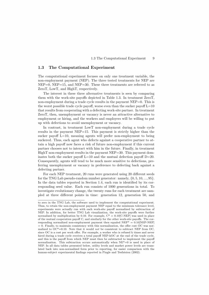
For each NEP treatment, 20 runs were generated using 20 different seedsfor the TNG Lab pseudo-random number generator: namely, {0, 5, 10, ..., 95}.In the data tables reported in Section 1.4, each run is identified by its cor-responding seed value. Each run consists of 1000 generations in total. Toinvestigate evolutionary change, the twenty runs for each treatment are sam-pled at three different points in time: generation 12, generation 50, and

to zero in the TNG Lab, the software used to implement the computational experiment.Thus, to retain the non-employment payment NEP equal to the minimum tolerance level,experiments were actually run with each work-site payoff normalized by subtraction ofNEP. In addition, for better TNG Lab visualization, the work-site payoffs were furthernormalized by multiplication by 0.10. For example, C* = 0.10[C-NEP] was used in placeof the mutual cooperation payoff C, and similarly for the other work-site payoffs. The cor-responding normalized non-employment payment then equaled NEP* = 0.10[NEP-NEP]= 0. Finally, to maintain consistency with this normalization, the offer cost OC was nor-malized to OC*=0.10. Note that it would not be consistent to subtract NEP from OC,since OC is a cost per work offer. For example, a worker who is refused k times and neverhired during a trade cycle receives a total payoff NEP-kOC at the end of the trade cycle,and this is the payoff from which NEP must then be subtracted to implement the payoffnormalization. This subtraction occurs automatically when NE*=0 is used in place ofNEP. In all data tables presented below, utility levels and market power levels are trans-lated back into non-normalized form prior to reporting, for easier comparison with thehuman-subject experimental findings reported in Pingle and Tesfatsion (2002).


generation 1000. For each sampled generation, data is collected regardingnetwork formation, market non-participation rates, work-site behaviors, wel-fare (utility and market power) outcomes, and persistent relationship typecounts.

Before reporting our experimental findings in detail, it is important toexplain carefully the descriptive statistics that have been constructed to helpcharacterize the one-to-many mapping between treatment and outcomes.

Measurement of Persistent Relationships:

As previously noted (see footnote 4), work-site rules are represented asfinite state automata, implying that the actions undertaken by any one agentin repeated work-site interactions with another agent must eventually cycle.Consequently, the actions of any one agent in interactions with another agentduring a trade cycle loop can be summarized in the form of a work-site historyH:P. The “handshake” H is a (possibly null) string of work-site actions thatform a non-repeated pattern, while the “persistent portion” P is a (possiblynull) string of work-site actions that are cyclically repeated. For example,letting c denote cooperation and d denote defection, the work-site historyddd:dc for an agent v in interactions with another agent z indicates that vdefected against z in his first three work-site interactions with z and thereafteralternated between defection and cooperation.

A worker and employer are said to exhibit a persistent relationship duringa given trade cycle loop if two conditions hold. First, their work-site historieswith each other during the course of this loop each have non-null persistentportions. Second, accepted work offers between the worker and employerdo not permanently cease during this loop either by choice (a permanentswitch away to a strictly preferred partner) or by refusal (one agent becomesintolerable to the other because of too many defections).

A persistent relationship between a worker and employer in a given tradecycle loop is said to be latched if the worker works continually for the em-ployer (i.e., in every successive trade cycle) during the persistent portions oftheir work-site histories. Otherwise, the persistent relationship is said to berecurrent .

Measurement of Market Non-Participation Rates:

A worker or employer who fails to form any persistent relationship dur-ing a given trade cycle loop is classified as persistently non-employed forthat trade cycle loop. The percentage of workers who are persistently non-employed constitutes the persistent unemployment rate for that trade cy-cle loop. Similarly, the percentage of employers who are persistently non-employed constitutes the persistent vacancy rate for that trade cycle loop.

Classification of Networks by Competitive Distance:

We will next construct a distance measure that permits the classifica-tion of experimentally observed “interaction networks” into alternative types.This distance measure will calculate the distance between an experimentally

1.3 The Computational Experiment 11

observed interaction network and an idealized interaction network capable ofsupporting a competitive (full employment) market outcome.

Recall from Table 1.2 that each generation G of the ACE labor marketmodel consists of a single trade cycle loop plus an environment step and anevolution step. The interaction network N(G,R) for a particular generationG in a particular experimental run R refers to the observed pattern of inter-actions occurring among workers and employers in the trade cycle loop forthat generation and run.

Each interaction network N(G,R) is represented in the form of a directedgraph. The vertices V of the graph represent the workers and employers.The edges of the graph (directed arrows) represent work offers directed fromworkers to employers. Finally, the edge weight on any edge denotes the num-ber of accepted work offers between the worker and employer connected bythe edge. The reduced-form network PN(G,R) derived from N(G,R) by elim-inating all edges of N(G,R) that correspond to non-persistent relationshipsis referred to as the persistent network corresponding to N(G,R).

In a standard competitive equilibrium situation, workers are indifferentamong employers offering the same working conditions and employers areindifferent among workers offering identical labor services. Moreover, workersoffering the same labor services have the same ex ante expected employmentrate and employers offering the same working conditions have the same exante expected vacancy rate.

In the current labor market model, these same market characteristicswould tend to prevail if all workers and employers always cooperated. Inthe latter case, due to indifference, workers would randomly distribute theirwork offers across all employers and employers would randomly select workoffers from among all work offers received. The resulting interaction patternwould therefore tend to be fully recurrent (no latching and no persistentnon-employment) with equal ex ante expected employment rates and vacancyrates for workers and employers, respectively. For these reasons, the followinginteraction pattern among workers and employers is referred to below as acompetitive interaction pattern: Each worker is recurrently directing workoffers to employers, and every worker and employer has at least one persistentrelationship.

The network distance for any persistent network PN(G,R) is then definedto be the number of vertices (agents) in PN(G,R) whose edges (persistentrelationships) fail to conform to the competitive interaction pattern. Byconstruction, then, a distance measure of 0 indicates zero deviation and adistance measure of 24 (the total number of workers and employers) indicatesmaximum deviation. In particular, a perfectly recurrent persistent networkhas a network distance of 0, a perfectly latched persistent network has anetwork distance of 12, and a perfectly disconnected persistent network (nopersistent relationships) has a network distance of 24.

Classification of Work-Site Behaviors:


A worker or employer in generation G of a run R is called a never-provokeddefector (NPD) if he ever defects against another agent that has not previ-ously defected against him. The percentages of workers and employers whoare NPDs measure the extent to which these agents behave opportunisticallyin work-site interactions with partners who are strangers or who so far havebeen consistently cooperative.

A worker or employer in generation G of a run R is referred to as a per-sistent intermittent defector (IntD) if he establishes at least one persistentrelationship for which his persistent portion consists of a non-trivial mix ofdefections and cooperations. The agent is referred to as a persistent defec-tor (AllD) if he establishes at least one persistent relationship and if thepersistent portion of each of his persistent relationships consists entirely ofdefections. Finally, the agent is referred to as a persistent cooperator (AllC) ifhe establishes at least one persistent relationship and if the persistent portionof each of his persistent relationships consists entirely of cooperations. Byconstruction, an agent in generation G of a run R satisfies one and only oneof the following four agent-type classifications: persistently non-employed; apersistent intermittent defector; a persistent defector; or a persistent coop-erator.

Two important points can be made about this classification of agent types.First, in contrast to standard game theory, the agents coevolve their typesover time. This coevolution is in response to past experiences, starting frominitially random behavioral specifications. Thus, agent typing is endogenous.Second, agent typing is measured in terms of persistently expressed behav-iors, not in terms of work-site rules. An agent may have coevolved into anAllC in terms of expressed behaviors with current work-site partners, basedon past work-site experiences with these partners, while still retaining thecapability of defecting against a new untried partner. Indeed, work-site rulescontinually coevolve in the evolution step through mutation and recombina-tion operations even if expressed behaviors appear to have largely stabilized.This ceaseless change in work-site rules makes any apparent stabilization inthe distribution of agent types all the more surprising and interesting.

Measurement of Utility and Market Power Outcomes:

The utility level of a worker or employer at the end of generation G in arun R is measured by the average total net payoffs per trade cycle that theagent earns during the course of the trade cycle loop for generation G.

With regard to market power, we adopt the standard industrial organi-zation approach: namely, market power is measured by the degree to whichthe actual utility levels attained by workers and employers compare againstan idealized competitive yardstick. We take as this yardstick a situation inwhich there is absence of strategic behavior, symmetric treatment of equals,and full employment. Specifically, we define competitive market conditionsfor the ACE labor market to be a situation in which each worker is recur-rently directing work offers to employers, and each worker and employer is a

1.4 Experimental Findings 13

persistent cooperator (AllC).Ignoring offer costs, the utility level that each worker and employer would

attain under these competitive market conditions is simply the mutual coop-eration payoff level, C. Therefore, as in Pingle and Tesfatsion (2001,2002), wedefine the market power (MPow) of each worker or employer in generationG of a run R to be the extent to which their attained utility level, U, differsfrom C: that is, MPow = (U-C)/C.

Classification of Persistent Relationship Types:

A persistent relationship between a worker and employer in generation Gof a run R is classified in accordance with the persistent behaviors expressedby the two participants in this particular relationship.

If both participants are persistent intermittent defectors (IntDs), the re-lationship is classified as mutual intermittent defection (M-IntD). If bothparticipants are persistent defectors (AllDs), the relationship is classified asmutual defection (M-AllD). If both participants are persistent cooperators(AllCs), the relationship is classified as mutual cooperation (M-AllC). Notethat the relative shirking rates for an M-IntD relationship can be deducedfor the participant worker and employer by examining their relative marketpower levels.

A persistent relationship in which the worker and employer express dis-tinct types of behaviors is indicated in hyphenated form, with the worker’sbehavior indicated first. For example, a persistent relationship involving aworker who is an IntD and an employer who is an AllC is indicated by theexpression IntD-AllC.

1.4 Experimental Findings

Overview:

The results for the computational experiment display a startling degreeof regularity. This regularity is visible as early as the twelfth generation andpersists through generation 1000.

For each of the three NEP treatments ZeroT, LowT, and HighT, thetwenty trial runs tend to cluster into two distinct attractor states. Each at-tractor state supports a distinct configuration of market non-participationrates, work-site behaviors, utility levels, market power outcomes, and persis-tent relationship types. These attractor states can be Pareto-ranked, in thesense that the average utility levels attained by workers and by employers areboth markedly higher in one of the two attractor states. The exact form ofthe attractor states varies systematically across the three NEP treatments.

Network Formation:

For each of the twenty runs corresponding to each treatment ZeroT,LowT, and HighT, the form of the persistent network was determined at three


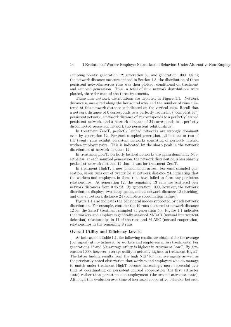
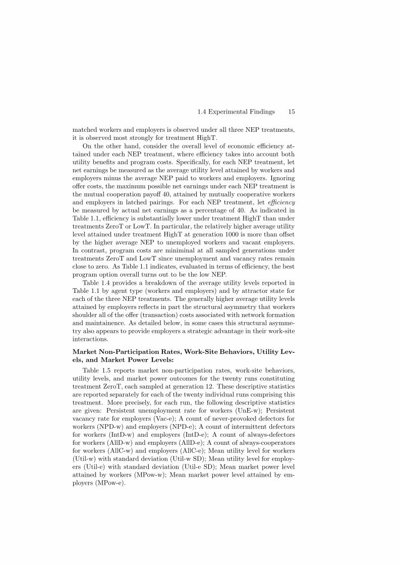
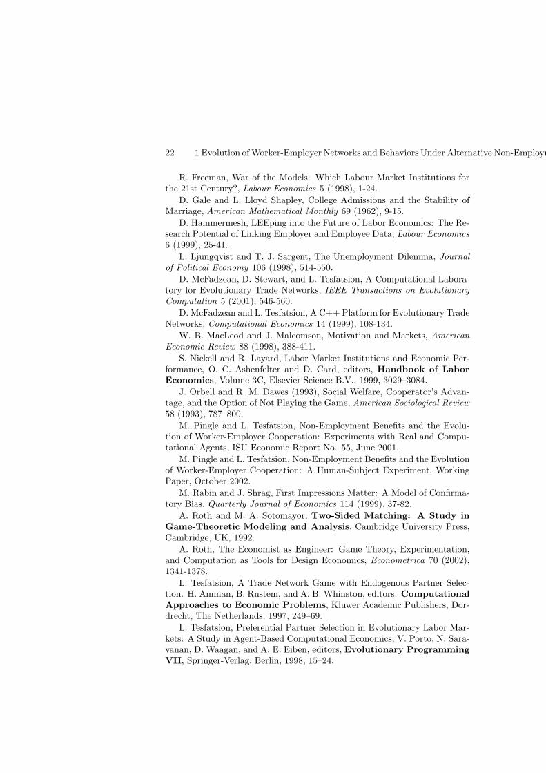
sampling points: generation 12; generation 50; and generation 1000. Usingthe network distance measure defined in Section 1.3, the distribution of thesepersistent networks across runs was then plotted, conditional on treatmentand sampled generation. Thus, a total of nine network distributions wereplotted, three for each of the three treatments.

These nine network distributions are depicted in Figure 1.1. Networkdistance is measured along the horizontal axes and the number of runs clus-tered at this network distance is indicated on the vertical axes. Recall thata network distance of 0 corresponds to a perfectly recurrent (“competitive”)persistent network, a network distance of 12 corresponds to a perfectly latchedpersistent network, and a network distance of 24 corresponds to a perfectlydisconnected persistent network (no persistent relationships).

In treatment ZeroT, perfectly latched networks are strongly dominanteven by generation 12. For each sampled generation, all but one or two ofthe twenty runs exhibit persistent networks consisting of perfectly latchedworker-employer pairs. This is indicated by the sharp peak in the networkdistribution at network distance 12.

In treatment LowT, perfectly latched networks are again dominant. Nev-ertheless, at each sampled generation, the network distribution is less sharplypeaked at network distance 12 than it was for treatment ZeroT.

In treatment HighT, a new phenomenon arises. For each sampled gen-eration, seven runs out of twenty lie at network distance 24, indicating thatthe workers and employers in these runs have failed to form any persistentrelationships. At generation 12, the remaining 13 runs are scattered overnetwork distances from 0 to 23. By generation 1000, however, the networkdistribution displays two sharp peaks, one at network distance 12 (latching)and one at network distance 24 (complete coordination failure).

Figure 1.1 also indicates the behavioral modes supported by each networkdistribution. For example, consider the 19 runs clustered at network distance12 for the ZeroT treatment sampled at generation 50. Figure 1.1 indicatesthat workers and employers generally attained M-IntD (mutual intermittentdefection) relationships in 11 of the runs and M-AllC (mutual cooperation)relationships in the remaining 8 runs.

Overall Utility and Efficiency Levels:

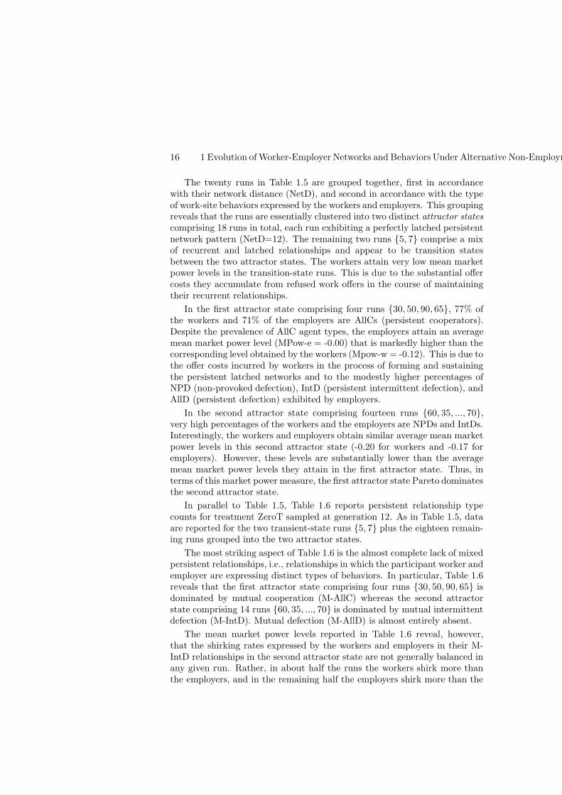
As indicated in Table 1.1, the following results are obtained for the average(per agent) utility achieved by workers and employers across treatments. Forgenerations 12 and 50, average utility is highest in treatment LowT. By gen-eration 1000, however, average utility is actually highest in treatment HighT.The latter finding results from the high NEP for inactive agents as well asthe previously noted observation that workers and employers who do manageto match under treatment HighT become increasingly more successful overtime at coordinating on persistent mutual cooperation (the first attractorstate) rather than persistent non-employment (the second attractor state).Although this evolution over time of increased cooperative behavior between


matched workers and employers is observed under all three NEP treatments,it is observed most strongly for treatment HighT.

On the other hand, consider the overall level of economic efficiency at-tained under each NEP treatment, where efficiency takes into account bothutility benefits and program costs. Specifically, for each NEP treatment, letnet earnings be measured as the average utility level attained by workers andemployers minus the average NEP paid to workers and employers. Ignoringoffer costs, the maximum possible net earnings under each NEP treatment isthe mutual cooperation payoff 40, attained by mutually cooperative workersand employers in latched pairings. For each NEP treatment, let efficiencybe measured by actual net earnings as a percentage of 40. As indicated inTable 1.1, efficiency is substantially lower under treatment HighT than undertreatments ZeroT or LowT. In particular, the relatively higher average utilitylevel attained under treatment HighT at generation 1000 is more than offsetby the higher average NEP to unemployed workers and vacant employers.In contrast, program costs are miniminal at all sampled generations undertreatments ZeroT and LowT since unemployment and vacancy rates remainclose to zero. As Table 1.1 indicates, evaluated in terms of efficiency, the bestprogram option overall turns out to be the low NEP.

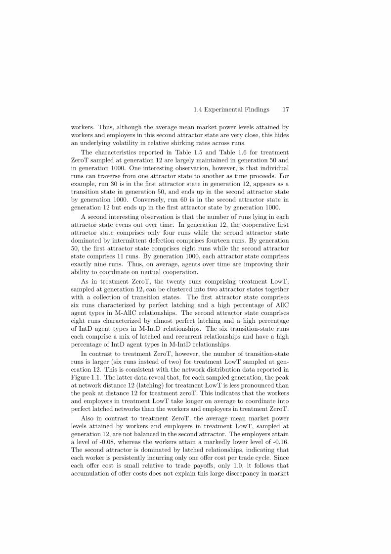
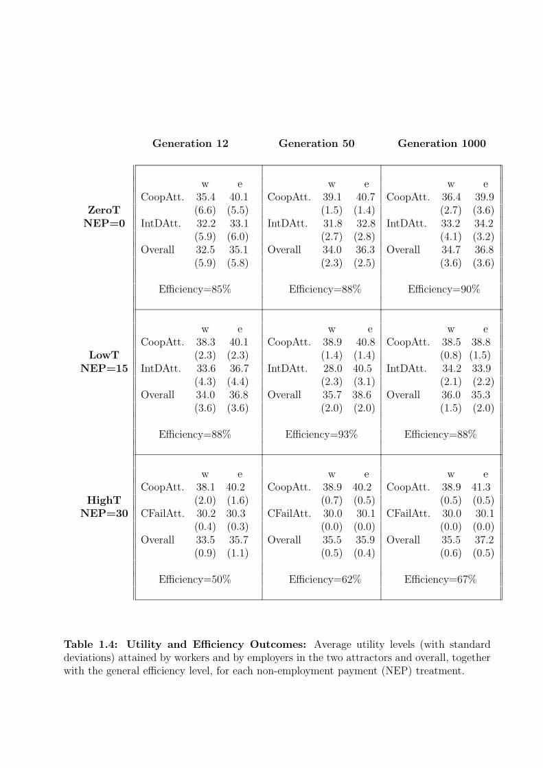
Table 1.4 provides a breakdown of the average utility levels reported inTable 1.1 by agent type (workers and employers) and by attractor state foreach of the three NEP treatments. The generally higher average utility levelsattained by employers reflects in part the structural asymmetry that workersshoulder all of the offer (transaction) costs associated with network formationand maintainence. As detailed below, in some cases this structural asymme-try also appears to provide employers a strategic advantage in their work-siteinteractions.

Market Non-Participation Rates, Work-Site Behaviors, Utility Lev-

els, and Market Power Levels:

Table 1.5 reports market non-participation rates, work-site behaviors,utility levels, and market power outcomes for the twenty runs constitutingtreatment ZeroT, each sampled at generation 12. These descriptive statisticsare reported separately for each of the twenty individual runs comprising thistreatment. More precisely, for each run, the following descriptive statisticsare given: Persistent unemployment rate for workers (UnE-w); Persistentvacancy rate for employers (Vac-e); A count of never-provoked defectors forworkers (NPD-w) and employers (NPD-e); A count of intermittent defectorsfor workers (IntD-w) and employers (IntD-e); A count of always-defectorsfor workers (AllD-w) and employers (AllD-e); A count of always-cooperatorsfor workers (AllC-w) and employers (AllC-e); Mean utility level for workers(Util-w) with standard deviation (Util-w SD); Mean utility level for employ-ers (Util-e) with standard deviation (Util-e SD); Mean market power levelattained by workers (MPow-w); Mean market power level attained by em-ployers (MPow-e).


The twenty runs in Table 1.5 are grouped together, first in accordancewith their network distance (NetD), and second in accordance with the typeof work-site behaviors expressed by the workers and employers. This groupingreveals that the runs are essentially clustered into two distinct attractor statescomprising 18 runs in total, each run exhibiting a perfectly latched persistentnetwork pattern (NetD=12). The remaining two runs {5, 7} comprise a mixof recurrent and latched relationships and appear to be transition statesbetween the two attractor states. The workers attain very low mean marketpower levels in the transition-state runs. This is due to the substantial offercosts they accumulate from refused work offers in the course of maintainingtheir recurrent relationships.

In the first attractor state comprising four runs {30, 50, 90, 65}, 77% ofthe workers and 71% of the employers are AllCs (persistent cooperators).Despite the prevalence of AllC agent types, the employers attain an averagemean market power level (MPow-e = -0.00) that is markedly higher than thecorresponding level obtained by the workers (Mpow-w = -0.12). This is due tothe offer costs incurred by workers in the process of forming and sustainingthe persistent latched networks and to the modestly higher percentages ofNPD (non-provoked defection), IntD (persistent intermittent defection), andAllD (persistent defection) exhibited by employers.

In the second attractor state comprising fourteen runs {60, 35, ..., 70},very high percentages of the workers and the employers are NPDs and IntDs.Interestingly, the workers and employers obtain similar average mean marketpower levels in this second attractor state (-0.20 for workers and -0.17 foremployers). However, these levels are substantially lower than the averagemean market power levels they attain in the first attractor state. Thus, interms of this market power measure, the first attractor state Pareto dominatesthe second attractor state.

In parallel to Table 1.5, Table 1.6 reports persistent relationship typecounts for treatment ZeroT sampled at generation 12. As in Table 1.5, dataare reported for the two transient-state runs {5, 7} plus the eighteen remain-ing runs grouped into the two attractor states.

The most striking aspect of Table 1.6 is the almost complete lack of mixedpersistent relationships, i.e., relationships in which the participant worker andemployer are expressing distinct types of behaviors. In particular, Table 1.6reveals that the first attractor state comprising four runs {30, 50, 90, 65} isdominated by mutual cooperation (M-AllC) whereas the second attractorstate comprising 14 runs {60, 35, ..., 70} is dominated by mutual intermittentdefection (M-IntD). Mutual defection (M-AllD) is almost entirely absent.

The mean market power levels reported in Table 1.6 reveal, however,that the shirking rates expressed by the workers and employers in their M-IntD relationships in the second attractor state are not generally balanced inany given run. Rather, in about half the runs the workers shirk more thanthe employers, and in the remaining half the employers shirk more than the


workers. Thus, although the average mean market power levels attained byworkers and employers in this second attractor state are very close, this hidesan underlying volatility in relative shirking rates across runs.

The characteristics reported in Table 1.5 and Table 1.6 for treatmentZeroT sampled at generation 12 are largely maintained in generation 50 andin generation 1000. One interesting observation, however, is that individualruns can traverse from one attractor state to another as time proceeds. Forexample, run 30 is in the first attractor state in generation 12, appears as atransition state in generation 50, and ends up in the second attractor stateby generation 1000. Conversely, run 60 is in the second attractor state ingeneration 12 but ends up in the first attractor state by generation 1000.

A second interesting observation is that the number of runs lying in eachattractor state evens out over time. In generation 12, the cooperative firstattractor state comprises only four runs while the second attractor statedominated by intermittent defection comprises fourteen runs. By generation50, the first attractor state comprises eight runs while the second attractorstate comprises 11 runs. By generation 1000, each attractor state comprisesexactly nine runs. Thus, on average, agents over time are improving theirability to coordinate on mutual cooperation.

As in treatment ZeroT, the twenty runs comprising treatment LowT,sampled at generation 12, can be clustered into two attractor states togetherwith a collection of transition states. The first attractor state comprisessix runs characterized by perfect latching and a high percentage of AllCagent types in M-AllC relationships. The second attractor state compriseseight runs characterized by almost perfect latching and a high percentageof IntD agent types in M-IntD relationships. The six transition-state runseach comprise a mix of latched and recurrent relationships and have a highpercentage of IntD agent types in M-IntD relationships.

In contrast to treatment ZeroT, however, the number of transition-stateruns is larger (six runs instead of two) for treatment LowT sampled at gen-eration 12. This is consistent with the network distribution data reported inFigure 1.1. The latter data reveal that, for each sampled generation, the peakat network distance 12 (latching) for treatment LowT is less pronounced thanthe peak at distance 12 for treatment zeroT. This indicates that the workersand employers in treatment LowT take longer on average to coordinate intoperfect latched networks than the workers and employers in treatment ZeroT.

Also in contrast to treatment ZeroT, the average mean market powerlevels attained by workers and employers in treatment LowT, sampled atgeneration 12, are not balanced in the second attractor. The employers attaina level of -0.08, whereas the workers attain a markedly lower level of -0.16.The second attractor is dominated by latched relationships, indicating thateach worker is persistently incurring only one offer cost per trade cycle. Sinceeach offer cost is small relative to trade payoffs, only 1.0, it follows thataccumulation of offer costs does not explain this large discrepancy in market


power. Rather, since the second attractor state is dominated by M-IntDrelationships, this discrepancy indicates that the employers are managingto shirk at a substantially higher rate than the workers in these M-IntDrelationships.

The outcomes for treatment LowT sampled at generation 1000 closelyresemble the outcomes reported in Table 1.5 and Table 1.6 for treatmentZeroT sampled at generation 12. The first attractor state comprises nine runsstrongly dominated by M-AllC relationships, and the second attractor statecomprises seven runs strongly dominated by M-IntD relationships. (Hence,an increase in the size of the first attractor state is observed for treatmentLowT in moving from generation 12 to generation 1000.) Mixed types ofrelationships are almost entirely absent in the two attractor states. In thefirst attractor state the workers and employers attain average mean marketpower levels of -0.04 and -0.03, respectively. In the second attractor state theworkers and employers attain uniformly lower but balanced average meanmarket power levels of -0.15. As for treatment ZeroT, this balance hides anunderlying volatility in shirking rates across runs.

Table 1.7 reports market non-participation rates, work-site behaviors,utility levels, and market power outcomes for the twenty runs constitutingtreatment HighT, sampled at generation 12. Table 1.8 reports persistentrelationship type counts for these same runs, again sampled at generation12. As for the previous two treatments, the twenty runs can be clustered intotwo attractor states together with a scattering of transition states. Moreover,once again the runs in the first attractor state exhibit perfectly (or almostperfectly) latched persistent networks with a high percentage of AllC agenttypes. Nevertheless, the nature of the second attractor state is dramaticallydifferent. Whereas in the previous two treatments the second attractor statewas dominated by M-IntD relationships, now the second attractor state corre-sponds to complete or almost complete coordination failure. More precisely,the network distance for the runs in the second attractor state varies from 22(only two persistent relationships) to 24 (no persistent relationships). With ahigh non-employment payment, agents are opting for non-employment ratherthan choosing to remain in M-IntD relationships.

As also seen for treatments ZeroT and LowT, increased coordination onthe first attractor state occurs over time for treatment HighT. In generation12, the first attractor state comprises five runs, the second attractor statecomprises 9 runs, and the six remaining runs are scattered across transitionstates. Also, in the first attractor state, an average of 9.8 out of the 12 persis-tent relationships in each run are M-AllC. By generation 1000, however, thefirst attractor state comprises 11 runs, the second attractor state comprisesseven runs, and only two runs are in a transition state. Moreover, in the firstattractor state, an average of 10.73 out of the 12 persistent relationships ineach run are M-AllC.

Summarizing the relative market power outcomes of workers and employ-


ers in each treatment, the following regularities are observed. For every treat-ment, in each sampled generation, the employers consistently attain a higheraverage market power level than workers in the cooperative first attractorstate. This difference is attributable to the relatively higher (although small)incidence of NPD, IntD, and AllD behaviors among employers and to the factthat offer costs are borne solely by the worker. Also, for treatments ZeroTand HighT, the workers and employers attain essentially the same averagemarket power levels in the second attractor state in each sampled genera-tion; and the same is true for treatment LowT when sampled in generation1000. A balanced market power level in the second attractor state indicateseither that workers and employers have essentially the same shirking rateson average (treatments ZeroT and LowT) or that all agents are persistentlynon-employed (treatment HighT).

With regard to market power in the cooperative first attractor state com-pared across treatments, the workers attain a modestly negative average mar-ket power level in each treatment in each sampled generation; the levels rangefrom -0.12 to -0.02. Interestingly, treatments LowT and HighT have a loweraverage incidence of NPD behavior and a higher average percentage of M-AllC relationships per run than treatment ZeroT in this first attractor state.Nevertheless, these advantages are offset (in market power terms) by thehigher average offer costs incurred by workers due to the longer time takenwithin each generation to establish a persistent network. (For example, asseen in Table 1.7 for treatment HighT sampled at generation 12, only onerun in the first attractor state attains a network distance of 12, i.e., a per-fectly latched persistent network.) In contrast to the workers, employers donot incur offer costs, hence they attain close to a zero average market powerlevel in each treatment at each sampled generation in the cooperative firstattractor state; the levels range from -0.02 to +0.03.

With regard to market power in the second attractor state comparedacross treatments, in each sampled generation both the workers and the em-ployers attain their lowest average levels in treatment HighT. The secondattractor state in treatment HighT is characterized by complete or nearlycomplete coordination failure.

Never-Provoked Defection:

The importance of stance toward strangers and first impressions for de-termining subsequent outcomes in sequential interactions has been stressedby Orbell and Dawes (1993) and by Rabin and Schrag (1999). In the presentcomputational experiment, two sharply differentiated attractor states existfor each treatment, the first dominated by persistent mutual cooperation andthe second dominated either by persistent intermittent defection or by per-sistent non-employment. Thus, outcomes are strongly path dependent, andstance towards strangers and first impressions could play a critical role indetermining these outcomes. These aspects of agent behavior are capturedby counts of never-provoked defection (NPD).


In treatments ZeroT and LowT, NPD is commonly observed in all sam-pled generations, particularly in the second attractor state dominated bypersistent intermittent defection (IntD). For example, as seen in Table 1.5,for treatment ZeroT sampled at generation 12, 33% of workers and 38% ofemployers engage in NPD in the first attractor state, and these percentagesrise to 52% and 83%, respectively, for the second attractor state. It would ap-pear that these high percentages for NPD in the second attractor state mightactually be inducing the resulting predominance of IntD as agents engage inretaliatory defections. Because the non-employment payment is lower thanthe mutual defection payoff in these two treatments, agents tend to defectback against defecting partners rather than simply refusing to interact withthem.

Another interesting observation regarding treatments ZeroT and LowT isthat the incidence of NPD for each agent type in each attractor state tends tobe higher in treatment ZeroT than in treatment LowT. In treatment ZeroT,the non-employment payment 0 lies below all work-site payoffs, including thesucker payoff L=10 earned by an agent who cooperates against a defectingpartner. Consequently, there is no risk of refusal on the basis of bad behavioralone, but only from unfavorable comparisons with other agents. In contrast,in treatment LowT the non-employment payment 15 lies between the suckerpayoff and the mutual defection payoff D=20. In this case, then, an oppor-tunistic agent faces a higher risk of refusal since non-employment is preferredto a sucker payoff.

In treatment HighT the non-employment payment 30 lies above the mu-tual defection payoff for the first time, and the impact of this change in payoffconfiguration is substantial. For example, as reported in Table 5, only 13%of workers and 7% of employers in generation 12 engage in NPD in the firstattractor state characterized by mutual cooperation. In contrast, 100% ofworkers and 97% of employers engage in NPD in the second attractor statecharacterized by complete or almost complete coordination failure. The samepattern holds at generation 50 and generation 1000. Agents are now muchpickier with regard to their partners; an early defection from a partner dropsthat partner’s expected utility assessment below the non-employment payoffand hence below minimum tolerability.

1.5 Concluding Remarks

As detailed by Roth (2002), recent advances in experimental methods andgame theory using both human subjects and computational agents are nowpermitting economists to study a wide variety of complex phenomena associ-ated with decentralized market economies. Examples include inductive pricediscovery, imperfect competition, buyer-seller matching, and the open-endedco-evolution of individual behaviors and economic institutions.

One interesting branch of this literature is the attempt to exploit syner-

1.5 Concluding Remarks 21

gies between experiments with human subjects and experiments with compu-tational agents by means of parallel experimental designs. The few parallelexperimental studies to date have largely focused on financial market issues.9

However, we conjecture that parallel experiments will ultimately prove to beeven more valuable when applied to economic processes such as labor marketsin which face-to-face personal relationships play a potentially strong role indetermining market outcomes.

The preliminary ACE labor market study at hand highlights the need tocarefully align parallel experimental designs to ensure valid comparability.For example, transaction costs must be properly scaled across experimentsto ensure comparable agent incentives, and horizons need to be aligned toensure that short-run and long-run effects are properly distinguished.

In future ACE labor market studies, we intend to calibrate our parallel ex-perimental designs to empirical data. Salient aspects of actual unemploymentbenefit programs will be incorporated, and findings from previous empiricalstudies of unemployment benefit programs will be used wherever possible.In addition, the recent construction of linked employer-employee (LEE) datasets is an exciting development facilitating the empirical study of outcomesgenerated by worker-employer interactions; see Hammermesh (1999). LEEdata sets complement beautifully the focus of ACE labor market studies onworker-employer interaction patterns. Consequently, LEE data should per-mit careful empirical testing of computational findings related specificallyto interaction effects, such as strong path dependence and the existence ofmultiple attractors.

Acknowledgments

The authors are grateful for helpful comments received from an anonymousreferee, from Peter Orazem, from Marshall Van Alstyne and other partici-pants in the UCLA Computational Social Sciences Conference held in May2002 at Lake Arrowhead, California, and from Richard Freeman and otherparticipants in the Harvard University Colloquium on Complexity and SocialNetworks held on April 7, 2003.

References

D. Acemoglu and R. Shimer, Productivity Gains from UnemploymentInsurance, European Economic Review 44 (2000), 1195-1223.

F. D. Blau and L. M. Kahn, Institutional Differences in Male Wage In-equality: Institutions versus Market Forces, O. Ashenfelter and D. Card,editors, Handbook of Labor Economics, Volume 3A, Elsevier ScienceB.V., 1999, 1399–1461.

9See http://www.econ.iastate.edu/tesfatsi/aexper.htm for pointers to research usingparallel experiments.


R. Freeman, War of the Models: Which Labour Market Institutions forthe 21st Century?, Labour Economics 5 (1998), 1-24.

D. Gale and L. Lloyd Shapley, College Admissions and the Stability ofMarriage, American Mathematical Monthly 69 (1962), 9-15.

D. Hammermesh, LEEping into the Future of Labor Economics: The Re-search Potential of Linking Employer and Employee Data, Labour Economics6 (1999), 25-41.

L. Ljungqvist and T. J. Sargent, The Unemployment Dilemma, Journalof Political Economy 106 (1998), 514-550.

D. McFadzean, D. Stewart, and L. Tesfatsion, A Computational Labora-tory for Evolutionary Trade Networks, IEEE Transactions on EvolutionaryComputation 5 (2001), 546-560.

D. McFadzean and L. Tesfatsion, A C++ Platform for Evolutionary TradeNetworks, Computational Economics 14 (1999), 108-134.

W. B. MacLeod and J. Malcomson, Motivation and Markets, AmericanEconomic Review 88 (1998), 388-411.

S. Nickell and R. Layard, Labor Market Institutions and Economic Per-formance, O. C. Ashenfelter and D. Card, editors, Handbook of Labor

Economics, Volume 3C, Elsevier Science B.V., 1999, 3029–3084.

J. Orbell and R. M. Dawes (1993), Social Welfare, Cooperator’s Advan-tage, and the Option of Not Playing the Game, American Sociological Review58 (1993), 787–800.

M. Pingle and L. Tesfatsion, Non-Employment Benefits and the Evolu-tion of Worker-Employer Cooperation: Experiments with Real and Compu-tational Agents, ISU Economic Report No. 55, June 2001.

M. Pingle and L. Tesfatsion, Non-Employment Benefits and the Evolutionof Worker-Employer Cooperation: A Human-Subject Experiment, WorkingPaper, October 2002.

M. Rabin and J. Shrag, First Impressions Matter: A Model of Confirma-tory Bias, Quarterly Journal of Economics 114 (1999), 37-82.

A. Roth and M. A. Sotomayor, Two-Sided Matching: A Study in

Game-Theoretic Modeling and Analysis, Cambridge University Press,Cambridge, UK, 1992.

A. Roth, The Economist as Engineer: Game Theory, Experimentation,and Computation as Tools for Design Economics, Econometrica 70 (2002),1341-1378.

L. Tesfatsion, A Trade Network Game with Endogenous Partner Selec-tion. H. Amman, B. Rustem, and A. B. Whinston, editors. Computational

Approaches to Economic Problems, Kluwer Academic Publishers, Dor-drecht, The Netherlands, 1997, 249–69.

L. Tesfatsion, Preferential Partner Selection in Evolutionary Labor Mar-kets: A Study in Agent-Based Computational Economics, V. Porto, N. Sara-vanan, D. Waagan, and A. E. Eiben, editors, Evolutionary Programming

VII, Springer-Verlag, Berlin, 1998, 15–24.

1.5 Concluding Remarks 23

L. Tesfatsion, Structure, Behavior and Market power in an EvolutionaryLabor Market with Adaptive Search, Journal of Economic Dynamics andControl 25 (2001), 419–457.

L. Tesfatsion, Hysteresis in an Evolutionary Labor Market with AdaptiveSearch, S.-H. Chen, editor, Evolutionary Computation in Economics

and Finance, Physica-Verlag Heidelberg, 2002a, 189–210.L. Tesfatsion, Economic Agents and Markets as Emergent Phenomena,

Proceedings of the National Academy of Sciences U.S.A., Volume 99, Supple-ment 3 (2002b), 7191–7192.

L. Tesfatsion, Agent-Based Computational Economics, Francesco Luna,Alessandro Perrone, and Pietro Terna, editors, Agent-Based Theories,

Languages, and Practices, Routledge Publishers, 2003, to appear.

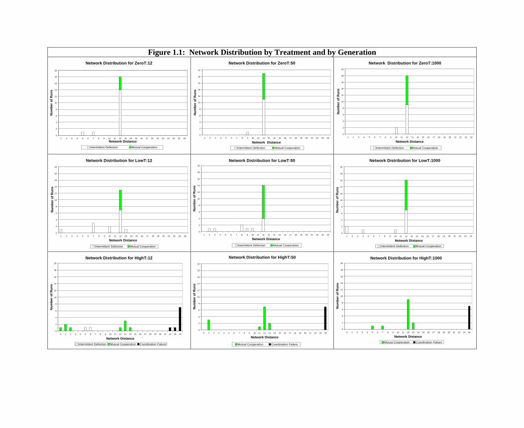
Figure 1.1: Network Distribution by Treatment and by GenerationNetwork Distribution for ZeroT:12

0

2

4

6

8

10

12

14

16

18

20

1 2 3 4 5 6 7 8 9 10 11 12 13 14 15 16 17 18 19 20 21 22 23 24

Network Distance

Nu

mb

er o

f R

un

s

Intermittent Defection Mutual Cooperation

Network Distribution for ZeroT:50

0

2

4

6

8

10

12

14

16

18

20

1 2 3 4 5 6 7 8 9 10 11 12 13 14 15 16 17 18 19 20 21 22 23 24

Network Distance

Nu

mb

er o

f R

un

s


Network Distribution for ZeroT:1000

0

2

4

6

8

10

12

14

16

18

20

1 2 3 4 5 6 7 8 9 10 11 12 13 14 15 16 17 18 19 20 21 22 23 24

Network Distance

Nu

mb

er o

f R

un

s

Intermittant Defection Mutual Cooperation

Network Distribution for LowT:12

0

2

4

6

8

10

12

14

16

18

20

1 2 3 4 5 6 7 8 9 10 11 12 13 14 15 16 17 18 19 20 21 22 23 24

Network Distance

Nu

mb

er o

f R

un

s



0

2

4

6

8

10

12

14

16

18

20

1 2 3 4 5 6 7 8 9 10 11 12 13 14 15 16 17 18 19 20 21 22 23 24

Network Distance

Nu

mb

er o

f R

un

s



0

2

4

6

8

10

12

14

16

18

20

1 2 3 4 5 6 7 8 9 10 11 12 13 14 15 16 17 18 19 20 21 22 23 24

Network Distance

Nu

mb

er o

f R

un

s


Network Distribution for HighT:12

0

2

4

6

8

10

12

14

16

18

20

0 1 2 3 4 5 6 7 8 9 10 11 12 13 14 15 16 17 18 19 20 21 22 23 24

Network Distance

Nu

mb

er o

f R

un

s

Intermittent Defection Mutual Cooperation Coordination Failure


0

2

4

6

8

10

12

14

16

18

20

0 1 2 3 4 5 6 7 8 9 10 11 12 13 14 15 16 17 18 19 20 21 22 23 24

Network Distance

Nu

mb

er o

f R

un

s

Mutual Cooperation Coordination Failure


0

2

4

6

8

10

12

14

16

18

20

0 1 2 3 4 5 6 7 8 9 10 11 12 13 14 15 16 17 18 19 20 21 22 23 24

Network DistanceN

um

ber

of

Ru

ns

Mutual Cooperation Coordination Failure

Generation 12 Generation 50 Generation 1000

Utility 33.8 (5.9) Utility 35.2 (2.8) Utility 35.8 (3.6)ZeroT Unemp 0% UnEmp 0% UnEmp 0%

NEP=0 Vacancy 0% Vacancy 0% Vacancy 0%Efficiency 85% Efficiency 88% Efficiency 90%

Utility 35.4 (3.6) Utility 37.2 (2.0) Utility 35.7 (1.8)LowT UnEmp 1% UnEmp 0% UnEmp 2%


Utility 34.6 (1.0) Utility 35.7 (0.5) Utility 36.4 (0.6)HighT Unemp 48% Unemp 36% UnEmp 32%


Table 1.1: Summary of Aggregate Outcomes: Average agent utility level (with stan-dard deviation), worker unemployment rate, employer vacancy rate, and efficiency level foreach non-employment payment (NEP) treatment.

int main () {

InitiateEconomy(); // CONSTRUCT initial subpopulations of// workers and employers with random// work-site rules of behavior.

For (G = 1,...,1000) { // ENTER THE GENERATION CYCLE LOOP

// GENERATION CYCLE:

InitiateGen(); // Configure workers and employers// with user-supplied parameter values// (initial expected utility assessments,// minimum tolerance levels,...)

For (TC = 1,...,150) { // ENTER THE TRADE CYCLE LOOP

// TRADE CYCLE:

MatchTraders(); // Workers and employers determine// their work-site partners, given// their expected utility assessments,// and record job search and// inactivity costs.

Trade(); // Workers and employers engage// in work-site interactions and// record their work-site payoffs.

UpdateExp(); // Workers and employers update their// expected utility assessments, using// newly recorded costs and work-site// payoffs, and begin a new trade cycle.

}// ENVIRONMENT STEP:

AssessFitness(); // Each worker and employer assesses// his utility (fitness) level.

// EVOLUTION STEP:

EvolveGen(); // Workers and employers separately// evolve their work-site rules,// and a new generation cycle begins.

}Return 0;

}

Table 1.2: Flow of Activities in the ACE Labor Market

Employerc d

c (40,40) (10,60)Worker

d (60,10) (20,20)

Table 1.3: Payoff Matrix for the Work-Site Prisoner’s Dilemma Game

Generation 12 Generation 50 Generation 1000

w e w e w eCoopAtt. 35.4 40.1 CoopAtt. 39.1 40.7 CoopAtt. 36.4 39.9

ZeroT (6.6) (5.5) (1.5) (1.4) (2.7) (3.6)NEP=0 IntDAtt. 32.2 33.1 IntDAtt. 31.8 32.8 IntDAtt. 33.2 34.2

(5.9) (6.0) (2.7) (2.8) (4.1) (3.2)Overall 32.5 35.1 Overall 34.0 36.3 Overall 34.7 36.8

(5.9) (5.8) (2.3) (2.5) (3.6) (3.6)

Efficiency=85% Efficiency=88% Efficiency=90%


LowT (2.3) (2.3) (1.4) (1.4) (0.8) (1.5)NEP=15 IntDAtt. 33.6 36.7 IntDAtt. 28.0 40.5 IntDAtt. 34.2 33.9


(3.6) (3.6) (2.0) (2.0) (1.5) (2.0)



HighT (2.0) (1.6) (0.7) (0.5) (0.5) (0.5)NEP=30 CFailAtt. 30.2 30.3 CFailAtt. 30.0 30.1 CFailAtt. 30.0 30.1


(0.9) (1.1) (0.5) (0.4) (0.6) (0.5)


Table 1.4: Utility and Efficiency Outcomes: Average utility levels (with standarddeviations) attained by workers and by employers in the two attractors and overall, togetherwith the general efficiency level, for each non-employment payment (NEP) treatment.

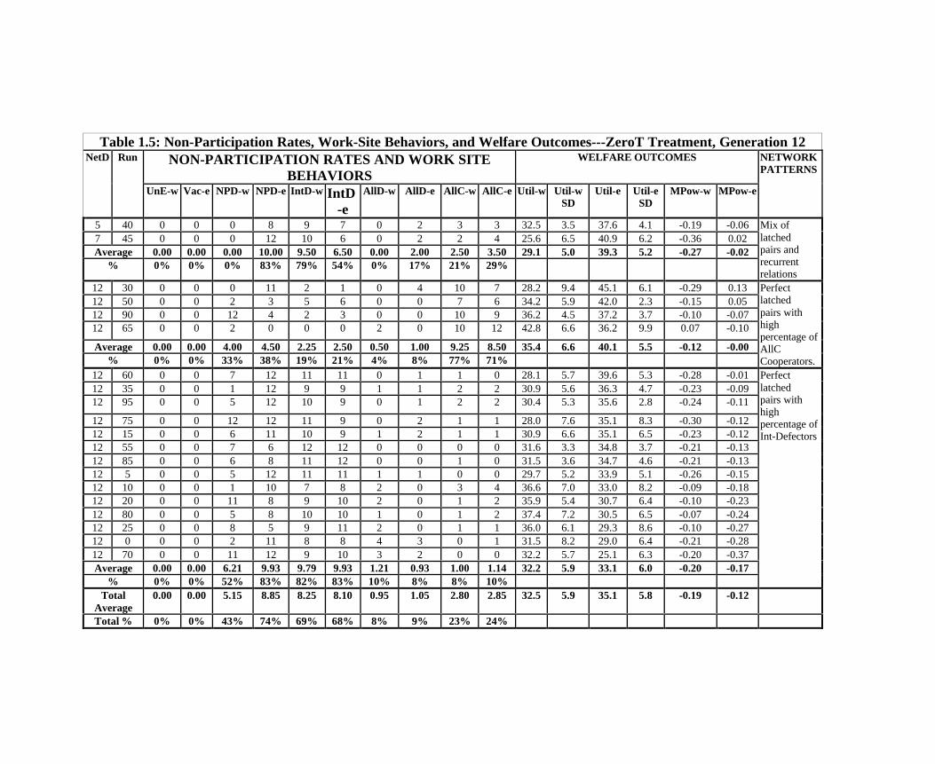
Table 1.5: Non-Participation Rates, Work-Site Behaviors, and Welfare Outcomes---ZeroT Treatment, Generation 12NON-PARTICIPATION RATES AND WORK SITE

BEHAVIORSWELFARE OUTCOMESNetD Run

UnE-w Vac-e NPD-w NPD-e IntD-w IntD-e

AllD-w AllD-e AllC-w AllC-e Util-w Util-wSD

Util-e Util-eSD

MPow-w MPow-e

NETWORKPATTERNS

5 40 0 0 0 8 9 7 0 2 3 3 32.5 3.5 37.6 4.1 -0.19 -0.067 45 0 0 0 12 10 6 0 2 2 4 25.6 6.5 40.9 6.2 -0.36 0.02Average 0.00 0.00 0.00 10.00 9.50 6.50 0.00 2.00 2.50 3.50 29.1 5.0 39.3 5.2 -0.27 -0.02

% 0% 0% 0% 83% 79% 54% 0% 17% 21% 29%

Mix oflatchedpairs andrecurrentrelations

12 30 0 0 0 11 2 1 0 4 10 7 28.2 9.4 45.1 6.1 -0.29 0.1312 50 0 0 2 3 5 6 0 0 7 6 34.2 5.9 42.0 2.3 -0.15 0.0512 90 0 0 12 4 2 3 0 0 10 9 36.2 4.5 37.2 3.7 -0.10 -0.0712 65 0 0 2 0 0 0 2 0 10 12 42.8 6.6 36.2 9.9 0.07 -0.10

Average 0.00 0.00 4.00 4.50 2.25 2.50 0.50 1.00 9.25 8.50 35.4 6.6 40.1 5.5 -0.12 -0.00% 0% 0% 33% 38% 19% 21% 4% 8% 77% 71%

Perfectlatchedpairs withhighpercentage ofAllCCooperators.

12 60 0 0 7 12 11 11 0 1 1 0 28.1 5.7 39.6 5.3 -0.28 -0.0112 35 0 0 1 12 9 9 1 1 2 2 30.9 5.6 36.3 4.7 -0.23 -0.0912 95 0 0 5 12 10 9 0 1 2 2 30.4 5.3 35.6 2.8 -0.24 -0.11

12 75 0 0 12 12 11 9 0 2 1 1 28.0 7.6 35.1 8.3 -0.30 -0.1212 15 0 0 6 11 10 9 1 2 1 1 30.9 6.6 35.1 6.5 -0.23 -0.1212 55 0 0 7 6 12 12 0 0 0 0 31.6 3.3 34.8 3.7 -0.21 -0.1312 85 0 0 6 8 11 12 0 0 1 0 31.5 3.6 34.7 4.6 -0.21 -0.1312 5 0 0 5 12 11 11 1 1 0 0 29.7 5.2 33.9 5.1 -0.26 -0.1512 10 0 0 1 10 7 8 2 0 3 4 36.6 7.0 33.0 8.2 -0.09 -0.1812 20 0 0 11 8 9 10 2 0 1 2 35.9 5.4 30.7 6.4 -0.10 -0.2312 80 0 0 5 8 10 10 1 0 1 2 37.4 7.2 30.5 6.5 -0.07 -0.2412 25 0 0 8 5 9 11 2 0 1 1 36.0 6.1 29.3 8.6 -0.10 -0.2712 0 0 0 2 11 8 8 4 3 0 1 31.5 8.2 29.0 6.4 -0.21 -0.2812 70 0 0 11 12 9 10 3 2 0 0 32.2 5.7 25.1 6.3 -0.20 -0.37Average 0.00 0.00 6.21 9.93 9.79 9.93 1.21 0.93 1.00 1.14 32.2 5.9 33.1 6.0 -0.20 -0.17

% 0% 0% 52% 83% 82% 83% 10% 8% 8% 10%

Perfectlatchedpairs withhighpercentage ofInt-Defectors

TotalAverage

0.00 0.00 5.15 8.85 8.25 8.10 0.95 1.05 2.80 2.85 32.5 5.9 35.1 5.8 -0.19 -0.12

Total % 0% 0% 43% 74% 69% 68% 8% 9% 23% 24%

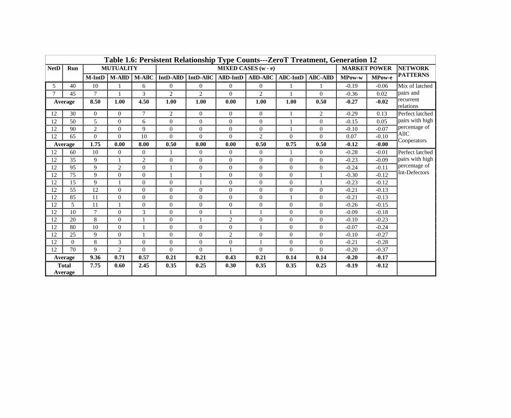
Table 1.6: Persistent Relationship Type Counts---ZeroT Treatment, Generation 12MUTUALITY MIXED CASES (w - e) MARKET POWERNetD Run

M-IntD M-AllD M-AllC IntD-AllD IntD-AllC AllD-IntD AllD-AllC AllC-IntD AllC-AllD MPow-w MPow-e

NETWORKPATTERNS

5 40 10 1 6 0 0 0 0 1 1 -0.19 -0.067 45 7 1 3 2 2 0 2 1 0 -0.36 0.02Average 8.50 1.00 4.50 1.00 1.00 0.00 1.00 1.00 0.50 -0.27 -0.02

Mix of latchedpairs andrecurrentrelations

12 30 0 0 7 2 0 0 0 1 2 -0.29 0.1312 50 5 0 6 0 0 0 0 1 0 -0.15 0.0512 90 2 0 9 0 0 0 0 1 0 -0.10 -0.0712 65 0 0 10 0 0 0 2 0 0 0.07 -0.10Average 1.75 0.00 8.00 0.50 0.00 0.00 0.50 0.75 0.50 -0.12 -0.00

Perfect latchedpairs with highpercentage ofAllCCooperators

12 60 10 0 0 1 0 0 0 1 0 -0.28 -0.0112 35 9 1 2 0 0 0 0 0 0 -0.23 -0.0912 95 9 2 0 1 0 0 0 0 0 -0.24 -0.1112 75 9 0 0 1 1 0 0 0 1 -0.30 -0.1212 15 9 1 0 0 1 0 0 0 1 -0.23 -0.1212 55 12 0 0 0 0 0 0 0 0 -0.21 -0.1312 85 11 0 0 0 0 0 0 1 0 -0.21 -0.1312 5 11 1 0 0 0 0 0 0 0 -0.26 -0.1512 10 7 0 3 0 0 1 1 0 0 -0.09 -0.1812 20 8 0 1 0 1 2 0 0 0 -0.10 -0.2312 80 10 0 1 0 0 0 1 0 0 -0.07 -0.2412 25 9 0 1 0 0 2 0 0 0 -0.10 -0.2712 0 8 3 0 0 0 0 1 0 0 -0.21 -0.2812 70 9 2 0 0 0 1 0 0 0 -0.20 -0.37Average 9.36 0.71 0.57 0.21 0.21 0.43 0.21 0.14 0.14 -0.20 -0.17

Perfect latchedpairs with highpercentage ofInt-Defectors

TotalAverage

7.75 0.60 2.45 0.35 0.25 0.30 0.35 0.35 0.25 -0.19 -0.12

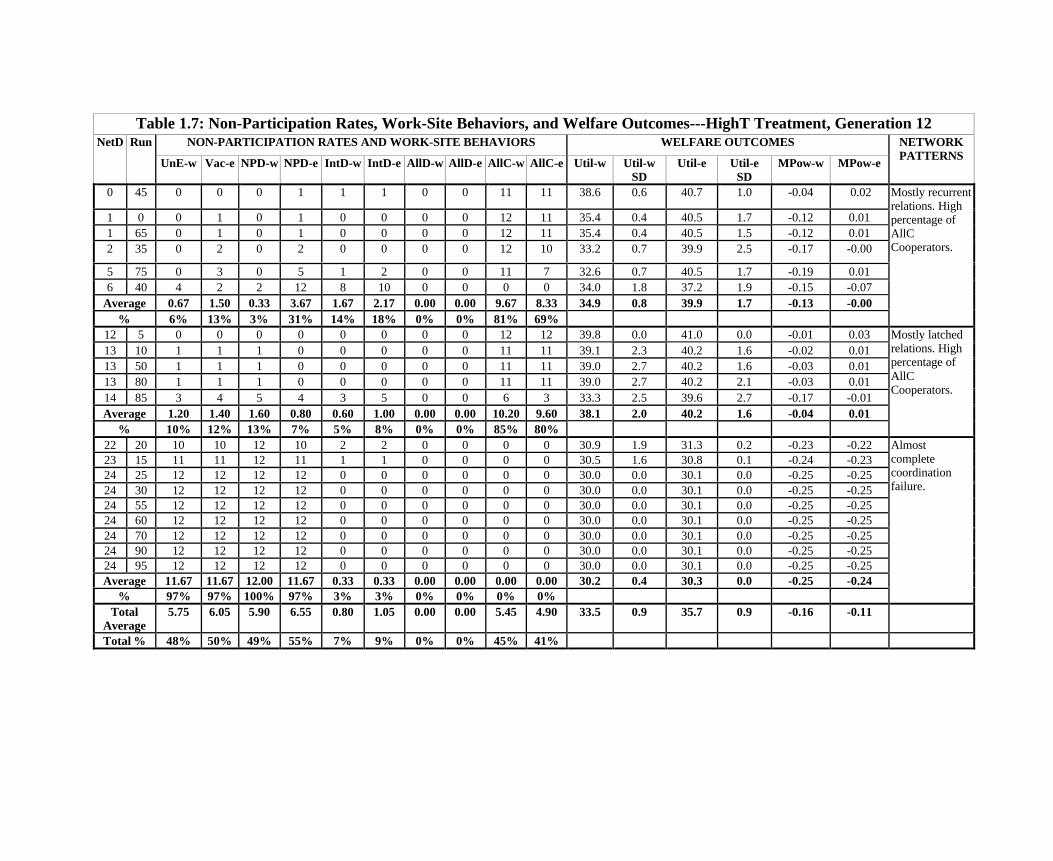
Table 1.7: Non-Participation Rates, Work-Site Behaviors, and Welfare Outcomes---HighT Treatment, Generation 12NON-PARTICIPATION RATES AND WORK-SITE BEHAVIORS WELFARE OUTCOMESNetD Run

UnE-w Vac-e NPD-w NPD-e IntD-w IntD-e AllD-w AllD-e AllC-w AllC-e Util-w Util-wSD

Util-e Util-eSD

MPow-w MPow-e

NETWORKPATTERNS

0 45 0 0 0 1 1 1 0 0 11 11 38.6 0.6 40.7 1.0 -0.04 0.02

1 0 0 1 0 1 0 0 0 0 12 11 35.4 0.4 40.5 1.7 -0.12 0.011 65 0 1 0 1 0 0 0 0 12 11 35.4 0.4 40.5 1.5 -0.12 0.012 35 0 2 0 2 0 0 0 0 12 10 33.2 0.7 39.9 2.5 -0.17 -0.00

5 75 0 3 0 5 1 2 0 0 11 7 32.6 0.7 40.5 1.7 -0.19 0.016 40 4 2 2 12 8 10 0 0 0 0 34.0 1.8 37.2 1.9 -0.15 -0.07

Average 0.67 1.50 0.33 3.67 1.67 2.17 0.00 0.00 9.67 8.33 34.9 0.8 39.9 1.7 -0.13 -0.00% 6% 13% 3% 31% 14% 18% 0% 0% 81% 69%

Mostly recurrentrelations. Highpercentage ofAllCCooperators.

12 5 0 0 0 0 0 0 0 0 12 12 39.8 0.0 41.0 0.0 -0.01 0.0313 10 1 1 1 0 0 0 0 0 11 11 39.1 2.3 40.2 1.6 -0.02 0.0113 50 1 1 1 0 0 0 0 0 11 11 39.0 2.7 40.2 1.6 -0.03 0.0113 80 1 1 1 0 0 0 0 0 11 11 39.0 2.7 40.2 2.1 -0.03 0.0114 85 3 4 5 4 3 5 0 0 6 3 33.3 2.5 39.6 2.7 -0.17 -0.01Average 1.20 1.40 1.60 0.80 0.60 1.00 0.00 0.00 10.20 9.60 38.1 2.0 40.2 1.6 -0.04 0.01

% 10% 12% 13% 7% 5% 8% 0% 0% 85% 80%

Mostly latchedrelations. Highpercentage ofAllCCooperators.

22 20 10 10 12 10 2 2 0 0 0 0 30.9 1.9 31.3 0.2 -0.23 -0.2223 15 11 11 12 11 1 1 0 0 0 0 30.5 1.6 30.8 0.1 -0.24 -0.2324 25 12 12 12 12 0 0 0 0 0 0 30.0 0.0 30.1 0.0 -0.25 -0.2524 30 12 12 12 12 0 0 0 0 0 0 30.0 0.0 30.1 0.0 -0.25 -0.2524 55 12 12 12 12 0 0 0 0 0 0 30.0 0.0 30.1 0.0 -0.25 -0.2524 60 12 12 12 12 0 0 0 0 0 0 30.0 0.0 30.1 0.0 -0.25 -0.2524 70 12 12 12 12 0 0 0 0 0 0 30.0 0.0 30.1 0.0 -0.25 -0.2524 90 12 12 12 12 0 0 0 0 0 0 30.0 0.0 30.1 0.0 -0.25 -0.2524 95 12 12 12 12 0 0 0 0 0 0 30.0 0.0 30.1 0.0 -0.25 -0.25Average 11.67 11.67 12.00 11.67 0.33 0.33 0.00 0.00 0.00 0.00 30.2 0.4 30.3 0.0 -0.25 -0.24

% 97% 97% 100% 97% 3% 3% 0% 0% 0% 0%

Almostcompletecoordinationfailure.

TotalAverage

5.75 6.05 5.90 6.55 0.80 1.05 0.00 0.00 5.45 4.90 33.5 0.9 35.7 0.9 -0.16 -0.11

Total % 48% 50% 49% 55% 7% 9% 0% 0% 45% 41%

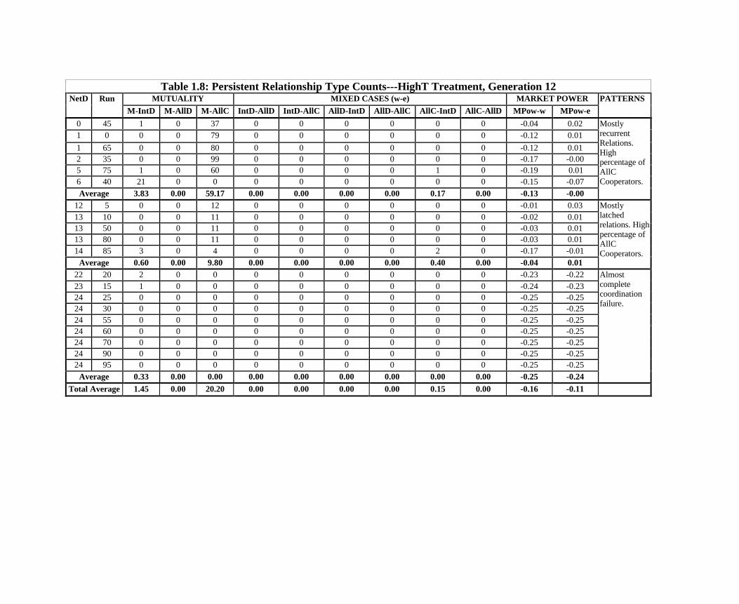
Table 1.8: Persistent Relationship Type Counts---HighT Treatment, Generation 12MUTUALITY MIXED CASES (w-e) MARKET POWERNetD Run

M-IntD M-AllD M-AllC IntD-AllD IntD-AllC AllD-IntD AllD-AllC AllC-IntD AllC-AllD MPow-w MPow-ePATTERNS

0 45 1 0 37 0 0 0 0 0 0 -0.04 0.021 0 0 0 79 0 0 0 0 0 0 -0.12 0.011 65 0 0 80 0 0 0 0 0 0 -0.12 0.012 35 0 0 99 0 0 0 0 0 0 -0.17 -0.005 75 1 0 60 0 0 0 0 1 0 -0.19 0.016 40 21 0 0 0 0 0 0 0 0 -0.15 -0.07Average 3.83 0.00 59.17 0.00 0.00 0.00 0.00 0.17 0.00 -0.13 -0.00

MostlyrecurrentRelations.Highpercentage ofAllCCooperators.

12 5 0 0 12 0 0 0 0 0 0 -0.01 0.0313 10 0 0 11 0 0 0 0 0 0 -0.02 0.0113 50 0 0 11 0 0 0 0 0 0 -0.03 0.0113 80 0 0 11 0 0 0 0 0 0 -0.03 0.0114 85 3 0 4 0 0 0 0 2 0 -0.17 -0.01

Average 0.60 0.00 9.80 0.00 0.00 0.00 0.00 0.40 0.00 -0.04 0.01

Mostlylatchedrelations. Highpercentage ofAllCCooperators.

22 20 2 0 0 0 0 0 0 0 0 -0.23 -0.2223 15 1 0 0 0 0 0 0 0 0 -0.24 -0.2324 25 0 0 0 0 0 0 0 0 0 -0.25 -0.2524 30 0 0 0 0 0 0 0 0 0 -0.25 -0.2524 55 0 0 0 0 0 0 0 0 0 -0.25 -0.2524 60 0 0 0 0 0 0 0 0 0 -0.25 -0.2524 70 0 0 0 0 0 0 0 0 0 -0.25 -0.2524 90 0 0 0 0 0 0 0 0 0 -0.25 -0.2524 95 0 0 0 0 0 0 0 0 0 -0.25 -0.25

Average 0.33 0.00 0.00 0.00 0.00 0.00 0.00 0.00 0.00 -0.25 -0.24

Almostcompletecoordinationfailure.

Total Average 1.45 0.00 20.20 0.00 0.00 0.00 0.00 0.15 0.00 -0.16 -0.11

Documents

Contribution for Innovations in Financial and Economic ... · Contribution for Innovations in Financial and Economic Networks Anna Nagurney, editor ... Department of Economics Iowa