CONTROL SYSTEM

LAB MANUAL

EIC 551

DEPARTMENT OF ELECTRONICS AND COMMUNICATION ENGINEERING

27, Knowledge Park-III, Greater Noida, (U.P.) Phone : 0120-2322022

website :- www.dronacharya.info

EXPERIMENT NO. 1

OBJECTIVE: DC MOTOR POSITION CONTROL

(A) TO STUDY OF POTENTIONMETER DISPLACEMENT CONSTANT THROUGH CONTINUOUS COMMAND.

(B) TO STUDY OF DC POSITION CONTROL THROUGH CONTINUOUS COMMAND. (C) TO STUDY OF DC POSITION CONTROL THROUGH STEP COMMAND. (D) TO STUDY OF DC POSITION CONTROL THROUGH DYNAMIC RESPONSE.

APPARATUS REQUIRED:

S. No. Name of the Equipment Used Specification Quantity

1. DC Position control system kit

2. CRO

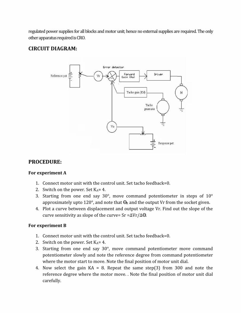
THEORY: A DC position control system is a closed loop control system in which

the position of the mechanical load is controlled with the position of the reference shaft. A pair of

potentiometers acts as error-measuring device. They convert the input and output positions

into proportional electric signals. The desired position is set on the input potentiometer and the actual

position is fed to feedback potentiometer. The difference between the two angular positions

generates an e r r o r s i g n a l , w h i c h i s a m p l i f i e d a n d f e d t o a r m a t u r e c i r c u i t

o f t h e D C m o t o r . T h e tacho-generator attached to the motor shaft produces a voltage

proportional to the speed which is used for feedback. If an error exists, the motor develops a torque to

rotate the output in such a way as to reduce the error to zero .The rotation of the motor stops

when the error signal is zero, i.e., when the desired position is reached.

The setup of DC position control system is designed to study dc motor position control system called

servomechanism and comes first in automatic control systems. The prime advantage of this setup is near

perfection to this simulated system. The set up comprises of two parts:-

(a.) The motor unit

(b.) The control unit

The motor unit:-It consists a permanent magnet armature controlled geared servo motor servo motor. It

has technical specifications as operating voltage: 12 Vdc , 5W. Rated shaft speed 50RPM. Torque: 3.5Kg/cm

at load shaft. The angular displacement is sensed by a 360° servo potentiometer. A graduated disc is

mounted upon the potentiometer to indicate angular position with 1° resolution.

The control unit: -This unit has reference servo potentiometer, voltage source, error detector, amplifier,

motor drive circuit, and a RAM card necessary regulated supplies for the circuits. The unit has built in dc

regulated power supplies for all blocks and motor unit; hence no external supplies are required. The only

other apparatus required is CRO.

CIRCUIT DIAGRAM:

PROCEDURE:

For experiment A

1. Connect motor unit with the control unit. Set tacho feedback=0.

2. Switch on the power. Set KA= 4.

3. Starting from one end say 30°, move command potentiometer in steps of 10°

approximately upto 120°, and note that ϴR and the output Vr from the socket given.

4. Plot a curve between displacement and output voltage Vr. Find out the slope of the

curve sensitivity as slope of the curve= Sr =∆Vr/∆ϴ.

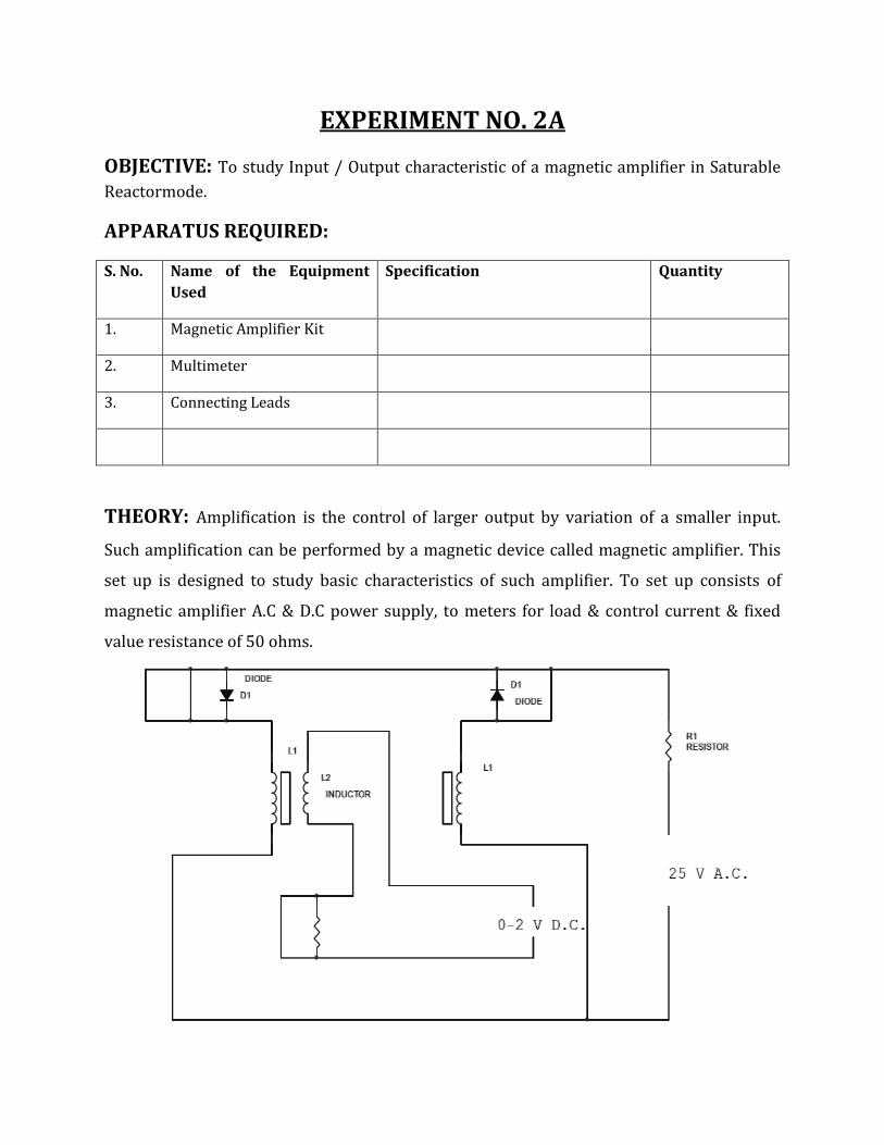
For experiment B

1. Connect motor unit with the control unit. Set tacho feedback=0.

2. Switch on the power. Set KA= 4.

3. Starting from one end say 30°, move command potentiometer move command

potentiometer slowly and note the reference degree from command potentiometer

where the motor start to move. Note the final position of motor unit dial.

4. Now select the gain KA = 8. Repeat the same step(3) from 300 and note the

reference degree where the motor move. . Note the final position of motor unit dial

carefully.

5. From these observations it is shown that when the gain constant is low the motor

position does not follow quickly the command signal which means there is great ess.

When gain is set to 8 or 9, the follow of motor is earlier than previous and motor

exhibit oscillation but there is a small state error.

For experiment C

1. Set KA= 3. Keep tacho feedback at 0. Command dial at 90°. Connect given voltmeter

with Vr socket and note the voltage there as Vr.

2. Connect voltmeter across V0 socket. Note the voltage reading as Vol.

3. Connect voltmeter at VS socket and apply step input by briefly push upon step key.

Note the dc steady state voltage there after time lapse of 11 second the motor will

be back to its previous position.

4. Connect the voltmeter with Vo socket and reapply the step signal. Note the reading

of Vo as Vo2.

5. Calculate the step change as V1 = (Vr+Vs) and find out the ess as ess = (V1-Vo) where

feedback voltage Vo= Vo2-Vo1.

6. Now set KA = 8. The voltmeter is still connected with Vo socket. Apply the step signal

and note the steady state voltage Vo2 and Vo1. Find out the ess.

7. From this experiment it is observed that motor does not follow a sudden change in

position command when the gain of control amplifier is low, which verify by the ess

rate. It is verified in next experiment.

For experiment D

1. Select KA=3. Keep command potentiometer at 90º. Connect CRO at X-Y output

sockets with reference to ground in X-Y mode. Set Y at 0.2V/div and X at 0.5V/div.

2. Press capture key briefly, a spot will appear upon screen. Press step key briefly, the

motor will be run. Wait till capture time is complete. After completion of capture

time the captured waveform will be displayed upon the screen.

3. Connect given DVM at VO and note the voltage as initial. Apply step signal and note

the voltage at new position.

4. Trace the waveform.

5. Increase the gain to 5, 7, 9 and each time capture a new waveform trace it upon

paper with CRO graticule as reference.

6. Select the wave form look like second order response curve.

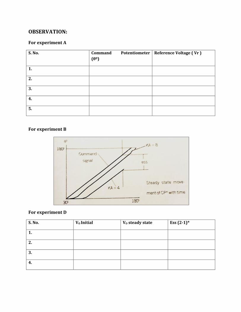
OBSERVATION:

For experiment A

S. No. Command Potentiometer

(θº)

Reference Voltage ( Vr )

1.

2.

3.

4.

5.

For experiment B

For experiment D

S. No. VO Initial VO steady state Ess (2-1)*

1.

2.

3.

4.

CALCULATION:

RESULT & DISCUSSION:

Hence the characteristics of DC Position control system are verified.

PRECAUTIONS:

1. Avoid loose connections. 2. Readings are taken without parallax error.

PRE-EXPERIMENT QUESTIONS:

1. What is a servomotor? 2. What is the working principle of DC servomotor? 3. What is the purpose of DC servomotor? 4. What are the components of DC position control? 5. How is position control achieved? 6. What are the applications of DC servomotors? 7. What is meant by the dynamic response of DC servomotor? 8. What is the difference between AC and DC servomotors? 9. What are the advantages of AC servomotor over Dc servomotor? 10. What are the different servo modes used?

POST-EXPERIMENT QUESTIONS:

EXPERIMENT NO. 2A

OBJECTIVE: To study Input / Output characteristic of a magnetic amplifier in Saturable

Reactormode.

APPARATUS REQUIRED:

S. No. Name of the Equipment

Used

Specification Quantity

1. Magnetic Amplifier Kit

2. Multimeter

3. Connecting Leads

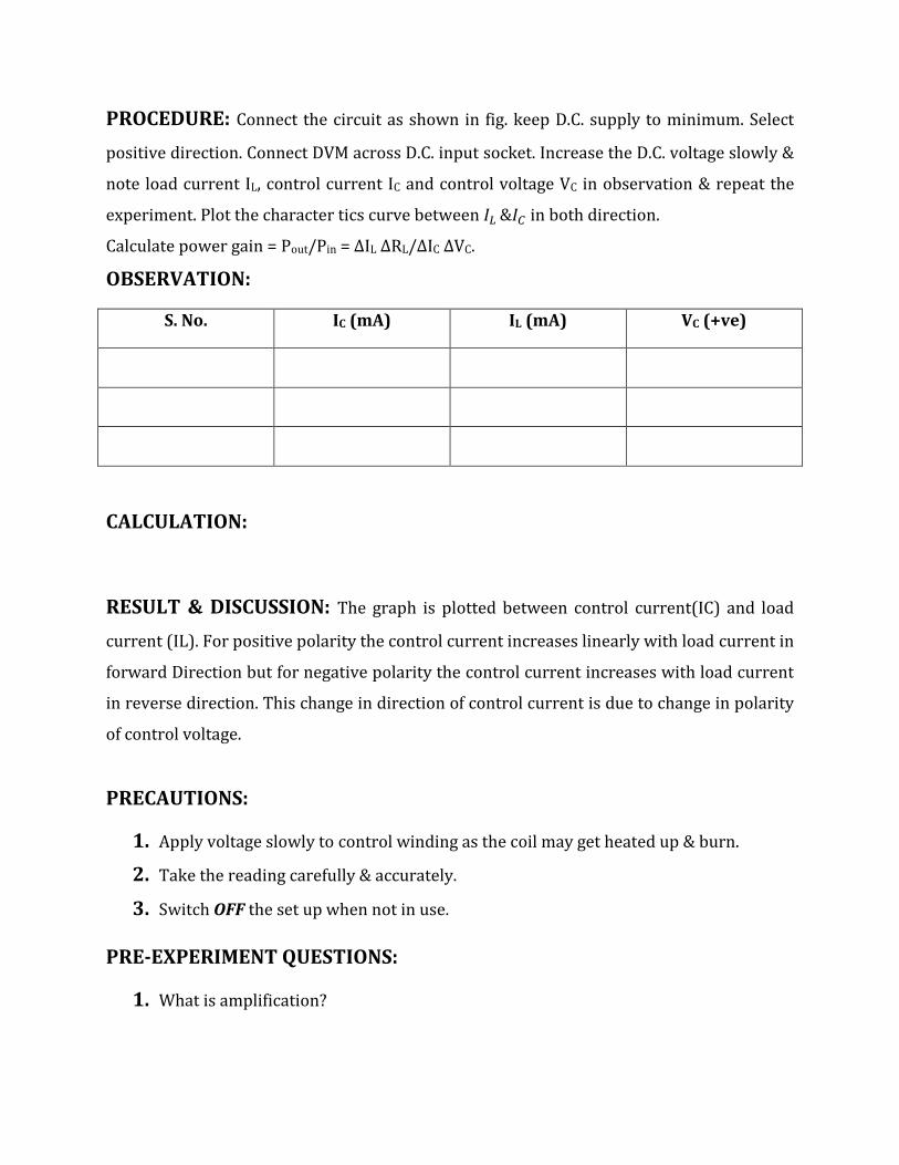
THEORY: Amplification is the control of larger output by variation of a smaller input.

Such amplification can be performed by a magnetic device called magnetic amplifier. This

set up is designed to study basic characteristics of such amplifier. To set up consists of

magnetic amplifier A.C & D.C power supply, to meters for load & control current & fixed

value resistance of 50 ohms.

PROCEDURE: Connect the circuit as shown in fig. keep D.C. supply to minimum. Select

positive direction. Connect DVM across D.C. input socket. Increase the D.C. voltage slowly &

note load current IL, control current IC and control voltage VC in observation & repeat the

experiment. Plot the character tics curve between in both direction.

Calculate power gain = Pout/Pin = ∆IL ∆RL/∆IC ∆VC.

OBSERVATION:

S. No. IC (mA) IL (mA) VC (+ve)

CALCULATION:

RESULT & DISCUSSION: The graph is plotted between control current(IC) and load

current (IL). For positive polarity the control current increases linearly with load current in

forward Direction but for negative polarity the control current increases with load current

in reverse direction. This change in direction of control current is due to change in polarity

of control voltage.

PRECAUTIONS:

1. Apply voltage slowly to control winding as the coil may get heated up & burn.

2. Take the reading carefully & accurately.

3. Switch OFF the set up when not in use.

PRE-EXPERIMENT QUESTIONS:

1. What is amplification?

Ans: Amplification is the control of a larger output quantity by the variation of a smaller input quantity.

2. What is magnetic amplifier?

Ans: Magnetic amplifier is a device which amplifies a small input quantity to a large

output quantity.

3. What is the working principle of magnetic amplifier?

Ans: A magnetic amplifier works on the principle of linkage of induced Magneto Motive

Force (MMF).

4. What is saturable reactor?

Ans: The saturable reactor is a specially wound transformer with three winding

instead of two windings like a common transformer.

POST-EXPERIMENT QUESTIONS:

1. What is drawback of a magnetic amplifier?

Ans: The main drawback of magnetic amplifier is to control small DC current a Large

number of turns is required which has a greater resistance requires large DC voltage.

2. How this problem is overcome in a magnetic amplifier?

Ans: This problem is overcome in a magnetic amplifier by self saturation mode.

3. What is the nature of saturable reactor? Ans: The saturable reactor is inductive in nature.

4. What is effect of sudden current application to control winding? Ans: If a sudden current is applied to the control winding the current and ampere

turns of control winding decreases slowly since it has large inductance

EXPERIMENT NO. 2B

OBJECTIVE: To study Input / Output characteristic of a magnetic amplifier in Self

Saturable Reactormode.

APPARATUS REQUIRED:

S. No. Name of the Equipment Used Specification Quantity

1. Magnetic Amplifier Kit

2. Digital Multimeter

3. Connecting Leads

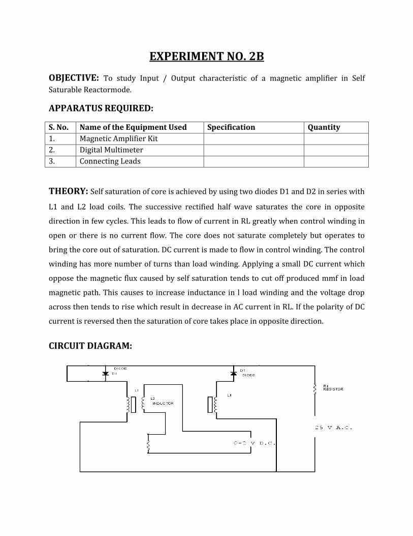
THEORY: Self saturation of core is achieved by using two diodes D1 and D2 in series with

L1 and L2 load coils. The successive rectified half wave saturates the core in opposite

direction in few cycles. This leads to flow of current in RL greatly when control winding in

open or there is no current flow. The core does not saturate completely but operates to

bring the core out of saturation. DC current is made to flow in control winding. The control

winding has more number of turns than load winding. Applying a small DC current which

oppose the magnetic flux caused by self saturation tends to cut off produced mmf in load

magnetic path. This causes to increase inductance in l load winding and the voltage drop

across then tends to rise which result in decrease in AC current in RL. If the polarity of DC

current is reversed then the saturation of core takes place in opposite direction.

CIRCUIT DIAGRAM:

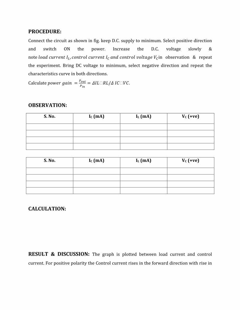
PROCEDURE:

Connect the circuit as shown in fig. keep D.C. supply to minimum. Select positive direction

and switch ON the power. Increase the D.C. voltage slowly &

note in observation & repeat

the experiment. Bring DC voltage to minimum, select negative direction and repeat the

characteristics curve in both directions.

Calculate

OBSERVATION:

S. No. IC (mA) IL (mA) VC (+ve)

S. No. IC (mA) IL (mA) VC (+ve)

CALCULATION:

RESULT & DISCUSSION: The graph is plotted between load current and control

current. For positive polarity the Control current rises in the forward direction with rise in

load current where as for negative polarity the control current decreases in the reverse

direction with rise in load current .This is due to the self saturation of the magnetic core.

PRECAUTIONS:

1. Apply voltage slowly to control winding as the coil may get heated up & burn.

2. Take the reading carefully & accurately.

3. Switch OFF the set up when not in use.

PRE-EXPERIMENT QUESTIONS:

5. What are the modes of operation of the magnetic amplifier?

Ans: The magnetic amplifier operates in two modes, series-parallel mode Self saturation mode.

6. What is the value load resistance RL for magnetic amplifier?

Ans:The value of load resistance RL for magnetic amplifier is 50 ohms Fix.

7. What is core saturation?

Ans: When MMF in a coil is varied due to a varying current it causes the Magnetization

to approach to a limit called saturation.

POST-EXPERIMENT QUESTIONS:

5. What is the direction of windings in the securable reactor?

Ans: In a securable reactor the two windings are anti- phase with each Other.

6. How self saturation is achieved in a magnetic amplifier?

Ans: The self-saturation of core is achieved by using two rectifier diodes D1 & D2 in

series with load coil L1 & L2.

7. How the magnetic core is brought out of saturation? Ans: The core is brought out of saturation by passing a current through Control winding.

8. Which winding has more number of turns? Ans: The control winding has more number of turns than the load Winding.

9. Between which parameter graph is plotted for magnetic amplifier?

Ans:The graph is plotted between load current and control current.

EXPERIMENT NO. 3

AIM: SYNCHRO TRANSMITTER/RECEIVER.

(E) TO STUDY OF SYNCHRO TRANSMITTER IN TERM OF POSITION V/S PHASE AND VOLTAGE MAGNITUDE WITH RESPECT TO ROTAR VOLTAGE MAGNITUDE/PHASE.

(F) TO STUDY OF REMOTE POSITION INDICATION SYSTEM USING SYNCHRO TRANSMITTER/RECEIVER.

APPARATUS REQUIRED:

S. No. Name of the Equipment Used Specification Quantity

1. SYNCHRO TRANSMITTER/RECEIVER KIT

2. A DUAL TRACE CRO

3. MULTIMETER

4. PATCH CORDS

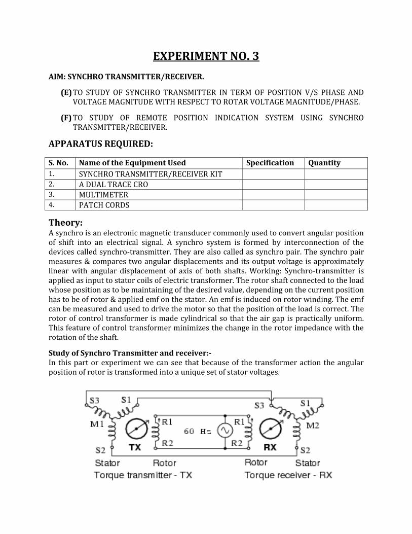
Theory: A synchro is an electronic magnetic transducer commonly used to convert angular position of shift into an electrical signal. A synchro system is formed by interconnection of the devices called synchro-transmitter. They are also called as synchro pair. The synchro pair measures & compares two angular displacements and its output voltage is approximately linear with angular displacement of axis of both shafts. Working: Synchro-transmitter is applied as input to stator coils of electric transformer. The rotor shaft connected to the load whose position as to be maintaining of the desired value, depending on the current position has to be of rotor & applied emf on the stator. An emf is induced on rotor winding. The emf can be measured and used to drive the motor so that the position of the load is correct. The rotor of control transformer is made cylindrical so that the air gap is practically uniform. This feature of control transformer minimizes the change in the rotor impedance with the rotation of the shaft.

Study of Synchro Transmitter and receiver:- In this part or experiment we can see that because of the transformer action the angular position of rotor is transformed into a unique set of stator voltages.

PROCEDURE: FOR EXPERIMENT A

1. Connect the CRO one channel with the provided socket COM and REF. The ground of CRO should be connected to COM. The reference socket is attenuated 1:10, voltage of Tx. with respect to R.

2. Connect CRO other channel with output of S1, S2 and S3 alternatively, while keep Tx. dial to certain position say 0°.

3. Measure the magnitude voltage and phase of stator terminals S1, S2 and S3 with respect to reference with the help of CRO and multimeter. Note them down in the observation table 1.

4. Plot the graphical curve between the voltage/phase of stator terminal.

Table 1:-

Angular Position in Degree

Magnitude/Phase(S1) Magnitude/Phase(S2) Magnitude/Phase(S3)

0°

30°

60°

90°

120°

150°

180°

210°

240°

270°

330°

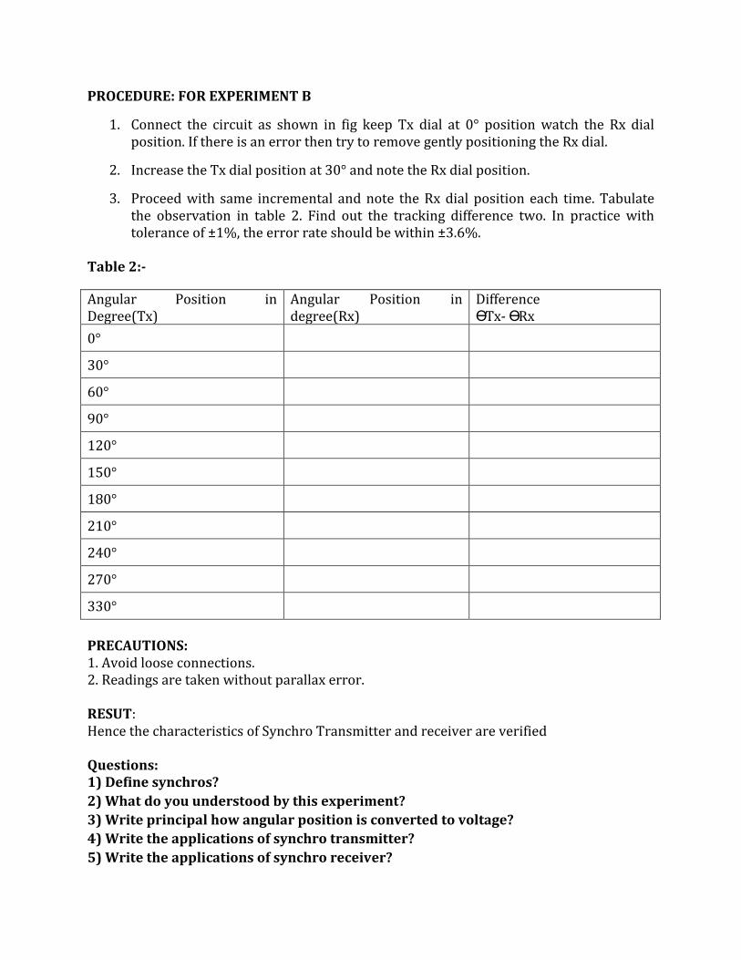
PROCEDURE: FOR EXPERIMENT B

1. Connect the circuit as shown in fig keep Tx dial at 0° position watch the Rx dial position. If there is an error then try to remove gently positioning the Rx dial.

2. Increase the Tx dial position at 30° and note the Rx dial position.

3. Proceed with same incremental and note the Rx dial position each time. Tabulate the observation in table 2. Find out the tracking difference two. In practice with tolerance of ±1%, the error rate should be within ±3.6%.

Table 2:-

Angular Position in Degree(Tx)

Angular Position in degree(Rx)

Difference ϴTx- ϴRx

0°

30°

60°

90°

120°

150°

180°

210°

240°

270°

330°

PRECAUTIONS: 1. Avoid loose connections. 2. Readings are taken without parallax error. RESUT: Hence the characteristics of Synchro Transmitter and receiver are verified Questions: 1) Define synchros?

2) What do you understood by this experiment?

3) Write principal how angular position is converted to voltage?

4) Write the applications of synchro transmitter?

5) Write the applications of synchro receiver?

EXPERIMENT NO. 4

OBJECTIVE: LEAD LAG COMPENSATOR

A. TO STUDY THE OPEN LOOP RESPONSE ON COMPENSATOR.

B. CLOSE LOOP TRANSIENT RESPONSE.

APPARATUS REQUIRED:

S. No. Name of the Equipment

Used

Specification Quantity

1. Lead Lag Compensator Kit

2. Patch Cords

3. CRO

THEORY:

A lead–lag compensator is a component in a control system that improves an undesirable

frequency response in a feedback and control system. It is a fundamental building block in classical

control theory.

Lead–lag compensators influence disciplines as varied as robotics, satellite control, automobile diagnostics, and laser frequency stabilization. They are an important building block in analog control systems, and can also be used in digital control.

Given the control plant, desired specifications can be achieved using compensators. I, D, PI, PD, and PID, are optimizing controllers which are used to improve system parameters (such as reducing steady state error, reducing resonant peak, improving system response by reducing rise time). All these operations can be done by compensators as well.

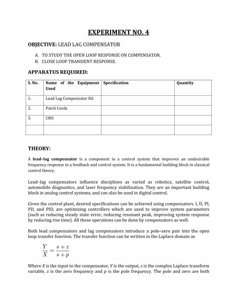
Both lead compensators and lag compensators introduce a pole–zero pair into the open loop transfer function. The transfer function can be written in the Laplace domain as

Where X is the input to the compensator, Y is the output, s is the complex Laplace transform variable, z is the zero frequency and p is the pole frequency. The pole and zero are both

typically negative. In a lead compensator, the pole is left of the zero in the complex plane,

, while in a lag compensator .

A lead-lag compensator consists of a lead compensator cascaded with a lag compensator. The overall transfer function can be written as

Typically , where z1 and p1 are the zero and pole of the lead compensator and z2 and p2 are the zero and pole of the lag compensator. The lead compensator provides phase lead at high frequencies. This shifts the poles to the left, which enhances the responsiveness and stability of the system. The lag compensator provides phase lag at low frequencies which reduces the steady state error.

The precise locations of the poles and zeros depend on both the desired characteristics of the closed loop response and the characteristics of the system being controlled. However, the pole and zero of the lag compensator should be close together so as not to cause the poles to shift right, which could cause instability or slow convergence. Since their purpose is to affect the low frequency behaviour, they should be near the origin.

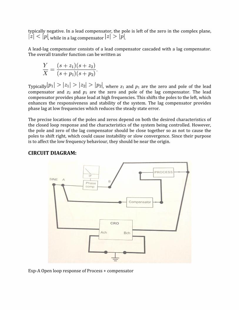
CIRCUIT DIAGRAM:

Exp-A Open loop response of Process + compensator

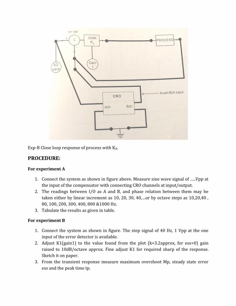
Exp-B Close loop response of process with KA.

PROCEDURE:

For experiment A

1. Connect the system as shown in figure above. Measure sine wave signal of …..Vpp at

the input of the compensator with connecting CRO channels at input/output.

2. The readings between I/O as A and B, and phase relation between them may be

taken either by linear increment as 10, 20, 30, 40,…or by octave steps as 10,20,40 ,

80, 100, 200, 300, 400, 800 &1000 Hz.

3. Tabulate the results as given in table.

For experiment B

1. Connect the system as shown in figure. The step signal of 40 Hz, 1 Vpp at the one

input of the error detector is available.

2. Adjust K1(gain1) to the value found from the plot (k=3.2approx, for ess=0) gain

raised to 10dB/octave approx. Fine adjust K1 for required sharp of the response.

Sketch it on paper.

3. From the transient response measure maximum overshoot Mp, steady state error

ess and the peak time tp.

OBSERVATION:

Table for plotting of response curve plant +(Lag)

Freq A Vpp B Vpp Gain dB Φº

10

20

40

80

Table for plotting of response curve plant +(Lead)

Freq A Vpp B Vpp Gain dB Φº

10

20

40

80

CALCULATION:

RESULT & DISCUSSION:

Hence the characteristics of Lead- Lag compensator are verified.

PRECAUTIONS:

1. Avoid loose connections. 2. Readings are taken without parallax error.

PRE-EXPERIMENT QUESTIONS:

1. Write a brief note about Lag Compensator.

2. Write a brief note about Lead Compensator.

3. Write a brief note about Lag Lead Compensator.

4 The max. phase shift provided for lead compensator with transfer function

G(s)=(1+6s)/(1+2s)

5. Which compensation is adopted for improving transient response of a negative unity feedback

system?

6. Which compensation is adopted for improving steady response of a negative unity feedback

system?

7. Which compensation is adopted for improving both steady state and transient response of a

negative unity feedback system?

8. What happens to the gain crossover frequency when phase lag compensator is used?

9. What happens to the gain crossover frequency when phase lead compensator is used?

10. What is the effect of phase lag compensation on servo system performance?

POST-EXPERIMENT QUESTIONS:

EXPERIMENT NO. 5

OBJECTIVE: LINEAR SYSTEM SIMULATOR

(G) OPEN LOOP RESPONSE I. ERROR DETECTOR WITH GAIN

II. TIME CONSTANT III. INTEGRATOR

(H) CLOSED LOOP SYSTEM I. FIRST ORDER SYSTEM

II. SECOND ORDER SYSTEM III. THIRD ORDER SYSTEM

APPARATUS REQUIRED:

S. No. Name of the Equipment Used Specification Quantity

1. Linear System simulator Kit

2. CRO

3. Patch Cords

THEORY:

Oscillating systems whose properties do not change when their state changes—that is, the parameters of a linear system that characterize its properties (the elasticity, mass, and coefficient of friction of a mechanical system; the capacitance, inductance, and active resistance of an electrical system) are independent of the quantities that characterize its state.

The parameters of real systems always depend to some extent on state. For example, the coefficient of elasticity of a spring depends on the magnitude of the, and the active resistance of a conductor depends on its temperature, which in turn depends on the strength of the current passing through the conductor. Therefore, real systems may be considered linear only within certain limits of changes in their state for which changes in their parameters may be disregarded. For a very large number of real systems these limits prove to be extremely broad, and therefore most problems can be solved by regarding real systems as linear. Examples of linear systems are a pendulum, an electrical oscillatory circuit, a bridge measuring circuit, and automatic control systems. When changes in the parameters of a real system appear within the limits of possible changes in its state, the nonlinearity of the system must be taken into account.

Linear systems have properties that greatly simplify analysis of processes that transpire within them. Processes in linear systems are described by linear differential equations. In physically different linear systems processes are described by structurally identical equations. This is the basis for physical and, in particular, electrical simulation of linear systems and computer simulation. Linear systems play a major role in physics and engineering, since they reproduce without distortion of form external influences that have the character of harmonic oscillations and because the superposition principle is valid in them.

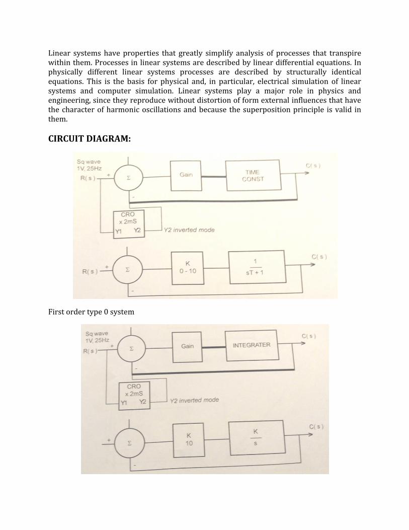
CIRCUIT DIAGRAM:

First order type 0 system

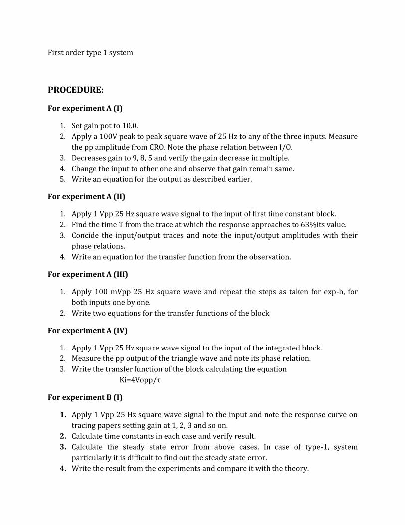
First order type 1 system

PROCEDURE:

For experiment A (I)

1. Set gain pot to 10.0.

2. Apply a 100V peak to peak square wave of 25 Hz to any of the three inputs. Measure

the pp amplitude from CRO. Note the phase relation between I/O.

3. Decreases gain to 9, 8, 5 and verify the gain decrease in multiple.

4. Change the input to other one and observe that gain remain same.

5. Write an equation for the output as described earlier.

For experiment A (II)

1. Apply 1 Vpp 25 Hz square wave signal to the input of first time constant block.

2. Find the time T from the trace at which the response approaches to 63%its value.

3. Concide the input/output traces and note the input/output amplitudes with their

phase relations.

4. Write an equation for the transfer function from the observation.

For experiment A (III)

1. Apply 100 mVpp 25 Hz square wave and repeat the steps as taken for exp-b, for

both inputs one by one.

2. Write two equations for the transfer functions of the block.

For experiment A (IV)

1. Apply 1 Vpp 25 Hz square wave signal to the input of the integrated block.

2. Measure the pp output of the triangle wave and note its phase relation.

3. Write the transfer function of the block calculating the equation

Ki=4Vopp/τ

For experiment B (I)

1. Apply 1 Vpp 25 Hz square wave signal to the input and note the response curve on

tracing papers setting gain at 1, 2, 3 and so on.

2. Calculate time constants in each case and verify result.

3. Calculate the steady state error from above cases. In case of type-1, system

particularly it is difficult to find out the steady state error.

4. Write the result from the experiments and compare it with the theory.

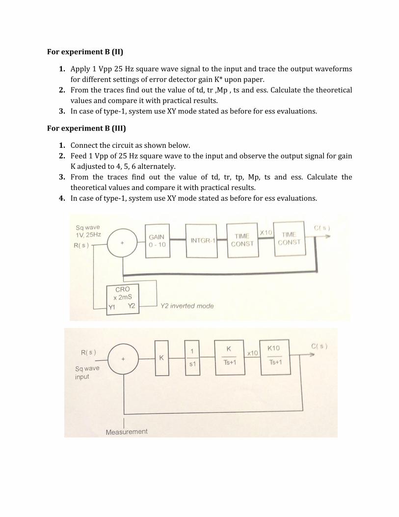
For experiment B (II)

1. Apply 1 Vpp 25 Hz square wave signal to the input and trace the output waveforms

for different settings of error detector gain K* upon paper.

2. From the traces find out the value of td, tr ,Mp , ts and ess. Calculate the theoretical

values and compare it with practical results.

3. In case of type-1, system use XY mode stated as before for ess evaluations.

For experiment B (III)

1. Connect the circuit as shown below.

2. Feed 1 Vpp of 25 Hz square wave to the input and observe the output signal for gain

K adjusted to 4, 5, 6 alternately.

3. From the traces find out the value of td, tr, tp, Mp, ts and ess. Calculate the

theoretical values and compare it with practical results.

4. In case of type-1, system use XY mode stated as before for ess evaluations.

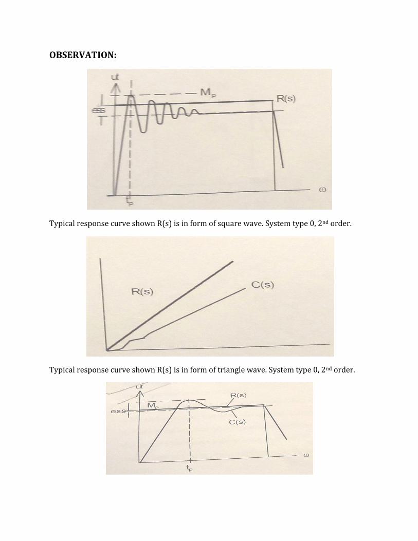
OBSERVATION:

Typical response curve shown R(s) is in form of square wave. System type 0, 2nd order.

Typical response curve shown R(s) is in form of triangle wave. System type 0, 2nd order.

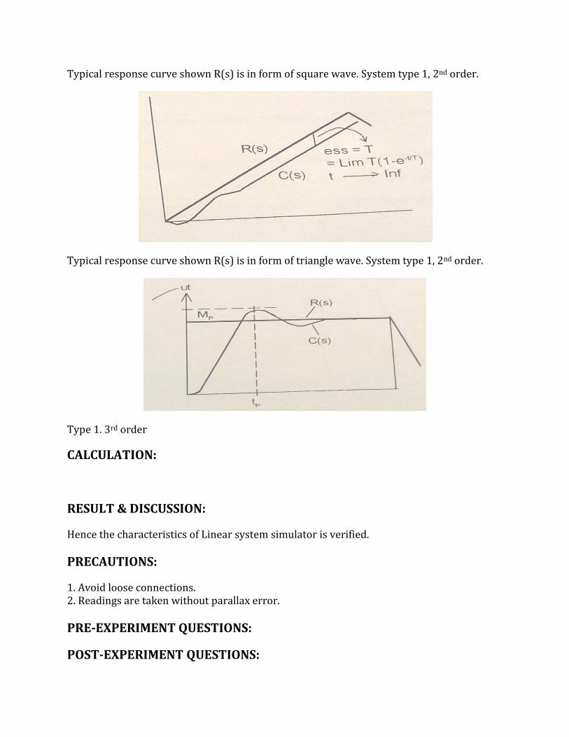
Typical response curve shown R(s) is in form of square wave. System type 1, 2nd order.

Typical response curve shown R(s) is in form of triangle wave. System type 1, 2nd order.

Type 1. 3rd order

CALCULATION:

RESULT & DISCUSSION:

Hence the characteristics of Linear system simulator is verified.

PRECAUTIONS:

1. Avoid loose connections. 2. Readings are taken without parallax error.

PRE-EXPERIMENT QUESTIONS:

POST-EXPERIMENT QUESTIONS:

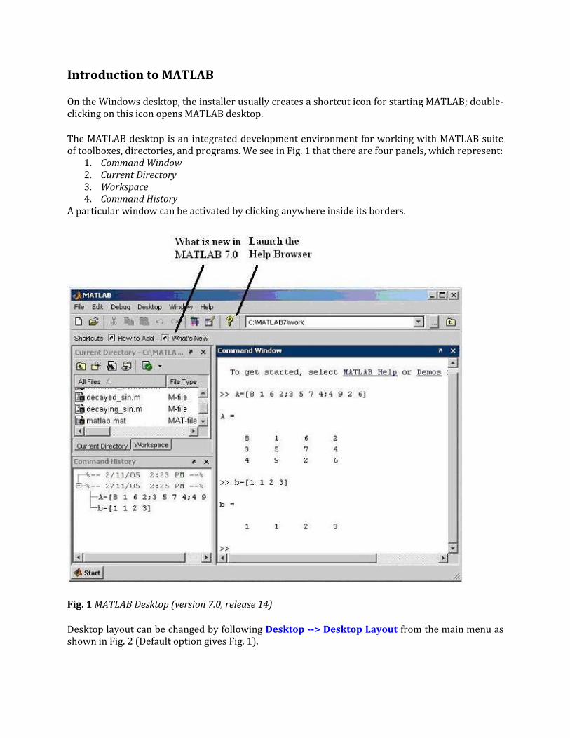
Introduction to MATLAB

On the Windows desktop, the installer usually creates a shortcut icon for starting MATLAB; double-clicking on this icon opens MATLAB desktop.

The MATLAB desktop is an integrated development environment for working with MATLAB suite of toolboxes, directories, and programs. We see in Fig. 1 that there are four panels, which represent:

1. Command Window 2. Current Directory 3. Workspace 4. Command History

A particular window can be activated by clicking anywhere inside its borders.

Fig. 1 MATLAB Desktop (version 7.0, release 14)

Desktop layout can be changed by following Desktop --> Desktop Layout from the main menu as shown in Fig. 2 (Default option gives Fig. 1).

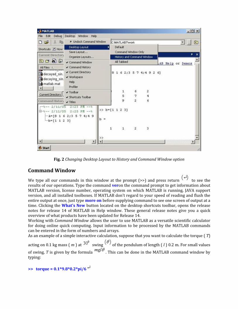
Fig. 2 Changing Desktop Layout to History and Command Window option

Command Window

We type all our commands in this window at the prompt (>>) and press return to see the results of our operations. Type the command veron the command prompt to get information about MATLAB version, license number, operating system on which MATLAB is running, JAVA support version, and all installed toolboxes. If MATLAB don't regard to your speed of reading and flush the entire output at once, just type more on before supplying command to see one screen of output at a time. Clicking the What's New button located on the desktop shortcuts toolbar, opens the release notes for release 14 of MATLAB in Help window. These general release notes give you a quick overview of what products have been updated for Release 14. Working with Command Window allows the user to use MATLAB as a versatile scientific calculator for doing online quick computing. Input information to be processed by the MATLAB commands can be entered in the form of numbers and arrays. As an example of a simple interactive calculation, suppose that you want to calculate the torque ( T)

acting on 0.1 kg mass ( m ) at swing of the pendulum of length ( l ) 0.2 m. For small values

of swing, T is given by the formula . This can be done in the MATLAB command window by typing:

>> torque = 0.1*9.8*0.2*pi/6

MATLAB responds to this command by:

torque =

0.1026

MATLAB calculates and stores the answer in a variable torque (in fact, a array) as soon as the

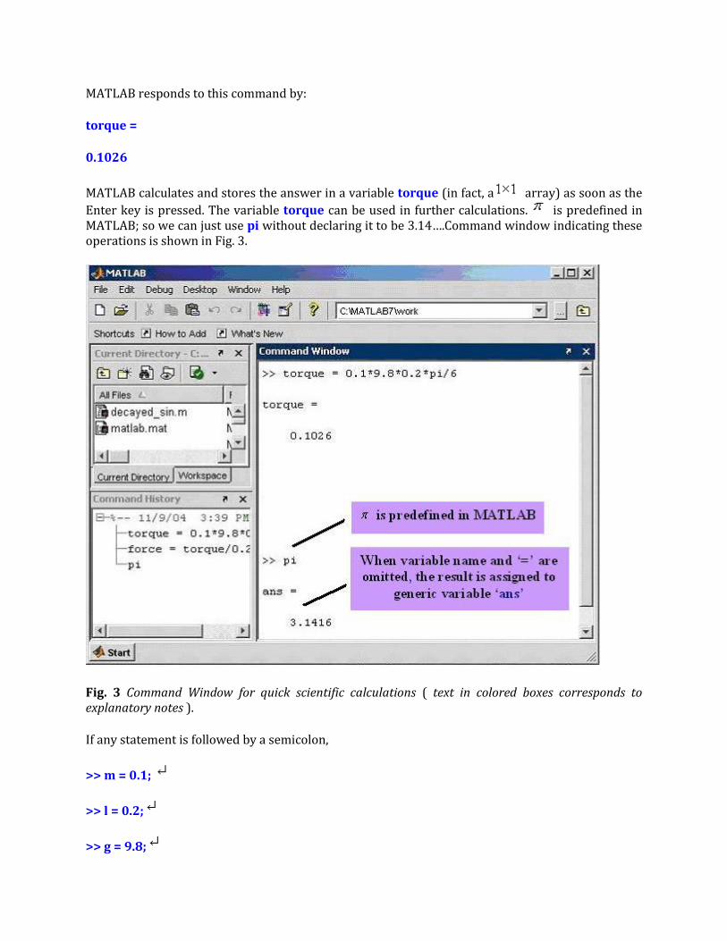
Enter key is pressed. The variable torque can be used in further calculations. is predefined in MATLAB; so we can just use pi without declaring it to be 3.14….Command window indicating these operations is shown in Fig. 3.

Fig. 3 Command Window for quick scientific calculations ( text in colored boxes corresponds to explanatory notes ).

If any statement is followed by a semicolon,

>> m = 0.1;

>> l = 0.2;

>> g = 9.8;

the display of the result is suppressed. The assignment of the variable has been carried out even though the display is suppressed by the semicolon. To view the assignment of a variable, simply type the variable name and hit Enter. For example:

>>torque=m*g*l*pi/6;

>>torque

torque =

0.1026

It is often the case that your MATLAB sessions will include intermediate calculations whose display is of little interest. Output display management has the added benefit of increasing the execution speed of the calculations, since displaying screen output takes time.

Variable names begin with a letter and are followed by any number of letters or numbers (including underscore). Keep the name length to 31 characters, since MATLAB remembers only the first 31 characters. Generally we do not use extremely long variable names even though they may be legal MATLAB names. Since MATLAB is case sensitive, the variables Aand aare different.

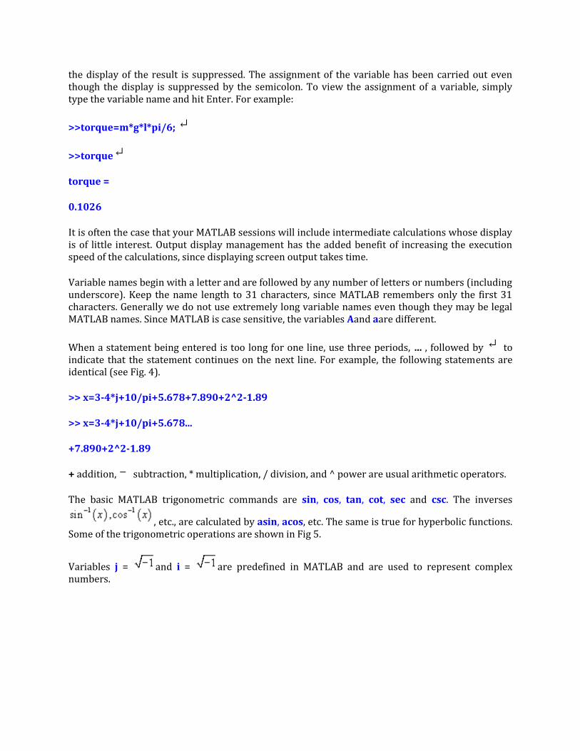
When a statement being entered is too long for one line, use three periods, … , followed by to indicate that the statement continues on the next line. For example, the following statements are identical (see Fig. 4).

>> x=3-4*j+10/pi+5.678+7.890+2^2-1.89

>> x=3-4*j+10/pi+5.678...

+7.890+2^2-1.89

+ addition, subtraction, * multiplication, / division, and ^ power are usual arithmetic operators.

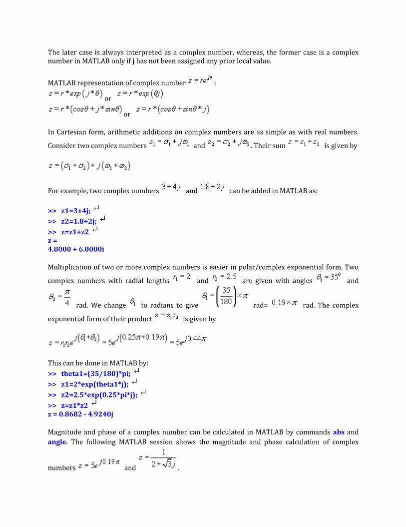
The basic MATLAB trigonometric commands are sin, cos, tan, cot, sec and csc. The inverses

, etc., are calculated by asin, acos, etc. The same is true for hyperbolic functions. Some of the trigonometric operations are shown in Fig 5.

Variables j = and i = are predefined in MATLAB and are used to represent complex numbers.

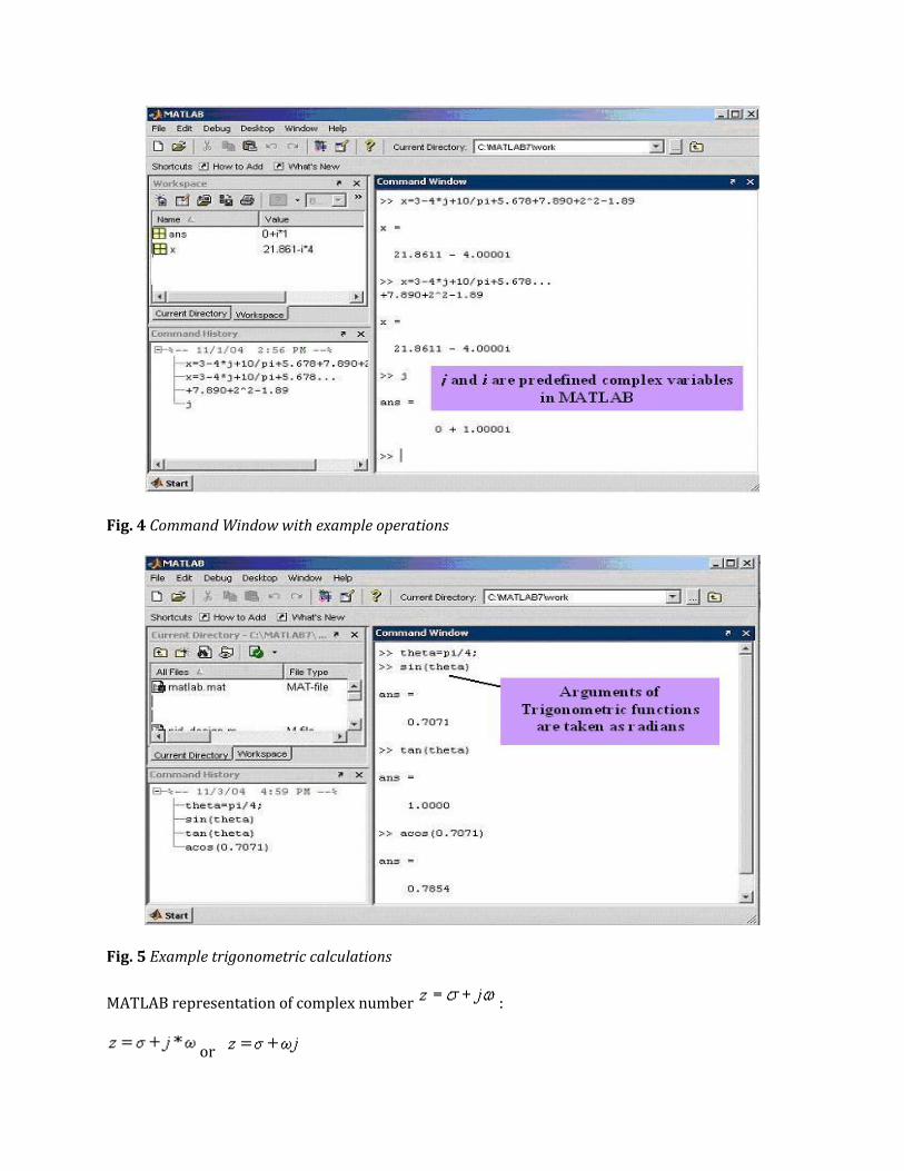
Fig. 4 Command Window with example operations

Fig. 5 Example trigonometric calculations

MATLAB representation of complex number :

or

The later case is always interpreted as a complex number, whereas, the former case is a complex number in MATLAB only if j has not been assigned any prior local value.

MATLAB representation of complex number :

or

or

In Cartesian form, arithmetic additions on complex numbers are as simple as with real numbers.

Consider two complex numbers and . Their sum is given by

For example, two complex numbers and can be added in MATLAB as:

>> z1=3+4j;

>> z2=1.8+2j;

>> z=z1+z2 z = 4.8000 + 6.0000i

Multiplication of two or more complex numbers is easier in polar/complex exponential form. Two

complex numbers with radial lengths and are given with angles and

rad. We change to radians to give rad= rad. The complex

exponential form of their product is given by

This can be done in MATLAB by:

>> theta1=(35/180)*pi;

>> z1=2*exp(theta1*j);

>> z2=2.5*exp(0.25*pi*j);

>> z=z1*z2 z = 0.8682 - 4.9240j

Magnitude and phase of a complex number can be calculated in MATLAB by commands abs and

angle. The following MATLAB session shows the magnitude and phase calculation of complex

numbers and .

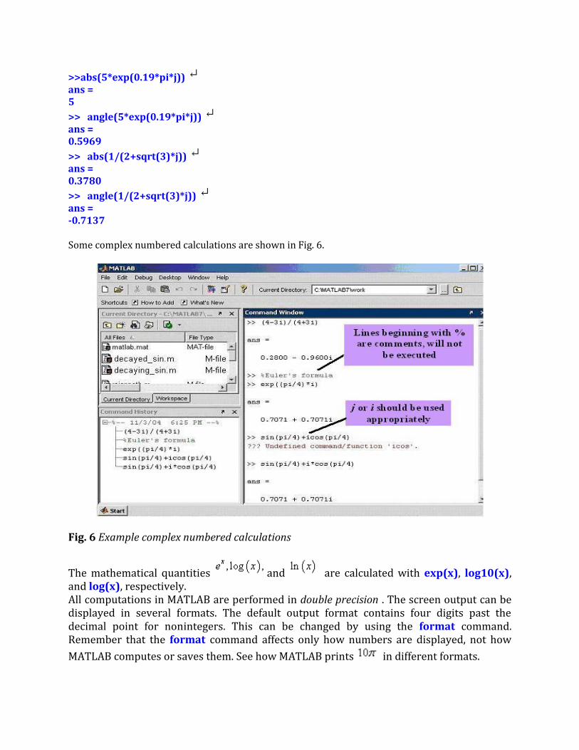
>>abs(5*exp(0.19*pi*j)) ans = 5

>> angle(5*exp(0.19*pi*j)) ans = 0.5969

>> abs(1/(2+sqrt(3)*j)) ans = 0.3780

>> angle(1/(2+sqrt(3)*j)) ans = -0.7137 Some complex numbered calculations are shown in Fig. 6.

Fig. 6 Example complex numbered calculations

The mathematical quantities and are calculated with exp(x), log10(x), and log(x), respectively. All computations in MATLAB are performed in double precision . The screen output can be displayed in several formats. The default output format contains four digits past the decimal point for nonintegers. This can be changed by using the format command. Remember that the format command affects only how numbers are displayed, not how

MATLAB computes or saves them. See how MATLAB prints in different formats.

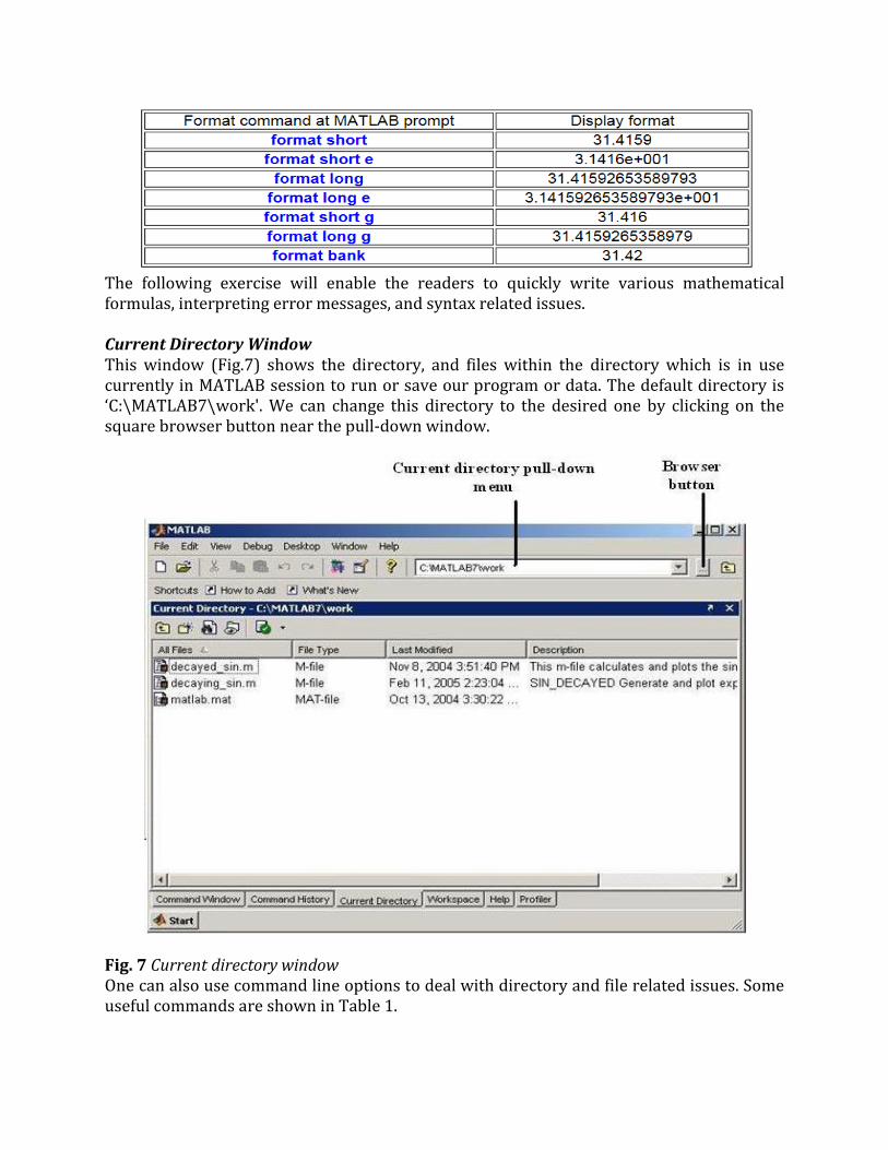
The following exercise will enable the readers to quickly write various mathematical formulas, interpreting error messages, and syntax related issues. Current Directory Window This window (Fig.7) shows the directory, and files within the directory which is in use currently in MATLAB session to run or save our program or data. The default directory is ‘C:\MATLAB7\work'. We can change this directory to the desired one by clicking on the square browser button near the pull-down window.

Fig. 7 Current directory window One can also use command line options to deal with directory and file related issues. Some useful commands are shown in Table 1.

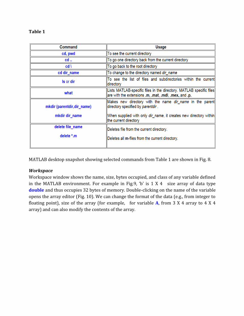
Table 1

MATLAB desktop snapshot showing selected commands from Table 1 are shown in Fig. 8.

Workspace

Workspace window shows the name, size, bytes occupied, and class of any variable defined

in the MATLAB environment. For example in Fig.9, ‘b' is 1 X 4 size array of data type

double and thus occupies 32 bytes of memory. Double-clicking on the name of the variable

opens the array editor (Fig. 10). We can change the format of the data (e.g., from integer to

floating point), size of the array (for example, for variable A, from 3 X 4 array to 4 X 4

array) and can also modify the contents of the array.

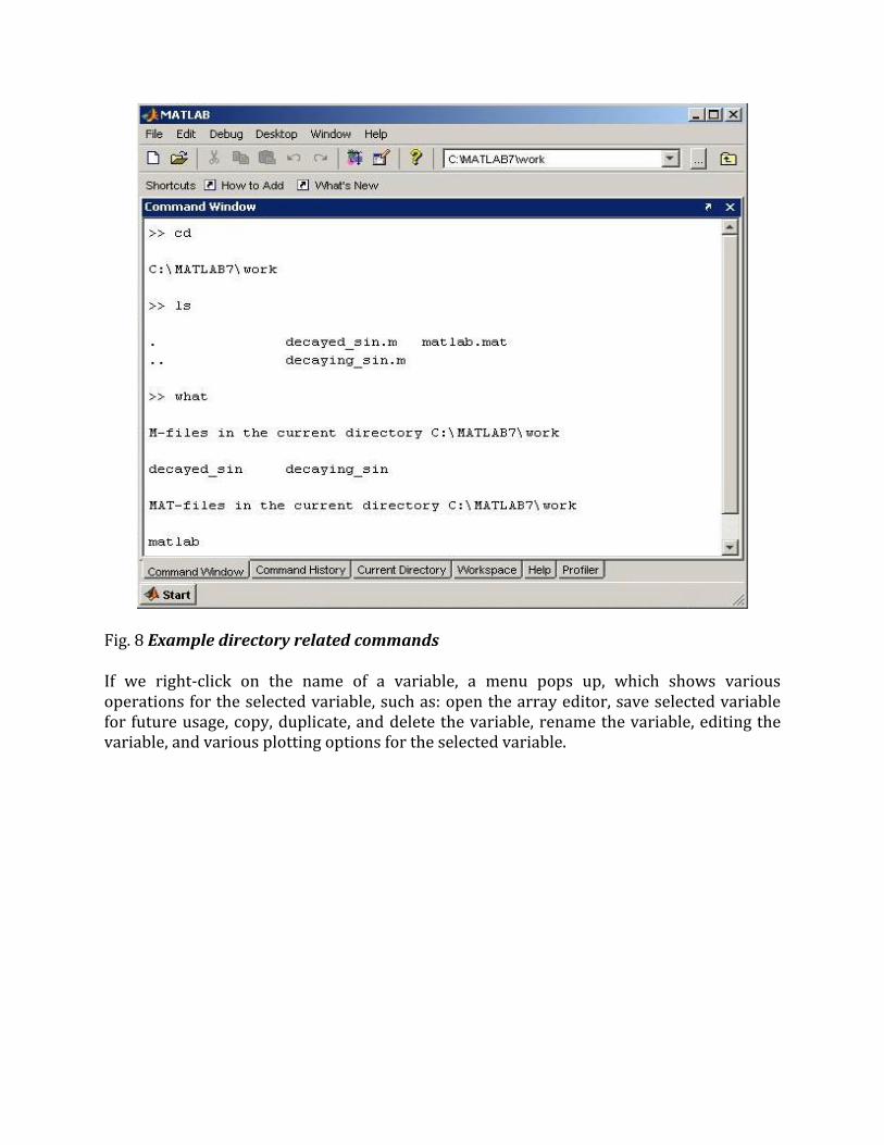
Fig. 8 Example directory related commands

If we right-click on the name of a variable, a menu pops up, which shows various operations for the selected variable, such as: open the array editor, save selected variable for future usage, copy, duplicate, and delete the variable, rename the variable, editing the variable, and various plotting options for the selected variable.

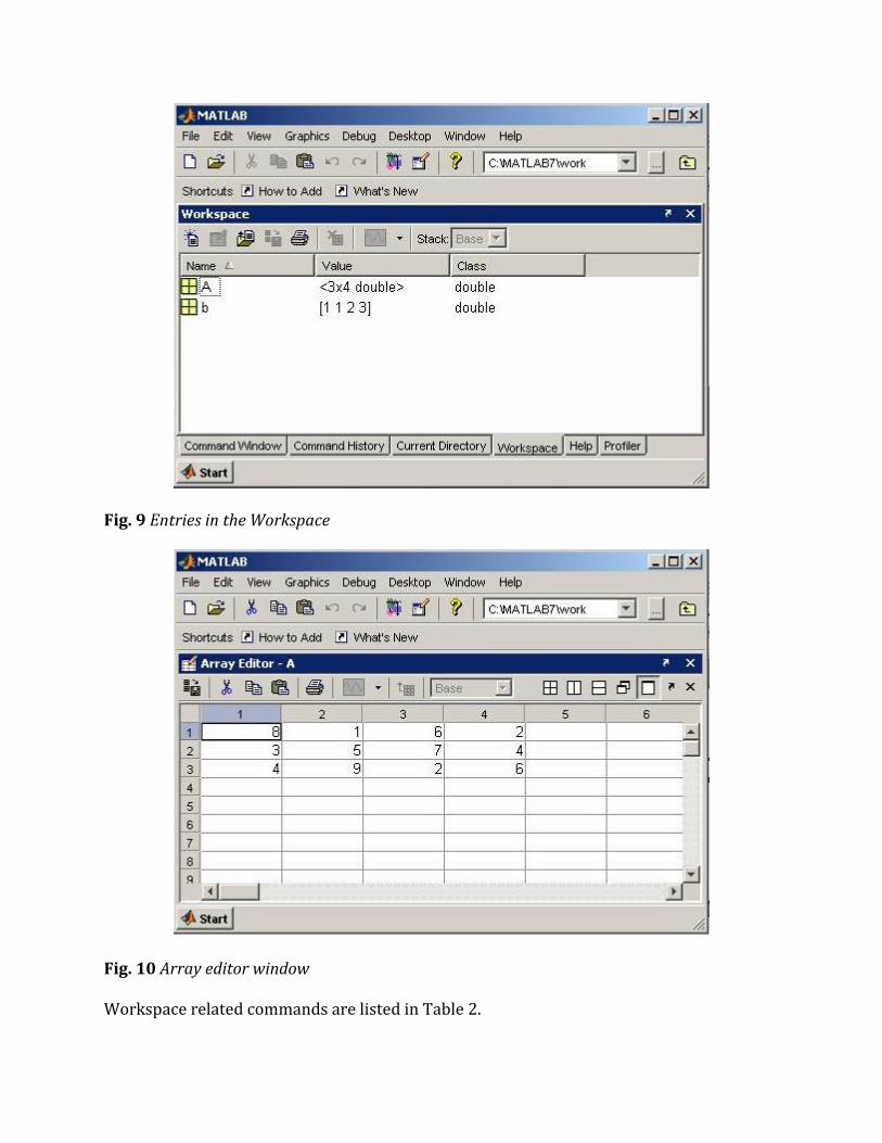
Fig. 9 Entries in the Workspace

Fig. 10 Array editor window

Workspace related commands are listed in Table 2.

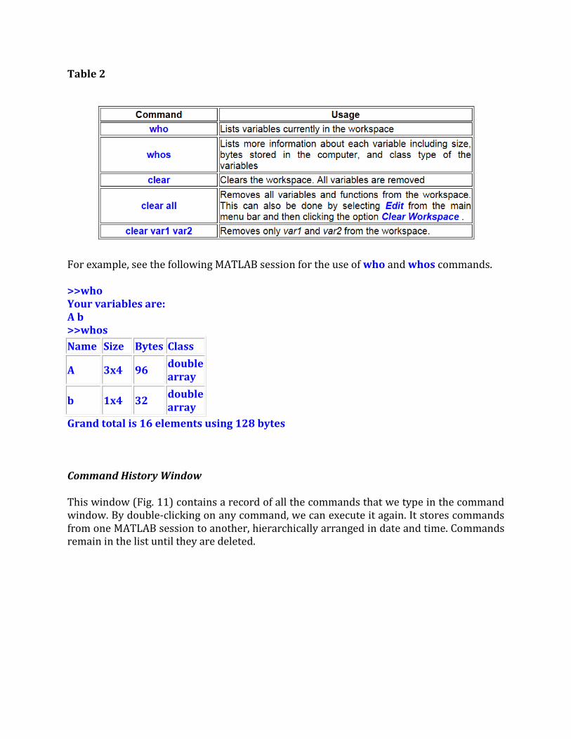
Table 2

For example, see the following MATLAB session for the use of who and whos commands.

>>who Your variables are: A b >>whos

Name Size Bytes Class

A 3x4 96 double array

b 1x4 32 double array

Grand total is 16 elements using 128 bytes

Command History Window

This window (Fig. 11) contains a record of all the commands that we type in the command window. By double-clicking on any command, we can execute it again. It stores commands from one MATLAB session to another, hierarchically arranged in date and time. Commands remain in the list until they are deleted.

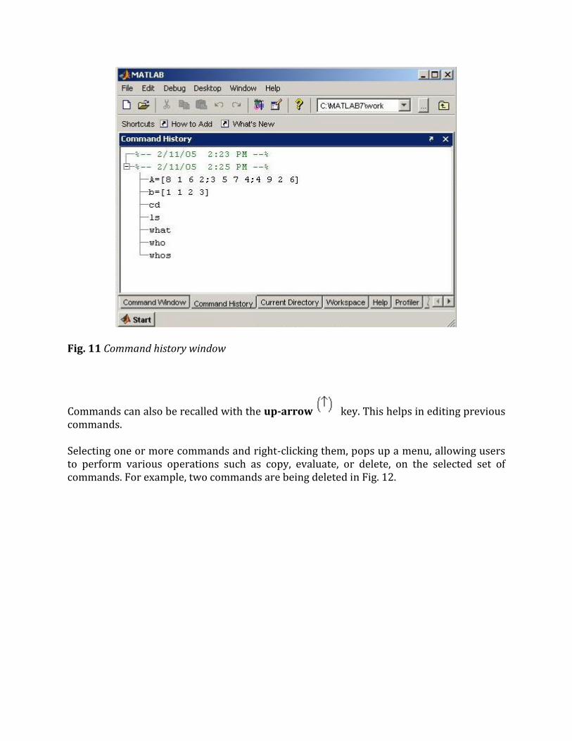
Fig. 11 Command history window

Commands can also be recalled with the up-arrow key. This helps in editing previous commands.

Selecting one or more commands and right-clicking them, pops up a menu, allowing users to perform various operations such as copy, evaluate, or delete, on the selected set of commands. For example, two commands are being deleted in Fig. 12.

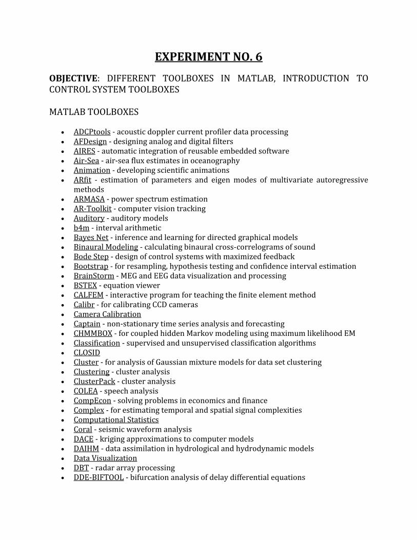
EXPERIMENT NO. 6

OBJECTIVE: DIFFERENT TOOLBOXES IN MATLAB, INTRODUCTION TO CONTROL SYSTEM TOOLBOXES MATLAB TOOLBOXES

ADCPtools - acoustic doppler current profiler data processing AFDesign - designing analog and digital filters AIRES - automatic integration of reusable embedded software Air-Sea - air-sea flux estimates in oceanography Animation - developing scientific animations ARfit - estimation of parameters and eigen modes of multivariate autoregressive

methods ARMASA - power spectrum estimation AR-Toolkit - computer vision tracking Auditory - auditory models b4m - interval arithmetic Bayes Net - inference and learning for directed graphical models Binaural Modeling - calculating binaural cross-correlograms of sound Bode Step - design of control systems with maximized feedback Bootstrap - for resampling, hypothesis testing and confidence interval estimation BrainStorm - MEG and EEG data visualization and processing BSTEX - equation viewer CALFEM - interactive program for teaching the finite element method Calibr - for calibrating CCD cameras Camera Calibration Captain - non-stationary time series analysis and forecasting CHMMBOX - for coupled hidden Markov modeling using maximum likelihood EM Classification - supervised and unsupervised classification algorithms CLOSID Cluster - for analysis of Gaussian mixture models for data set clustering Clustering - cluster analysis ClusterPack - cluster analysis COLEA - speech analysis CompEcon - solving problems in economics and finance Complex - for estimating temporal and spatial signal complexities Computational Statistics Coral - seismic waveform analysis DACE - kriging approximations to computer models DAIHM - data assimilation in hydrological and hydrodynamic models Data Visualization DBT - radar array processing DDE-BIFTOOL - bifurcation analysis of delay differential equations

Denoise - for removing noise from signals DiffMan - solving differential equations on manifolds Dimensional Analysis - DIPimage - scientific image processing Direct - Laplace transform inversion via the direct integration method DirectSD - analysis and design of computer controlled systems with process-

oriented models DMsuite - differentiation matrix suite DMTTEQ - design and test time domain equalizer design methods DrawFilt - drawing digital and analog filters DSFWAV - spline interpolation with Dean wave solutions DWT - discrete wavelet transforms EasyKrig Econometrics EEGLAB EigTool - graphical tool for non symmetriceigen problems EMSC - separating light scattering and absorbance by extended multiplicative signal

correction Engineering Vibration FastICA - fixed-point algorithm for ICA and projection pursuit FDC - flight dynamics and control FDtools - fractional delay filter design FlexICA - for independent components analysis FMBPC - fuzzy model-based predictive control ForWaRD - Fourier-wavelet regularized deconvolution FracLab - fractal analysis for signal processing FSBOX - stepwise forward and backward selection of features using linear

regression GABLE - geometric algebra tutorial GAOT - genetic algorithm optimization Garch - estimating and diagnosing heteroskedasticity in time series models GCE Data - managing, analyzing and displaying data and metadata stored using the

GCE data structure specification GCSV - growing cell structure visualization GEMANOVA - fitting multilinear ANOVA models Genetic Algorithm Geodetic - geodetic calculations GHSOM - growing hierarchical self-organizing map glmlab - general linear models GPIB - wrapper for GPIB library from National Instrument GTM - generative topographic mapping, a model for density modeling and data

visualization GVF - gradient vector flow for finding 3-D object boundaries HFRadarmap - converts HF radar data from radial current vectors to total vectors HFRC - importing, processing and manipulating HF radar data Hilbert - Hilbert transform by the rational eigenfunction expansion method

HMM - hidden Markov models HMMBOX - for hidden Markov modeling using maximum likelihood EM HUTear - auditory modeling ICALAB - signal and image processing using ICA and higher order statistics Imputation - analysis of incomplete datasets IPEM - perception based musical analysis JMatLink - Matlab Java classes Kalman - Bayesian Kalman filter Kalman Filter - filtering, smoothing and parameter estimation (using EM) for linear

dynamical systems KALMTOOL - state estimation of nonlinear systems Kautz - Kautz filter design Kriging LDestimate - estimation of scaling exponents LDPC - low density parity check codes LHS - Latin Hypercube Sampling, an efficient Monte Carlo method LISQ - wavelet lifting scheme on quincunx grids LKER - Laguerre kernel estimation tool LMAM-OLMAM - Levenberg Marquardt with Adaptive Momentum algorithm for

training feedforward neural networks Low-Field NMR - for exponential fitting, phase correction of quadrature data and

slicing LPSVM - Newton method for LP support vector machine for machine learning

problems LSDPTOOL - robust control system design using the loop shaping design procedure LS-SVMlab LSVM - Lagrangian support vector machine for machine learning problems Lyngby - functional neuroimaging MARBOX - for multivariate autogressive modeling and cross-spectral estimation MatArray - analysis of microarray data Matrix Computation - constructing test matrices, computing matrix factorizations,

visualizing matrices, and direct search optimization MCAT - Monte Carlo analysis MDP - Markov decision processes MESHPART - graph and mesh partioning methods MILES - maximum likelihood fitting using ordinary least squares algorithms MIMO - multidimensional code synthesis Missing - functions for handling missing data values M_Map - geographic mapping tools MODCONS - multi-objective control system design MOEA - multi-objective evolutionary algorithms MS - estimation of multiscaling exponents Multiblock - analysis and regression on several data blocks simultaneously Multiscale Shape Analysis Music Analysis - feature extraction from raw audio signals for content-based music

retrieval

MWM - multifractal wavelet model NetCDF Netlab - neural network algorithms NiDAQ - data acquisition using the NiDAQ library NEDM - nonlinear economic dynamic models NMM - numerical methods in Matlab text NNCTRL - design and simulation of control systems based on neural networks NNSYSID - neural net based identification of nonlinear dynamic systems NSVM - newton support vector machine for solving machine learning problems NURBS - non-uniform rational B-splines N-way - analysis of multiway data with multilinear models OpenFEM - finite element development PCNN - pulse coupled neural networks Peruna - signal processing and analysis PhiVis - probabilistic hierarchical interactive visualization, i.e. functions for visual

analysis of multivariate continuous data Planar Manipulator - simulation of n-DOF planar manipulators PRTools - pattern recognition psignifit - testing hyptheses about psychometric functions PSVM - proximal support vector machine for solving machine learning problems Psychophysics - vision research PyrTools - multi-scale image processing RBF - radial basis function neural networks RBN - simulation of synchronous and asynchronous random boolean networks ReBEL - sigma-point Kalman filters Regression - basic multivariate data analysis and regression Regularization Tools Regularization Tools XP Restore Tools Robot - robotics functions, e.g. kinematics, dynamics and trajectory generation Robust Calibration - robust calibration in stats RRMT - rainfall-runoff modelling SAM - structure and motion Schwarz-Christoffel - computation of conformal maps to polygonally bounded

regions SDH - smoothed data histogram SeaGrid - orthogonal grid maker SEA-MAT - oceanographic analysis SLS - sparse least squares SolvOpt - solver for local optimization problems SOM - self-organizing map SOSTOOLS - solving sums of squares (SOS) optimization problems Spatial and Geometric Analysis Spatial Regression Spatial Statistics Spectral Methods

SPM - statistical parametric mapping SSVM - smooth support vector machine for solving machine learning problems STATBAG - for linear regression, feature selection, generation of data, and

significance testing StatBox - statistical routines Statistical Pattern Recognition - pattern recognition methods Stixbox - statistics SVM - implements support vector machines SVM Classifier Symbolic Robot Dynamics TEMPLAR - wavelet-based template learning and pattern classification TextClust - model-based document clustering TextureSynth - analyzing and synthesizing visual textures TfMin - continous 3-D minimum time orbit transfer around Earth Time-Frequency - analyzing non-stationary signals using time-frequency

distributions Tree-Ring - tasks in tree-ring analysis TSA - uni- and multivariate, stationary and non-stationary time series analysis TSTOOL - nonlinear time series analysis T_Tide - harmonic analysis of tides UTVtools - computing and modifying rank-revealing URV and UTV decompositions Uvi_Wave - wavelet analysis varimax - orthogonal rotation of EOFs VBHMM - variation Bayesian hidden Markov models VBMFA - variational Bayesian mixtures of factor analyzers VMT - VRML Molecule Toolbox, for animating results from molecular dynamics

experiments VRMLplot - generates interactive VRML 2.0 graphs and animations VSVtools - computing and modifying symmetric rank-revealing decompositions WAFO - wave analysis for fatique and oceanography WarpTB - frequency-warped signal processing WAVEKIT - wavelet analysis WaveLab - wavelet analysis Weeks - Laplace transform inversion via the Weeks method WetCDF - NetCDF interface WHMT - wavelet-domain hidden Markov tree models WInHD - Wavelet-based inverse halftoning via deconvolution WSCT - weighted sequences clustering toolkit XMLTree - XML parser YAADA - analyze single particle mass spectrum data ZMAP - quantitative seismicity analysis

CONTROL SYSTEM TOOL BOXES Design and analyze control systems

Getting Started

Examples

Release Notes

Linear System Representation

Models of linear time-invariant systems

o Basic Models

o Tunable Models

o Models with Time Delays

o Model Attributes

o Model Arrays

Model Interconnection

Series, parallel, and feedback connections; block diagram building

Functions

feedback Feedback connection of two models

connect Block diagram interconnections of dynamic systems

sumblk Summing junction for name-based interconnections

series Series connection of two models

parallel Parallel connection of two models

append Group models by appending their inputs and outputs

blkdiag Block-diagonal concatenation of models

imp2exp Convert implicit linear relationship to explicit input-output

relation

inv Invert models

lft Generalized feedback interconnection of two models

(Redheffer star product)

connectOptions Options for the connect command

Model Transformation

Model type conversion, continuous-discrete conversion, order reduction

o Model Type Conversion

o Continuous-Discrete Conversion

o Model Simplification

o State-Coordinate Transformation

o Modal Decomposition

Linear Analysis

Time- and frequency-domain responses, stability margins, parameter sensitivity

o Time-Domain Analysis

o Frequency-Domain Analysis

o Stability Analysis

o Sensitivity Analysis

o Plot Customization

Control Design

Control system design and tuning, PID tuning, Kalman filters

o PID Controller Tuning

o SISO Feedback Loops

o Linear-Quadratic-Gaussian Control

o Pole Placement

Matrix Computations

Controllability and observability, Lyapunov and Riccati equations

lyap Continuous Lyapunov equation solution

lyapchol Square-root solver for continuous-time Lyapunov equation

dlyap Solve discrete-time Lyapunov equations

dlyapchol Square-root solver for discrete-time Lyapunov equations

care Continuous-time algebraic Riccati equation solution

dare Solve discrete-time algebraic Riccati equations (DAREs)

gcare Generalized solver for continuous-time algebraic Riccati

equation

gdare Generalized solver for discrete-time algebraic Riccati

equation

ctrb Controllability matrix

obsv Observability matrix

ctrbf Compute controllability staircase form

obsvf Compute observability staircase form

gram Controllability and observabilitygramians

bdschur Block-diagonal Schur factorization

norm Norm of linear model

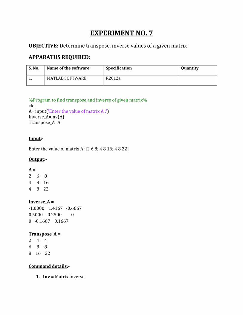
EXPERIMENT NO. 7

OBJECTIVE: Determine transpose, inverse values of a given matrix

APPARATUS REQUIRED:

S. No. Name of the software Specification Quantity

1. MATLAB SOFTWARE R2012a

%Program to find transpose and inverse of given matrix% clc A= input('Enter the value of matrix A :') Inverse_A=inv(A) Transpose_A=A'

Input:-

Enter the value of matrix A :[2 6 8; 4 8 16; 4 8 22]

Output:-

A =

2 6 8

4 8 16

4 8 22

Inverse_A =

-1.0000 1.4167 -0.6667

0.5000 -0.2500 0

0 -0.1667 0.1667

Transpose_A =

2 4 4

6 8 8

8 16 22

Command details:-

1. Inv = Matrix inverse

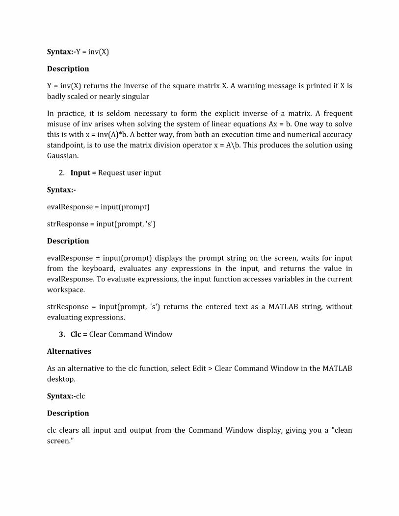
Syntax:-Y = inv(X)

Description

Y = inv(X) returns the inverse of the square matrix X. A warning message is printed if X is

badly scaled or nearly singular

In practice, it is seldom necessary to form the explicit inverse of a matrix. A frequent

misuse of inv arises when solving the system of linear equations Ax = b. One way to solve

this is with x = inv(A)*b. A better way, from both an execution time and numerical accuracy

standpoint, is to use the matrix division operator x = A\b. This produces the solution using

Gaussian.

2. Input = Request user input

Syntax:-

evalResponse = input(prompt)

strResponse = input(prompt, 's')

Description

evalResponse = input(prompt) displays the prompt string on the screen, waits for input

from the keyboard, evaluates any expressions in the input, and returns the value in

evalResponse. To evaluate expressions, the input function accesses variables in the current

workspace.

strResponse = input(prompt, 's') returns the entered text as a MATLAB string, without

evaluating expressions.

3. Clc = Clear Command Window

Alternatives

As an alternative to the clc function, select Edit > Clear Command Window in the MATLAB

desktop.

Syntax:-clc

Description

clc clears all input and output from the Command Window display, giving you a "clean

screen."

After using clc, you cannot use the scroll bar to see the history of functions, but you still can

use the up arrow to recall statements from the command history.

EXPERIMENT NO. 8

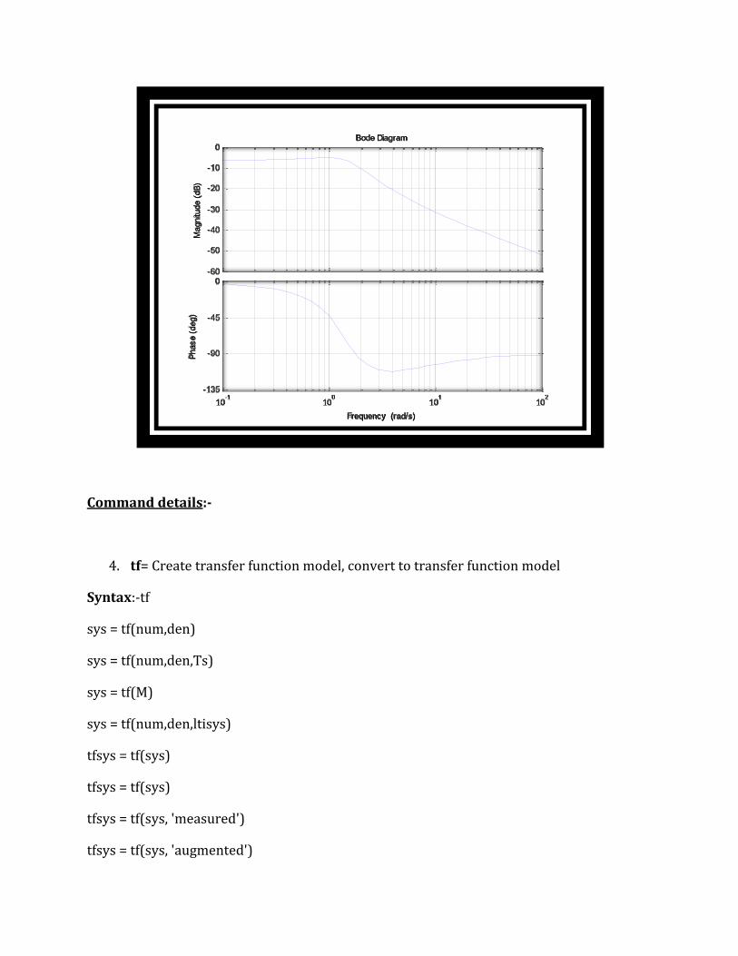
OBJECTIVE: Plot bode plot of a given transfer function.

APPARATUS REQUIRED:

S. No. Name of the software Specification Quantity

1. MATLAB SOFTWARE R2012a

%Program to find bode plot % clc num= input('Enter the value numerator :') den= input('Enter the value denominator :') fun=tf(num,den) bode(fun) gridon Input:-

Enter the value numerator :[1 4] num = 1 4 Enter the value denominator :[4 6 8] den = 4 6 8 Output:-

fun = s + 4 --------------- 4 s^2 + 6 s + 8 Continuous-time transfer function.

Command details:-

4. tf= Create transfer function model, convert to transfer function model

Syntax:-tf

sys = tf(num,den)

sys = tf(num,den,Ts)

sys = tf(M)

sys = tf(num,den,ltisys)

tfsys = tf(sys)

tfsys = tf(sys)

tfsys = tf(sys, 'measured')

tfsys = tf(sys, 'augmented')

-60

-50

-40

-30

-20

-10

0

Magnitu

de (

dB

)

10-1

100

101

102

-135

-90

-45

0

Phase (

deg)

Bode Diagram

Frequency (rad/s)

Description

Use tf to create real- or complex-valued transfer function models (TF objects) or to convert

state-space or zero-pole-gain models to transfer function form. You can also use tf to create

Generalized state-space (genss) models.

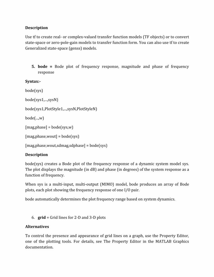
5. bode = Bode plot of frequency response, magnitude and phase of frequency

response

Syntax:-

bode(sys)

bode(sys1,...,sysN)

bode(sys1,PlotStyle1,...,sysN,PlotStyleN)

bode(...,w)

[mag,phase] = bode(sys,w)

[mag,phase,wout] = bode(sys)

[mag,phase,wout,sdmag,sdphase] = bode(sys)

Description

bode(sys) creates a Bode plot of the frequency response of a dynamic system model sys.

The plot displays the magnitude (in dB) and phase (in degrees) of the system response as a

function of frequency.

When sys is a multi-input, multi-output (MIMO) model, bode produces an array of Bode

plots, each plot showing the frequency response of one I/O pair.

bode automatically determines the plot frequency range based on system dynamics.

6. grid = Grid lines for 2-D and 3-D plots

Alternatives

To control the presence and appearance of grid lines on a graph, use the Property Editor,

one of the plotting tools. For details, see The Property Editor in the MATLAB Graphics

documentation.

Syntax

grid on

grid off

grid

grid(axes_handle,...)

grid minor

Description

The grid function turns the current axes' grid lines on and off. grid on adds major grid lines

to the current axes. grid off removes major and minor grid lines from the current axes. grid

toggles the major grid visibility state grid(axes_handle,...) uses the axes specified by

axes_handle instead of the current axes.

EXPERIMENT NO.9

OBJECTIVE: Plot bode plot of given transfer function and find gain and phase margins. APPARATUS REQUIRED:

S. No. Name of the software Specification Quantity

1. MATLAB SOFTWARE R2012a

%Program to find gain and phase margin in bode plot% clc num= input('Enter the value numerator :') den= input('Enter the value denominator :') time=0.1; h=tf([num],[den],time) bode(h) [Gm,Pm,Wgm,Wpm]=margin(h) gridon

Input:-

Enter the value numerator :[0.04 0.04]

num =

0.0400 0.0400

Enter the value denominator :[1 -1.6 0.9]

den =

1.0000 -1.6000 0.9000

Output:-

h =

0.04 z + 0.04

-----------------

z^2 - 1.6 z + 0.9

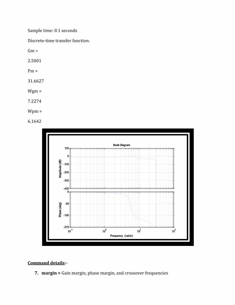
Sample time: 0.1 seconds

Discrete-time transfer function.

Gm =

2.5001

Pm =

31.6627

Wgm =

7.2274

Wpm =

6.1642

Command details:-

7. margin = Gain margin, phase margin, and crossover frequencies

-400

-300

-200

-100

0

100

Magnitu

de (

dB

)

10-1

100

101

102

-270

-180

-90

0

Phase (

deg)

Bode Diagram

Frequency (rad/s)

Syntax

[Gm,Pm,Wg,Wp] = margin(sys)

[Gm,Pm,Wg,Wp] = margin(mag,phase,w)

margin(sys)

Description

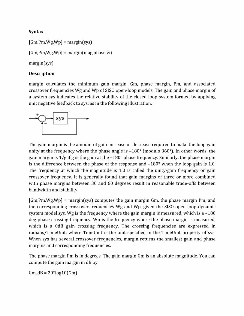
margin calculates the minimum gain margin, Gm, phase margin, Pm, and associated

crossover frequencies Wg and Wp of SISO open-loop models. The gain and phase margin of

a system sys indicates the relative stability of the closed-loop system formed by applying

unit negative feedback to sys, as in the following illustration.

The gain margin is the amount of gain increase or decrease required to make the loop gain

unity at the frequency where the phase angle is –180° (modulo 360°). In other words, the

gain margin is 1/g if g is the gain at the –180° phase frequency. Similarly, the phase margin

is the difference between the phase of the response and –180° when the loop gain is 1.0.

The frequency at which the magnitude is 1.0 is called the unity-gain frequency or gain

crossover frequency. It is generally found that gain margins of three or more combined

with phase margins between 30 and 60 degrees result in reasonable trade-offs between

bandwidth and stability.

[Gm,Pm,Wg,Wp] = margin(sys) computes the gain margin Gm, the phase margin Pm, and

the corresponding crossover frequencies Wg and Wp, given the SISO open-loop dynamic

system model sys. Wg is the frequency where the gain margin is measured, which is a –180

deg phase crossing frequency. Wp is the frequency where the phase margin is measured,

which is a 0dB gain crossing frequency. The crossing frequencies are expressed in

radians/TimeUnit, where TimeUnit is the unit specified in the TimeUnit property of sys.

When sys has several crossover frequencies, margin returns the smallest gain and phase

margins and corresponding frequencies.

The phase margin Pm is in degrees. The gain margin Gm is an absolute magnitude. You can

compute the gain margin in dB by

Gm_dB = 20*log10(Gm)

[Gm,Pm,Wg,Wp] = margin(mag,phase,w) derives the gain and phase margins from Bode

frequency response data (magnitude, phase, and frequency vector). margin interpolates

between the frequency points to estimate the margin values. Provide the gain data mag in

absolute units, and phase data phase in degrees. You can provide the frequency vector w in

any units; margin returns crossover frequencies wg and wg in the same units.

margin(sys), without output arguments, plots the Bode response of sys on the screen and

indicates the gain and phase margins on the plot. By default, gain margins are expressed in

dB on the plot.

EXPERIMENT NO. 10

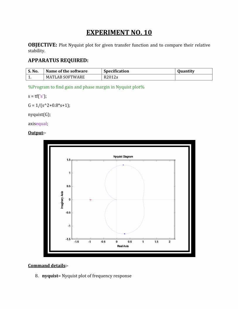
OBJECTIVE: Plot Nyquist plot for given transfer function and to compare their relative stability.

APPARATUS REQUIRED:

S. No. Name of the software Specification Quantity

1. MATLAB SOFTWARE R2012a

%Program to find gain and phase margin in Nyquist plot%

s = tf('s');

G = 1/(s^2+0.8*s+1);

nyquist(G);

axisequal;

Output:-

Command details:-

8. nyquist= Nyquist plot of frequency response

-1.5 -1 -0.5 0 0.5 1 1.5 2-1.5

-1

-0.5

0

0.5

1

1.5

Nyquist Diagram

Real Axis

Imagin

ary

Axis

Syntax:-

nyquist(sys)

nyquist(sys,w)

nyquist(sys1,sys2,...,sysN)

nyquist(sys1,sys2,...,sysN,w)

[re,im,w,sdre,sdim] = nyquist(sys)

Description

nyquist creates a Nyquist plot of the frequency response of a dynamic system model. When

invoked without left-hand arguments, nyquist produces a Nyquist plot on the screen.

Nyquist plots are used to analyze system properties including gain margin, phase margin,

and stability.

nyquist(sys) creates a Nyquist plot of a dynamic system sys. This model can be continuous

or discrete, and SISO or MIMO. In the MIMO case, nyquist produces an array of Nyquist

plots, each plot showing the response of one particular I/O channel. The frequency points

are chosen automatically based on the system poles and zeros.

nyquist(sys,w) explicitly specifies the frequency range or frequency points to be used for

the plot. To focus on a particular frequency interval, set w = {wmin,wmax}. To use

particular frequency points, set w to the vector of desired frequencies. Use logspace to

generate logarithmically spaced frequency vectors. Frequencies must be in rad/TimeUnit,

where TimeUnit is the time units of the input dynamic system, specified in the TimeUnit

property of sys.

nyquist(sys1,sys2,...,sysN) or nyquist(sys1,sys2,...,sysN,w) superimposes the Nyquist plots

of several LTI models on a single figure. All systems must have the same number of inputs

and outputs, but may otherwise be a mix of continuous- and discrete-time systems. You can

also specify a distinctive color, linestyle, and/or marker for each system plot with the

syntax

nyquist(sys1,'PlotStyle1',...,sysN,'PlotStyleN')

See bode for an example.

When invoked with left-hand arguments

[re,im,w] = nyquist(sys)

[re,im] = nyquist(sys,w)

return the real and imaginary parts of the frequency response at the frequencies w (in

rad/TimeUnit). re and im are 3-D arrays (see "Arguments" below for details).0

………………………………………………………………………………..

[re,im,w,sdre,sdim] = nyquist(sys) also returns the standard deviations of re and im for the

identified system sys.

EXPERIMENT NO. 11

OBJECTIVE: PLOT UNIT STEP RESPONSEOF GIVEN TRANSFER FUNCTION

AND FIND PEAK OVERSHOOT, PEAK TIME.

APPARATUS REQUIRED:

S. No. Name of the software Specification Quantity

1. MATLAB SOFTWARE R2012a

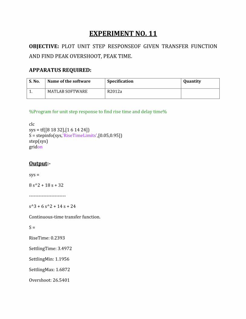
%Program for unit step response to find rise time and delay time%

clc sys = tf([8 18 32],[1 6 14 24]) S = stepinfo(sys,'RiseTimeLimits',[0.05,0.95]) step(sys) gridon

Output:-

sys =

8 s^2 + 18 s + 32

-----------------------

s^3 + 6 s^2 + 14 s + 24

Continuous-time transfer function.

S =

RiseTime: 0.2393

SettlingTime: 3.4972

SettlingMin: 1.1956

SettlingMax: 1.6872

Overshoot: 26.5401

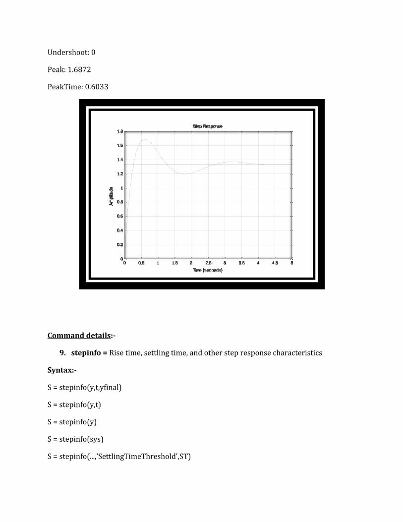
Undershoot: 0

Peak: 1.6872

PeakTime: 0.6033

Command details:-

9. stepinfo = Rise time, settling time, and other step response characteristics

Syntax:-

S = stepinfo(y,t,yfinal)

S = stepinfo(y,t)

S = stepinfo(y)

S = stepinfo(sys)

S = stepinfo(...,'SettlingTimeThreshold',ST)

0 0.5 1 1.5 2 2.5 3 3.5 4 4.5 50

0.2

0.4

0.6

0.8

1

1.2

1.4

1.6

1.8

Step Response

Time (seconds)

Am

plit

ude

S = stepinfo(...,'RiseTimeLimits',RT)

Description

S = stepinfo(y,t,yfinal) takes step response data (t,y) and a steady-state value yfinal and

returns a structure S containing the following performance indicators:

RiseTime — Rise time

SettlingTime — Settling time

SettlingMin — Minimum value of y once the response has risen

SettlingMax — Maximum value of y once the response has risen

Overshoot — Percentage overshoot (relative to yfinal)

Undershoot — Percentage undershoot

Peak — Peak absolute value of y

PeakTime — Time at which this peak is reached

For SISO responses, t and y are vectors with the same length NS. For systems with NU

inputs and NY outputs, you can specify y as an NS-by-NY-by-NU array (see step) and yfinal

as an NY-by-NU array. stepinfo then returns a NY-by-NU structure array S of performance

metrics for each I/O pair.

S = stepinfo(y,t) uses the last sample value of y as steady-state value yfinal. S = stepinfo(y)

assumes t = 1:ns.

S = stepinfo(sys)computes the step response characteristics for an LTI model sys (see tf,

zpk, or ss for details).

S = stepinfo(...,'SettlingTimeThreshold',ST) lets you specify the threshold ST used in the

settling time calculation. The response has settled when the error |y(t) - yfinal| becomes

smaller than a fraction ST of its peak value. The default value is ST=0.02 (2%).

S = stepinfo(...,'RiseTimeLimits',RT) lets you specify the lower and upper thresholds used in

the rise time calculation. By default, the rise time is the time the response takes to rise from

10 to 90% of the steady-state value (RT=[0.1 0.9]). Note that RT(2) is also used to calculate

SettlingMin and SettlingMax.

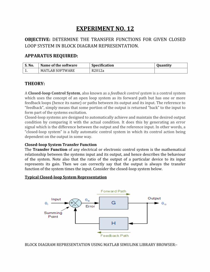
EXPERIMENT NO. 12

OBJECTIVE: DETERMINE THE TRANSFER FUNCTIONS FOR GIVEN CLOSED

LOOP SYSTEM IN BLOCK DIAGRAM REPRESENTATION.

APPARATUS REQUIRED:

S. No. Name of the software Specification Quantity

1. MATLAB SOFTWARE R2012a

THEORY:

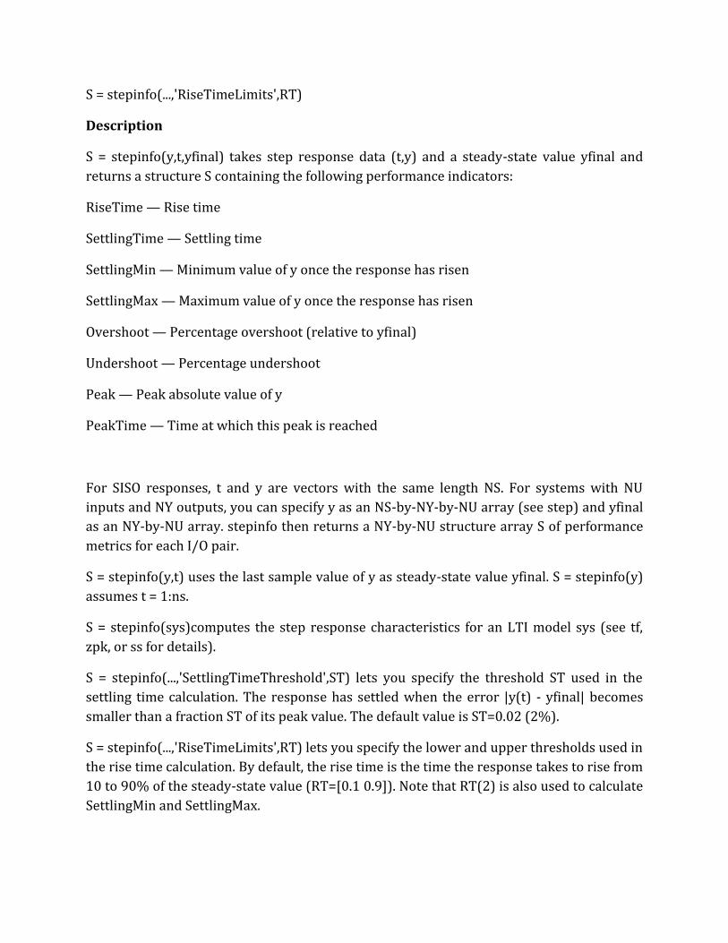
A Closed-loop Control System, also known as a feedback control system is a control system which uses the concept of an open loop system as its forward path but has one or more feedback loops (hence its name) or paths between its output and its input. The reference to “feedback”, simply means that some portion of the output is returned “back” to the input to form part of the systems excitation. Closed-loop systems are designed to automatically achieve and maintain the desired output condition by comparing it with the actual condition. It does this by generating an error signal which is the difference between the output and the reference input. In other words, a “closed-loop system” is a fully automatic control system in which its control action being dependent on the output in some way.

Closed-loop System Transfer Function The Transfer Function of any electrical or electronic control system is the mathematical relationship between the systems input and its output, and hence describes the behaviour of the system. Note also that the ratio of the output of a particular device to its input represents its gain. Then we can correctly say that the output is always the transfer function of the system times the input. Consider the closed-loop system below.

Typical Closed-loop System Representation

BLOCK DIAGRAM REPRESENTATION USING MATLAB SIMULINK LIBRARY BROWSER:-

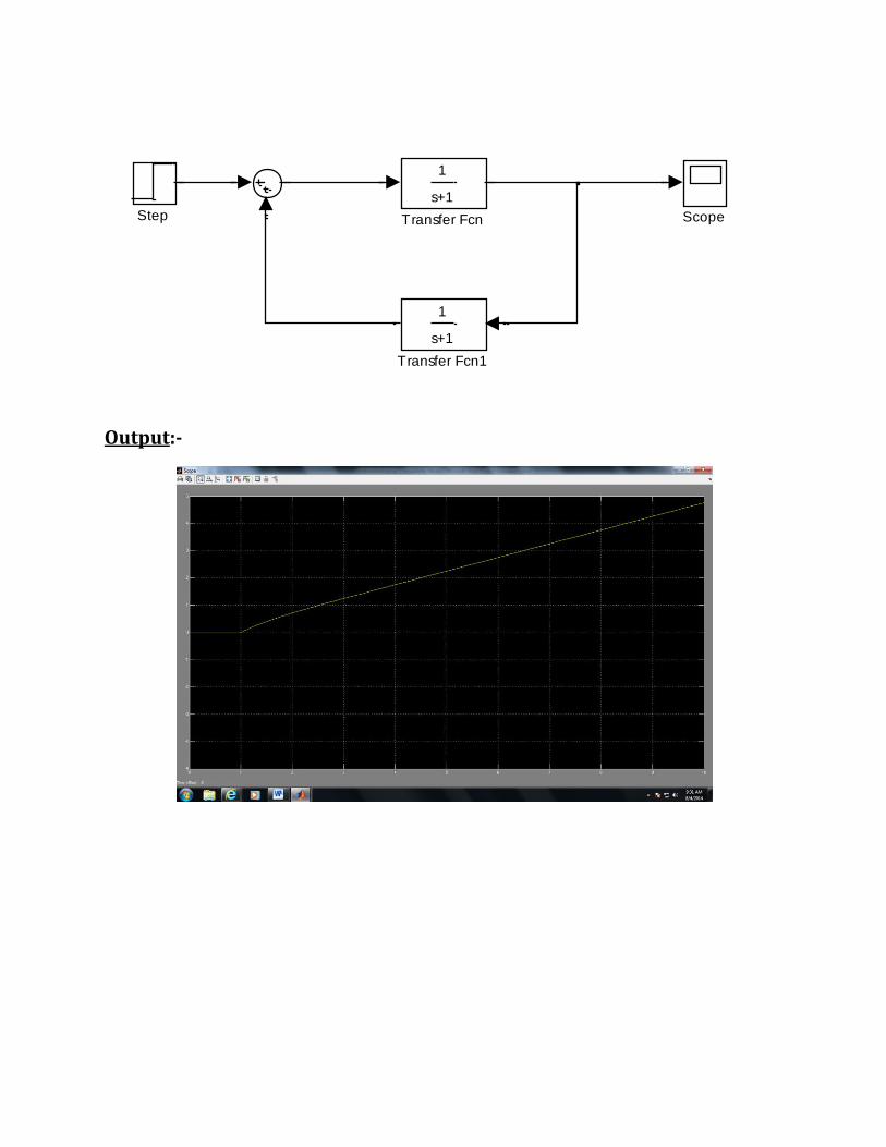
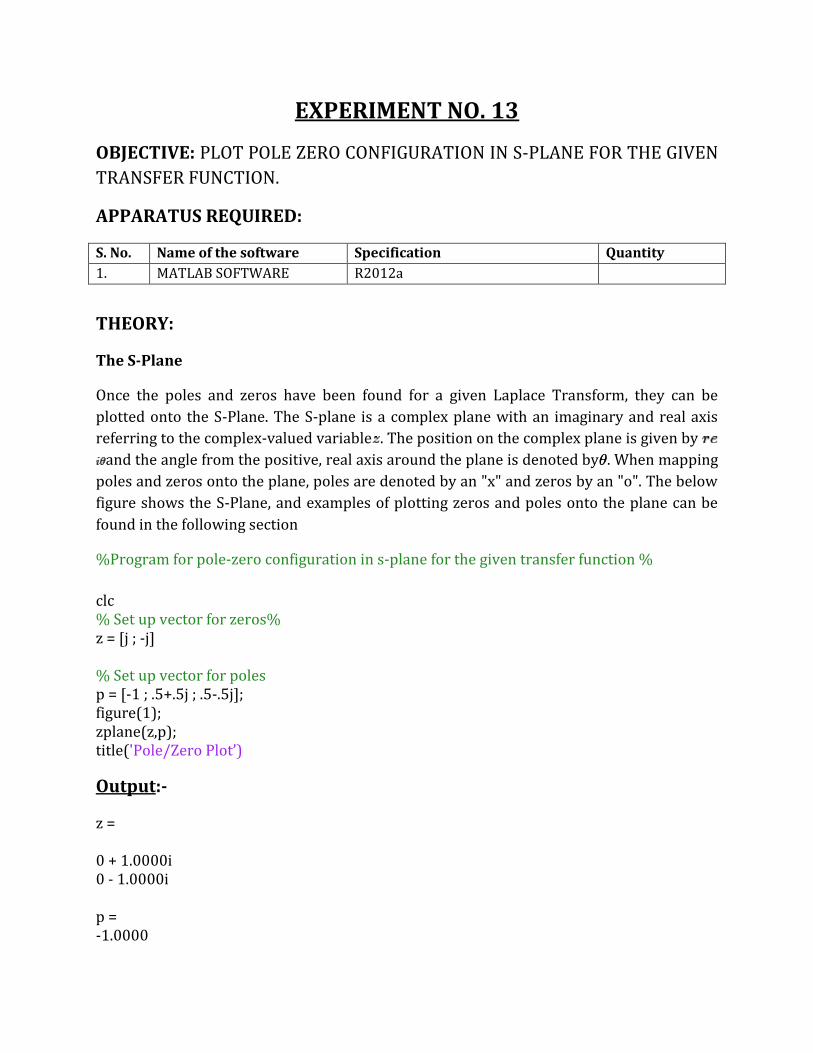
Output:-

1

s+1

Transfer Fcn1

1

s+1

Transfer FcnStep Scope

EXPERIMENT NO. 13

OBJECTIVE: PLOT POLE ZERO CONFIGURATION IN S-PLANE FOR THE GIVEN

TRANSFER FUNCTION.

APPARATUS REQUIRED:

S. No. Name of the software Specification Quantity

1. MATLAB SOFTWARE R2012a

THEORY:

The S-Plane

Once the poles and zeros have been found for a given Laplace Transform, they can be

plotted onto the S-Plane. The S-plane is a complex plane with an imaginary and real axis

referring to the complex-valued variable . The position on the complex plane is given by

and the angle from the positive, real axis around the plane is denoted by . When mapping

poles and zeros onto the plane, poles are denoted by an "x" and zeros by an "o". The below

figure shows the S-Plane, and examples of plotting zeros and poles onto the plane can be

found in the following section

%Program for pole-zero configuration in s-plane for the given transfer function %

clc % Set up vector for zeros% z = [j ; -j] % Set up vector for poles p = [-1 ; .5+.5j ; .5-.5j]; figure(1); zplane(z,p); title('Pole/Zero Plot’)

Output:-

z = 0 + 1.0000i 0 - 1.0000i p = -1.0000

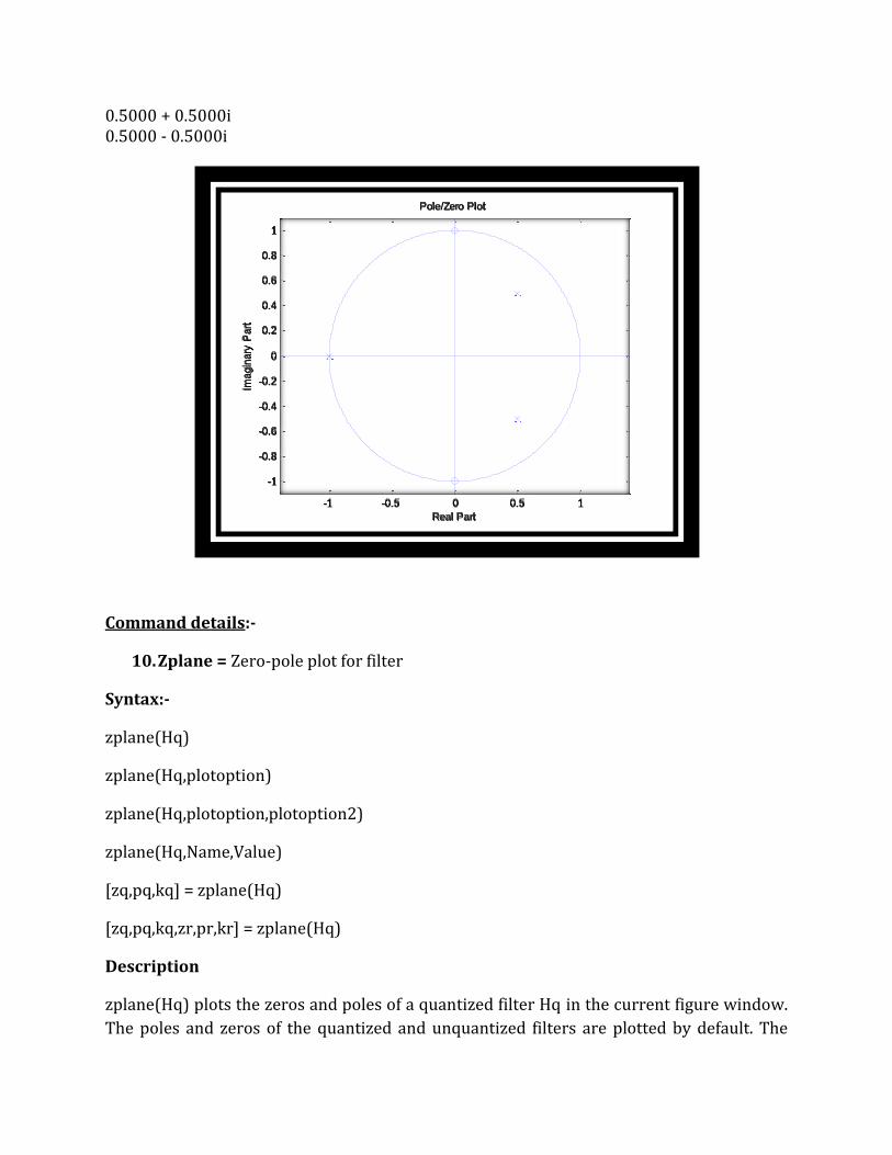
0.5000 + 0.5000i 0.5000 - 0.5000i

Command details:-

10. Zplane = Zero-pole plot for filter

Syntax:-

zplane(Hq)

zplane(Hq,plotoption)

zplane(Hq,plotoption,plotoption2)

zplane(Hq,Name,Value)

[zq,pq,kq] = zplane(Hq)

[zq,pq,kq,zr,pr,kr] = zplane(Hq)

Description

zplane(Hq) plots the zeros and poles of a quantized filter Hq in the current figure window.

The poles and zeros of the quantized and unquantized filters are plotted by default. The

-1 -0.5 0 0.5 1

-1

-0.8

-0.6

-0.4

-0.2

0

0.2

0.4

0.6

0.8

1

Real Part

Imagin

ary

Part

Pole/Zero Plot

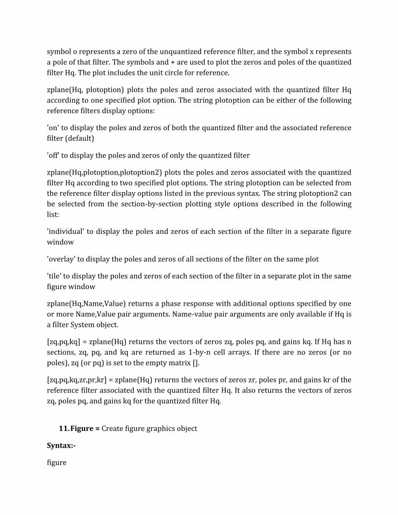
symbol o represents a zero of the unquantized reference filter, and the symbol x represents

a pole of that filter. The symbols and + are used to plot the zeros and poles of the quantized

filter Hq. The plot includes the unit circle for reference.

zplane(Hq, plotoption) plots the poles and zeros associated with the quantized filter Hq

according to one specified plot option. The string plotoption can be either of the following

reference filters display options:

'on' to display the poles and zeros of both the quantized filter and the associated reference

filter (default)

'off' to display the poles and zeros of only the quantized filter

zplane(Hq,plotoption,plotoption2) plots the poles and zeros associated with the quantized

filter Hq according to two specified plot options. The string plotoption can be selected from

the reference filter display options listed in the previous syntax. The string plotoption2 can

be selected from the section-by-section plotting style options described in the following

list:

'individual' to display the poles and zeros of each section of the filter in a separate figure

window

'overlay' to display the poles and zeros of all sections of the filter on the same plot

'tile' to display the poles and zeros of each section of the filter in a separate plot in the same

figure window

zplane(Hq,Name,Value) returns a phase response with additional options specified by one

or more Name,Value pair arguments. Name-value pair arguments are only available if Hq is

a filter System object.

[zq,pq,kq] = zplane(Hq) returns the vectors of zeros zq, poles pq, and gains kq. If Hq has n

sections, zq, pq, and kq are returned as 1-by-n cell arrays. If there are no zeros (or no

poles), zq (or pq) is set to the empty matrix [].

[zq,pq,kq,zr,pr,kr] = zplane(Hq) returns the vectors of zeros zr, poles pr, and gains kr of the

reference filter associated with the quantized filter Hq. It also returns the vectors of zeros

zq, poles pq, and gains kq for the quantized filter Hq.

11. Figure = Create figure graphics object

Syntax:-

figure

figure('PropertyName',propertyvalue,...)

figure(h)

h = figure(...)

Properties

For a list of properties, see Figure Properties.

Description

figure creates figure graphics objects. Figure objects are the individual windows on the

screen in which the MATLAB software displays graphical output.

figure creates a new figure object using default property values. This automatically

becomes the current figure and raises it above all other figures on the screen until a new

figure is either created or called.

figure('PropertyName',propertyvalue,...) creates a new figure object using the values of the

properties specified. For a description of the properties, see Figure Properties. MATLAB

uses default values for any properties that you do not explicitly define as arguments.

figure(h) does one of two things, depending on whether or not a figure with handle h exists.

If h is the handle to an existing figure, figure(h) makes the figure identified by h the current

figure, makes it visible, and raises it above all other figures on the screen. The current

figure is the target for graphics output. If h is not the handle to an existing figure, but is an

integer, figure(h) creates a figure and assigns it the handle h. figure(h) where h is not the

handle to a figure, and is not an integer, is an error.

h = figure(...) returns the handle to the figure object.

EXPERIMENT NO. 14

OBJECTIVE: PLOT THE NYQUIST PLOT FOR GIVEN TRANSFER FUNCTION

AND TO DISCUSS STABILITY, GAIN AND PHSE MARGIN

APPARATUS REQUIRED:

S. No. Name of the software Specification Quantity

1. MATLAB SOFTWARE R2012a

THEORY:

The Nyquist plot of a transfer function, usually the loop transfer function GH(z), is a mapping of Nyquist contour in z-plane onto GH(z)plane which is in polar coordinates. Thus it is sometimes known as polar plot. Absolute and relative stabilities can be determined from the Nyquist plot using Nyquist stability criterion. Given the loop transfer function

GH(z)of a digital control system, the polar plot of GH(z)is obtained by setting z= ejωT and

varying ω from 0 to ∞.

Nyquist stability criterion: The closed loop transfer function of single input single output digital control system is described by M(z) = GH(z)/ 1+ GH(z)

Characteristic equation 1+ GH(z)=0

The stability of the system depends on the roots of the characteristic equation or poles of the system. All the roots of the characteristic equation must lie inside the unit circle for the system to be stable.

%Program to plot the Nyquist plot for given transfer function and to discuss closed loop

stability, gain and phase margin. %

clc

num= input('Enter the value numerator :')

den= input('Enter the value denominator :')

time=0.1;

h=tf([num],[den],time)

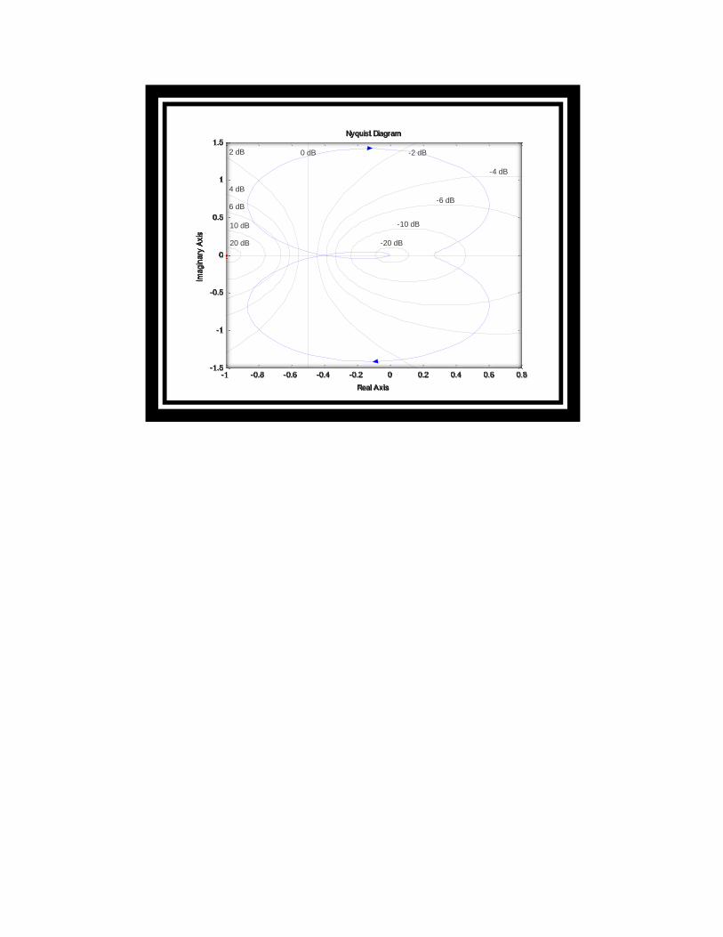
nyquist(h)

[Gm,Pm,Wgm,Wpm]=margin(h)

gridon

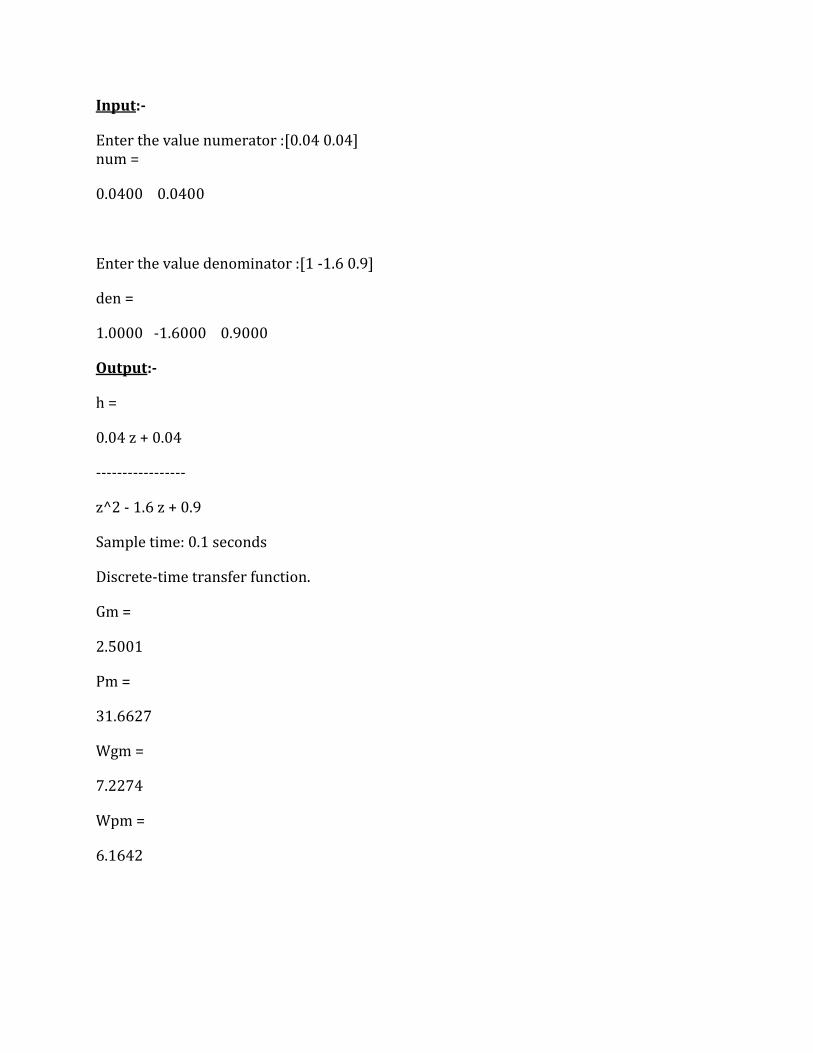
Input:-

Enter the value numerator :[0.04 0.04] num =

0.0400 0.0400

Enter the value denominator :[1 -1.6 0.9]

den =

1.0000 -1.6000 0.9000

Output:-

h =

0.04 z + 0.04

-----------------

z^2 - 1.6 z + 0.9

Sample time: 0.1 seconds

Discrete-time transfer function.

Gm =

2.5001

Pm =

31.6627

Wgm =

7.2274

Wpm =

6.1642

-1 -0.8 -0.6 -0.4 -0.2 0 0.2 0.4 0.6 0.8-1.5

-1

-0.5

0

0.5

1

1.5

0 dB

-20 dB

-10 dB

-6 dB

-4 dB

-2 dB

20 dB

10 dB

6 dB

4 dB

2 dB

Nyquist Diagram

Real Axis

Imagin

ary

Axis