PAMM · Proc. Appl. Math. Mech. 13, 433 – 434 (2013) / DOI 10.1002/pamm.201310211

Convergence of a Finite Difference Scheme for a Parabolic TransmissionProblem in Disjoint Domains

Zorica Milovanovic1,∗

1 University of Belgrade, Faculty of Mathematics, Studentski trg 16, 11000 Belgrade, Serbia

In this paper we investigate a parabolic transmission problem in disjoint domains. An a priori estimate for its weak solution inappropriate Sobolev-like space is proved. The convergence of a finite difference scheme (FDS) approximating this problemis analyzed.

c© 2013 Wiley-VCH Verlag GmbH & Co. KGaA, Weinheim

1 Introduction

Mathematical models of energy and mass transfer in domains with layers lead to so called transmission problems. In thispaper we consider a non-standard parabolic transmission problems in disjoint domains. As a model example it is taken an areaconsisting of two non-adjacent rectangles. In each subarea was given an initial-boundary problem of parabolic type, wherethe interaction between their solutions is described by nonlocal integral conjugation conditions. Similar problem with moresimple geometry was considered in [2].

2 Formulation of the problem and its approximation

As a model example, we consider the following initial-boundary-value problem (IBVP) :

∂ui∂t− ∂

∂x

(pi(x, y)

∂ui∂x

)− ∂

∂y

(qi(x, y)

∂ui∂y

)+ri(x, y)ui = fi(x, y, t), (x, y) ∈ (ai, bi)×(ci, di), t > 0, i = 1, 2 (1)

with the initial conditions ui(x, y, 0) = ui0(x, y), (x, y) ∈ (ai, bi)× (ci, di), the external Dirichlet boundary conditions

u1(a1, y, t) = 0, y ∈ (c1, d1), u2(x, c2, t) = u2(x, d2, t) = 0, x ∈ (a2, b2), u2(b2, y, t) = 0, y ∈ (c2, d2), (2)

and the internal conjugation conditions of non-local Robin-Dirichlet type

p1(b1, y)∂u1∂x

(b1, y, t) + α1(y)u1(b1, y, t) =

∫ d2

c2

β1(y, y′)u2(a2, y′, t) dy′, y ∈ (c1, d1), (3)

(−p2

∂u2∂x

+ α2u2

) ∣∣∣∣x=a2

=

∫ d1c1β2(y, y′)u1(b1, y

′, t)dy′ +∫ b1a1β2(y, x′)u1(x′, c1, t)dx

′, y ∈ (c2, c1),∫ d1c1β2(y, y′)u1(b1, y

′, t)dy′, y ∈ (c1, d1),∫ d1c1β2(y, y′)u1(b1, y

′, t)dy′ +∫ b1a1β2(y, x′)u1(x′, d1, t)dx

′, y ∈ (d1, d2),

(4)

−q1(x, c1)∂u1∂y

(x, c1, t) + α1(x)u1(x, c1, t) =

∫ c1

c2

β1(x, y′)u2(a2, y′, t) dy′, x ∈ (a1, b1), (5)

q1(x, d1)∂u1∂y

(x, d1, t) + α1(x)u1(x, d1, t) =

∫ d2

d1

β1(x, y′)u2(a2, y′, t) dy′, x ∈ (a1, b1). (6)

If we assume that the input data satisfy the usual regularity and ellipticity conditions the initial-boundary-value problem (1)-(6)has a unique weak solution u ∈W (0, T ), and this depends continuously on f = (f1, f2) and u0 = (u10, u20) (comp. [2], [5]).

Let ωi,hi be a uniform mesh in [ai, bi] with step size hi, ωi,ki – a uniform mesh in [ci, di] with the step size ki and ωτ –a uniform mesh in [0, T ]with step size τ . Keeping denotations from [2] we approximate the initial-boundary-value problem(1)-(6) with the following explicit finite difference scheme (see [3], [4]):

v1,t − (p1v1,x)x − (q1v1,y)y + r1v1 = f1, x ∈ ω1,h1 , y ∈ ω1,k1 , t ∈ ω−τ ,

v1,t(b1, y, t) +2

h1

[(p1(b1, y)v1,x(b1, y, t)) + α1(y)v1(b1, y, t)− k2

∑y′∈ω2,k2

β1(y, y′)v2(a2, y′, t)]

−(q1v1,y)y(b1, y, t) + r1(b1, y)v1(b1, y, t) = f1(b1, y, t), y ∈ ω1,k1 , t ∈ ω−τ ,

∗ Corresponding author: e-mail zorica.milovanovic@gmail.com

c© 2013 Wiley-VCH Verlag GmbH & Co. KGaA, Weinheim

434 Section 18: Numerical methods of differential equations

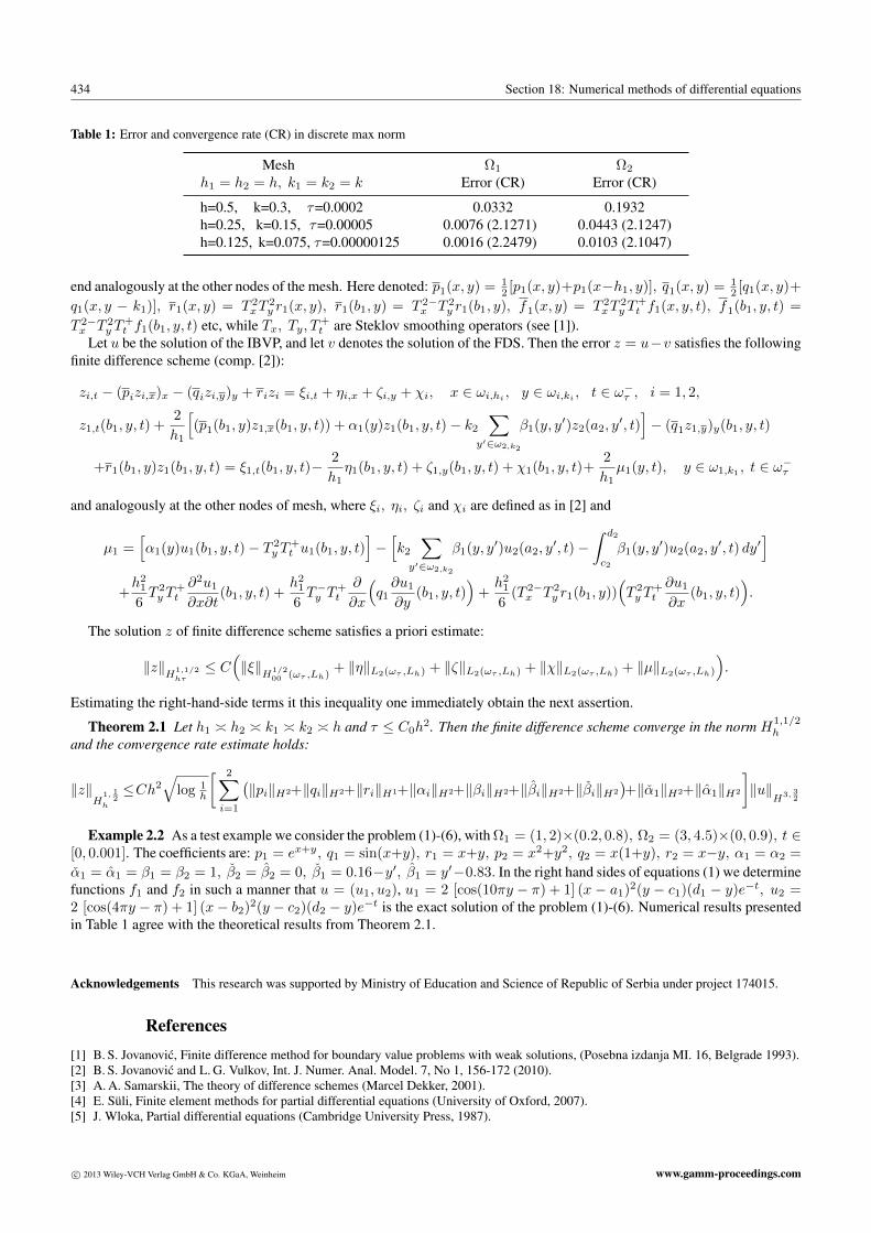
Table 1: Error and convergence rate (CR) in discrete max norm

Mesh Ω1 Ω2

h1 = h2 = h, k1 = k2 = k Error (CR) Error (CR)

h=0.5, k=0.3, τ=0.0002 0.0332 0.1932h=0.25, k=0.15, τ=0.00005 0.0076 (2.1271) 0.0443 (2.1247)h=0.125, k=0.075, τ=0.00000125 0.0016 (2.2479) 0.0103 (2.1047)

end analogously at the other nodes of the mesh. Here denoted: p1(x, y) = 12 [p1(x, y)+p1(x−h1, y)], q1(x, y) = 1

2 [q1(x, y)+

q1(x, y − k1)], r1(x, y) = T 2xT

2y r1(x, y), r1(b1, y) = T 2−

x T 2y r1(b1, y), f1(x, y) = T 2

xT2y T

+t f1(x, y, t), f1(b1, y, t) =

T 2−x T 2

y T+t f1(b1, y, t) etc, while Tx, Ty, T+

t are Steklov smoothing operators (see [1]).Let u be the solution of the IBVP, and let v denotes the solution of the FDS. Then the error z = u−v satisfies the following

finite difference scheme (comp. [2]):

zi,t − (pizi,x)x − (qizi,y)y + rizi = ξi,t + ηi,x + ζi,y + χi, x ∈ ωi,hi , y ∈ ωi,ki , t ∈ ω−τ , i = 1, 2,

z1,t(b1, y, t) +2

h1

[(p1(b1, y)z1,x(b1, y, t)) + α1(y)z1(b1, y, t)− k2

∑y′∈ω2,k2

β1(y, y′)z2(a2, y′, t)]− (q1z1,y)y(b1, y, t)

+r1(b1, y)z1(b1, y, t) = ξ1,t(b1, y, t)−2

h1η1(b1, y, t) + ζ1,y(b1, y, t) + χ1(b1, y, t)+

2

h1µ1(y, t), y ∈ ω1,k1 , t ∈ ω−τ

and analogously at the other nodes of mesh, where ξi, ηi, ζi and χi are defined as in [2] and

µ1 =[α1(y)u1(b1, y, t)− T 2

y T+t u1(b1, y, t)

]−[k2

∑y′∈ω2,k2

β1(y, y′)u2(a2, y′, t)−

∫ d2

c2

β1(y, y′)u2(a2, y′, t) dy′

]+h216T 2y T

+t

∂2u1∂x∂t

(b1, y, t) +h216T−y T

+t

∂

∂x

(q1∂u1∂y

(b1, y, t))

+h216

(T 2−x T 2

y r1(b1, y))(T 2y T

+t

∂u1∂x

(b1, y, t)).

The solution z of finite difference scheme satisfies a priori estimate:

‖z‖H

1,1/2hτ

≤ C(‖ξ‖

H1/200 (ωτ ,Lh)

+ ‖η‖L2(ωτ ,Lh) + ‖ζ‖L2(ωτ ,Lh) + ‖χ‖L2(ωτ ,Lh) + ‖µ‖L2(ωτ ,Lh)

).

Estimating the right-hand-side terms it this inequality one immediately obtain the next assertion.

Theorem 2.1 Let h1 h2 k1 k2 h and τ ≤ C0h2. Then the finite difference scheme converge in the norm H

1,1/2h

and the convergence rate estimate holds:

‖z‖H

1, 12

h

≤Ch2√

log 1h

[ 2∑i=1

(‖pi‖H2+‖qi‖H2+‖ri‖H1+‖αi‖H2+‖βi‖H2+‖βi‖H2+‖βi‖H2

)+‖α1‖H2+‖α1‖H2

]‖u‖

H3, 32

Example 2.2 As a test example we consider the problem (1)-(6), with Ω1 = (1, 2)×(0.2, 0.8), Ω2 = (3, 4.5)×(0, 0.9), t ∈[0, 0.001]. The coefficients are: p1 = ex+y, q1 = sin(x+y), r1 = x+y, p2 = x2+y2, q2 = x(1+y), r2 = x−y, α1 = α2 =

α1 = α1 = β1 = β2 = 1, β2 = β2 = 0, β1 = 0.16−y′, β1 = y′−0.83. In the right hand sides of equations (1) we determinefunctions f1 and f2 in such a manner that u = (u1, u2), u1 = 2 [cos(10πy − π) + 1] (x − a1)2(y − c1)(d1 − y)e−t, u2 =2 [cos(4πy − π) + 1] (x− b2)2(y − c2)(d2 − y)e−t is the exact solution of the problem (1)-(6). Numerical results presentedin Table 1 agree with the theoretical results from Theorem 2.1.

Acknowledgements This research was supported by Ministry of Education and Science of Republic of Serbia under project 174015.

References[1] B. S. Jovanovic, Finite difference method for boundary value problems with weak solutions, (Posebna izdanja MI. 16, Belgrade 1993).[2] B. S. Jovanovic and L. G. Vulkov, Int. J. Numer. Anal. Model. 7, No 1, 156-172 (2010).[3] A. A. Samarskii, The theory of difference schemes (Marcel Dekker, 2001).[4] E. Süli, Finite element methods for partial differential equations (University of Oxford, 2007).[5] J. Wloka, Partial differential equations (Cambridge University Press, 1987).

c© 2013 Wiley-VCH Verlag GmbH & Co. KGaA, Weinheim www.gamm-proceedings.com