Convex Optimization M2 - École Normale Supérieureaspremon/PDF/MVA/UnconstrainedEquality.pdfConvex Optimization M2. 5/53. Strong convexity and implications fis strongly convex on

Convex Optimization M2

Lecture 4

A. d’Aspremont. Convex Optimization M2. 1/53

Unconstrained minimization



� terminology and assumptions

� gradient descent method

� steepest descent method

� Newton’s method

� self-concordant functions

� implementation



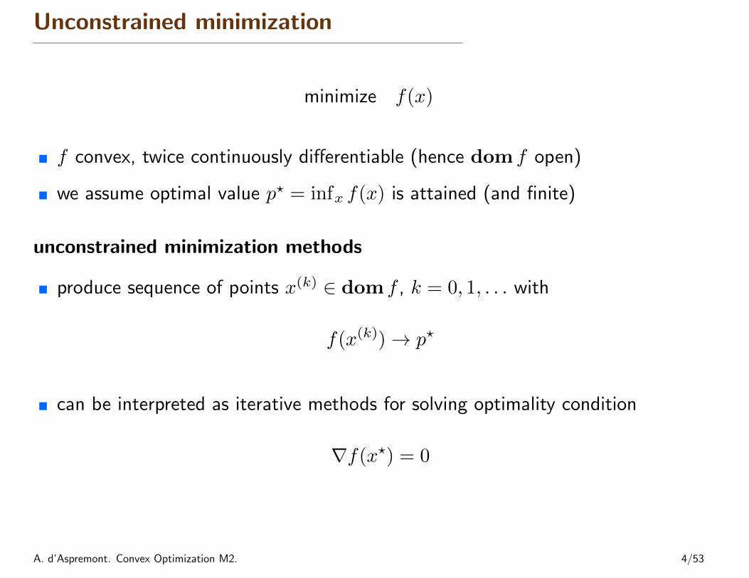
minimize f(x)

� f convex, twice continuously differentiable (hence dom f open)

� we assume optimal value p? = infx f(x) is attained (and finite)

unconstrained minimization methods

� produce sequence of points x(k) ∈ dom f , k = 0, 1, . . . with

f(x(k))→ p?

� can be interpreted as iterative methods for solving optimality condition

∇f(x?) = 0


Initial point and sublevel set

algorithms in this chapter require a starting point x(0) such that

� x(0) ∈ dom f

� sublevel set S = {x | f(x) ≤ f(x(0))} is closed

2nd condition is hard to verify, except when all sublevel sets are closed:

� equivalent to condition that epi f is closed

� true if dom f = Rn

� true if f(x)→∞ as x→ bddom f

examples of differentiable functions with closed sublevel sets:

f(x) = log(

m∑i=1

exp(aTi x+ bi)), f(x) = −m∑i=1

log(bi − aTi x)


Strong convexity and implications

f is strongly convex on S if there exists an m > 0 such that

∇2f(x) � mI for all x ∈ S

implications

� for x, y ∈ S,

f(y) ≥ f(x) +∇f(x)T (y − x) +m

2‖x− y‖22

hence, S is bounded

� p? > −∞, and for x ∈ S,

f(x)− p? ≤ 1

2m‖∇f(x)‖22

useful as stopping criterion (if you know m)


Descent methods

x(k+1) = x(k) + t(k)∆x(k) with f(x(k+1)) < f(x(k))

� other notations: x+ = x+ t∆x, x := x+ t∆x

� ∆x is the step, or search direction; t is the step size, or step length

� from convexity, f(x+) < f(x) implies ∇f(x)T∆x < 0(i.e., ∆x is a descent direction)

General descent method.

given a starting point x ∈ dom f .repeat

1. Determine a descent direction ∆x.2. Line search. Choose a step size t > 0.3. Update. x := x+ t∆x.

until stopping criterion is satisfied.


Line search types

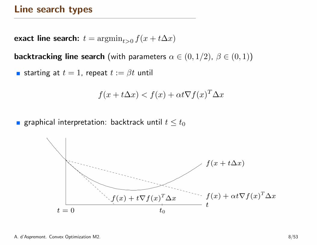
exact line search: t = argmint>0 f(x+ t∆x)

backtracking line search (with parameters α ∈ (0, 1/2), β ∈ (0, 1))

� starting at t = 1, repeat t := βt until

f(x+ t∆x) < f(x) + αt∇f(x)T∆x

� graphical interpretation: backtrack until t ≤ t0

t

f(x + t∆x)

t = 0 t0

f(x) + αt∇f(x)T∆xf(x) + t∇f(x)T∆x


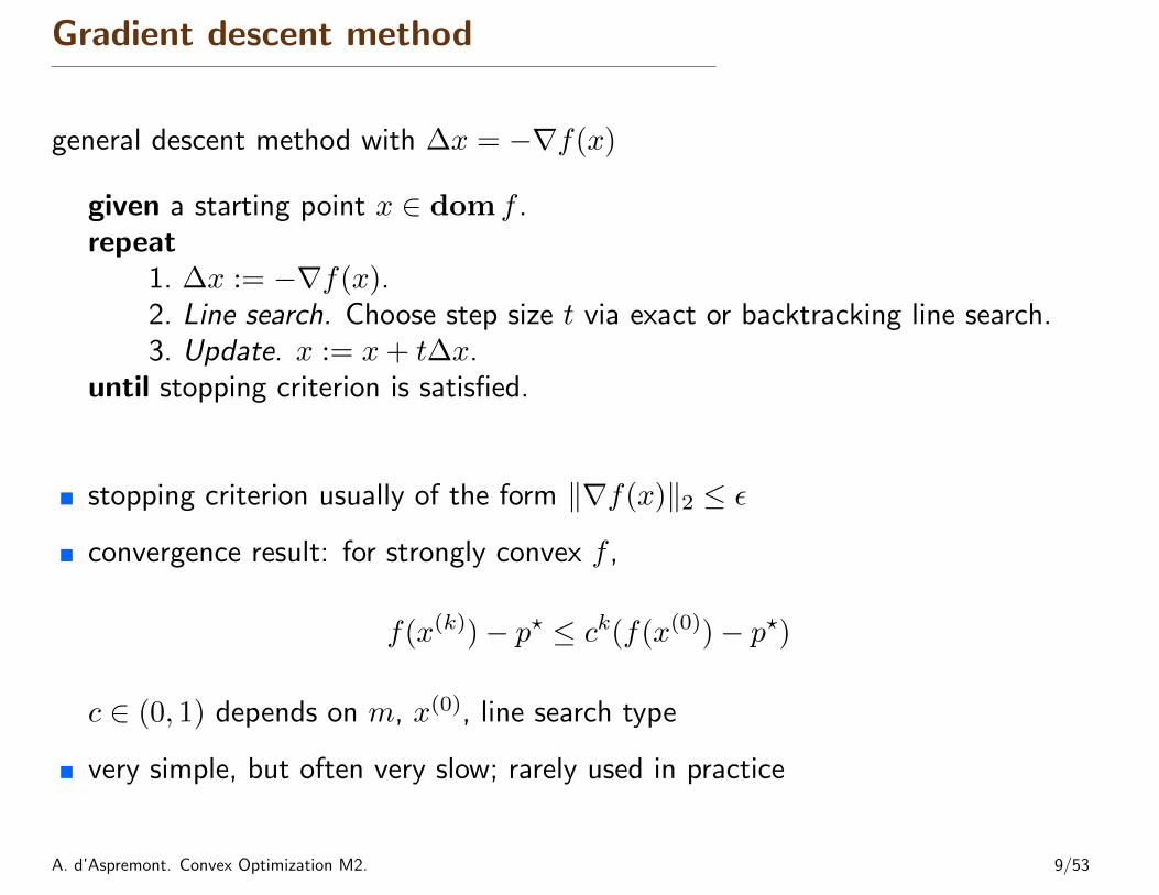
Gradient descent method

general descent method with ∆x = −∇f(x)

given a starting point x ∈ dom f .repeat

1. ∆x := −∇f(x).2. Line search. Choose step size t via exact or backtracking line search.3. Update. x := x+ t∆x.

until stopping criterion is satisfied.

� stopping criterion usually of the form ‖∇f(x)‖2 ≤ ε

� convergence result: for strongly convex f ,

f(x(k))− p? ≤ ck(f(x(0))− p?)

c ∈ (0, 1) depends on m, x(0), line search type

� very simple, but often very slow; rarely used in practice


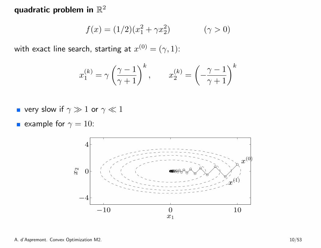
quadratic problem in R2

f(x) = (1/2)(x21 + γx22) (γ > 0)

with exact line search, starting at x(0) = (γ, 1):

x(k)1 = γ

(γ − 1

γ + 1

)k

, x(k)2 =

(−γ − 1

γ + 1

)k

� very slow if γ � 1 or γ � 1

� example for γ = 10:

x1

x2

x(0)

x(1)

−10 0 10

−4

0

4


nonquadratic example

f(x1, x2) = ex1+3x2−0.1 + ex1−3x2−0.1 + e−x1−0.1

x(0)

x(1)

x(2)

x(0)

x(1)

backtracking line search exact line search


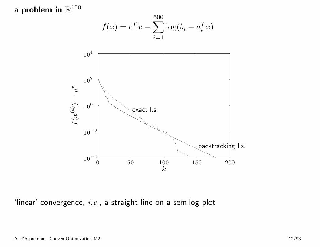
a problem in R100

f(x) = cTx−500∑i=1

log(bi − aTi x)

k

f(x

(k) )

−p⋆

exact l.s.

backtracking l.s.

0 50 100 150 20010−4

10−2

100

102

104

‘linear’ convergence, i.e., a straight line on a semilog plot


Steepest descent method

normalized steepest descent direction (at x, for norm ‖ · ‖):

∆xnsd = argmin{∇f(x)Tv | ‖v‖ = 1}

interpretation: for small v, f(x+ v) ≈ f(x) +∇f(x)Tv;direction ∆xnsd is unit-norm step with most negative directional derivative

(unnormalized) steepest descent direction

∆xsd = ‖∇f(x)‖∗∆xnsd

satisfies ∇f(x)T∆sd = −‖∇f(x)‖2∗

steepest descent method

� general descent method with ∆x = ∆xsd

� convergence properties similar to gradient descent


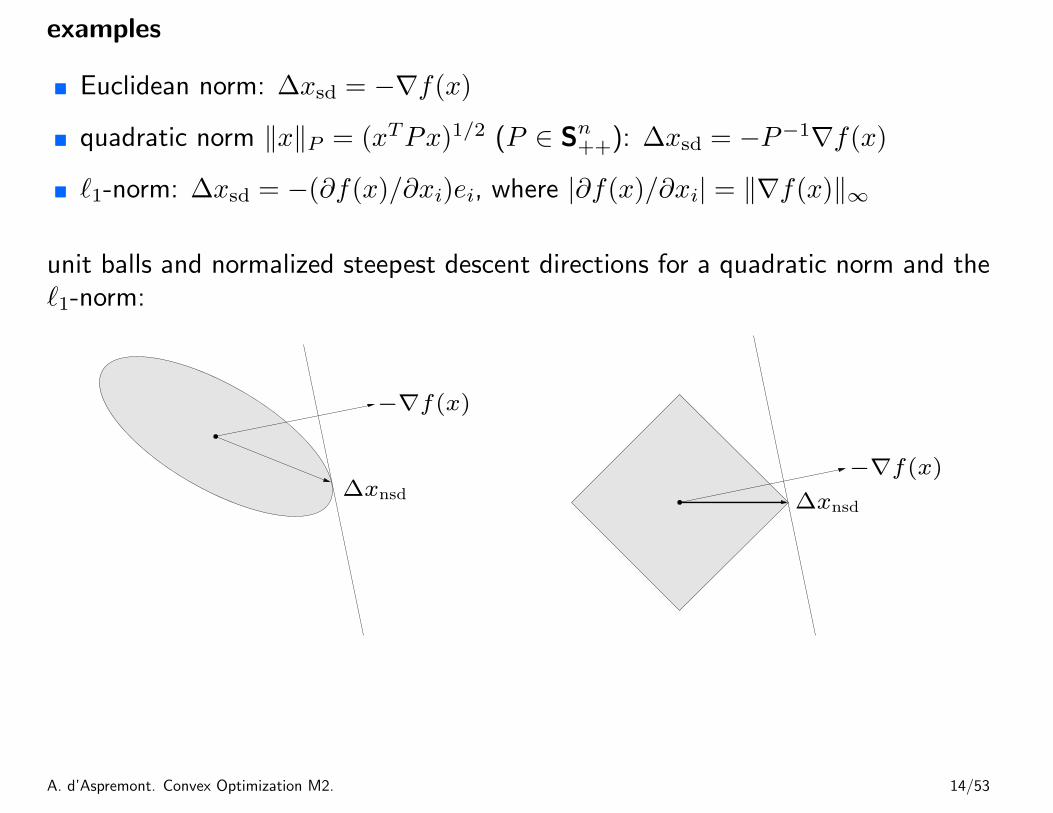
examples

� Euclidean norm: ∆xsd = −∇f(x)

� quadratic norm ‖x‖P = (xTPx)1/2 (P ∈ Sn++): ∆xsd = −P−1∇f(x)

� `1-norm: ∆xsd = −(∂f(x)/∂xi)ei, where |∂f(x)/∂xi| = ‖∇f(x)‖∞

unit balls and normalized steepest descent directions for a quadratic norm and the`1-norm:

−∇f(x)

∆xnsd

−∇f(x)

∆xnsd


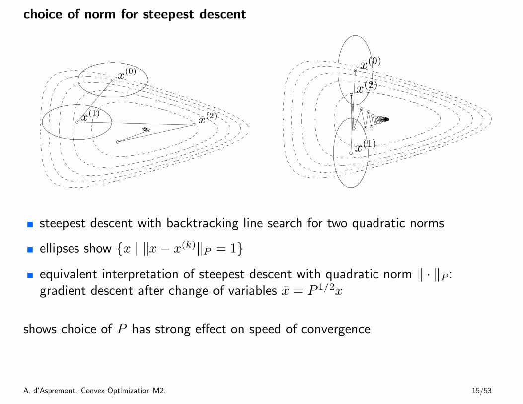
choice of norm for steepest descent

x(0)

x(1)x(2)

x(0)

x(1)

x(2)

� steepest descent with backtracking line search for two quadratic norms

� ellipses show {x | ‖x− x(k)‖P = 1}

� equivalent interpretation of steepest descent with quadratic norm ‖ · ‖P :gradient descent after change of variables x = P 1/2x

shows choice of P has strong effect on speed of convergence


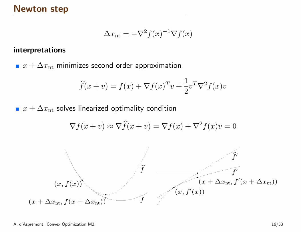
Newton step

∆xnt = −∇2f(x)−1∇f(x)

interpretations

� x+ ∆xnt minimizes second order approximation

f(x+ v) = f(x) +∇f(x)Tv +1

2vT∇2f(x)v

� x+ ∆xnt solves linearized optimality condition

∇f(x+ v) ≈ ∇f(x+ v) = ∇f(x) +∇2f(x)v = 0

f

f

(x, f(x))

(x + ∆xnt, f(x + ∆xnt))

f ′

f ′

(x, f ′(x))

(x + ∆xnt, f′(x + ∆xnt))

0


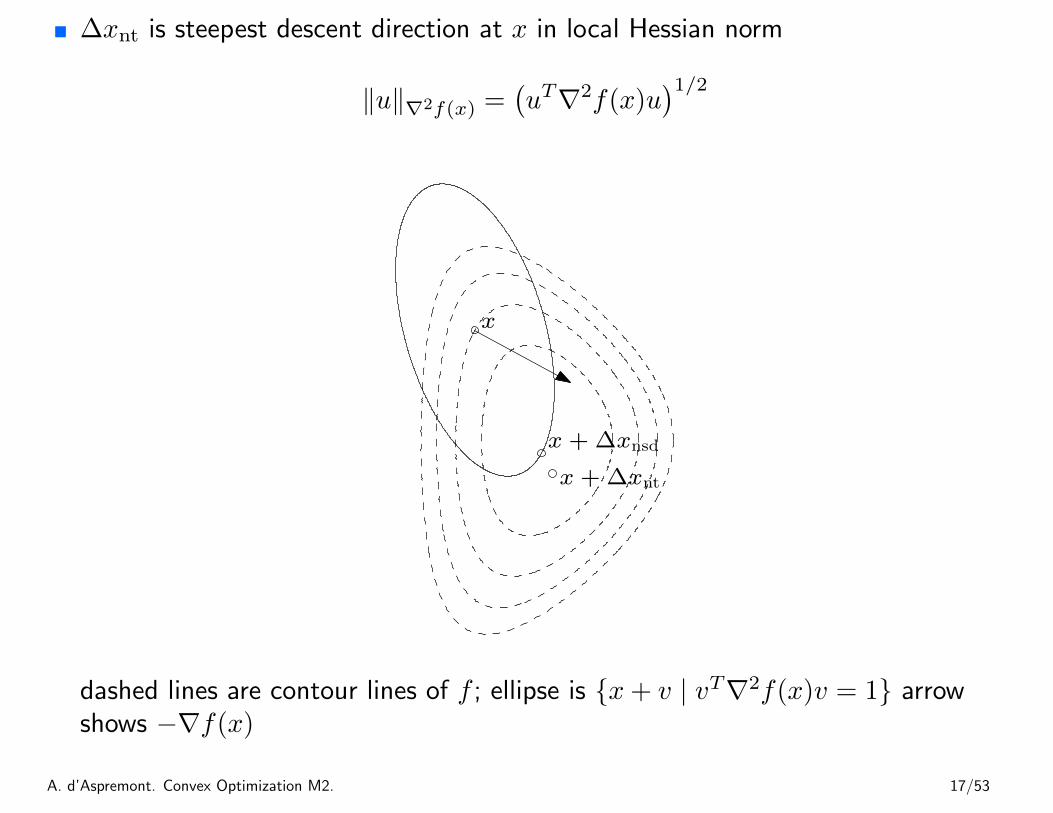
� ∆xnt is steepest descent direction at x in local Hessian norm

‖u‖∇2f(x) =(uT∇2f(x)u

)1/2

x

x + ∆xnt

x + ∆xnsd

dashed lines are contour lines of f ; ellipse is {x+ v | vT∇2f(x)v = 1} arrowshows −∇f(x)


Newton decrement

λ(x) =(∇f(x)T∇2f(x)−1∇f(x)

)1/2a measure of the proximity of x to x?

properties

� gives an estimate of f(x)− p?, using quadratic approximation f :

f(x)− infyf(y) =

1

2λ(x)2

� equal to the norm of the Newton step in the quadratic Hessian norm

λ(x) =(∆xnt∇2f(x)∆xnt

)1/2� directional derivative in the Newton direction: ∇f(x)T∆xnt = −λ(x)2

� affine invariant (unlike ‖∇f(x)‖2)


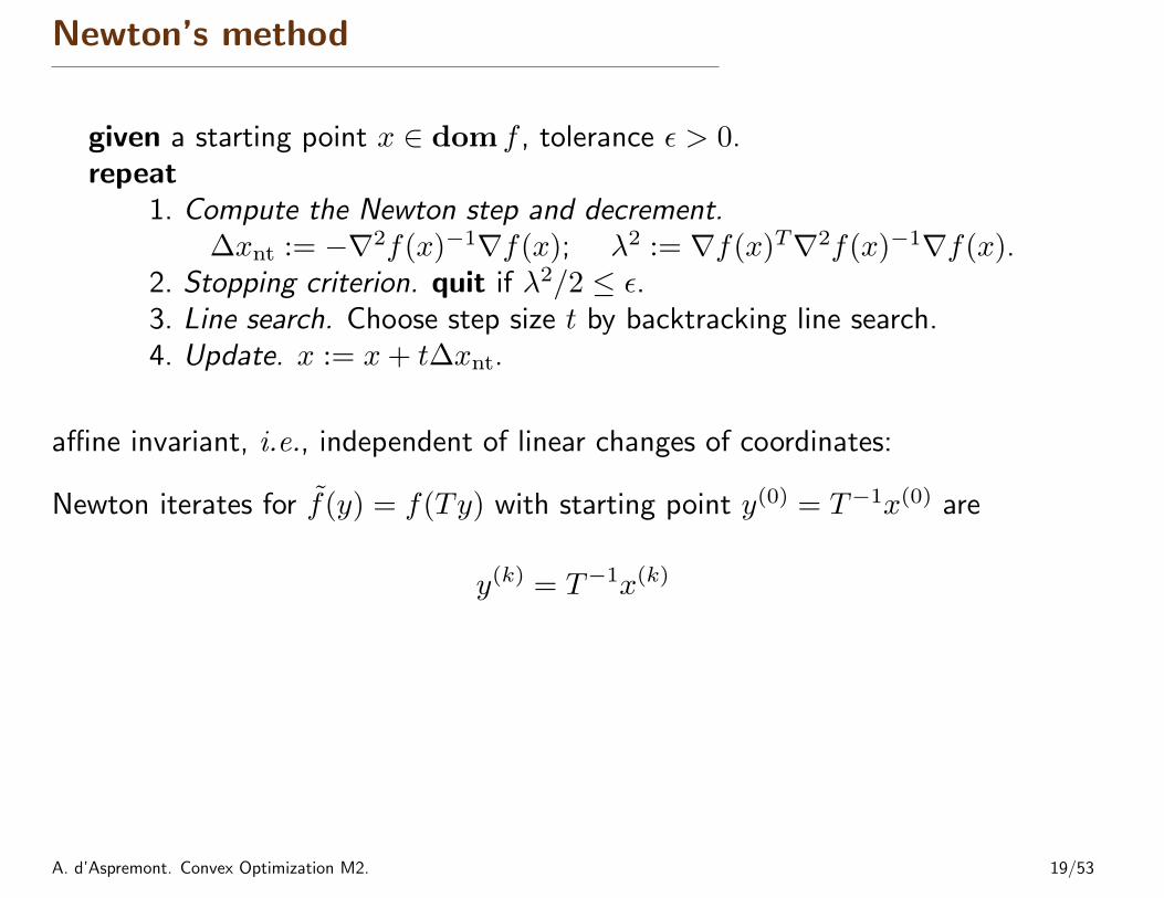
Newton’s method

given a starting point x ∈ dom f , tolerance ε > 0.repeat

1. Compute the Newton step and decrement.∆xnt := −∇2f(x)−1∇f(x); λ2 := ∇f(x)T∇2f(x)−1∇f(x).

2. Stopping criterion. quit if λ2/2 ≤ ε.3. Line search. Choose step size t by backtracking line search.4. Update. x := x+ t∆xnt.

affine invariant, i.e., independent of linear changes of coordinates:

Newton iterates for f(y) = f(Ty) with starting point y(0) = T−1x(0) are

y(k) = T−1x(k)


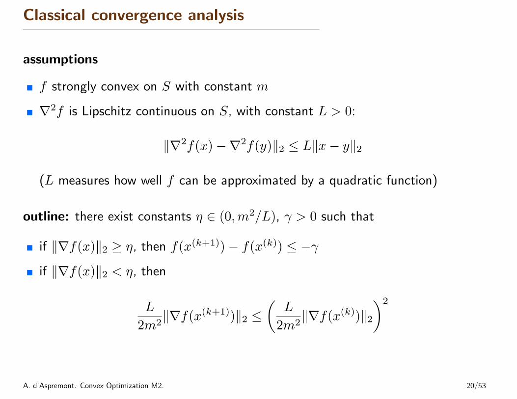
Classical convergence analysis

assumptions

� f strongly convex on S with constant m

� ∇2f is Lipschitz continuous on S, with constant L > 0:

‖∇2f(x)−∇2f(y)‖2 ≤ L‖x− y‖2

(L measures how well f can be approximated by a quadratic function)

outline: there exist constants η ∈ (0,m2/L), γ > 0 such that

� if ‖∇f(x)‖2 ≥ η, then f(x(k+1))− f(x(k)) ≤ −γ

� if ‖∇f(x)‖2 < η, then

L

2m2‖∇f(x(k+1))‖2 ≤

(L

2m2‖∇f(x(k))‖2

)2


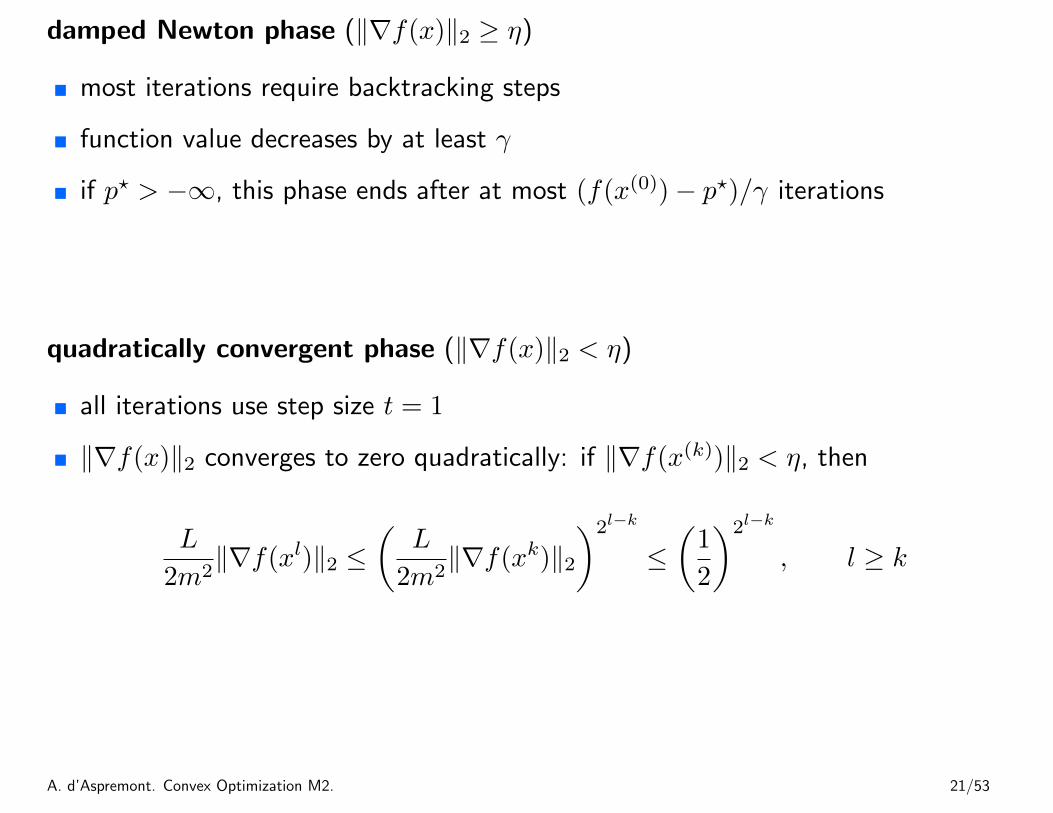
damped Newton phase (‖∇f(x)‖2 ≥ η)

� most iterations require backtracking steps

� function value decreases by at least γ

� if p? > −∞, this phase ends after at most (f(x(0))− p?)/γ iterations

quadratically convergent phase (‖∇f(x)‖2 < η)

� all iterations use step size t = 1

� ‖∇f(x)‖2 converges to zero quadratically: if ‖∇f(x(k))‖2 < η, then

L

2m2‖∇f(xl)‖2 ≤

(L

2m2‖∇f(xk)‖2

)2l−k

≤(

1

2

)2l−k

, l ≥ k


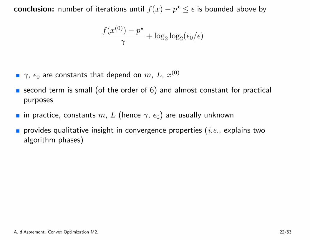
conclusion: number of iterations until f(x)− p? ≤ ε is bounded above by

f(x(0))− p?

γ+ log2 log2(ε0/ε)

� γ, ε0 are constants that depend on m, L, x(0)

� second term is small (of the order of 6) and almost constant for practicalpurposes

� in practice, constants m, L (hence γ, ε0) are usually unknown

� provides qualitative insight in convergence properties (i.e., explains twoalgorithm phases)


Examples

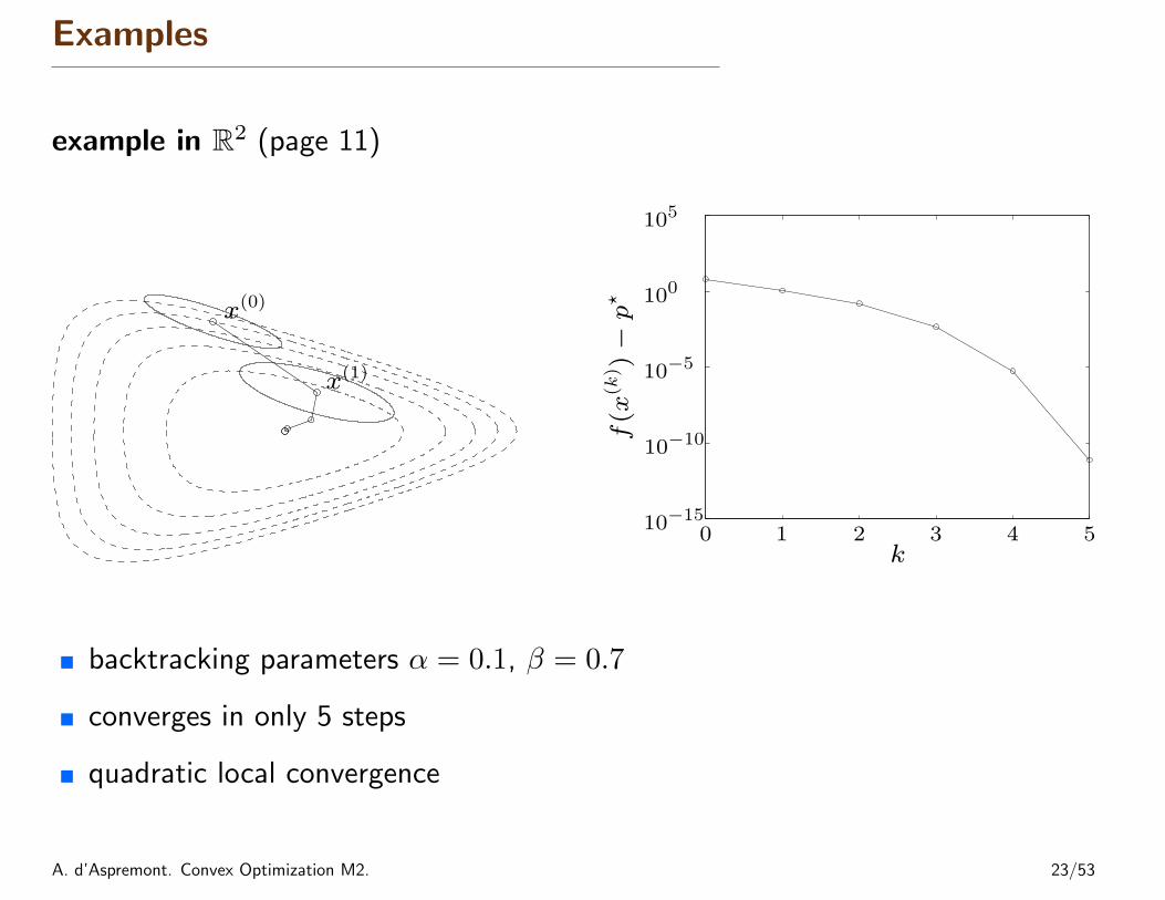
example in R2 (page 11)

x(0)

x(1)

k

f(x

(k) )

−p⋆

0 1 2 3 4 510−15

10−10

10−5

100

105

� backtracking parameters α = 0.1, β = 0.7

� converges in only 5 steps

� quadratic local convergence


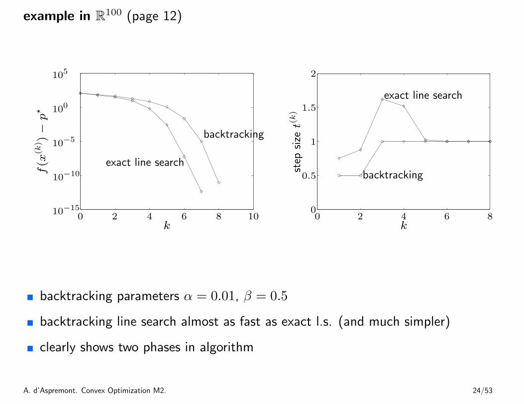
example in R100 (page 12)

k

f(x

(k) )

−p⋆

exact line search

backtracking

0 2 4 6 8 1010−15

10−10

10−5

100

105

k

step

size

t(k)

exact line search

backtracking

0 2 4 6 80

0.5

1

1.5

2

� backtracking parameters α = 0.01, β = 0.5

� backtracking line search almost as fast as exact l.s. (and much simpler)

� clearly shows two phases in algorithm


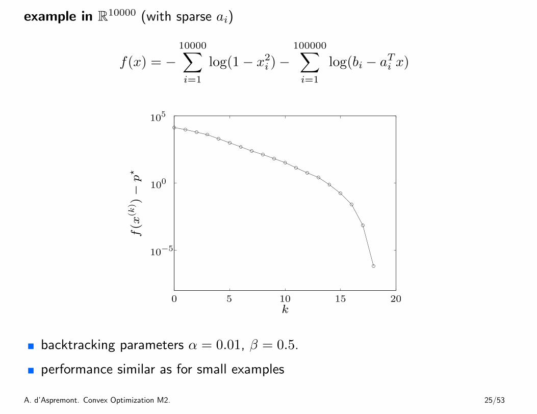
example in R10000 (with sparse ai)

f(x) = −10000∑i=1

log(1− x2i )−100000∑i=1

log(bi − aTi x)

k

f(x

(k) )

−p⋆

0 5 10 15 20

10−5

100

105

� backtracking parameters α = 0.01, β = 0.5.

� performance similar as for small examples


Self-concordance

shortcomings of classical convergence analysis

� depends on unknown constants (m, L, . . . )

� bound is not affinely invariant, although Newton’s method is

convergence analysis via self-concordance (Nesterov and Nemirovski)

� does not depend on any unknown constants

� gives affine-invariant bound

� applies to special class of convex functions (‘self-concordant’ functions)

� developed to analyze polynomial-time interior-point methods for convexoptimization


Self-concordant functions

definition

� f : R→ R is self-concordant if |f ′′′(x)| ≤ 2f ′′(x)3/2 for all x ∈ dom f

� f : Rn → R is self-concordant if g(t) = f(x+ tv) is self-concordant for allx ∈ dom f , v ∈ Rn

examples on R

� linear and quadratic functions

� negative logarithm f(x) = − log x

� negative entropy plus negative logarithm: f(x) = x log x− log x

affine invariance: if f : R→ R is s.c., then f(y) = f(ay + b) is s.c.:

f ′′′(y) = a3f ′′′(ay + b), f ′′(y) = a2f ′′(ay + b)


Self-concordant calculus

properties

� preserved under positive scaling α ≥ 1, and sum

� preserved under composition with affine function

� if g is convex with dom g = R++ and |g′′′(x)| ≤ 3g′′(x)/x then

f(x) = log(−g(x))− log x

is self-concordant

examples: properties can be used to show that the following are s.c.

� f(x) = −∑m

i=1 log(bi − aTi x) on {x | aTi x < bi, i = 1, . . . ,m}

� f(X) = − log detX on Sn++

� f(x) = − log(y2 − xTx) on {(x, y) | ‖x‖2 < y}


Convergence analysis for self-concordant functions

summary: there exist constants η ∈ (0, 1/4], γ > 0 such that

� if λ(x) > η, thenf(x(k+1))− f(x(k)) ≤ −γ

� if λ(x) ≤ η, then

2λ(x(k+1)) ≤(

2λ(x(k)))2

(η and γ only depend on backtracking parameters α, β)

complexity bound: number of Newton iterations bounded by

f(x(0))− p?

γ+ log2 log2(1/ε)

for α = 0.1, β = 0.8, ε = 10−10, bound evaluates to 375(f(x(0))− p?) + 6


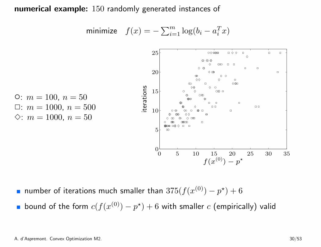
numerical example: 150 randomly generated instances of

minimize f(x) = −∑m

i=1 log(bi − aTi x)

◦: m = 100, n = 502: m = 1000, n = 5003: m = 1000, n = 50

f(x(0)) − p⋆

iterations

0 5 10 15 20 25 30 350

5

10

15

20

25

� number of iterations much smaller than 375(f(x(0))− p?) + 6

� bound of the form c(f(x(0))− p?) + 6 with smaller c (empirically) valid


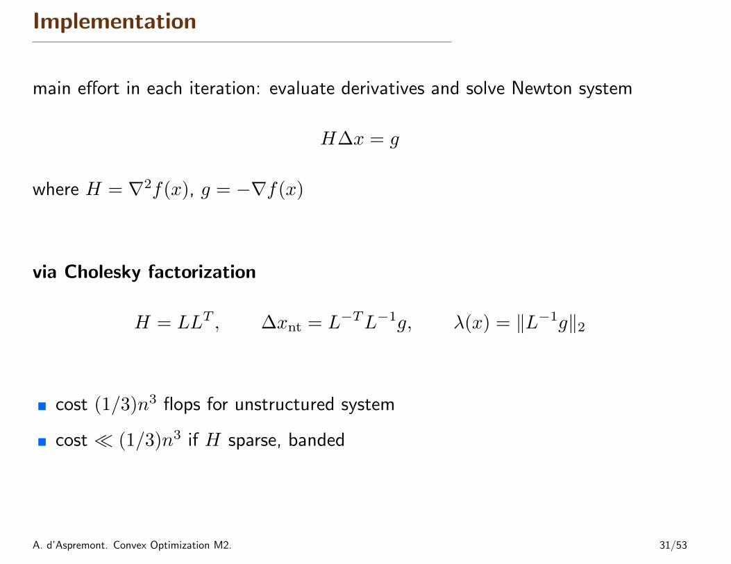
Implementation

main effort in each iteration: evaluate derivatives and solve Newton system

H∆x = g

where H = ∇2f(x), g = −∇f(x)

via Cholesky factorization

H = LLT , ∆xnt = L−TL−1g, λ(x) = ‖L−1g‖2

� cost (1/3)n3 flops for unstructured system

� cost � (1/3)n3 if H sparse, banded


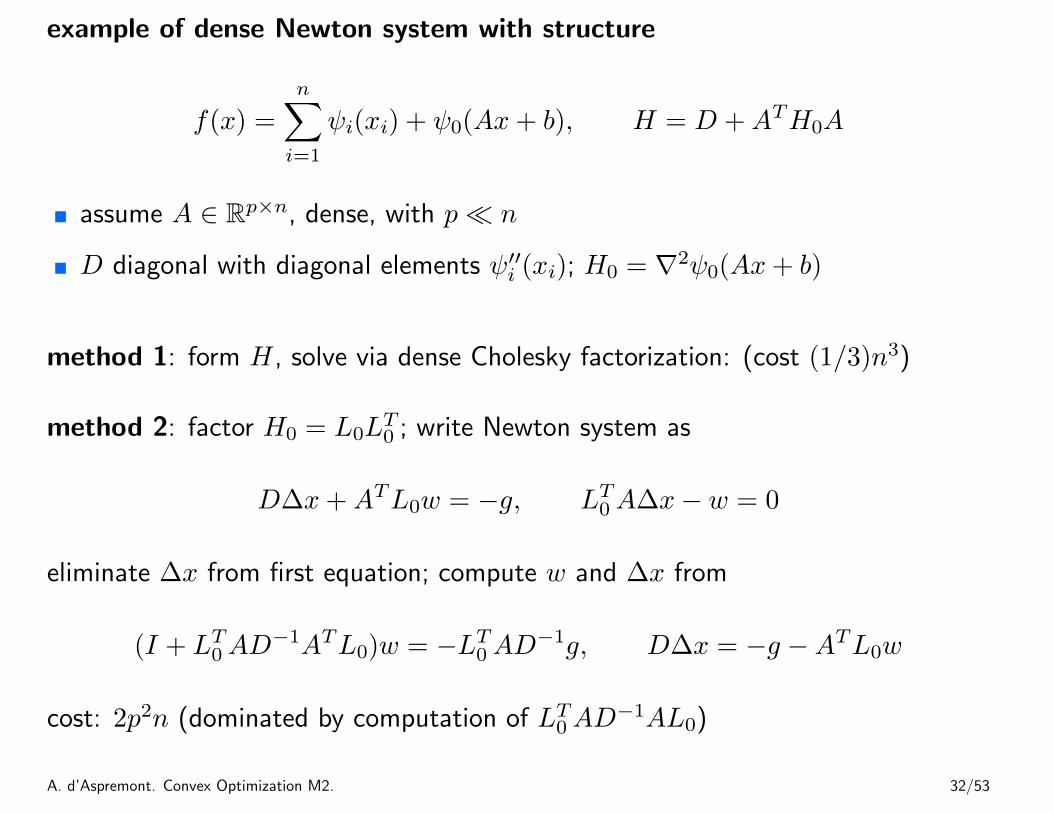
example of dense Newton system with structure

f(x) =

n∑i=1

ψi(xi) + ψ0(Ax+ b), H = D +ATH0A

� assume A ∈ Rp×n, dense, with p� n

� D diagonal with diagonal elements ψ′′i (xi); H0 = ∇2ψ0(Ax+ b)

method 1: form H, solve via dense Cholesky factorization: (cost (1/3)n3)

method 2: factor H0 = L0LT0 ; write Newton system as

D∆x+ATL0w = −g, LT0A∆x− w = 0

eliminate ∆x from first equation; compute w and ∆x from

(I + LT0AD

−1ATL0)w = −LT0AD

−1g, D∆x = −g −ATL0w

cost: 2p2n (dominated by computation of LT0AD

−1AL0)


Equality Constraints


Equality Constraints

� equality constrained minimization

� eliminating equality constraints

� Newton’s method with equality constraints

� infeasible start Newton method

� implementation


Equality constrained minimization

minimize f(x)subject to Ax = b

� f convex, twice continuously differentiable

� A ∈ Rp×n with RankA = p

� we assume p? is finite and attained

optimality conditions: x? is optimal iff there exists a ν? such that

∇f(x?) +ATν? = 0, Ax? = b


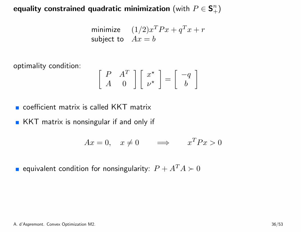
equality constrained quadratic minimization (with P ∈ Sn+)

minimize (1/2)xTPx+ qTx+ rsubject to Ax = b

optimality condition: [P AT

A 0

] [x?

ν?

]=

[−qb

]

� coefficient matrix is called KKT matrix

� KKT matrix is nonsingular if and only if

Ax = 0, x 6= 0 =⇒ xTPx > 0

� equivalent condition for nonsingularity: P +ATA � 0


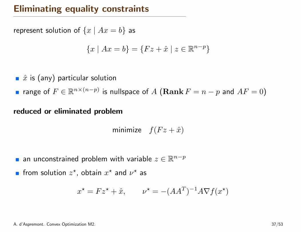
Eliminating equality constraints

represent solution of {x | Ax = b} as

{x | Ax = b} = {Fz + x | z ∈ Rn−p}

� x is (any) particular solution

� range of F ∈ Rn×(n−p) is nullspace of A (RankF = n− p and AF = 0)

reduced or eliminated problem

minimize f(Fz + x)

� an unconstrained problem with variable z ∈ Rn−p

� from solution z?, obtain x? and ν? as

x? = Fz? + x, ν? = −(AAT )−1A∇f(x?)


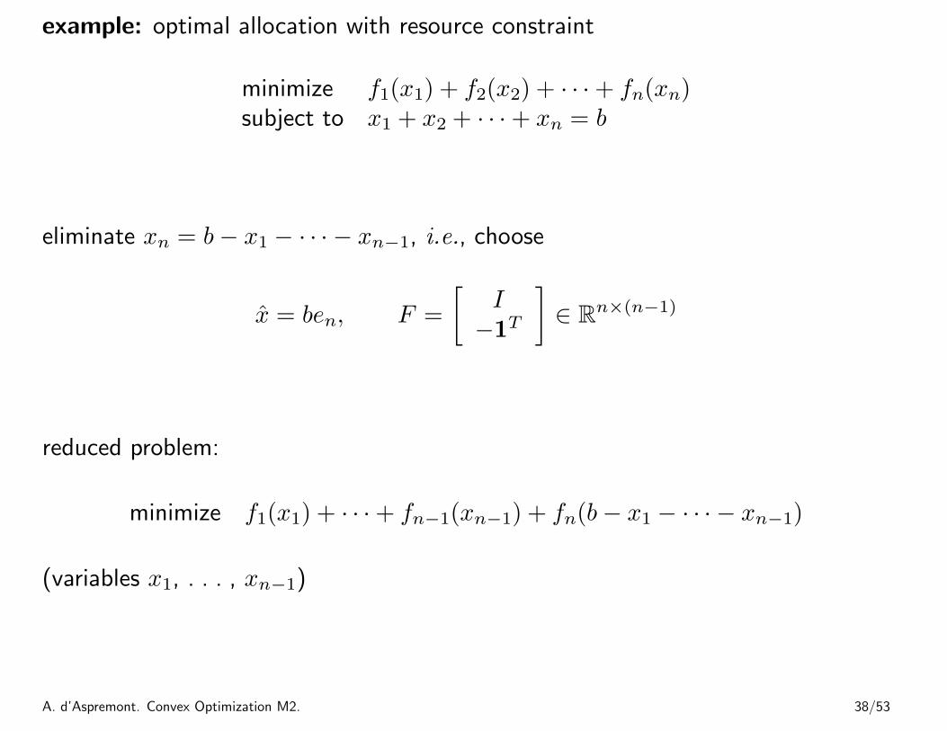
example: optimal allocation with resource constraint

minimize f1(x1) + f2(x2) + · · ·+ fn(xn)subject to x1 + x2 + · · ·+ xn = b

eliminate xn = b− x1 − · · · − xn−1, i.e., choose

x = ben, F =

[I−1T

]∈ Rn×(n−1)

reduced problem:

minimize f1(x1) + · · ·+ fn−1(xn−1) + fn(b− x1 − · · · − xn−1)

(variables x1, . . . , xn−1)


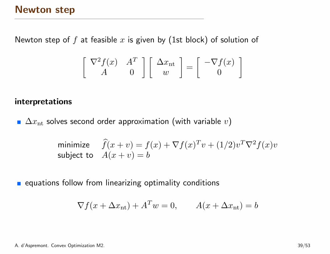
Newton step

Newton step of f at feasible x is given by (1st block) of solution of[∇2f(x) AT

A 0

] [∆xntw

]=

[−∇f(x)

0

]

interpretations

� ∆xnt solves second order approximation (with variable v)

minimize f(x+ v) = f(x) +∇f(x)Tv + (1/2)vT∇2f(x)vsubject to A(x+ v) = b

� equations follow from linearizing optimality conditions

∇f(x+ ∆xnt) +ATw = 0, A(x+ ∆xnt) = b


Newton decrement

λ(x) =(∆xTnt∇2f(x)∆xnt

)1/2=(−∇f(x)T∆xnt

)1/2properties

� gives an estimate of f(x)− p? using quadratic approximation f :

f(x)− infAy=b

f(y) =1

2λ(x)2

� directional derivative in Newton direction:

d

dtf(x+ t∆xnt)

∣∣∣∣t=0

= −λ(x)2

� in general, λ(x) 6=(∇f(x)T∇2f(x)−1∇f(x)

)1/2


Newton’s method with equality constraints

given starting point x ∈ dom f with Ax = b, tolerance ε > 0.

repeat1. Compute the Newton step and decrement ∆xnt, λ(x).2. Stopping criterion. quit if λ2/2 ≤ ε.3. Line search. Choose step size t by backtracking line search.4. Update. x := x+ t∆xnt.

� a feasible descent method: x(k) feasible and f(x(k+1)) < f(x(k))

� affine invariant


Newton’s method and elimination

Newton’s method for reduced problem

minimize f(z) = f(Fz + x)

� variables z ∈ Rn−p

� x satisfies Ax = b; RankF = n− p and AF = 0

� Newton’s method for f , started at z(0), generates iterates z(k)

Newton’s method with equality constraints

when started at x(0) = Fz(0) + x, iterates are

x(k+1) = Fz(k) + x

hence, don’t need separate convergence analysis


Newton step at infeasible points

2nd interpretation of page 39 extends to infeasible x (i.e., Ax 6= b)

linearizing optimality conditions at infeasible x (with x ∈ dom f) gives[∇2f(x) AT

A 0

] [∆xntw

]= −

[∇f(x)Ax− b

](1)

primal-dual interpretation

� write optimality condition as r(y) = 0, where

y = (x, ν), r(y) = (∇f(x) +ATν,Ax− b)

� linearizing r(y) = 0 gives r(y + ∆y) ≈ r(y) +Dr(y)∆y = 0:[∇2f(x) AT

A 0

] [∆xnt∆νnt

]= −

[∇f(x) +ATν

Ax− b

]same as (1) with w = ν + ∆νnt


Infeasible start Newton method

given starting point x ∈ dom f , ν, tolerance ε > 0, α ∈ (0, 1/2), β ∈ (0, 1).

repeat1. Compute primal and dual Newton steps ∆xnt, ∆νnt.2. Backtracking line search on ‖r‖2.

t := 1.while ‖r(x+ t∆xnt, ν + t∆νnt)‖2 > (1− αt)‖r(x, ν)‖2, t := βt.

3. Update. x := x+ t∆xnt, ν := ν + t∆νnt.until Ax = b and ‖r(x, ν)‖2 ≤ ε.

� not a descent method: f(x(k+1)) > f(x(k)) is possible

� directional derivative of ‖r(y)‖22 in direction ∆y = (∆xnt,∆νnt) is

d

dt‖r(y + ∆y)‖2

∣∣∣∣t=0

= −‖r(y)‖2


Solving KKT systems

[H AT

A 0

] [vw

]= −

[gh

]solution methods

� LDLT factorization

� elimination (if H nonsingular)

AH−1ATw = h−AH−1g, Hv = −(g +ATw)

� elimination with singular H: write as[H +ATQA AT

A 0

] [vw

]= −

[g +ATQh

h

]

with Q � 0 for which H +ATQA � 0, and apply elimination


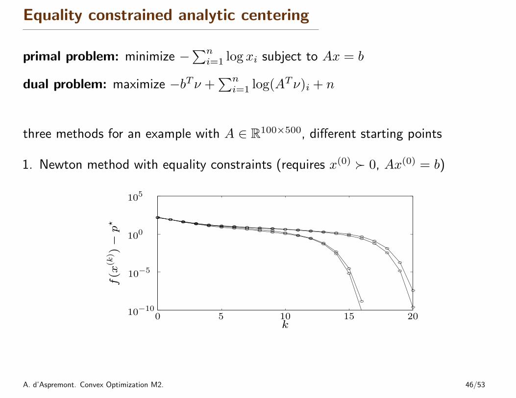
Equality constrained analytic centering

primal problem: minimize −∑n

i=1 log xi subject to Ax = b

dual problem: maximize −bTν +∑n

i=1 log(ATν)i + n

three methods for an example with A ∈ R100×500, different starting points

1. Newton method with equality constraints (requires x(0) � 0, Ax(0) = b)

k

f(x

(k) )

−p⋆

0 5 10 15 2010−10

10−5

100

105


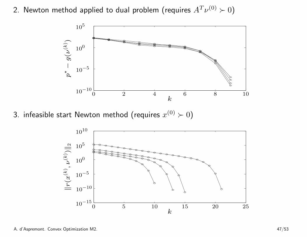
2. Newton method applied to dual problem (requires ATν(0) � 0)

k

p⋆−

g(ν

(k) )

0 2 4 6 8 1010−10

10−5

100

105

3. infeasible start Newton method (requires x(0) � 0)

k

‖r(x

(k) ,ν(k

) )‖2

0 5 10 15 20 2510−15

10−10

10−5

100

105

1010


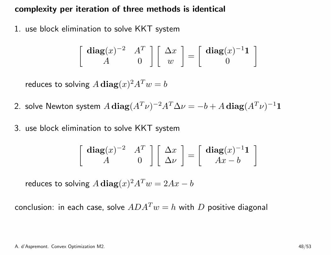
complexity per iteration of three methods is identical

1. use block elimination to solve KKT system[diag(x)−2 AT

A 0

] [∆xw

]=

[diag(x)−11

0

]

reduces to solving Adiag(x)2ATw = b

2. solve Newton system Adiag(ATν)−2AT∆ν = −b+Adiag(ATν)−11

3. use block elimination to solve KKT system[diag(x)−2 AT

A 0

] [∆x∆ν

]=

[diag(x)−11Ax− b

]

reduces to solving Adiag(x)2ATw = 2Ax− b

conclusion: in each case, solve ADATw = h with D positive diagonal


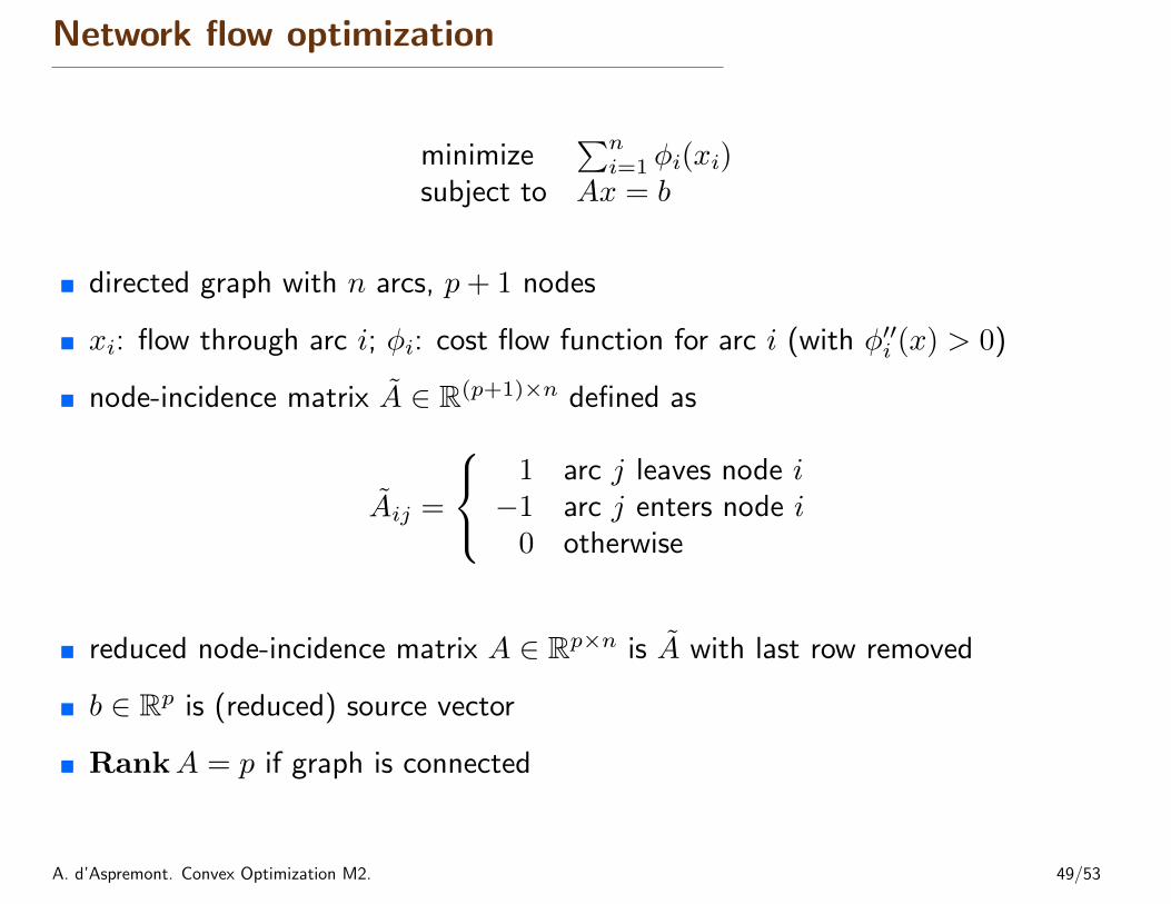
Network flow optimization

minimize∑n

i=1 φi(xi)subject to Ax = b

� directed graph with n arcs, p+ 1 nodes

� xi: flow through arc i; φi: cost flow function for arc i (with φ′′i (x) > 0)

� node-incidence matrix A ∈ R(p+1)×n defined as

Aij =

1 arc j leaves node i−1 arc j enters node i

0 otherwise

� reduced node-incidence matrix A ∈ Rp×n is A with last row removed

� b ∈ Rp is (reduced) source vector

� RankA = p if graph is connected


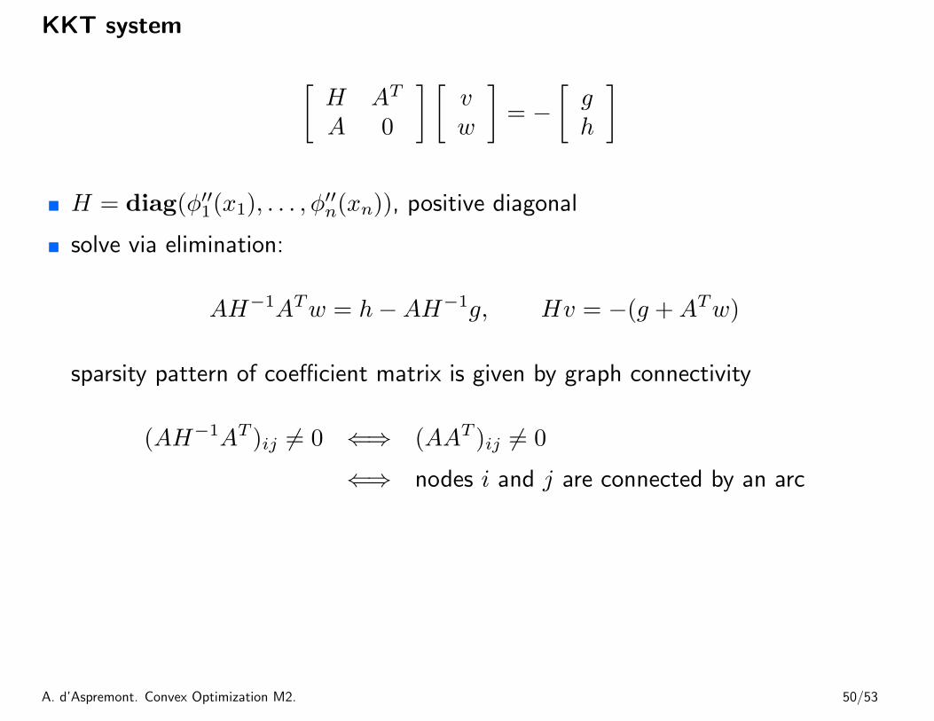
KKT system

[H AT

A 0

] [vw

]= −

[gh

]

� H = diag(φ′′1(x1), . . . , φ′′n(xn)), positive diagonal

� solve via elimination:

AH−1ATw = h−AH−1g, Hv = −(g +ATw)

sparsity pattern of coefficient matrix is given by graph connectivity

(AH−1AT )ij 6= 0 ⇐⇒ (AAT )ij 6= 0

⇐⇒ nodes i and j are connected by an arc


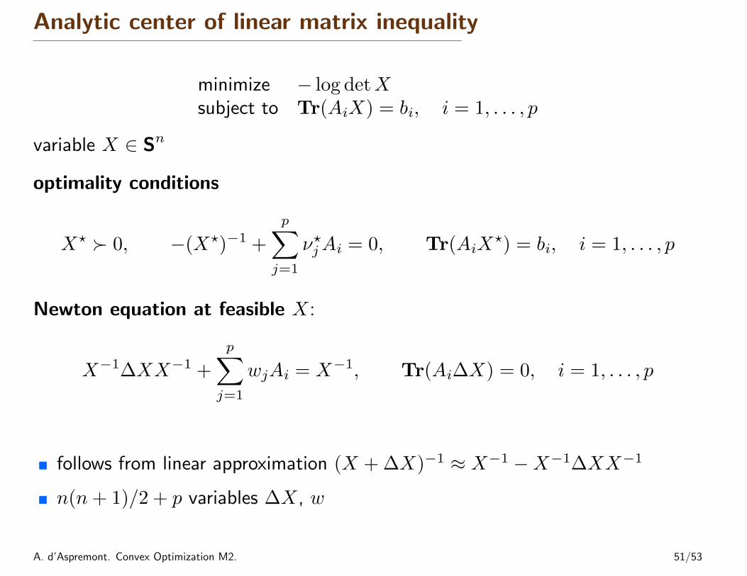
Analytic center of linear matrix inequality

minimize − log detXsubject to Tr(AiX) = bi, i = 1, . . . , p

variable X ∈ Sn

optimality conditions

X? � 0, −(X?)−1 +

p∑j=1

ν?jAi = 0, Tr(AiX?) = bi, i = 1, . . . , p

Newton equation at feasible X:

X−1∆XX−1 +

p∑j=1

wjAi = X−1, Tr(Ai∆X) = 0, i = 1, . . . , p

� follows from linear approximation (X + ∆X)−1 ≈ X−1 −X−1∆XX−1

� n(n+ 1)/2 + p variables ∆X, w


solution by block elimination

� eliminate ∆X from first equation: ∆X = X −∑p

j=1wjXAjX

� substitute ∆X in second equation

p∑j=1

Tr(AiXAjX)wj = bi, i = 1, . . . , p (2)

a dense positive definite set of linear equations with variable w ∈ Rp

flop count (dominant terms) using Cholesky factorization X = LLT :

� form p products LTAjL: (3/2)pn3

� form p(p+ 1)/2 inner products Tr((LTAiL)(LTAjL)): (1/2)p2n2

� solve (2) via Cholesky factorization: (1/3)p3


Documents

Convex Optimization M2 - École Normale Supérieureaspremon/PDF/MVA/UnconstrainedEquality.pdfConvex Optimization M2. 5/53. Strong convexity and implications fis strongly convex on