Convexity and Optimization

Statistical Machine Learning, Spring 2015

Ryan Tibshirani (with Larry Wasserman)

1 An entirely too brief motivation

1.1 Why optimization?

• Optimization problems are ubiquitous in statistics and machine learning. A huge number ofproblems that we consider in these disciplines (and, other disciplines) can indeed be posed asoptimization tasks

• But why bother studying the details? Other people have already understood the importanceof optimization and have provided us with fast software for various optimization algorithms

• Two major reasons: (1) different algorithms can perform (sometimes drastically) better orworse in different scenarios, and an understanding of why this happens requires an under-standing of optimization; (2) often times, understanding a problem from the optimizationperspective can contribute to our statistical understanding of the problem as well

• Since this is a theoretical course, we will ignore reason (1), and focus on reason (2)

1.2 Why convexity?

• Simply: because we can broadly understand and solve convex optimization problems. Non-convex ones are understood and solved more on a case by case basis (this isn’t entirely true)

• Historically, linear programs were the focus in the optimization community, and initially, itwas thought that the major divide was between linear and nonlinear optimization problems;later people discovered that some nonlinear problems were much harder than others, and the“right” divide was between convex and nonconvex problems

1.3 Two great references

• There are many great books on convexity and optimization. They can be roughly divided intobooks focused on convex analysis (the turf of mathematicians) and books focused on convexoptimization (the turf of engineers). Here are two such books:

– Boyd & Vandenberghe (2004)

– Rockafellar (1970)

Our presentation here is based on these two excellent books, especially Boyd & Vandenberghe(2004). Combined, the two provide a pretty complete coverage

1.4 A shameless plug

• You should take our Convex Optimization course (10-725/36-725), you’ll learn a lot more

1

2 Convex sets

2.1 Basic definitions

• A set C ⊆ Rn is convex provided that, for any x, y ∈ C and θ ∈ [0, 1], we have

θx+ (1− θ)y ∈ C,

i.e., the line segment joining x, y lies entirely in C

• In a more general probabilistic form: if X ∈ Rn is a random variable supported on a convexset C ⊆ Rn, then E(X) ∈ C

• A convex combination of points x1, . . . xk ∈ Rn is a combination of the form

θ1x1 + θ2x2 + . . .+ θkxk,

where θi ≥ 0, i = 1, . . . k and∑ki=1 θi = 1

• The convex hull of a set C is the set of all convex combinations of points in C,

conv(C) ={θ1x1 + θ2x2 + . . .+ θkxk : xi ∈ C, θi ≥ 0 for i = 1, . . . k, and

k∑i=1

θi = 1}

• If you’ve forgotten, you should remind yourself of the basics of point-set topology: open andclosed sets, closure of a set (written cl(S)), and interior and boundary of a set (written int(S)and bd(S))

2.2 Some examples

• The empty set ∅ is convex

• Lines, rays, line segments, linear spaces, and affine spaces are all convex

• A hyperplane is convex: this is a set of the form {x : aTx = b}

• A halfspace is convex: this is a set of the form {x : aTx ≤ b}

• A norm ball is convex: given a norm ‖ · ‖ on Rn (e.g., the `p norm, ‖ · ‖p, for p ≥ 1) this hasthe form {x : ‖x‖ ≤ t}

• A polyhedron is convex: this is the intersection of some finite number of halfspaces, as in

{x : aTi x ≤ bi, i = 1, . . .m}.

We can abbreviate this as {x : Ax ≤ b}, where b = (b1, . . . bm) ∈ Rm, A ∈ Rm×n with rows ai,i = 1, . . .m, and the inequality Ax ≤ b is interpreted componentwise

• Note: we can also write a polyhedron as {x : Ax ≤ b, Cx = d}. (Why?)

• Any bounded polyhedron (called a polytope) can also be written as the convex hull of a finiteset of points; this is called its V-representation. The original representation given above, asan intersection of halfspaces, is called its H-representation

• Simplexes are a special case of polyhedra that are given by taking the convex hull of a set ofpoints {x0, . . . xk} ⊆ Rn that are affinely independent, which means that x1 − x0, . . . xk − x0

are linearly independent. In particular, this is a k-dimensional simplex in Rn

2

• The canonical simplex is the probability simplex, given by the convex hull of {e1, . . . en} ⊆ Rn,the standard basis vectors in Rn, which can be written as

{θ : θ ≥ 0, 1T θ = 1}.

Note again that the inequality θ ≥ 0 is to be interpreted componentwise (and we will, withoutdistinction, use 1 to denote the vector of 1s whenever convenient)

• Consider the set of symmetric n× n matrices,

Sn = {X ∈ Rn×n : X = XT }.

Think of this as a vector space of dimension n(n+1)/2. Now consider the subset of this vectorspace

Sn+ = {X ∈ Sn : X � 0},where X � 0 means that X is positive semidefinite. We call Sn+ the positive semidefinite cone,and it is a convex set (again, think of it as a set in the ambient n(n + 1)/2 vector space ofsymmetric matrices)

2.3 Key properties

• Separating hyperplane theorem: if C,D are nonempty, and disjoint (C ∩D = ∅) convex sets,then there exists a 6= 0 and b such that C ⊆ {x : aTx ≤ b} and D ⊆ {x : aTx ≥ b}

• Supporting hyperplane theorem: if C is a nonempty convex set, and x0 ∈ bd(C), then thereexists a supporting hyperplane to C at x0, i.e., there exists a 6= 0 and b such that aTx0 = band C ⊆ {x : aTx ≤ b}

• Closed halfspace representation: if C is a closed convex set, then it can be represented as theintersection of all halfspaces that contain it,

C =⋂ {

H : H is a halfspace, and H ⊇ C}

2.4 Operations that preserve convexity

• Convexity of all sets in Section 2.2 can be verified directly from the definition. Often though,to check that a set S is convex, it is easier to start with a set of basic sets that we know areconvex (such as those in Section 2.2), and recognize that our set S of interest is given by atransformation of one of these basic sets, via an operation that preserves convexity

• The intersection of any number of convex sets is convex. This even holds for an (uncountably)infinite number of sets

E.g., from this we can show that the positive semidefinite cone Sn+ is convex, because

Sn+ ={X ∈ Sn : aTXa ≥ 0 for all a ∈ Rn

}=⋂a∈Rn

{X ∈ Sn : aTXa ≥ 0}.

Note that, for a fixed a ∈ Rn, the term aTXa =∑ni,j=1 aiajXij is actually a linear function

in X, so the above is an intersection of halfspaces in X, and therefore convex

3

• Affine images and affine preimages of convex sets are convex. I.e., if f : Rn → Rm is an affinefunction, meaning that f(x) = Ax+ b, and S ⊆ Rn, T ⊆ Rm are convex, then both

f(S) = {f(x) : x ∈ S}

andf−1(T ) = {x : f(x) ∈ T}

are convex

E.g., from this we can show that the solution set of a linear matrix inequality{x ∈ Rk : x1A1 + x2A2 + . . .+ xkAk � B

},

where A1, . . . Ak, B ∈ Sn is convex. To see this, note that this set is the inverse image of Sn+under the affine function f : Rk → Sn,

f(x) = B − (x1A1 + x2A2 + . . .+ xkAk)

• Note in particular that both scaling and translation preserve convexity (special cases of affineimages), i.e., if S ⊆ Rn is convex then

αS = {αx : x ∈ S}

is convex for any α ∈ R, andS + c = {x+ c : x ∈ S}

is convex for any c ∈ Rn

• Perspective images and perpsective preimages of convex sets are also convex. The perspectivefunction P ∈ Rn+1, with domain dom(P ) = Rn × R++ (here R++ denotes the set of positivereals), is defined as

P (x, t) = x/t = (x1/t, . . . xn/t).

Then for any convex S ⊆ dom(P ) ⊆ Rn+1, the image

P (S) = {P (z) : z ∈ S}

is convex, and for any convex T ⊆ Rn, the preimage

P−1(T ) = {(x, t) : t > 0, x/t ∈ T}

is also convex

• Linear-fractional images and linear-fractional preimages are convex. A linear-fractional func-tion is the perspective function composed with an affine function, i.e., if g : Rn × Rm+1 isaffine,

g(x) =

[AcT

]x+

[bd

],

and P : Rm+1 → Rm is the perspective map, then f = P ◦ g : Rn → Rm is a linear-fractionalfunction. Note

f(x) =Ax+ b

cTx+ d,

with domain dom(f) = {x : cTx+ d > 0}. From what we know already, if S ⊆ dom(f) ⊆ Rnis convex, then the image f(S) = P (g(S)) is convex, and also, if T ⊆ Rm+1 is convex, the thepreimage f−1(T ) = g−1(P−1(T )) is convex

4

E.g., using this we can show the following fact. Let U, V be random variables taking discretevalues in {1, . . . n} and {1, . . .m}, respectively, and let S ⊆ Rnm be a set of joint probabilitiesfor U, V . In other words, each p ∈ C defines a probability distribution over U, V , as inpij = P(U = i, V = j). If S is convex, then the set of conditional probabilities of U given V isalso convex.

Why? The set of conditional probabilities of U given V is{q ∈ Rnm : qij =

pij∑nk=1 pkj

, for some p ∈ C}.

This is the image of C under a linear-fractional function, and is hence convex provided thatC is convex

3 Convex functions

3.1 Basic definitions

• In a rough sense, convex functions are even more important than convex sets, because we usethem more (though this sounds funny, because the two are intimately related)

• A function f : Rn → R is convex if its domain dom(f) is convex, and for any x, y ∈ dom(f)and θ ∈ [0, 1],

f(θx+ (1− θ)y

)≤ θf(x) + (1− θ)f(y).

In words, the function lies below the line segment joining its evaluations at x, y. A function isstrictly convex if this same inequality holds strictly for x 6= y and θ ∈ (0, 1),

f(θx+ (1− θ)y

)< θf(x) + (1− θ)f(y)

• A function f is concave or strictly concave if −f is convex or strictly convex, respectively

• Affine functions, i.e., such that f(x) = aTx+ b, are both convex and concave (conversely, anyfunction that is both convex and concave is affine)

• A function f is strongly convex with parameter m > 0 (written m-strongly convex) providedthat

f(x)− m

2‖x‖22

is a convex function. In rough terms, this means that f is “as least as convex” as a quadraticfunction. This is the strongest form of convexity (hence its name), so that strong convexityimplies strict convexity implies convexity

3.2 Some examples

• Examples on R: the exponential function eax is convex for any a ∈ R; the power function xa

is convex on R++ for any a ≥ 1 or a ≤ 0; the negative entropy function x log x is convex onR++; the log function log x is concave on R++; the power function xa is concave on R++ forany 0 ≤ a ≤ 1; the affine function ax+ b is both convex and concave

• Norms are convex, i.e., f : Rn → R defined by f(x) = ‖x‖ is a convex function, for any norm‖ · ‖

5

• An important special case is the `p norm, ‖ · ‖p, for p ≥ 1. Recall that this is defined as

‖x‖p =( n∑i=1

|xi|p)1/p

when p <∞, and‖x‖∞ = max

i=1,...n|xi|.

• Two other important special cases are the operator (spectral) and trace (nuclear) norms formatrices. Recall that if X ∈ Rm×n has singular values σ1(X) ≥ σ2(X) ≥ . . . ≥ σr(X) ≥ 0,where r = rank(X) ≤ min{m,n}, then its operator (or spectral) norm is

‖X‖op = σ1(X),

and its trace (or nuclear) norm is

‖X‖tr =r∑i=1

σr(X)

• The indicator function f(x) = IC(x) of a convex set C ⊆ Rn is convex. This is defined as

IC(x) =

{0 x ∈ C∞ x /∈ C

• The quadratic function f(x) = 12x

TQx+ cTx+ b is convex provided that Q � 0

• The least squares criterion f(x) = ‖Ax− b‖22 = xTATAx− 2bTAx+ bT b is hence convex

• The max function f(x) = max{x1, . . . xn} is convex

• The function f(x) = log(∑ni=1 exp(xi)) is convex, and called the log-sum-exp function. This is

often viewed as an (infinitely differentiable) approximation to the max function, since

max{x1, . . . xn} ≤ f(x) ≤ max{x1, . . . xn}+ log n

3.3 Key properties

• A convex function is continuous on the relative interior of its domain; it can only have pointsof discontinuity on its relative boundary

• A function is convex if and only its restriction to any line is convex. That is, f : Rn → R isconvex if and only if g(t) = f(x+ tv) is convex in t ∈ R (on its domain {t : x+ tv ∈ dom(f)}),for all v ∈ Rn

E.g., from this we can show that the function f : Sn → R, f(X) = log detX, with dom(f) =Sn++ = {X ∈ Sn : X � 0}, is concave

• First-order characterization: suppose that f is differentiable (and write ∇f for its gradient).Then f is convex if and only if dom(f) is convex, and for all x, y ∈ dom(f),

f(y) ≥ f(x) +∇f(x)T (y − x).

In words, the function always dominates its first order (linear) Taylor approximation. It’s ananalogous story for strict convexity: the condition is that for all x 6= y,

f(y) > f(x) +∇f(x)T (y − x)

6

E.g., from the first-order characterization, we can deduce a useful property: if ∇f(x) = 0 for aconvex function f , then f(y) ≥ f(x) for all y, so x is a minimizer of f . Further, if f is strictlyconvex, then x is the unique minimizer

• Second-order characterization: suppose that f is twice differentiable (and we write ∇2f for itsHessian). Then f is convex if and only if dom(f) is convex, and

∇2f(x) � 0

for all x ∈ dom(f). Note that ∇2f(x) � 0 for all x ∈ dom(f) implies strict convexity—butthe converse is not true!

E.g., using this second-order characterization, we can verify the convexity of the quadraticfunction f(x) = xTQx+ cTx+ b when Q � 0 (and strict convexity when Q � 0). We can alsoverify that f : Rn → R defined by

f(x) = log( n∑i=1

exp(xi))

is convex

• Strong convexity characterizations: if f is differentiable, then m-strong convexity is equivalentto dom(f) being convex and

f(y) ≥ f(x) +∇f(x)T (y − x) +m

2‖y − x‖22

for all x, y ∈ dom(f). I.e., f is lower bounded by its second order (quadratic) approximation,rather then only its first order (linear) approximation, which is implied by regular convexity

If f is twice differentiable, then m-strong convexity is equivalent to dom(f) being convex and

∇2f(x) � mI

for all x ∈ dom(f), i.e., the smallest eigenvalue of the Hessian is lower bounded by m, every-where

• A convex function f has convex level sets,

{x ∈ dom(f) : f(x) ≤ t},

for any t ∈ R. The converse is not true

• Epigraph characterization: a function f is convex if and only if its epigraph

{(x, t) ∈ dom(f)× R : f(x) ≤ t}

is a convex set. This ties together convexity for functions and sets; in fact many properties ofconvex functions can be proven from those for convex sets

• Jensen’s inequality: if f is convex, and X is a random variable supported on dom(f), then

f(E(X)

)≤ E

(f(X)

).

This is a more general probabilistic form of the basic inequality for convexity

7

3.4 Operations that preserve convexity

• As was true for convex sets, the easiest way to prove convexity of a function is often to showthat it can be built up from simple convex functions, using operations that preserve convexity

• Nonnegative linear combinations: if f1, . . . fm are convex, then

a1f1 + . . .+ amfm

is convex for any a1, . . . am ≥ 0

• Affine composition: if f is convex, then g(x) = f(Ax+ b) is convex

• Pointwise maximum: if f1, . . . fm are convex, then

f(x) = max{f1(x), . . . fm(x)}

are convex. This extends to (uncountably) infinitely many functions: if fs(x) is convex for anys ∈ S, then

f(x) = maxs∈S

fs(x)

is convex

We can use this to show some fairly nonobvious functions are convex. E.g., the maximumdistance to an arbitrary set C ⊆ Rn,

f(x) = maxy∈C

‖x− y‖,

in any norm ‖ · ‖, is convex. This is because ‖x− y‖ is convex in x for any fixed y. Also, theoptimal weighted least squares cost,

f(w) = minβ∈Rp

n∑i=1

wi(yi − xTi β)2,

is concave as a function of the weights w ∈ Rn, with domain

dom(f) ={w : min

β∈Rp

n∑i=1

wi(yi − xTi β)2 > −∞}.

This is because each∑ni=1 wi(yi − xTi β)2, for fixed β, is affine and hence concave in w, so the

pointwise minimum f is also concave

• Partial minimization: if f(x, y) is convex in x, y, and C is a convex and nonempty set, then

g(x) = miny∈C

f(x, y)

is convex in x, provided that g(x) > −∞ for all x in its domain,

dom(g) = {x : (x, y) ∈ dom(f) for some y ∈ C}

Again, we can use this to show some fairly nonobvious properties. E.g., the minimum distanceto a convex set C,

f(x) = miny∈C‖x− y‖,

8

in any norm ‖ · ‖, is convex. This is because ‖x − y‖ is convex in x, y, and we have assumedthat C is convex. (N.B. the maximum distance to any set is a convex function.) Also, supposethat [

A BBT C

]� 0

and sof(x, y) = xTAx+ 2xTBy + yTCy

is convex is x, y. Then we know that

g(x) = miny∈Rn

f(x, y)

is convex in x; a simple calculation shows that, assuming C is invertible,

g(x) = xT (A−BC−1BT )x.

Therefore, for g to be convex, we know that the Schur complement has to be positive semidef-inite,

A−BC−1BT � 0

• Composition: this is a bit tricky, as composition rules that preserve convexity (or concavity)rely on monotonicity conditions. Here are a few results to remember, in the setting f = h ◦ g,where g : Rn → R, h : R → R, so f : Rn → R. (We assume for simplicity that dom(g) = Rnand dom(h) = R.)

– f is convex provided that h is convex and nondecreasing, and g is convex

– f is convex provided that h is convex and nonincreasing, and g is concave

– f is concave provided that h is concave and nondecreasing, and g is concave

– f is concave provided that h is concave and nonincreasing, and g is convex

While these rules hold without assuming differentiability of h, g, in order to remember them,it may help to think of the chain rule on R:

f ′′(x) = h′′(g(x))g′(x)2 + h′(g(x))g′′(x).

Now we can see directly that if, e.g., h is convex and nondecreasing, then h′′ ≥ 0 and h′ ≥ 0,and if g is convex, then g′′ ≥ 0, so altogether f ′′ ≥ 0

4 Optimization problems

4.1 Basic definitions

• An optimization problem has the form

minx∈D

f(x)

subject to hi(x) ≤ 0, i = 1, . . .m

`j(x) = 0, j = 1, . . . r.

(1)

Here D = dom(f) ∩⋂mi=1 dom(hi) ∩⋂rj=1 dom(`j), the common domain of all functions. The

function f is called the objective or criterion. A feasible point x is a point in D such that allinequality and equality constraints are met. A solution or minimizer x? is a feasible point thatachieves the minimal criterion value. We will often denote the minimum criterion value by f?.(We will also often stop explicitly writing x ∈ D, and consider this requirement implicit)

9

• A convex optimization problem is an optimization problem in which all functions f, h1, . . . hmare convex, and all functions `1, . . . `r are affine. (Think: why affine?) Hence, we can expressit as

minx

f(x)

subject to hi(x) ≤ 0, i = 1, . . .m

Ax = b

(2)

• The problem (2) is of course equivalent to a concave maximization problem, as in

maxx

− f(x)

subject to − hi(x) ≥ 0, i = 1, . . .m

Ax = b.

Often we will not make any distinction, and still call the above a convex optimization problem

4.2 Some examples

• When f is affine, and all h1, . . . hm are affine, problem (2) becomes

minx∈Rn

cTx

subject to Gx ≤ hAx = b,

(3)

and is known as a linear program (LP). This problem is always convex, and is a well-studiedtopic (there are entire courses, and entire books about linear programming alone). The feasibleset in (3) is the polyhedron {x : Gx ≤ h, Ax = b}; it is not hard to see that a solution in (3)always lies at a vertex (exposed point) of this polyhedron

• When f is quadratic, and still all h1, . . . hm are affine, problem (2) becomes

minx∈Rn

1

2xTQx+ cTx

subject to Gx ≤ hAx = b,

(4)

and is called a quadratic program (QP). This problem is convex provided that Q � 0

• Given yi ∈ {0, 1}, xi ∈ Rp, i = 1, . . . n, the problem

maxβ∈Rp

n∏i=1

( exp(xTi β)

1 + exp(xTi β)

)yi·( 1

1 + exp(xTi β)

)1−yi

subject to ‖β‖1 ≤ t,is an `1 regularized logistic regression problem. Because log is monotone increasing, we cantake the log of the criterion value, and flip its sign, to yield the equivalent problem

minβ∈Rp

n∑i=1

(− yi(xTi β) + log

(1 + exp(xTi β)

))subject to ‖β‖1 ≤ t.

This is a convex problem because the criterion is a sum of affine functions and log-sum-expfunctions (composed with affine functions), and the `1 norm is convex

10

4.3 Key properties

• Perhaps the most important property of convex optimization problems is that any local min-imizer is a global minimizer. To see this, suppose that x is feasible for (2), and there existssome R > 0 such that

f(x) ≤ f(y) for all feasible y with ‖x− y‖2 ≤ R.

Such a point x is called a local minimizer. For the sake of contradiction, suppose that x wasnot a global minimizer, i.e., there exists some feasible z such that f(z) < f(x). By convexityof the constraints (and the domain D), the point θz + (1 − θ)x is feasible for any 0 ≤ θ ≤ 1.Furthermore, by convexity of f ,

f(θz + (1− θ)x

)≤ θf(z) + (1− θ)f(x) < f(x)

for any 0 < θ < 1. Finally, we can choose θ > 0 small enough so that ‖x− (θz+ (1− θ)x)‖2 =θ‖x− z‖2 ≤ R, and we obtain a contradiction

• Beware of a common misconception: this does not mean that a convex optimization problemmust have a unique minimizer! Simply consider an unconstrained convex problem with f(x) =c, a constant

• However, we do know that the set of solutions of a convex problem forms a convex set. Thisis true because if x and z are solutions, then θx + (1 − θ)z is feasible for any 0 ≤ θ ≤ 1, andby convexity

f(θx+ (1− θ)z

)≤ θf(x) + (1− θ)f(z) = f?

for any 0 ≤ θ ≤ 1, i.e., f(θx+ (1− θ)z) = f? as f? is optimal, which means that θx+ (1− θ)zis also a solution

• Furthermore, a convex problem with a strictly convex criterion function f does have a uniquesolution. This follows because if x and z were both solutions with x 6= z, then θx+ (1− θ)z isfeasible for any 0 ≤ θ ≤ 1, and by strict convexity

f(θx+ (1− θ)z

)< θf(x) + (1− θ)f(z) = f?

for any 0 < θ < 1, which cannot be the case, because f? is the optimal criterion value

• It can happen that a nonconvex optimization problem, i.e., a problem of the form (1) where atleast one of f, h1, . . . fm is not convex, or at least one of `1, . . . `r is not affine, actually reducesto a convex optimization problem. So think carefully about whether you can manipulate theform of the particular problem in your favor

5 Subgradients

5.1 Basic definitions

• Remember that for a convex function f : Rn → R, we have

f(y) ≥ f(x) +∇f(x)T (y − x)

for all x, y ∈ dom(f). I.e., the linear approximation always underestimates f . A subgradientof f at x ∈ dom(f) is any g ∈ Rn such that

f(y) ≥ f(x) + gT (y − x)

for all y ∈ dom(f)

11

• Subgradients always exist for convex functions (to be precise, this is only true on the relativeinterior of dom(f)). One can prove this by representing a convex function via its epigraph,and using the supporting hyperplane theorem

• If f is convex and differentiable at x, then g = ∇f(x) is the unique subgradient at x

• The same definition for subgradients also applies to nonconvex functions f ; but in this case,subgradients need not exist (even when f is differentiable)

• The set of all subgradients of a f at x is called its subdifferential at x, denoted

∂f(x) ={g : g is a subgradient of f at x

}.

This set ∂f(x) is closed and convex (even when f is nonconvex). For a convex function f (andx in the relative interior of dom(f)), the set ∂f(x) is nonempty. Note that if f is convex anddifferentiable at x, then ∂f(x) = {∇f(x)}; conversely, if f is convex and ∂f(x) = {g}, then fis differentiable at x and ∇f(x) = g

5.2 Some examples

• Consider the absolute value function, f : R → R, f(x) = |x|. When x 6= 0, f has a uniqueunique subgradient g = sign(x). When x = 0, subgradient g can be any element of [−1, 1]

• Consider the `2 norm, f : Rn → R, f(x) = ‖x‖2. When x 6= 0, f has a unique subgradientg = x/‖x‖2. When x = 0, subgradient g can be any element of the `2 ball, {z : ‖z‖2 ≤ 1}

• Consider the `1 norm, f : Rn → R, f(x) = ‖x‖1. When xi 6= 0, a subgradient g of f has theunique ith component gi = sign(xi). When xi = 0, gi can be any element of [−1, 1]

• Let f1, f2 : Rn → R be convex, differentiable, and consider f(x) = max{f1(x), f2(x)}.– When f1(x) > f2(x), f has a unique subgradient g = ∇f1(x)

– When f2(x) > f1(x), f has a unique subgradient g = ∇f2(x)

– When f1(x) = f2(x), g can be any point on the line segment joining ∇f1(x) and ∇f2(x)

• Consider f(x) = IC(x), the indicator function of a convex set C ∈ Rn. Then subgradients off at a point x ∈ C are exactly the normal cone of C at x, written ∂IC(x) = NC(x), where

NC(x) ={g : gTx ≥ gT y for any y ∈ C

}5.3 Key properties

• Subgradient calculus: here are several basic rules for subgradients of convex functions.

– Scaling: ∂(af) = a · ∂f provided a > 0

– Addition: ∂(f1 + f2) = ∂f1 + ∂f2

– Affine composition: if g(x) = f(Ax+ b), then

∂g(x) = AT∂f(Ax+ b)

– Finite pointwise maximum: if f(x) = maxi=1,...m fi(x), then

∂f(x) = conv( ⋃i:fi(x)=f(x)

∂fi(x)),

the convex hull of union of subdifferentials of all active functions at x

12

• General pointwise maximum: an extension of the finite pointwise maximum rule. If f(x) =maxs∈S fs(x), then

∂f(x) ⊇ cl{

conv( ⋃s:fs(x)=f(x)

∂fs(x))},

and under some regularity conditions on S, fs, we get an equality above (a sufficient condition,e.g., if that S is compact, and the function s 7→ fs(x) are continuous in s for each fixed x)

• Subgradients of norms: an important special case of the above rule. Let f(x) = ‖x‖ for somearbitrary norm ‖ · ‖, and let ‖ · ‖∗ denote its dual norm—we will return to this later, but fornow, you can think of ‖ · ‖p and ‖ · ‖q being dual, where 1/p+ 1/q = 1. Then

‖x‖ = max‖z‖∗≤1

zTx,

and hence∂‖x‖ =

{y : ‖y‖∗ ≤ 1 and yTx = max

‖z‖∗≤1zTx

}• Optimality characterization: certainly one of the most important facts to know about subgra-

dients. For any f (convex or not),

x minimizes f ⇐⇒ 0 ∈ ∂f(x).

Why? This is very easy to show: g = 0 being a subgradient means that for all y ∈ dom(f),

f(y) ≥ f(x) + 0T (y − x) = f(x).

Note the connection to the convex and differentiable case, in which ∂f(x) = {∇f(x)}This optimality characterization can be very helpful. Here are two examples of putting it touse. First, consider a closed, convex set C ⊆ Rn. For y ∈ Rn, we define its projection onto Cby

PC(y) = argminx∈C

‖y − x‖2.

Using our optimality characterization, we can show that x = PC(y) if and only if

〈y − x, x− u〉 ≥ 0 for all u ∈ C,

which is sometimes called the variational inequality. How to see this? Note that x = PC(y)minimizes the criterion

f(x) =1

2‖y − x‖22 + IC(x)

where IC is the indicator function of C. Hence we know this is equivalent to

0 ∈ ∂f(x) = −(y − x) +NC(x),

i.e.,y − x ∈ NC(x),

which exactly means that

(y − x)Tx ≥ (y − x)Tu for all u ∈ C.

Rearranging gives the result.

13

As a second example, consider the `1 penalized least squares problem

minβ∈Rn

1

2‖y − β‖22 + λ‖β‖1.

(This is a lasso problem with identity predictor matrix.) We claim that the solution of thisproblem is β = Sλ(y), where Sλ is the soft-thresholding operator, defined as

[Sλ(y)]i =

yi − λ if yi > λ

0 if − λ ≤ yi ≤ λyi + λ if yi < −λ

, i = 1, . . . n.

Why? Subgradients of f(β) = 12‖y − β‖22 + λ‖β‖1 are

g = β − y + λs,

where si = sign(βi) if βi 6= 0 and si ∈ [−1, 1] if βi = 0. Now just plug in β = Sλ(y) and checkthat we can get g = 0

6 Duality

6.1 Basic definitions and properties

• Duality is one of the most useful, and most beautiful, concepts in optimization. It provides uswith an equivalent optimization problem to inspect, that often has complementary propertiesto the original (called the primal) problem

• Recall that a general optimization problem has the form

minx

f(x)

subject to hi(x) ≤ 0, i = 1, . . .m

`j(x) = 0, j = 1, . . . r.

(5)

If f, h1, . . . hm are convex and `1, . . . `r are affine, then this problem is a convex optimizationproblem. For now we will not assume convexity and just stick with the general problem (5).We first define the Lagrangian associated with (5) by

L(x, u, v) = f(x) +

m∑i=1

uihi(x) +

r∑j=1

vj`j(x).

Note that L is a function of three (blocks of) variables: x, and u, v which are new variables,called dual variables, that we have just introduced. In particular, we have u ∈ Rm, v ∈ Rr,with the implicit domain u ≥ 0 (i.e., implicitly, we define L(x, u, v) = −∞ for u < 0). A trivialbut important property is that for any primal feasible x (i.e., x satisfying the constraints in(5)) and dual feasible u, v (i.e., such that u ≥ 0), we have

L(x, u, v) = f(x) +

m∑i=1

uihi(x) +

r∑j=1

vj`j(x)

≤ f(x) +

m∑i=1

ui · 0 +

r∑j=1

vj · 0

= f(x).

In other words, L(·, u, v) provdes a lower bound on f for any dual feasible u, v

14

• Now let C denote primal feasible set,

C = {x : hi(x) ≤ 0, i = 1, . . .m, `j(x) = 0, j = 1, . . . r},and f? denote the optimal primal criterion value. Then minimizing L(x, u, v) over all x givesa lower bound on f?

f? ≥ minx∈C

L(x, u, v) ≥ minx

L(x, u, v) := g(u, v).

We call g(u, v) the Lagrange dual function, and it provides a lower bound on f? for any dualfeasible u, v

• Finally, the dual problem associated with (5) is given by maximizing this lower bound over allfeasible points,

maxu,v

g(u, v)

subject to u ≥ 0.(6)

A key property, called weak duality: if we write g? as the dual optimal value, then

f? ≥ g?.Note that this always holds (even if the primal problem is nonconvex)

• Another key property: the Lagrange dual function g is always concave, regardless of the primalproblem (5). This makes the dual problem (6) always a concave maximization problem, i.e., aconvex optimization problem. Why? According to its definition,

g(u, v) = − maxx

{− f(x)−

m∑i=1

uihi(x)−r∑j=1

vj`j(x)}

︸ ︷︷ ︸pointwise maximum of convex functions in (u, v)

6.2 Some examples

• Consider the quadratic program

minx∈Rn

1

2xTQx+ cTx

subject to Ax = b, x ≥ 0

where Q � 0. The Lagrangian is

L(x, u, v) =1

2xTQx+ cTx− uTx+ vT (Ax− b)

The Lagrange dual function is

g(u, v) = minx∈Rn

L(x, u, v) = −1

2(c− u+AT v)TQ−1(c− u+AT v)− bT v

The dual problem is

maxu∈Rn, v∈nRm

− 1

2(c− u+AT v)TQ−1(c− u+AT v)− bT v

subject to u ≥ 0,

which is another quadratic program, whose optimal value is g? ≤ f?, where f? is the optimalvalue of the primal problem

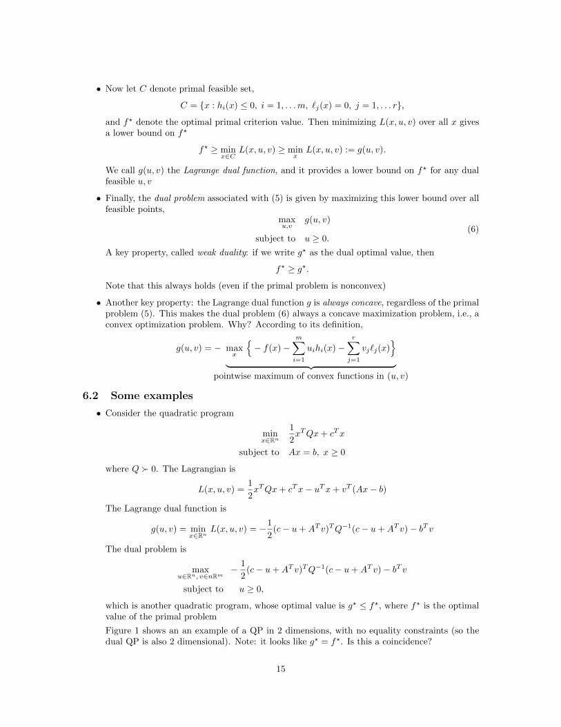
Figure 1 shows an an example of a QP in 2 dimensions, with no equality constraints (so thedual QP is also 2 dimensional). Note: it looks like g? = f?. Is this a coincidence?

15

x1 / u1 x2 / u2

f / g

●●

primal

dual

Figure 1: The primal and dual criterion surfaces for the quadratic minimization example.

• As another example, consider the quartic minimization problem

minx∈R

x4 − 50x2 + 100x

subject to x ≥ −4.5.

This is nonconvex (because its criterion is nonconvex). Although it is a pretty messy calcula-tion, here the dual function g can be derived explicitly (via the analytic formula for roots of acubic equation):

g(u) = mini=1,2,3

F 4i (u)− 50F 2

i (u) + 100Fi(u),

where for i = 1, 2, 3,

Fi(u) =−ai

12 · 21/3

(432(100− u)−

(4322(100− u)2 − 4 · 12003

)1/2)1/3

−

100 · 21/3 1(432(100− u)−

(4322(100− u)2 − 4 · 12003

)1/2)1/3,

and a1 = 1, a2 = (−1 + i√

3)/2, a3 = (−1− i√

3)/2. Without the context of duality it wouldbe difficult to tell whether or not g is concave ... but we know it must be!

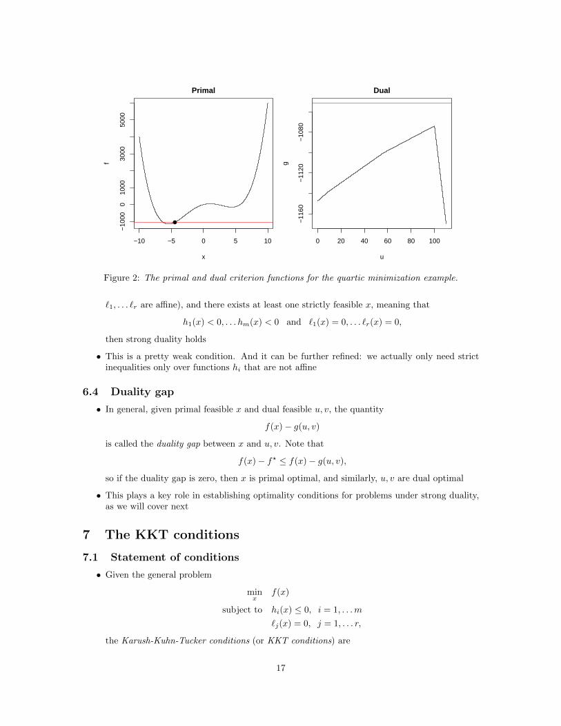
Figure 2 displays the primal and dual criterion functions for this quartic example. Note: it isevident that g? < f?, i.e., the lower bound constructed from the dual problem is strictly lessthan the primal optimal value. Why?

6.3 Strong duality and Slater’s condition

• We have seen an example above in which the dual problem delivers a tight lower bound, inthat g? = f?; this phenomenon is called strong duality

• When does strong duality this hold in general? A sufficient (but not necessary) condition iscalled Slater’s condition: if the primal problem (5) is a convex (i.e., f, h1, . . . hm are convex,

16

−10 −5 0 5 10

−10

000

1000

3000

5000

Primal

x

f

●

0 20 40 60 80 100

−11

60−

1120

−10

80

Dual

u

gFigure 2: The primal and dual criterion functions for the quartic minimization example.

`1, . . . `r are affine), and there exists at least one strictly feasible x, meaning that

h1(x) < 0, . . . hm(x) < 0 and `1(x) = 0, . . . `r(x) = 0,

then strong duality holds

• This is a pretty weak condition. And it can be further refined: we actually only need strictinequalities only over functions hi that are not affine

6.4 Duality gap

• In general, given primal feasible x and dual feasible u, v, the quantity

f(x)− g(u, v)

is called the duality gap between x and u, v. Note that

f(x)− f? ≤ f(x)− g(u, v),

so if the duality gap is zero, then x is primal optimal, and similarly, u, v are dual optimal

• This plays a key role in establishing optimality conditions for problems under strong duality,as we will cover next

7 The KKT conditions

7.1 Statement of conditions

• Given the general problem

minx

f(x)

subject to hi(x) ≤ 0, i = 1, . . .m

`j(x) = 0, j = 1, . . . r,

the Karush-Kuhn-Tucker conditions (or KKT conditions) are

17

– 0 ∈ ∂f(x) +∑mi=1 ui∂hi(x) +

∑rj=1 vj∂`j(x) (stationarity)

– ui · hi(x) = 0 for all i = 1, . . .m (complementary slackness)

– hi(x) ≤ 0, `j(x) = 0 for all i = 1, . . .m, j = 1, . . . r (primal feasibility)

– ui ≥ 0 for all i = 1, . . .m (dual feasibility)

Note that the KKT conditions are a statement about a triplet of variables x, u, v, where x isa primal variable, and u, v are dual variables, i.e., u, v are associated with the dual problem

maxu,v

g(u, v)

subject to u ≥ 0.

But importantly, we don’t to need to form the dual function g to examine the KKT conditions

7.2 Necessity

• Let x? and u?, v? be primal and dual solutions with zero duality gap (this means that strongduality holds, e.g., under Slater’s condition). Then the KKT conditions must hold

• Proof: we have

f(x?) = g(u?, v?)

= minx

f(x) +

m∑i=1

u?i hi(x) +

r∑j=1

v?j `j(x)

≤ f(x?) +

m∑i=1

u?i hi(x?) +

r∑j=1

v?j `j(x?)

≤ f(x?).

In other words, all these inequalities are actually equalities. Two things to learn from this:

1. The point x? minimizes L(x, u?, v?) over x ∈ Rn. Hence the subdifferential of L(x, u?, v?)must contain 0 at x = x?; this is exactly the stationarity condition

2. We must have∑mi=1 u

?i hi(x

?) = 0, and because each term here is ≤ 0, this implies thatu?i hi(x

?) = 0 for i = 1, . . .m; this is exactly complementary slackness

Primal and dual feasibility obviously hold. Hence, we’ve verified the KKT conditions

• For this direction of the problem, we have assumed nothing a priori about the convexity of ouroptimization problem; we have rather assumed strong duality (a zero duality gap) directly

7.3 Sufficiency

• Suppose that x?, u?, v? satisfy the KKT conditions. Then x? is a primal solution and u?, v? isa dual solution

• Proof: we have

g(u?, v?) = f(x?) +

m∑i=1

u?i hi(x?) +

r∑j=1

v?j `j(x?)

= f(x?)

where the first equality holds from the stationarity condition, and the second equality holdsfrom complementary slackness and primal feasibility. Therefore the duality gap is zero (andx? and u?, v? are primal and dual feasible) so x? and u?, v? are primal and dual optimal

18

7.4 Putting it together

• The KKT conditions are always sufficient for optimality, and necessary under strong duality

• Hence, for a problem with strong duality—e.g., under Slater’s condition: the problem is convexand there exists a point x strictly satisfying its nonaffine inequality contraints—we have

x? and u?, v? are primal and dual solutions

⇐⇒ x? and u?, v? satisfy the KKT conditions

• A warning, concerning the stationarity condition: for a differentiable function f , we do notknow that ∂f(x) = {∇f(x)} unless f is convex. This is a common mistake!

7.5 Some examples

• Consider for Q � 0, the quadratic program

minx∈Rn

1

2xTQx+ cTx

subject to Ax = 0

This is a convex problem, with no inequality constraints, so by the KKT conditions: x is asolution if and only if [

Q AT

A 0

] [xu

]=

[−c0

]for some u. Linear system combines stationarity, primal feasibility (complementary slacknessand dual feasibility are vacuous)

• When the primal problem convex, and unconstrained, the KKT conditions are necessary andsufficient for optimality. But in this case, the KKT conditions just reduce to the stationaritycondition:

0 ∈ ∂f(x),

which we already know is necessary and sufficient for optimality, from the subgradient char-acterization

• Consider the `1 penalized problem

minβ∈Rp

f(Xβ) + λ‖β‖1,

where f : Rn → R is a convex, differentiable function, and X ∈ Rn×p is a matrix of predictors(columns) X1, . . . Xp ∈ Rn. This problem is convex and unconstrained, so the stationaritycondition is necessary and sufficient for optimality, which is

−XT∇f(Xβ) = λs,

where s ∈ ∂‖β‖1, i.e.,

si ∈

{1} if βi > 0

{−1} if βi < 0

[−1, 1] if βi = 0.

Now we can read off an important fact: if |XTi ∇f(Xβ)| < λ, then βi = 0

19

• Consider the graphical lasso problem

minΘ∈Sp++

− log det Θ + tr(SΘ) + λ‖Θ‖1,

where S ∈ Sp+ is a positive semidefinite sample covariance matrix, and ‖Θ‖1 =∑pi,j=1 |Θij |.

The KKT conditions again reduce to the stationary condition,

−Θ−1 + S + Γ = 0,

where Γ ∈ Rp×p has elements Γij ∈ ∂|Θij |, i.e.,

Γij ∈

{1} if Θij > 0

{−1} if Θij < 0

[−1, 1] if Θij = 0.

This stationarity condition actually tells us whole lot about the structure of Θ at optimality.Let S denote the componentwise soft-thresholded version of S, i.e., with components

Sij =

Sij − λ if Sij > λ

0 if − λ ≤ Sij ≤ λSij + λ if Sij < −λ

.

Observe:

– If Θ is block diagonal, then so is Θ−1, with the same block structure. Hence, for all i, jin different blocks, we must have |Sij | ≤ λ, so S has the same block structure

– If S is block diagonal, then the stationarity condition is satisfied with Γij = 0 for all i, jin different blocks, and Θ−1 block diagonal. Hence Θ has the same block structure

Therefore, we have shown that the block structure of the minimizer Θ is exactly the same asthe block structure of S, the thresholded sample covariance matrix. This makes the graphicallasso look very simple-minded, in a way!

7.6 Constrained and Lagrange forms

• Often in statistics and machine learning, we’ll switch back and forth between the constrainedform of a problem, where t ∈ R is a tuning parameter,

minx

f(x) subject to h(x) ≤ t, (C)

and the Lagrange form, where λ ≥ 0 is a tuning parameter,

minx

f(x) + λ · h(x), (L)

and claim these are equivalent. Is this true (assuming convex f, h)?

• (C) to (L): if problem (C) is strictly feasible, then strong duality holds, and there exists someλ ≥ 0 (dual solution) such that any solution x? in (C) minimizes

f(x) + λ · (h(x)− t),

so x? is also a solution in (L)

20

• (L) to (C): if x? is a solution in (L), then the KKT conditions for (C) are satisfied by takingt = h(x?), so x? is a solution in (C)

• Conclusion: ⋃λ≥0

{solutions in (L)} ⊆⋃t

{solutions in (C)}⋃λ≥0

{solutions in (L)} ⊇⋃

t such that (C)is strictly feasible

{solutions in (C)}

Strictly speaking this is not a perfect equivalence (albeit minor nonequivalence). Note: whenthe only value of t that leads to a feasible but not strictly feasible constraint set is t = 0, i.e.,

{x : h(x) ≤ t} 6= ∅, {x : h(x) < t} = ∅ =⇒ t = 0

(e.g., this is true if g is a norm), then we do get perfect equivalence

7.7 Solving the primal via the dual

• Recall that under strong duality, given dual optimal u?, v?, any primal solution minimizesL(x, u?, v?) over x (it satisfies the stationarity condition). In other words, any primal solutionx? solves

minx

f(x) +

m∑i=1

u?i hi(x) +

r∑j=1

v?i `j(x).

Often, solutions of this unconstrained problem can be expressed explicitly, giving an explicitcharacterization of primal solutions from dual solutions

• As an exmaple, consider the lasso problem

minβ∈Rp

1

2‖y −Xβ‖22 + λ‖β‖1.

Its dual function is just a constant (equal to f?). Hence we reparametrize the primal problem

minβ∈Rp, z∈Rn

1

2‖y − z‖22 + λ‖β‖1 subject to z = Xβ,

so the dual function is now

g(u) = minβ∈Rp, z∈Rn

1

2‖y − z‖22 + λ‖β‖1 + uT (z −Xβ)

=1

2‖y‖22 + min

z∈Rn

(1

2‖z‖22 − (y − u)T z

)+ minβ∈Rp

(λ‖β‖1 − (XTu)Tβ

)=

1

2‖y‖22 −

1

2‖y − u‖22 − I

{‖XTu‖∞ ≤ λ

}.

Above, we used the fact that the minimum over β is −∞ if ‖XTu‖∞ > λ, and 0 otherwise.Therefore, the lasso dual is

maxu∈Rn

1

2

(‖y‖22 − ‖y − u‖22

)subject to ‖XTu‖∞ ≤ λ,

or equivalentlyminu∈Rn

‖y − u‖22 subject to ‖XTu‖∞ ≤ λ.

21

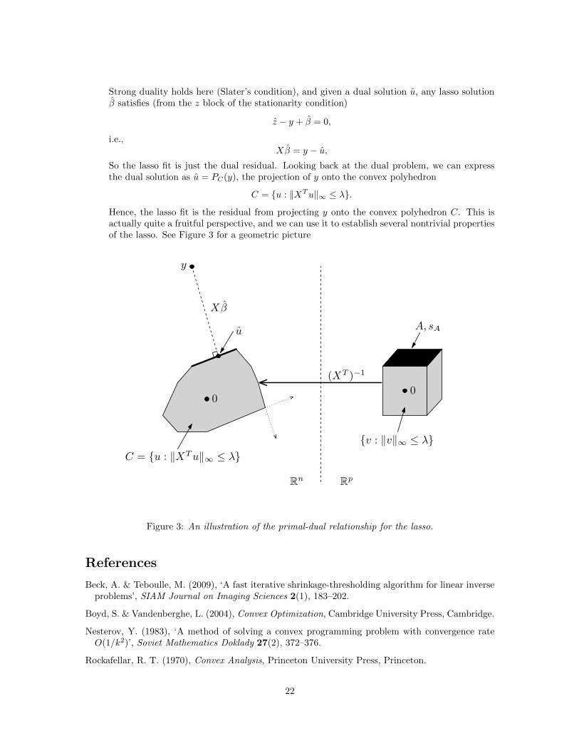
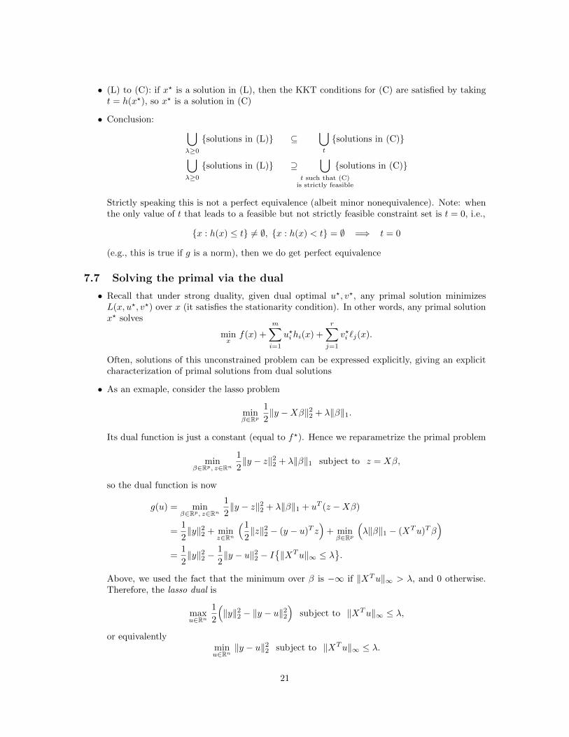
Strong duality holds here (Slater’s condition), and given a dual solution u, any lasso solutionβ satisfies (from the z block of the stationarity condition)

z − y + β = 0,

i.e.,Xβ = y − u,

So the lasso fit is just the dual residual. Looking back at the dual problem, we can expressthe dual solution as u = PC(y), the projection of y onto the convex polyhedron

C = {u : ‖XTu‖∞ ≤ λ}.Hence, the lasso fit is the residual from projecting y onto the convex polyhedron C. This isactually quite a fruitful perspective, and we can use it to establish several nontrivial propertiesof the lasso. See Figure 3 for a geometric picture

y

C = {u : ‖XTu‖∞ ≤ λ}

Xβ

00

u

{v : ‖v‖∞ ≤ λ}

A, sA

(XT )−1

Rn Rp

1

Figure 3: An illustration of the primal-dual relationship for the lasso.

References

Beck, A. & Teboulle, M. (2009), ‘A fast iterative shrinkage-thresholding algorithm for linear inverseproblems’, SIAM Journal on Imaging Sciences 2(1), 183–202.

Boyd, S. & Vandenberghe, L. (2004), Convex Optimization, Cambridge University Press, Cambridge.

Nesterov, Y. (1983), ‘A method of solving a convex programming problem with convergence rateO(1/k2)’, Soviet Mathematics Doklady 27(2), 372–376.

Rockafellar, R. T. (1970), Convex Analysis, Princeton University Press, Princeton.

22