Embed Size (px)
Citation preview

Copyright
by
James Stephen Doran
2004

The Dissertation Committee for James Stephen Dorancertifies that this is the approved version of the following dissertation:
On the Market Price of Volatility Risk
Committee:
Ehud Ronn, Supervisor
Stephen Magee
Ramesh Rao
Stathis Tompaidis
Li Gan
On the Market Price of Volatility Risk
by
James Stephen Doran, B.A.
DISSERTATION
Presented to the Faculty of the Graduate School of
The University of Texas at Austin
in Partial Fulfillment
of the Requirements
for the Degree of
DOCTOR OF PHILOSOPHY
THE UNIVERSITY OF TEXAS AT AUSTIN
May 2004

Dedicated to my wife Heather, my parents Charles and Elaine, and to my
son Jackson.

Acknowledgments
I wish to thank the multitudes of people who helped me.
I would like to single out especially my advisor, Ehud Ronn, my parents,
Charles and Elaine, and my wife Heather
This work would never have to come to fruition without the guidance and
support of my advisor and friend Ehud Ronn. His persistence and belief in me
was the necessary and sufficient condition required for successful completion
of this document.
Without the words of wisdom and teaching of my parents, I would never have
persisted in the pursuit of my goals, from the smallest task to the largest
achievement.
Finally, if it had not been for my wife, with which all things begin and end, I
would never have been at this stage in life that I am at today. It is our lives
together that allow us individually to succeed.
. . .
v
On the Market Price of Volatility Risk
Publication No.
James Stephen Doran, Ph.D.
The University of Texas at Austin, 2004
Supervisor: Ehud Ronn
This work examines the extent of the bias between Black-Scholes (1973)/Black
(1976) implied volatility and realized term volatility, estimation of the market
price of volatility risk, and option model fit in the natural gas market. To
examine this bias I institute a stochastic volatility data generating process,
and demonstrate the bias through Monte Carlo simulation of the underlying
parameters. This provides a numerical justification for testing the importance
of a risk premia for volatility. I implement empirical tests for the market
price of volatility risk by analyzing at-the-money options on the S&P 500 and
S&P 100. Further, I extend the study by considering options on natural gas
contracts by examining option model fit for a variety of parametric candi-
dates. Using risk-neutral parameter estimates I re-estimate the market price
of volatility risk using the full cross-section of option prices. The findings
demonstrate a negative market price of volatility risk, and show that this risk
is a significant component of the bias between Black-Scholes/Black implied
volatility and realized term volatility.
vi
Table of Contents
Acknowledgments v
Abstract vi
List of Tables x
List of Figures xiii
Chapter 1. Introduction 1
1.1 Evidence on the Market Price of Volatility Risk . . . . . . . . 9
Chapter 2. The Bias in Black-Scholes/BlackImplied Volatility 14
2.1 Introduction . . . . . . . . . . . . . . . . . . . . . . . . . . . . 14
2.2 The Model . . . . . . . . . . . . . . . . . . . . . . . . . . . . . 14
2.2.1 Stochastic Volatility . . . . . . . . . . . . . . . . . . . . 14
2.3 Estimation of the Bias in BSIV/BIV . . . . . . . . . . . . . . . 19
2.3.1 Data . . . . . . . . . . . . . . . . . . . . . . . . . . . . 19
2.3.1.1 Measurement Error . . . . . . . . . . . . . . . . 21
2.3.2 Estimating the bias . . . . . . . . . . . . . . . . . . . . 22
2.3.2.1 Equity Bias . . . . . . . . . . . . . . . . . . . . 22
2.3.2.2 Modeling of the TSOV . . . . . . . . . . . . . . 26
2.3.2.3 Gas Bias . . . . . . . . . . . . . . . . . . . . . . 30
2.4 Conclusion . . . . . . . . . . . . . . . . . . . . . . . . . . . . . 35
Chapter 3. Monte Carlo Simulation and Estimation of the Mar-ket Price of Volatility Risk 36
3.1 Introduction . . . . . . . . . . . . . . . . . . . . . . . . . . . . 36
3.2 Monte Carlo Simulation . . . . . . . . . . . . . . . . . . . . . . 37
vii
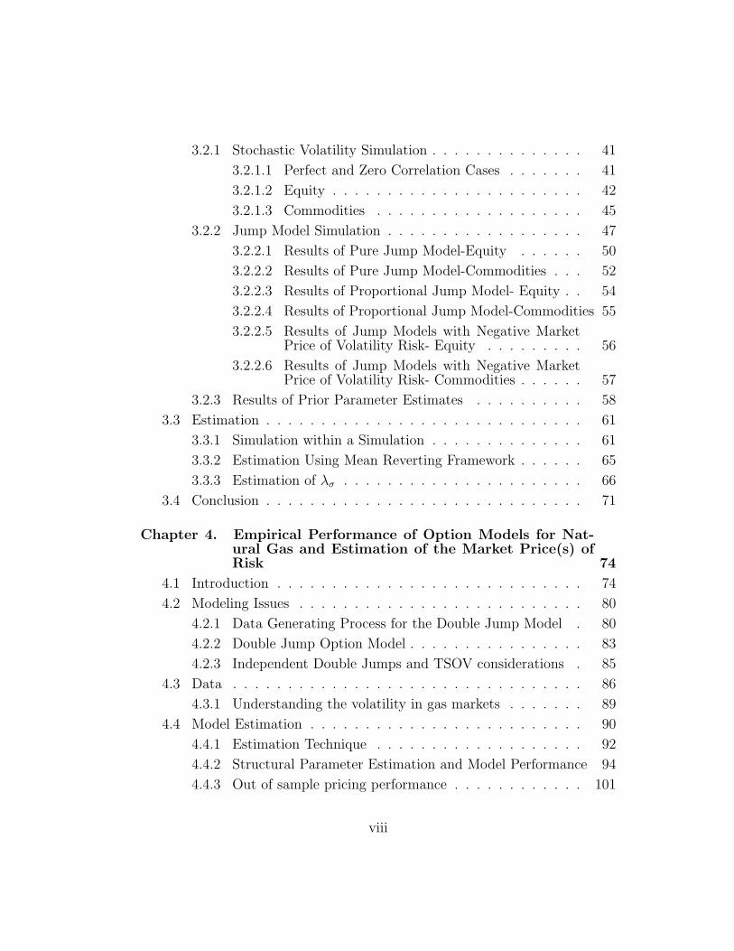
3.2.1 Stochastic Volatility Simulation . . . . . . . . . . . . . . 41
3.2.1.1 Perfect and Zero Correlation Cases . . . . . . . 41
3.2.1.2 Equity . . . . . . . . . . . . . . . . . . . . . . . 42
3.2.1.3 Commodities . . . . . . . . . . . . . . . . . . . 45
3.2.2 Jump Model Simulation . . . . . . . . . . . . . . . . . . 47
3.2.2.1 Results of Pure Jump Model-Equity . . . . . . 50
3.2.2.2 Results of Pure Jump Model-Commodities . . . 52
3.2.2.3 Results of Proportional Jump Model- Equity . . 54
3.2.2.4 Results of Proportional Jump Model-Commodities 55
3.2.2.5 Results of Jump Models with Negative MarketPrice of Volatility Risk- Equity . . . . . . . . . 56
3.2.2.6 Results of Jump Models with Negative MarketPrice of Volatility Risk- Commodities . . . . . . 57
3.2.3 Results of Prior Parameter Estimates . . . . . . . . . . 58
3.3 Estimation . . . . . . . . . . . . . . . . . . . . . . . . . . . . . 61
3.3.1 Simulation within a Simulation . . . . . . . . . . . . . . 61
3.3.2 Estimation Using Mean Reverting Framework . . . . . . 65
3.3.3 Estimation of λσ . . . . . . . . . . . . . . . . . . . . . . 66
3.4 Conclusion . . . . . . . . . . . . . . . . . . . . . . . . . . . . . 71
Chapter 4. Empirical Performance of Option Models for Nat-ural Gas and Estimation of the Market Price(s) ofRisk 74
4.1 Introduction . . . . . . . . . . . . . . . . . . . . . . . . . . . . 74
4.2 Modeling Issues . . . . . . . . . . . . . . . . . . . . . . . . . . 80
4.2.1 Data Generating Process for the Double Jump Model . 80
4.2.2 Double Jump Option Model . . . . . . . . . . . . . . . . 83
4.2.3 Independent Double Jumps and TSOV considerations . 85
4.3 Data . . . . . . . . . . . . . . . . . . . . . . . . . . . . . . . . 86
4.3.1 Understanding the volatility in gas markets . . . . . . . 89
4.4 Model Estimation . . . . . . . . . . . . . . . . . . . . . . . . . 90
4.4.1 Estimation Technique . . . . . . . . . . . . . . . . . . . 92
4.4.2 Structural Parameter Estimation and Model Performance 94
4.4.3 Out of sample pricing performance . . . . . . . . . . . . 101
viii
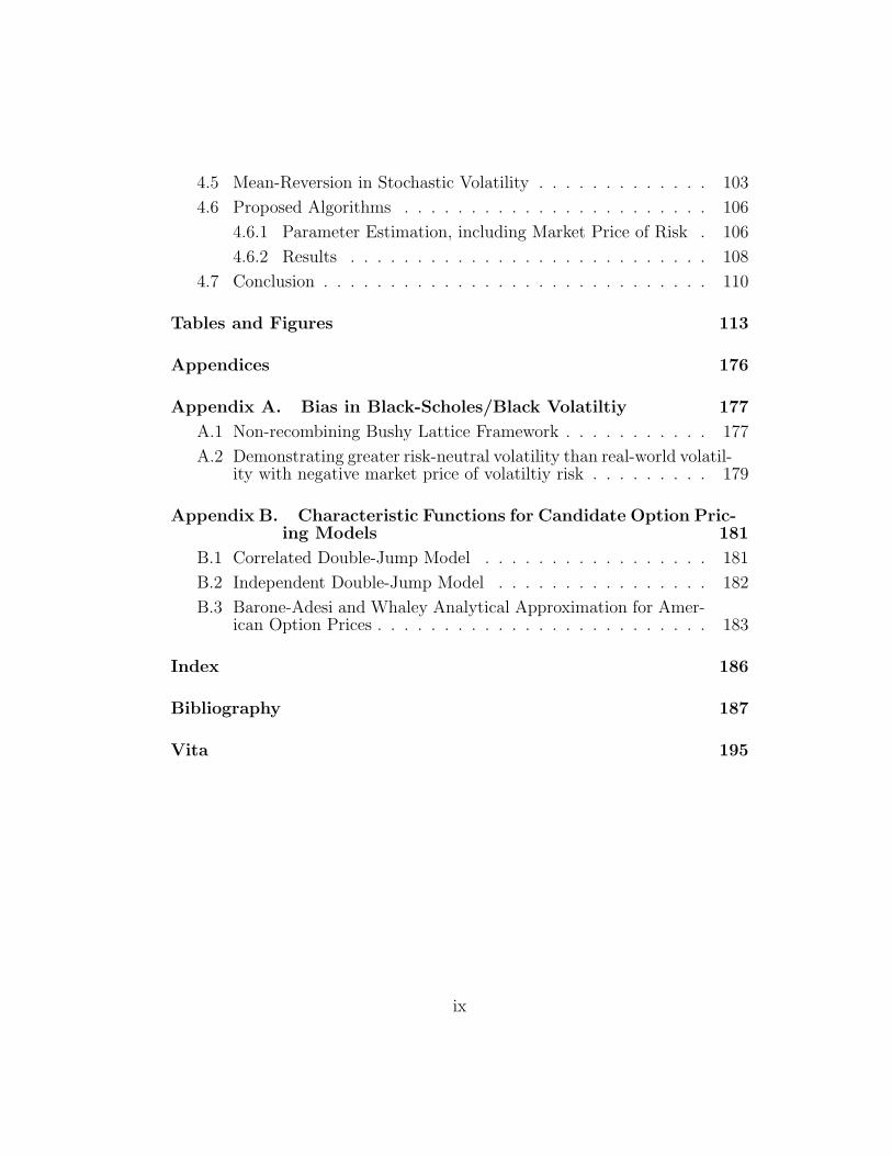
4.5 Mean-Reversion in Stochastic Volatility . . . . . . . . . . . . . 103
4.6 Proposed Algorithms . . . . . . . . . . . . . . . . . . . . . . . 106
4.6.1 Parameter Estimation, including Market Price of Risk . 106
4.6.2 Results . . . . . . . . . . . . . . . . . . . . . . . . . . . 108
4.7 Conclusion . . . . . . . . . . . . . . . . . . . . . . . . . . . . . 110
Tables and Figures 113
Appendices 176
Appendix A. Bias in Black-Scholes/Black Volatiltiy 177
A.1 Non-recombining Bushy Lattice Framework . . . . . . . . . . . 177
A.2 Demonstrating greater risk-neutral volatility than real-world volatil-ity with negative market price of volatiltiy risk . . . . . . . . . 179
Appendix B. Characteristic Functions for Candidate Option Pric-ing Models 181
B.1 Correlated Double-Jump Model . . . . . . . . . . . . . . . . . 181
B.2 Independent Double-Jump Model . . . . . . . . . . . . . . . . 182
B.3 Barone-Adesi and Whaley Analytical Approximation for Amer-ican Option Prices . . . . . . . . . . . . . . . . . . . . . . . . . 183
Index 186
Bibliography 187
Vita 195
ix
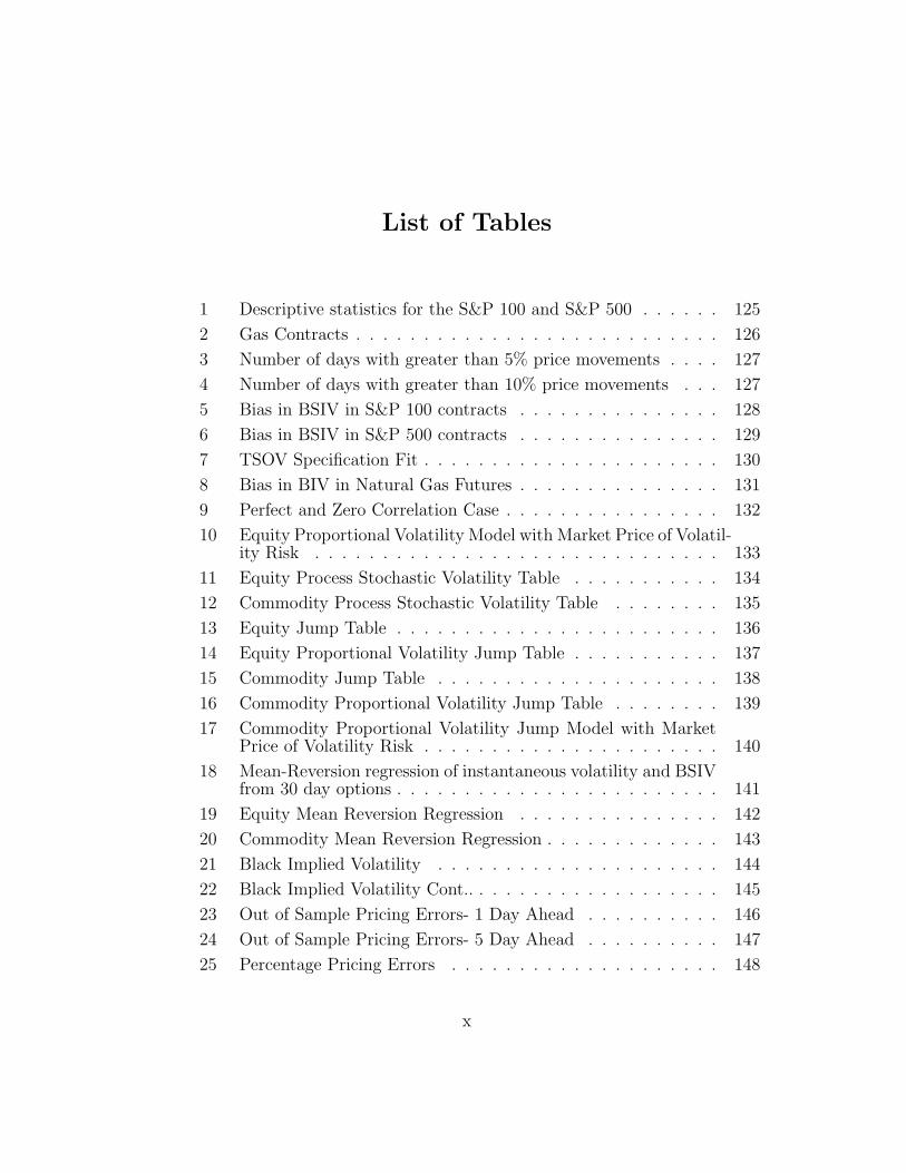
List of Tables
1 Descriptive statistics for the S&P 100 and S&P 500 . . . . . . 125
2 Gas Contracts . . . . . . . . . . . . . . . . . . . . . . . . . . . 126
3 Number of days with greater than 5% price movements . . . . 127
4 Number of days with greater than 10% price movements . . . 127
5 Bias in BSIV in S&P 100 contracts . . . . . . . . . . . . . . . 128
6 Bias in BSIV in S&P 500 contracts . . . . . . . . . . . . . . . 129
7 TSOV Specification Fit . . . . . . . . . . . . . . . . . . . . . . 130
8 Bias in BIV in Natural Gas Futures . . . . . . . . . . . . . . . 131
9 Perfect and Zero Correlation Case . . . . . . . . . . . . . . . . 132
10 Equity Proportional Volatility Model with Market Price of Volatil-ity Risk . . . . . . . . . . . . . . . . . . . . . . . . . . . . . . 133
11 Equity Process Stochastic Volatility Table . . . . . . . . . . . 134
12 Commodity Process Stochastic Volatility Table . . . . . . . . 135
13 Equity Jump Table . . . . . . . . . . . . . . . . . . . . . . . . 136
14 Equity Proportional Volatility Jump Table . . . . . . . . . . . 137
15 Commodity Jump Table . . . . . . . . . . . . . . . . . . . . . 138
16 Commodity Proportional Volatility Jump Table . . . . . . . . 139
17 Commodity Proportional Volatility Jump Model with MarketPrice of Volatility Risk . . . . . . . . . . . . . . . . . . . . . . 140
18 Mean-Reversion regression of instantaneous volatility and BSIVfrom 30 day options . . . . . . . . . . . . . . . . . . . . . . . . 141
19 Equity Mean Reversion Regression . . . . . . . . . . . . . . . 142
20 Commodity Mean Reversion Regression . . . . . . . . . . . . . 143
21 Black Implied Volatility . . . . . . . . . . . . . . . . . . . . . 144
22 Black Implied Volatility Cont.. . . . . . . . . . . . . . . . . . . 145
23 Out of Sample Pricing Errors- 1 Day Ahead . . . . . . . . . . 146
24 Out of Sample Pricing Errors- 5 Day Ahead . . . . . . . . . . 147
25 Percentage Pricing Errors . . . . . . . . . . . . . . . . . . . . 148
x
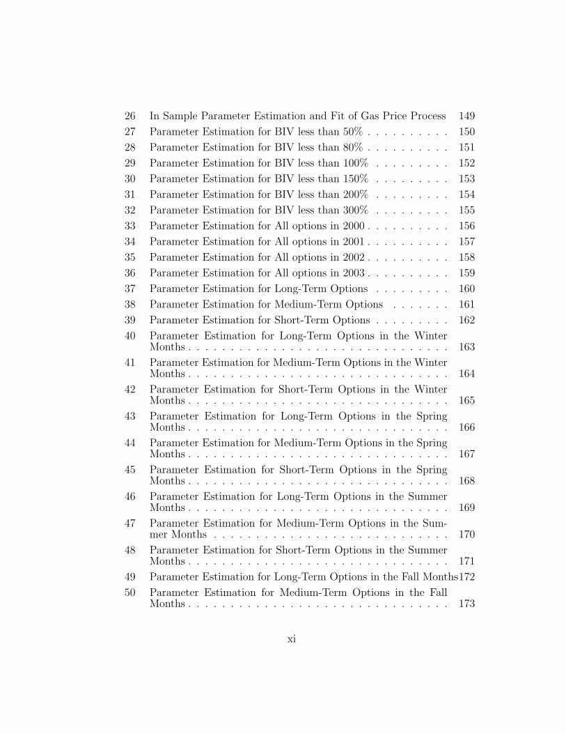
26 In Sample Parameter Estimation and Fit of Gas Price Process 149
27 Parameter Estimation for BIV less than 50% . . . . . . . . . . 150
28 Parameter Estimation for BIV less than 80% . . . . . . . . . . 151
29 Parameter Estimation for BIV less than 100% . . . . . . . . . 152
30 Parameter Estimation for BIV less than 150% . . . . . . . . . 153
31 Parameter Estimation for BIV less than 200% . . . . . . . . . 154
32 Parameter Estimation for BIV less than 300% . . . . . . . . . 155
33 Parameter Estimation for All options in 2000 . . . . . . . . . . 156
34 Parameter Estimation for All options in 2001 . . . . . . . . . . 157
35 Parameter Estimation for All options in 2002 . . . . . . . . . . 158
36 Parameter Estimation for All options in 2003 . . . . . . . . . . 159
37 Parameter Estimation for Long-Term Options . . . . . . . . . 160
38 Parameter Estimation for Medium-Term Options . . . . . . . 161
39 Parameter Estimation for Short-Term Options . . . . . . . . . 162
40 Parameter Estimation for Long-Term Options in the WinterMonths . . . . . . . . . . . . . . . . . . . . . . . . . . . . . . . 163
41 Parameter Estimation for Medium-Term Options in the WinterMonths . . . . . . . . . . . . . . . . . . . . . . . . . . . . . . . 164
42 Parameter Estimation for Short-Term Options in the WinterMonths . . . . . . . . . . . . . . . . . . . . . . . . . . . . . . . 165
43 Parameter Estimation for Long-Term Options in the SpringMonths . . . . . . . . . . . . . . . . . . . . . . . . . . . . . . . 166
44 Parameter Estimation for Medium-Term Options in the SpringMonths . . . . . . . . . . . . . . . . . . . . . . . . . . . . . . . 167
45 Parameter Estimation for Short-Term Options in the SpringMonths . . . . . . . . . . . . . . . . . . . . . . . . . . . . . . . 168
46 Parameter Estimation for Long-Term Options in the SummerMonths . . . . . . . . . . . . . . . . . . . . . . . . . . . . . . . 169
47 Parameter Estimation for Medium-Term Options in the Sum-mer Months . . . . . . . . . . . . . . . . . . . . . . . . . . . . 170
48 Parameter Estimation for Short-Term Options in the SummerMonths . . . . . . . . . . . . . . . . . . . . . . . . . . . . . . . 171
49 Parameter Estimation for Long-Term Options in the Fall Months172
50 Parameter Estimation for Medium-Term Options in the FallMonths . . . . . . . . . . . . . . . . . . . . . . . . . . . . . . . 173
xi

51 Parameter Estimation for Short-Term Options in the Fall Months174
52 Market Price(s) of Risk . . . . . . . . . . . . . . . . . . . . . . 175
xii

List of Figures
1 Cross-sectional model comparision . . . . . . . . . . . . . . . . 114
2 VIX index . . . . . . . . . . . . . . . . . . . . . . . . . . . . . 115
3 TSOV . . . . . . . . . . . . . . . . . . . . . . . . . . . . . . . 116
4 January Natural Gas Contracts Implied Volatility . . . . . . . 117
5 August Natural Gas Contracts Implied Volatility . . . . . . . 118
6 Cross-section BSIV plots . . . . . . . . . . . . . . . . . . . . . 119
7 Cross-section BIV plots . . . . . . . . . . . . . . . . . . . . . . 120
8 Simulation within a simulation technique . . . . . . . . . . . . 121
9 BIV plots for long-term 2001 contracts . . . . . . . . . . . . . 122
10 BIV plots for long-term 2002 contracts . . . . . . . . . . . . . 122
11 BIV plots for medium-term 2001 contracts . . . . . . . . . . . 123
12 BIV plots for medium-term 2002 contracts . . . . . . . . . . . 123
13 BIV plots for short-term 2001 contracts . . . . . . . . . . . . . 124
14 BIV plots for short-term 2002 contracts . . . . . . . . . . . . . 124
xiii

Chapter 1
Introduction
To what extent is implied volatility a biased or unbiased predictor of
future realized volatility? The answer to this question is important for a
variety of reasons, impacting option trading, volatility forecasting, and overall
risk management. Understanding this bias could lead to resolving issues such
as why option traders tend to be short and whether forward prices are upward-
or downward-biased predictors of spot prices. The predictive power of implied
volatility will be explored in both the equity and commodity markets, as one
of my objectives in this work is to understand this bias.
There exists a rich literature on the computation and interpretation
of implied volatility, following closely upon the heels of the derivation of the
Black-Scholes option pricing formula. Christensen and Prabhala (1998) com-
pared implied volatility to an ex-post estimate of return volatility. By per-
forming a time-series analysis of pre- and post-87 data, they suggest that the
implied volatility of S&P 100 index options is an unbiased and efficient predic-
tor of future volatility. They were able to show that implied volatility remains
an efficient estimator even when including past volatility in the specification.
Others, such as Jorion (1995) and Lamoureux and Lastrapes (1993), consid-
1
ered foreign currency options and have suggested that implied volatility, while
efficient, is a biased predictor of future realized volatility.
If Black-Scholes implied volatility is truly an unbiased predictor of fu-
ture realized term volatility, this is consistent with the hypothesis that the
Black-Scholes model is the “true” model for stock prices, and that there is
no model misspecification. Such a conclusion would appear inconsistent with
the volatility skew present in option prices. In fact, we should expect Black-
Scholes/Black implied volatility to be biased, when we account for the market
price of volatility risk within a jump and/or stochastic volatility framework.
The estimation will lead to the conclusion that Black-Scholes implied volatil-
ity is an upward-biased predictor, which I will relate to the underlying data
generating process.
The evolution of the commodity markets differs from the tradition eq-
uity/index markets, and reporting on the volatility bias and underlying pa-
rameters in this market is the next objective. I will use Black’s formula for
the implied volatility (BIV) for the commodity simulation case. Commodities
contracts add additional complexity not prevalent for equities. The presence
of a significant term structure of volatility (TSOV), as well as seasonality, re-
quires additional modeling, and further complicates estimation. Thus I resort
to estimating the necessary TSOV parameters that reduce pricing errors by
postulating three parametric forms for the term structure. The findings sug-
gest that a reciprocal specification for the TSOV best fits the model when
there is a severe “ramping up” of volatility, versus the traditional Schwartz
2

(1997) specification and a quadratic form. As for seasonality, it was necessary
to separate the contracts by months. This allows further insight into the effects
of stochastic volatility premiums on winter versus summer months. There is
an additional concern with liquidity issues, and/or sticky prices, due to low
turnover. Focusing on gas contracts versus oil or electricity, minimized these
concerns since the volume is sufficient and data is readily available. After
accounting for these idosyncrasies, demonstrating BIV is an upward-bias pre-
dictor of future realized volatility can be accomplished in similar methodology
to the upward-bias in BSIV.
After estimation, the intent is to examine current option pricing models
to determine how well each model can explain this bias. Whereas Black and
Scholes (1973) postulated a geometric Brownian motion, papers such as Hull
and White (1987), Heston (1993), and Bates (1994, 1996) introduced stochas-
tic volatility and jumps into the data generating process, with the intended
implication that prices may incorporate premiums for jumps and changes in
volatility. Incorporating both stochastic volatility and jumps in the formu-
lation, I consider the individual and combined effects of the underlying pa-
rameters and how they either contribute to, or diminish, the bias in implied
volatility.
Recent literature has expanded upon these models by incorporating
additional factors such as jumps in volatility, multiple volatility factors, and
alternative power coefficients. While these models help improve the under-
standing of the evolution of options markets, there are unanswered questions
3

that can be resolved without the need for such additional price-process model-
ing. In addition, there appears to be limited significant improvement to overall
model fit.1
The parameter of particular interest is the market price of volatility risk.
There is a wide body of literature on stochastic volatility models, but very lim-
ited information on the market price of volatility risk. Only recently, findings
in Bakshi and Kapadia (2001), Coval and Shumway (2001), Pan (2000), and
others address the direction and magnitude of market price of volatility risk.
The hypothesis is that the market price of volatility risk is indelibly linked
to the bias in Black-Scholes implied volatility: The process volatility and in-
teraction with the market price of volatility risk, determines the magnitude
of the bias. If market price of volatility risk is negative, this can potentially
explain the upward-bias we observe in Black-Scholes implied volatility as well
as contribute to Bates’ (1996) finding that out-of-the money (OTM) puts are
volatility skew expensive relative to other options. Traders short OTM puts
require compensation for volatility risk, independent of any jump intensity or
jump size risk that may also be included. Eraker (2001) and Bates (2000)
have documented the Sharpe ratios of OTM puts are approximately six times
higher than the Sharpe ratio of traditional equity portfolios. These results
suggest large premiums for exposure to volatility risk. However, fully under-
standing this parameter requires going beyond examining volatility changes
1A test of the double-jump model of Duffie, Pan, and Singelton (2002) performed by Bak-shi and Cao (2003), reveals no significant difference between this model and the traditionalstochastic volatility with jump model in terms of RMSE
4

through time. It is necessary to examine this parameter in conjunction with
jumps in the price process, since these are two separate effects. Regardless
of model specification, inferring significant estimates for the parameter is a
non-trivial exercise, that requires either extensive years of data or advanced
econometric techniques.
The commodity market is quite distinct from the equity market. First,
individuals are net consumers of energy, versus net savers in the equity mar-
ket. Secondly, forward prices may be upward-bias predictors of expected spot
prices in the energy markets while the reverse is true for equities.2 Third, we
observe implied volatility skews for out-of-the money calls and in-the-money
puts; this is possibly due to firms wishing to hedge against energy market price
spikes/positive jumps. This may suggest a positive market price of volatility
risk for energy commodities. However, if forward prices are upward-bias pre-
dictors of expected spot prices, it implies a negative market price of risk for
energy products.3 A positive skew, which is a possible indicator of positive
correlation between the price and volatility process, also leads to the conclu-
sion that the market price of volatility risk is negative, as it is in the equity
markets. Nevertheless, it is not clear that the market price of risk is negative in
commodity markets, and thus the claim that there are negative Sharpe ratios
for energy commodities is debatable. Through the estimation of a negative
market price of volatility risk for the gas markets, and establishing positive
2Since the expected rate of return is typically higher for equities than the risk free rate,one expects that forward prices are downward bias predictors of expected spot prices.
3As noted by Dincerler and Ronn (2001)
5

correlation between price and volatility, strengthens the argument for negative
values for the market price of risk in commodities. In addition, I can relate
the upward-bias predictive nature in BIV by showing that it necessary to have
a negative market price of volatility risk.
Central to the estimation for the market price of volatility risk is relat-
ing the bias in Black-Scholes/Black implied volatility to the underlying data
generating process. Accomplishing estimation required recovering the risk neu-
tral parameters by linking the instantaneous volatility to thirty day BSIV/BIV
through a simulation technique. Recent literature has focused on the appro-
priate way to estimate continuous time models. Chernov and Ghysels (2002)
use the Galant and Tauchen EMM technique, Pan (2000) applied an IS-GMM
framework, and Jones (2001)and Eraker (2001) have used Bayesian analysis to
arrive at their estimates. Through a simulation within a simulation technique,
the problem of estimating the latent spot volatility from the instantaneous pro-
cesses is avoided, using 30 day Black-Scholes implied volatility as a proxy for
instantaneous spot volatility. Using these results, and implementing a mean
reverting regression framework allows inference on the level of mean-reversion,
the long run mean, and the volatility of the volatility process. The market
price of volatility risk can then be deduced from the risk neutral parameters
and the level of bias in BSIV/BIV. This procedure focuses only on the volatil-
ity process and ignores the price process, reducing the problem to one equation
and one unknown. Initially, the focus is on the market price of volatility risk,
thus I do not concern myself with the full model, and restrict attention to the
6
volatility process in estimation.
While a strong focus is placed on Black-Scholes/Black model misspec-
ification, specifically focusing on the stochastic element in volatility, it is also
important to account for the possible measurement error in implied volatility
from the model. As Hentschel (2002) points out, it is possible to find positive
upward-bias in Black-Scholes and positive skew in index options even if Black-
Scholes is correctly specified. The problem lies in inverting BS to find implied
volatility since there is potential measurement error in discrete call prices,
stock prices, dividends, risk free rate, and time to maturity. For example,
non-syncronous reporting of the closing option price and the underlying price.
These small measurement errors can cause large errors in implied volatility due
to the non-linear amplification, especially for the OTM options, and options
with time to expiration close to zero. In addition to the measurement error,
Hentschel (2002) argues the implied volatilities estimates are upward- bias due
to the absence of lower arbitrage bounds eliminating low implied volatilities.
This results in truncation, causing a smile/smirk pattern. This truncation
occurs for options away from the money, because only the true prices at these
points approach the bounds. This particular problem will be minimized for
the ATM index options since there is infrequent activity that allows the option
price to go negative. In addition, the VIX sample appears to be fairly efficient
with minimal measurement error due to the averaging of implied volatilities
from puts and calls, low weights assigned to options near expiration, and the
7

focus on near ATM options.4 Hentschel (2002) reports ATM bias of around ±
1.25% in volatility for stock index options and this bias is considerable worse
for individual stock options. This bias seems to be independent of volatility
level, assuming high enough volatility levels, and increases with a decreasing
strike price. I will account for these potential measurement errors when it
comes to estimating how biased BSIV is to realized term volatility.
As noted in Heston (1993), Hull and White (1987), and others, the
payoff of a stochastic volatility process cannot be replicated, and therefore
the market is incomplete. Under the initial assumption of perfect correlation
between the processes, I reduce the two-factor model to a single factor, and
can use the Black-Scholes model to invert the call price and arrive at the
estimate of implied volatility (BSIV). Inverting the Black-Scholes formula to
find the implied volatility may seem inconsistent when volatility is stochastic,
since constant volatility is one of the strong assumptions of Black-Scholes.
However, if at all points in time, there exists an instantaneously maturing
option, using the closed form solution to find the volatility at any specific time
would not be in violation of the Black-Scholes assumption since instantaneous
volatility is constant. Additionally, this allows for replication of any payoff
and a complete market setting. This framework allows for easy analysis to
examine the effect of the market price of volatility risk. It is important to
note that a major goal is to examine the bias in Black-Scholes, as this is the
most prevalent and tractable analytical formula we have to price options. I
4Hentschel points out a confidence interval of ± .25% in volatility.
8

will relax the assumption of perfect correlation and complete markets in both
the simulation and estimation.
1.1 Evidence on the Market Price of Volatility Risk
Since the focus of this work is the market price of volatility risk, it is
necessary to review the current knowledge on this priced risk factor. There are
two issues that must be resolved when it comes to the market price of volatility
risk. The first is the sign of the risk factor, which is less problematic than the
second, showing that the risk factor contributes to the model. For equities, the
market price of volatility risk should be negative. Options are purchased as
hedges against significant declines in the market, and buyers of the options are
willing to pay a premium for downside protection. This could be interpreted
as buying market volatility, since high volatility coincides with falling market
prices [French, Schwert and Stambaugh(1987) and Nelson (1991)]. In addition
to the high Sharpe ratios in trading option, pointed out by Bates (2000) and
Eraker (2001), Jackwerth and Rubinstein (1996) have also suggested that at
the money (ATM) implied volatilities are systematically higher than realized
volatilities which could be explained by a negative volatility risk premium.5
For gas options this issue is less clear, since the dynamics of the energy market
differ from those of equity markets. These differences are:
1. Higher market prices tend to coincide with higher volatility.
5Jackwerth and Rubinstein (1996) demonstrate this by recovering the probability distri-butions from option prices.
9
2. Beta coefficients tend to be negative for commodities markets
3. There is a significant term structure of volatility and seasonality for gas
futures prices.
Nevertheless, even in the presence of these major differences I will show
that the market price of volatility risk for the gas contracts is also negative.
The evidence on the economic impact of market price of risk is some-
what mixed. While most concede that the presence of priced stochastic volatil-
ity risk results in more expensive options, it is not necessarily clear whether
the precise parameter value can be disentangled from other risk-factors. If the
various types of jump and price risk are accounted for, does the impact of the
market price of volatility risk become insignificant? In addition, the sensitiv-
ity of the volatility of volatility process significantly impacts the ability to fit
the model which may lead to overfitting and poor out-of-sample performance.
These two parameters, the market price of volatility risk and the volatility of
volatility process, are intertwined, making inference of precise estimates of the
market price of volatility risk challenging.
Bakshi, Cao, Chen (1997) and Buraschi and Jackwerth (2001) provide
evidence that equity index options are non-redundant securities and omitting
a volatility risk premium may be inconsistent with option pricing dynamics.
Pan (2000) however, refutes this finding, suggesting that a model without
a risk factor for stochastic volatility best explains the cross-section of option
prices. She suggests that jump size risk is the major component that allows for
10
the best model fit, while the market price of volatility risk, while negative, is
insignificant. Additionally, models that do not account for jumps or jump risk,
but include stochastic volatility, severely under-price medium and long dated
options in periods of high volatility and over-price the options on low volatility
days. She notes that these models can reconcile the difference between the spot
and option markets for indicies, but the inclusion of a significant market price
of market volatility risk does not improve model fit. These results seem to be
in direct contradiction with those of Bakshi and Kapadia (2001), and Coval
and Shumway (2000).
Both Bakshi and Kapadia (2001), and Coval and Shumway (2000) per-
form non-parametric tests on option data from the S&P 500 and S&P 100.
While these tests cannot enlighten us to the value of the pricing factor itself,
they do present strong evidence for the existence of a significant parameter.
Coval and Shumway (2000) examine option pricing returns, and set up zero-
delta straddle to test for the validity of the Black-Scholes model. If the Black-
Scholes model holds, then the return on the straddle on average should be the
risk-free rate. Their findings on both the S&P 100 and S&P 500 show signif-
icant negative returns on the straddle position, generating excess returns for
the short position. This could be explained by either some jump or stochastic
volatility priced factor. They conclude that it must be the stochastic volatility
factor after constructing a crash neutral straddle,6 showing that the position
6The crash neutral straddle holds an additonal OTM put to protect against downsiderisk.
11
still produces negative returns.
Bakshi and Kapadia (2001) provide more direct evidence for the exis-
tence of a priced stochastic volatility factor by also constructing delta-neutral
position, but controlling for positive Vega. This portfolio should on average
return the risk free rate, but if it does not, this is suggestive of a significant
market price of volatility risk. Their results for a Delta-Neutral, positive Vega
portfolio, that buys calls and hedges with the stock significantly underperforms
zero. The result is decreasing for options away from the money.7 Controlling
for the strike, the underperformance is greater for longer horizons. Addition-
ally, they show that for periods of higher volatility, the underperformance is
even more negative. They account for the argument for jump premium by
showing that the risk volatility premium can still retain its explanatory power
even in the presence of higher moments. This is important as the inclusion
of a jump premium tends to account for excess skewness and kurtosis. Thus
they provide this as strong evidence for a significantly negative market price
of volatility risk.
The question arises of where the breakdown occurred between the para-
metric model of Bates (1996), Pan (2000) and others and the conclusions drawn
from the non-parametric evidence of Bakshi and Kapadia (2001) and Coval and
Shumway (2000). Could it be that the non-parametric evidence was finding
7This is potentially an interesting result since OTM puts tends to have significant jumppremiums while OTM calls tend to have very little premium according to Bates (1996). Itis worth exploring the reverse hedge to see how the portfolio performs.
12

addition jump factors that have not been controlled for in the test specifica-
tion? Or could it be that parametric model is incomplete or mis-specified. My
conclusions from the work shown in the following chapters suggest that the
latter is incorrect for both the equity and gas processes, and that the market
price of volatility risk is negative and significant.
13

Chapter 2
The Bias in Black-Scholes/Black
Implied Volatility
2.1 Introduction
The work in this chapter will address the upward-bias in Black-Scholes
and Black implied volatility. First, I will proceed with a quick review of the
stochastic volatility data generating process to provide a theoretical founda-
tion for the following empirical tests. I will then incorporate term-structure
parameters for commodities to capture the increase in volatility for close to
maturing gas futures contracts. Finally, empirical tests will be conducted
showing that Black-Scholes/Black implied volatility is an efficient but biased
predictor of future realized volatility.
2.2 The Model
2.2.1 Stochastic Volatility
The data generating process for the equity process is given below. I
have adopted the familiar square root process developed by Heston (1993):
14
dSt
St
= µ dt+ σt dzs (2.1)
dσ2t = [κ(θ − σ2
t ) + λσξσ2t ] dt+ ξσt
(ρ dzs +
√1− ρ2 dzσ
)(2.2)
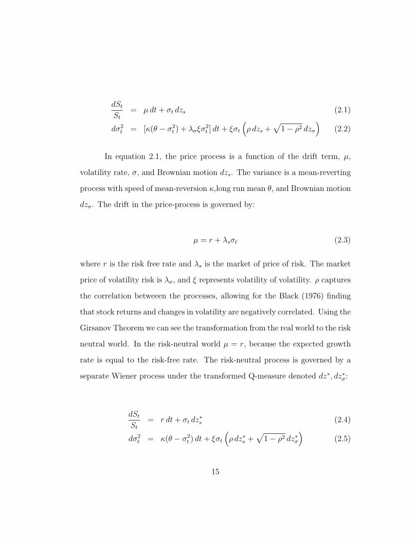
In equation 2.1, the price process is a function of the drift term, µ,
volatility rate, σ, and Brownian motion dzs. The variance is a mean-reverting
process with speed of mean-reversion κ,long run mean θ, and Brownian motion
dzσ. The drift in the price-process is governed by:
µ = r + λsσt (2.3)
where r is the risk free rate and λs is the market of price of risk. The market
price of volatility risk is λσ, and ξ represents volatility of volatility. ρ captures
the correlation betweeen the processes, allowing for the Black (1976) finding
that stock returns and changes in volatility are negatively correlated. Using the
Girsanov Theorem we can see the transformation from the real world to the risk
neutral world. In the risk-neutral world µ = r, because the expected growth
rate is equal to the risk-free rate. The risk-neutral process is governed by a
separate Wiener process under the transformed Q-measure denoted dz∗, dz∗σ:
dSt
St
= r dt+ σt dz∗s (2.4)
dσ2t = κ(θ − σ2
t ) dt+ ξσt
(ρ dz∗s +
√1− ρ2 dz∗σ
)(2.5)
15
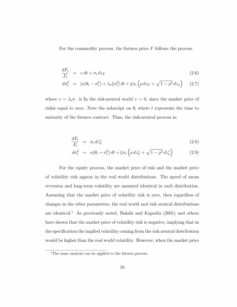
For the commodity process, the futures price F follows the process
dFt
Ft
= υ dt+ σt dzF (2.6)
dσ2t = [κ(θt − σ2
t ) + λσξσ2t ] dt+ ξσt
(ρ dzF +
√1− ρ2 dzσ
)(2.7)
where υ = λsσ. is In the risk-neutral world υ = 0, since the market price of
riskis equal to zero. Note the subscript on θt where t represents the time to
maturity of the futures contract. Thus, the risk-neutral process is:
dFt
Ft
= σt dz∗F (2.8)
dσ2t = κ(θt − σ2
t ) dt+ ξσt
(ρ dz∗F +
√1− ρ2 dz∗σ
)(2.9)
For the equity process, the market price of risk and the market price
of volatility risk appear in the real world distributions. The speed of mean
reversion and long-term volatility are assumed identical in each distribution.
Assuming that the market price of volatility risk is zero, then regardless of
changes in the other parameters, the real world and risk neutral distributions
are identical.1 As previously noted, Bakshi and Kapadia (2001) and others
have shown that the market price of volatility risk is negative, implying that in
the specification the implied volatility coming from the risk neutral distribution
would be higher than the real world volatility. However, when the market price
1The same analysis can be applied to the futures process.
16
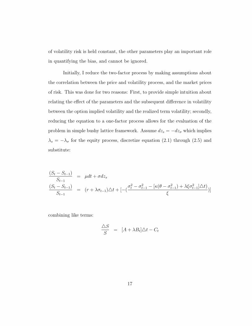
of volatility risk is held constant, the other parameters play an important role
in quantifying the bias, and cannot be ignored.
Initially, I reduce the two-factor process by making assumptions about
the correlation between the price and volatility process, and the market prices
of risk. This was done for two reasons: First, to provide simple intuition about
relating the effect of the parameters and the subsequent difference in volatility
between the option implied volatility and the realized term volatility; secondly,
reducing the equation to a one-factor process allows for the evaluation of the
problem in simple bushy lattice framework. Assume dzs = −dzσ which implies
λs = −λσ for the equity process, discretize equation (2.1) through (2.5) and
substitute:
(St − St−1)
St−1
= µdt+ σdzs
(St − St−1)
St−1
= (r + λσt−1)4t+ [−(σ2
t − σ2t−1 − [κ(θ − σ2
t−1) + λξσ2t−1]4t)
ξ)]
combining like terms:
4SS
= [A+ λBt]4t− Ct
17

with
A = r +κθ
ξ
Bt = (σt−1 − σ2t−1)
Ct =σ2
t − σ2t−1(1− κ)
ξ
For the risk neutral process, the equations combine in a similar fashion to
4SS
= A4t − Ct, since λ = 0. Within the reduced factor process it becomes
easy to interpret the effect of an increase in λ on the change in price, and
subsequently, the volatility process. If λ is equal to zero, then we should
expect exactly the same price movements in the risk neutral process and the
real world process. However, when there is positive market price of risk, as is
the case for equities, the two processes should diverge. To evaluate the effect of
λ, I use the bushy lattice framework since the volatility is not constant. Solving
for the bushy lattice, it is easy to see the evolution of the price tree for the two
processes.2 I combine the risk neutral process with the real world process and
am left with 4S∗
S∗= 4S
S− λB4t. Since λ is positive, and σ must always be
positive, the change in the real world price must be greater than that of the
risk neutral process. From the assumption of perfect negative correlation, it
should then hold that the volatility change is more volatile for the risk neutral
process. This is easily shown by substituting equations (2.2) into (2.3), and
2Please refer to appendix for discussion on the technique used for the bushy lattice.
18
(2.4) into (2.5). The proof is shown in the Appendix. Given that the market
price of risk is positive for equities, and that dzs, dzσ are perfectly negatively
correlated, there is a resulting negative effect on the volatility change due to a
negative market price of volatility risk. This results in a less volatile process for
the objective distribution. For commodities, the same intuition applies except
that there is a negative market price of risk and perfect positive correlation
between the processes.3
If there exists a negative market price of volatiltiy risk, then result-
ing risk-neutral and real-world volatilties should demonstrate the properties
shown above for both equites and commodities. Hereto, Black-Scholes (Black)
implied volatility should be greater than realized term volatility for equities
(commodities). This can be tested by regressing Black-Scholes implied volatil-
ity (BSIV) on realized-term volatility and showing that BSIV is an upward-bias
predictor of realized-term volatiltiy.
2.3 Estimation of the Bias in BSIV/BIV
2.3.1 Data
To test the bias in BSIV/BIV, and later for the data generating process,
I use the S&P 500 and S&P 100 Index for the equity/index process and ten
years of gas futures contracts that expire in each month of the year. I have
3The assumption of perfect correlation will be relaxed in the following chapter for bothsimulation of the model and estimation of the data. For the simulation, the bushy-latticetechnique will be replaced with a quasi-Monte Carlo procedure.
19
collected daily price and annualized daily-implied volatility from October 1994
until July 2001 for the S&P 500 and from January 1st 1986 to August 26th
2002 for the S&P 100. For the gas contracts, I have futures and options prices
for all the options contracts starting with a contract that expired January 1995
and finishing with a contract that expires December 2005. I will focus on all
the contracts and will control for seasonality issues. The option and price data
has come from Bloomberg. Bloomberg constructs an implied volatility based
on a weighted average of closing prices of call and put options with time to
maturity as close to 22 days. For estimating bias I look only at ATM forward
call and put options. I will address the potential measurement error issues
shortly. The gas contracts implied volatility comes from the actual contracts,
and thus the term-structure of volatility (TSOV) must be accounted for. The
implied volatility for the S&P 100 was collected from the VIX index.4 The
daily risk free rate comes from the Federal Reserve for the 1-month T-Bill.
The frequency of the data is daily. Currently there are 1959 days for the S&P
500, 4183 days for the S&P 100, and 5067 combined days for the gas futures
contracts. Table 1 provides the descriptive statistics for the both the implied
volatility and realized term volatility5 for the S&P 100 and the S&P500. The
sample clearly indicates that implied volatility has been higher than realized
volatility for both indices as well as the pre- and post- October 1987 crash.
4The implied volatility from the VIX index was caluclated using the old methodology.The method for calculating BSIV was changed in 2003.
5Please refer to equations 3.9-3.10 for reference on the calculation of realized term volatil-ity.
20
Figure 2 shows the time series of implied volatility for both the S&P 100
and S&P 500 with daily price movements of 3% and 5%. This is shown to
highlight how infrequently the index had moved in these amounts on a daily
basis over this period. In addition, tables 3-4 document how often gas prices
have jumped in daily movements of over 5% and 10%. Table 2 has descriptive
statistics of daily returns for the natural gas futures contracts. What is evident
is the degree of volatility present in gas prices, and to what extent that these
“jumps” are clustered in certain years and monthly contracts. Controlling for
these effects will be crucial in the estimation procedure. Figure 3 shows the
daily implied volatility level for each of the gas contracts for January and July
in years 1995 and 2001, which gives the best description of the effect of the
TSOV.
2.3.1.1 Measurement Error
As Hentschel (2002) points out, the potential measurement error in
implied volatility can range from insignificant to potentially disastrous. The
problem in inferring implied volatilities from the Black-Scholes formula is that
small pricing errors in the stock price and call price can lead to large distor-
tions in the inverted volatility. The problem is relatively insignificant for the
ATM options, especially for index options, but becomes exponentially worse
for deep ITM and OTM options.6 However, since for this particular estimation
I only look at a constructed estimates of implied volatility for all contacts, the
6Refer to table 2a,b in Hentschel (2002) for example.
21
concern with measurement error is minimized. The difference between VIX
and the GLS correction in Hentschel (2002) is insignificant, and since the
Bloomberg HIVG estimate is constructed in a similar manner, I am confident
in the precision of the results.
2.3.2 Estimating the bias
2.3.2.1 Equity Bias
The hypothesis that Black-Scholes is an efficient and unbiased predictor
of realized term volatility is assessed by estimating a regression of the form
ht = α0 + αiit + εt (2.10)
where ht denotes the realized term volatility for period t and it denotes the
implied volatility from the Black-Scholes closed form solution at the beginning
of period t.7 For BSIV to be unbiased, it must be the case that α0 = 0 and
αi = 1; for efficiency the residuals should be white noise and uncorrelated
with the independent variables. As Christiansen and Prabhala (1998) note,
there could be an errors-in-variables (EIV) problem with using BSIV, and use
prior-month BSIV as an instrument. This they feel helps resolve the issue of
7ht is Christensen and Prabhala definition of realized term volatility as given in equation2 of their paper and equations 3.9 and 3.10 in this chapter. Additional specification add inpast realized term volatility such that ht = α0 + αiit + αhht−1 + εt. This was run despitethe multi-collinearity problem. The correlation between it and ht−1 for the S&P 100 wasaround .8. For the S&P 500 the correlation was close to .4. This is independent of level orlog-level specification.
22
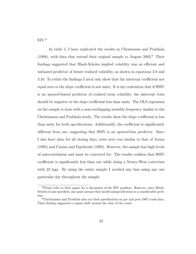
EIV.8
In table 5, I have replicated the results in Christensen and Prabhala
(1998), with data that extend their original sample to August 2002.9 Their
findings suggested that Black-Scholes implied volatility was an efficient and
unbiased predictor of future realized volatility, as shown in equations 3.9 and
3.10. To refute the findings I need only show that the intercept coefficient not
equal zero or the slope coefficient is not unity. It is my contention that if BSIV
is an upward-biased predictor of realized term volatility, the intercept term
should be negative or the slope coefficient less than unity. The OLS regression
on the sample is done with a non-overlapping monthly frequency similar to the
Christiansen and Prabhala study. The results show the slope coefficient is less
than unity for both specifications. Additionally, the coefficient is significantly
different from one, suggesting that BSIV is an upward-bias predictor. Since
I also have data for all closing days, tests were run similar to that of Jorion
(1995) and Canina and Figelweski (1993). However, the sample has high levels
of autocorrelation and must be corrected for. The results confirm that BSIV
coefficient is significantly less than one while doing a Newey-West correction
with 22 lags. By using the entire sample I avoided any bias using any one
particular day throughout the sample.
8Please refer to their paper for a discussion of the EIV problem. However, since Black-Scholes is mis-specified, one must assume that model-misspecification is a considerable prob-lem.
9Christiansen and Prabhala also ran their specification on pre and post 1987 crash data.Their finding suggested a regime shift around the time of the crash.
23
This particular specification was done on levels of volatility versus log-
levels. In this analysis I will examine both the levels and log-levels of volatil-
ity even though log-levels seem to be more appropriate. The Christiansen
and Prabhala (1998) study also notes that implied volatility may incorporate
measurement error, and uses the prior month’s implied volatility as well as
prior month realized term volatility as an instrument.10 The results on levels
show the slope term is significantly different for one. As for the results on
the log-levels, the intercept term is negative and significantly different from
zero, suggesting upward-bias in BSIV. I find these results give foundation for
relating this bias to the underlying parameters that drive stock prices and
volatility.
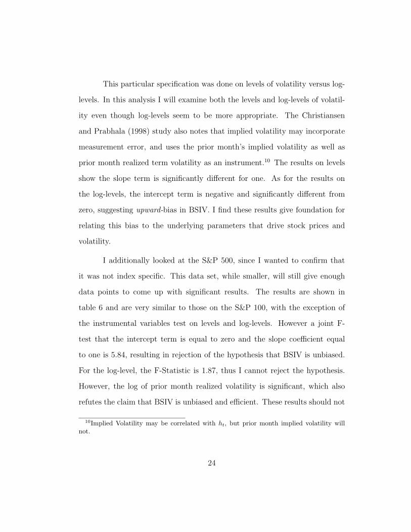
I additionally looked at the S&P 500, since I wanted to confirm that
it was not index specific. This data set, while smaller, will still give enough
data points to come up with significant results. The results are shown in
table 6 and are very similar to those on the S&P 100, with the exception of
the instrumental variables test on levels and log-levels. However a joint F-
test that the intercept term is equal to zero and the slope coefficient equal
to one is 5.84, resulting in rejection of the hypothesis that BSIV is unbiased.
For the log-level, the F-Statistic is 1.87, thus I cannot reject the hypothesis.
However, the log of prior month realized volatility is significant, which also
refutes the claim that BSIV is unbiased and efficient. These results should not
10Implied Volatility may be correlated with ht, but prior month implied volatility willnot.
24

be surprising given that we know that the data cannot be described by a pure
Black-Scholes model. If there is a negative market price of volatility risk, we
should expect that Black-Scholes implied volatility is an upward-bias predictor
of future realized volatility.
When adding prior month realized volatility to the specification, I still
find implied volatility as the best predictor for future realized volatility.11 The
estimates based on prior realized volatility tend to be insignificant at either
the statistic or economic level. This is an important result. Regardless of the
bias nature in implied volatility, it still appears to be the strongest forecast of
future volatility in the market. By providing these reliable estimates on the
bias in implied volatility I provide better forecasts of future market movements
with BSIV.
Interpreting the instrumental variables test for BSIV levels of 15%,
20%, and 30% on the S&P 100 translated into realized term volatility levels of
10.41%, 13.88%, and 20.82%. For the S&P 500 these BSIV levels translate into
9.36%, 14.08%, and 23.52% for realized term volatility. It is my contention
that as the volatility in the equity markets rises, the degree to which BSIV is
an upward-bias forecast of future volatility also increases.
11Canina and Figelweski (1993) suggest that prior month realized volatility is the efficientpredictor for future realized volatility
25
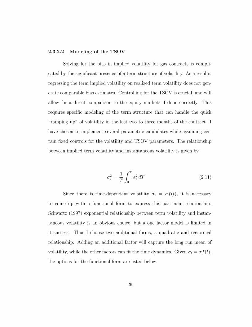
2.3.2.2 Modeling of the TSOV
Solving for the bias in implied volatility for gas contracts is compli-
cated by the significant presence of a term structure of volatility. As a results,
regressing the term implied volatility on realized term volatility does not gen-
erate comparable bias estimates. Controlling for the TSOV is crucial, and will
allow for a direct comparison to the equity markets if done correctly. This
requires specific modeling of the term structure that can handle the quick
“ramping up” of volatility in the last two to three months of the contract. I
have chosen to implement several parametric candidates while assuming cer-
tain fixed controls for the volatility and TSOV parameters. The relationship
between implied term volatility and instantaneous volatility is given by
σ2T =
1
T
∫ T
0
σ2t dT (2.11)
Since there is time-dependent volatility σt = σf(t), it is necessary
to come up with a functional form to express this particular relationship.
Schwartz (1997) exponential relationship between term volatility and instan-
taneous volatility is an obvious choice, but a one factor model is limited in
it success. Thus I choose two additional forms, a quadratic and reciprocal
relationship. Adding an additional factor will capture the long run mean of
volatility, while the other factors can fit the time dynamics. Given σt = σf(t),
the options for the functional form are listed below.
26

Exponential f(t) = e−α t
Reciprocal f(t) = α+ βt
Quadratic f(t) = α+ β t+ γ t2
where t is time to maturity and α, β, and γ are TSOV parameters to
be estimated.
With daily observations for each month over a ten year span, it is neces-
sary to make certain assumptions to solve for the correct specification. I have
chosen to vary the volatility for each contract and have a fixed term structure
parameter by months to allow for yearly variations in volatility and monthly
differences for term structure controls. However, I restrict the volatility to be
constant for each day within each contract and allow the TSOV parameter
to capture the increase in volatility towards maturity. It is possible to have
chosen to let volatility vary each day of the contract while holding the volatil-
ity across contracts constant. While this will obviously improve model fit, it
diminishes the impact of the TSOV parameter, and will not reflect the true
relationship between the instantaneous volatility and 30 day estimate. The
objective function is stated below
min(α,β,γ,σt)
N∑i=1
T∑t=τ
[σ2
it −σ2
i
T − t
∫ T
t
f 2(t) dt
]2
(2.12)
where σit is implied volatility on date t and year i. σi is a year i constant
to be estimated. Equation 2.12 is minimized and in-sample fit is analyzed to
assess which model fits best. The addition of the long run factor helps with
27

overall model fit, but the results are highly dependent on the given contract
month. The exponential function form performs well relative to the others
with either fitting the close-to-maturity or far-from-maturity dates depending
on the initial condition given. The quadratic tends force the curvature to fit
the close-to-maturity dates by implying negative volatilities for the 3-7 months
to maturity period. The reciprocal fits best in certain months because it allows
for the increasing convexity close-to-maturity without sacrificing earlier dates.
Figure 4 and 5 best demonstrates this.
I test for model misspecification of the TSOV by using 5-day before,
1-day before and 5-day after volatilities for each model on each day for each
contract. These tests are typical for model misspecification as discussed in
Arimya (1980) and have been used in tests of various option models as in Bak-
shi, Cao and Chen (1997). The typical argument is that with more structural
parameters it becomes easier to fit a given model, but can cause overfitting
which will result in poor out-of-sample performance. Again minimization was
done on the objective function as given before and tests each monthly con-
tract. The results are presented in table 7 along with the in-sample results.
The results suggest that either Schwartz (1997) exponential model or the re-
ciprocal functions are the best candidates for the TSOV for gas contracts.
For each month the apparent in-sample candidate model also performs best in
the out-of-sample tests. A closer look at the January results show the perfor-
mance of the exponential model is best in all three out-of-sample tests with
the reciprocal function showing large performance improvements when using
28

5-day behind volatilities. This is suggestive of a pontential problem either
with the final couple of days of volatility in a given contract or the reciprocal
model itself. One fault in the estimation relies on the taking the log of in-
finity, which requires an approximation, and this approximation can result in
large errors when maturity of a given contract approaches. This seems to be
apparent given the results for January, where there exists a large TSOV and
poor reciprocal fit, and the results for May, which are the opposite.12
I extend the analysis by breaking up each test into individual years for a
given monthly contract and testing each model on those years. The concern is
that the results may hinge on the poor fit of one particular year thus distorting
the overall fit through the minimization of equation 2.12. For example, let year
1995 have no significant TSOV while other years have significant slopes. This
can result in a greater penalty for a given model, say the exponential, for
year 1995, while that same model fits the other years better than the other
potential parametric candidates. It may then be better to examine the years
one by one versus collectively since each year has a unique TSOV associated
with it. Below I break up the January estimation into individual years, and
examine the individual RMSE to asses the model fit. Initially it appears that
the exponential fit does best for the overall period, given the in and out-of-
sample fits. The table below suggests that the other models do better for
certain years. There is no apparent trend as the reciprocal model performs
12These particular months were choosen to shown the disparity between months that haslarge TSOV effects and months that did not. Likewise, December and April could have beenselected for this particular comparision.
29
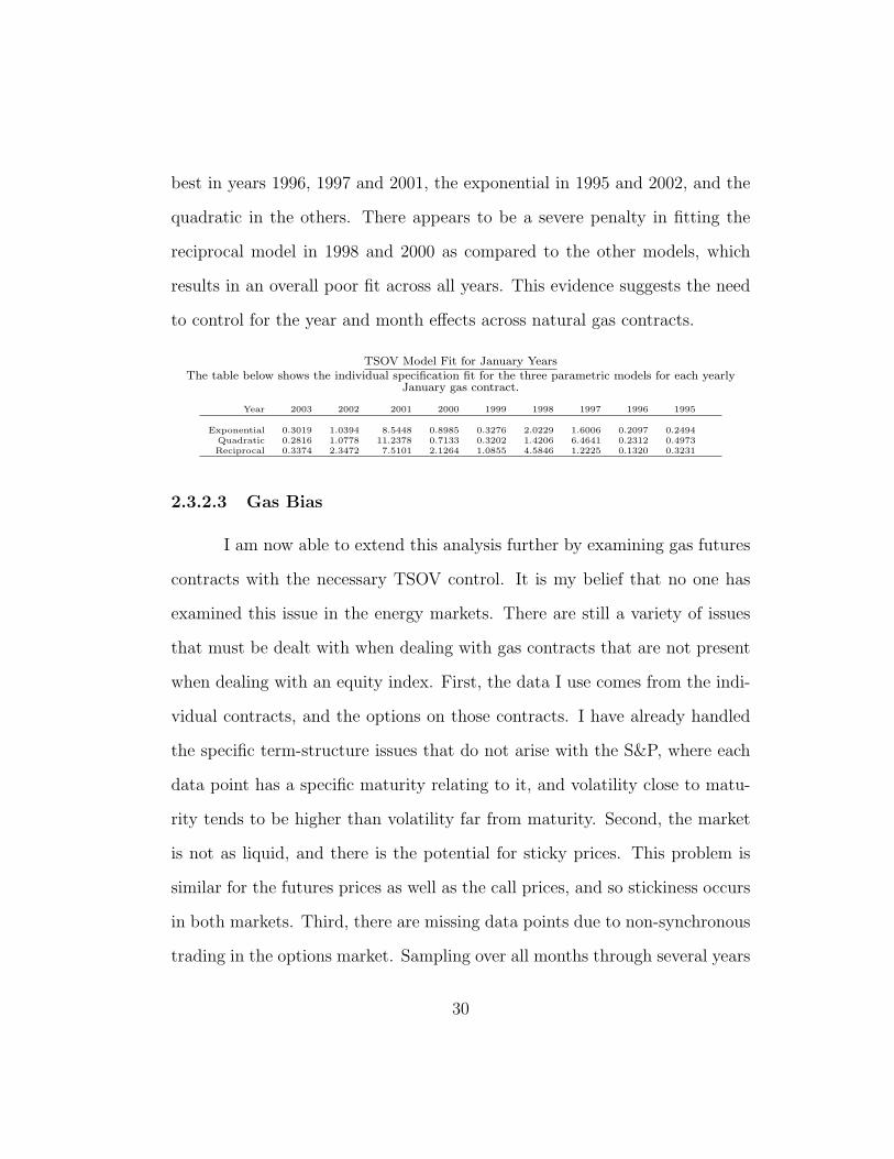
best in years 1996, 1997 and 2001, the exponential in 1995 and 2002, and the
quadratic in the others. There appears to be a severe penalty in fitting the
reciprocal model in 1998 and 2000 as compared to the other models, which
results in an overall poor fit across all years. This evidence suggests the need
to control for the year and month effects across natural gas contracts.
TSOV Model Fit for January YearsThe table below shows the individual specification fit for the three parametric models for each yearly
January gas contract.
Year 2003 2002 2001 2000 1999 1998 1997 1996 1995
Exponential 0.3019 1.0394 8.5448 0.8985 0.3276 2.0229 1.6006 0.2097 0.2494Quadratic 0.2816 1.0778 11.2378 0.7133 0.3202 1.4206 6.4641 0.2312 0.4973Reciprocal 0.3374 2.3472 7.5101 2.1264 1.0855 4.5846 1.2225 0.1320 0.3231
2.3.2.3 Gas Bias
I am now able to extend this analysis further by examining gas futures
contracts with the necessary TSOV control. It is my belief that no one has
examined this issue in the energy markets. There are still a variety of issues
that must be dealt with when dealing with gas contracts that are not present
when dealing with an equity index. First, the data I use comes from the indi-
vidual contracts, and the options on those contracts. I have already handled
the specific term-structure issues that do not arise with the S&P, where each
data point has a specific maturity relating to it, and volatility close to matu-
rity tends to be higher than volatility far from maturity. Second, the market
is not as liquid, and there is the potential for sticky prices. This problem is
similar for the futures prices as well as the call prices, and so stickiness occurs
in both markets. Third, there are missing data points due to non-synchronous
trading in the options market. Sampling over all months through several years
30
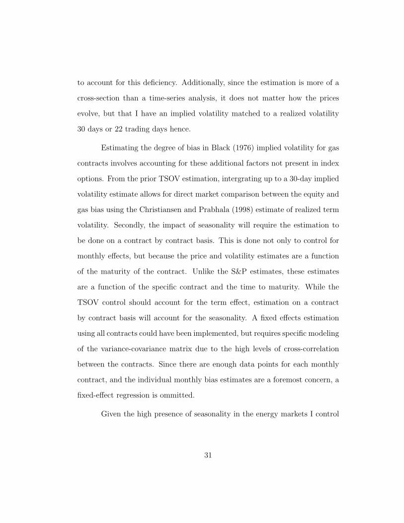
to account for this deficiency. Additionally, since the estimation is more of a
cross-section than a time-series analysis, it does not matter how the prices
evolve, but that I have an implied volatility matched to a realized volatility
30 days or 22 trading days hence.
Estimating the degree of bias in Black (1976) implied volatility for gas
contracts involves accounting for these additional factors not present in index
options. From the prior TSOV estimation, intergrating up to a 30-day implied
volatility estimate allows for direct market comparison between the equity and
gas bias using the Christiansen and Prabhala (1998) estimate of realized term
volatility. Secondly, the impact of seasonality will require the estimation to
be done on a contract by contract basis. This is done not only to control for
monthly effects, but because the price and volatility estimates are a function
of the maturity of the contract. Unlike the S&P estimates, these estimates
are a function of the specific contract and the time to maturity. While the
TSOV control should account for the term effect, estimation on a contract
by contract basis will account for the seasonality. A fixed effects estimation
using all contracts could have been implemented, but requires specific modeling
of the variance-covariance matrix due to the high levels of cross-correlation
between the contracts. Since there are enough data points for each monthly
contract, and the individual monthly bias estimates are a foremost concern, a
fixed-effect regression is ommitted.
Given the high presence of seasonality in the energy markets I control
31

for each month of expiration for the futures contracts.13 This is accomplished
by running separate regressions for each month and accounting for the year
effects through the TSOV corrections. The results are shown in table 8. I
correct the heteroskedacity through a white correction as well as running a
weighted-least-squares using implied volatility as the weight.14 Regressions
were run using only the starting day in each month,15 and then using the full
sample with Newey-West corrected errors done at 22 day lags. This was done
for two reasons. First, the full sample cannot be used due to the high pres-
ence of auto-correlation at the daily level, and second, to have results that
were comparable to those for the equity regressions ran earlier. The findings
are quite different to those reported for the equity index regression, however,
result in the same conclusion that BIV would have to be upward-bias. What
is immediately obvious is that bias decreases as implied volatility increases.
This is not surprising since we observe the highest levels of volatility close to
maturity for these contracts. Typically, realized volatility increases as matu-
rity approaches and can even exceed implied volatility.16 However, even with
a slope coefficient greater than unity, the intercept coefficients are negative,
and significantly different from zero. For the January, July, November, and
December months, the intercept term is close to 1. A t-test on the slope coef-
13Summer and winter months tend to have more demand due to the excessive heat/cold.It is during these months that most price spikes occur.
14results suppressed.15I also ran this specification using the last day of every month, and the middle of each
month, with the results coming up similar to those reported16this can also be a function of how realized volatility is calculated. As maturity ap-
proaches, statistical variance increases.
32
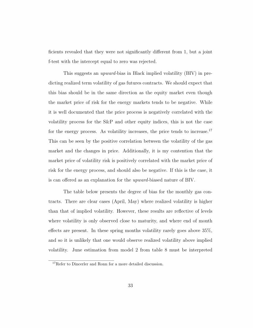
ficients revealed that they were not significantly different from 1, but a joint
f-test with the intercept equal to zero was rejected.
This suggests an upward-bias in Black implied volatility (BIV) in pre-
dicting realized term volatility of gas futures contracts. We should expect that
this bias should be in the same direction as the equity market even though
the market price of risk for the energy markets tends to be negative. While
it is well documented that the price process is negatively correlated with the
volatility process for the S&P and other equity indices, this is not the case
for the energy process. As volatility increases, the price tends to increase.17
This can be seen by the positive correlation between the volatility of the gas
market and the changes in price. Additionally, it is my contention that the
market price of volatility risk is positively correlated with the market price of
risk for the energy process, and should also be negative. If this is the case, it
is can offered as an explanation for the upward-biased nature of BIV.
The table below presents the degree of bias for the monthly gas con-
tracts. There are clear cases (April, May) where realized volatility is higher
than that of implied volatility. However, these results are reflective of levels
where volatility is only observed close to maturity, and where end of month
effects are present. In these spring months volatility rarely goes above 35%,
and so it is unlikely that one would observe realized volatility above implied
volatility. June estimation from model 2 from table 8 must be interpreted
17Refer to Dincerler and Ronn for a more detailed discussion.
33

with caution because of the impact that prior month realized volatility had on
the estimate. However, the R2 from model 1 to model 2 only added 10% of
explanatory power and thus model 1 estimates may be more appropriate. By
comparison, at the 20% volatility level, the gas markets tend to exhibit greater
BSIV/BIV bias versus the equity markets, especially for the winter months.
Given that the energy markets are more volatile, and that we observe greater
BIV/BIV bias, could this tell us something about the proportional premium
placed on volatility in these markets? Should we expect that the market price
of volatility risk in the gas markets will be higher in absolute terms? A major
goal of this work is to determine this out by relating the bias to the parame-
ters that govern the volatility process. I have demonstrated the upward-bias
in BIV. This allows for testing the feasibility of various option pricing models
as well as prior estimated parameters from these models. If a model can attain
this level of bias, it further indicates the appropriateness of the specification.
Bias in BIVThe table below show the bias in BIV relative to realized term volatility. For a given level of BIV the table
shows for each month the difference between BIV and realized term volatility. Model 1 is the initialspecification given equation 2.12. Model 2 incorporates prior realized term volatility.
Model 1 Model 2
20.00% 30.00% 40.00% 20.00% 30.00% 40.00%
Jan 9.38% 7.77% 6.16% 11.90% 12.35% 12.80%Feb 11.02% 8.23% 5.44% 14.36% 15.84% 17.32%Mar 11.16% 7.84% 4.52% 11.36% 7.24% 3.12%Apr 9.80% 4.65% -0.50% 10.10% 5.05% 0.00%May 6.46% 2.29% -1.88% 6.02% 2.33% -1.36%Jun 0.42% 2.73% 5.04% 9.74% 15.96% 22.18%Jul 5.56% 4.29% 3.02% 6.96% 7.09% 7.22%
Aug 6.32% 3.73% 1.14% 4.86% 1.14% -2.58%Sep 6.40% 4.00% 1.60% 7.78% 4.02% 0.26%Oct 7.30% 4.35% 1.40% 5.80% 2.20% -1.40%Nov 6.66% 5.64% 4.62% 5.68% 3.42% 1.16%Dec 9.40% 8.60% 7.80% 12.48% 13.32% 14.16%
34
2.4 Conclusion
The implications of the findings in this section confirm two important
prior results; first, that the Black-Scholes model is misspecified, and second,
BSIV is still the efficient predictor of future realized volatiltiy. Additonally, the
results for the equities markets transfer directly to the commodities markets,
specifically for natural gas futures and the Black model. Controlling for the
term structure of volatility allows for a direct comparison between the equities
and the commodities markets, and the results reveal that both BSIV and BIV
are upward-bias predictors of σRTV .
This is highly relevant since the degree of the bias can be related to the
underlying data generating process that governs stock and futures prices. An
upward-bias in BSIV/BIV is suggestive of a negative market price of volatility
risk. The intent of the next section is to use these results and relate them
to various instantaneous structural models that incorporate both stochastic
volatility and jumps. Through Monte Carlo simulation and mean-reversion
estimation, the market price of volatiltiy risk can be extracted using the esti-
mated degree of bias found in tables 5, 6, and 8.
35
Chapter 3
Monte Carlo Simulation and Estimation of the
Market Price of Volatility Risk
3.1 Introduction
Using the knowledge attained through the upward- bias relationship be-
tween BSIV/BIV and realized-term volatility, I will calibrate the underlying
data generating process from both the risk-neutral and real-world processes
to the degree of bias using the sensitivity of the instantaneous structural pa-
rameters. The intent here is to demonstrate that the market price of volatility
risk, λσ, is negative and significant. The first will be accomplished through
Monte Carlo simulation. The second will be demonstrated by the simulations
incorporating many parameterizations, and showing that a large negative λσ is
necessary, and independent of model specification, to demonstrate the degree
of upward-bias shown in the previous chapter. Once this claim has been estab-
lished, the estimation of the market price of volatility risk will be conducted
using a stochastic volatility mean reverting framework. Using a time-series
of implied volatilities from short-term at-the-money (ATM) options and con-
structed realized-term volatilties, the market price of volatility risk can be
estimated via calibration.
36
3.2 Monte Carlo Simulation
I adopt Monte Carlo simulation to test for the sensitivity of the bias
in BSIV to realized term volatility in the underlying parameters of the model.
The stochastic volatility simulation is executed using equations (2.1)-(2.5) for
the equity process, and equations (2.6)-(2.9) for the commodity process. For
completeness, I present the real-world and risk-neutral price and volatility
processes below:1
Real-World Process:
dSt
St
= µ dt+ σt dzs (3.1)
dσ2t = [κ(θ − σ2
t ) + λσξσ2t ] dt+ ξσt
(ρ dzs +
√1− ρ2 dzσ
)(3.2)
Risk-Neutral Process:
dSt
St
= r dt+ σt dz∗s (3.3)
dσ2t = κ(θ − σ2
t ) dt+ ξσt
(ρ dz∗s +
√1− ρ2 dz∗σ
)(3.4)
where r is the risk free rate and λs is the market of price of risk. The market
price of volatility risk is λσ, and ξ represents volatility of volatility. κ is the
speed of mean-reversion, θ is the long run mean, and rho captures the corre-
lation between the price and volatility processes. dzs and dzσ are geometric
Brownian motions. dz∗s and dz∗σ are Brownian motions transformed under the
risk-neutral measure Q.
1For the futures processes, refer to the prior chapter.
37
Two variance reduction control techniques were implemented to help
reduce the standard error of the estimate and improve the efficiency of the
results.2 For each sample path, random shocks are drawn from N ∼ (0,√4t)
at 4t intervals over the life of the option. So with a 1-month to expiration
option, 22 random shocks are drawn for the price process for 22 business days.
This procedure is replicated for the volatility process and is governed by a
separate Brownian motion. Since the concern is with both the risk-neutral
and real-world processes, a total of four random draws are needed for the
evolution of one day. The option value for a call and put are then calculated
as,
Cnt = E∗t [e−rt max(SnT −K, 0)] (3.5)
Pnt = E∗t [e−rt max(−SnT +K, 0)] (3.6)
under the risk neutral measure, where n represents the particular path.
This process is repeated for 1,000,000 runs. This is slightly excessive, but, it
was important to reach an efficient estimator for the call value since inferring
the correct volatility relies on precise estimates of fractions of a cent.3 The
final call and put values are then:
2I have used the antithetic variable and control variate techniques using Black-Scholesas the know analytical solution. In addition, I have run quasi monte-carlo simulations usingthe Sobol sequence to generate results, this was done to determine the number of runs toachieve efficiency.
3As pointed out by Hentschel (2002) and others, pricing and implied volatility errors canbe large when call prices are measured inaccurately.
38
Ct =1
n
n∑i=1
Cit (3.7)
P t =1
n
n∑i=1
Pit (3.8)
By finding C, P and given the starting value for the stock price, risk-
free rate, time to expiration, and strike price, Black-Scholes, or Black for
the gas process, can be inverted and the estimate for BSIV/BIV solved. It
is important to note that the time interval for sampling the random shocks
is small, otherwise it could lead to an instantaneous shock to the volatility
process resulting in a negative variance. For current purposes, the shocks are
bound so that there are zero negative variance realizations. Nevertheless, even
without the bound the variance process infrequently dips below zero.4
To solve for the realized term volatility two methods are adopted. The
first is to sample the returns of the stock/future over the remaining life of the
option.
σrtv =
√√√√1
t
t∑i=1
(ri − rt) (3.9)
where t is number of days to expiration, ri is return on day i and rt
is the average daily return over the option’s life. Additionally, this volatility
4The large ξ is, the large the changes in variance. This can be countered by a smallersampling interval.
39
is annualize to make an easy comparison with the BSIV. This estimate of
realized volatility has been used by Christiansen and Prabhala(1998). The
second measure is
σrtv =
√∑ni=1[(ln(STi
S0)− r)2]
√T
(3.10)
where the period variance is calculated versus the daily variance within
the period. To annualize the volatility the square-root of the period was taken
versus the sampling interval. On average these two estimates should be equal.
While not reported, the bias of BSIV to either estimate of relative term volatil-
ity is not significantly different from one another, and thus only the second
estimate is reported. Calculating mean return, r, requires the transformation
from normal to log-normal.5 This requires knowledge of σ, which is unknown
prior to finding r. This is accomplished by transforming the starting normal
mean, and calculating σ2 from this initial estimate of r. From this first esti-
mate of σ2 the initial mean is then adjusted to a log-normal estimate. The
process to find σ2 with this transformed estimate of r is repeated until con-
vergence is achieved for both values, such that the σ2 is exactly the same for
the standard deviation and the log-normal adjustment for r.6
5The mean return is adjusted from µ to µ− σ2
2 .6No iteration required more than 4 loops to achieve convergence.
40
3.2.1 Stochastic Volatility Simulation
3.2.1.1 Perfect and Zero Correlation Cases
The first tests run were base cases using zero and perfect (negative for
equities) correlation. By examining the extremes in correlation it is possible
to separate out the effect of correlation and the market price of risk on the bias
in BSIV/BIV. In the zero correlation case there should be a limited skew and
minimal bias since there is no market price of volatility risk. In the perfect
negative correlation case, the positive market price of risk is transfered into a
negative market price of volatility risk in the stochastic volatility process. As
a result a greater bias in BSIV/BIV is observed as well as a difference in the
degree of bias between the ITM, ATM, and OTM options. Table 9 shows the
results .
Note the familiar skew patterns for equities and commodities when
there is perfect correlation. This is a result of the correlation and the transfer
of the market price of risk to the market price of volatility risk. When there is
no correlation there appears to be no skew and insignificant bias. The negative
bias for the OTM calls initially seemed counter intuitive given what is known
about the relationship between implied volatility and realized volatility. How-
ever, this is not surprising given the presence of perfect negative correlation.
As the stock price rises, there is an ex-ante decrease in the underlying volatil-
ity. This decrease results in lower call values and lower implied volatilities. In
real world term, traders are less inclined to extract a premium for the OTM
calls since their downside position has improved ex-ante, and can offer the
41
buyer of the option a lower price/volatility. Since the realized term volatility
is constant across strike prices, this results in a negative relationship between
the implied volatility and realized term volatility for the OTM calls and ITM
puts.
3.2.1.2 Equity
The results for the bias in BSIV for the stochastic volatility equity
process model are shown in table 11. I have separated the results into bins of
volatility levels and time to maturity. The results for the low instantaneous
volatility levels (15%), medium levels (20%), and high levels (30%), are in
Panel A, Panel B (supressed for space), and Panel C respectively. For time to
maturity I have simulated results for a 1 month,12
year, and 1 year maturing
option. Within each bin, simulations are done across moneyness, market price
of volatility risk (λσ), and ξ. Reported are only the strike/spot ratio of .9, 1,
and 1.1, λσ of 0, -.5, ξ and -2, and of .3 and .7 for equity/index process.7 The
bias for call options is reported on the first line of each segment, put option
on the second.
An examination of Panel A shows that with no market price of volatility
risk, the bias in BSIV over realized term volatility goes from 2.25% to -0.26%
from a strike/spot ratio of .9 to 1.1. This bias appears to monotonically
increase the more negative the market price of volatility risk becomes. In
7these values are similar to those reported by other authors such as Bates (1996),Pan(2002), and others.
42

fact this is true regardless of the level of volatility, moneyness, or the time
to maturity for the option contract. When λσ is held fixed, and moneyness
increases, there is a decrease in the bias. This is not a surprise since the
bias is highly related to the skewed property observable in implied volatilities
on the SPX index, and can be tied to the negative correlation between the
two processes. Also it appears that the skew mutes through time, another
property that is related to the implied volatilities on the index. For all panels,
an increase in ξ tends to exacerbate the results, especially when λσ is -2 due
to the multiplicative nature of the parameters. For example, in Panel C, the
bias increased 3.77% for ITM call at λσ of -2 when ξ is increased from .3 to
.7. Increasing this parameter has the effect of making the stochastic volatility
process more volatile, and impacts the risk-neutral process more than the real-
world process. However, this seems to have an adverse impact in that when
λσ is low, the bias becomes significantly negative, and contradicts the prior
estimation and reduces model fit.8
This negative bias for the OTM calls initially seemed counter intuitive
given what is know about the relationship between implied volatility and re-
alized volatility. However, given the results seen in the perfect negative corre-
lation case, the results of negative bias at OTM calls are potentially plausible.
As the stock price prices rises, there is an expected ex-ante decrease in the un-
derlying volatility. This decrease results in lower call values and lower implied
8A stochastic volatility model(SV) without jumps has poor model fit relative to a stochas-tic volatility model with jumps(SVJ) since it requires ξ to be high to fit short-term optionsat the expense of long dated options.
43
volatilities. In real world terms, traders are less inclined to extract a premium
for the OTM calls since their downside position has improved ex-ante, and can
offer the buyer of the option a lower price. Since the realized term volatility
is constant across strike prices, this results in a negative relationship between
the implied volatility and realized term volatility for the OTM calls and ITM
puts.
As for level of volatility, this appears to have some impact on the bias,
suggesting that there is some proportional component to the level of the bias.
Relating that back to the results in tables 5-8, this reaffirms the results for a
negative intercept term and slope coefficient close to 1 as shown in S&P 100
and the gas contracts.
It has been well documented that implied volatilities on the index dis-
play a negative skew, thus for any model to be considered viable it is necessary
to adhere to those particular characteristics. In addition, the skew should be
muted through time due to discounting, mean-reversion, and ability to recover
from crashes/spikes. However, given that this particular model has no jumps,
should we expect a skew in implied volatilities at all? Even with stochastic
volatility, does including a market price of volatility risk add anything to the
model? Figure 5 shows the skew for the SV model for a given set of parame-
ters. The simulation results appear to show that stochastic volatility, negative
correlation between the processes, and market price of volatility risk matter in
creating a skew; but does this model match the empirical data?9 Pan (2000)
9Hull and White (1987) demonstrate the volatility skew through correlation between the
44
argues that a model without jumps cannot reconcile the cross-section of op-
tion prices. I have shown that it is necessary to have a very volatile process to
create a skew, but this can adversely affect the price of the options, making
ITM options expensive or OTM options cheap depending on maturity. At
this point in time the concern is with documenting a bias between BSIV and
realized term volatility with a stochastic volatility process and significant λσ,
not with model fit. Since jumps do matter, it is necessary then to examine
the impact jumps have in the process. Additionally, it appears that stochastic
volatility with a negative market price of volatility risk is not enough to ex-
plain the full extent of the bias, given the results provided earlier in tables 5-8.
At the minimum, an ATM bias appears to be around 7%, but even with high
levels of λσ and ξ, a bias of only 5% was achieved. Increasing the magnitude of
the parameter values produced more distorted results for the ITM and OTM
options for various maturities.
3.2.1.3 Commodities
The Monte Carlo simulation for the commodity process was run on
equations 2.6-2.9. Since the concern here is with the valuation of an option on
the price of a future, Black’s formula is implemented to determine the implied
volatility of the option. Similar to that for the equity process, results are
generated using similar underlying parameters. The correlation between price
and volatility process and the market price of risk are opposite of those of the
processes
45
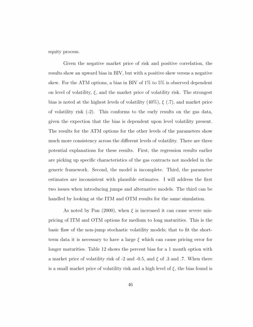
equity process.
Given the negative market price of risk and positive correlation, the
results show an upward bias in BIV, but with a positive skew versus a negative
skew. For the ATM options, a bias in BIV of 1% to 5% is observed dependent
on level of volatility, ξ, and the market price of volatility risk. The strongest
bias is noted at the highest levels of volatility (40%), ξ (.7), and market price
of volatility risk (-2). This conforms to the early results on the gas data,
given the expection that the bias is dependent upon level volatility present.
The results for the ATM options for the other levels of the parameters show
much more consistency across the different levels of volatility. There are three
potential explanations for these results. First, the regression results earlier
are picking up specific characteristics of the gas contracts not modeled in the
generic framework. Second, the model is incomplete. Third, the parameter
estimates are inconsistent with plausible estimates. I will address the first
two issues when introducing jumps and alternative models. The third can be
handled by looking at the ITM and OTM results for the same simulation.
As noted by Pan (2000), when ξ is increased it can cause severe mis-
pricing of ITM and OTM options for medium to long maturities. This is the
basic flaw of the non-jump stochastic volatility models; that to fit the short-
term data it is necessary to have a large ξ which can cause pricing error for
longer maturities. Table 12 shows the percent bias for a 1 month option with
a market price of volatility risk of -2 and -0.5, and ξ of .3 and .7. When there
is a small market price of volatility risk and a high level of ξ, the bias found is
46
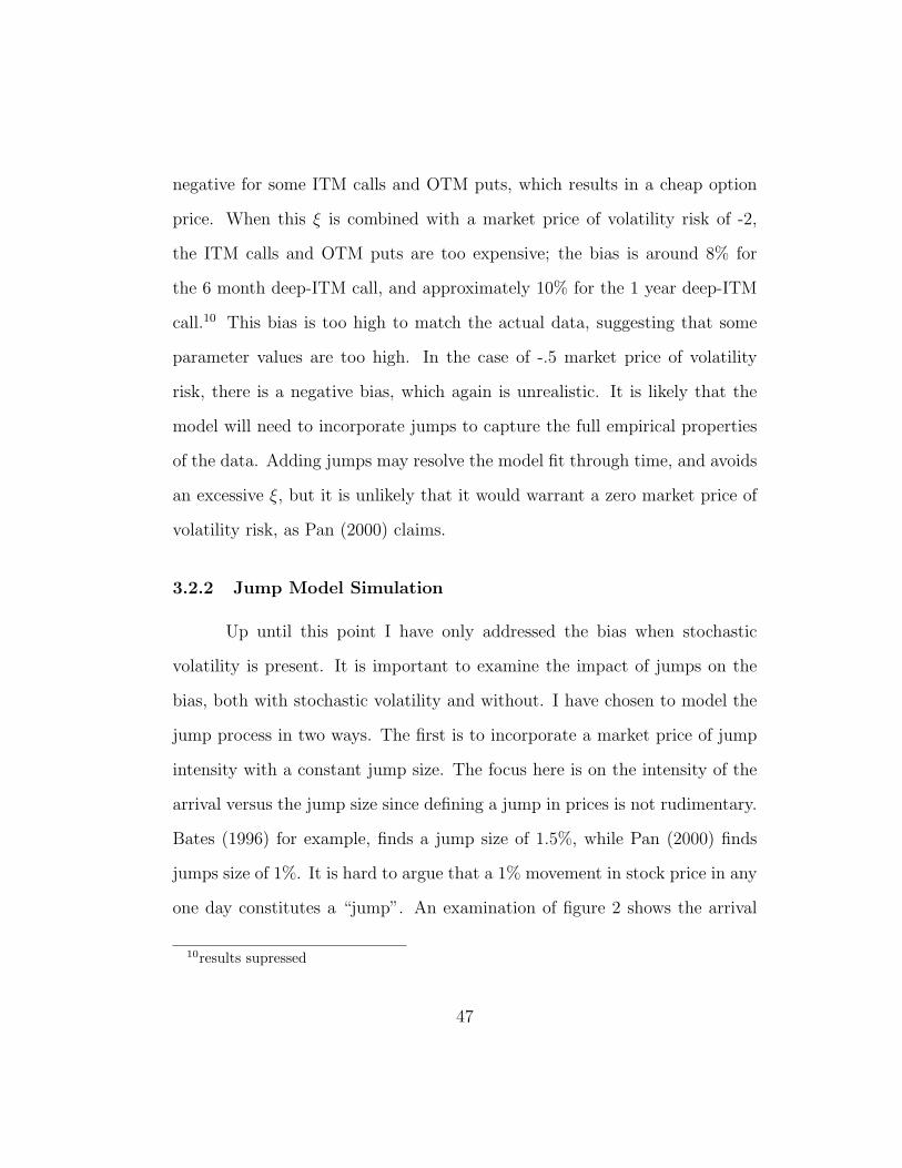
negative for some ITM calls and OTM puts, which results in a cheap option
price. When this ξ is combined with a market price of volatility risk of -2,
the ITM calls and OTM puts are too expensive; the bias is around 8% for
the 6 month deep-ITM call, and approximately 10% for the 1 year deep-ITM
call.10 This bias is too high to match the actual data, suggesting that some
parameter values are too high. In the case of -.5 market price of volatility
risk, there is a negative bias, which again is unrealistic. It is likely that the
model will need to incorporate jumps to capture the full empirical properties
of the data. Adding jumps may resolve the model fit through time, and avoids
an excessive ξ, but it is unlikely that it would warrant a zero market price of
volatility risk, as Pan (2000) claims.
3.2.2 Jump Model Simulation
Up until this point I have only addressed the bias when stochastic
volatility is present. It is important to examine the impact of jumps on the
bias, both with stochastic volatility and without. I have chosen to model the
jump process in two ways. The first is to incorporate a market price of jump
intensity with a constant jump size. The focus here is on the intensity of the
arrival versus the jump size since defining a jump in prices is not rudimentary.
Bates (1996) for example, finds a jump size of 1.5%, while Pan (2000) finds
jumps size of 1%. It is hard to argue that a 1% movement in stock price in any
one day constitutes a “jump”. An examination of figure 2 shows the arrival
10results supressed
47
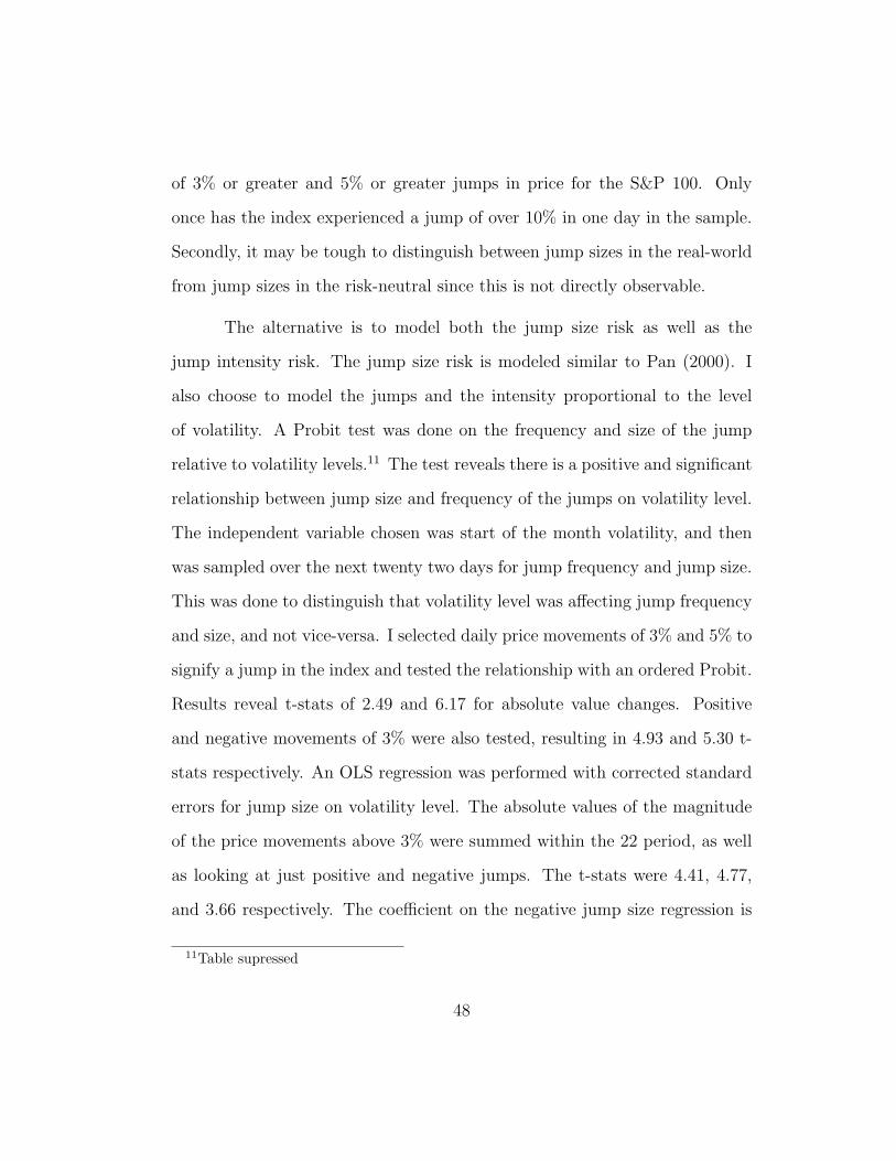
of 3% or greater and 5% or greater jumps in price for the S&P 100. Only
once has the index experienced a jump of over 10% in one day in the sample.
Secondly, it may be tough to distinguish between jump sizes in the real-world
from jump sizes in the risk-neutral since this is not directly observable.
The alternative is to model both the jump size risk as well as the
jump intensity risk. The jump size risk is modeled similar to Pan (2000). I
also choose to model the jumps and the intensity proportional to the level
of volatility. A Probit test was done on the frequency and size of the jump
relative to volatility levels.11 The test reveals there is a positive and significant
relationship between jump size and frequency of the jumps on volatility level.
The independent variable chosen was start of the month volatility, and then
was sampled over the next twenty two days for jump frequency and jump size.
This was done to distinguish that volatility level was affecting jump frequency
and size, and not vice-versa. I selected daily price movements of 3% and 5% to
signify a jump in the index and tested the relationship with an ordered Probit.
Results reveal t-stats of 2.49 and 6.17 for absolute value changes. Positive
and negative movements of 3% were also tested, resulting in 4.93 and 5.30 t-
stats respectively. An OLS regression was performed with corrected standard
errors for jump size on volatility level. The absolute values of the magnitude
of the price movements above 3% were summed within the 22 period, as well
as looking at just positive and negative jumps. The t-stats were 4.41, 4.77,
and 3.66 respectively. The coefficient on the negative jump size regression is
11Table supressed
48
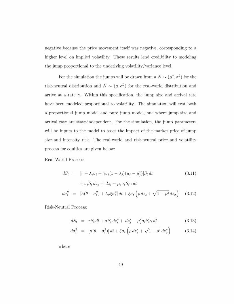
negative because the price movement itself was negative, corresponding to a
higher level on implied volatility. These results lend credibility to modeling
the jump proportional to the underlying volatility/variance level.
For the simulation the jumps will be drawn from a N ∼ (µ∗, σ2) for the
risk-neutral distribution and N ∼ (µ, σ2) for the real-world distribution and
arrive at a rate γ. Within this specification, the jump size and arrival rate
have been modeled proportional to volatility. The simulation will test both
a proportional jump model and pure jump model, one where jump size and
arrival rate are state-independent. For the simulation, the jump parameters
will be inputs to the model to asses the impact of the market price of jump
size and intensity risk. The real-world and risk-neutral price and volatility
process for equities are given below:
Real-World Process:
dSt = [r + λsσt + γσt(1− λj)(µj − µ∗j)]St dt (3.11)
+σtSt dzs + dzj − µjσtStγ dt
dσ2t = [κ(θ − σ2
t ) + λσξσ2t ] dt+ ξσt
(ρ dzs +
√1− ρ2 dzσ
)(3.12)
Risk-Neutral Process:
dSt = rSt dt+ σSt dz∗s + dz∗j − µ∗jσtStγ dt (3.13)
dσ2t = [κ(θ − σ2
t )] dt+ ξσt
(ρ dz∗s +
√1− ρ2 dz∗σ
)(3.14)
where
49

1. λs, λσ, λj, and (µj − µ∗j), are the market price of risk, market price of
volatility risk, market price of jump intensity risk, and market price of
jump size risk respectively. Jump intensity and size risk are proportional
to volatility.
2. ρ is the correlation between the price and volatility processes
3. dzj, γ, and µj are the jump process, the jump intensity (arrival rate),
and the jump size respectively.
3.2.2.1 Results of Pure Jump Model-Equity
The results of the pure jump process (non-proportional to volatility)
with and without stochastic volatility are shown in table 13. In this particular
case the jump size is fixed to a -10% price movement in any one day, with the
underlying spot volatility at 30%. Choosing a -10% possible daily movement
arriving at least once a year was picked to overstate the possible effects of
jumps since the concern is not directly with the jumps, but that the market
price of volatility risk is an important factor even in the presence of jumps.
When simulating with stochastic volatility and jumps, the market price of
volatility risk equal to zero. The γ (jump intensity) and the market price of
jump intensity risk were varied over a range of strike prices. Panel A shows
the results for the call implied volatility and Panel B shows the put implied
volatility.
Increasing γ from .5 to 1, which is equivalent to experiencing a jump
50

once every other year to once a year, should cause an increase in the bias of
both the put and call options. It is not surprising that the increase in gamma
impacts the bias most significantly with the ITM options and when the jump
intensity is highest. The bias goes from 1.42% to 2.56% for an increase of
1.14%. It seems intuitive that when the market price of jump intensity risk is
adjusted, the bias is also impacted. By increasing the market price of jump
intensity risk the likelihood that the price would experience a jump in the
risk-neutral world elevated versus the real-world. This exacerbates the bias
since the price experiences higher volatility through a jump in price in the
risk-neutral world, and results in a higher option value. This holds true even
more so for ITM options, and results in the observable downward sloping skew
due to the increased bias in BSIV.
Introducing a stochastic volatility process intensified the bias even with-
out the presence of a market price of volatility risk. This is not a revelation
given the prior results. The current level of volatility can affect the bias, with
higher spot volatility having a higher degree of bias. As spot volatility in-
creased, higher levels of bias are observable relative to no stochastic volatility
present. For example, call options with a γ of 1 and a strike/spot price of .9,
have an increase in the bias of 1.19%, 1.16%, and 1.09% across values of .2,
.5, and .9 for market prices of jump intensity risk when stochastic volatility is
included. However, a pure-jump process with and without stochastic volatility
but no market price of volatility risk is not enough to explain the bias found
in tables 5-8. In fact the results are less convincing compared to those found
51

with the stochastic volatility model with no jumps but a negative market price
of risk
3.2.2.2 Results of Pure Jump Model-Commodities
Again, the starting values for the parameter were identical to those of
the equity process, except for the market price of risk, correlation between
the two processes, and jumps. Given the positive correlation between the two
processes, we should expect a transposition of the bias around the ATM option
for commodities options. While this is evident from the results in table 15, it
again appears that the exclusion of a price volatility factor cannot reconcile
the empirical magnitude of the difference between realized term volatility and
BIV. The jump parameters were again fixed at 10% jump on any given day, but
this time a jump resulted in a price spike versus a price crash. The standard
deviation of the jump for both the risk neutral jump and real world jump was
set a 3.25%. Panel A shows the jump process without stochastic volatility,
Panel B is with stochastic volatility but with zero market price of volatility
risk, While including stochastic volatility does impact the bias, especially for
the OTM calls and the ITM puts, it does not have enough of a significant
impact to be considered different from the model without stochastic volatility.
When γ and priced jump intensity risk increase, the bias also increases.
This is similar to the results for the equity process. However, to achieve the 7%
to 8.5% bias shown earlier, it would be necessary to distort these parameters
beyond reasonable limits for the S&P. A γ of 1 translates to experiencing one
52

crash/spike per year. Only once has the S&P 500 or the S&P 100 experienced
a one day crash of over 10%, so to assume that this would occur once a year is
potentially unreasonable. For the commodities markets, this assumption may
be relaxed, since in recent years major price spikes occur yearly, especially in
high peak months. It would also not be surprising to see one day movements
in excess of 10%, so to compensate additional tests were ran for higher levels
of gamma, jump size, and priced jump risk intensity.
I have increased experiencing a jump up to 5 times a year, having a
jump size of fifty percent, and altered the market price of jump intensity risk
to 3. Increasing these effects alone is not enough to establish a strong enough
bias in BIV to realized term volatility. The increase in γ affects the bias
significantly, especially when increased to 5. However, when all the parameters
are increased together, a bias around 8% is achieved when γ is 2, jump size
is 20%, and the market price of jump intensity risk is 3. This again seems
unjust, even for the more volatile commodity contracts. The most movement
any one contract experienced was February 1997 when the contract had a one
day movement of 17% with 15 days to expiration, experienced 2 days with
jumps greater than 10%, and had a volatility12 around 40%. Even given these
actual values, it is tough to claim that these prior parameter values are just.
12standard deviation of daily price movements
53

3.2.2.3 Results of Proportional Jump Model- Equity
Table 14 shows the results for the proportional jump model. Similar
to the fixed jump size model, tests were done on proportional jump diffusion
models with and without stochastic volatility. Again, I test with underlying
spot volatility of 30%, but now the jump size is random. µ∗ is set equal to
-10% and σ2 to 3.25%. For the real world jump µ is set equal to -1%. These
parameters estimates are similar to those of Pan (2000). Since it is not a major
focus, I have not adjusted the degree of the implicit market price of jump size
risk, and kept these parameters fixed throughout the simulation.
It appears that adjusting for a proportional jump and introducing ran-
domness in the jumps causes more intuitively pleasing results. First, as γ
increased the bias in BSIV increased in both the call and the put. Second,
there is only positive bias, and as strike price increased, the bias tended to-
wards zero versus becoming negative as in the models without jumps. Third,
as the market price of jump intensity risk increased there was a resulting in-
crease in the bias, although the impact of the jump intensity decreased the
greater the call (put) is out-of-the money (in-the-money). This is analogous
to the skew property observable in implied volatility. When adding stochastic
volatility there was an observable statistical increase in the bias at a γ of 1.13
While more asthetically pleasing, there appears little improvement over the
pure jump model in terms of explaining the bias in BSIV. This model is simi-
13The bias increase is .97%, 1.15%, and 1.15%. Tests reveal no significant differencebetween BSIV bias between the pure jump diffusion and proportional jump diffusion models.
54

lar to the one in Pan (2000), and although she assesses that this model fits the
data best, it clearly cannot explain the degree of bias found in Black-Scholes.
Given this finding it would appear that a negative market price of volatility
risk in combination with a jump process could rectify the discrepency.
3.2.2.4 Results of Proportional Jump Model-Commodities
The proportional jump model provided similar results to those from
the pure jump model, with the major exception coming with a higher degree
of bias for the OTM calls and the ITM money puts. Again, I tested the effect
of higher γ, jump size, and jump intensity risk for the commodity process with
this model. An additional consideration had to be taken for jump size risk, as
well as the volatility of the jump size. The results are shown in table 16.
Increasing γ, jump size, and the market price of jump intensity risk
has similar magnitude effects on the bias as in the pure jump model. When
adjusted for the volatility of the jump, and the implicit jump size risk, the
impact was negligible on the bias. However, what was surprising was the
combined increase of the parameters simultaneously resulted in significantly
less magnitude bias as compared to the pure jump model. When γ was 3, jump
size was 20%, and market price of jump risk was 3, the bias was approximately
5% in the proportional jump model as compared to 8% in pure jump model.
Only when combined with higher jump size volatility did the bias approach
8%. This suggests a need for the market price of volatility risk to reconcile
the results given the infeasibility of such parameter values.
55

3.2.2.5 Results of Jump Models with Negative Market Price ofVolatility Risk- Equity
For comparison I now test the exact same models but include a neg-
ative market price of volatility risk. The inclusion of this parameter should
improve upon replicating the findings of an empirical upward bias in BSIV.
The other parameters will be identical to the prior simulations, except for the
market price of jump risk as well as the time to maturity. The results for this
simulation can be seen in table 10.
An examination for the ATM options of 1 month maturity and -.5
market price of volatility risk reveals a bias of 1.33% and 1.85% for a 0.5
and 0.8 market price of jump risk. This suggests that an increase in jump
intensity risk amplified the bias while the market price of volatility risk was
held constant. When I increase the market price of volatility risk from -.5
to -2., the bias almost doubles to 2.72% and 3.29%. This particular effect
is magnified when the time to maturity lengthens, as the bias increased an
additional 2%. However, when the market price of volatility risk is -.5, the
bias diminishes drastically, and even becomes negative for one year options.
This further suggests a highly negative market price of volatility risk. For
this particular simulation I choose to only vary the results over these given
parameters. For the gas process, I altered ξ, since this parameter in conjuction
with λσ contributes the most significant effect on the bias in BSIV.
56
3.2.2.6 Results of Jump Models with Negative Market Price ofVolatility Risk- Commodities
For the pure jump model with stochastic volatility I initially ran simu-
lation for just the ATM options for a variety of different volatility levels. The
parameters were adjusted to establish sensitivity of the bias to each parameter,
and to confirm at what values of the parameters a bias of approximately 8%
can be achieved. It was necessary to find a bias close to 8%, since the results
in section 3 suggest this. Generating an 8% bias can be achieved through high
levels of market price of volatility risk, ξ, gamma, and/or jump size. Some lev-
els of the parameters will be considered infeasible, but a realistic combination
of increase can provide the results. These results are shown in table 17.
The expectation is that the bias should be relatively stable for different
levels of volatility. However, there should still be expected minor increases in
this bias when volatility moves from 20% to 40%. When a market price of
volatility risk of -4 is used, and other parameters are slightly altered, a bias
of 8.7% is attained at a mean volatility level of 30%. This bias deviates about
1% for a volatility level decrease of 10%. If we believe that these parameters
are fair values for their real counterparts, it is still necessary to examine the
performance of the ITM and OTM puts and calls, as well as the performance of
the model at longer maturity levels. The ITM calls show a small degree of bias,
with deep ITM calls (strike-to-spot of less than .9) with a bias of no greater
than 4% and falling. This bias is approaching zero the further in the money,
57
which is what should be expected.14 The results for longer maturities show the
upward bias that we have come to expect, along with the muted skew. For a
strike-to-spot ratio of .9, BSIV is approximately 3.3% above the spot volatility,
and 13% above the realized term volatility. While the simulation divulges
nothing about model fit, it has revealed information to the appropriateness of
the parameters that govern the data generating process. Figure 1 demonstrates
the positive skew for commodities for the four parametric models simulated
and bias in BSIV that each generated.
3.2.3 Results of Prior Parameter Estimates
The literature is fairly extensive when it comes to the work done on
index options. Multiple works have address estimation techniques, alternative
models, and parameter evaluation. I address these prior works by examining
their parameter estimations to see if they 1st) can achieve appropriate level
of upward bias in the Black-Scholes implied volatility as compared to realized
term volatility, and 2nd) whether their parameter values can be considered rea-
sonable. The issue is addressed by examining three separate models with differ-
ent estimation techniques. Pan’s(2000) model is the traditional Bates(1996)
model with two-factor geometric proportional jump diffusion. Eraker(2001)
uses a similar setup with a two-factor geometric pure jump setup. Finally
14The results with different spot volatility levels can be provided upon request. Theresults are similar to those tested at a spot volatility level of 30%. Additional tests wererun using a spot volatility of 20% and 40% for the gas process with a variety of maturitylengths.
58
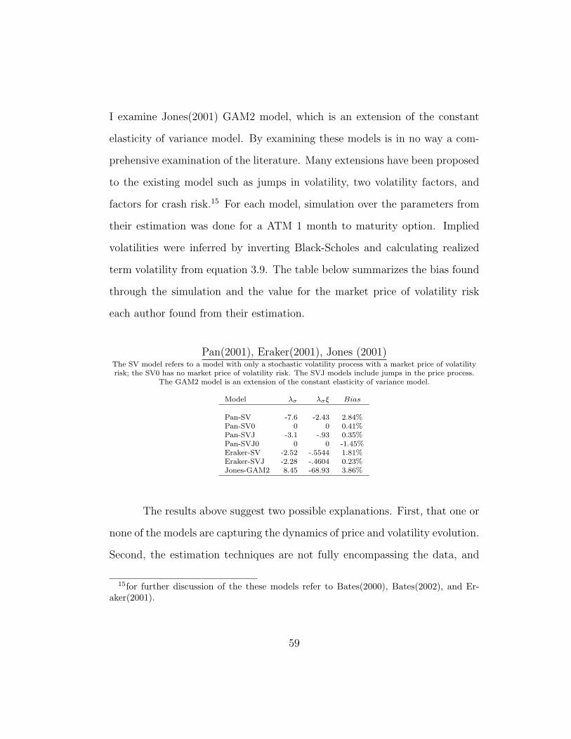
I examine Jones(2001) GAM2 model, which is an extension of the constant
elasticity of variance model. By examining these models is in no way a com-
prehensive examination of the literature. Many extensions have been proposed
to the existing model such as jumps in volatility, two volatility factors, and
factors for crash risk.15 For each model, simulation over the parameters from
their estimation was done for a ATM 1 month to maturity option. Implied
volatilities were inferred by inverting Black-Scholes and calculating realized
term volatility from equation 3.9. The table below summarizes the bias found
through the simulation and the value for the market price of volatility risk
each author found from their estimation.
Pan(2001), Eraker(2001), Jones (2001)The SV model refers to a model with only a stochastic volatility process with a market price of volatilityrisk; the SV0 has no market price of volatility risk. The SVJ models include jumps in the price process.
The GAM2 model is an extension of the constant elasticity of variance model.
Model λσ λσξ Bias
Pan-SV -7.6 -2.43 2.84%Pan-SV0 0 0 0.41%Pan-SVJ -3.1 -.93 0.35%Pan-SVJ0 0 0 -1.45%Eraker-SV -2.52 -.5544 1.81%Eraker-SVJ -2.28 -.4604 0.23%Jones-GAM2 8.45 -68.93 3.86%
The results above suggest two possible explanations. First, that one or
none of the models are capturing the dynamics of price and volatility evolution.
Second, the estimation techniques are not fully encompassing the data, and
15for further discussion of the these models refer to Bates(2000), Bates(2002), and Er-aker(2001).
59

arrive at distorted parameter estimates. While it appears that the higher in
terms of absolute value the market price of volatility risk is, the higher the bias
becomes, this effect diminishes when jump parameters are included. A direct
relationship between market price of volatility risk and the bias in BSIV can
not be made without examining the effect of the other parameters, especially
ξ. Since λσ and ξ are multiplicative in the volatility process, it is important
to examine the combined effect of the two values on the bias. As the above
table shows, all the values are less than or equal to zero, and are negatively
correlated with the positive bias. In fact, Pan’s SVJ0 model, which has the
best model fit, produces a negative bias with a zero market price of volatility
risk, further suggesting the importance of the parameter.
The best candidates above based solely on the bias results appear to
be Jones GAM2, Pan-SV, and Eraker SVJ model. However, as noted by the
authors these models underperform when it comes to model fit as compared
to the SVJ model. Jones’ model does not incorporate any jumps, and his ξ
parameter seems to be to high as compared with previous results. The prior
simulation shows that using the traditional Bates model as a framework, one
can input appropriate parameters and arrive at the desired results. So, the
question arises to where the breakdown in estimation came from in arriving
at implausible parameters in fitting the model.
60

3.3 Estimation
3.3.1 Simulation within a Simulation
There has been much space devoted recently in the literature to empir-
ically testing the feasibility of these parametric models. The main issue faced
is recovering the latent spot volatility, which precludes the possibility of writ-
ing a likelihood function. Some authors such as Chernov and Ghysels (2002)
have implemented Galant and Tauchen EMM (1998) methodology, while Pan
(2000) applied “implied-state” GMM to estimate the parameters, and Jones
(2001) used a Bayesian approach. I adopt a different philosophy. Since the
intent differs from prior studies, I will use the historical BSIV and a proxy for
realized term volatility in the estimation procedure. To verify that I can link
these two estimates to the original underlying process, I generate the results
through a multi-simulation procedure.
Both the risk-neutral and real-world processes should have the same
instantaneous spot volatility, but the 1 month estimates of volatility should be
distinct for the two processes due to the various risk factors. Thus any 30 day
estimate of true Black-Scholes implied volatility should contain information
regarding the magnitude and direction of the jump size, jump intensity, and
market price of volatility risk factors. However, to attain these estimates it is
necessary to establish a link from the 30 day estimates to the original instan-
taneous κ, θ, and ξ. Additionally, the real-world volatility can be recovered if
the original instantaneous spot volatility is known.
To accomplish this I simulate the underlying model through time, start-
61
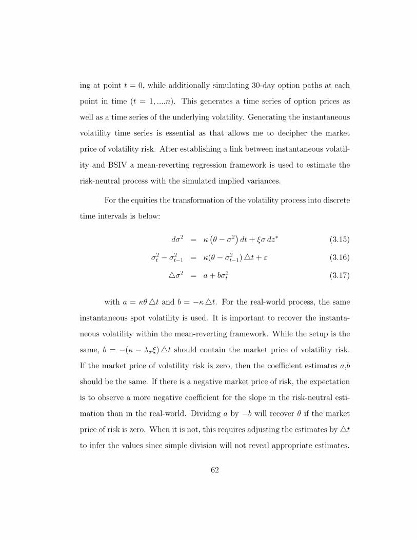
ing at point t = 0, while additionally simulating 30-day option paths at each
point in time (t = 1, ....n). This generates a time series of option prices as
well as a time series of the underlying volatility. Generating the instantaneous
volatility time series is essential as that allows me to decipher the market
price of volatility risk. After establishing a link between instantaneous volatil-
ity and BSIV a mean-reverting regression framework is used to estimate the
risk-neutral process with the simulated implied variances.
For the equities the transformation of the volatility process into discrete
time intervals is below:
dσ2 = κ(θ − σ2
)dt+ ξσ dz∗ (3.15)
σ2t − σ2
t−1 = κ(θ − σ2t−1)4t+ ε (3.16)
4σ2 = a+ bσ2t (3.17)
with a = κθ4t and b = −κ4t. For the real-world process, the same
instantaneous spot volatility is used. It is important to recover the instanta-
neous volatility within the mean-reverting framework. While the setup is the
same, b = −(κ − λσξ)4t should contain the market price of volatility risk.
If the market price of volatility risk is zero, then the coefficient estimates a,b
should be the same. If there is a negative market price of risk, the expectation
is to observe a more negative coefficient for the slope in the risk-neutral esti-
mation than in the real-world. Dividing a by −b will recover θ if the market
price of risk is zero. When it is not, this requires adjusting the estimates by 4t
to infer the values since simple division will not reveal appropriate estimates.
62
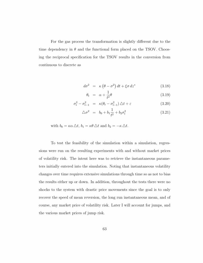
For the gas process the transformation is slightly different due to the
time dependency in θ and the functional form placed on the TSOV. Choos-
ing the reciprocal specification for the TSOV results in the conversion from
continuous to discrete as
dσ2 = κ(θ − σ2
)dt+ ξσ dz∗ (3.18)
θt = α+1
t2θ (3.19)
σ2t − σ2
t−1 = κ(θt − σ2t−1)4t+ ε (3.20)
4σ2 = b0 + b11
t2+ b2σ
2t (3.21)
with b0 = κα4t, b1 = κθ4t and b2 = −κ4t.
To test the feasibility of the simulation within a simulation, regres-
sions were run on the resulting experiments with and without market prices
of volatility risk. The intent here was to retrieve the instantaneous parame-
ters initially entered into the simulation. Noting that instantaneous volatility
changes over time requires extensive simulations through time so as not to bias
the results either up or down. In addition, throughout the tests there were no
shocks to the system with drastic price movements since the goal is to only
recover the speed of mean reversion, the long run instantaneous mean, and of
course, any market price of volatility risk. Later I will account for jumps, and
the various market prices of jump risk.
63

The initial test had no market price of volatility risk; the intent here
was to show that the recovered instantaneous volatility was the same as the
implied volatility from inverting Black-Scholes from call and put prices. I
am at present ignoring the potential arbitrage opportunity by forcing a zero
market price of volatility risk since the goal is to show the validity in the
simulation within a simulation technique. The second regression is the result
of a -2 value for the market price of volatility risk. All other parameters are
the same.
Table 18 shows the results of the mean reversion regression. By divid-
ing the coefficients in the regression κ, θ, and the market price of volatility
risk was recovered. For a process with no market price of volatility risk t-tests
revealed that the BSIV from the 30-day option was not significantly different
as the underlying spot volatility even though the instantaneous spot volatility
is allowed to move on a daily basis. This is important since 30-day implied
volatility can be used as a proxy for the instantaneous spot volatility. When
there is a market price of volatility risk, the resulting slope coefficient is lower.
Given that the κ is 5.61, I can infer the type of effect that the market price of
risk has had on the resulting coefficient. Since finding the parameters through
simple division is not feasible, the ratio between the slope coefficients is ex-
amined for instances of the existence and absence of market price of volatility
risk. The resulting ratio is 1.62. From this value calibrating the model backed
out what value the market price of volatility risk had to be. T-tests revealed
that the value was not significantly different from -2 for the market price of
64
volatility risk given the other initial values in the estimation. What is also
observable is that recovered θ is the same for both processes, which is essen-
tial since the given instantaneous spot volatility is same for both simulations
even with different market prices of volatility risks. The given values in the
simulations were κ = 5.61, θ = 17.5%, ξ = .3, and ρ = −.53. The starting
stock price and strike price were set equal to 50 with a 4% risk free rate.
3.3.2 Estimation Using Mean Reverting Framework
Using the data described in section 2.2.1, and the mean reverting tech-
nique described earlier, I regressed the 30 day implied volatility series of the
S&P 100, S&P 500, and the gas contracts. For the S&P 100 the data was
split into pre- and post- October 87 crash samples. For the gas contracts it
was necessary to separate the contracts into individual months in the mean-
reverting framework to remove any seasonality effects. It was also necessary
to include year dummies, as there is a clear year effect for each contract. The
results are reported in tables 19 and 20.
Most of the slope and intercept coefficient are significant for the S&P
100, S&P 500 and each of the monthly gas contracts. Translating this into
actual values, multiplying b by 252, κ would be about 50.85 for the S&P 100
and 14.67 for the S&P 500. While 50.85 appears to be slightly high, it does
include the crash of October 87. The separate pre- and post- crash samples
have κ of 9.42 and 16.11 which appear more reasonable and highlight the
increased volatility present in the market post the October 87 crash. For the
65
gas contracts there is a much lower level of mean-reversion due to the presence
of the TSOV for all months. Months such as January that tend have very
large TSOV parameter estimates will result in smaller κ estimates since the
TSOV parameter is capturing the large ramping up of volatility.
The long run mean, θ, can be inferred by −ab. This results in an average
volatility of around 22.62% for the S&P 500 and 19.52% for the S&P 100. For
the gas contracts θ is equal to − b1b2
. It is apparent that the winter months
have much higher levels of volatility while the other months have volatility
levels similar to that of the S&P indices. This is quite intuitive given the
high demand for heating in these months. Solving for ξ is simply a matter
of examining the sum of squared errors from the regression, and adjusting
for the time and volatility factors. The values for ξ may be considered high
as compared to other models, but not accounting for jumps forces the model
to elevate ξ for better fit. Since there is no frame of reference for the gas
markets, equity values are used and could not be considered improper given
the similarity. Given these values, and relating them to the instantaneous
counterparts is all that remains is estimating λσ.
3.3.3 Estimation of λσ
Running regressions on the simulation within a simulation revealed that
the instantaneous underlying parameters were recovered from the 30 day im-
plied volatility estimates. This allows the use of the 30 day implied volatility
as a proxy for the latent instantaneous volatility. While observing that 30
66
day implied volatility does not equal instantaneous volatility, it can be used
as a legitimate proxy given the numerical evidence shown in the simulation
with a simulation. However, I was unable to recover the same parameters using
the realized volatility even given the market price of volatility risk adjustment.
This presented a problem in estimating the market price of volatility risk since
the instantaneous volatility is needed for both processes. This problem is cir-
cumvented by using the knowledge of the biased nature of implied volatility
as a predictor of future realized volatility. Given the estimations done earlier,
there is a proportional bias of around 73.5%. Using the estimates from the
mean-reversion regression done on 30-day implied volatility and the propor-
tional bias, the market price of volatility risk is recovered through calibration.
In addition, the actual bias for any particular time period can be used, i.e. the
pre-Oct 87 crash BSIV bias levels to find a λσ for that period. This generates
a time-series of λσ, which in turn generates appropriate significance for the
estimates.
This same process is replicated for the gas contracts, but with the
added complication of the TSOV. I adjust the mean-reversion regression by
incorporating the time component for theta. Substituting in for θ eliminates
the intercept term and results in two time dependent regressors. However, the
added complication of contract specific volatilities requires separating each
contract by month to find unique parameters for each monthly contract. The
steps in the estimation are outlined below
1. Divide the sample into non-overlapping intervals
67

2. Run variance regressions to obtain κ, θ, and ξ for each sub period
3. Calculate bias between implied volatility and realized volatility for that
period using either a) the results from bias regression earlier or b) actual
data from that period
4. Using known parameters and bias in BSIV/BIV, calibrate model to find
λσ
5. Compute mean and standard deviation for λσ to obtain significance
While the calibration method in backing out lambda achieves reason-
able estimates, it is necessary to gather some measure of statistical significance
for these measures. By estimating multiple lambda’s within sub-samples al-
lows me to generate confidence intervals for the parameter. To account for
overlapping estimation periods, adjustments for correlations were made by
using the number of days in common. The correlation is modeled as such
Let
Xi ∼ N(µ, σ2)
Corr(Xi, Xj) =
{kn, if k > 0
0, if k = 0
where n is the number of days over which λσ are estimated and k is
the number of days in common. Now consider the traditional estimator of
variance given by
68
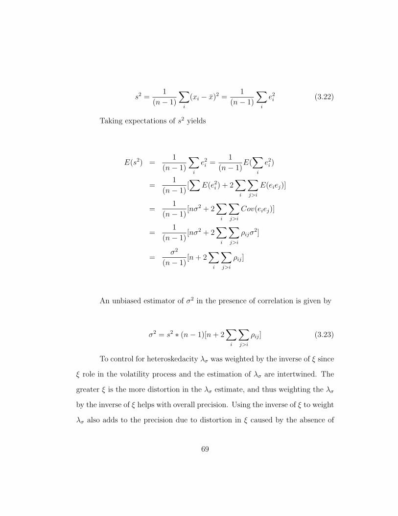
s2 =1
(n− 1)
∑i
(xi − x̄)2 =1
(n− 1)
∑i
e2i (3.22)
Taking expectations of s2 yields
E(s2) =1
(n− 1)
∑i
e2i =1
(n− 1)E(∑
i
e2i )
=1
(n− 1)[∑
E(e2i ) + 2∑
i
∑j>i
E(eiej)]
=1
(n− 1)[nσ2 + 2
∑i
∑j>i
Cov(eiej)]
=1
(n− 1)[nσ2 + 2
∑i
∑j>i
ρijσ2]
=σ2
(n− 1)[n+ 2
∑i
∑j>i
ρij]
An unbiased estimator of σ2 in the presence of correlation is given by
σ2 = s2 ∗ (n− 1)[n+ 2∑
i
∑j>i
ρij] (3.23)
To control for heteroskedacity λσ was weighted by the inverse of ξ since
ξ role in the volatility process and the estimation of λσ are intertwined. The
greater ξ is the more distortion in the λσ estimate, and thus weighting the λσ
by the inverse of ξ helps with overall precision. Using the inverse of ξ to weight
λσ also adds to the precision due to distortion in ξ caused by the absence of
69
jump parameters. When ξ is large, there is greater probability that it has been
mismeasured due to the exclusion of any potential jumps in the model.
The estimates for the monthly λσ are below. For the S&P 500/S&P
100 the lambda’s are negative and statistically significant. The S&P 100 has
a higher overall bias based on a longer time set that involved the October 87
crash and prior. This period has been documented with very expensive out
of the money puts suggesting a larger market price of volatility risk as well as
larger jump premiums. Each monthly gas contract’s λσ are negative and are
significant at the 5% level. The winter months tend to have higher lambda’s
than the other months which follows the typical seasonality patterns that the
winter months are more volatile, experience more jumps, and tend to have a
higher degree of bias in implied volatility. These Sharpe ratios are relativly
high, and must be interpreted with caution. While authors such as Bates
(2000) and Bakshi and Kapadia (2002) document the significant premium
extracted from selling option, the results in the table below do not account
for jump premiums. The premiums are slightly inflated since the model has
to account for large daily price movements by increasing ξ. Typically when
fitting a stochastic volatility model without jumps ξ will be higher due to the
excess kurtosis in option prices. This results in distorted λσ. However, while
not concerned with option model fit at this moment, just including stochastic
volatility can improve model fit by almost 70% over the Black-Scholes model.
In addition, since I am only looking at ATM options, and the most significant
jump premiums occur for ITM (OTM) calls (puts) for equities and OTM calls
70
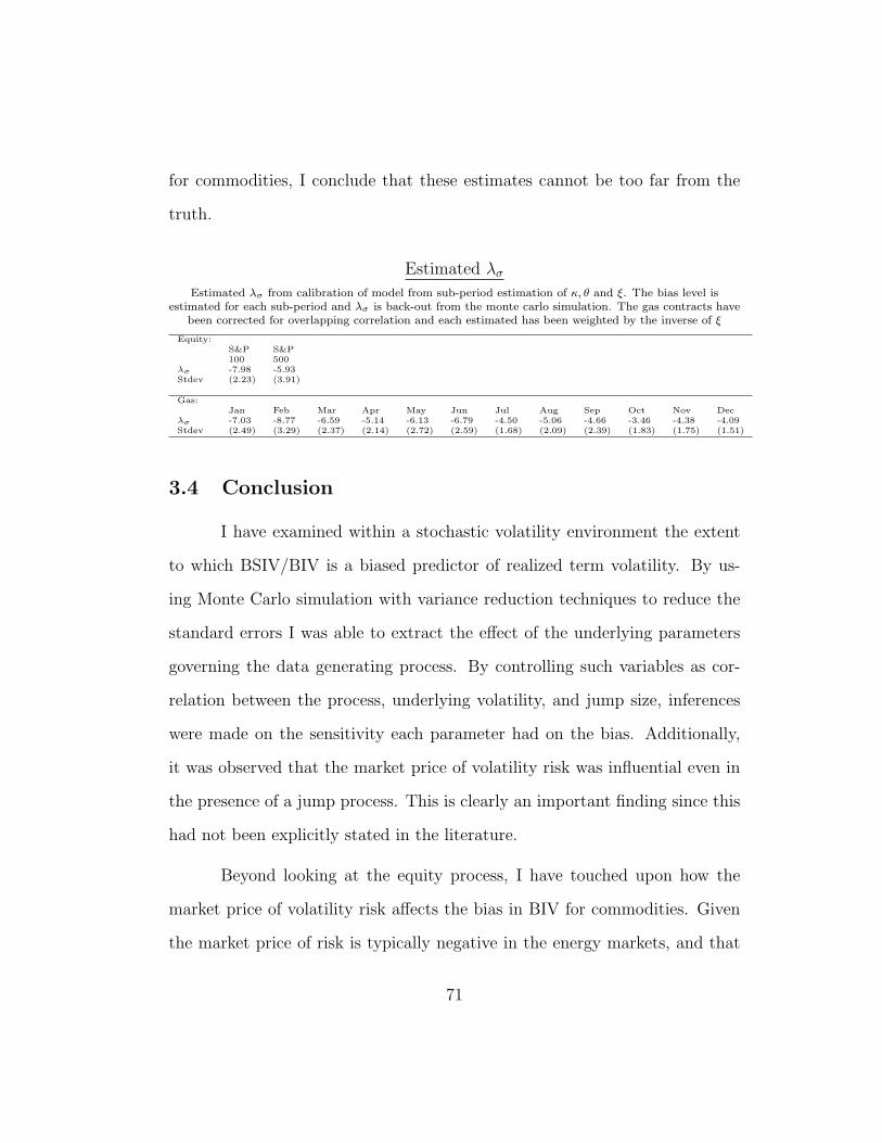
for commodities, I conclude that these estimates cannot be too far from the
truth.
Estimated λσ
Estimated λσ from calibration of model from sub-period estimation of κ, θ and ξ. The bias level isestimated for each sub-period and λσ is back-out from the monte carlo simulation. The gas contracts have
been corrected for overlapping correlation and each estimated has been weighted by the inverse of ξ
Equity:S&P S&P100 500
λσ -7.98 -5.93Stdev (2.23) (3.91)
Gas:Jan Feb Mar Apr May Jun Jul Aug Sep Oct Nov Dec
λσ -7.03 -8.77 -6.59 -5.14 -6.13 -6.79 -4.50 -5.06 -4.66 -3.46 -4.38 -4.09Stdev (2.49) (3.29) (2.37) (2.14) (2.72) (2.59) (1.68) (2.09) (2.39) (1.83) (1.75) (1.51)
3.4 Conclusion
I have examined within a stochastic volatility environment the extent
to which BSIV/BIV is a biased predictor of realized term volatility. By us-
ing Monte Carlo simulation with variance reduction techniques to reduce the
standard errors I was able to extract the effect of the underlying parameters
governing the data generating process. By controlling such variables as cor-
relation between the process, underlying volatility, and jump size, inferences
were made on the sensitivity each parameter had on the bias. Additionally,
it was observed that the market price of volatility risk was influential even in
the presence of a jump process. This is clearly an important finding since this
had not been explicitly stated in the literature.
Beyond looking at the equity process, I have touched upon how the
market price of volatility risk affects the bias in BIV for commodities. Given
the market price of risk is typically negative in the energy markets, and that
71
prices and volatility tend to be positively correlated, I have found that the
market price of volatility risk for natural gas contracts is also negative. The
direction of the bias in BIV on realized term volatility is also upward, and the
magnitude may be higher than that of the equity process.
While the empirical test focused only on the stochastic volatility pro-
cess, I have simulated various models that incorporated jumps. From these
results it was determined that jump risk factors are not the only priced fac-
tor when it comes to option values. Jump models without priced stochastic
volatility factors cannot explain the full degree of bias present in Black-Scholes
implied volatility.
The empirical tests performed by Christensen and Prabhala (1998) fo-
cused on index options, and while I replicate their results for the S&P 100 and
S&P 500, the main focus is on the bias in gas contracts. The complication of
examining gas contracts lies in the significant TSOV and seasonality tests. I
am able to demonstrate the upward bias nature in BIV, and link this bias to
the market price of volatility risk.
The resulting empirical tests for λσ revealed that the factor is negative
and significant for both the equity and gas process. I have introduced a tech-
nique to link the latent volatility factor to the implied volatility from a 30 day
option contract which allowed for simple estimation of λσ. The major con-
clusion is that the market price of volatility risk is an important price factor,
and lends explanation to why option traders tend to be short. This effect is
especially noticeable in the gas contracts, where the high load months in the
72

winter experience higher risk premiums.
The work in this area is still incomplete. It is necessary to test these
results further, especially for the gas contracts. Can these results hold up to the
non-parametric tests of Bakshi and Kapadia (2001) and Coval and Shumway
(2000)? Additionally, what happens when ITM and OTM options are included
in the data, and when jumps are included in the price process. I address these
issues in the following chapter with a test for model fit for various parametric
option model candidates as well as infer the multiple market prices of risk.
73
Chapter 4
Empirical Performance of Option Models for
Natural Gas and Estimation of the Market
Price(s) of Risk
4.1 Introduction
The intent of this chapter is to examine in greater detail the dynamics of
the natural gas markets. This first entails estimation of the implicit parameters
underlying a variety of option models to capture cross-sectional performance.
This estimation will not only reveal how mis-specified the Black (1976) option
model is, but also tells by comparison how well certain models do fit the data.
This leads directly into further estimation on the market price of volatility
risk by incorporating the risk-neutral estimates from the model performance
analysis. With the inclusion of jumps to the model, errors caused by model
misspecification are minimized and the full cross-section of option price data
can be utilized to infer the priced risk factors.
The current state of option pricing offers a wide range of models that
relax the assumptions of the Black-Scholes model. The models of Hull and
White (1987), Heston(1993), Melino and Turnbull(1991, 1995), and Stein and
Stein (1991) have expanded upon Black-Scholes by dropping constant volatility
in favor of stochastic volatility. The stochastic volatility model was better able
74

to capture the skewness in option prices, resulting in improvement of Black-
Scholes in terms of model fit, through the correlation between the price and
volatility processes and variation in volatility. Bates (1996) and Scott (1997)
added return-jumps to the framework, allowing the model to capture skewness
without adversely affecting kurtosis. The inclusion of return jumps had the
additional impact in less over-parameterization error due to less reliance on
volatility variation to capture short-term volatility skews. This is shown in
the works of Bakshi, Cao and Chen (1997) and Pan (2000). The most current
extensions to the model have been the inclusion of volatility-jumps by Duffie,
Pan, and Singleton (2000), and crash risk by Bates (2003). The benefits to
volatility-jumps are shown in Bakshi and Cao (2003), who test the sample
on individual equity options. Most empirical tests completed have examined
option model performance in terms of equity and index options. While our
knowledge is quite extensive for this market, the results for equities are not
directly transferable to other markets, such as foreign exchange contracts and
commodities futures. The first goal of this chapter is to examine the perfor-
mance of these option models to assess overall fit and capture the risk-neutral
dynamics of natural gas option contracts.
By comparison very little is known about the commodities market in
term of option pricing and empirical performance of various option models.
Empirically, there is observed positive skewness in Black implied volatilities,
higher levels of volatility, and a potential negative market price of risk. These
factors contribute to a distinct market and require a better understanding of
75

how to model commodities option pricing. To explore empirical and mod-
eling aspects of commodity options, I will test a variety of models, start-
ing with Black-Scholes/Black and working up to the Duffie, Pan, and Sin-
gleton (2000) model accommodating stochastic volatility, return-jumps, and
volatility-jumps. The advantage of testing this type of model is that it in-
corporates the stochastic volatility model of Heston (1993) and the stochastic
volatility with return-jumps model of Bates (1996). In addition, I test the
stochastic volatility with jumps model (SVJ) with the additional adjustment
for the term-structure of volatility. As the option approaches maturity, there is
an observed significant “ramping up” of implied volatility. In the commodities
market where there is such a significant TSOV, the addition of term structure
parameter implicit within the model seems like a natural extension.
Each model in evaluated on in-sample performance, cross-sectional per-
centage pricing errors, and 2 out-of-sample metrics. The percentage pricing
errors are generated using the structural parameter estimates including the
implied volatility, and the given futures price, strike price, risk-free rate, and
time to maturity for that day. The out-of-sample tests use the 1-day and 5-day
behind implied parameters to price the current day option value. These tests
provide direct evidence for model misspecification and will penalize a more
complex model for overfitting.
Based on the sample of 98,006 usable closing option prices from Jan
1999 to October 2002, I find that incorporating a TSOV effect demonstrates
little improvement over the Bates (1996) model, while adding independent
76

volatility jumps to the Bates model has the best overall performance. Similar
to the results for equities, the stochastic volatility model of Heston (1993) im-
proves in-sample performance by close to 50% as compared to the Black model
for the full sample. The inclusion of return-jumps, and subsequently volatility-
jumps, further improves upon the Heston model, but in smaller increments.
Controlling for seasonality and year effects dramatically changes the structural
parameter estimates, as volatility variation, process correlation, and jump size
appear to be yearly and monthly dependent. The winter months especially
show large positive correlation and mean jump size. The 2000 expiration con-
tracts show tremendous volatility variation and high positive correlation in
part due to the energy shortage and deregulation. These effect are model
independent. However, volatility variation dramatically declines when return
jumps are included. This is quite telling as the Bates model tends to improves
model fit for OTM short-term calls as well as reducing the pricing bias for
OTM long-term calls. Surprisingly, the correlated double jump model is out
performed by the independent double jump model across all years and sea-
sons. The parameter values indicate that the double-jump model shows close
to a zero correlation between return and volatility-jumps. While the indepen-
dent double jump model is a nested model, the arrival rates for the return
and volatility-jumps are independent, possibly explaining the improved in and
out-of-sample model performance.
The second objective is to confirm a negative market price of volatility
risk for commodities. The findings of the previous chapter suggest a negative
77
market price of volatility risk for both equities and commodities. The results
for equities are confirmed by the non-parametric tests of Bakshi and Kapadai
(2000) and Coval and Shumway (2001). Chapter 3 implemented a technique
to test a weighted average estimate of implied volatility by using a mean re-
verting stochastic volatility framework which calibrates the risk-neutral world
to the risk-neutral parameter estimates through the market prices of risk. The
findings for natural gas contracts show a significant and negative market price
of volatility risk for the entire sample and each monthly contract. However, the
relative model misspecification by ignoring return-jumps forces the volatility
variation to capture most of the upper moments. This results in an upward-
bias estimate of the market price of volatility risk since the implied volatility
estimate ignores the full cross-section of option prices. In this study, I use the
structural parameter estimates from the model performance estimation and
Monte Carlo simulation to combine the risk-neutral and real-world distribu-
tions to solve for the market prices of risk. This is accomplished by jointly
minimizing an objective function that takes the difference between the actual
volatility and model estimated volatility as well as the Black implied volatil-
ities and model estimated implied volatility. The resulting estimation of the
risk factors is improved by incorporating the cross-section as well as the time
series of spot and option prices. Allowing for return-jumps places less restric-
tion on the stochastic volatility parameters, resulting in improved estimation
and minimizes the error resulting from model misspecification.
Of equal importance is to resolve the mystery of the direction of the risk
78

premia for natural gas contracts. To this point there has been no conclusive
finding that can pinpoint the sign and magnitude either through a lack of data
or degree of volatility inherent in the contracts. Through this technique I hope
to shed further light on this estimation.
I plan to address the following questions.
• Which model best fits the positive skewness and high kurtosis present in
the risk-neutral distributions of commodities prices
• How much does TSOV matter in model fit
• How are the parameter estimates distinct from those typically found for
equity index options
• What are the market price(s) of risk, especially the market price of
volatility risk
The chapter is organized as follows. Section 2 presents the double-jump
option-pricing model and all other models to be investigated with the added
TSOV adjustment. Section 3 describes empirical issues and the construction
of the option sample. Section 4 describes the estimation procedure,in-sample
option model fit results, and out-of-sample results. Section 5 and 6 focus
on the estimation technique and the market prices of risk. Conclusions are
provided in Section 7.
79

4.2 Modeling Issues
I present a closed-form option-pricing model similar to that of Pan
(2000) and Bates (1996), but in addition add in time dependence to the level
to which volatility reverts to. The addition of the time dependence of volatil-
ity model with all those considered in Bakshi, Cao, and Chen (1997), Bates
(2000), and Pan (2000), forms the basis for empirical comparisons. Bakshi,
Kapadia, and Madan (2003) provide theoretical foundations for the existence
of less negatively-skewed and fat-tailed individual risk-neutral distributions for
firm equity options. They argue that kurtosis is a fundamental determinant
of option prices when the risk-neutral distributions are less skewed. This al-
lowed Bakshi and Cao (2003) to implement the double-jump option-pricing
model where return-jumps and volatility-jumps are the primary source of ex-
cess kurtosis. However, the knowledge is less complete for commodity options
and requires the testing of the prior models along with the alternative model
incorporating the TSOV. I can make no such claim about the source of excess
kurtosis, especially since there is a fair degree of skewness. This skewness,
which is mostly positive, has had occurrences of severe negative skewness for
periods during the 2000 and 2001 expiration contracts.
4.2.1 Data Generating Process for the Double Jump Model
I will ensue with a quick review of the double-jump option model under
stochastic volatility as in Duffie, Pan, and Singleton (2000) for completeness.
The underlying non-dividend-paying futures price, Ft, is governed by the follow
80
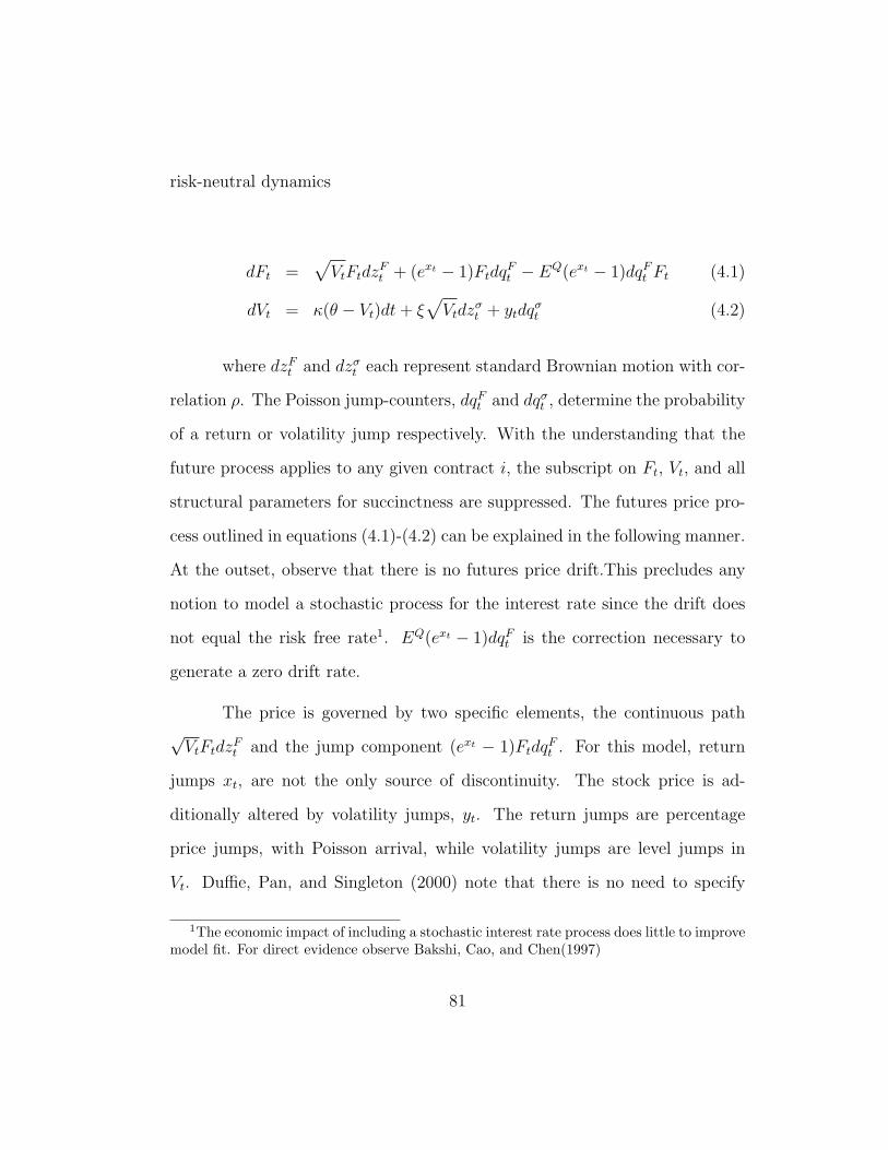
risk-neutral dynamics
dFt =√VtFtdz
Ft + (ext − 1)Ftdq
Ft − EQ(ext − 1)dqF
t Ft (4.1)
dVt = κ(θ − Vt)dt+ ξ√Vtdz
σt + ytdq
σt (4.2)
where dzFt and dzσ
t each represent standard Brownian motion with cor-
relation ρ. The Poisson jump-counters, dqFt and dqσ
t , determine the probability
of a return or volatility jump respectively. With the understanding that the
future process applies to any given contract i, the subscript on Ft, Vt, and all
structural parameters for succinctness are suppressed. The futures price pro-
cess outlined in equations (4.1)-(4.2) can be explained in the following manner.
At the outset, observe that there is no futures price drift.This precludes any
notion to model a stochastic process for the interest rate since the drift does
not equal the risk free rate1. EQ(ext − 1)dqFt is the correction necessary to
generate a zero drift rate.
The price is governed by two specific elements, the continuous path√VtFtdz
Ft and the jump component (ext − 1)Ftdq
Ft . For this model, return
jumps xt, are not the only source of discontinuity. The stock price is ad-
ditionally altered by volatility jumps, yt. The return jumps are percentage
price jumps, with Poisson arrival, while volatility jumps are level jumps in
Vt. Duffie, Pan, and Singleton (2000) note that there is no need to specify
1The economic impact of including a stochastic interest rate process does little to improvemodel fit. For direct evidence observe Bakshi, Cao, and Chen(1997)
81
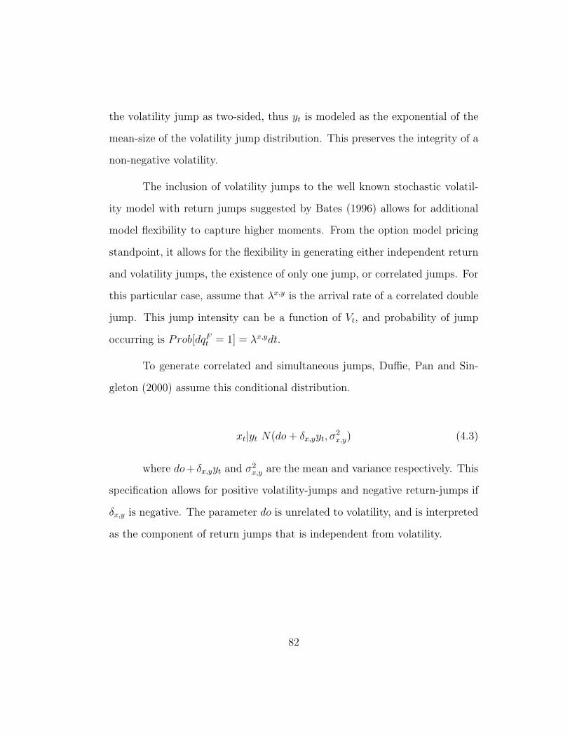
the volatility jump as two-sided, thus yt is modeled as the exponential of the
mean-size of the volatility jump distribution. This preserves the integrity of a
non-negative volatility.
The inclusion of volatility jumps to the well known stochastic volatil-
ity model with return jumps suggested by Bates (1996) allows for additional
model flexibility to capture higher moments. From the option model pricing
standpoint, it allows for the flexibility in generating either independent return
and volatility jumps, the existence of only one jump, or correlated jumps. For
this particular case, assume that λx,y is the arrival rate of a correlated double
jump. This jump intensity can be a function of Vt, and probability of jump
occurring is Prob[dqFt = 1] = λx,ydt.
To generate correlated and simultaneous jumps, Duffie, Pan and Sin-
gleton (2000) assume this conditional distribution.
xt|yt N(do+ δx,yyt, σ2x,y) (4.3)
where do+ δx,yyt and σ2x,y are the mean and variance respectively. This
specification allows for positive volatility-jumps and negative return-jumps if
δx,y is negative. The parameter do is unrelated to volatility, and is interpreted
as the component of return jumps that is independent from volatility.
82
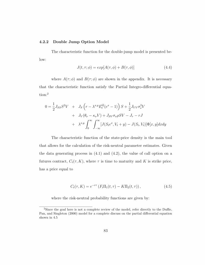
4.2.2 Double Jump Option Model
The characteristic function for the double-jump model is presented be-
low:
J(t, τ ;φ) = exp[A(τ, φ) +B(τ, φ)] (4.4)
where A(τ ;φ) and B(τ ;φ) are shown in the appendix. It is necessary
that the characteristic function satisfy the Partial Integro-differential equa-
tion:2
0 =1
2JSSS
2V + JS
(r − λx,yEQ
t (ex − 1))S +
1
2JV V σ
2νV
+ JV (θν − κνV ) + JSV σνρSV − Jτ − rJ
+ λx,y
∫ ∞
0
∫ ∞
−∞[J(Ste
x, Vt + y)− J(St, Vt)]Φ[x, y]dxdy
The characteristic function of the state-price density is the main tool
that allows for the calculation of the risk-neutral parameter estimates. Given
the data generating process in (4.1) and (4.2), the value of call option on a
futures contract, Ct(τ,K), where τ is time to maturity and K is strike price,
has a price equal to
Ct(τ,K) = e−rτ (FtΠ1(t, τ)−KΠ2(t, τ)) , (4.5)
where the risk-neutral probability functions are given by:
2Since the goal here is not a complete review of the model, refer directly to the Duffie,Pan, and Singleton (2000) model for a complete discuss on the partial differential equationshown in 4.5
83
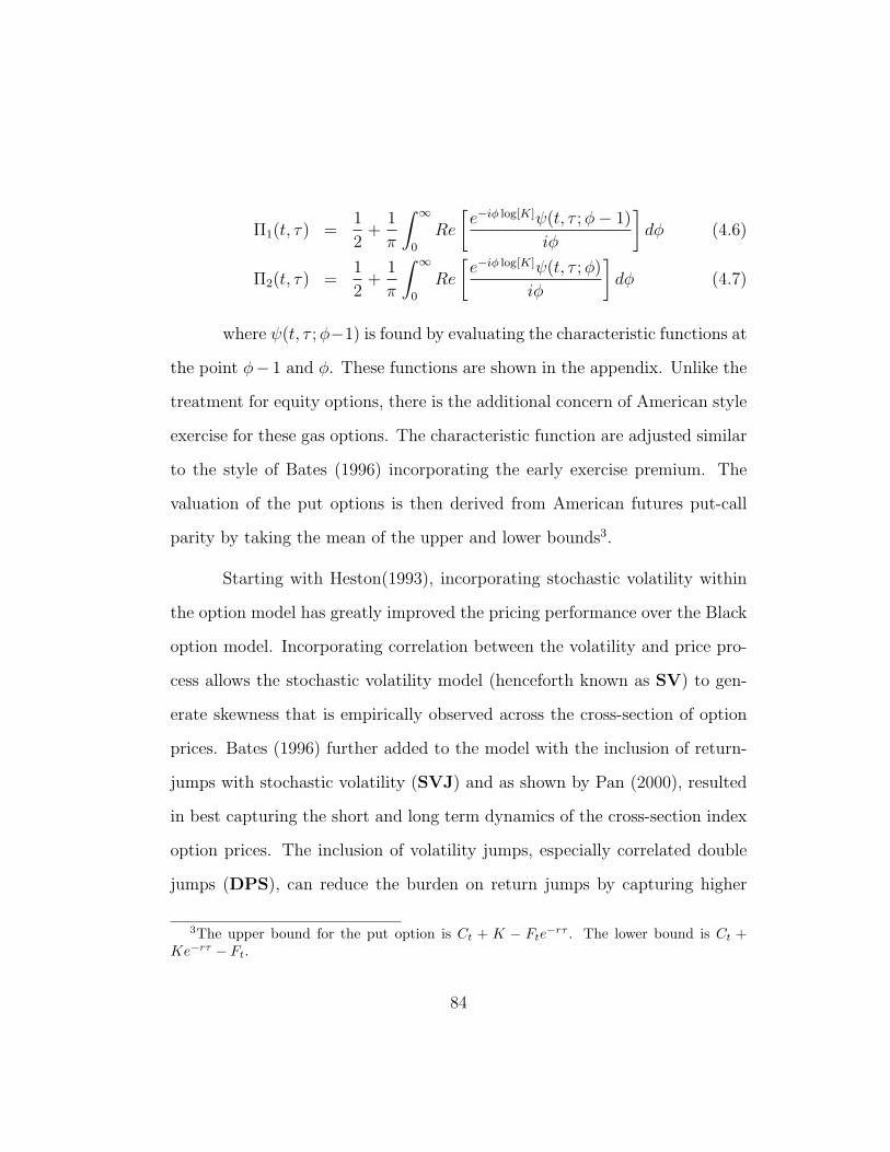
Π1(t, τ) =1
2+
1
π
∫ ∞
0
Re
[e−iφ log[K]ψ(t, τ ;φ− 1)
iφ
]dφ (4.6)
Π2(t, τ) =1
2+
1
π
∫ ∞
0
Re
[e−iφ log[K]ψ(t, τ ;φ)
iφ
]dφ (4.7)
where ψ(t, τ ;φ−1) is found by evaluating the characteristic functions at
the point φ− 1 and φ. These functions are shown in the appendix. Unlike the
treatment for equity options, there is the additional concern of American style
exercise for these gas options. The characteristic function are adjusted similar
to the style of Bates (1996) incorporating the early exercise premium. The
valuation of the put options is then derived from American futures put-call
parity by taking the mean of the upper and lower bounds3.
Starting with Heston(1993), incorporating stochastic volatility within
the option model has greatly improved the pricing performance over the Black
option model. Incorporating correlation between the volatility and price pro-
cess allows the stochastic volatility model (henceforth known as SV) to gen-
erate skewness that is empirically observed across the cross-section of option
prices. Bates (1996) further added to the model with the inclusion of return-
jumps with stochastic volatility (SVJ) and as shown by Pan (2000), resulted
in best capturing the short and long term dynamics of the cross-section index
option prices. The inclusion of volatility jumps, especially correlated double
jumps (DPS), can reduce the burden on return jumps by capturing higher
3The upper bound for the put option is Ct + K − Fte−rτ . The lower bound is Ct +
Ke−rτ − Ft.
84
third or fourth moments when necessary. For example, to achieve more posi-
tive skewness without restricting excess kurtosis, an upward jump in volatility
is accompanied by an upward return jump when δx,y > 0. This is especially
important for gas options for two reasons. First, besides empirical observa-
tions, there is little understanding in terms of structural parameter estimation
and option model performance. Hereto, it is necessary to test each model to
gain further insight into this market. Second, the market is highly volatile
as compared to equities with large volatility skews/smiles at various maturi-
ties. This requires added option model flexibility even beyond equity option
estimation.
4.2.3 Independent Double Jumps and TSOV considerations
As mentioned earlier, the SV and SVJ models are contained within the
double jump model. They are directly attained from the the double jump
model when the volatility and return jumps are independent. This results in
separate jump arrivals such that λx is the arrival rate for return-jumps and
λy is the arrival rate for volatility-jumps4. The characteristic functions for the
independent double jump model are shown in the appendix. To generate the
Heston (1993) model, setting λx = 0 and λy = 0 within (SVDJ) will result
in no return or volatility jumps. For SVJ, restricting to λy = 0 generates
only return jumps. Within this chapter, I have not examined the case of
volatility only jumps, (SVJV), given the results shown in Bakshi and Cao
4Bakshi and Cao (2003) suggest the return jump distribution as x N(log(1+µx)− 12σ2
x, σ2x)
85
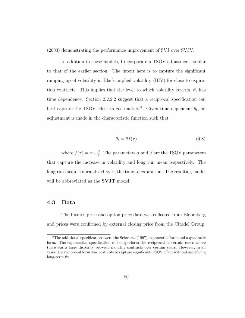
(2003) demonstrating the performance improvement of SVJ over SVJV.
In addition to these models, I incorporate a TSOV adjustment similar
to that of the earlier section. The intent here is to capture the significant
ramping up of volatility in Black implied volatility (BIV) for close to expira-
tion contracts. This implies that the level to which volatility reverts, θ, has
time dependence. Section 2.2.2.2 suggest that a reciprocal specification can
best capture the TSOV effect in gas markets5. Given time dependent θt, an
adjustment is made in the characteristic function such that
θt = θf(τ) (4.8)
where f(τ) = α+ βτ. The parameters α and β are the TSOV parameters
that capture the increase in volatility and long run mean respectively. The
long run mean is normalized by τ , the time to expiration. The resulting model
will be abbreviated as the SVJT model.
4.3 Data
The futures price and option price data was collected from Bloomberg
and prices were confirmed by external closing price from the Citadel Group.
5The additional specifications were the Schwartz (1997) exponential form and a quadraticform. The exponential specification did outperform the reciprocal in certain cases wherethere was a large disparity between monthly contracts over certain years. However, in allcases, the reciprocal form was best able to capture significant TSOV effect without sacrificinglong-term fit.
86

The futures and option prices are daily closing prices for the January 2000
contract through the August 2003 contract. The final collected option price
is for the August 2003 contract with 305 days until expiration. The typical
contract has usable observation from 360 days until maturity for strike prices
from $2 to $8 over 5 cent increments. For estimation purposes, I examine
all calls and puts on each monthly contract from January 1st, 1999 through
October 26, 2002. Unlike equity index options, I have to be concerned with
liquidity issues since there are low volume and wide bid-ask spreads for many
strike prices. In estimation, strike prices with bid-ask spreads greater than
$0.25 will not be included. Additionally, commodity options are American
style exercised and most current options models can only handle a European
payoff. This can be controlled for in two ways. The first is to implement
the methodology adopted by Bakshi and Cao (2003), whereto restricting the
sample to short-term maturity out-of-the money options minimizes the chance
of early exercise. The second technique is to adopt the Barone-Adesi and
Whaley (1987) technique implemented by Bates (1996). As shown in the
appendix, I choose to adopt this technique to increase the sample of options
tested. By adopting the first method, the sample would be reduced down
from 98,006 usable observations to 23,074, substantially reducing the power of
future tests.
This data allows for the possibility of testing over many years as well
as within years. From the prior section it has been shown that there is a
significant term structure of volatility for gas contracts, and it may be more
87
appropriate to test these contracts on a yearly basis versus grouping each
year together. It is also noted that each month has a specific TSOV, which
additionally requires testing each month separately. Consequently, results will
show model fit and structural parameter estimations for both seasonal and
yearly results.
The prices collected are closing prices which are taken to be the mid-
point of the bid-ask spread. I exclude prices which are less than 3/8 of a
dollar, and prices that occur within 7 days of term. These restrictions are
greater than those reported by Bakshi and Cao (2003) since there are stronger
liquidity concerns with commodity options. Finally, all quotes not satisfying
the arbitrage condition are omitted.
Of the 98,006 observations, 46%(54%) of the observation were calls(puts).
For option maturity, there are 25%, 56%, and 19% observations when the
sample is divided into expirations of >180 days, 60-180 days, and <60 days
respectively. By moneyness, the sample is partitioned into 5 groups, deep out-
of-money (DOTM), out-of-money (OTM), at-the-money (ATM), in-the-money
(ITM), and deep in-the-money (DITM). The observations for each group are
5%, 18%, 25%, 27%, and 25%, where the bounds for DOTM, OTM, ATM,
ITM, and DITM calls(puts) are a strike/spot ratio > 1.2 (<.8), 1.05-1.2 (.8-
.95), .95-1.05, .8-.95 (1.05-1.2), and <.8 (>1.2) respectively.
88
4.3.1 Understanding the volatility in gas markets
A closer look at table 2 reveals volatility levels of daily futures price
changes of approximately 25% for any given month over 10 years. These
statistics are misleading since they do not reflect the variability of any given
contract for a given year or the degree of variability of different time periods
within a given contract. For example, using the data in 2.2.2.1, a closer look
at the February gas futures contract reveals yearly variations as high as 39% in
1997 and as low as 22% in 1992. Within time periods the average daily return
variation for 0-60 days till expiration is 55%, for 60-180 days it was 24%,
and for 180-360 days it was 15%. The February 2001 contract experienced
around 90% volatility for the short-term period of the contract as compared
to 13% volatility for the period from 180-360 days. The variation in sub-
period volatilities shows an increase from the early contracts (1991-1996) to
more recent contract years (1997-2003), and this increase is observable for each
month.
The potential measurement error issues that arise when dealing with es-
timation using option contracts require a closer look at the volume of contracts
traded and the bid/ask spread associated with each contract. If price of the
option contract is measured with error, the resulting inverted implied volatility
will be incorrectly estimated, and so to0 the risk-neutral parameter. The liq-
uidity issue is important because if there is minimal volume traded for a given
contract it could potentially result in sticky and non-informative prices. The
November futures contract tends on average to trade 254,000 weekly contracts
89

at the Bid price and 179,000 at the Ask price 6. By comparison the January
contracts trades a volume of 317,030 at the Ask price and 201,280 at the Bid
price. In terms of dollar weekly volume it equates to approximately $2,000mm
each week for any given monthly futures contract. It terms of bid/ask spreads,
the typical spread is on average around $.10 with a high of around $.30 for
any given month. For the options, the typical volume is much lower than the
futures contracts, and tends to increase as the option approaches maturity.
The bid/ask spreads in the option markets are similar to those for the futures
markets, with a high of around $.20. 7
4.4 Model Estimation
Prior to estimation of the underlying parameters, I felt it necessary
to gauge the severity of the smile/smirk pattern of implied volatility from the
Black Model. This was accomplished by solving for the Black implied volatility
(BIV) with an early exercise correction for each option price at a given strike
price and time to maturity. The BIV were then categorized across five levels of
moneyness and three maturity distinctions. An equally weighted average was
taken of the volatilities within each basket to form an average implied volatility.
The results of the averaging can be seen in tables (21)-(22). Additionally,
6Through the period Jan 1st 2000 to Oct 13th 2003. This is a constructed average of allthe November futures contracts where typically the volume for each yearly contract increasescloser to maturity.
7These option contracts rarely are over $1.50 per contract, and a $.05 bid/ask spreadimplies a $500 dollar difference. Any bid/ask spread greater than $0.15 was thrown out ofthe sample.
90

the sample was broken up into eight sub-samples, 4 seasonality groups and
4 yearly expiration groups. What is most evident is the degree of volatility
present within the natural gas market. Typical volatilities associated with
equities are on the order 20% to 30%, whereas this sample shows volatilities
closer to 50% to 60%, with short-term maturity volatilities exceeding 100%
in most cases. The cross-sectional pattern also exhibits a smile pattern as
the call (put) option goes from deep ITM (OTM) to deep OTM (ITM). The
longer maturity contracts tend to exhibit a positive smirk for both the call
and put options while the short term options do not appear to conform to
any particular pattern. This requires further examination within the sub-
period given the strong seasonality and yearly effects within this market. As
shown by the winter sub-sample, short-term contracts tend to demonstrate
the largest smile/positive smirk pattern, although the smirk appears reversed
for the fall and summer sample. A closer look at the year effect shows that
this same negative smirk appears in the 2000 expiration contracts, and later
reverts back to a positive skew in the following years. This effect can be
attributed to the energy shock that occurred in California, and the resulting
effect that this had on natural gas prices. This suggests that the candidate
option models be able to demonstrate the ability to capture both positively
and negatively skewed distribution across years and seasons. As a result of
the switching from negative to positive skewness the aggregate effect appears
to be a relatively flat cross-sectional pattern as shown in the short-term BIV
for the full sample. Therefore, the implicit correlation between the price and
91
volatility process may be less on aggregate than within years and seasons.
Given the American styled payoff, the disparity between call and put
BIV is greater than that typically observed in equity index option. However,
the cross-section patterns remain the same. For the winter sub-sample, both
calls and puts demonstrate a positive skew for different maturities, while the
summer and fall contracts show a negative skew. The shorter the term of the
contract, the greater the variation between puts and calls, partly due to the
increase in volatility, decreased sample size, and increased variation amongst
the sample.8
4.4.1 Estimation Technique
Adopting the methodology implemented by Bakshi, Cao, and Chen
(1997), Dumas, Fleming, and Whaley (1998), Jackwerth and Rubinstein (1997,
1998),and Whaley (1982), I infer the structural parameters and model im-
plied volatility for the six candidate models: (I) the Black model (B), (II)
the stochastic volatility model (SV),(III) the stochastic volatility with return-
jumps (SVJ), (IV) the stochastic volatility with return-jumps and TSOV cor-
rection(SVJT), (V) the stochastic volatility with independent volatility-jumps
and return-jumps (SVDJ), and (VI) the stochastic volatility with correlated
volatility-jumps and return-jumps (DPS). For the given model, it requires
the estimation of volatility Vt and the implied parameter vector ζ. Consider
the stochastic volatility model case, where the implied parameter vector is
8For the 2002 year, the deep OTM short-term call option had only 2 observation of note.
92
ζ ≡ {κ, θ, ξ, ρ}.
For a given point in time, there exists a future price Ft, and M option
prices over a range of various strike prices. For M = 1, ....m, let Θ(τ,Km) be
the actual price of the option and Θ̃(τ,Km) the model estimated price from
equations (4.5)-(4.7) at time to maturity τ and strike price Km. I minimize
the objective function below over the implied volatility and parameter vector
to solve:
Γt ≡ minVt,ζ
M∑m=1
(Θ(τ,Kn)− Θ̃(τ,Kn))2 (4.9)
The objective function estimates daily implied spot variances and struc-
tural parameters. It is important that there are m > j observations each day,
where j represents the number of parameters to be estimated. For this par-
ticular sample, this resulted in 2345 daily estimated structural parameters.
The benefits of implementing an estimation using the cross-section of option
prices versus the historical time-series greatly reduces data requirements and
significantly improves performance.9 This has been noted by several authors,
most recently by Bakshi and Cao (2003) and Chernov and Ghysels (2000).
This implied parameter techniques is consistent with the current practice of
judging the relative performance of the candidate model to that of the Black
model.
9Many authors have adopted techniques using time series data on stock and option pricessuch as Bates (2000), Pan (2002), and Eraker (2001). Those particular methods may notbe implementable for this data set. Since the data is over a three year span, there may notbe enough observation to derive significance from the time-series tests.
93
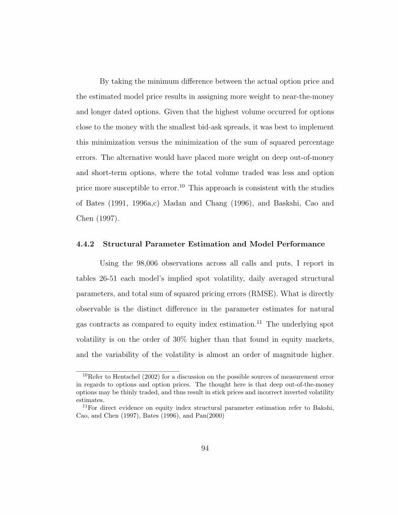
By taking the minimum difference between the actual option price and
the estimated model price results in assigning more weight to near-the-money
and longer dated options. Given that the highest volume occurred for options
close to the money with the smallest bid-ask spreads, it was best to implement
this minimization versus the minimization of the sum of squared percentage
errors. The alternative would have placed more weight on deep out-of-money
and short-term options, where the total volume traded was less and option
price more susceptible to error.10 This approach is consistent with the studies
of Bates (1991, 1996a,c) Madan and Chang (1996), and Baskshi, Cao and
Chen (1997).
4.4.2 Structural Parameter Estimation and Model Performance
Using the 98,006 observations across all calls and puts, I report in
tables 26-51 each model’s implied spot volatility, daily averaged structural
parameters, and total sum of squared pricing errors (RMSE). What is directly
observable is the distinct difference in the parameter estimates for natural
gas contracts as compared to equity index estimation.11 The underlying spot
volatility is on the order of 30% higher than that found in equity markets,
and the variability of the volatility is almost an order of magnitude higher.
10Refer to Hentschel (2002) for a discussion on the possible sources of measurement errorin regards to options and option prices. The thought here is that deep out-of-the-moneyoptions may be thinly traded, and thus result in stick prices and incorrect inverted volatilityestimates.
11For direct evidence on equity index structural parameter estimation refer to Bakshi,Cao, and Chen (1997), Bates (1996), and Pan(2000)
94
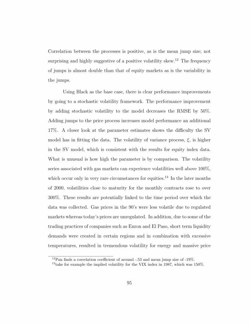
Correlation between the processes is positive, as is the mean jump size; not
surprising and highly suggestive of a positive volatility skew.12 The frequency
of jumps is almost double than that of equity markets as is the variability in
the jumps.
Using Black as the base case, there is clear performance improvements
by going to a stochastic volatility framework. The performance improvement
by adding stochastic volatility to the model decreases the RMSE by 50%.
Adding jumps to the price process increases model performance an additional
17%. A closer look at the parameter estimates shows the difficulty the SV
model has in fitting the data. The volatility of variance process, ξ, is higher
in the SV model, which is consistent with the results for equity index data.
What is unusual is how high the parameter is by comparison. The volatility
series associated with gas markets can experience volatilities well above 100%,
which occur only in very rare circumstances for equities.13 In the later months
of 2000, volatilities close to maturity for the monthly contracts rose to over
300%. These results are potentially linked to the time period over which the
data was collected. Gas prices in the 90’s were less volatile due to regulated
markets whereas today’s prices are unregulated. In addition, due to some of the
trading practices of companies such as Enron and El Paso, short term liquidity
demands were created in certain regions and in combination with excessive
temperatures, resulted in tremendous volatility for energy and massive price
12Pan finds a correlation coefficient of around -.53 and mean jump size of -19%.13take for example the implied volatility for the VIX index in 1987, which was 150%.
95
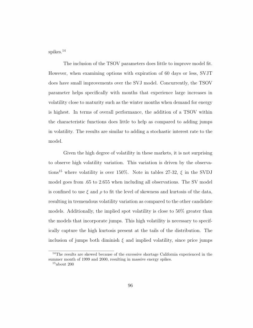
spikes.14
The inclusion of the TSOV parameters does little to improve model fit.
However, when examining options with expiration of 60 days or less, SVJT
does have small improvements over the SVJ model. Concurrently, the TSOV
parameter helps specifically with months that experience large increases in
volatility close to maturity such as the winter months when demand for energy
is highest. In terms of overall performance, the addition of a TSOV within
the characteristic functions does little to help as compared to adding jumps
in volatility. The results are similar to adding a stochastic interest rate to the
model.
Given the high degree of volatility in these markets, it is not surprising
to observe high volatility variation. This variation is driven by the observa-
tions15 where volatility is over 150%. Note in tables 27-32, ξ in the SVDJ
model goes from .65 to 2.655 when including all observations. The SV model
is confined to use ξ and ρ to fit the level of skewness and kurtosis of the data,
resulting in tremendous volatility variation as compared to the other candidate
models. Additionally, the implied spot volatility is close to 50% greater than
the models that incorporate jumps. This high volatility is necessary to specif-
ically capture the high kurtosis present at the tails of the distribution. The
inclusion of jumps both diminish ξ and implied volatility, since price jumps
14The results are skewed because of the excessive shortage California experienced in thesummer month of 1999 and 2000, resulting in massive energy spikes.
15about 200
96
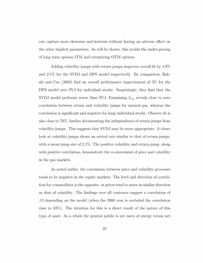
can capture more skewness and kurtosis without having an adverse effect on
the other implicit parameters. As will be shown, this avoids the under-pricing
of long term options ITM and overpricing OTM options.
Adding volatility jumps with return jumps improves overall fit by 4.9%
and 2.1% for the SVDJ and DPS model respectively. By comparison, Bak-
shi and Cao (2003) find an overall performance improvement of 3% for the
DPS model over SVJ for individual stocks. Surprisingly, they find that the
SVDJ model performs worse than SVJ. Examining δx,y reveals close to zero
correlation between return and volatility jumps for natural gas, whereas the
correlation is significant and negative for large individual stocks. Observe do is
also close to 70%, further documenting the independence of return-jumps from
volatility-jumps. This suggests that SVDJ may be more appropriate. A closer
look at volatility-jumps shows an arrival rate similar to that of return-jumps,
with a mean jump size of 2.1%. The positive volatility and return-jump, along
with positive correlation, demonstrate the co-movement of price and volatility
in the gas markets.
As noted earlier, the correlation between price and volatility processes
tends to be negative in the equity markets. The level and direction of correla-
tion for commodities is the opposite, as prices tend to move in similar direction
as that of volatility. The findings over all contracts suggest a correlation of
.15 depending on the model (when the 2000 year is excluded the correlation
rises to 33%). The intuition for this is a direct result of the nature of this
type of asset. As a whole the general public is net users of energy versus net
97
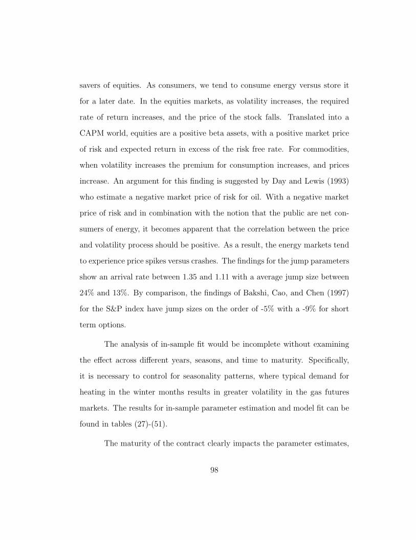
savers of equities. As consumers, we tend to consume energy versus store it
for a later date. In the equities markets, as volatility increases, the required
rate of return increases, and the price of the stock falls. Translated into a
CAPM world, equities are a positive beta assets, with a positive market price
of risk and expected return in excess of the risk free rate. For commodities,
when volatility increases the premium for consumption increases, and prices
increase. An argument for this finding is suggested by Day and Lewis (1993)
who estimate a negative market price of risk for oil. With a negative market
price of risk and in combination with the notion that the public are net con-
sumers of energy, it becomes apparent that the correlation between the price
and volatility process should be positive. As a result, the energy markets tend
to experience price spikes versus crashes. The findings for the jump parameters
show an arrival rate between 1.35 and 1.11 with a average jump size between
24% and 13%. By comparison, the findings of Bakshi, Cao, and Chen (1997)
for the S&P index have jump sizes on the order of -5% with a -9% for short
term options.
The analysis of in-sample fit would be incomplete without examining
the effect across different years, seasons, and time to maturity. Specifically,
it is necessary to control for seasonality patterns, where typical demand for
heating in the winter months results in greater volatility in the gas futures
markets. The results for in-sample parameter estimation and model fit can be
found in tables (27)-(51).
The maturity of the contract clearly impacts the parameter estimates,
98
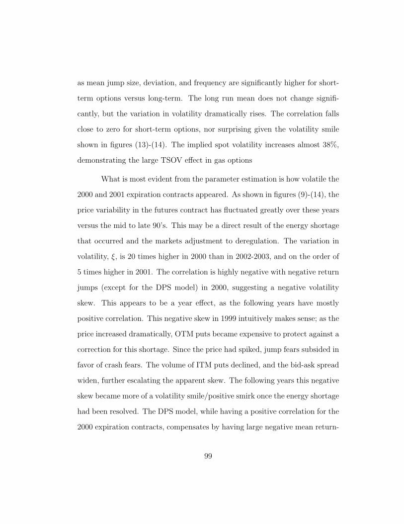
as mean jump size, deviation, and frequency are significantly higher for short-
term options versus long-term. The long run mean does not change signifi-
cantly, but the variation in volatility dramatically rises. The correlation falls
close to zero for short-term options, nor surprising given the volatility smile
shown in figures (13)-(14). The implied spot volatility increases almost 38%,
demonstrating the large TSOV effect in gas options
What is most evident from the parameter estimation is how volatile the
2000 and 2001 expiration contracts appeared. As shown in figures (9)-(14), the
price variability in the futures contract has fluctuated greatly over these years
versus the mid to late 90’s. This may be a direct result of the energy shortage
that occurred and the markets adjustment to deregulation. The variation in
volatility, ξ, is 20 times higher in 2000 than in 2002-2003, and on the order of
5 times higher in 2001. The correlation is highly negative with negative return
jumps (except for the DPS model) in 2000, suggesting a negative volatility
skew. This appears to be a year effect, as the following years have mostly
positive correlation. This negative skew in 1999 intuitively makes sense; as the
price increased dramatically, OTM puts became expensive to protect against a
correction for this shortage. Since the price had spiked, jump fears subsided in
favor of crash fears. The volume of ITM puts declined, and the bid-ask spread
widen, further escalating the apparent skew. The following years this negative
skew became more of a volatility smile/positive smirk once the energy shortage
had been resolved. The DPS model, while having a positive correlation for the
2000 expiration contracts, compensates by having large negative mean return-
99
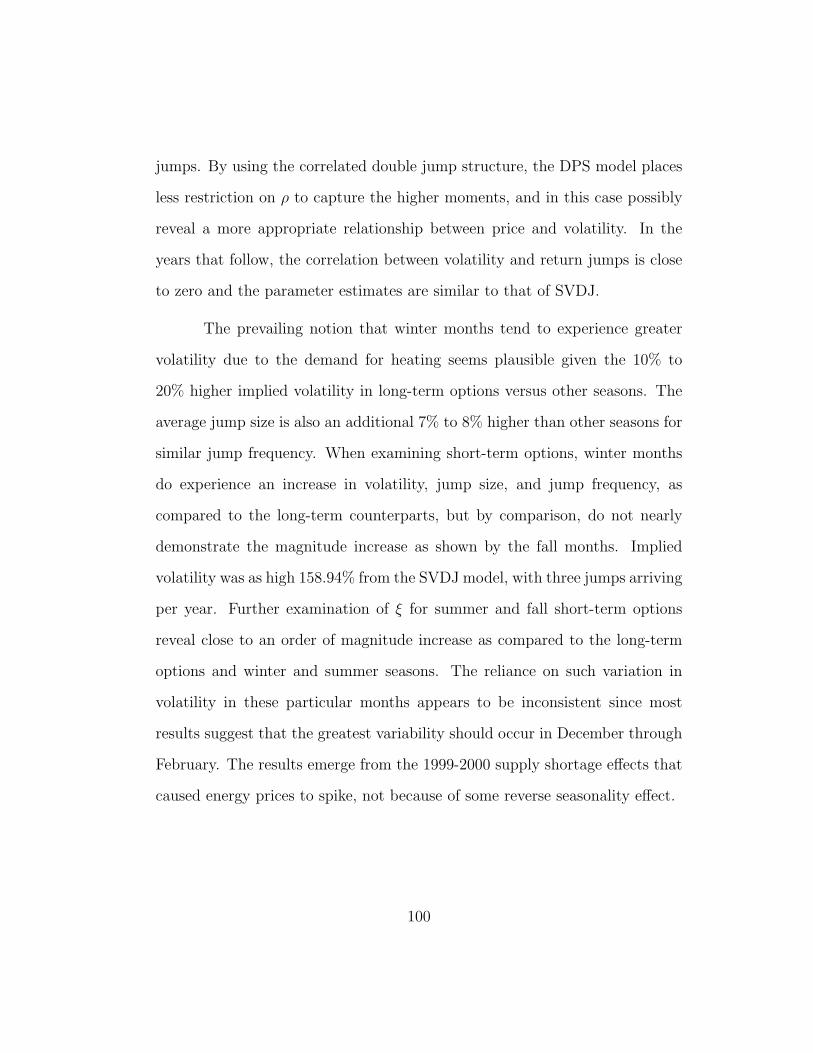
jumps. By using the correlated double jump structure, the DPS model places
less restriction on ρ to capture the higher moments, and in this case possibly
reveal a more appropriate relationship between price and volatility. In the
years that follow, the correlation between volatility and return jumps is close
to zero and the parameter estimates are similar to that of SVDJ.
The prevailing notion that winter months tend to experience greater
volatility due to the demand for heating seems plausible given the 10% to
20% higher implied volatility in long-term options versus other seasons. The
average jump size is also an additional 7% to 8% higher than other seasons for
similar jump frequency. When examining short-term options, winter months
do experience an increase in volatility, jump size, and jump frequency, as
compared to the long-term counterparts, but by comparison, do not nearly
demonstrate the magnitude increase as shown by the fall months. Implied
volatility was as high 158.94% from the SVDJ model, with three jumps arriving
per year. Further examination of ξ for summer and fall short-term options
reveal close to an order of magnitude increase as compared to the long-term
options and winter and summer seasons. The reliance on such variation in
volatility in these particular months appears to be inconsistent since most
results suggest that the greatest variability should occur in December through
February. The results emerge from the 1999-2000 supply shortage effects that
caused energy prices to spike, not because of some reverse seasonality effect.
100
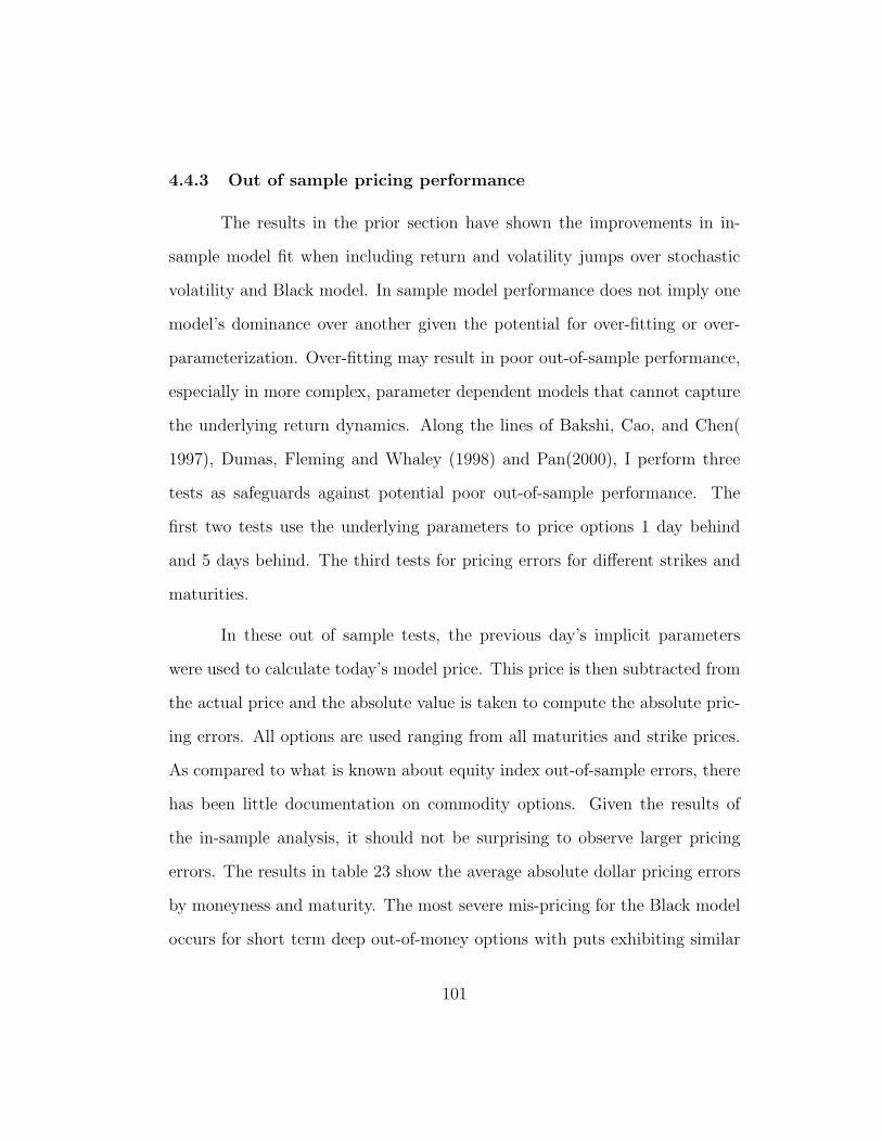
4.4.3 Out of sample pricing performance
The results in the prior section have shown the improvements in in-
sample model fit when including return and volatility jumps over stochastic
volatility and Black model. In sample model performance does not imply one
model’s dominance over another given the potential for over-fitting or over-
parameterization. Over-fitting may result in poor out-of-sample performance,
especially in more complex, parameter dependent models that cannot capture
the underlying return dynamics. Along the lines of Bakshi, Cao, and Chen(
1997), Dumas, Fleming and Whaley (1998) and Pan(2000), I perform three
tests as safeguards against potential poor out-of-sample performance. The
first two tests use the underlying parameters to price options 1 day behind
and 5 days behind. The third tests for pricing errors for different strikes and
maturities.
In these out of sample tests, the previous day’s implicit parameters
were used to calculate today’s model price. This price is then subtracted from
the actual price and the absolute value is taken to compute the absolute pric-
ing errors. All options are used ranging from all maturities and strike prices.
As compared to what is known about equity index out-of-sample errors, there
has been little documentation on commodity options. Given the results of
the in-sample analysis, it should not be surprising to observe larger pricing
errors. The results in table 23 show the average absolute dollar pricing errors
by moneyness and maturity. The most severe mis-pricing for the Black model
occurs for short term deep out-of-money options with puts exhibiting similar
101
behavior. The average dollar pricing error was $0.24, which is a significant
portion of the option price. As the option moves towards at-the-money, the
mis-pricing declines, with an average dollar pricing error of $0.04. This is the
general pattern for long-term and medium-term options, and is highly sugges-
tive of a model that is able to capture the cross-sectional dispersion in option
values. Using the Black model as a reference, the five additional models can
now be tested to show the improvements over this initial benchmark. In terms
of performance the SVDJ model shows the lowest pricing error of $0.031 for
short-term deep out-of-money calls, as compared to the $0.24 of the Black
Model. By comparison there is significant, but smaller performance improve-
ment when examining the deep out-of-money puts. This may be a function
of sample size, as there were only 17 options within this subset. Looking
at short-term ITM calls and ITM puts shows similar performance improve-
ments on order of $0.13 to $0.06. Surprisingly, the DPS model had larger
pricing errors for the deep out-of-money call options, and similar numbers to
SVDJ for the put options. The hierarchy in terms of improvement shows that
the inclusion of stochastic volatility improves upon the Black model, and the
inclusion of return-jumps further improves upon the SV model. With the in-
clusion of return jumps performance improvements are quite similar for the
SVJ, SVJT, SVDJ, and DPS models across most maturities and moneyness.
With all models, the dollar pricing errors are highest for short-term options,
deep out-of-money. The inclusion of the volatility jumps has, in some cases,
shown the ability to reduce these errors, given the model’s ability to generate
102

addition peaked implied volatility-distributions. The 5 day-ahead results do
little to change the conclusions generated from the 1 day-ahead section.
The percentage pricing errors are indicative of the moneyness/maturity
performance of each model. The errors are calculated from the sample average
of the daily difference between the model price and the actual price, divided
by the actual price. The results reveal the degree of over or under-pricing for
each model. The B model tends to under price ITM calls and over-price OTM
calls. With the inclusion of stochastic volatility, the mis-pricing is reduced, but
OTM short-term options are still overpriced by 19.07%. Adding jumps to the
model reduces the errors further, including reduced mis-pricing for longer-term
options.
4.5 Mean-Reversion in Stochastic Volatility
Estimation of the various price risk factors requires either extensive
historical data or, as shown by Pan (2000), the ability to use the both spot
prices and the cross-section of option prices. It is my intent to implement
a similar technique, using the knowledge of ex-post volatility data and the
estimated structural parameters found in the prior section. Using Monte Carlo
simulation and the closed form solutions for option prices, both the risk-neutral
and objective distributions can be combined to jointly estimate the market
price(s) of risk.
Note the minimization in equation (4.9), where the implied option
103
model volatility and structural parameters are recovered from minimizing the
difference between actual price and implied model price. These risk-neutral
parameter estimates can then be put into the model to generate option val-
ues for any moneyness/maturity combination. The option value can then be
inverted using the Black model to solve for
σ̃it, Imp = f (σ̂t, κ, ξ, θ, ρ) (4.10)
where f (·) is obtained by running the parameters κ, ξ, θ, ρ through the closed
form stochastic volatility option model16 and then inverting the option price
using the Black model. The subscript i, t denote the moneyness and time
dimension. The instantaneous volatility σ̂t is unobservable and must be es-
timated, which directly links the estimated implied volatility to the latent
factor. For each point in time and moneyness there is a corresponding ob-
servable σit,Imp, allowing for direct comparison between the model dependent
risk-neutral estimates of BIV volatility and the observable BIV. This implied
volatility comes from inverting the actual option price using the Black model.
The second equation used in estimation comes from the statistical
model analogous to the data-generating process in equations (4.1) - (4.2):
dS = (r + λSσt)S dt+ σt S dzS (4.11)
dσ2 =[κ(θ − σ2
t
)+ λσξσ
2]dt+ ξσt dzσ (4.12)
16In this example, only the stochastic volatility parameters are shown, since the initialconcern is just with the market price of volatility risk. When the other risk premium areestimated, model SVJ, SVJDJ will be used.
104
For given parameters {λS, σ̂t, κ, θ, λσ, ξ, ρ} , eqs. (4.11) - (4.12) will
produce a range of terminal values ST . The terminal values are generated
using quasi-Monte Carlo simulation, simulating the equations given in (4.11)
- (4.12)17. The Brownian motions are drawn from a N ∼ (0,√t) distribution
and the system is shocked daily. The simulation is generated 1000 times to
guarantee efficiency. From these terminal values the realized standard devia-
tion σ̃t,Realized is given by
σ̃t,Realized = g (λS, σ̂t, κ, θ, λσ, ξ, ρ) =1√T
STDEV
(lnST
S0
), (4.13)
where STDEV is the standard deviation operator
√√√√ 1
N − 1
N∑n=1
(xn − x)2
and x̄ is mean of the log daily return.
The ex-post realized volatility for that same 30-day period, to which
the RHS of equation (4.13) is set equal, is obtained from the realized-return
series over the given month
σt,Realized =
√√√√ 1
T − 1
T∑t=1
(st − s)2, (4.14)
where st = lnSt
St−1
, s ≡ 1
T
∑t
st.
Similar to the case for implied volatilities, I am able to generate real-
ized volatility dependent on the model parameters and have a actual measure
17The random draws were done using a Sobol sequence. The efficiency of estimationimproves from a standard error of 1√
nto 1
n
105
of volatility from the ex-post measure given in equation (4.13). Notice that
realized volatility is also dependent on instantaneous volatility σ̂t. By using
both the realized and implied volatility estimates, the market prices of risk
can be computed through the minimization of the difference between model
inferred volatilities and actual volatilities.
4.6 Proposed Algorithms
4.6.1 Parameter Estimation, including Market Price of Risk
The parameters I seek to solve for are {σ̂t, λs, λσ} , where λσ is the
market price of volatility risk in equation (4.12). Whereas λs and λσ are time-
invariant constants, σ̂t is the instantaneous volatility, and thus is different
from one time period to the next. For each point in time, there is an ex-post
realized volatility measure σt,Realized and Black implied volatility σt, i, Imp
from option prices over i strike prices. Using both measures of volatility, the
unknown parameters are estimated using the objective function
min{σ̂t, λs, λσ}
∑i,t
{ [f (σ̂t, κ, ξ, θ, ρ)− σt, i, Imp
]2+[g (λS, σ̂t, κ, θ, λσ, ξ, ρ)− σt,Realized
]2 }(4.15)
where f (·) is obtained via the inverted Black implied volatility from the model
dependent closed form price given in equations (4.5) - (4.7) and g (·) is obtained
106
by running a set of parameters through the simulation equations (4.11) - (4.12)
and (4.14). Eq. (4.15) may be amenable to GMM-style reformulation by noting
the covariation between f (·) and g (·) . Since there are multiple observations
of BIV for any given point in time, I minimize the difference between the
estimated realized and implied volatilities for both actual realized and implied
volatilities. This is done for each point in time, and the resulting parameters
are the average of the daily estimates from the objective function above.
The initial values for the non-linear estimation procedures are:
σt = σt, Imp
{κ, θ, ξ, ρ} = Implied parameters from SV model fit
λσ = 0
λS = 0
The estimation procedure was run on three models, SV, SVJ, and
SVDJ, to recover the market prices of risk. The return and volatility-jump
sizes were generated from the structural parameters µ, µj and σj. At each
point in time, to generate σt,Realized in the presence of jumps, the jump size
was quasi-randomly drawn from a normal distribution with the above mean
and standard deviation over the 1000 simulated paths. The arrival rates, λx
and λy, are adjusted for the market prices of jump risk, λj and λjv respectively,
such that a return-jump will arrive if,
λx(1− λj)4t ≥ B (4.16)
107
where B is drawn from a uniform∼(0,1) distribution. The correction for the
drift is given by λx(1−λj)J4t where J is the jump size drawn from the normal
N ∼ (µ, σj).
The Monte Carlo simulation is bounded such that the price and volatil-
ity cannot go below zero and the option values are calculated using the closed
form solutions specified in equations (4.5)-(4.7). The results of the minimiza-
tion of (4.15) can be found in table 52.
4.6.2 Results
For each model tested, the market price of volatility risk is negative and
significant in all cases. When controlling for return-jumps, and subsequently
for volatility-jumps, the estimate(s) for market price of volatility risk is reduced
as is the standard error of the estimate. For the gas markets, ignoring jumps
forces the underlying parameters ξ and ρ to capture the skewness and kurtosis
in the option prices, resulting in upward-biased values for these parameters.18
Since the market price of volatility risk, λσ, is linked to these underlying
values, it should be no surprise to see a much higher estimate, -17.96, than
that when return-jumps are included. Including volatility-jumps does not
change the estimate significantly from the SVJ model. The results when jumps
are included are very similar to those found in the earlier section when only
ATM implied volatilities were used in estimating the parameter. In fact, this
appeals to the intuition surrounding the dynamics of option valuation. Jumps
18refer to table 26 for parameter values.
108
are necessary to capture the behavior of the tails of the implicit distribution,
and provides better model performance in capturing the cross-section of option
prices. In the prior section, the tails were ignored, and estimates for the market
price of volatility risk for each of the months were between -8.77 and -3.46. In
this estimation, since there is a limited time-series, all months were combined,
the estimates for λσ when controlling for return jumps and return and volatility
jumps are -5.15 and -4.92 respectively. This result in particular reveals the
necessity for a having a negative market price of volatility risk to reconcile the
difference between the implied and realized distributions.
By comparison, the market price of risk, λs, is much tougher to esti-
mate due to lengthy time-series requirements to overcome significant variation
in the data. For example, in equities, if I assume λs to be .41, and the average
annual volatility is 20%, then approximately 50 years of data are needed to
arrive at significant estimates. Using the cross-section of option prices reduces
the data requirements, but as shown earlier, the volatility within the natural
gas markets is much more severe than the equities markets. The price risk
premiums found were all statistically insignificant and SVJ model suggest a
positive risk premia as compared to the SV and SVDJ models. These results
are not surprising, and lend little resolve to the ongoing debate between re-
searchers about the direction and magnitude of the market price of risk for
commodities. With the volatility observed in 1999 and 2000, it may take
several more years of data and reduced bid/ask spreads to achieve statistical
significance in either direction.
109
While not a major a concern, the results for the market price of jump
intensity risk for return and volatility-jumps show the significant premium
place on jumps in this market. To interpret the results, let us assume that a
risk-neutral jump arrives at a rate of 1 per year. If we take the SVJ model as
given, then a realized jump arrives at a rate of approximately 1 per every 2
years. For the SVDJ model, a realized return-jump arrives at 73% of the rate
of an implied return-jump. For volatilities jumps, the realized arrival rate is
51% of the implied arrival rate. This helps explain the significant skew/smile
observed in the cross-section of option prices. Consumers are concerned about
price spikes/jumps, and are willing to pay large premiums to hedge themselves
against large upturns/downturns in the market. As compared to equities, this
lends justification to why ITM and OTM options are expensive relative to
ATM options.
4.7 Conclusion
While not a surprise, natural gas implied risk-neutral parameters show
little similarity as compared to their equity counterparts. The correlation
between the processes is positive, there is positive mean jump size, and the
variation of volatility is almost 5 times higher. Using the latest additions
to the option modeling framework, the findings here suggest that an option
model that incorporates independent volatility and return-jumps is best able
to capture the cross-sectional and time-series dynamics of option prices. Incor-
porating a TSOV component had little effect on improving model performance,
110

but had a statistically significant impact on options that were close to expi-
ration. Given the significant and observable TSOV in natural gas contracts,
the results for model fit may seem unexpected, but the estimation procedure
minimized over the cross-section of daily option prices versus the time series,
reducing the potential impact of the TSOV parameter. Examining the season-
ality and yearly effects demonstrated the potential implications a cold winter,
hot summer, or energy crisis had on the parameters. Clearly, these effects were
magnified in the 1999, 2000 prices, where volatility variation was almost an
order of magnitude higher.
Through the minimization of equation (4.15), the market price of volatil-
ity risk was found to be highly negative and significant. These results were
very similar to those found through the calibration technique in section 3.3.
This premium is tied directly to the variation in volatility, which is signifi-
cantly higher than that found for equities. Selling options is a way to capture
the premium, as investors are willing to hedge against volatility variation by
either buying puts or calls. This protection is expensive, and as shown by
Eraker (2001), leads to equity Sharpe ratios six times that found for trading
equities. These ratios are close to 10 times that found for equities, but the nat-
ural gas markets are almost twice as volatile, and protection against volatility
change will ultimately be more expensive. Disappointingly, pinning down a
market price of risk for natural gas proved fruitless, as the degree of volatility
in the market and length of the data prevented significant estimates. However,
using this technique will further researchers’ efforts in future, due to market
111

stabilization and the availability of more usable data. Hopefully, solving the
magnitude and direction of the market price of risk is just observations away.
As for the main goal of this work, establishing a significant and negative
market price of volatility risk, all results clearly indicate the degree to which
this premium matters in the market. Through relating the bias in Black-
Scholes/Black implied volatility to realized-term volatility, to the estimation
of risk-neutral structural parameters, all findings suggest a negative volatility
risk premium. Understanding how investors place premiums on volatility helps
to solve phenomena such as the volatility smile/skew in the cross-section of
option prices, the reason why option traders like to be short, and why implied
volatility is upward bias predictor of future realized-term volatility.
112

Tables and Figures
113
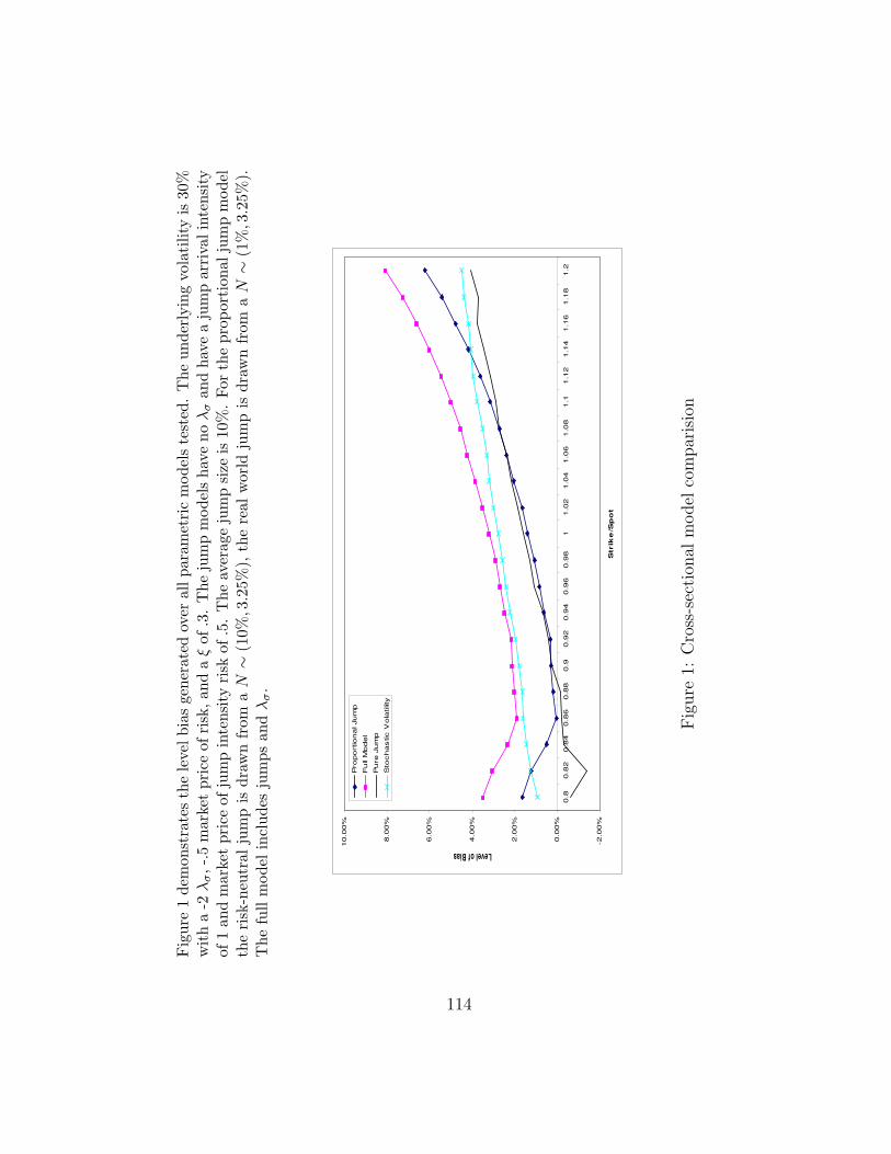
Fig
ure
1de
mon
stra
tes
the
leve
lbia
sge
nera
ted
over
allp
aram
etri
cm
odel
ste
sted
.T
heun
derl
ying
vola
tilit
yis
30%
wit
ha
-2λ
σ,-
.5m
arke
tpr
ice
ofri
sk,a
nda
ξof
.3.
The
jum
pm
odel
sha
veno
λσ
and
have
aju
mp
arri
vali
nten
sity
of1
and
mar
ket
pric
eof
jum
pin
tens
ity
risk
of.5
.T
heav
erag
eju
mp
size
is10
%.
For
the
prop
orti
onal
jum
pm
odel
the
risk
-neu
tral
jum
pis
draw
nfr
oma
N∼
(10%
,3.2
5%),
the
real
wor
ldju
mp
isdr
awn
from
aN∼
(1%
,3.2
5%).
The
full
mod
elin
clud
esju
mps
and
λσ.
-2.0
0%
0.0
0%
2.0
0%
4.0
0%
6.0
0%
8.0
0%
10.0
0%
0.8
0.8
20.8
40.8
60.8
80.9
0.9
20.9
40.9
60.9
81
1.0
21.0
41.0
61.0
81.1
1.1
21.1
41.1
61.1
81.2
Str
ike
/Sp
ot
Level of Bias
Pro
port
ional Jum
p
Full
Model
Pure
Jum
p
Sto
chastic V
ola
tilit
y
Fig
ure
1:C
ross
-sec
tion
alm
odel
com
par
isio
n
114
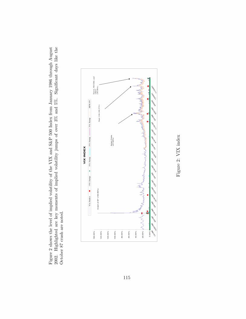
Fig
ure
2sh
ows
the
leve
lof
impl
ied
vola
tilit
yof
the
VIX
and
S&P
500
Inde
xfr
omJa
nuar
y19
86th
roug
hA
ugus
t20
02.
Hig
hlig
hted
are
key
mom
ents
ofim
plie
dvo
lati
lity
jum
psof
over
3%an
d5%
.Si
gnifi
cant
days
like
the
Oct
ober
87cr
ash
are
note
d.
VIX
IN
DE
X
0.0
0%
20.0
0%
40.0
0%
60.0
0%
80.0
0%
100.0
0%
120.0
0%
140.0
0%
160.0
0%
1/3/
1986
10/2
0/19
868/
5/19
875/
19/1
988
3/6/
1989
12/1
8/19
8910
/3/1
990
7/22
/199
15/
6/19
922/
19/1
993
12/3
/199
39/
20/1
994
7/6/
1995
4/19
/199
62/
4/19
9711
/18/
1997
9/4/
1998
6/23
/199
94/
6/20
001/
23/2
001 11
/12/
2001
Vix
Ind
ex
-5%
Jum
p5
% J
um
p-3
% J
um
p3
% J
um
pS
PX
IV
Cra
sh o
f 87' (1
50.9
0%
)
Asia
n C
risis
(4
7.5
2%
)
Sep
t 1
1th
(4
8.2
7%
)
Enro
n,
WC
OM
, and
oth
ers
(50
.48
%)
Fig
ure
2:V
IXin
dex
115
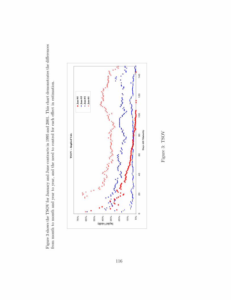
Fig
ure
3sh
owsth
eT
SOV
forJa
nuar
yan
dJu
neco
ntra
ctsin
1995
and
2001
.T
hisch
artde
mon
stra
testh
edi
ffere
nces
from
mon
thto
mon
than
dye
arto
year
,an
dth
ene
edto
cont
rolfo
rea
cheff
ect
ines
tim
atio
n.
TS
OV
--
Impl
ied
Vol
s
5%
15
%
25
%
35
%
45
%
55
%
65
%
75
%
02
04
06
08
01
00
12
01
40
Day
s ti
ll M
atu
rity
Implied VolatilityJ
an-9
5J
un
-95
Ju
n-0
1J
an-0
1
Fig
ure
3:T
SO
V
116
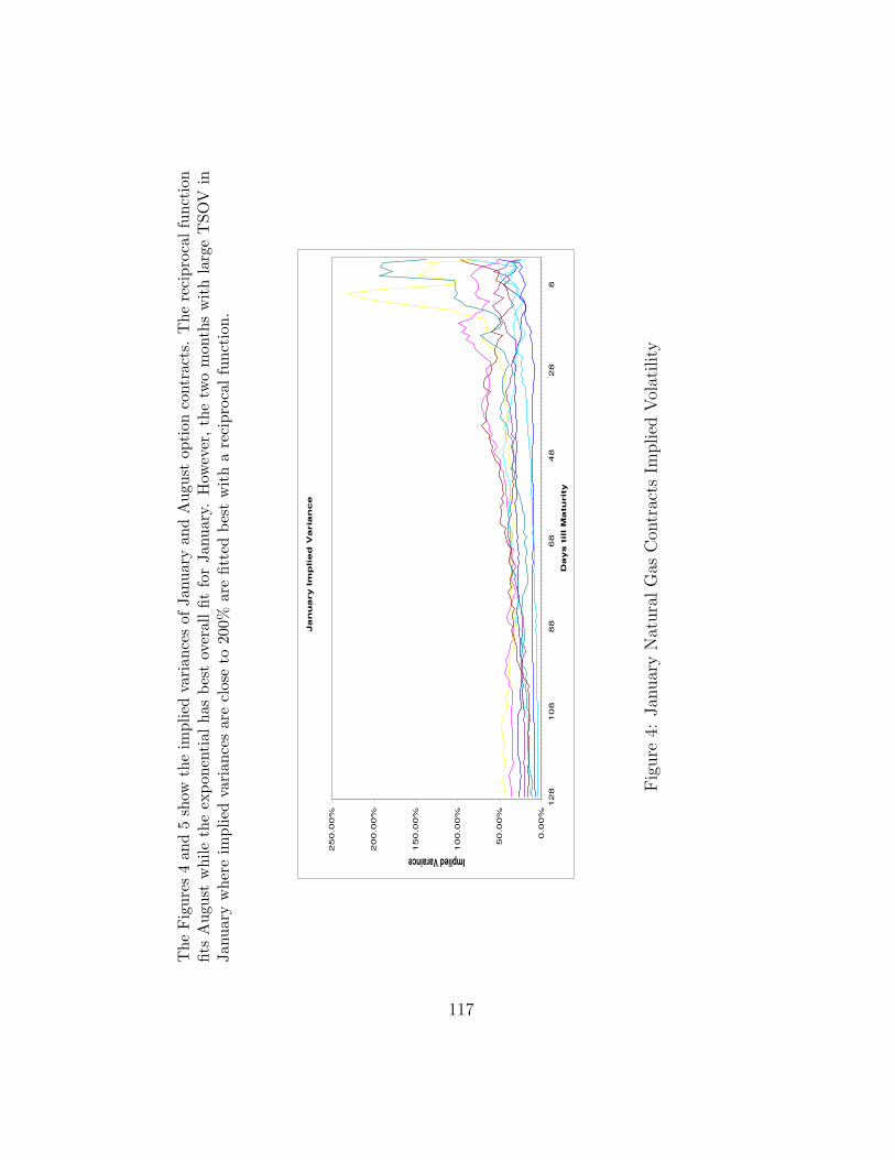
The
Fig
ures
4an
d5
show
the
impl
ied
vari
ance
sof
Janu
ary
and
Aug
ust
opti
onco
ntra
cts.
The
reci
proc
alfu
ncti
onfit
sA
ugus
tw
hile
the
expo
nent
ialha
sbe
stov
eral
lfit
for
Janu
ary.
How
ever
,th
etw
om
onth
sw
ith
larg
eT
SOV
inJa
nuar
yw
here
impl
ied
vari
ance
sar
ecl
ose
to20
0%ar
efit
ted
best
wit
ha
reci
proc
alfu
ncti
on.
Ja
nu
ary
Im
pli
ed
Va
ria
nc
e
0.0
0%
50
.00
%
10
0.0
0%
15
0.0
0%
20
0.0
0%
25
0.0
0%
12
81
08
88
68
48
28
8
Da
ys
till M
atu
rity
Implied Varaince
Fig
ure
4:Jan
uar
yN
atura
lG
asC
ontr
acts
Implied
Vol
atility
117
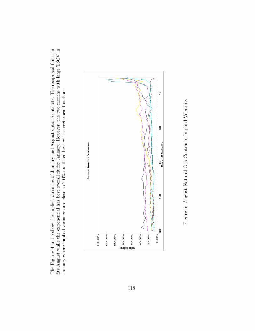
The
Fig
ures
4an
d5
show
the
impl
ied
vari
ance
sof
Janu
ary
and
Aug
ust
opti
onco
ntra
cts.
The
reci
proc
alfu
ncti
onfit
sA
ugus
tw
hile
the
expo
nent
ialha
sbe
stov
eral
lfit
for
Janu
ary.
How
ever
,th
etw
om
onth
sw
ith
larg
eT
SOV
inJa
nuar
yw
here
impl
ied
vari
ance
sar
ecl
ose
to20
0%ar
efit
ted
best
wit
ha
reci
proc
alfu
ncti
on.
Au
gu
st
Imp
lie
d V
ari
an
ce
0.0
0%
20
.00
%
40
.00
%
60
.00
%
80
.00
%
10
0.0
0%
12
0.0
0%
14
0.0
0%
12
81
08
88
68
48
Da
ys
till M
atu
rity
Implied Variance
Fig
ure
5:A
ugu
stN
atura
lG
asC
ontr
acts
Implied
Vol
atility
118
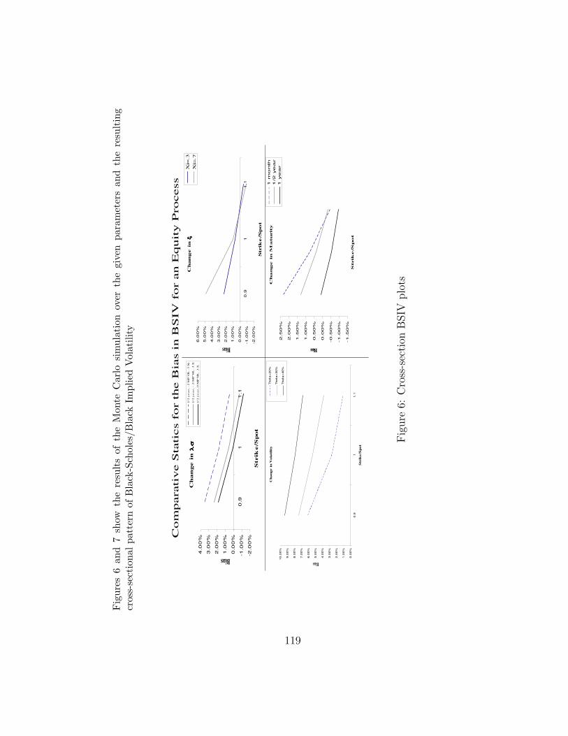
Fig
ures
6an
d7
show
the
resu
lts
ofth
eM
onte
Car
losi
mul
atio
nov
erth
egi
ven
para
met
ers
and
the
resu
ltin
gcr
oss-
sect
iona
lpa
tter
nof
Bla
ck-S
chol
es/B
lack
Impl
ied
Vol
atili
ty
Co
mpara
tive S
tati
cs
for
the B
ias i
n B
SIV
for
an E
quit
y P
rocess
Ch
an
ge
in
Vo
lati
lity
0.0
0%
1.0
0%
2.0
0%
3.0
0%
4.0
0%
5.0
0%
6.0
0%
7.0
0%
8.0
0%
9.0
0%
10.0
0%
0.9
11.1
Str
ike
/Sp
ot
Bias
Theta
=20%
Theta
=30%
Theta
=40%
Cha
ng
e i
n M
atu
rit
y
-1.5
0%
-1.0
0%
-0.5
0%
0.0
0%
0.5
0%
1.0
0%
1.5
0%
2.0
0%
2.5
0%
Strik
e/S
pot
Bias
1 m
onth
1/2
ye
ar
1 y
ea
r
Ch
an
ge
in
ξ ξξξ
-2.0
0%
-1.0
0%
0.0
0%
1.0
0%
2.0
0%
3.0
0%
4.0
0%
5.0
0%
6.0
0%
0.9
11
.1
Str
ike
/Sp
ot
Bias
Xi=
.3
Xi=
.7C
ha
ng
e i
n λ
σλ
σλ
σλ
σ
-2.0
0%
-1.0
0%
0.0
0%
1.0
0%
2.0
0%
3.0
0%
4.0
0%
0.9
11
.1
Str
ike/S
pot
Bias1/2
ye
ar, -2
MP
VR
, .3
Xi
1/2
ye
ar, -.5
MP
VR
, .3
X
1/2
ye
ar, 0
MP
VR
, .3
X
Fig
ure
6:C
ross
-sec
tion
BSIV
plo
ts
119
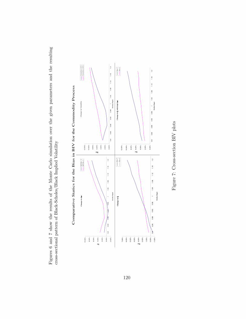
Fig
ures
6an
d7
show
the
resu
lts
ofth
eM
onte
Car
losi
mul
atio
nov
erth
egi
ven
para
met
ers
and
the
resu
ltin
gcr
oss-
sect
iona
lpa
tter
nof
Bla
ck-S
chol
es/B
lack
Impl
ied
Vol
atili
ty
Ch
ange
in
ξ
ξ ξ
ξ w
ith
hig
h λ
σ λ
σ λ
σ λ
σ
0.0
0%
2.0
0%
4.0
0%
6.0
0%
8.0
0%
10.0
0%
12.0
0%
0.8
0.8
40.8
80.9
20.9
61
1.0
41.0
81.1
21.1
61.2
Str
ike
/Sp
ot
Bias
Xi=
.7
Xi=
.3
Co
mp
ara
tiv
e S
tati
cs
for
the B
ias
in B
IVfo
r th
e C
om
mo
dit
y P
rocess
Ch
an
ge i
n λ
σλ
σλ
σλ
σ
-2.0
0%
0.0
0%
2.0
0%
4.0
0%
6.0
0%
8.0
0%
10.0
0%
0.8
0.8
40.8
80.9
20.9
61
1.0
41.0
81.1
21.1
61.2
Str
ike
/Sp
ot
Bias
MP
VR
=-.
5
MP
VR
=-2
Ch
an
ge
in
Vo
lati
lity
0.0
0%
2.0
0%
4.0
0%
6.0
0%
8.0
0%
10.0
0%
12.0
0%
0.8
0.8
40.8
80.9
20.9
61
1.0
41.0
81.1
21.1
61.2
Str
ike
/Sp
ot
Bias
Vo
lati
lity
=2
0%
Vo
lati
lity
=4
0%
Cha
nge
in ξ ξξξ
-1.0
0%
0.0
0%
1.0
0%
2.0
0%
3.0
0%
4.0
0%
5.0
0%
6.0
0%
7.0
0%
0.8
0.8
40.8
80.9
20.9
61
1.0
41.0
81.1
21.1
61.2
Str
ike
/Sp
ot
Bias
Xi=
.7
Xi=
.3
Fig
ure
7:C
ross
-sec
tion
BIV
plo
ts
120
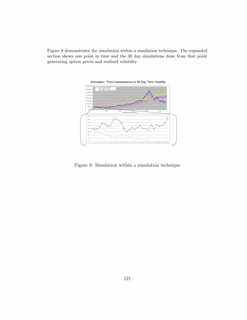
Figure 8 demonstrates the simulation within a simulation technique. The expandedsection shows one point in time and the 30 day simulations done from that pointgenerating option prices and realized volatility.
$0.00
$50.00
$100.00
$150.00
$200.00
$250.00
$300.00
$350.00
$400.00
1 365 729 1093 1457 1821
Days since inception
"price with-.5 mpvr"
price with no mpvr
Price with -2 mpvr and .5 Xi
Simulation: From Instantaneous to 30-Day Term Volatility
46
47
48
49
50
51
52
53
54
1 2 3 4 5 6 7 8 9 10 11 12 13 14 15 16 17 18 19 20 21 22 23 24 25 26 27 28 29
Figure 8: Simulation within a simulation technique
121
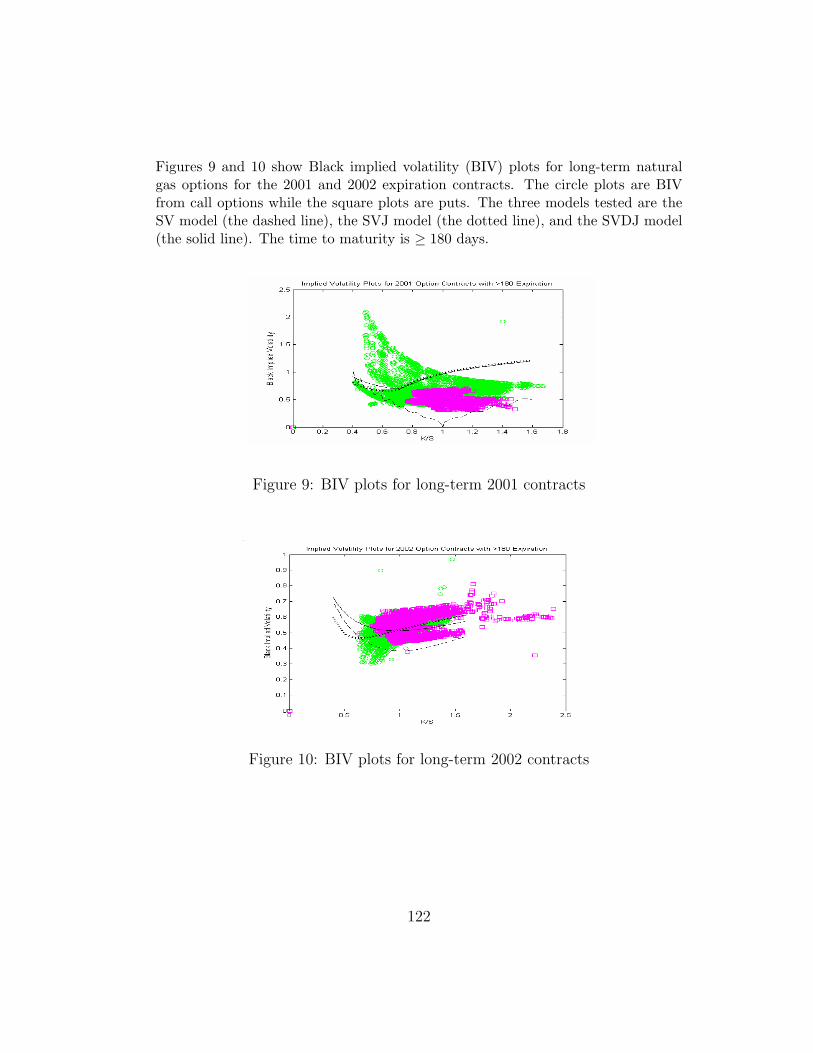
Figures 9 and 10 show Black implied volatility (BIV) plots for long-term naturalgas options for the 2001 and 2002 expiration contracts. The circle plots are BIVfrom call options while the square plots are puts. The three models tested are theSV model (the dashed line), the SVJ model (the dotted line), and the SVDJ model(the solid line). The time to maturity is ≥ 180 days.
Figure 9: BIV plots for long-term 2001 contracts
Figure 10: BIV plots for long-term 2002 contracts
122
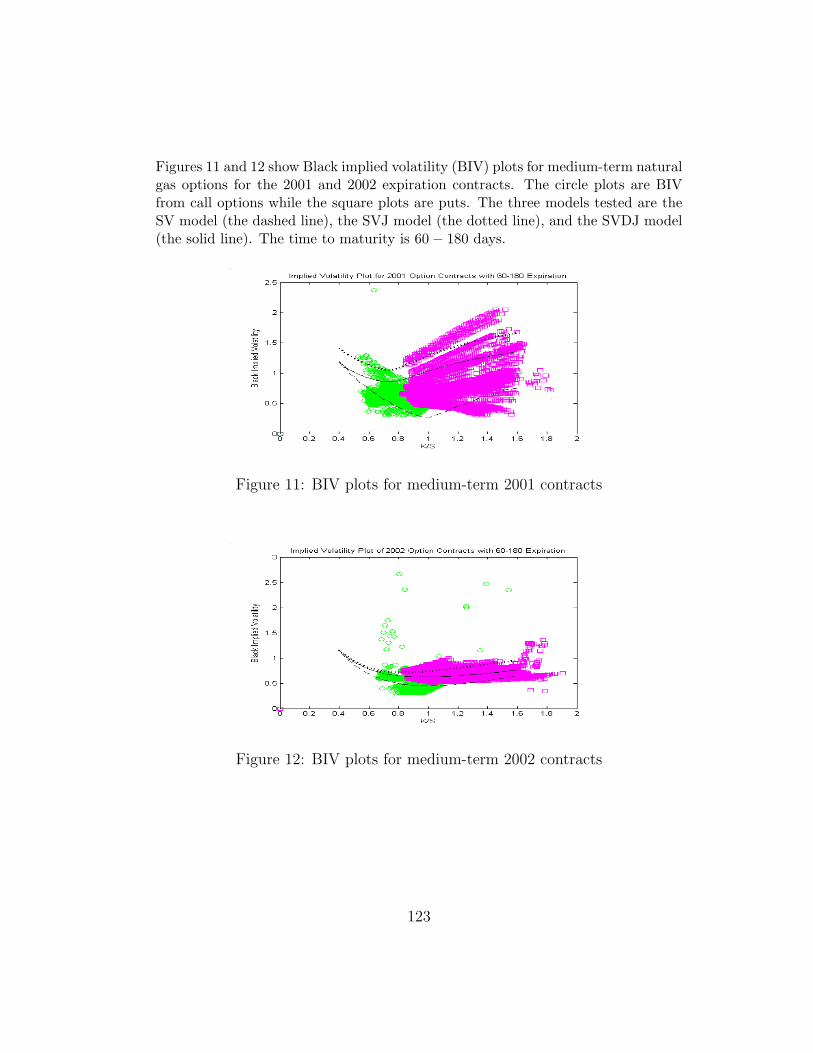
Figures 11 and 12 show Black implied volatility (BIV) plots for medium-term naturalgas options for the 2001 and 2002 expiration contracts. The circle plots are BIVfrom call options while the square plots are puts. The three models tested are theSV model (the dashed line), the SVJ model (the dotted line), and the SVDJ model(the solid line). The time to maturity is 60− 180 days.
Figure 11: BIV plots for medium-term 2001 contracts
Figure 12: BIV plots for medium-term 2002 contracts
123
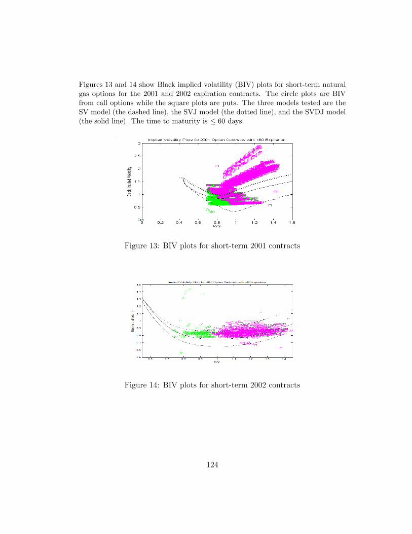
Figures 13 and 14 show Black implied volatility (BIV) plots for short-term naturalgas options for the 2001 and 2002 expiration contracts. The circle plots are BIVfrom call options while the square plots are puts. The three models tested are theSV model (the dashed line), the SVJ model (the dotted line), and the SVDJ model(the solid line). The time to maturity is ≤ 60 days.
Figure 13: BIV plots for short-term 2001 contracts
Figure 14: BIV plots for short-term 2002 contracts
124
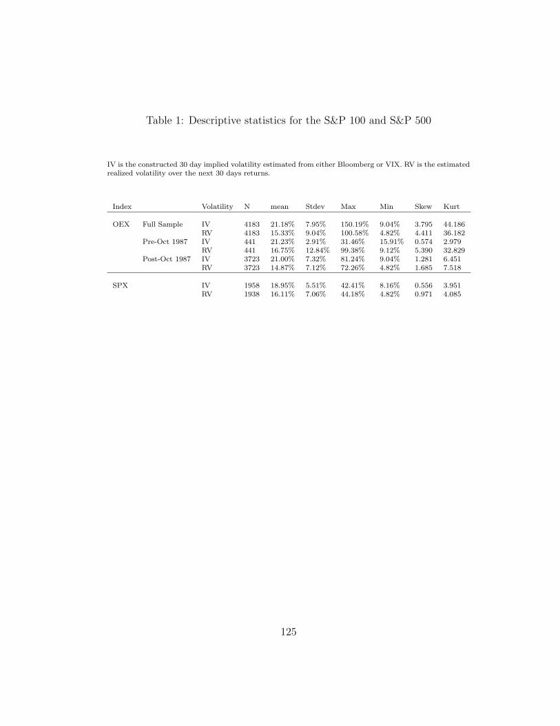
Table 1: Descriptive statistics for the S&P 100 and S&P 500
IV is the constructed 30 day implied volatility estimated from either Bloomberg or VIX. RV is the estimatedrealized volatility over the next 30 days returns.
Index Volatility N mean Stdev Max Min Skew Kurt
OEX Full Sample IV 4183 21.18% 7.95% 150.19% 9.04% 3.795 44.186RV 4183 15.33% 9.04% 100.58% 4.82% 4.411 36.182
Pre-Oct 1987 IV 441 21.23% 2.91% 31.46% 15.91% 0.574 2.979RV 441 16.75% 12.84% 99.38% 9.12% 5.390 32.829
Post-Oct 1987 IV 3723 21.00% 7.32% 81.24% 9.04% 1.281 6.451RV 3723 14.87% 7.12% 72.26% 4.82% 1.685 7.518
SPX IV 1958 18.95% 5.51% 42.41% 8.16% 0.556 3.951RV 1938 16.11% 7.06% 44.18% 4.82% 0.971 4.085
125

Tab
le2:
Gas
Con
trac
ts
Des
crip
tive
statist
ics
ofdaily
retu
rns
for
natu
ralgas
futu
res
contr
act
s
Jan
Feb
Mar
Apr
May
Jun
Jul
Aug
Sep
Oct
Nov
Dec
Aver
age
0.0
435%
0.0
238%
0.0
327%
0.0
451%
0.0
582%
0.0
552%
0.0
578%
0.0
444%
0.0
478%
0.0
488%
0.0
481%
0.0
41%
Std
ev25.9
0%
27.9
3%
27.3
7%
25.7
4%
24.7
8%
24.4
9%
24.6
7%
24.7
5%
25.6
3%
26.5
8%
25.0
9%
24.3
1%
Max
15.9
9%
17.0
6%
14.7
1%
10.2
8%
10.0
6%
9.7
3%
9.4
6%
10.3
0%
12.0
8%
11.6
4%
11.1
8%
11.0
1%
Min
-13.4
7%
-14.7
3%
-15.3
7%
-10.7
0%
-7.9
9%
-7.8
4%
-9.4
6%
-9.0
8%
-10.0
4%
-10.7
0%
-8.7
1%
-10.0
3%
Skew
0.2
5-0
.06
-0.1
6-0
.02
0.0
90.0
20.0
10.0
10.0
50.0
70.1
3-0
.06
Kurt
9.4
811.3
67.9
84.2
63.8
83.8
64.1
14.3
14.6
94.9
34.9
05.3
6
126

Table 3: Number of days with greater than 5% price movementsYear Jan Feb Mar Apr May Jun Jul Aug Sep Oct Nov Dec Total1991 0 0 1 1 1 1 1 1 3 2 0 0 111992 0 0 2 2 3 1 2 2 2 4 2 1 211993 0 2 0 4 4 0 0 0 0 0 0 0 101994 1 3 3 0 0 0 0 0 0 0 0 0 71995 2 2 1 2 1 1 1 0 1 1 1 0 131996 4 6 10 4 1 0 0 1 2 3 6 9 461997 9 11 6 6 6 1 1 1 2 N/A 7 5 551998 2 1 1 1 2 0 2 2 3 9 5 3 311999 4 4 1 2 1 0 0 2 2 4 2 3 252000 4 4 3 0 0 2 4 4 8 6 7 10 522001 15 13 15 10 8 8 9 8 7 8 12 11 1242002 13 14 12 15 16 17 19 15 18 17 12 7 1752003 4 4 5 8 8 8 6 4 4 4 4 3 622004 3 1 1 2 2 1 1 1 1 0 0 0 132005 0 0 0 0 0 0 0 0 0 0 0 0 02006 0 0 0 0 0 0 0 0 0 0 0 N/A 02007 0 0 0 0 0 0 0 0 0 N/A N/A N/A 0Total 61 65 61 57 53 40 46 41 53 58 58 52 645
Table 4: Number of days with greater than 10% price movementsJan Feb Mar Apr May Jun Jul Aug Sep Oct Nov Dec Total
5 9 6 1 1 0 0 1 1 2 2 1 29
127
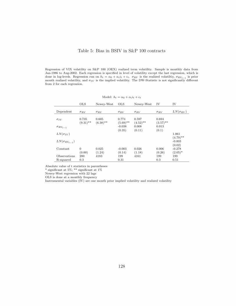
Table 5: Bias in BSIV in S&P 100 contracts
Regression of VIX volatility on S&P 100 (OEX) realized term volatility. Sample is monthly data fromJan-1986 to Aug-2002. Each regression is specified in level of volatility except the last regression, which isdone in log-levels. Regression run on ht = α0 + αiit + εt. σRV is the realized volatiltiy, σRVt−1 is priormonth realized volatility, and σIV is the implied volatility. The DW-Statistic is not significantly differentfrom 2 for each regression.
Model: ht = α0 + αiit + εt
OLS Newey-West OLS Newey-West IV IV
Dependent σRV σRV σRV σRV σRV LN(σRV )
σIV 0.735 0.605 0.774 0.597 0.694(9.31)** (6.38)** (5.69)** (4.52)** (3.57)**
σRVt−1 -0.038 0.008 0.013
(0.35) (0.11) (0.1)LN(σIV ) 1.061
(4.79)**LN(σRVt−1 ) -0.003
(0.02)Constant 0 0.025 -0.003 0.026 0.006 -0.278
(0.00) (1.24) (0.14) (1.18) (0.26) (2.05)*Observations 200 4183 199 4161 199 199R-squared 0.3 0.31 0.3 0.51
Absolute value of t statistics in parentheses* significant at 5%; ** significant at 1%Newey-West regression with 22 lagsOLS is done at a monthly frequencyInstrumental variables (IV) are one month prior implied volatility and realized volatility
128
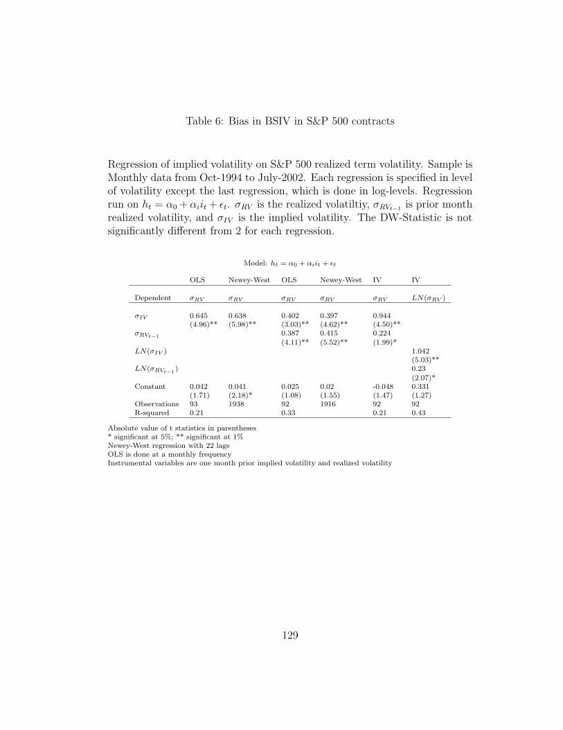
Table 6: Bias in BSIV in S&P 500 contracts
Regression of implied volatility on S&P 500 realized term volatility. Sample isMonthly data from Oct-1994 to July-2002. Each regression is specified in levelof volatility except the last regression, which is done in log-levels. Regressionrun on ht = α0 + αiit + εt. σRV is the realized volatiltiy, σRVt−1 is prior monthrealized volatility, and σIV is the implied volatility. The DW-Statistic is notsignificantly different from 2 for each regression.
Model: ht = α0 + αiit + εt
OLS Newey-West OLS Newey-West IV IV
Dependent σRV σRV σRV σRV σRV LN(σRV )
σIV 0.645 0.638 0.402 0.397 0.944(4.96)** (5.98)** (3.03)** (4.62)** (4.50)**
σRVt−1 0.387 0.415 0.224
(4.11)** (5.52)** (1.99)*LN(σIV ) 1.042
(5.03)**LN(σRVt−1 ) 0.23
(2.07)*Constant 0.042 0.041 0.025 0.02 -0.048 0.331
(1.71) (2.18)* (1.08) (1.55) (1.47) (1.27)Observations 93 1938 92 1916 92 92R-squared 0.21 0.33 0.21 0.43
Absolute value of t statistics in parentheses* significant at 5%; ** significant at 1%Newey-West regression with 22 lagsOLS is done at a monthly frequencyInstrumental variables are one month prior implied volatility and realized volatility
129
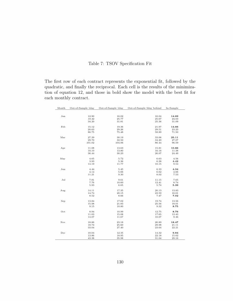
Table 7: TSOV Specification Fit
The first row of each contract represents the exponential fit, followed by thequadratic, and finally the reciprocal. Each cell is the results of the minimiza-tion of equation 12, and those in bold show the model with the best fit foreach monthly contract.
Month Out-of-Sample 1day Out-of-Sample 1day Out-of-Sample 5day behind In-Sample
Jan 12.90 16.02 16.04 14.6919.42 25.77 25.67 24.0334.20 31.81 25.36 31.09
Feb 15.12 19.36 21.97 14.6620.63 29.26 29.51 23.2386.75 75.48 58.89 71.50
Mar 27.39 30.19 33.06 25.1129.70 32.50 34.20 27.07
101.02 104.06 86.44 96.59
Apr 11.08 13.63 15.81 10.8610.10 13.80 16.16 11.3836.44 30.23 26.07 24.49
May 4.65 5.72 6.63 4.563.93 5.36 6.28 4.42
14.19 11.77 10.15 9.54
Jun 4.44 5.45 6.33 4.344.14 5.66 6.62 4.66
11.21 9.30 8.02 7.53
Jul 7.81 9.61 11.15 7.657.76 10.60 12.41 8.745.93 6.65 5.74 5.39
Aug 14.11 17.35 20.13 13.8314.74 20.15 23.59 16.618.52 8.66 7.47 7.02
Sep 13.84 17.02 19.74 13.5615.98 21.83 25.56 18.019.15 10.80 9.32 8.75
Oct 8.94 10.99 12.75 8.7611.03 15.08 17.65 12.4314.07 11.67 10.07 9.46
Nov 18.86 23.18 26.89 18.4718.74 25.60 29.98 21.1133.04 27.40 23.64 22.21
Dec 10.04 12.35 14.32 9.8413.86 18.95 22.18 15.6243.38 35.98 31.04 29.16
130
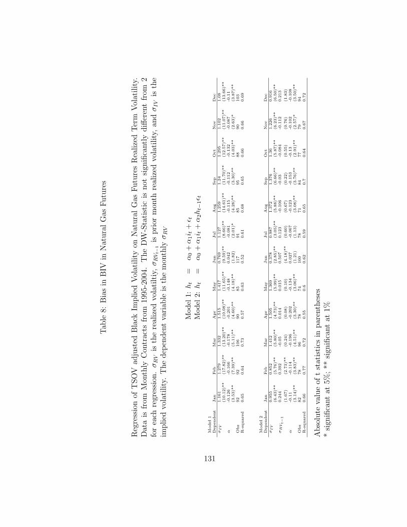
Tab
le8:
Bia
sin
BIV
inN
atura
lG
asFutu
res
Reg
ress
ion
ofT
SO
Vad
just
edB
lack
Implied
Vol
atility
onN
atura
lG
asFutu
res
Rea
lize
dTer
mV
olat
ility.
Dat
ais
from
Mon
thly
Con
trac
tsfr
om19
95-2
004.
The
DW
-Sta
tist
icis
not
sign
ifica
ntl
ydiff
eren
tfr
om2
for
each
regr
essi
on.σ
RV
isth
ere
aliz
edvo
lati
ltiy
,σ
RV
t−1
isprior
mon
thre
aliz
edvo
lati
lity
,an
dσ
IV
isth
eim
plied
vola
tility
.T
he
dep
enden
tva
riab
leis
the
mon
thlyσ
RV
Mod
el1:
ht
=α
0+
α1i t
+ε t
Mod
el2:
ht
=α
0+
α1i t
+α
2h
t−1ε t
Model1
Dependent
Jan
Feb
Mar
Apr
May
Jun
Jul
Aug
Sep
Oct
Nov
Dec
σI
V1.1
61
1.2
79
1.3
32
1.5
15
1.4
17
0.7
69
1.1
27
1.2
59
1.2
41.2
95
1.1
02
1.0
8(1
0.1
2)*
*(1
7.8
2)*
*(1
3.2
0)*
*(1
0.0
8)*
*(1
1.6
5)*
*(9
.59)*
*(8
.66)*
*(1
4.6
1)*
*(1
1.7
0)*
*(1
2.5
7)*
*(1
1.0
7)*
*(1
3.6
6)*
*α
-0.1
26
-0.1
66
-0.1
78
-0.2
01
-0.1
48
0.0
42
-0.0
81
-0.1
15
-0.1
12
-0.1
32
-0.0
87
-0.1
1(3
.53)*
*(7
.39)*
*(5
.11)*
*(4
.60)*
*(4
.18)*
*(1
.82)
(2.0
1)*
(4.2
8)*
*(3
.30)*
*(4
.03)*
*(2
.63)*
(3.8
7)*
*O
bs
92
92
106
90
85
117
91
85
95
88
90
103
R-s
quare
d0.6
50.6
40.7
30.5
70.6
30.5
20.6
10.6
80.6
50.6
60.6
60.6
9
Model2
Dependent
Jan
Feb
Mar
Apr
May
Jun
Jul
Aug
Sep
Oct
Nov
Dec
σI
V0.9
55
0.8
52
1.4
12
1.5
05
1.3
69
0.3
78
0.9
87
1.3
72
1.3
76
1.3
61.2
26
0.9
16
(6.4
3)*
*(5
.76)*
*(5
.80)*
*(4
.73)*
*(5
.99)*
*(2
.85)*
*(3
.05)*
*(5
.88)*
*(6
.66)*
*(5
.87)*
*(6
.23)*
*(6
.50)*
*σ
RV
t−
10.2
44
0.3
92
-0.0
50.0
14
0.0
15
0.5
07
0.1
23
-0.1
06
-0.0
3-0
.084
-0.1
12
0.2
13
(1.6
7)
(2.7
3)*
*(0
.24)
(0.0
8)
(0.1
0)
(4.1
8)*
*(0
.60)
(0.6
7)
(0.2
2)
(0.5
5)
(0.7
6)
(1.8
3)
α-0
.11
-0.1
14
-0.1
96
-0.2
02
-0.1
34
0.0
27
-0.0
67
-0.1
23
-0.1
53
-0.1
3-0
.102
-0.1
08
(3.1
4)*
*(3
.83)*
*(4
.51)*
*(3
.30)*
*(3
.06)*
*(1
.21)
(1.1
3)
(3.0
8)*
*(3
.76)*
*(2
.91)*
*(2
.57)*
(3.5
0)*
*O
bs
82
78
96
78
74
100
78
71
84
77
79
94
R-s
quare
d0.6
60.7
70.7
20.5
50.6
0.6
20.5
90.6
50.7
0.6
40.6
70.7
2
Abso
lute
valu
eof
tst
atis
tics
inpar
enth
eses
*si
gnifi
cant
at5%
;**
sign
ifica
nt
at1%
131

Table 9: Perfect and Zero Correlation Case
Table below shows the degree of bias in BSIV/BIV of the extreme cases of perfect and zero correlationbetween the price and volatility process. Panel A shows the perfect correlation case and Panel B the zerocorrelation case. For the gas process the correlation is positive and the market price of risk is -.5; for theequity process it is negative and the market price of risk is .41. κ (mean reversion) and ξ (volatility of thevolatility process) are 7 and .3 for both simulations.
Equity Panel A Panel Bλσ=.41 λσ=0 λσ=.41
θ=15% θ=20% θ=30% θ=15% θ=20% θ=30% θ=15% θ=20% θ=30%K/S K/S0.9 3.74% 3.50% 3.07% 0.9 0.75% 0.47% 0.30% 1.04% 0.72% 0.69%
3.91% 3.50% 3.09% 0.73% 0.51% 0.32% 0.95% 0.74% 0.71%
1 0.73% 0.88% 1.10% 1 0.11% 0.17% 0.23% 0.33% 0.47% 0.67%0.73% 0.88% 1.11% 0.10% 0.16% 0.22% 0.33% 0.47% 0.66%
1.1 -1.98% -2.03% -0.83% 1.1 0.61% 0.43% 0.34% 0.81% 0.65% 0.76%-2.00% -2.02% -0.83% 0.70% 0.43% 0.34% 0.86% 0.69% 0.78%
Gasλσ=-.5 λσ=0 λσ=-.5
θ=30% θ=30% θ=30%K/S K/S0.9 -0.70% 0.9 0.99% 1.52%
-0.71% 1.00% 1.52%
1 1.47% 1 0.97% 1.42%1.45% 0.97% 1.42%
1.1 3.19% 1.1 0.98% 1.46%3.18% 0.97% 1.48%
132

Tab
le10
:E
quity
Pro
por
tion
alV
olat
ility
Model
wit
hM
arke
tP
rice
ofVol
atility
Ris
k
Res
ult
sof
sim
ula
tion
done
on
giv
enpara
met
ervalu
es.
Each
entr
yhas
are
sult
for
aca
ll(t
op)
and
put(
bott
om
).λ
Jis
the
mark
etpri
ceof
jum
pri
sk;λ
σis
the
mark
etpri
ceofvola
tility
risk
.κ,θ
and
ξare
giv
enin
pri
or
sim
ula
tions.
The
start
ing
stock
valu
eis
$50
λJ
0.5
0.5
0.8
0.8
0.5
0.5
0.8
0.8
0.5
0.5
0.8
0.8
λσ
-2-0
.5-2
-0.5
-2-0
.5-2
-0.5
-2-0
.5-2
-0.5
Tim
e1
month
1/2
year
1year
Str
ike
Str
ike
Str
ike
40
11.6
8%
10.3
4%
12.2
0%
10.7
9%
40
6.5
9%
2.6
4%
7.1
2%
3.2
2%
40
4.3
0%
-0.8
1%
5.0
0%
0.0
5%
12.3
6%
10.9
3%
12.9
0%
11.4
7%
6.6
5%
2.8
1%
7.3
0%
3.4
0%
4.5
0%
-0.6
5%
5.1
7%
0.2
5%
42
8.8
5%
7.4
3%
9.3
7%
7.9
4%
42
6.1
4%
2.2
6%
6.8
2%
2.9
1%
42
3.7
9%
-1.0
8%
4.7
0%
-0.5
2%
8.6
1%
7.1
9%
9.0
9%
7.7
1%
6.2
0%
2.1
8%
6.6
8%
2.7
7%
3.9
4%
-1.1
0%
4.6
8%
-0.3
7%
44
6.0
5%
4.6
3%
6.5
0%
5.1
4%
44
5.7
3%
1.6
2%
6.2
1%
2.3
1%
44
3.5
2%
-1.2
4%
4.4
8%
-0.7
3%
6.1
7%
4.7
8%
6.6
7%
5.2
8%
5.6
5%
1.7
0%
6.3
0%
2.4
0%
3.6
9%
-1.3
4%
4.3
8%
-0.5
6%
46
4.6
7%
3.2
7%
5.1
8%
3.7
9%
46
5.2
0%
1.2
6%
5.7
0%
1.8
0%
46
3.5
9%
-1.6
5%
4.0
7%
-0.6
3%
4.5
9%
3.1
6%
5.1
1%
3.7
3%
5.2
7%
1.2
4%
5.7
8%
1.8
7%
3.6
4%
-1.5
3%
4.1
9%
-0.5
8%
48
3.4
7%
2.0
8%
3.9
6%
2.5
5%
48
4.7
3%
0.9
0%
5.4
8%
1.5
9%
48
3.2
7%
-1.7
7%
3.9
4%
-0.9
6%
3.4
9%
2.1
2%
4.0
0%
2.6
1%
4.7
9%
0.9
1%
5.3
7%
1.4
8%
3.1
7%
-1.6
6%
4.0
5%
-1.0
7%
50
2.7
2%
1.3
3%
3.2
9%
1.8
5%
50
4.6
3%
0.4
8%
4.9
4%
1.0
2%
50
3.2
5%
-2.0
1%
3.8
0%
-1.0
1%
2.7
2%
1.3
2%
3.2
4%
1.8
3%
4.5
1%
0.4
8%
4.9
9%
1.0
7%
3.2
3%
-1.9
3%
3.8
8%
-1.0
3%
52
2.1
8%
0.8
0%
2.6
6%
1.2
7%
52
4.1
0%
0.1
8%
4.6
6%
0.7
6%
52
2.7
8%
-2.3
4%
3.4
6%
-1.5
2%
2.1
6%
0.7
8%
2.6
6%
1.2
6%
4.1
7%
0.2
0%
4.7
3%
0.8
3%
2.8
8%
-2.3
4%
3.4
7%
-1.4
2%
54
1.7
2%
0.3
3%
2.2
0%
0.8
2%
54
3.7
7%
-0.1
4%
4.4
7%
0.5
8%
54
2.5
0%
-2.2
1%
3.5
0%
-1.7
5%
1.6
1%
0.2
2%
2.1
1%
0.7
0%
3.8
4%
-0.1
7%
4.3
9%
0.5
0%
2.6
7%
-2.3
4%
3.3
7%
-1.5
7%
56
1.4
9%
0.0
9%
1.9
4%
0.5
5%
56
3.5
9%
-0.5
0%
4.0
6%
0.1
5%
56
2.5
0%
-2.5
8%
3.1
4%
-1.6
8%
1.4
6%
0.0
1%
1.8
8%
0.5
1%
3.4
6%
-0.4
7%
4.1
3%
0.2
2%
2.5
6%
-2.4
7%
3.2
4%
-1.6
3%
58
1.4
2%
0.0
2%
1.8
8%
0.5
1%
58
3.4
0%
-0.6
3%
3.8
3%
-0.0
9%
58
2.4
1%
-2.8
0%
2.9
1%
-1.8
1%
1.4
9%
0.1
3%
1.8
8%
0.5
0%
3.4
4%
-0.6
9%
3.9
4%
0.0
2%
2.3
2%
-2.6
7%
3.0
4%
-1.9
0%
60
1.4
5%
0.0
5%
1.9
5%
0.5
1%
60
2.9
6%
-0.9
2%
3.6
8%
-0.2
3%
60
2.3
2%
-2.9
2%
2.8
7%
-1.9
3%
1.0
7%
-0.3
7%
1.6
2%
0.1
1%
3.0
6%
-0.8
4%
3.5
3%
-0.3
8%
2.2
5%
-2.8
4%
2.9
5%
-2.0
0%
133

Tab
le11
:E
quity
Pro
cess
Sto
chas
tic
Vol
atility
Tab
le
This
table
repre
sents
the
bia
sin
BSIV
over
realize
d-t
erm
vola
tility
thro
ugh
tim
eand
per
iods
of
hig
h,
med
ium
,and
low
vola
tility
.H
igh
spot
vola
tility
isat
30%
,m
ediu
msp
ot
vola
tility
is20%
,and
low
spot
vola
tility
isat
15%
.A
dditio
nally,
the
mark
etpri
ceofvola
tility
risk
(λσ)
and
the
vola
tility
ofvola
tility
pro
cess
are
vari
ed(ξ
)to
exam
ine
the
sensi
tivity
ofth
ebia
sto
the
under
lyin
gpara
met
ers.
The
start
ing
stock
pri
ceis
$50.P
anel
Ais
the
low
vola
tility
,Panel
Bis
the
med
ium
vola
tility
,and
Panel
Cis
the
hig
hvola
tility
.The
initia
lst
ock
pri
cew
as
$50,th
em
ean
rever
sion
was
7and
the
corr
elation
was
.53.
Thes
ein
itia
lst
art
ing
valu
esco
me
from
pri
or
findin
gs.
Pnael
Bom
mitte
d.
PanelA
PanelC
ξ.3
.7ξ
.3.7
λσ
-2-0
.50
-2-0
.50
λσ
-2-0
.50
-2-0
.50
1m
onth
1m
onth
45
4.0
6%
2.2
4%
2.5
5%
7.2
0%
6.5
3%
6.1
1%
45
3.4
6%
2.0
8%
1.5
7%
7.2
3%
4.2
9%
3.1
5%
3.7
7%
3.5
5%
3.2
9%
7.5
0%
6.4
7%
6.1
4%
3.4
6%
2.1
0%
1.5
9%
7.2
7%
4.2
7%
3.1
4%
50
0.8
5%
0.4
0%
0.2
5%
1.1
0%
0.2
0%
-0.1
9%
50
2.3
7%
0.9
7%
0.5
1%
4.5
9%
1.6
7%
0.5
3%
0.8
4%
0.3
9%
0.2
5%
1.1
0%
0.2
2%
-0.1
9%
2.3
7%
0.9
6%
0.5
2%
4.5
8%
1.6
8%
0.5
6%
55
0.2
9%
-0.4
4%
-0.3
6%
1.5
6%
0.8
3%
0.4
3%
55
1.4
2%
0.0
2%
-0.4
9%
2.5
1%
-0.3
6%
-1.5
1%
1.8
7%
-0.6
2%
-6.5
2%
2.2
1%
-6.1
6%
1.7
3%
1.4
4%
0.0
2%
-0.5
0%
2.5
1%
-0.3
8%
-1.4
7%
1/2
year
1/2
year
45
3.4
5%
2.3
7%
1.9
2%
6.1
0%
4.2
3%
3.2
2%
45
4.1
5%
0.2
2%
-1.3
5%
9.3
6%
3.3
6%
-0.0
6%
3.4
9%
2.3
1%
1.8
5%
6.0
5%
4.1
3%
3.1
5%
4.1
4%
0.2
5%
-1.3
8%
9.3
2%
3.2
9%
-0.0
8%
50
1.7
3%
0.5
5%
0.0
5%
2.7
3%
0.9
0%
-0.1
1%
50
3.6
0%
-0.3
2%
-2.0
1%
7.9
3%
1.9
8%
-1.3
5%
1.7
3%
0.5
6%
0.0
5%
2.6
5%
0.8
9%
-0.1
3%
3.6
1%
-0.3
6%
-2.0
2%
7.9
4%
1.9
9%
-1.3
4%
55
0.4
7%
-0.6
8%
-1.1
7%
1.0
7%
-0.6
9%
-1.7
3%
55
3.1
2%
-0.8
2%
-2.4
0%
6.8
5%
0.8
8%
-2.4
4%
0.4
8%
-0.7
0%
-1.2
0%
1.0
2%
-0.8
5%
-1.8
0%
3.1
4%
-0.7
9%
-2.4
1%
6.8
5%
0.9
2%
-2.4
4%
1year
1year
45
2.8
9%
1.5
6%
0.9
7%
5.2
8%
3.2
8%
2.0
6%
45
2.6
1%
-2.1
9%
-4.5
9%
8.4
3%
1.4
3%
-2.9
9%
2.8
2%
1.5
0%
0.9
1%
5.1
2%
3.1
5%
2.0
0%
2.5
7%
-2.2
2%
-4.6
3%
8.4
4%
1.3
9%
-2.9
9%
50
1.7
6%
0.4
8%
-0.1
6%
3.2
1%
1.2
0%
-0.0
1%
50
2.2
8%
-2.6
7%
-4.8
8%
7.7
4%
0.5
7%
-3.6
6%
1.7
6%
0.4
7%
-0.1
8%
3.1
4%
1.0
6%
-0.0
6%
2.2
7%
-2.6
9%
-4.9
0%
7.6
2%
0.5
6%
-3.7
8%
55
0.9
4%
-0.4
1%
-0.9
8%
1.6
8%
-0.2
6%
-1.5
4%
55
1.9
6%
-2.9
0%
-5.2
0%
6.9
9%
-0.0
3%
-4.5
0%
0.9
2%
-0.4
0%
-0.9
9%
1.6
0%
-0.3
5%
-1.6
7%
1.9
7%
-2.9
2%
-5.1
8%
6.9
2%
-0.1
3%
-4.5
7%
134

Tab
le12
:C
omm
odity
Pro
cess
Sto
chas
tic
Vol
atility
Tab
le
This
table
repre
sents
the
bia
sin
BIV
over
realize
d-t
erm
vola
tility
thro
ugh
tim
eand
per
iods
ofhig
h,m
ediu
m,and
low
vola
tility
for
the
gas
pro
cess
.H
igh
spot
vola
tility
isat
40%
,m
ediu
msp
ot
vola
tility
is30%
,and
low
spot
vola
tility
isat
25%
.A
ddit
ionally,
we
vary
the
mark
etpri
ceofvari
ance
risk
(λσ)
and
the
vola
tility
ofvola
tility
pro
cess
(ξ)
toex
am
ine
the
sensi
tivity
ofth
ebia
sto
the
under
lyin
gpara
met
ers.
The
start
ing
futu
res
pri
ceis
$50,th
em
ean
rever
sion
was
7and
the
corr
elati
on
was
-.53.
Thes
epara
met
ers
are
sim
ilar
toth
eeq
uity
valu
esex
cept
for
the
mark
etpri
ceofri
skand
corr
elati
on
whic
hare
both
neg
ative.
θis
the
level
tow
hic
hvola
tility
rever
tsand
Kis
the
stri
ke
pri
ce.
λσ
-2-2
-0.5
-0.5
-2-2
-0.5
-0.5
-2-2
-0.5
-0.5
ξ0.3
0.7
0.3
0.7
0.3
0.7
0.3
0.7
0.3
0.7
0.3
0.7
θ0.2
0.3
0.4
K40
1.3
5%
3.0
7%
0.3
1%
0.9
8%
0.7
0%
-0.5
1%
-0.7
5%
-3.2
0%
2.1
7%
3.1
2%
0.3
8%
-0.7
7%
1.3
5%
3.0
7%
0.3
1%
0.9
8%
1.1
8%
2.4
0%
-0.1
8%
-0.5
3%
2.3
2%
3.5
4%
0.5
0%
-0.3
6%
42
2.2
1%
4.1
7%
1.7
6%
1.0
2%
1.5
1%
2.6
1%
0.1
7%
-0.2
4%
2.7
2%
4.1
7%
0.8
9%
0.3
3%
0.7
3%
2.2
1%
-0.1
5%
0.1
0%
1.4
1%
2.3
6%
0.0
5%
-0.5
6%
2.6
7%
4.0
6%
0.8
4%
0.2
2%
44
0.1
4%
0.6
3%
-0.6
5%
-0.2
3%
1.6
2%
2.3
6%
0.2
4%
-0.5
9%
2.8
9%
4.3
8%
1.0
9%
0.5
7%
0.5
2%
1.5
2%
-0.4
3%
-0.4
0%
1.6
9%
2.5
0%
0.3
2%
-0.4
0%
2.9
4%
4.5
1%
1.1
3%
0.6
5%
46
0.7
4%
1.1
8%
-0.1
6%
-0.7
9%
1.9
8%
2.9
9%
0.6
1%
0.0
8%
3.1
6%
5.0
9%
1.3
6%
1.2
0%
0.7
2%
1.1
8%
-0.1
9%
-0.8
0%
1.9
7%
2.9
9%
0.6
0%
0.1
0%
3.1
6%
5.0
9%
1.3
6%
1.2
0%
48
1.2
2%
1.6
1%
0.3
1%
-0.3
0%
2.4
1%
3.7
8%
1.0
5%
0.8
8%
3.5
4%
5.7
9%
1.7
1%
1.9
2%
1.2
3%
1.6
4%
0.3
1%
-0.2
6%
2.4
2%
3.8
0%
1.0
5%
0.9
0%
3.5
4%
5.8
0%
1.7
2%
1.9
3%
50
1.7
9%
2.9
0%
0.8
9%
1.0
1%
2.7
7%
4.7
1%
1.4
2%
1.8
0%
3.7
8%
6.4
8%
1.9
7%
2.6
1%
1.7
8%
2.8
8%
0.8
8%
1.0
0%
2.7
7%
4.6
9%
1.4
2%
1.7
8%
3.7
7%
6.4
7%
1.9
6%
2.5
9%
52
2.4
2%
4.3
8%
1.5
1%
2.4
1%
3.2
2%
5.6
8%
1.8
6%
2.7
9%
4.1
4%
7.2
0%
2.3
4%
3.3
3%
2.4
3%
4.4
1%
1.5
1%
2.4
5%
3.2
2%
5.7
0%
1.8
6%
2.8
1%
4.1
5%
7.2
0%
2.3
5%
3.3
5%
54
2.9
2%
5.7
0%
2.0
2%
3.7
0%
3.5
1%
6.5
4%
2.1
7%
3.6
4%
4.3
3%
7.7
9%
2.5
2%
3.9
2%
2.9
3%
5.7
2%
2.0
4%
3.7
4%
3.5
2%
6.5
5%
2.1
7%
3.6
5%
4.3
3%
7.7
9%
2.5
2%
3.9
3%
56
3.4
7%
6.8
7%
2.5
6%
4.9
6%
3.9
6%
7.4
4%
2.6
0%
4.5
3%
4.7
4%
8.5
4%
2.9
1%
4.6
9%
3.4
7%
6.9
2%
2.5
8%
4.9
2%
3.9
6%
7.4
5%
2.6
0%
4.5
5%
4.7
3%
8.5
4%
2.9
1%
4.7
0%
58
3.9
0%
7.9
6%
2.9
6%
6.0
0%
4.1
8%
8.1
5%
2.8
2%
5.2
3%
4.8
3%
9.0
2%
3.0
2%
5.1
2%
3.8
6%
7.9
3%
2.8
9%
5.9
3%
4.1
7%
8.1
3%
2.8
1%
5.2
1%
4.8
4%
9.0
6%
3.0
1%
5.1
1%
60
4.3
6%
8.7
7%
3.4
7%
6.9
6%
4.5
3%
8.8
6%
3.1
6%
6.0
0%
5.1
1%
9.6
3%
3.3
5%
5.7
9%
4.2
4%
8.8
4%
3.3
4%
6.8
1%
4.4
8%
8.8
4%
3.1
2%
5.9
4%
5.1
1%
9.6
3%
3.3
3%
5.7
9%
135
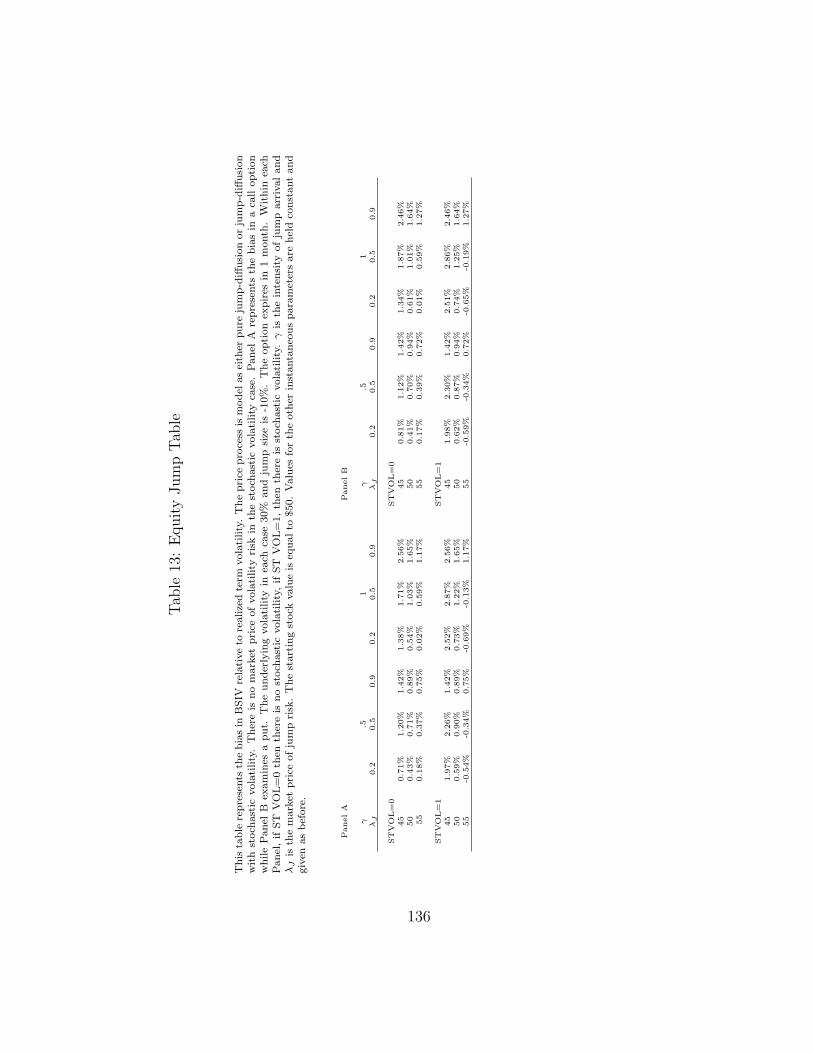
Tab
le13
:E
quity
Jum
pTab
le
This
table
repre
sents
the
bia
sin
BSIV
rela
tive
tore
alize
dte
rmvola
tility
.T
he
pri
cepro
cess
ism
odel
as
eith
erpure
jum
p-d
iffusi
on
or
jum
p-d
iffusi
on
wit
hst
och
ast
icvola
tility
.T
her
eis
no
mark
etpri
ceofvola
tility
risk
inth
est
och
ast
icvola
tility
case
.Panel
Are
pre
sents
the
bia
sin
aca
lloption
while
Panel
Bex
am
ines
aput.
The
under
lyin
gvola
tility
inea
chca
se30%
and
jum
psi
zeis
-10%
.T
he
option
expir
esin
1m
onth
.W
ithin
each
Panel
,if
ST
VO
L=
0th
enth
ere
isno
stoch
ast
icvola
tility
,if
ST
VO
L=
1,th
enth
ere
isst
och
ast
icvola
tility
.γ
isth
ein
tensi
tyofju
mp
arr
ivaland
λJ
isth
em
ark
etpri
ceofju
mp
risk
.T
he
start
ing
stock
valu
eis
equalto
$50.
Valu
esfo
rth
eoth
erin
stanta
neo
us
para
met
ers
are
hel
dco
nst
ant
and
giv
enas
bef
ore
.
PanelA
PanelB
γ.5
1γ
.51
λJ
0.2
0.5
0.9
0.2
0.5
0.9
λJ
0.2
0.5
0.9
0.2
0.5
0.9
ST
VO
L=
0ST
VO
L=
045
0.7
1%
1.2
0%
1.4
2%
1.3
8%
1.7
1%
2.5
6%
45
0.8
1%
1.1
2%
1.4
2%
1.3
4%
1.8
7%
2.4
6%
50
0.4
3%
0.7
1%
0.8
9%
0.5
4%
1.0
3%
1.6
5%
50
0.4
1%
0.7
0%
0.9
4%
0.6
1%
1.0
1%
1.6
4%
55
0.1
8%
0.3
7%
0.7
5%
0.0
2%
0.5
9%
1.1
7%
55
0.1
7%
0.3
9%
0.7
2%
0.0
1%
0.5
9%
1.2
7%
ST
VO
L=
1ST
VO
L=
145
1.9
7%
2.2
6%
1.4
2%
2.5
2%
2.8
7%
2.5
6%
45
1.9
8%
2.3
0%
1.4
2%
2.5
1%
2.8
6%
2.4
6%
50
0.5
9%
0.9
0%
0.8
9%
0.7
3%
1.2
2%
1.6
5%
50
0.6
2%
0.8
7%
0.9
4%
0.7
4%
1.2
5%
1.6
4%
55
-0.5
4%
-0.3
4%
0.7
5%
-0.6
9%
-0.1
3%
1.1
7%
55
-0.5
9%
-0.3
4%
0.7
2%
-0.6
5%
-0.1
9%
1.2
7%
136
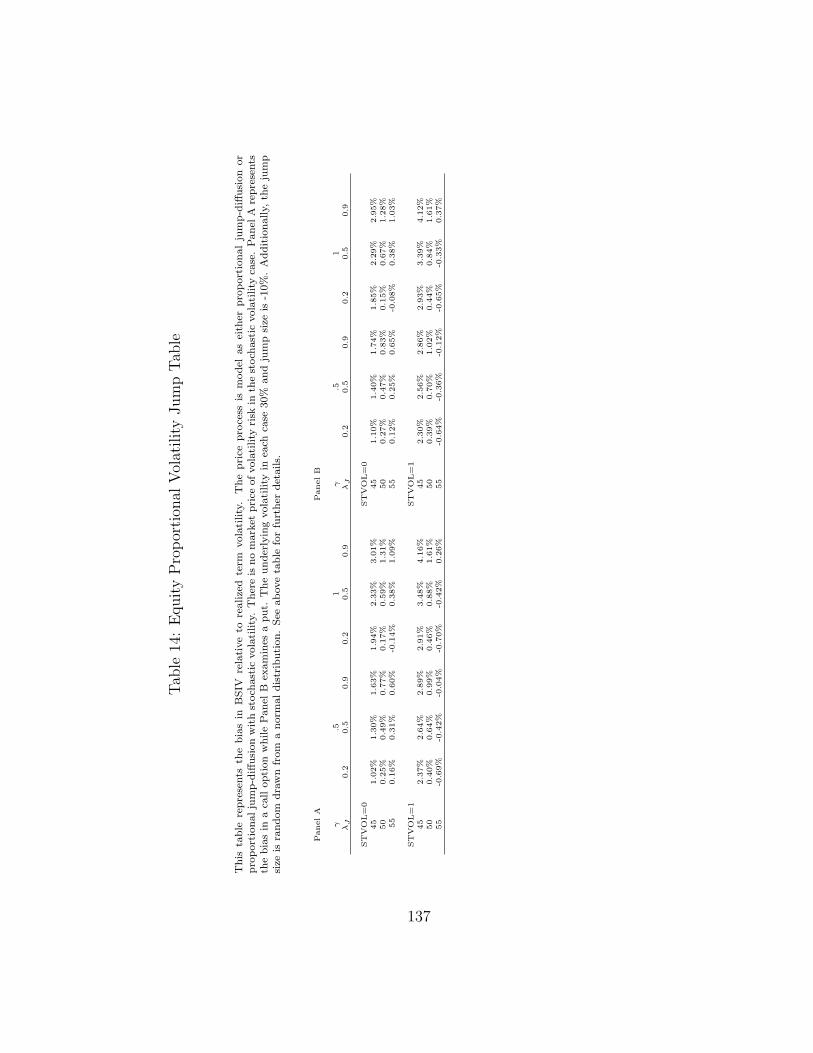
Tab
le14
:E
quity
Pro
por
tion
alV
olat
ility
Jum
pTab
le
This
table
repre
sents
the
bia
sin
BSIV
rela
tive
tore
alize
dte
rmvola
tility
.T
he
pri
cepro
cess
ism
odel
as
eith
erpro
port
ional
jum
p-d
iffusi
on
or
pro
port
ionalju
mp-d
iffusi
on
with
stoch
ast
icvola
tility
.T
her
eis
no
mark
etpri
ceofvola
tility
risk
inth
est
och
ast
icvola
tility
case
.Panel
Are
pre
sents
the
bia
sin
aca
llopti
on
while
Panel
Bex
am
ines
aput.
The
under
lyin
gvola
tility
inea
chca
se30%
and
jum
psi
zeis
-10%
.A
dditio
nally,
the
jum
psi
zeis
random
dra
wn
from
anorm
aldis
trib
uti
on.
See
above
table
for
furt
her
det
ails.
PanelA
PanelB
γ.5
1γ
.51
λJ
0.2
0.5
0.9
0.2
0.5
0.9
λJ
0.2
0.5
0.9
0.2
0.5
0.9
ST
VO
L=
0ST
VO
L=
045
1.0
2%
1.3
0%
1.6
3%
1.9
4%
2.3
3%
3.0
1%
45
1.1
0%
1.4
0%
1.7
4%
1.8
5%
2.2
9%
2.9
5%
50
0.2
5%
0.4
9%
0.7
7%
0.1
7%
0.5
9%
1.3
1%
50
0.2
7%
0.4
7%
0.8
3%
0.1
5%
0.6
7%
1.2
8%
55
0.1
6%
0.3
1%
0.6
0%
-0.1
4%
0.3
8%
1.0
9%
55
0.1
2%
0.2
5%
0.6
5%
-0.0
8%
0.3
8%
1.0
3%
ST
VO
L=
1ST
VO
L=
145
2.3
7%
2.6
4%
2.8
9%
2.9
1%
3.4
8%
4.1
6%
45
2.3
0%
2.5
6%
2.8
6%
2.9
3%
3.3
9%
4.1
2%
50
0.4
0%
0.6
4%
0.9
9%
0.4
6%
0.8
8%
1.6
1%
50
0.3
9%
0.7
0%
1.0
2%
0.4
4%
0.8
4%
1.6
1%
55
-0.6
9%
-0.4
2%
-0.0
4%
-0.7
0%
-0.4
2%
0.2
6%
55
-0.6
4%
-0.3
6%
-0.1
2%
-0.6
5%
-0.3
3%
0.3
7%
137

Table 15: Commodity Jump Table
This table represents the bias in BIV relative to realized term volatility for gas contracts. The futuresprocess is model as either pure jump-diffusion (Panel A) or jump-diffusion with stochastic volatility (PanelB). There is no market price of volatility risk in the stochastic volatility case. γ is the intensity of jumparrival and λJ is the market price of jump risk. The starting futures value is equal to $50. All otherparameters are fixed and initial values are the same as in prior simulations.
Panel A Panel BλJ .2 .5 .9 .2 .5 .9γ 0.5 1 0.5 1 0.5 1 0.5 1 0.5 1 0.5 140 0.18% 0.65% 0.89% 0.47% 1.35% 1.05% -0.86% -5.49% -1.16% -0.36% -0.32% -2.04%
0.62% 0.32% 0.87% 0.73% 1.18% 1.43% -0.95% -1.34% -0.81% -0.87% -0.39% -0.25%
42 0.46% 0.43% 1.11% 1.16% 1.10% 1.58% -0.38% -1.17% -0.81% -0.04% 0.26% 0.13%0.71% 0.43% 0.93% 0.89% 1.28% 1.56% -0.77% -1.00% -0.50% -0.56% -0.19% 0.12%
44 0.78% 0.57% 0.94% 0.89% 1.39% 1.74% -0.48% -0.57% -0.08% -0.30% 0.09% 0.57%0.79% 0.61% 1.04% 1.08% 1.34% 1.70% -0.34% -0.52% -0.11% -0.03% 0.20% 0.59%
45 0.78% 0.63% 1.15% 1.28% 1.29% 1.71% -0.08% -0.24% 0.03% 0.33% 0.45% 0.81%0.84% 0.71% 1.04% 1.11% 1.38% 1.78% -0.17% -0.26% 0.12% 0.16% 0.39% 0.86%
46 0.91% 0.79% 1.07% 1.18% 1.47% 1.90% 0.05% 0.02% 0.38% 0.43% 0.62% 1.15%0.87% 0.74% 1.11% 1.21% 1.43% 1.87% 0.07% 0.00% 0.31% 0.44% 0.63% 1.09%
47 0.91% 0.86% 1.06% 1.22% 1.46% 1.94% 0.22% 0.25% 0.56% 0.64% 0.81% 1.36%0.91% 0.83% 1.08% 1.26% 1.47% 1.92% 0.24% 0.24% 0.57% 0.70% 0.81% 1.36%
48 0.90% 0.86% 1.22% 1.43% 1.47% 1.97% 0.60% 0.50% 0.71% 1.08% 1.13% 1.58%0.95% 0.93% 1.18% 1.38% 1.50% 2.02% 0.57% 0.56% 0.75% 1.05% 1.12% 1.64%
49 1.02% 1.06% 1.25% 1.52% 1.59% 2.15% 0.78% 0.83% 1.05% 1.31% 1.33% 1.97%0.98% 0.98% 1.28% 1.52% 1.55% 2.10% 0.80% 0.79% 1.00% 1.29% 1.36% 1.89%
50 1.08% 1.13% 1.31% 1.62% 1.63% 2.25% 1.01% 1.16% 1.32% 1.57% 1.59% 2.27%1.08% 1.16% 1.30% 1.62% 1.64% 2.25% 1.01% 1.14% 1.31% 1.59% 1.57% 2.27%
51 1.10% 1.23% 1.36% 1.69% 1.67% 2.30% 1.30% 1.38% 1.49% 1.87% 1.84% 2.46%1.14% 1.28% 1.34% 1.69% 1.70% 2.38% 1.28% 1.45% 1.54% 1.87% 1.82% 2.56%
52 1.20% 1.33% 1.37% 1.79% 1.75% 2.50% 1.50% 1.70% 1.76% 2.13% 2.03% 2.80%1.15% 1.26% 1.42% 1.82% 1.71% 2.41% 1.55% 1.62% 1.72% 2.16% 2.08% 2.72%
53 1.23% 1.43% 1.50% 1.94% 1.76% 2.53% 1.76% 1.94% 1.96% 2.42% 2.33% 3.02%1.25% 1.45% 1.47% 1.92% 1.78% 2.54% 1.72% 1.95% 1.97% 2.38% 2.29% 3.03%
54 1.20% 1.56% 1.53% 2.05% 1.81% 2.63% 2.00% 2.12% 2.14% 2.72% 2.53% 3.26%1.24% 1.54% 1.54% 2.05% 1.82% 2.66% 1.99% 2.20% 2.15% 2.70% 2.52% 3.28%
55 1.42% 1.70% 1.55% 2.11% 1.94% 2.81% 2.11% 2.47% 2.49% 2.83% 2.69% 3.57%1.34% 1.75% 1.60% 2.18% 1.90% 2.77% 2.16% 2.38% 2.46% 2.91% 2.75% 3.56%
56 1.43% 1.84% 1.70% 2.30% 2.00% 2.95% 2.43% 2.71% 2.62% 3.20% 2.99% 3.81%1.52% 1.82% 1.63% 2.21% 2.05% 2.95% 2.35% 2.74% 2.67% 3.09% 2.89% 3.80%
58 1.64% 2.10% 1.83% 2.58% 2.22% 3.23% 2.80% 3.15% 3.12% 3.66% 3.35% 4.29%1.63% 2.11% 1.96% 2.81% 2.17% 3.22% 2.95% 3.18% 3.10% 3.90% 3.45% 4.30%
60 1.82% 2.42% 2.06% 2.83% 2.40% 3.54% 3.22% 3.62% 3.45% 4.08% 3.78% 4.70%1.68% 2.18% 2.17% 2.92% 2.20% 3.38% 3.32% 3.51% 3.24% 4.09% 3.89% 4.55%
138

Table 16: Commodity Proportional Volatility Jump Table
This table represents the bias in BIV relative to realized term volatility for gas contracts. The futures processis model as either proportional jump-diffusion (Panel A) or proportional jump-diffusion with stochasticvolatility (Panel B). There is no market price of volatility risk in the stochastic volatility case. γ is theintensity of jump arrival and λJ is the market price of jump risk. The starting futures value is equal to $50.All other parameters are fixed and initial values are the same as in prior simulations.
Panel A Panel BλJ .2 .5 .9 .2 .5 .9γ 0.5 1 0.5 1 0.5 1 0.5 1 0.5 1 0.5 1
40 0.92% 1.74% 1.15% 2.51% 1.45% 3.03% 1.57% 0.96% -0.02% 1.44% 2.15% 2.55%1.96% 2.35% 2.18% 2.93% 2.49% 3.47% 0.69% 1.36% 0.96% 1.83% 1.20% 2.50%
42 1.05% 1.24% 1.26% 1.97% 1.57% 2.25% 0.16% 0.13% 0.07% 0.55% 0.75% 1.44%1.20% 1.29% 1.42% 1.74% 1.73% 2.31% -0.10% 0.03% 0.06% 0.44% 0.42% 1.12%
44 1.01% 0.94% 1.24% 1.33% 1.54% 1.96% -0.32% -0.23% 0.07% 0.19% 0.25% 0.76%0.91% 0.87% 1.14% 1.34% 1.43% 1.92% -0.19% -0.23% 0.03% 0.19% 0.36% 0.81%
45 0.89% 0.80% 1.10% 1.37% 1.40% 1.84% 0.05% -0.14% 0.14% 0.30% 0.57% 0.97%0.92% 0.78% 1.13% 1.25% 1.43% 1.81% -0.08% -0.16% 0.18% 0.28% 0.47% 0.87%
46 0.79% 0.63% 1.02% 1.17% 1.32% 1.69% 0.15% -0.19% 0.20% 0.26% 0.67% 0.97%0.82% 0.69% 1.05% 1.24% 1.35% 1.73% 0.08% -0.10% 0.25% 0.36% 0.59% 1.00%
47 0.92% 0.82% 1.15% 1.16% 1.45% 1.84% 0.19% 0.25% 0.59% 0.66% 0.70% 1.16%0.91% 0.83% 1.14% 1.18% 1.44% 1.84% 0.23% 0.23% 0.53% 0.64% 0.75% 1.17%
48 0.90% 0.83% 1.12% 1.26% 1.42% 1.85% 0.45% 0.44% 0.71% 0.88% 1.01% 1.42%0.92% 0.78% 1.14% 1.22% 1.44% 1.81% 0.42% 0.37% 0.71% 0.82% 0.97% 1.38%
49 0.92% 0.84% 1.14% 1.27% 1.45% 1.91% 0.64% 0.64% 0.92% 1.07% 1.18% 1.65%0.90% 0.81% 1.12% 1.27% 1.43% 1.88% 0.67% 0.60% 0.89% 1.03% 1.19% 1.63%
50 1.02% 0.99% 1.25% 1.29% 1.55% 2.00% 0.86% 0.99% 1.24% 1.40% 1.36% 1.83%1.01% 1.02% 1.24% 1.33% 1.54% 2.05% 0.89% 0.99% 1.20% 1.40% 1.41% 1.91%
51 1.02% 1.04% 1.24% 1.49% 1.54% 2.12% 1.20% 1.19% 1.40% 1.65% 1.72% 2.26%1.07% 1.05% 1.29% 1.47% 1.59% 2.12% 1.21% 1.20% 1.43% 1.66% 1.71% 2.26%
52 1.18% 1.26% 1.42% 1.65% 1.73% 2.33% 1.43% 1.61% 1.76% 2.05% 1.96% 2.59%1.14% 1.21% 1.37% 1.63% 1.68% 2.25% 1.45% 1.57% 1.71% 2.01% 1.98% 2.58%
53 1.24% 1.43% 1.45% 1.76% 1.75% 2.43% 1.70% 1.98% 2.01% 2.38% 2.21% 2.88%1.23% 1.47% 1.44% 1.78% 1.74% 2.49% 1.69% 1.99% 1.96% 2.40% 2.22% 2.93%
54 1.26% 1.53% 1.49% 2.08% 1.79% 2.64% 2.09% 2.23% 2.19% 2.71% 2.63% 3.41%1.34% 1.56% 1.57% 2.09% 1.87% 2.65% 2.03% 2.24% 2.24% 2.72% 2.58% 3.38%
55 1.52% 1.96% 1.76% 2.41% 2.06% 2.98% 2.31% 2.76% 2.61% 3.19% 2.85% 3.83%1.44% 1.89% 1.68% 2.35% 1.98% 2.95% 2.34% 2.69% 2.54% 3.13% 2.85% 3.76%
56 1.64% 2.28% 1.86% 2.77% 2.17% 3.32% 2.75% 3.21% 2.85% 3.63% 3.26% 4.31%1.68% 2.28% 1.90% 2.70% 2.21% 3.34% 2.67% 3.18% 2.85% 3.60% 3.20% 4.24%
58 2.34% 3.34% 2.56% 3.73% 2.86% 4.36% 3.34% 4.37% 3.73% 4.79% 3.92% 5.35%2.22% 3.28% 2.45% 3.69% 2.74% 4.35% 3.47% 4.35% 3.69% 4.78% 3.99% 5.34%
60 3.22% 4.68% 3.44% 5.13% 3.74% 5.79% 4.51% 5.66% 4.67% 6.11% 5.04% 6.74%3.29% 4.83% 3.52% 5.30% 3.82% 5.79% 4.28% 5.89% 4.79% 6.34% 4.78% 6.77%
139
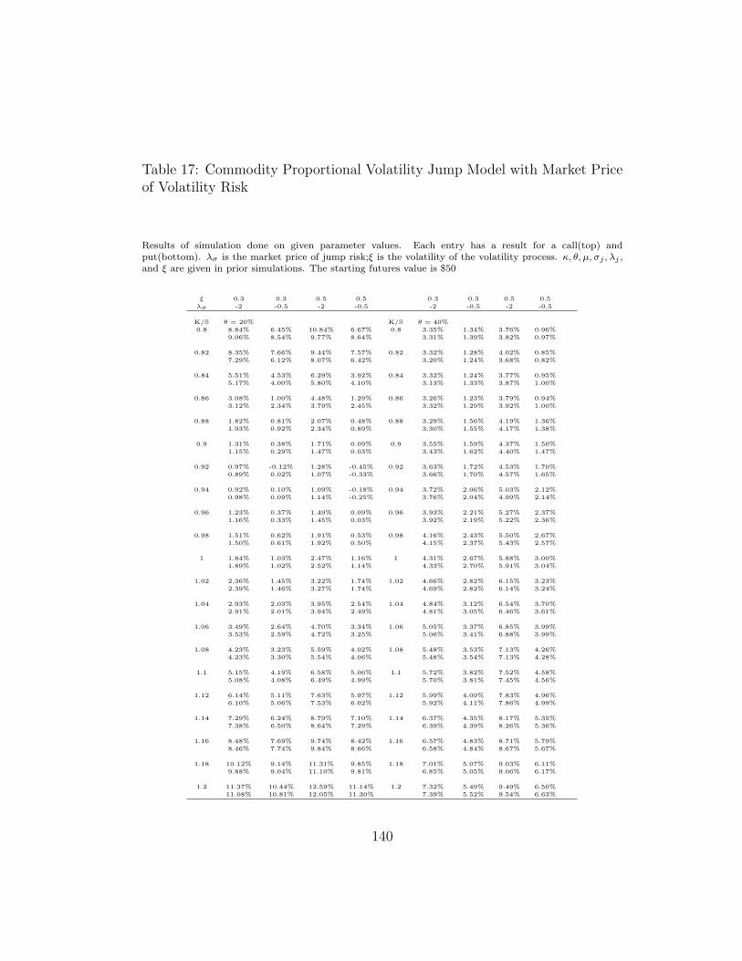
Table 17: Commodity Proportional Volatility Jump Model with Market Priceof Volatility Risk
Results of simulation done on given parameter values. Each entry has a result for a call(top) andput(bottom). λσ is the market price of jump risk;ξ is the volatility of the volatility process. κ, θ, µ, σj , λj ,and ξ are given in prior simulations. The starting futures value is $50
ξ 0.3 0.3 0.5 0.5 0.3 0.3 0.5 0.5λσ -2 -0.5 -2 -0.5 -2 -0.5 -2 -0.5
K/S θ = 20% K/S θ = 40%0.8 8.84% 6.45% 10.84% 6.67% 0.8 3.35% 1.34% 3.76% 0.96%
9.06% 8.54% 9.77% 8.64% 3.31% 1.39% 3.82% 0.97%
0.82 8.35% 7.66% 9.44% 7.57% 0.82 3.32% 1.28% 4.02% 0.85%7.29% 6.12% 8.07% 6.42% 3.20% 1.24% 3.68% 0.82%
0.84 5.51% 4.53% 6.29% 3.92% 0.84 3.32% 1.24% 3.77% 0.95%5.17% 4.00% 5.80% 4.10% 3.13% 1.33% 3.87% 1.00%
0.86 3.08% 1.00% 4.48% 1.29% 0.86 3.26% 1.23% 3.79% 0.94%3.12% 2.34% 3.79% 2.45% 3.32% 1.29% 3.92% 1.00%
0.88 1.82% 0.81% 2.07% 0.48% 0.88 3.29% 1.56% 4.19% 1.36%1.93% 0.92% 2.34% 0.89% 3.30% 1.55% 4.17% 1.38%
0.9 1.31% 0.38% 1.71% 0.09% 0.9 3.55% 1.59% 4.37% 1.50%1.15% 0.29% 1.47% 0.03% 3.43% 1.62% 4.40% 1.47%
0.92 0.97% -0.12% 1.28% -0.45% 0.92 3.63% 1.72% 4.53% 1.70%0.89% 0.02% 1.07% -0.33% 3.66% 1.70% 4.57% 1.65%
0.94 0.92% 0.10% 1.09% -0.18% 0.94 3.72% 2.06% 5.03% 2.12%0.98% 0.09% 1.14% -0.25% 3.76% 2.04% 4.99% 2.14%
0.96 1.23% 0.37% 1.49% 0.09% 0.96 3.93% 2.21% 5.27% 2.37%1.16% 0.33% 1.45% 0.03% 3.92% 2.19% 5.22% 2.36%
0.98 1.51% 0.62% 1.91% 0.53% 0.98 4.16% 2.43% 5.50% 2.67%1.50% 0.61% 1.92% 0.50% 4.15% 2.37% 5.43% 2.57%
1 1.84% 1.03% 2.47% 1.16% 1 4.31% 2.67% 5.88% 3.00%1.89% 1.02% 2.52% 1.14% 4.33% 2.70% 5.91% 3.04%
1.02 2.36% 1.45% 3.22% 1.74% 1.02 4.66% 2.82% 6.15% 3.23%2.39% 1.46% 3.27% 1.74% 4.69% 2.82% 6.14% 3.24%
1.04 2.93% 2.03% 3.95% 2.54% 1.04 4.84% 3.12% 6.54% 3.70%2.91% 2.01% 3.94% 2.49% 4.81% 3.05% 6.46% 3.61%
1.06 3.49% 2.64% 4.70% 3.34% 1.06 5.05% 3.37% 6.85% 3.99%3.53% 2.59% 4.72% 3.25% 5.06% 3.41% 6.88% 3.99%
1.08 4.23% 3.23% 5.59% 4.02% 1.08 5.48% 3.53% 7.13% 4.26%4.23% 3.30% 5.54% 4.06% 5.48% 3.54% 7.13% 4.28%
1.1 5.15% 4.19% 6.58% 5.06% 1.1 5.72% 3.82% 7.52% 4.58%5.08% 4.08% 6.49% 4.99% 5.70% 3.81% 7.45% 4.56%
1.12 6.14% 5.11% 7.63% 5.97% 1.12 5.99% 4.09% 7.83% 4.96%6.10% 5.06% 7.53% 6.02% 5.92% 4.11% 7.86% 4.99%
1.14 7.29% 6.24% 8.79% 7.10% 1.14 6.37% 4.35% 8.17% 5.35%7.38% 6.50% 8.64% 7.29% 6.39% 4.39% 8.26% 5.36%
1.16 8.48% 7.69% 9.74% 8.42% 1.16 6.57% 4.83% 8.71% 5.79%8.46% 7.74% 9.84% 8.66% 6.58% 4.84% 8.67% 5.67%
1.18 10.12% 9.14% 11.31% 9.85% 1.18 7.01% 5.07% 9.03% 6.11%9.88% 9.04% 11.10% 9.81% 6.85% 5.05% 9.06% 6.17%
1.2 11.37% 10.44% 12.59% 11.14% 1.2 7.32% 5.49% 9.49% 6.50%11.08% 10.81% 12.05% 11.30% 7.39% 5.52% 9.54% 6.63%
140

Table 18: Mean-Reversion regression of instantaneous volatility and BSIVfrom 30 day options
InstVol is the mean reversion regression run on instantaneous volatility (input to the simulation). BSIV-call/BSIVput is the mean reversion regression done on implied volatility from the call/put. The dependentvariable is change in volatility from t to t− 1. For each case λσ = 0 except for the last where λσ = −2. Theinferred values are backed out from the coefficent estimates.
4σ2 4σ2 4σ2 4σ2
InstVol -0.022 -0.036(5.53)** (6.47)**
BSIVcall -0.022(5.53)**
BSIVput -0.022(5.52)**
Constant 0.000678 0.00072 0.000718 0.000705(4.91)** (5.16)** (5.16)** (5.73)**
Observations 2708 2708 2708 2214R-squared 0.01 0.01 0.01 0.02
Absolute value of t statistics in parentheses* significant at 5%; ** significant at 1%
Inferred Values
λσ = 0 λσ = −2κ 5.61 5.61θ 17.08% 17.75%λσ 0 -1.78
141
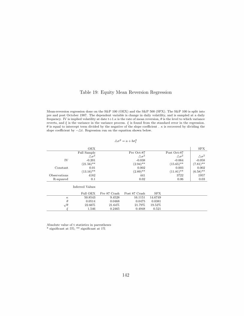
Table 19: Equity Mean Reversion Regression
Mean-reversion regression done on the S&P 100 (OEX) and the S&P 500 (SPX). The S&P 100 is split intopre and post October 1987. The dependent variable is change in daily volatility, and is sampled at a dailyfrequency. IV is implied volatility at date t+1.κ is the rate of mean reversion, θ is the level to which variancereverts, and ξ is the variance in the variance process. ξ is found from the standard error in the regression.θ is equal to intercept term divided by the negative of the slope coefficient . κ is recovered by dividing theslope coefficient by −4t. Regression run on the equation shown below.
4σ2 = a + bσ2t
OEX SPXFull Sample Pre Oct-87 Post Oct-87
4σ2 4σ2 4σ2 4σ2
IV -0.201 -0.038 -0.064 -0.058(21.56)** (2.94)** (15.65)** (7.81)**
Constant 0.01 0.002 0.003 0.002(13.16)** (2.89)** (11.81)** (6.58)**
Observations 4182 441 3722 1957R-squared 0.1 0.02 0.06 0.03
Inferred Values
Full OEX Pre 87 Crash Post 87 Crash SPXκ 50.8543 9.4528 16.1151 14.6749θ 0.0514 0.0468 0.0475 0.0381√θ 22.66% 21.64% 21.79% 19.52%ξ 1.546 0.2465 0.4948 0.521
Absolute value of t statistics in parentheses* significant at 5%; ** significant at 1%
142
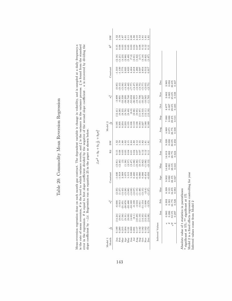
Tab
le20
:C
omm
odity
Mea
nR
ever
sion
Reg
ress
ion
Mea
n-r
ever
sion
regre
ssio
ndone
on
each
month
gas
contr
act
.T
he
dep
enden
tvari
able
isch
ange
invola
tility
,and
issa
mple
dat
adaily
freq
uen
cy.κ
isth
era
teofm
ean
rever
sion,
θis
the
level
tow
hic
hvari
ance
rever
ts,and
ξis
the
vari
ance
inth
evari
ance
pro
cess
.ξ
isfo
und
from
the
standard
erro
rin
the
regre
ssio
n.
θis
equalto
firs
tsl
ope
coeffi
cien
tdiv
ided
by
the
neg
ati
ve
of
the
seco
nd
slope
coeffi
cien
t.
κis
reco
ver
edby
div
idin
gth
esl
ope
coeffi
cien
tby−4
t.R
egre
ssio
nru
non
equation
25
inth
epaper
as
show
nbel
ow
.
4σ
2=
b 0+
b 11 t2
+b 2
σ2 t
Model1
Model2
Month
1 t2
σ2 t
Const
ant
R2
DW
1 t2
σ2 t
Const
ant
R2
DW
Jan
0.1
89
(14.2
4)
-6.6
66
(2.3
5)
-1.6
46
-(3.8
1)
0.1
51.3
20.1
95
(12.4
1)
-3.8
99
(0.8
5)
-1.3
10
-(2.1
6)
0.1
51.3
2
Feb
0.2
80
(9.8
1)
-5.9
13
(1.2
7)
-1.9
18
-(2.4
6)
0.0
81.7
90.3
05
(9.3
8)
-0.8
01
-(0.1
3)
-1.1
30
-(1.2
1)
0.0
81.7
8
Mar
0.2
15
(7.5
6)
-21.3
51
-(4.4
3)
2.3
69
(3)
0.0
31.8
80.2
54
(8.2
3)
-33.3
30
-(5.5
6)
3.7
75
(4.2
3)
0.0
31.8
7
Apr
0.2
04
(9.3
1)
-20.8
76
-(3.2
8)
1.0
75
(1.3
8)
0.0
51.6
20.2
33
(9.7
6)
-39.2
95
-(4.3
4)
2.9
25
(2.8
8)
0.0
51.6
1
May
0.1
21
(8.0
9)
-22.4
86
-(3.8
6)
1.5
15
(2.5
7)
0.0
42.1
50.1
55
(9.4
9)
-58.7
40
-(6.4
2)
4.6
23
(5.4
9)
0.0
52.1
1
Jun
0.0
69
(4.8
3)
-18.1
89
-(4.0
8)
1.5
06
(3.4
7)
0.0
12.2
40.1
06
(6.9
)-5
5.6
32
-(7.7
7)
4.4
64
(7.2
)0.0
32.2
0
Jul
0.0
91
(8.1
)-8
.199
-(2.0
7)
0.4
80
(1.0
8)
0.0
41.8
90.1
19
(8.9
8)
-36.9
85
-(4.4
7)
3.2
18
(3.9
1)
0.0
41.8
6
Aug
0.1
17
(10.2
9)
-4.5
34
-(1.1
5)
-0.1
61
-(0.3
6)
0.0
72.1
20.1
36
(9.9
5)
-19.7
17
-(2.5
6)
1.2
66
(1.6
2)
0.0
72.1
0
Sep
0.1
42
(11.1
9)
-5.8
11
-(1.4
8)
0.0
80
(0.1
7)
0.0
71.5
50.1
84
(11.9
7)
-31.7
06
-(4.7
5)
2.5
97
(3.7
)0.0
81.5
3
Oct
0.1
82
(14.3
5)
-11.1
54
-(3.1
5)
0.3
66
(0.8
2)
0.1
21.8
20.2
27
(14.5
3)
-35.2
27
-(5.7
7)
2.8
54
(4.1
8)
0.1
21.8
1
Nov
0.1
62
(13.2
5)
-1.8
98
-(0.6
)-0
.454
-(1.0
6)
0.1
21.8
10.1
80
(12.1
1)
-10.5
65
-(2.0
3)
0.5
12
(0.8
2)
0.1
21.8
1
Dec
0.1
70
(14.0
8)
-3.5
76
-(1.2
7)
-0.0
50
-(0.1
3)
0.1
11.8
10.1
89
(13.1
8)
-11.7
65
-(2.7
5)
0.9
17
(1.6
7)
0.1
11.8
1
Infe
rred
Valu
es
Jan
Feb
Mar
Apr
May
Jun
Jul
Aug
Sep
Oct
Nov
Dec
κ0.9
83
0.2
02
8.3
99
9.9
02
14.8
02
14.0
19
9.3
20
4.9
69
7.9
90
8.8
77
2.6
62
2.9
65
θ0.2
86
0.3
81
0.1
21
0.0
80
0.0
81
0.0
82
0.0
90
0.0
71
0.0
88
0.0
87
0.0
65
0.0
94
√θ
53.5
%61.7
%34.8
%28.3
%28.5
%28.7
%30.0
%26.7
%29.6
%29.6
%25.6
%30.6
%
ξ0.2
97
0.5
26
0.9
83
0.9
27
0.6
45
0.6
24
0.4
56
0.5
08
0.5
15
0.4
85
0.5
38
0.4
47
Abso
lute
valu
eoft
statist
ics
inpare
nth
eses
*si
gnifi
cant
at
5%
;**
signifi
cant
at
1%
Model
2is
afixed
effec
tsre
gre
ssio
nco
ntr
ollin
gfo
ryea
rIn
ferr
edvalu
esco
me
from
Model
2
143
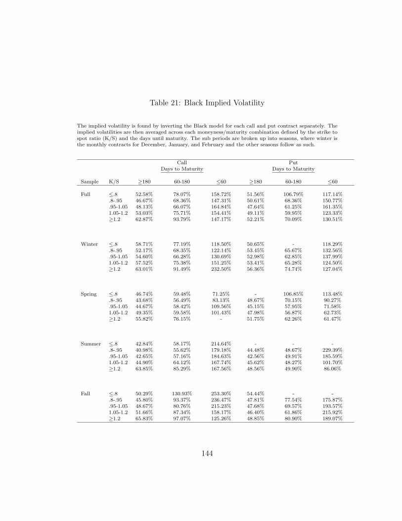
Table 21: Black Implied Volatility
The implied volatility is found by inverting the Black model for each call and put contract separately. Theimplied volatilities are then averaged across each moneyness/maturity combination defined by the strike tospot ratio (K/S) and the days until maturity. The sub periods are broken up into seasons, where winter isthe monthly contracts for December, January, and February and the other seasons follow as such.
Call PutDays to Maturity Days to Maturity
Sample K/S ≥180 60-180 ≤60 ≥180 60-180 ≤60
Full ≤.8 52.58% 78.07% 158.72% 51.56% 106.79% 117.14%.8-.95 46.67% 68.36% 147.31% 50.61% 68.36% 150.77%.95-1.05 48.13% 66.07% 164.84% 47.64% 61.25% 161.35%1.05-1.2 53.03% 75.71% 154.41% 49.11% 59.95% 123.33%≥1.2 62.87% 93.79% 147.17% 52.21% 70.09% 130.51%
Winter ≤.8 58.71% 77.19% 118.50% 50.65% - 118.29%.8-.95 52.17% 68.35% 122.14% 53.45% 65.67% 132.56%.95-1.05 54.60% 66.28% 130.69% 52.98% 62.85% 137.99%1.05-1.2 57.52% 75.38% 151.25% 53.41% 65.28% 124.50%≥1.2 63.01% 91.49% 232.50% 56.36% 74.74% 127.04%
Spring ≤.8 46.74% 59.48% 71.25% - 106.85% 113.48%.8-.95 43.68% 56.49% 83.13% 48.67% 70.15% 90.27%.95-1.05 44.67% 58.42% 109.56% 45.15% 57.95% 71.58%1.05-1.2 49.35% 59.58% 101.43% 47.98% 56.87% 62.73%≥1.2 55.82% 76.15% - 51.75% 62.26% 61.47%
Summer ≤.8 42.84% 58.17% 214.64% - - -.8-.95 40.98% 55.62% 179.18% 44.48% 48.67% 229.39%.95-1.05 42.65% 57.16% 184.63% 42.56% 49.91% 185.59%1.05-1.2 44.90% 64.12% 167.74% 45.62% 48.27% 101.70%≥1.2 63.85% 85.29% 167.56% 48.56% 49.90% 86.06%
Fall ≤.8 50.29% 130.93% 253.30% 54.44% - -.8-.95 45.80% 93.37% 236.47% 47.81% 77.54% 175.87%.95-1.05 48.67% 80.76% 215.23% 47.68% 69.57% 193.57%1.05-1.2 51.66% 87.34% 158.17% 46.40% 61.86% 215.92%≥1.2 65.83% 97.07% 125.26% 48.85% 80.90% 189.07%
144
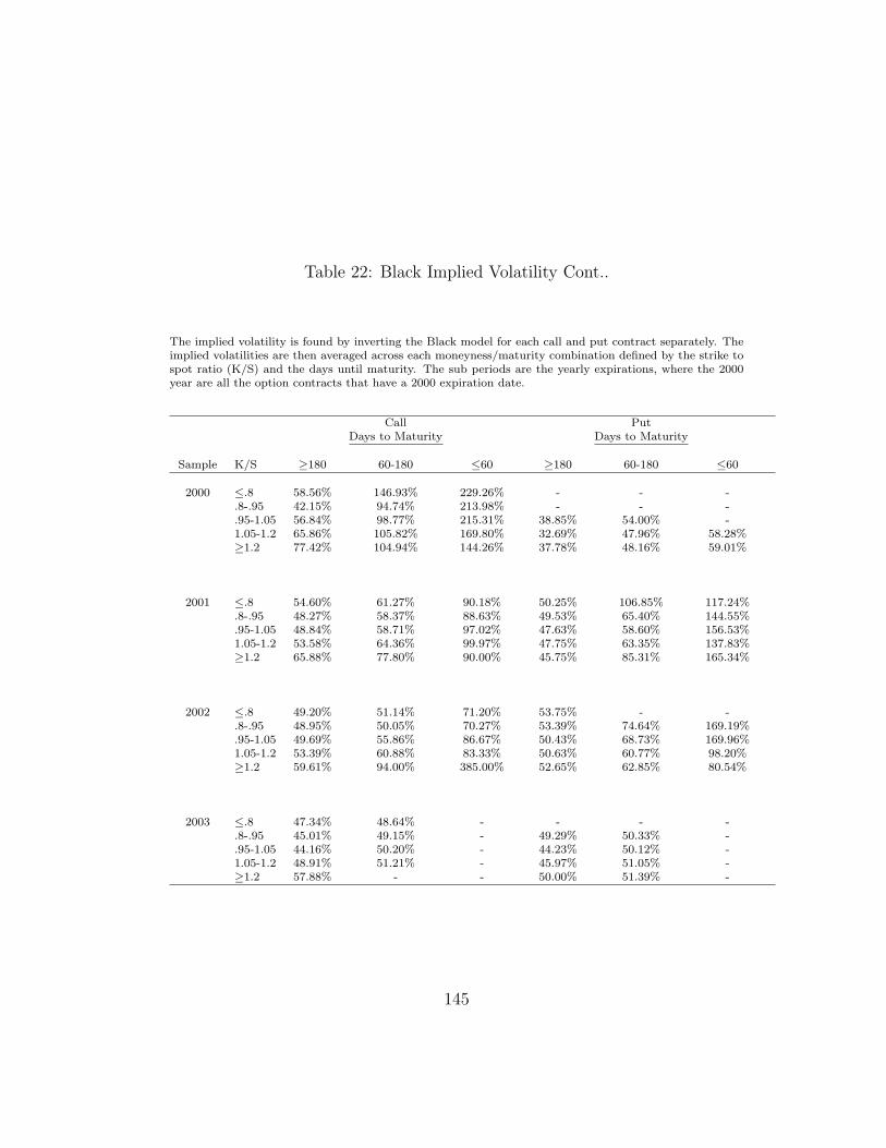
Table 22: Black Implied Volatility Cont..
The implied volatility is found by inverting the Black model for each call and put contract separately. Theimplied volatilities are then averaged across each moneyness/maturity combination defined by the strike tospot ratio (K/S) and the days until maturity. The sub periods are the yearly expirations, where the 2000year are all the option contracts that have a 2000 expiration date.
Call PutDays to Maturity Days to Maturity
Sample K/S ≥180 60-180 ≤60 ≥180 60-180 ≤60
2000 ≤.8 58.56% 146.93% 229.26% - - -.8-.95 42.15% 94.74% 213.98% - - -.95-1.05 56.84% 98.77% 215.31% 38.85% 54.00% -1.05-1.2 65.86% 105.82% 169.80% 32.69% 47.96% 58.28%≥1.2 77.42% 104.94% 144.26% 37.78% 48.16% 59.01%
2001 ≤.8 54.60% 61.27% 90.18% 50.25% 106.85% 117.24%.8-.95 48.27% 58.37% 88.63% 49.53% 65.40% 144.55%.95-1.05 48.84% 58.71% 97.02% 47.63% 58.60% 156.53%1.05-1.2 53.58% 64.36% 99.97% 47.75% 63.35% 137.83%≥1.2 65.88% 77.80% 90.00% 45.75% 85.31% 165.34%
2002 ≤.8 49.20% 51.14% 71.20% 53.75% - -.8-.95 48.95% 50.05% 70.27% 53.39% 74.64% 169.19%.95-1.05 49.69% 55.86% 86.67% 50.43% 68.73% 169.96%1.05-1.2 53.39% 60.88% 83.33% 50.63% 60.77% 98.20%≥1.2 59.61% 94.00% 385.00% 52.65% 62.85% 80.54%
2003 ≤.8 47.34% 48.64% - - - -.8-.95 45.01% 49.15% - 49.29% 50.33% -.95-1.05 44.16% 50.20% - 44.23% 50.12% -1.05-1.2 48.91% 51.21% - 45.97% 51.05% -≥1.2 57.88% - - 50.00% 51.39% -
145
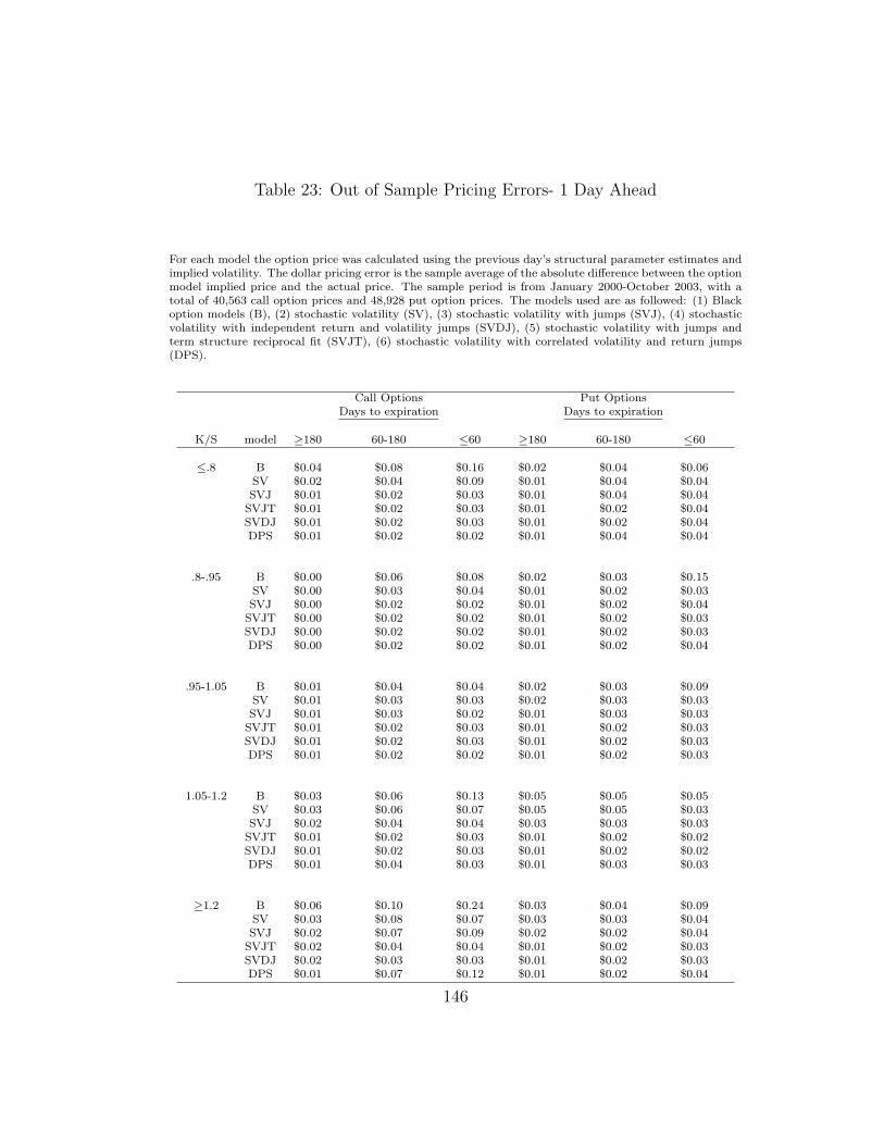
Table 23: Out of Sample Pricing Errors- 1 Day Ahead
For each model the option price was calculated using the previous day’s structural parameter estimates andimplied volatility. The dollar pricing error is the sample average of the absolute difference between the optionmodel implied price and the actual price. The sample period is from January 2000-October 2003, with atotal of 40,563 call option prices and 48,928 put option prices. The models used are as followed: (1) Blackoption models (B), (2) stochastic volatility (SV), (3) stochastic volatility with jumps (SVJ), (4) stochasticvolatility with independent return and volatility jumps (SVDJ), (5) stochastic volatility with jumps andterm structure reciprocal fit (SVJT), (6) stochastic volatility with correlated volatility and return jumps(DPS).
Call Options Put OptionsDays to expiration Days to expiration
K/S model ≥180 60-180 ≤60 ≥180 60-180 ≤60
≤.8 B $0.04 $0.08 $0.16 $0.02 $0.04 $0.06SV $0.02 $0.04 $0.09 $0.01 $0.04 $0.04SVJ $0.01 $0.02 $0.03 $0.01 $0.04 $0.04
SVJT $0.01 $0.02 $0.03 $0.01 $0.02 $0.04SVDJ $0.01 $0.02 $0.03 $0.01 $0.02 $0.04DPS $0.01 $0.02 $0.02 $0.01 $0.04 $0.04
.8-.95 B $0.00 $0.06 $0.08 $0.02 $0.03 $0.15SV $0.00 $0.03 $0.04 $0.01 $0.02 $0.03SVJ $0.00 $0.02 $0.02 $0.01 $0.02 $0.04
SVJT $0.00 $0.02 $0.02 $0.01 $0.02 $0.03SVDJ $0.00 $0.02 $0.02 $0.01 $0.02 $0.03DPS $0.00 $0.02 $0.02 $0.01 $0.02 $0.04
.95-1.05 B $0.01 $0.04 $0.04 $0.02 $0.03 $0.09SV $0.01 $0.03 $0.03 $0.02 $0.03 $0.03SVJ $0.01 $0.03 $0.02 $0.01 $0.03 $0.03
SVJT $0.01 $0.02 $0.03 $0.01 $0.02 $0.03SVDJ $0.01 $0.02 $0.03 $0.01 $0.02 $0.03DPS $0.01 $0.02 $0.02 $0.01 $0.02 $0.03
1.05-1.2 B $0.03 $0.06 $0.13 $0.05 $0.05 $0.05SV $0.03 $0.06 $0.07 $0.05 $0.05 $0.03SVJ $0.02 $0.04 $0.04 $0.03 $0.03 $0.03
SVJT $0.01 $0.02 $0.03 $0.01 $0.02 $0.02SVDJ $0.01 $0.02 $0.03 $0.01 $0.02 $0.02DPS $0.01 $0.04 $0.03 $0.01 $0.03 $0.03
≥1.2 B $0.06 $0.10 $0.24 $0.03 $0.04 $0.09SV $0.03 $0.08 $0.07 $0.03 $0.03 $0.04SVJ $0.02 $0.07 $0.09 $0.02 $0.02 $0.04
SVJT $0.02 $0.04 $0.04 $0.01 $0.02 $0.03SVDJ $0.02 $0.03 $0.03 $0.01 $0.02 $0.03DPS $0.01 $0.07 $0.12 $0.01 $0.02 $0.04
146
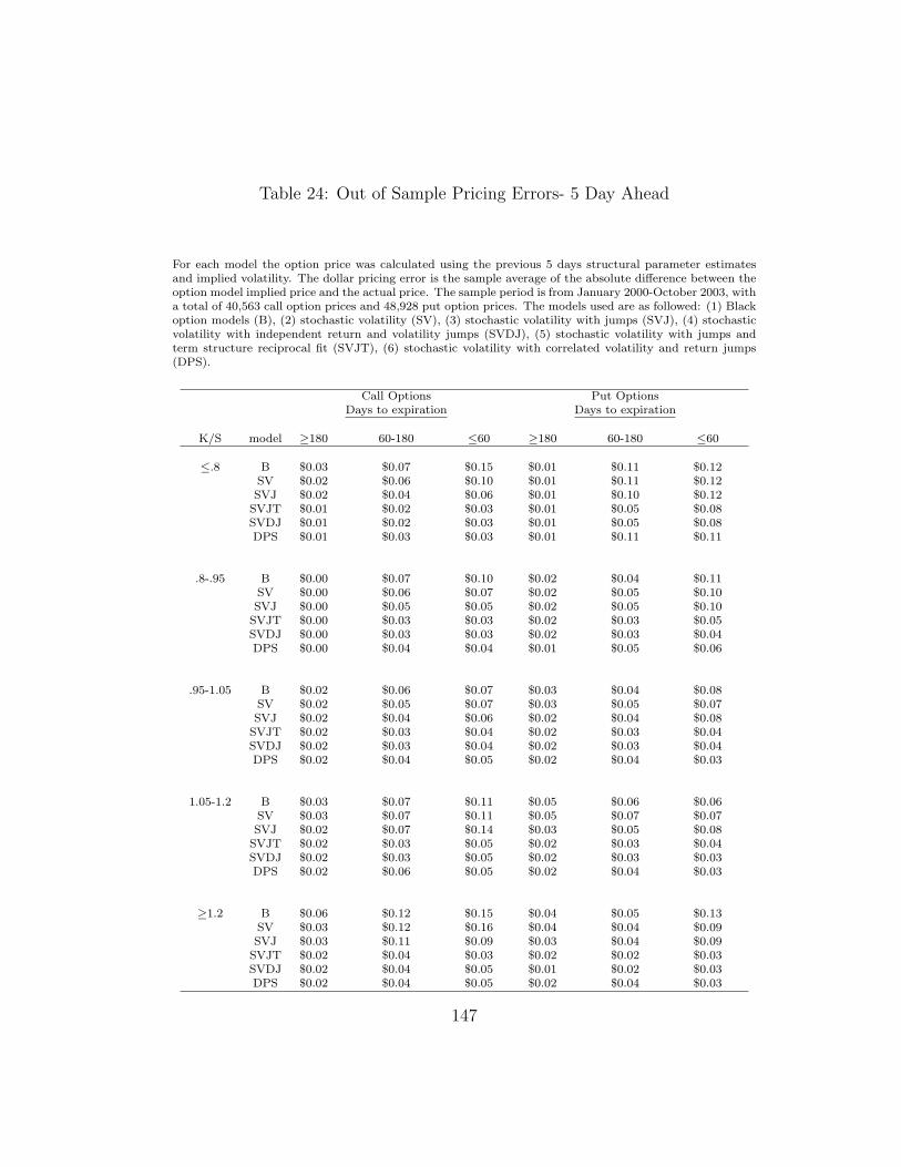
Table 24: Out of Sample Pricing Errors- 5 Day Ahead
For each model the option price was calculated using the previous 5 days structural parameter estimatesand implied volatility. The dollar pricing error is the sample average of the absolute difference between theoption model implied price and the actual price. The sample period is from January 2000-October 2003, witha total of 40,563 call option prices and 48,928 put option prices. The models used are as followed: (1) Blackoption models (B), (2) stochastic volatility (SV), (3) stochastic volatility with jumps (SVJ), (4) stochasticvolatility with independent return and volatility jumps (SVDJ), (5) stochastic volatility with jumps andterm structure reciprocal fit (SVJT), (6) stochastic volatility with correlated volatility and return jumps(DPS).
Call Options Put OptionsDays to expiration Days to expiration
K/S model ≥180 60-180 ≤60 ≥180 60-180 ≤60
≤.8 B $0.03 $0.07 $0.15 $0.01 $0.11 $0.12SV $0.02 $0.06 $0.10 $0.01 $0.11 $0.12SVJ $0.02 $0.04 $0.06 $0.01 $0.10 $0.12
SVJT $0.01 $0.02 $0.03 $0.01 $0.05 $0.08SVDJ $0.01 $0.02 $0.03 $0.01 $0.05 $0.08DPS $0.01 $0.03 $0.03 $0.01 $0.11 $0.11
.8-.95 B $0.00 $0.07 $0.10 $0.02 $0.04 $0.11SV $0.00 $0.06 $0.07 $0.02 $0.05 $0.10SVJ $0.00 $0.05 $0.05 $0.02 $0.05 $0.10
SVJT $0.00 $0.03 $0.03 $0.02 $0.03 $0.05SVDJ $0.00 $0.03 $0.03 $0.02 $0.03 $0.04DPS $0.00 $0.04 $0.04 $0.01 $0.05 $0.06
.95-1.05 B $0.02 $0.06 $0.07 $0.03 $0.04 $0.08SV $0.02 $0.05 $0.07 $0.03 $0.05 $0.07SVJ $0.02 $0.04 $0.06 $0.02 $0.04 $0.08
SVJT $0.02 $0.03 $0.04 $0.02 $0.03 $0.04SVDJ $0.02 $0.03 $0.04 $0.02 $0.03 $0.04DPS $0.02 $0.04 $0.05 $0.02 $0.04 $0.03
1.05-1.2 B $0.03 $0.07 $0.11 $0.05 $0.06 $0.06SV $0.03 $0.07 $0.11 $0.05 $0.07 $0.07SVJ $0.02 $0.07 $0.14 $0.03 $0.05 $0.08
SVJT $0.02 $0.03 $0.05 $0.02 $0.03 $0.04SVDJ $0.02 $0.03 $0.05 $0.02 $0.03 $0.03DPS $0.02 $0.06 $0.05 $0.02 $0.04 $0.03
≥1.2 B $0.06 $0.12 $0.15 $0.04 $0.05 $0.13SV $0.03 $0.12 $0.16 $0.04 $0.04 $0.09SVJ $0.03 $0.11 $0.09 $0.03 $0.04 $0.09
SVJT $0.02 $0.04 $0.03 $0.02 $0.02 $0.03SVDJ $0.02 $0.04 $0.05 $0.01 $0.02 $0.03DPS $0.02 $0.04 $0.05 $0.02 $0.04 $0.03
147
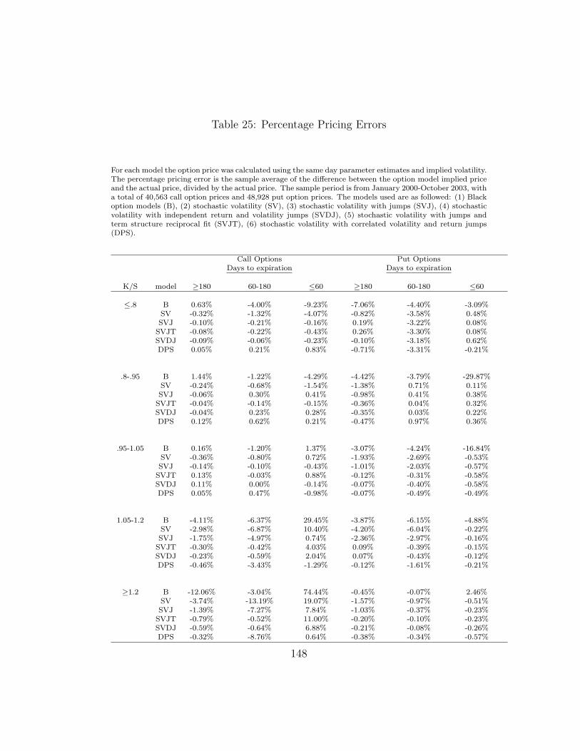
Table 25: Percentage Pricing Errors
For each model the option price was calculated using the same day parameter estimates and implied volatility.The percentage pricing error is the sample average of the difference between the option model implied priceand the actual price, divided by the actual price. The sample period is from January 2000-October 2003, witha total of 40,563 call option prices and 48,928 put option prices. The models used are as followed: (1) Blackoption models (B), (2) stochastic volatility (SV), (3) stochastic volatility with jumps (SVJ), (4) stochasticvolatility with independent return and volatility jumps (SVDJ), (5) stochastic volatility with jumps andterm structure reciprocal fit (SVJT), (6) stochastic volatility with correlated volatility and return jumps(DPS).
Call Options Put OptionsDays to expiration Days to expiration
K/S model ≥180 60-180 ≤60 ≥180 60-180 ≤60
≤.8 B 0.63% -4.00% -9.23% -7.06% -4.40% -3.09%SV -0.32% -1.32% -4.07% -0.82% -3.58% 0.48%SVJ -0.10% -0.21% -0.16% 0.19% -3.22% 0.08%
SVJT -0.08% -0.22% -0.43% 0.26% -3.30% 0.08%SVDJ -0.09% -0.06% -0.23% -0.10% -3.18% 0.62%DPS 0.05% 0.21% 0.83% -0.71% -3.31% -0.21%
.8-.95 B 1.44% -1.22% -4.29% -4.42% -3.79% -29.87%SV -0.24% -0.68% -1.54% -1.38% 0.71% 0.11%SVJ -0.06% 0.30% 0.41% -0.98% 0.41% 0.38%
SVJT -0.04% -0.14% -0.15% -0.36% 0.04% 0.32%SVDJ -0.04% 0.23% 0.28% -0.35% 0.03% 0.22%DPS 0.12% 0.62% 0.21% -0.47% 0.97% 0.36%
.95-1.05 B 0.16% -1.20% 1.37% -3.07% -4.24% -16.84%SV -0.36% -0.80% 0.72% -1.93% -2.69% -0.53%SVJ -0.14% -0.10% -0.43% -1.01% -2.03% -0.57%
SVJT 0.13% -0.03% 0.88% -0.12% -0.31% -0.58%SVDJ 0.11% 0.00% -0.14% -0.07% -0.40% -0.58%DPS 0.05% 0.47% -0.98% -0.07% -0.49% -0.49%
1.05-1.2 B -4.11% -6.37% 29.45% -3.87% -6.15% -4.88%SV -2.98% -6.87% 10.40% -4.20% -6.04% -0.22%SVJ -1.75% -4.97% 0.74% -2.36% -2.97% -0.16%
SVJT -0.30% -0.42% 4.03% 0.09% -0.39% -0.15%SVDJ -0.23% -0.59% 2.04% 0.07% -0.43% -0.12%DPS -0.46% -3.43% -1.29% -0.12% -1.61% -0.21%
≥1.2 B -12.06% -3.04% 74.44% -0.45% -0.07% 2.46%SV -3.74% -13.19% 19.07% -1.57% -0.97% -0.51%SVJ -1.39% -7.27% 7.84% -1.03% -0.37% -0.23%
SVJT -0.79% -0.52% 11.00% -0.20% -0.10% -0.23%SVDJ -0.59% -0.64% 6.88% -0.21% -0.08% -0.26%DPS -0.32% -8.76% 0.64% -0.38% -0.34% -0.57%
148
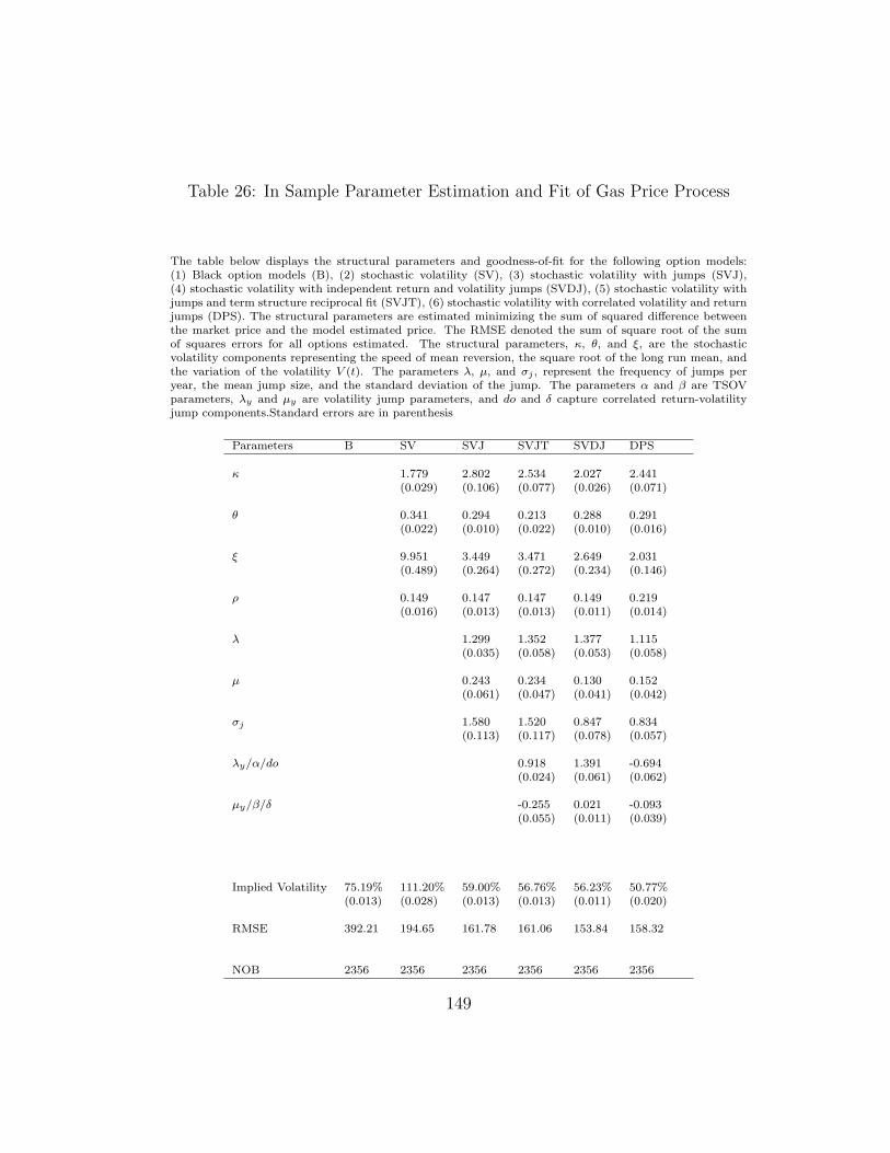
Table 26: In Sample Parameter Estimation and Fit of Gas Price Process
The table below displays the structural parameters and goodness-of-fit for the following option models:(1) Black option models (B), (2) stochastic volatility (SV), (3) stochastic volatility with jumps (SVJ),(4) stochastic volatility with independent return and volatility jumps (SVDJ), (5) stochastic volatility withjumps and term structure reciprocal fit (SVJT), (6) stochastic volatility with correlated volatility and returnjumps (DPS). The structural parameters are estimated minimizing the sum of squared difference betweenthe market price and the model estimated price. The RMSE denoted the sum of square root of the sumof squares errors for all options estimated. The structural parameters, κ, θ, and ξ, are the stochasticvolatility components representing the speed of mean reversion, the square root of the long run mean, andthe variation of the volatility V (t). The parameters λ, µ, and σj , represent the frequency of jumps peryear, the mean jump size, and the standard deviation of the jump. The parameters α and β are TSOVparameters, λy and µy are volatility jump parameters, and do and δ capture correlated return-volatilityjump components.Standard errors are in parenthesis
Parameters B SV SVJ SVJT SVDJ DPS
κ 1.779 2.802 2.534 2.027 2.441(0.029) (0.106) (0.077) (0.026) (0.071)
θ 0.341 0.294 0.213 0.288 0.291(0.022) (0.010) (0.022) (0.010) (0.016)
ξ 9.951 3.449 3.471 2.649 2.031(0.489) (0.264) (0.272) (0.234) (0.146)
ρ 0.149 0.147 0.147 0.149 0.219(0.016) (0.013) (0.013) (0.011) (0.014)
λ 1.299 1.352 1.377 1.115(0.035) (0.058) (0.053) (0.058)
µ 0.243 0.234 0.130 0.152(0.061) (0.047) (0.041) (0.042)
σj 1.580 1.520 0.847 0.834(0.113) (0.117) (0.078) (0.057)
λy/α/do 0.918 1.391 -0.694(0.024) (0.061) (0.062)
µy/β/δ -0.255 0.021 -0.093(0.055) (0.011) (0.039)
Implied Volatility 75.19% 111.20% 59.00% 56.76% 56.23% 50.77%(0.013) (0.028) (0.013) (0.013) (0.011) (0.020)
RMSE 392.21 194.65 161.78 161.06 153.84 158.32
NOB 2356 2356 2356 2356 2356 2356
149

Table 27: Parameter Estimation for BIV less than 50%
The table below displays the structural parameters and goodness-of-fit for the following option models forBlack implied volatility of less than 50%: (1) Black option models (B), (2) stochastic volatility (SV), (3)stochastic volatility with jumps (SVJ), (4) stochastic volatility with independent return and volatility jumps(SVDJ), (5) stochastic volatility with jumps and term structure reciprocal fit (SVJT), (6) stochastic volatilitywith correlated volatility and return jumps (DPS). The structural parameters are estimated minimizing thesum of squared difference between the market price and the model estimated price. The RMSE denoted thesum of square root of the sum of squares errors for all options estimated. The structural parameters, κ, θ,and ξ, are the stochastic volatility components representing the speed of mean reversion, the square rootof the long run mean, and the variation of the volatility V (t). The parameters λ, µ, and σj , represent thefrequency of jumps per year, the mean jump size, and the standard deviation of the jump. The parametersα and β are TSOV parameters, λy and µy are volatility jump parameters, and do and δ capture correlatedreturn-volatility jump components.Standard errors are in parenthesis
Parameters B SV SVJ SVJT SVDJ DPSκ 1.935 1.946 1.945 1.945 1.921
(0.011) (0.004) (0.003) (0.002) (0.007)
θ 0.304 0.318 0.307 0.315 0.269(0.005) (0.005) (0.004) (0.005) (0.004)
ξ 0.825 0.389 0.419 0.375 0.453(0.162) (0.015) (0.021) (0.014) (0.013)
ρ 0.376 0.256 0.249 0.270 0.329(0.023) (0.015) (0.015) (0.013) (0.017)
λ 1.106 1.108 1.063 0.970(0.033) (0.028) (0.018) (0.008)
µ 0.059 0.064 0.063 -0.036(0.010) (0.010) (0.010) (0.013)
σj 0.045 0.044 0.041 0.035(0.004) (0.004) (0.003) (0.002)
λy/α/do 1.004 1.007 -0.010(0.001) (0.004) (0.016)
µy/β/δ 0.017 0.009 0.002(0.004) (0.004) (0.009)
Implied Volatility 44.11% 48.45% 43.34% 42.43% 43.17% 39.50%(0.002) (0.007) (0.004) (0.004) (0.004) (0.003)
RMSE 7.92 4.65 4.35 4.35 4.32 4.41
NOB 716 716 716 716 716 716
150

Table 28: Parameter Estimation for BIV less than 80%
The table below displays the structural parameters and goodness-of-fit for the following option models forBlack implied volatility of less than 80%: (1) Black option models (B), (2) stochastic volatility (SV), (3)stochastic volatility with jumps (SVJ), (4) stochastic volatility with independent return and volatility jumps(SVDJ), (5) stochastic volatility with jumps and term structure reciprocal fit (SVJT), (6) stochastic volatilitywith correlated volatility and return jumps (DPS). The structural parameters are estimated minimizing thesum of squared difference between the market price and the model estimated price. The RMSE denoted thesum of square root of the sum of squares errors for all options estimated. The structural parameters, κ, θ,and ξ, are the stochastic volatility components representing the speed of mean reversion, the square rootof the long run mean, and the variation of the volatility V (t). The parameters λ, µ, and σj , represent thefrequency of jumps per year, the mean jump size, and the standard deviation of the jump. The parametersα and β are TSOV parameters, λy and µy are volatility jump parameters, and do and δ capture correlatedreturn-volatility jump components.Standard errors are in parenthesis
Parameters B SV SVJ SVJT SVDJ DPSκ 1.865 2.591 2.319 2.019 2.265
(0.018) (0.113) (0.072) (0.028) (0.059)
θ 0.311 0.316 0.256 0.304 0.244(0.010) (0.007) (0.015) (0.005) (0.005)
ξ 2.306 0.989 0.841 0.442 0.723(0.212) (0.112) (0.087) (0.021) (0.037)
ρ 0.234 0.186 0.186 0.189 0.200(0.017) (0.013) (0.013) (0.011) (0.015)
λ 1.121 1.127 1.113 0.947(0.016) (0.016) (0.011) (0.010)
µ 0.169 0.161 0.072 -0.041(0.028) (0.026) (0.010) (0.011)
σj 0.541 0.441 0.172 0.330(0.072) (0.064) (0.030) (0.043)
λy/α/do 0.939 1.113 -0.267(0.025) (0.030) (0.033)
µy/β/δ -0.200 0.009 0.049(0.057) (0.005) (0.026)
Implied Volatility 53.61% 65.00% 54.04% 52.43% 51.08% 46.73%(0.002) (0.010) (0.010) (0.009) (0.005) (0.007)
RMSE 157.11 120.06 107.68 108.02 104.50 107.77
NOB 1877 1877 1877 1877 1877 1877
151

Table 29: Parameter Estimation for BIV less than 100%
The table below displays the structural parameters and goodness-of-fit for the following option models forBlack implied volatility of less than 100%: (1) Black option models (B), (2) stochastic volatility (SV), (3)stochastic volatility with jumps (SVJ), (4) stochastic volatility with independent return and volatility jumps(SVDJ), (5) stochastic volatility with jumps and term structure reciprocal fit (SVJT), (6) stochastic volatilitywith correlated volatility and return jumps (DPS). The structural parameters are estimated minimizing thesum of squared difference between the market price and the model estimated price. The RMSE denoted thesum of square root of the sum of squares errors for all options estimated. The structural parameters, κ, θ,and ξ, are the stochastic volatility components representing the speed of mean reversion, the square rootof the long run mean, and the variation of the volatility V (t). The parameters λ, µ, and σj , represent thefrequency of jumps per year, the mean jump size, and the standard deviation of the jump. The parametersα and β are TSOV parameters, λy and µy are volatility jump parameters, and do and δ capture correlatedreturn-volatility jump components.Standard errors are in parenthesis
Parameters B SV SVJ SVJT SVDJ DPSκ 1.835 2.782 2.510 2.025 2.374
(0.019) (0.117) (0.084) (0.026) (0.062)
θ 0.305 0.303 0.230 0.295 0.242(0.010) (0.006) (0.023) (0.005) (0.005)
ξ 2.798 1.153 1.011 0.488 0.929(0.217) (0.117) (0.095) (0.023) (0.052)
ρ 0.192 0.177 0.173 0.164 0.193(0.017) (0.013) (0.013) (0.011) (0.015)
λ 1.139 1.134 1.144 0.943(0.018) (0.015) (0.015) (0.009)
µ 0.172 0.171 0.081 0.013(0.027) (0.026) (0.012) (0.041)
σj 0.768 0.654 0.221 0.403(0.080) (0.071) (0.029) (0.045)
λy/α/do 0.908 1.151 -0.347(0.027) (0.031) (0.037)
µy/β/δ -0.257 0.006 0.041(0.062) (0.004) (0.034)
Implied Volatility 56.15% 70.54% 54.39% 53.07% 51.70% 47.96%(0.003) (0.011) (0.010) (0.009) (0.006) (0.007)
RMSE 222.69 168.18 146.67 147.17 142.15 146.83
NOB 2029 2029 2029 2029 2029 2029
152
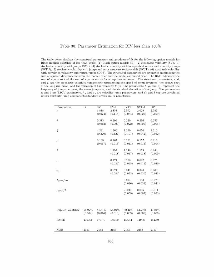
Table 30: Parameter Estimation for BIV less than 150%
The table below displays the structural parameters and goodness-of-fit for the following option models forBlack implied volatility of less than 150%: (1) Black option models (B), (2) stochastic volatility (SV), (3)stochastic volatility with jumps (SVJ), (4) stochastic volatility with independent return and volatility jumps(SVDJ), (5) stochastic volatility with jumps and term structure reciprocal fit (SVJT), (6) stochastic volatilitywith correlated volatility and return jumps (DPS). The structural parameters are estimated minimizing thesum of squared difference between the market price and the model estimated price. The RMSE denoted thesum of square root of the sum of squares errors for all options estimated. The structural parameters, κ, θ,and ξ, are the stochastic volatility components representing the speed of mean reversion, the square rootof the long run mean, and the variation of the volatility V (t). The parameters λ, µ, and σj , represent thefrequency of jumps per year, the mean jump size, and the standard deviation of the jump. The parametersα and β are TSOV parameters, λy and µy are volatility jump parameters, and do and δ capture correlatedreturn-volatility jump components.Standard errors are in parenthesis
Parameters B SV SVJ SVJT SVDJ DPSκ 1.818 2.858 2.572 2.029 2.387
(0.024) (0.116) (0.084) (0.027) (0.059)
θ 0.313 0.309 0.220 0.296 0.256(0.012) (0.009) (0.022) (0.009) (0.005)
ξ 4.291 1.366 1.190 0.650 1.010(0.270) (0.127) (0.107) (0.042) (0.052)
ρ 0.169 0.167 0.162 0.157 0.216(0.017) (0.013) (0.013) (0.011) (0.014)
λ 1.157 1.148 1.179 0.943(0.018) (0.017) (0.018) (0.009)
µ 0.171 0.168 0.092 0.075(0.026) (0.025) (0.014) (0.040)
σj 0.971 0.841 0.328 0.468(0.084) (0.073) (0.030) (0.043)
λy/α/do 0.914 1.184 -0.478(0.026) (0.033) (0.041)
µy/β/δ -0.244 0.006 -0.011(0.059) (0.007) (0.033)
Implied Volatility 59.92% 81.61% 54.04% 52.42% 51.27% 47.81%(0.004) (0.016) (0.010) (0.009) (0.006) (0.006)
RMSE 270.53 179.70 155.09 155.44 149.89 154.60
NOB 2153 2153 2153 2153 2153 2153
153

Table 31: Parameter Estimation for BIV less than 200%
The table below displays the structural parameters and goodness-of-fit for the following option models forBlack implied volatility of less than 200%: (1) Black option models (B), (2) stochastic volatility (SV), (3)stochastic volatility with jumps (SVJ), (4) stochastic volatility with independent return and volatility jumps(SVDJ), (5) stochastic volatility with jumps and term structure reciprocal fit (SVJT), (6) stochastic volatilitywith correlated volatility and return jumps (DPS). The structural parameters are estimated minimizing thesum of squared difference between the market price and the model estimated price. The RMSE denoted thesum of square root of the sum of squares errors for all options estimated. The structural parameters, κ, θ,and ξ, are the stochastic volatility components representing the speed of mean reversion, the square rootof the long run mean, and the variation of the volatility V (t). The parameters λ, µ, and σj , represent thefrequency of jumps per year, the mean jump size, and the standard deviation of the jump. The parametersα and β are TSOV parameters, λy and µy are volatility jump parameters, and do and δ capture correlatedreturn-volatility jump components.Standard errors are in parenthesis
Parameters B SV SVJ SVJT SVDJ DPSκ 1.801 2.834 2.558 2.023 2.392
(0.030) (0.111) (0.081) (0.026) (0.057)
θ 0.321 0.304 0.224 0.296 0.270(0.012) (0.010) (0.023) (0.010) (0.006)
ξ 6.684 1.708 1.608 1.014 1.225(0.381) (0.143) (0.132) (0.091) (0.069)
ρ 0.149 0.150 0.149 0.147 0.222(0.016) (0.013) (0.013) (0.011) (0.014)
λ 1.213 1.266 1.286 0.965(0.032) (0.058) (0.053) (0.010)
µ 0.207 0.203 0.111 0.115(0.030) (0.028) (0.016) (0.039)
σj 1.206 1.091 0.511 0.600(0.095) (0.087) (0.053) (0.047)
λy/α/do 0.915 1.232 -0.647(0.025) (0.034) (0.047)
µy/β/δ -0.248 0.017 -0.056(0.058) (0.010) (0.033)
Implied Volatility 64.29% 96.25% 54.06% 52.86% 51.66% 47.70%(0.006) (0.024) (0.011) (0.011) (0.008) (0.006)
RMSE 315.23 184.85 157.32 157.55 150.69 155.72
NOB 2240 2240 2240 2240 2240 2240
154

Table 32: Parameter Estimation for BIV less than 300%
The table below displays the structural parameters and goodness-of-fit for the following option models forBlack implied volatility of less than 300%: (1) Black option models (B), (2) stochastic volatility (SV), (3)stochastic volatility with jumps (SVJ), (4) stochastic volatility with independent return and volatility jumps(SVDJ), (5) stochastic volatility with jumps and term structure reciprocal fit (SVJT), (6) stochastic volatilitywith correlated volatility and return jumps (DPS). The structural parameters are estimated minimizing thesum of squared difference between the market price and the model estimated price. The RMSE denoted thesum of square root of the sum of squares errors for all options estimated. The structural parameters, κ, θ,and ξ, are the stochastic volatility components representing the speed of mean reversion, the square rootof the long run mean, and the variation of the volatility V (t). The parameters λ, µ, and σj , represent thefrequency of jumps per year, the mean jump size, and the standard deviation of the jump. The parametersα and β are TSOV parameters, λy and µy are volatility jump parameters, and do and δ capture correlatedreturn-volatility jump components.Standard errors are in parenthesis
Parameters B SV SVJ SVJT SVDJ DPSκ 1.782 2.805 2.542 2.014 2.387
(0.029) (0.108) (0.078) (0.026) (0.056)
θ 0.318 0.296 0.218 0.293 0.272(0.012) (0.010) (0.023) (0.010) (0.006)
ξ 8.698 2.300 2.243 1.520 1.518(0.456) (0.183) (0.179) (0.139) (0.091)
ρ 0.143 0.141 0.140 0.143 0.221(0.016) (0.013) (0.013) (0.011) (0.014)
λ 1.264 1.314 1.340 1.011(0.033) (0.058) (0.052) (0.014)
µ 0.226 0.242 0.134 0.147(0.030) (0.030) (0.017) (0.039)
σj 1.493 1.445 0.745 0.760(0.111) (0.116) (0.072) (0.054)
λy/α/do 0.916 1.353 -0.749(0.024) (0.055) (0.051)
µy/β/δ -0.246 0.016 -0.094(0.056) (0.010) (0.034)
Implied Volatility 69.31% 105.79% 54.70% 53.19% 52.27% 47.75%(0.009) (0.027) (0.011) (0.011) (0.009) (0.006)
RMSE 359.97 191.78 160.39 160.61 152.57 157.66
NOB 2302 2302 2302 2302 2302 2302
155
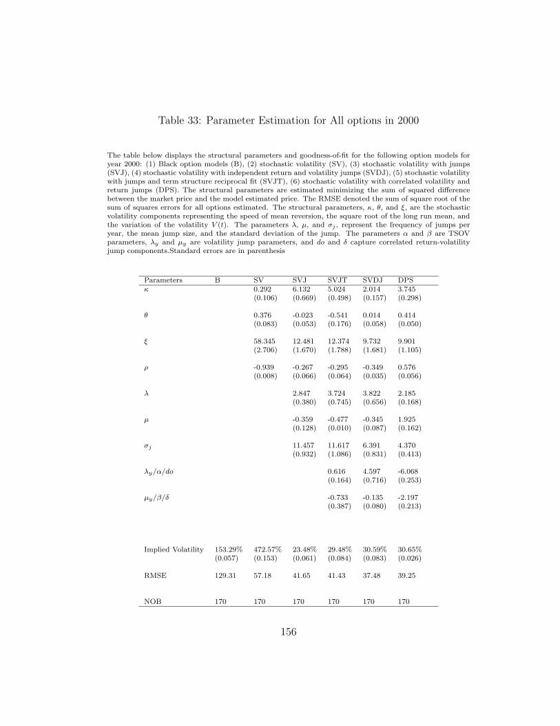
Table 33: Parameter Estimation for All options in 2000
The table below displays the structural parameters and goodness-of-fit for the following option models foryear 2000: (1) Black option models (B), (2) stochastic volatility (SV), (3) stochastic volatility with jumps(SVJ), (4) stochastic volatility with independent return and volatility jumps (SVDJ), (5) stochastic volatilitywith jumps and term structure reciprocal fit (SVJT), (6) stochastic volatility with correlated volatility andreturn jumps (DPS). The structural parameters are estimated minimizing the sum of squared differencebetween the market price and the model estimated price. The RMSE denoted the sum of square root of thesum of squares errors for all options estimated. The structural parameters, κ, θ, and ξ, are the stochasticvolatility components representing the speed of mean reversion, the square root of the long run mean, andthe variation of the volatility V (t). The parameters λ, µ, and σj , represent the frequency of jumps peryear, the mean jump size, and the standard deviation of the jump. The parameters α and β are TSOVparameters, λy and µy are volatility jump parameters, and do and δ capture correlated return-volatilityjump components.Standard errors are in parenthesis
Parameters B SV SVJ SVJT SVDJ DPSκ 0.292 6.132 5.024 2.014 3.745
(0.106) (0.669) (0.498) (0.157) (0.298)
θ 0.376 -0.023 -0.541 0.014 0.414(0.083) (0.053) (0.176) (0.058) (0.050)
ξ 58.345 12.481 12.374 9.732 9.901(2.706) (1.670) (1.788) (1.681) (1.105)
ρ -0.939 -0.267 -0.295 -0.349 0.576(0.008) (0.066) (0.064) (0.035) (0.056)
λ 2.847 3.724 3.822 2.185(0.380) (0.745) (0.656) (0.168)
µ -0.359 -0.477 -0.345 1.925(0.128) (0.010) (0.087) (0.162)
σj 11.457 11.617 6.391 4.370(0.932) (1.086) (0.831) (0.413)
λy/α/do 0.616 4.597 -6.068(0.164) (0.716) (0.253)
µy/β/δ -0.733 -0.135 -2.197(0.387) (0.080) (0.213)
Implied Volatility 153.29% 472.57% 23.48% 29.48% 30.59% 30.65%(0.057) (0.153) (0.061) (0.084) (0.083) (0.026)
RMSE 129.31 57.18 41.65 41.43 37.48 39.25
NOB 170 170 170 170 170 170
156

Table 34: Parameter Estimation for All options in 2001
The table below displays the structural parameters and goodness-of-fit for the following option models foryear 2001: (1) Black option models (B), (2) stochastic volatility (SV), (3) stochastic volatility with jumps(SVJ), (4) stochastic volatility with independent return and volatility jumps (SVDJ), (5) stochastic volatilitywith jumps and term structure reciprocal fit (SVJT), (6) stochastic volatility with correlated volatility andreturn jumps (DPS). The structural parameters are estimated minimizing the sum of squared differencebetween the market price and the model estimated price. The RMSE denoted the sum of square root of thesum of squares errors for all options estimated. The structural parameters, κ, θ, and ξ, are the stochasticvolatility components representing the speed of mean reversion, the square root of the long run mean, andthe variation of the volatility V (t). The parameters λ, µ, and σj , represent the frequency of jumps peryear, the mean jump size, and the standard deviation of the jump. The parameters α and β are TSOVparameters, λy and µy are volatility jump parameters, and do and δ capture correlated return-volatilityjump components.Standard errors are in parenthesis
Parameters B SV SVJ SVJT SVDJ DPSκ 1.851 3.072 2.693 2.089 2.562
(0.054) (0.187) (0.134) (0.048) (0.101)
θ 0.351 0.295 0.225 0.292 0.239(0.042) (0.016) (0.036) (0.018) (0.009)
ξ 10.602 4.720 4.733 3.637 2.159(0.646) (0.456) (0.464) (0.393) (0.208)
ρ 0.309 0.183 0.184 0.200 0.245(0.021) (0.019) (0.019) (0.016) (0.020)
λ 1.199 1.194 1.241 0.896(0.033) (0.032) (0.033) (0.018)
µ 0.620 0.603 0.518 0.096(0.114) (0.085) (0.080) (0.071)
σj 1.323 1.158 0.667 0.919(0.120) (0.102) (0.063) (0.075)
λy/α/do 0.878 1.253 -0.546(0.042) (0.054) (0.066)
µy/β/δ -0.419 0.053 0.127(0.095) (0.017) (0.054)
Implied Volatility 81.46% 102.70% 59.88% 56.12% 57.63% 48.44%(0.021) (0.028) (0.020) (0.018) (0.018) (0.008)
RMSE 251.07 129.46 113.49 113.96 110.13 112.90
NOB 1156 1156 1156 1156 1156 1156
157

Table 35: Parameter Estimation for All options in 2002
The table below displays the structural parameters and goodness-of-fit for the following option models foryear 2002: (1) Black option models (B), (2) stochastic volatility (SV), (3) stochastic volatility with jumps(SVJ), (4) stochastic volatility with independent return and volatility jumps (SVDJ), (5) stochastic volatilitywith jumps and term structure reciprocal fit (SVJT), (6) stochastic volatility with correlated volatility andreturn jumps (DPS). The structural parameters are estimated minimizing the sum of squared differencebetween the market price and the model estimated price. The RMSE denoted the sum of square root of thesum of squares errors for all options estimated. The structural parameters, κ, θ, and ξ, are the stochasticvolatility components representing the speed of mean reversion, the square root of the long run mean, andthe variation of the volatility V (t). The parameters λ, µ, and σj , represent the frequency of jumps peryear, the mean jump size, and the standard deviation of the jump. The parameters α and β are TSOVparameters, λy and µy are volatility jump parameters, and do and δ capture correlated return-volatilityjump components.Standard errors are in parenthesis
Parameters B SV SVJ SVJT SVDJ DPSκ 1.938 1.939 1.935 1.953 1.946
(0.014) (0.005) (0.005) (0.005) (0.007)
θ 0.324 0.358 0.328 0.333 0.294(0.006) (0.013) (0.007) (0.005) (0.004)
ξ 1.355 0.575 0.651 0.351 0.403(0.335) (0.068) (0.098) (0.033) (0.021)
ρ -0.004 0.144 0.149 0.131 0.013(0.029) (0.021) (0.021) (0.019) (0.022)
λ 1.193 1.174 1.151 1.018(0.031) (0.021) (0.030) (0.020)
µ 0.216 0.208 0.008 -0.082(0.066) (0.062) (0.023) (0.014)
σj 0.302 0.320 0.162 0.137(0.115) (0.120) (0.067) (0.049)
λy/α/do 1.011 1.016 -0.190(0.002) (0.010) (0.046)
µy/β/δ 0.009 0.006 -0.020(0.023) (0.009) (0.017)
Implied Volatility 59.43% 65.56% 70.97% 68.59% 64.43% 56.40%(0.004) (0.013) (0.023) (0.021) (0.009) (0.015)
RMSE 9.94 7.33 6.04 6.06 5.71 6.06
NOB 770 770 770 770 770 770
158

Table 36: Parameter Estimation for All options in 2003
The table below displays the structural parameters and goodness-of-fit for the following option models foryear 2003: (1) Black option models (B), (2) stochastic volatility (SV), (3) stochastic volatility with jumps(SVJ), (4) stochastic volatility with independent return and volatility jumps (SVDJ), (5) stochastic volatilitywith jumps and term structure reciprocal fit (SVJT), (6) stochastic volatility with correlated volatility andreturn jumps (DPS). The structural parameters are estimated minimizing the sum of squared differencebetween the market price and the model estimated price. The RMSE denoted the sum of square root of thesum of squares errors for all options estimated. The structural parameters, κ, θ, and ξ, are the stochasticvolatility components representing the speed of mean reversion, the square root of the long run mean, andthe variation of the volatility V (t). The parameters λ, µ, and σj , represent the frequency of jumps peryear, the mean jump size, and the standard deviation of the jump. The parameters α and β are TSOVparameters, λy and µy are volatility jump parameters, and do and δ capture correlated return-volatilityjump components.Standard errors are in parenthesis
Parameters B SV SVJ SVJT SVDJ DPSκ 1.956 1.945 1.943 1.943 1.940
(0.005) (0.002) (0.002) (0.002) (0.001)
θ 0.320 0.313 0.309 0.316 0.271(0.002) (0.003) (0.003) (0.004) (0.002)
ξ 0.387 0.381 0.381 0.383 0.450(0.010) (0.012) (0.012) (0.012) (0.006)
ρ 0.634 0.288 0.289 0.308 0.493(0.020) (0.006) (0.006) (0.006) (0.016)
λ 1.001 0.993 0.998 0.959(0.002) (0.002) (0.002) (0.004)
µ 0.141 0.145 0.142 -0.045(0.006) (0.006) (0.006) (0.005)
σj 0.026 0.025 0.024 0.027(0.001) (0.001) (0.001) (0.001)
λy/α/do 0.999 0.997 0.116(0.001) (0.001) (0.005)
µy/β/δ 0.004 0.018 0.006(0.001) (0.003) (0.001)
Implied Volatility 41.15% 43.57% 41.47% 41.61% 40.72% 38.26%(0.004) (0.005) (0.006) (0.006) (0.006) (0.005)
RMSE 0.36 0.01 0.01 0.01 0.01 0.01
NOB 252 252 252 252 252 252
159

Table 37: Parameter Estimation for Long-Term Options
The table below displays the structural parameters and goodness-of-fit for the following option models foroptions with 180 days or more until expiration: (1) Black option models (B), (2) stochastic volatility (SV), (3)stochastic volatility with jumps (SVJ), (4) stochastic volatility with independent return and volatility jumps(SVDJ), (5) stochastic volatility with jumps and term structure reciprocal fit (SVJT), (6) stochastic volatilitywith correlated volatility and return jumps (DPS). The structural parameters are estimated minimizing thesum of squared difference between the market price and the model estimated price. The RMSE denoted thesum of square root of the sum of squares errors for all options estimated. The structural parameters, κ, θ,and ξ, are the stochastic volatility components representing the speed of mean reversion, the square rootof the long run mean, and the variation of the volatility V (t). The parameters λ, µ, and σj , represent thefrequency of jumps per year, the mean jump size, and the standard deviation of the jump. The parametersα and β are TSOV parameters, λy and µy are volatility jump parameters, and do and δ capture correlatedreturn-volatility jump components.Standard errors are in parenthesis
Parameters B SV SVJ SVJT SVDJ DPSκ 1.891 2.914 2.449 2.118 2.324
(0.036) (0.202) (0.117) (0.076) (0.097)
θ 0.347 0.313 0.237 0.306 0.250(0.017) (0.005) (0.023) (0.005) (0.008)
ξ 1.770 1.061 0.850 0.400 0.654(0.264) (0.216) (0.194) (0.031) (0.071)
ρ 0.563 0.319 0.314 0.331 0.454(0.017) (0.014) (0.014) (0.008) (0.015)
λ 0.952 0.949 0.987 0.901(0.007) (0.007) (0.006) (0.007)
µ 0.126 0.139 0.138 -0.029(0.010) (0.011) (0.010) (0.016)
σj 0.480 0.299 0.132 0.240(0.091) (0.056) (0.022) (0.044)
λy/α/do 0.896 1.094 -0.122(0.064) (0.039) (0.039)
µy/β/δ -0.278 -0.005 0.185(0.110) (0.002) (0.065)
Implied Volatility 48.60% 58.13% 46.94% 46.90% 46.48% 43.18%(0.003) (0.011) (0.007) (0.007) (0.007) (0.006)
RMSE 51.00 41.56 36.62 36.92 35.66 36.76
NOB 654 654 654 654 654 654
160

Table 38: Parameter Estimation for Medium-Term Options
The table below displays the structural parameters and goodness-of-fit for the following option models foroptions expiring between 60 and 180 days: (1) Black option models (B), (2) stochastic volatility (SV), (3)stochastic volatility with jumps (SVJ), (4) stochastic volatility with independent return and volatility jumps(SVDJ), (5) stochastic volatility with jumps and term structure reciprocal fit (SVJT), (6) stochastic volatilitywith correlated volatility and return jumps (DPS). The structural parameters are estimated minimizing thesum of squared difference between the market price and the model estimated price. The RMSE denoted thesum of square root of the sum of squares errors for all options estimated. The structural parameters, κ, θ,and ξ, are the stochastic volatility components representing the speed of mean reversion, the square rootof the long run mean, and the variation of the volatility V (t). The parameters λ, µ, and σj , represent thefrequency of jumps per year, the mean jump size, and the standard deviation of the jump. The parametersα and β are TSOV parameters, λy and µy are volatility jump parameters, and do and δ capture correlatedreturn-volatility jump components.Standard errors are in parenthesis
Parameters B SV SVJ SVJT SVDJ DPSκ 1.747 3.029 2.776 1.996 2.533
(0.036) (0.171) (0.132) (0.024) (0.090)
θ 0.325 0.276 0.204 0.279 0.251(0.018) (0.008) (0.036) (0.008) (0.008)
ξ 6.257 1.526 1.228 0.753 1.403(0.485) (0.186) (0.132) (0.083) (0.103)
ρ 0.004 0.096 0.098 0.075 0.130(0.023) (0.018) (0.018) (0.015) (0.020)
λ 1.144 1.150 1.192 0.964(0.015) (0.017) (0.014) (0.014)
µ 0.048 0.046 0.029 0.119(0.021) (0.021) (0.020) (0.024)
σj 1.345 1.187 0.488 0.667(0.140) (0.122) (0.081) (0.071)
λy/α/do 0.902 1.290 -0.712(0.030) (0.054) (0.061)
µy/β/δ -0.278 -0.006 -0.147(0.084) (0.006) (0.042)
Implied Volatility 64.38% 100.66% 50.82% 49.91% 51.08% 48.67%(0.006) (0.034) (0.008) (0.008) (0.008) (0.010)
RMSE 207.09 131.99 113.15 113.23 108.77 112.23
NOB 1231 1231 1231 1231 1231 1231
161
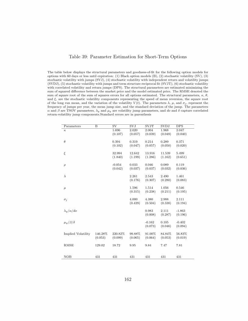
Table 39: Parameter Estimation for Short-Term Options
The table below displays the structural parameters and goodness-of-fit for the following option models foroptions with 60 days or less until expiration: (1) Black option models (B), (2) stochastic volatility (SV), (3)stochastic volatility with jumps (SVJ), (4) stochastic volatility with independent return and volatility jumps(SVDJ), (5) stochastic volatility with jumps and term structure reciprocal fit (SVJT), (6) stochastic volatilitywith correlated volatility and return jumps (DPS). The structural parameters are estimated minimizing thesum of squared difference between the market price and the model estimated price. The RMSE denoted thesum of square root of the sum of squares errors for all options estimated. The structural parameters, κ, θ,and ξ, are the stochastic volatility components representing the speed of mean reversion, the square rootof the long run mean, and the variation of the volatility V (t). The parameters λ, µ, and σj , represent thefrequency of jumps per year, the mean jump size, and the standard deviation of the jump. The parametersα and β are TSOV parameters, λy and µy are volatility jump parameters, and do and δ capture correlatedreturn-volatility jump components.Standard errors are in parenthesis
Parameters B SV SVJ SVJT SVDJ DPSκ 1.696 2.020 2.004 1.968 2.047
(0.107) (0.057) (0.039) (0.049) (0.040)
θ 0.394 0.319 0.214 0.289 0.371(0.102) (0.047) (0.057) (0.050) (0.020)
ξ 32.994 12.642 13.916 11.539 5.499(1.840) (1.199) (1.286) (1.162) (0.651)
ρ -0.054 0.033 0.046 0.089 0.119(0.042) (0.037) (0.037) (0.032) (0.036)
λ 2.261 2.543 2.490 1.461(0.176) (0.307) (0.280) (0.083)
µ 1.596 1.514 1.056 0.546(0.315) (0.238) (0.211) (0.195)
σj 4.000 4.380 2.988 2.111(0.429) (0.504) (0.338) (0.194)
λy/α/do 0.983 2.111 -1.863(0.008) (0.287) (0.196)
µy/β/δ -0.162 0.105 -0.402(0.073) (0.046) (0.094)
Implied Volatility 146.28% 220.82% 99.88% 91.00% 84.84% 56.83%(0.053) (0.099) (0.065) (0.064) (0.053) (0.019)
RMSE 129.02 18.72 9.95 9.84 7.47 7.81
NOB 431 431 431 431 431 431
162

Table 40: Parameter Estimation for Long-Term Options in the Winter Months
The table below displays the structural parameters and goodness-of-fit for the following option models forwinter options (December, January, and February) expiring in 180 days or more: (1) Black option models(B), (2) stochastic volatility (SV), (3) stochastic volatility with jumps (SVJ), (4) stochastic volatility withindependent return and volatility jumps (SVDJ), (5) stochastic volatility with jumps and term structurereciprocal fit (SVJT), (6) stochastic volatility with correlated volatility and return jumps (DPS). The struc-tural parameters are estimated minimizing the sum of squared difference between the market price and themodel estimated price. The RMSE denoted the sum of square root of the sum of squares errors for alloptions estimated. The structural parameters, κ, θ, and ξ, are the stochastic volatility components repre-senting the speed of mean reversion, the square root of the long run mean, and the variation of the volatilityV (t). The parameters λ, µ, and σj , represent the frequency of jumps per year, the mean jump size, and thestandard deviation of the jump. The parameters α and β are TSOV parameters, λy and µy are volatilityjump parameters, and do and δ capture correlated return-volatility jump components.Standard errors arein parenthesis
Parameters B SV SVJ SVJT SVDJ DPSκ 1.759 3.041 2.573 2.206 2.230
(0.039) (0.349) (0.221) (0.111) (0.098)
θ 0.466 0.349 0.250 0.329 0.243(0.046) (0.014) (0.053) (0.013) (0.015)
ξ 3.216 0.450 0.336 0.374 0.676(0.693) (0.093) (0.060) (0.100) (0.100)
ρ 0.695 0.418 0.402 0.370 0.644(0.036) (0.031) (0.032) (0.020) (0.027)
λ 0.922 0.929 0.973 0.828(0.019) (0.018) (0.016) (0.016)
µ 0.205 0.220 0.216 -0.087(0.022) (0.021) (0.017) (0.028)
σj 0.424 0.273 0.195 0.206(0.106) (0.059) (0.044) (0.042)
λy/α/do 0.973 1.199 -0.116(0.031) (0.114) (0.066)
µy/β/δ -0.034 -0.014 0.395(0.051) (0.006) (0.187)
Implied Volatility 57.89% 77.58% 58.47% 58.71% 58.29% 53.14%(0.003) (0.030) (0.015) (0.015) (0.015) (0.011)
RMSE 18.38 14.57 13.21 13.24 13.09 13.12
NOB 190 190 190 190 190 190
163
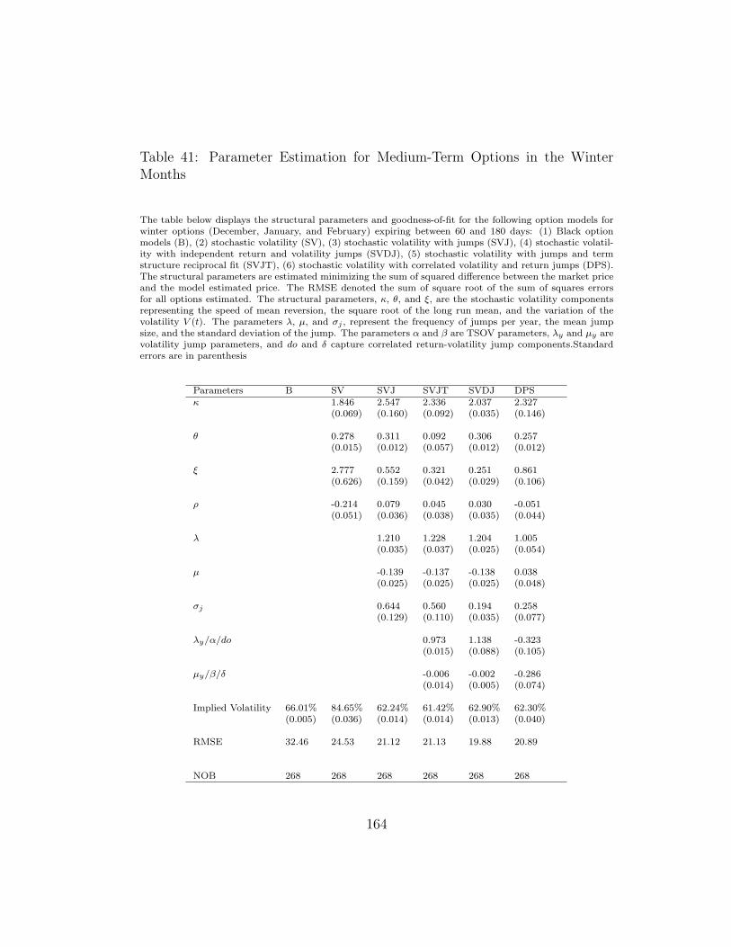
Table 41: Parameter Estimation for Medium-Term Options in the WinterMonths
The table below displays the structural parameters and goodness-of-fit for the following option models forwinter options (December, January, and February) expiring between 60 and 180 days: (1) Black optionmodels (B), (2) stochastic volatility (SV), (3) stochastic volatility with jumps (SVJ), (4) stochastic volatil-ity with independent return and volatility jumps (SVDJ), (5) stochastic volatility with jumps and termstructure reciprocal fit (SVJT), (6) stochastic volatility with correlated volatility and return jumps (DPS).The structural parameters are estimated minimizing the sum of squared difference between the market priceand the model estimated price. The RMSE denoted the sum of square root of the sum of squares errorsfor all options estimated. The structural parameters, κ, θ, and ξ, are the stochastic volatility componentsrepresenting the speed of mean reversion, the square root of the long run mean, and the variation of thevolatility V (t). The parameters λ, µ, and σj , represent the frequency of jumps per year, the mean jumpsize, and the standard deviation of the jump. The parameters α and β are TSOV parameters, λy and µy arevolatility jump parameters, and do and δ capture correlated return-volatility jump components.Standarderrors are in parenthesis
Parameters B SV SVJ SVJT SVDJ DPSκ 1.846 2.547 2.336 2.037 2.327
(0.069) (0.160) (0.092) (0.035) (0.146)
θ 0.278 0.311 0.092 0.306 0.257(0.015) (0.012) (0.057) (0.012) (0.012)
ξ 2.777 0.552 0.321 0.251 0.861(0.626) (0.159) (0.042) (0.029) (0.106)
ρ -0.214 0.079 0.045 0.030 -0.051(0.051) (0.036) (0.038) (0.035) (0.044)
λ 1.210 1.228 1.204 1.005(0.035) (0.037) (0.025) (0.054)
µ -0.139 -0.137 -0.138 0.038(0.025) (0.025) (0.025) (0.048)
σj 0.644 0.560 0.194 0.258(0.129) (0.110) (0.035) (0.077)
λy/α/do 0.973 1.138 -0.323(0.015) (0.088) (0.105)
µy/β/δ -0.006 -0.002 -0.286(0.014) (0.005) (0.074)
Implied Volatility 66.01% 84.65% 62.24% 61.42% 62.90% 62.30%(0.005) (0.036) (0.014) (0.014) (0.013) (0.040)
RMSE 32.46 24.53 21.12 21.13 19.88 20.89
NOB 268 268 268 268 268 268
164
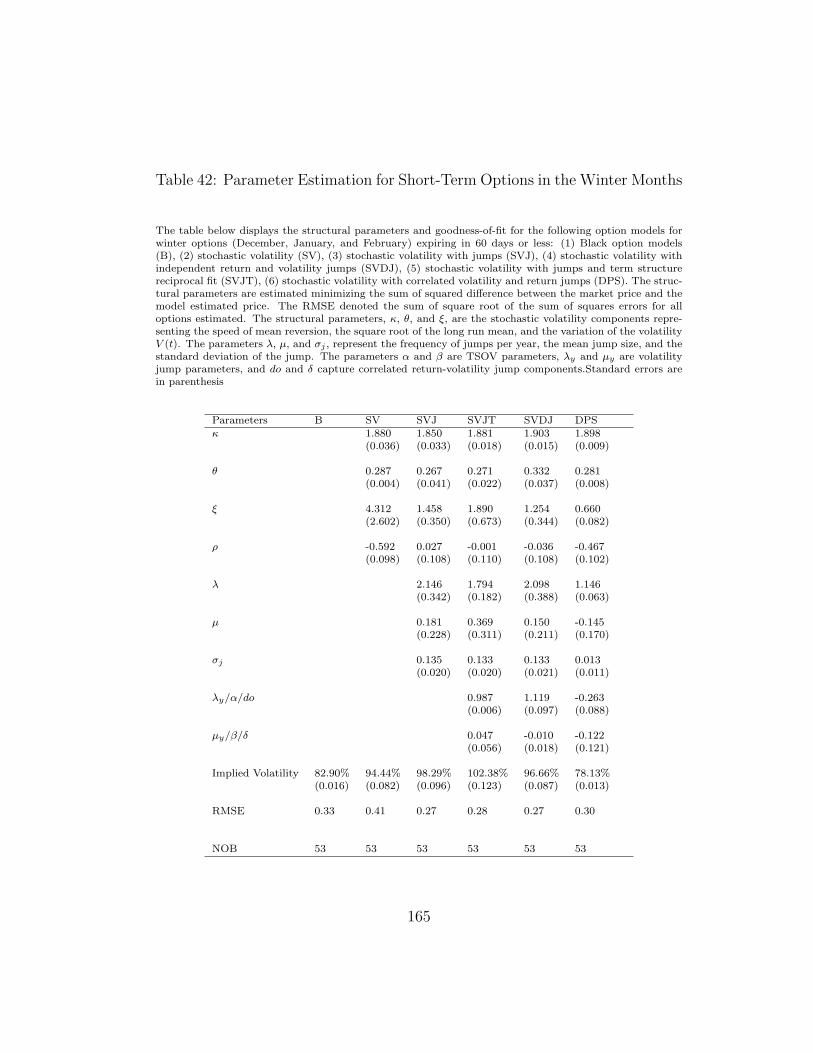
Table 42: Parameter Estimation for Short-Term Options in the Winter Months
The table below displays the structural parameters and goodness-of-fit for the following option models forwinter options (December, January, and February) expiring in 60 days or less: (1) Black option models(B), (2) stochastic volatility (SV), (3) stochastic volatility with jumps (SVJ), (4) stochastic volatility withindependent return and volatility jumps (SVDJ), (5) stochastic volatility with jumps and term structurereciprocal fit (SVJT), (6) stochastic volatility with correlated volatility and return jumps (DPS). The struc-tural parameters are estimated minimizing the sum of squared difference between the market price and themodel estimated price. The RMSE denoted the sum of square root of the sum of squares errors for alloptions estimated. The structural parameters, κ, θ, and ξ, are the stochastic volatility components repre-senting the speed of mean reversion, the square root of the long run mean, and the variation of the volatilityV (t). The parameters λ, µ, and σj , represent the frequency of jumps per year, the mean jump size, and thestandard deviation of the jump. The parameters α and β are TSOV parameters, λy and µy are volatilityjump parameters, and do and δ capture correlated return-volatility jump components.Standard errors arein parenthesis
Parameters B SV SVJ SVJT SVDJ DPSκ 1.880 1.850 1.881 1.903 1.898
(0.036) (0.033) (0.018) (0.015) (0.009)
θ 0.287 0.267 0.271 0.332 0.281(0.004) (0.041) (0.022) (0.037) (0.008)
ξ 4.312 1.458 1.890 1.254 0.660(2.602) (0.350) (0.673) (0.344) (0.082)
ρ -0.592 0.027 -0.001 -0.036 -0.467(0.098) (0.108) (0.110) (0.108) (0.102)
λ 2.146 1.794 2.098 1.146(0.342) (0.182) (0.388) (0.063)
µ 0.181 0.369 0.150 -0.145(0.228) (0.311) (0.211) (0.170)
σj 0.135 0.133 0.133 0.013(0.020) (0.020) (0.021) (0.011)
λy/α/do 0.987 1.119 -0.263(0.006) (0.097) (0.088)
µy/β/δ 0.047 -0.010 -0.122(0.056) (0.018) (0.121)
Implied Volatility 82.90% 94.44% 98.29% 102.38% 96.66% 78.13%(0.016) (0.082) (0.096) (0.123) (0.087) (0.013)
RMSE 0.33 0.41 0.27 0.28 0.27 0.30
NOB 53 53 53 53 53 53
165

Table 43: Parameter Estimation for Long-Term Options in the Spring Months
The table below displays the structural parameters and goodness-of-fit for the following option models forspring options (March, April, and May) expiring in 180 days or more: (1) Black option models (B), (2)stochastic volatility (SV), (3) stochastic volatility with jumps (SVJ), (4) stochastic volatility with indepen-dent return and volatility jumps (SVDJ), (5) stochastic volatility with jumps and term structure reciprocalfit (SVJT), (6) stochastic volatility with correlated volatility and return jumps (DPS). The structural pa-rameters are estimated minimizing the sum of squared difference between the market price and the modelestimated price. The RMSE denoted the sum of square root of the sum of squares errors for all optionsestimated. The structural parameters, κ, θ, and ξ, are the stochastic volatility components representingthe speed of mean reversion, the square root of the long run mean, and the variation of the volatility V (t).The parameters λ, µ, and σj , represent the frequency of jumps per year, the mean jump size, and thestandard deviation of the jump. The parameters α and β are TSOV parameters, λy and µy are volatilityjump parameters, and do and δ capture correlated return-volatility jump components.Standard errors arein parenthesis
Parameters B SV SVJ SVJT SVDJ DPSκ 1.921 1.941 1.931 1.935 1.935
(0.005) (0.003) (0.004) (0.004) (0.001)
θ 0.305 0.296 0.299 0.292 0.275(0.005) (0.005) (0.004) (0.005) (0.003)
ξ 0.587 0.460 0.467 0.466 0.465(0.036) (0.014) (0.015) (0.014) (0.008)
ρ 0.404 0.266 0.269 0.300 0.263(0.020) (0.017) (0.017) (0.010) (0.017)
λ 0.974 0.967 0.978 0.961(0.004) (0.006) (0.004) (0.005)
µ 0.077 0.081 0.086 0.007(0.008) (0.008) (0.007) (0.007)
σj 0.041 0.041 0.042 0.036(0.004) (0.004) (0.004) (0.003)
λy/α/do 0.998 0.997 0.050(0.002) (0.002) (0.006)
µy/β/δ 0.005 -0.010 0.006(0.002) (0.003) (0.003)
Implied Volatility 43.90% 49.27% 43.52% 42.99% 43.91% 41.01%(0.004) (0.005) (0.007) (0.007) (0.006) (0.006)
RMSE 0.41 0.06 0.06 0.06 0.06 0.05
NOB 247 247 247 247 247 247
166
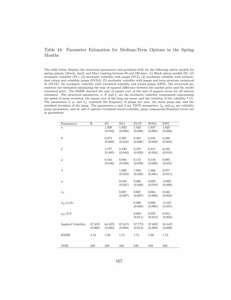
Table 44: Parameter Estimation for Medium-Term Options in the SpringMonths
The table below displays the structural parameters and goodness-of-fit for the following option models forspring options (March, April, and May) expiring between 60 and 180 days: (1) Black option models (B), (2)stochastic volatility (SV), (3) stochastic volatility with jumps (SVJ), (4) stochastic volatility with indepen-dent return and volatility jumps (SVDJ), (5) stochastic volatility with jumps and term structure reciprocalfit (SVJT), (6) stochastic volatility with correlated volatility and return jumps (DPS). The structural pa-rameters are estimated minimizing the sum of squared difference between the market price and the modelestimated price. The RMSE denoted the sum of square root of the sum of squares errors for all optionsestimated. The structural parameters, κ, θ, and ξ, are the stochastic volatility components representingthe speed of mean reversion, the square root of the long run mean, and the variation of the volatility V (t).The parameters λ, µ, and σj , represent the frequency of jumps per year, the mean jump size, and thestandard deviation of the jump. The parameters α and β are TSOV parameters, λy and µy are volatilityjump parameters, and do and δ capture correlated return-volatility jump components.Standard errors arein parenthesis
Parameters B SV SVJ SVJT SVDJ DPSκ 1.929 1.932 1.923 1.937 1.922
(0.016) (0.009) (0.008) (0.005) (0.006)
θ 0.275 0.307 0.304 0.316 0.289(0.008) (0.010) (0.006) (0.008) (0.005)
ξ 1.577 0.439 0.478 0.415 0.433(0.495) (0.034) (0.056) (0.034) (0.018)
ρ 0.162 0.094 0.115 0.140 0.085(0.036) (0.030) (0.029) (0.026) (0.031)
λ 1.099 1.093 1.086 0.977(0.018) (0.020) (0.021) (0.011)
µ 0.048 0.066 0.029 -0.062(0.021) (0.028) (0.019) (0.008)
σj 0.067 0.067 0.064 0.042(0.007) (0.007) (0.006) (0.004)
λy/α/do 0.999 0.998 -0.102(0.002) (0.005) (0.051)
µy/β/δ 0.004 0.025 0.012(0.011) (0.013) (0.003)
Implied Volatility 57.33% 64.33% 57.61% 57.77% 57.20% 52.44%(0.006) (0.020) (0.009) (0.013) (0.009) (0.008)
RMSE 4.44 1.98 1.71 1.71 1.69 1.73
NOB 348 348 348 348 348 348
167
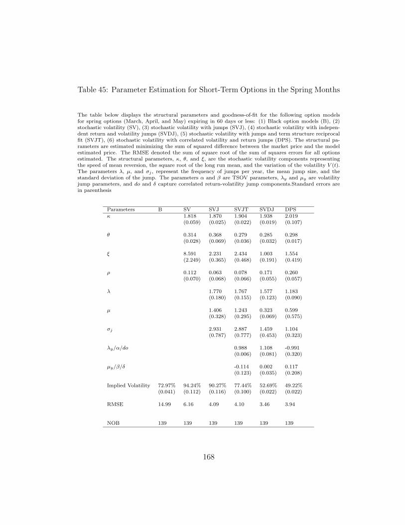
Table 45: Parameter Estimation for Short-Term Options in the Spring Months
The table below displays the structural parameters and goodness-of-fit for the following option modelsfor spring options (March, April, and May) expiring in 60 days or less: (1) Black option models (B), (2)stochastic volatility (SV), (3) stochastic volatility with jumps (SVJ), (4) stochastic volatility with indepen-dent return and volatility jumps (SVDJ), (5) stochastic volatility with jumps and term structure reciprocalfit (SVJT), (6) stochastic volatility with correlated volatility and return jumps (DPS). The structural pa-rameters are estimated minimizing the sum of squared difference between the market price and the modelestimated price. The RMSE denoted the sum of square root of the sum of squares errors for all optionsestimated. The structural parameters, κ, θ, and ξ, are the stochastic volatility components representingthe speed of mean reversion, the square root of the long run mean, and the variation of the volatility V (t).The parameters λ, µ, and σj , represent the frequency of jumps per year, the mean jump size, and thestandard deviation of the jump. The parameters α and β are TSOV parameters, λy and µy are volatilityjump parameters, and do and δ capture correlated return-volatility jump components.Standard errors arein parenthesis
Parameters B SV SVJ SVJT SVDJ DPSκ 1.818 1.870 1.904 1.938 2.019
(0.059) (0.025) (0.022) (0.019) (0.107)
θ 0.314 0.368 0.279 0.285 0.298(0.028) (0.069) (0.036) (0.032) (0.017)
ξ 8.591 2.231 2.434 1.003 1.554(2.249) (0.365) (0.468) (0.191) (0.419)
ρ 0.112 0.063 0.078 0.171 0.260(0.070) (0.068) (0.066) (0.055) (0.057)
λ 1.770 1.767 1.577 1.183(0.180) (0.155) (0.123) (0.090)
µ 1.406 1.243 0.323 0.599(0.328) (0.295) (0.069) (0.575)
σj 2.931 2.887 1.459 1.104(0.787) (0.777) (0.453) (0.323)
λy/α/do 0.988 1.108 -0.991(0.006) (0.081) (0.320)
µy/β/δ -0.114 0.002 0.117(0.123) (0.035) (0.208)
Implied Volatility 72.97% 94.24% 90.27% 77.44% 52.69% 49.22%(0.041) (0.112) (0.116) (0.100) (0.022) (0.022)
RMSE 14.99 6.16 4.09 4.10 3.46 3.94
NOB 139 139 139 139 139 139
168

Table 46: Parameter Estimation for Long-Term Options in the SummerMonths
The table below displays the structural parameters and goodness-of-fit for the following option models forsummer options (June, July, and August) expiring in 180 days or more: (1) Black option models (B), (2)stochastic volatility (SV), (3) stochastic volatility with jumps (SVJ), (4) stochastic volatility with indepen-dent return and volatility jumps (SVDJ), (5) stochastic volatility with jumps and term structure reciprocalfit (SVJT), (6) stochastic volatility with correlated volatility and return jumps (DPS). The structural pa-rameters are estimated minimizing the sum of squared difference between the market price and the modelestimated price. The RMSE denoted the sum of square root of the sum of squares errors for all optionsestimated. The structural parameters, κ, θ, and ξ, are the stochastic volatility components representingthe speed of mean reversion, the square root of the long run mean, and the variation of the volatility V (t).The parameters λ, µ, and σj , represent the frequency of jumps per year, the mean jump size, and thestandard deviation of the jump. The parameters α and β are TSOV parameters, λy and µy are volatilityjump parameters, and do and δ capture correlated return-volatility jump components.Standard errors arein parenthesis
Parameters B SV SVJ SVJT SVDJ DPSκ 1.942 1.963 1.957 1.956 1.941
(0.012) (0.006) (0.005) (0.005) (0.003)
θ 0.335 0.351 0.326 0.353 0.274(0.005) (0.007) (0.007) (0.008) (0.006)
ξ 0.496 0.257 0.247 0.235 0.375(0.156) (0.022) (0.022) (0.022) (0.013)
ρ 0.679 0.308 0.327 0.345 0.579(0.039) (0.025) (0.023) (0.014) (0.030)
λ 1.000 0.988 0.994 0.950(0.011) (0.007) (0.005) (0.009)
µ 0.111 0.118 0.129 -0.085(0.016) (0.016) (0.015) (0.013)
σj 0.042 0.039 0.032 0.038(0.008) (0.008) (0.006) (0.004)
λy/α/do 1.001 1.006 0.048(0.002) (0.009) (0.020)
µy/β/δ 0.010 0.024 0.018(0.004) (0.004) (0.004)
Implied Volatility 41.95% 44.48% 40.00% 40.43% 39.38% 37.53%(0.005) (0.014) (0.011) (0.011) (0.011) (0.010)
RMSE 1.10 0.82 0.79 0.79 0.77 0.78
NOB 146 146 146 146 146 146
169

Table 47: Parameter Estimation for Medium-Term Options in the SummerMonths
The table below displays the structural parameters and goodness-of-fit for the following option models forsummer options (June, July, and August) expiring between 60 and 180 days: (1) Black option models(B), (2) stochastic volatility (SV), (3) stochastic volatility with jumps (SVJ), (4) stochastic volatility withindependent return and volatility jumps (SVDJ), (5) stochastic volatility with jumps and term structurereciprocal fit (SVJT), (6) stochastic volatility with correlated volatility and return jumps (DPS). The struc-tural parameters are estimated minimizing the sum of squared difference between the market price and themodel estimated price. The RMSE denoted the sum of square root of the sum of squares errors for alloptions estimated. The structural parameters, κ, θ, and ξ, are the stochastic volatility components repre-senting the speed of mean reversion, the square root of the long run mean, and the variation of the volatilityV (t). The parameters λ, µ, and σj , represent the frequency of jumps per year, the mean jump size, and thestandard deviation of the jump. The parameters α and β are TSOV parameters, λy and µy are volatilityjump parameters, and do and δ capture correlated return-volatility jump components.Standard errors arein parenthesis
Parameters B SV SVJ SVJT SVDJ DPSκ 1.785 3.072 2.594 1.944 2.660
(0.079) (0.421) (0.197) (0.015) (0.192)
θ 0.365 0.304 0.257 0.288 0.271(0.042) (0.011) (0.022) (0.009) (0.016)
ξ 5.686 1.410 1.078 0.509 0.917(0.805) (0.425) (0.258) (0.071) (0.121)
ρ 0.215 0.207 0.202 0.180 0.355(0.042) (0.033) (0.032) (0.028) (0.033)
λ 1.110 1.086 1.148 0.957(0.027) (0.017) (0.022) (0.016)
µ 0.063 0.063 0.063 0.028(0.027) (0.029) (0.026) (0.032)
σj 1.204 1.082 0.299 0.861(0.228) (0.191) (0.043) (0.166)
λy/α/do 0.875 1.326 -0.802(0.057) (0.128) (0.124)
µy/β/δ -0.455 -0.023 0.032(0.209) (0.007) (0.096)
Implied Volatility 54.41% 84.08% 46.57% 44.93% 46.93% 39.79%(0.009) (0.049) (0.012) (0.010) (0.012) (0.008)
RMSE 49.95 31.28 25.54 25.60 24.55 25.35
NOB 354 354 354 354 354 354
170

Table 48: Parameter Estimation for Short-Term Options in the SummerMonths
The table below displays the structural parameters and goodness-of-fit for the following option models forsummer options (June, July, and August) expiring in 60 days or less: (1) Black option models (B), (2)stochastic volatility (SV), (3) stochastic volatility with jumps (SVJ), (4) stochastic volatility with indepen-dent return and volatility jumps (SVDJ), (5) stochastic volatility with jumps and term structure reciprocalfit (SVJT), (6) stochastic volatility with correlated volatility and return jumps (DPS). The structural pa-rameters are estimated minimizing the sum of squared difference between the market price and the modelestimated price. The RMSE denoted the sum of square root of the sum of squares errors for all optionsestimated. The structural parameters, κ, θ, and ξ, are the stochastic volatility components representingthe speed of mean reversion, the square root of the long run mean, and the variation of the volatility V (t).The parameters λ, µ, and σj , represent the frequency of jumps per year, the mean jump size, and thestandard deviation of the jump. The parameters α and β are TSOV parameters, λy and µy are volatilityjump parameters, and do and δ capture correlated return-volatility jump components.Standard errors arein parenthesis
Parameters B SV SVJ SVJT SVDJ DPSκ 0.975 1.780 1.929 1.619 2.006
(0.081) (0.067) (0.069) (0.056) (0.044)
θ 0.140 0.254 0.212 0.317 0.415(0.028) (0.120) (0.171) (0.131) (0.046)
ξ 50.159 11.787 14.113 11.076 7.356(3.529) (1.960) (2.221) (1.997) (1.244)
ρ -0.520 -0.246 -0.193 -0.147 0.175(0.069) (0.063) (0.064) (0.050) (0.073)
λ 2.996 3.437 3.333 2.414(0.211) (0.502) (0.278) (0.205)
µ 0.329 0.157 0.173 1.008(0.198) (0.114) (0.126) (0.172)
σj 7.413 8.617 5.522 3.365(1.004) (1.282) (0.837) (0.468)
λy/α/do 0.980 4.265 -4.437(0.022) (0.874) (0.392)
µy/β/δ 0.004 0.008 -1.210(0.158) (0.100) (0.179)
Implied Volatility 157.29% 337.69% 48.99% 47.16% 48.44% 34.71%(0.086) (0.213) (0.079) (0.084) (0.087) (0.022)
RMSE 59.40 10.37 4.59 4.68 3.21 3.20
NOB 136 136 136 136 136 136
171

Table 49: Parameter Estimation for Long-Term Options in the Fall Months
The table below displays the structural parameters and goodness-of-fit for the following option models forfall options (September, October, and November) expiring in 180 days or more: (1) Black option models(B), (2) stochastic volatility (SV), (3) stochastic volatility with jumps (SVJ), (4) stochastic volatility withindependent return and volatility jumps (SVDJ), (5) stochastic volatility with jumps and term structurereciprocal fit (SVJT), (6) stochastic volatility with correlated volatility and return jumps (DPS). The struc-tural parameters are estimated minimizing the sum of squared difference between the market price and themodel estimated price. The RMSE denoted the sum of square root of the sum of squares errors for alloptions estimated. The structural parameters, κ, θ, and ξ, are the stochastic volatility components repre-senting the speed of mean reversion, the square root of the long run mean, and the variation of the volatilityV (t). The parameters λ, µ, and σj , represent the frequency of jumps per year, the mean jump size, and thestandard deviation of the jump. The parameters α and β are TSOV parameters, λy and µy are volatilityjump parameters, and do and δ capture correlated return-volatility jump components.Standard errors arein parenthesis
Parameters B SV SVJ SVJT SVDJ DPSκ 1.949 7.591 4.736 2.739 4.527
(0.298) (1.416) (0.811) (0.605) (0.768)
θ 0.189 0.188 -0.191 0.192 0.128(0.084) (0.016) (0.137) (0.018) (0.059)
ξ 4.450 6.179 4.608 0.556 1.754(1.372) (1.781) (1.640) (0.072) (0.554)
ρ 0.507 0.253 0.203 0.288 0.338(0.034) (0.061) (0.061) (0.027) (0.054)
λ 0.820 0.826 0.997 0.753(0.033) (0.033) (0.033) (0.032)
µ 0.109 0.161 0.126 0.112(0.049) (0.064) (0.059) (0.116)
σj 2.937 1.732 0.466 1.401(0.695) (0.439) (0.155) (0.346)
λy/α/do 0.112 1.280 -1.044(0.551) (0.168) (0.275)
µy/β/δ -2.406 -0.024 0.563(0.929) (0.007) (0.299)
Implied Volatility 51.61% 62.35% 40.54% 40.46% 36.85% 34.30%(0.007) (0.031) (0.025) (0.032) (0.025) (0.024)
RMSE 31.11 26.12 22.56 22.83 21.74 22.80
NOB 74 74 74 74 74 74
172
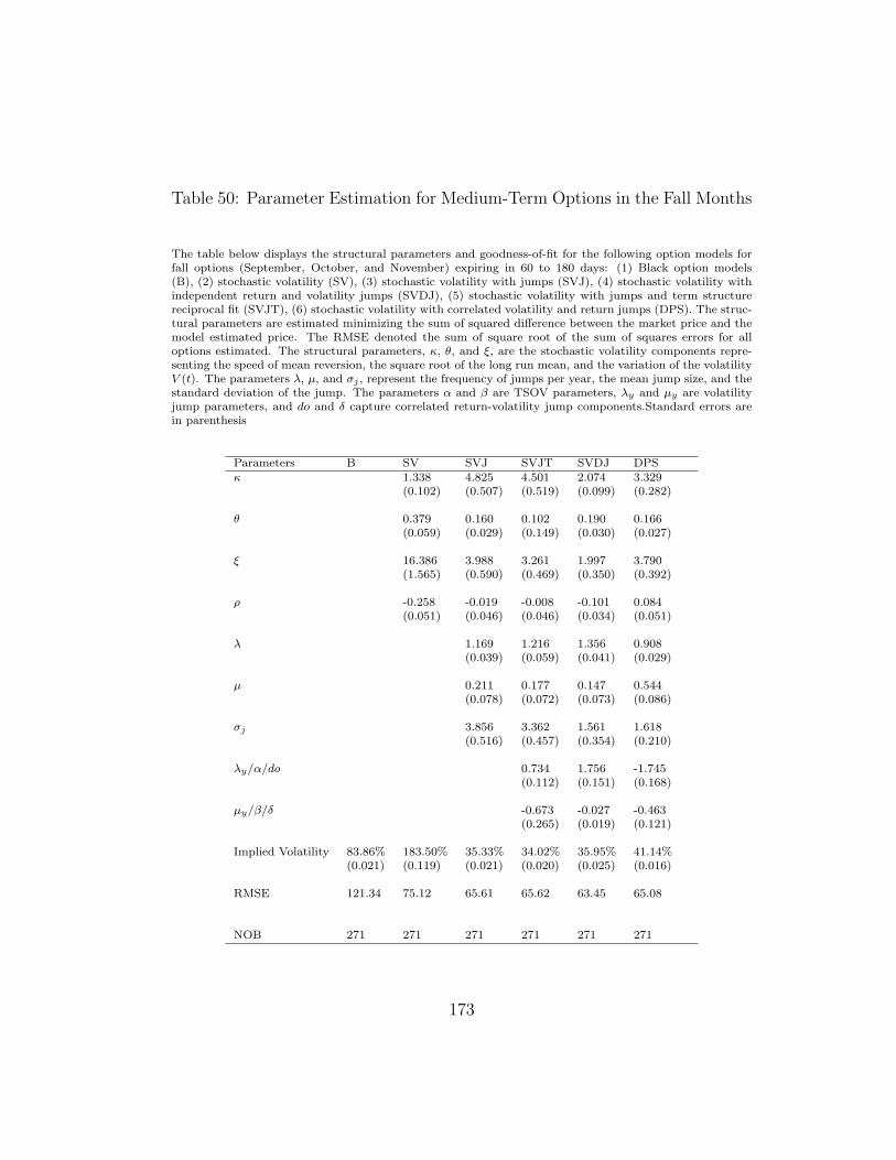
Table 50: Parameter Estimation for Medium-Term Options in the Fall Months
The table below displays the structural parameters and goodness-of-fit for the following option models forfall options (September, October, and November) expiring in 60 to 180 days: (1) Black option models(B), (2) stochastic volatility (SV), (3) stochastic volatility with jumps (SVJ), (4) stochastic volatility withindependent return and volatility jumps (SVDJ), (5) stochastic volatility with jumps and term structurereciprocal fit (SVJT), (6) stochastic volatility with correlated volatility and return jumps (DPS). The struc-tural parameters are estimated minimizing the sum of squared difference between the market price and themodel estimated price. The RMSE denoted the sum of square root of the sum of squares errors for alloptions estimated. The structural parameters, κ, θ, and ξ, are the stochastic volatility components repre-senting the speed of mean reversion, the square root of the long run mean, and the variation of the volatilityV (t). The parameters λ, µ, and σj , represent the frequency of jumps per year, the mean jump size, and thestandard deviation of the jump. The parameters α and β are TSOV parameters, λy and µy are volatilityjump parameters, and do and δ capture correlated return-volatility jump components.Standard errors arein parenthesis
Parameters B SV SVJ SVJT SVDJ DPSκ 1.338 4.825 4.501 2.074 3.329
(0.102) (0.507) (0.519) (0.099) (0.282)
θ 0.379 0.160 0.102 0.190 0.166(0.059) (0.029) (0.149) (0.030) (0.027)
ξ 16.386 3.988 3.261 1.997 3.790(1.565) (0.590) (0.469) (0.350) (0.392)
ρ -0.258 -0.019 -0.008 -0.101 0.084(0.051) (0.046) (0.046) (0.034) (0.051)
λ 1.169 1.216 1.356 0.908(0.039) (0.059) (0.041) (0.029)
µ 0.211 0.177 0.147 0.544(0.078) (0.072) (0.073) (0.086)
σj 3.856 3.362 1.561 1.618(0.516) (0.457) (0.354) (0.210)
λy/α/do 0.734 1.756 -1.745(0.112) (0.151) (0.168)
µy/β/δ -0.673 -0.027 -0.463(0.265) (0.019) (0.121)
Implied Volatility 83.86% 183.50% 35.33% 34.02% 35.95% 41.14%(0.021) (0.119) (0.021) (0.020) (0.025) (0.016)
RMSE 121.34 75.12 65.61 65.62 63.45 65.08
NOB 271 271 271 271 271 271
173

Table 51: Parameter Estimation for Short-Term Options in the Fall Months
The table below displays the structural parameters and goodness-of-fit for the following option models forfall options (September, October, and November) expiring in 60 days or less: (1) Black option models(B), (2) stochastic volatility (SV), (3) stochastic volatility with jumps (SVJ), (4) stochastic volatility withindependent return and volatility jumps (SVDJ), (5) stochastic volatility with jumps and term structurereciprocal fit (SVJT), (6) stochastic volatility with correlated volatility and return jumps (DPS). The struc-tural parameters are estimated minimizing the sum of squared difference between the market price and themodel estimated price. The RMSE denoted the sum of square root of the sum of squares errors for alloptions estimated. The structural parameters, κ, θ, and ξ, are the stochastic volatility components repre-senting the speed of mean reversion, the square root of the long run mean, and the variation of the volatilityV (t). The parameters λ, µ, and σj , represent the frequency of jumps per year, the mean jump size, and thestandard deviation of the jump. The parameters α and β are TSOV parameters, λy and µy are volatilityjump parameters, and do and δ capture correlated return-volatility jump components.Standard errors arein parenthesis
Parameters B SV SVJ SVJT SVDJ DPSκ 2.318 2.522 2.229 2.395 2.136
(0.373) (0.189) (0.118) (0.162) (0.051)
θ 0.821 0.336 0.110 0.214 0.433(0.381) (0.060) (0.051) (0.095) (0.045)
ξ 52.628 30.635 32.214 28.733 9.884(2.450) (3.227) (3.366) (3.059) (1.772)
ρ 0.576 0.363 0.338 0.349 0.152(0.050) (0.058) (0.058) (0.053) (0.051)
λ 1.903 2.603 2.623 0.727(0.544) (0.964) (0.970) (0.106)
µ 3.863 3.944 3.338 0.199(1.060) (0.755) (0.731) (0.036)
σj 2.648 2.705 2.871 2.638(0.265) (0.300) (0.452) (0.153)
λy/α/do 0.950 1.097 -0.451(0.014) (0.056) (0.266)
µy/β/δ -0.517 0.507 -0.160(0.126) (0.162) (0.053)
Implied Volatility 243.52% 279.16% 169.48% 151.37% 158.94% 81.60%(0.109) (0.120) (0.148) (0.157) (0.142) (0.050)
RMSE 54.79 1.79 1.02 0.80 0.55 0.39
NOB 114 114 114 114 114 114
174

Table 52: Market Price(s) of Risk
The table below shows the estimates for the market price(s) of risk. λs is the market price of risk. λσ
is the market price of volatility risk. λj and λjv are the market price of return-jump intensity risk andmarket price of volatility-jump intensity risk respectively. (SV) is the stoachstic volatility model, (SVJ) isthe stochastic volatility with jumps and (SVDJ) stochastic volatility with independent return and volatilityjumps. T-Stats are in parentheses. σ̂ is the average spot volatility.
Model λs λσ λj λjv σ̂
SV -0.37 -17.96 76.76%(1.83) (27.35)
SVJ 0.08 -5.15 0.42 51.91%(0.81) (12.04) (41.97)
SVDJ -0.04 -4.92 0.27 0.49 52.65%(0.62) (12.47) (16.86) (19.87)
175

Appendices
176
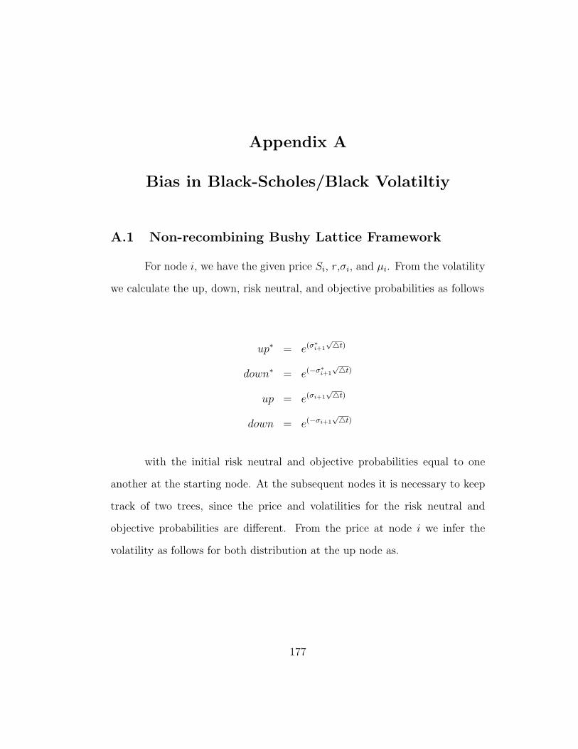
Appendix A
Bias in Black-Scholes/Black Volatiltiy
A.1 Non-recombining Bushy Lattice Framework
For node i, we have the given price Si, r,σi, and µi. From the volatility
we calculate the up, down, risk neutral, and objective probabilities as follows
up∗ = e(σ∗i+1
√4t)
down∗ = e(−σ∗i+1
√4t)
up = e(σi+1√4t)
down = e(−σi+1√4t)
with the initial risk neutral and objective probabilities equal to one
another at the starting node. At the subsequent nodes it is necessary to keep
track of two trees, since the price and volatilities for the risk neutral and
objective probabilities are different. From the price at node i we infer the
volatility as follows for both distribution at the up node as.
177

risk neutral:
dz∗2i =
S∗2i−S∗iS∗i
− r4tσ∗i
σ∗22i = σ∗2i + κ(θ − σ∗2i ) ∗ 4t− ξσ∗2i ∗ dz∗2i
S∗2(i+1) = up ∗ S∗i+1
objective:
dz2i =S2i−Si
Si− µ2i4tσi
σ22i = σ2
i + (κ(θ − σ2i ) + ξλσ2
i )4t− ξσ2i dz2i
µ2(i+1) = r + λσi+1
S2(i+1) = up ∗ Si+1
For the bottom node we have risk neutral:
dz∗2i =
S∗2i+1−S∗iS∗i
− r4tσ∗i
σ∗22i+1 = σ∗2i + κ(θ − σ∗2i ) ∗ 4t− ξσ∗2i ∗ dz∗2i
S∗2(i+1)+1 = down ∗ S∗i+1
objective:
dz2i =
S2i+1−Si
Si− µ2i4tσi
σ22i+1 = σ2
i + (κ(θ − σ2i ) + ξλσ2
i )4t− ξσ2i dz2i
µ2(i+1)+1 = r + λσi+1
S2(i+1)+1 = down ∗ Si+1
178
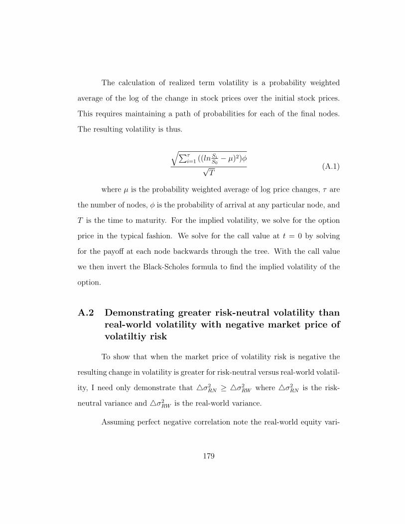
The calculation of realized term volatility is a probability weighted
average of the log of the change in stock prices over the initial stock prices.
This requires maintaining a path of probabilities for each of the final nodes.
The resulting volatility is thus.
√∑τi=1 ((ln Si
S0− µ)2)φ
√T
(A.1)
where µ is the probability weighted average of log price changes, τ are
the number of nodes, φ is the probability of arrival at any particular node, and
T is the time to maturity. For the implied volatility, we solve for the option
price in the typical fashion. We solve for the call value at t = 0 by solving
for the payoff at each node backwards through the tree. With the call value
we then invert the Black-Scholes formula to find the implied volatility of the
option.
A.2 Demonstrating greater risk-neutral volatility thanreal-world volatility with negative market price ofvolatiltiy risk
To show that when the market price of volatility risk is negative the
resulting change in volatility is greater for risk-neutral versus real-world volatil-
ity, I need only demonstrate that 4σ2RN ≥ 4σ2
RW where 4σ2RN is the risk-
neutral variance and 4σ2RW is the real-world variance.
Assuming perfect negative correlation note the real-world equity vari-
179

ance below:
4σ2RW = [κ(θ − σ2) + λξσ2]4t+ ξσ[
µ4t− 4SS
σ]
4σ2RW = [κ(θ − σ2) + λξσ2]4t+ ξσ[
(r + λσ)4t− 4SS
σ]
4σ2RW = [C + λξσA]4t+B
where
A = (σ + 1)
B = ξ(r − 4SS
)
C = κ(θ − σ2)
Now assume that θ = σ2 such that C = 0, a negative λ results in A
dampining the effect of B, thus muting 4σ2RW . For the risk-neutral process,
A = 0, and B fully impacts4σ2RN .On average through time it must be the case
that C = 0 given the mean-reverting nature of volatiltiy. Thus4σ2RN ≥ 4σ2
RW
180
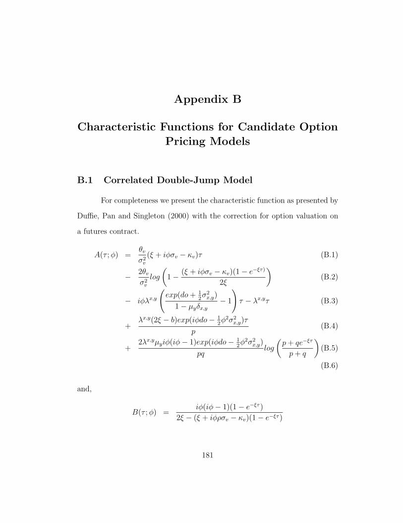
Appendix B
Characteristic Functions for Candidate Option
Pricing Models
B.1 Correlated Double-Jump Model
For completeness we present the characteristic function as presented by
Duffie, Pan and Singleton (2000) with the correction for option valuation on
a futures contract.
A(τ ;φ) =θv
σ2v
(ξ + iφσv − κv)τ (B.1)
− 2θv
σ2v
log
(1− (ξ + iφσv − κv)(1− e−ξτ)
2ξ
)(B.2)
− iφλx,y
(exp(do+ 1
2σ2
x,y)
1− µyδx,y
− 1
)τ − λx,yτ (B.3)
+λx,y(2ξ − b)exp(iφdo− 1
2φ2σ2
x,y)τ
p(B.4)
+2λx,yµyiφ(iφ− 1)exp(iφdo− 1
2φ2σ2
x,y)
pqlog
(p+ qe−ξτ
p+ q
)(B.5)
(B.6)
and,
B(τ ;φ) =iφ(iφ− 1)(1− e−ξτ )
2ξ − (ξ + iφρσv − κv)(1− e−ξτ )
181
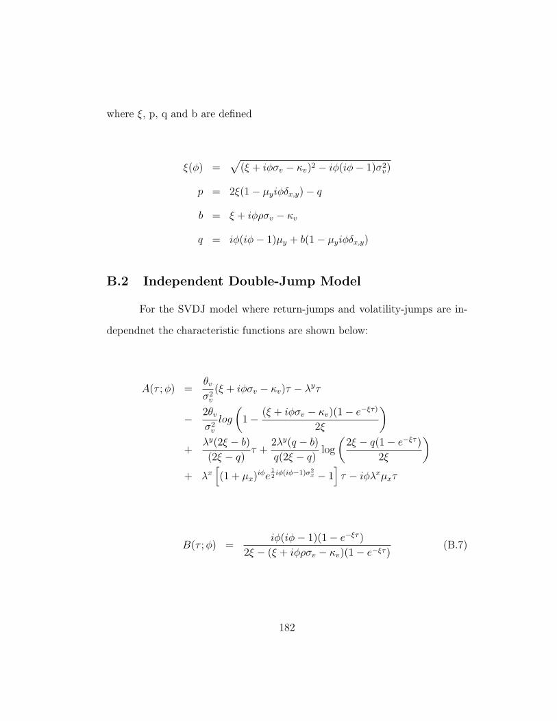
where ξ, p, q and b are defined
ξ(φ) =√
(ξ + iφσv − κv)2 − iφ(iφ− 1)σ2v)
p = 2ξ(1− µyiφδx,y)− q
b = ξ + iφρσv − κv
q = iφ(iφ− 1)µy + b(1− µyiφδx,y)
B.2 Independent Double-Jump Model
For the SVDJ model where return-jumps and volatility-jumps are in-
dependnet the characteristic functions are shown below:
A(τ ;φ) =θv
σ2v
(ξ + iφσv − κv)τ − λyτ
− 2θv
σ2v
log
(1− (ξ + iφσv − κv)(1− e−ξτ)
2ξ
)+
λy(2ξ − b)
(2ξ − q)τ +
2λy(q − b)
q(2ξ − q)log
(2ξ − q(1− e−ξτ )
2ξ
)+ λx
[(1 + µx)
iφe12iφ(iφ−1)σ2
x − 1]τ − iφλxµxτ
B(τ ;φ) =iφ(iφ− 1)(1− e−ξτ )
2ξ − (ξ + iφρσv − κv)(1− e−ξτ )(B.7)
182
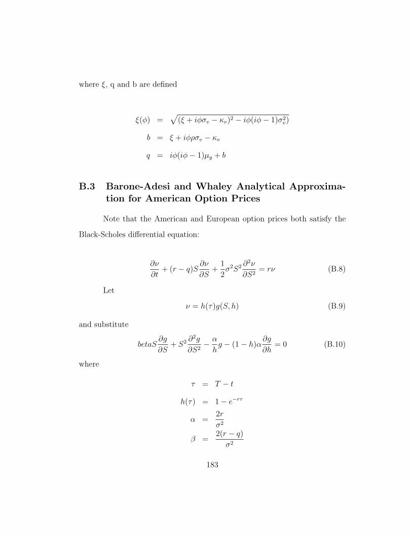
where ξ, q and b are defined
ξ(φ) =√
(ξ + iφσv − κv)2 − iφ(iφ− 1)σ2v)
b = ξ + iφρσv − κv
q = iφ(iφ− 1)µy + b
B.3 Barone-Adesi and Whaley Analytical Approxima-tion for American Option Prices
Note that the American and European option prices both satisfy the
Black-Scholes differential equation:
∂ν
∂t+ (r − q)S
∂ν
∂S+
1
2σ2S2 ∂
2ν
∂S2= rν (B.8)
Let
ν = h(τ)g(S, h) (B.9)
and substitute
betaS∂g
∂S+ S2 ∂
2g
∂S2− α
hg − (1− h)α
∂g
∂h= 0 (B.10)
where
τ = T − t
h(τ) = 1− e−rτ
α =2r
σ2
β =2(r − q)
σ2
183

The final term on the left-hand side is close to zero and can be ignored.
When τ is large, 1− h is close to zero; when τ is small, ∂g∂h
is close to zero.
Let the American call and put price at time τ be equal to C(S, t) and
P (S, t), where S is the stock price. Let c(S, t) and p(S, t) be equal to the
European call and put prices. Equation B.10 can be solved using standard
techniques. After boundary conditions have been found, the American Call is
equal to
C(S, t) =
{c(S, t) + A2(
SS∗
)γ2 , S < S∗
S −X, S ≥ S∗(B.11)
where S∗ is the critical price of the stock above which the option should
be exercised. It is estimated by solving
S∗ −X = c(S∗, t) +[1− e−q(T−t)N [d1(S∗)]
] S∗γ2
(B.12)
iteratively. For the put option, the valuation formula is
P (S, t) =
{p(S, t) + A2(
SS∗∗
)γ1 , S > S∗
X − S, S ≤ S∗(B.13)
where S∗∗ is the critical price of the stock below which the option should
be exercised. It is estimated by solving iteratively
X − S∗∗ = p(S∗∗, t) +[1− e−q(T−t)N [−d1(S∗∗)]
] S∗∗γ2
(B.14)
184

where
γ1 =
[−(β − 1)−
√(B − 1)2 + 4α
h
]2
γ2 =
[−(β − 1) +
√(B − 1)2 + 4α
h
]2
A1 = −(S∗∗
γ1
)(1− e−q(T−t)N [−d1(S∗∗)]
)A2 = −
(S∗
γ2
)(1− e−q(T−t)N [−d1(S∗)]
)While this formulation is for stock options, this quadratic approach can
easily be applied to options on futures contracts as the options are analogous
to stock options.
185
Index
Abstract, vi
Acknowledgments, v
Appendices, 176
Appendix
Bias in Black-Scholes/Black Volatiltiy,
177
Bibliography, 195
Bibliography, 187
Black implied volatility, 33
Black-Scholes, 1
Characteristic Functions for Candi-
date Option Pricing Models,
181
commands
environments
figure, 114–124
table, 125–129, 132, 134, 136,
137, 176
Dedication, iv
double-jump option model, 80
Empirical Performance of Option Mod-
els for Natural Gas and Es-
timation of the Market Price(s)
of Risk, 74
Estimating the bias, 22
Estimation of λσ, 66
Estimation of the Bias in BSIV/BIV,
19
Estimation Using Mean Reverting
Framework, 65
Evidence on the Market Price of Volatil-
ity Risk, 9
Independent Double Jumps and TSOV
considerations, 85
Introduction, 1
Mean-Reversion in Stochastic Volatil-
ity, 103
Modeling Issues, 80
Monte Carlo Simulation, 37
Monte Carlo Simulation and Esti-
mation of the Market Price
of Volatility Risk, 36
Out of sample pricing performance,
101
Parameter Estimation, including Mar-
ket Price of Risk, 106
Simulation within a Simulation, 61
Stochastic Volatility, 14
Structural Parameter Estimation and
Model Performance, 94
Tables and Figures, 113
The Bias in Black-Scholes/Black Im-
plied Volatility, 14
TSOV, 26
Understanding the volatility in gas
markets, 89
186
Bibliography
1. Ait-Sahalia, Y., and A. Lo, 1998, Nonparametric estimation of state-
price densities implicit in financial prices, Journal of Finance 53, No. 2,
499-548.
2. Anderson, T., Bollerslev, T., 1998. Answering the Skeptics: Yes, Stan-
dard Volatility Models do provide Accurate Forecasts. International Eco-
nomic Review 39, 885-905
3. Andersen, T., T. Bollerslev, F. Diebold, and H. Ebens, 2001. The dis-
tribution of stock return volatility. Journal of Financial Economics 61.
4. Andersen, T., L. Benzoni, J. Lund, 2002, An empirical investigation of
continuous-time equity return models, Journal of Finance 57, 1239-1284.
5. Bakshi, G., and C. Cao, 2003, Risk-Neutral Kurtosis, Jumps, and Option
Pricing: Evidence from 100 Most Actively Traded Firms on the CBOE,
Working Paper, University of Maryland
6. Bakshi, G., Cao, C., Chen, Z., 1997. Empirical performance of alterna-
tive option pricing models. Journal of Finance 52, 2003-2049.
7. Bakshi, G., C. Cao, and Z. Chen, 2000, Pricing and hedging long-term
options, Journal of Econometrics 94, 277-318.
187
8. Bakshi, G., Kapadia, N., 2001. Delta-hedged gains and the pricing of
volatility risk. Working paper, University of Massachusetts, Amherst.
9. Bakshi, G., N. Kapadia, D. Madan, 2003, Stock return characteristics,
skew laws, and the differential pricing of individual equity options, Re-
view of Financial Studies 16 (1), 101-143.
10. Ball, C., and W. Torous, 1985, On jumps in common stock prices and
their impact on call option pricing, Journal of Finance 40, 155-173.
11. Barone-Adesi, G., and R. Whaley, 1987, Efficient analytic approximation
of American option values, Journal of Finance 42, 301-320.
12. Bates, D., 1996. Jumps and Stochastic Volatility: Exchange Rate Pro-
cesses Implicit in Deutsche Mark Options. Review of Financial Studies
9, 69-107.
13. Bates, D., 2000. Post 87’ crash fears in S&P 500 futures options. Journal
of Econometrics 94, 181-238
14. Benzoni, L. (1998). Pricing options under stochastic volatility: An
econometric analysis. Working paper, Kellogg Graduate School of Man-
agement, Northwestern University.
15. Black, F., and M. Scholes, 1973, The pricing of options and corporate
liabilities, Journal of Political Economy 81, 637-659.
188
16. Black, F., 1976. Studies of stock price volatility changes. Proceedings
of the 1976 Meetings of the Business and Economics Statistics Section,
American Statistical Association, pp. 177-181.
17. Buraschi, A., and J. Jackwerth, 2001, ”The price of a smile: Hedging
and spanning in option markets,” Review of Financial Studies 14, No.2,
495-527
18. Canina, L. and S. Figlewski, 1993. The information content of Implied
Volatility. The Review of Financial Studies 6, 659-681.
19. Carr, P., H. Geman, D. Madan, and M. Yor, 2002, The fine structure of
asset returns: an empirical investigation, Journal of Business 75, Volume
2, 19-37.
20. Carr, P., and L. Wu, 2002, The finite moment log stable process and
option pricing, Journal of Finance (forthcoming).
21. Chernov, M. and E. Ghysels (2000). A study towards a unified approach
to the joint estimation of objective and risk neutral measures for the
purpose of options valuation. Journal of Financial Economics 56, 407-
458.
22. Christensen, B and N. Prabhala, 1998, ”The relationship between im-
plied and realized volatility,” Journal of Financial Economics 50, 125-150
23. Christoffersen, P and K. Jacobs, 2001, ”The Importance of the Loss
Function in Option Pricing,” McGill Working Paper
189
24. Coval, J., and T.Shumway, 2000, ”Expected Option Returns,” Journal
of Finance (forthcoming)
25. Cox, J. C., J. E. Ingersoll, and S. A. Ross, 1985. A theory of the term
structure of interest rates. Econometrica 53 (2), 385-407.
26. Das, S., 2002, The surprise element: jumps in interest rates, Journal of
Econometrics 106, 27-65.
27. Dennis, P., and S. Mayhew, 2002, Implied volatility skews: evidence from
options on individual securities, Journal of Financial and Quantitative
Analysis 37, No. 3, 471-493.
28. Dincerler, C., Ronn, E., 2001. Risk Premia and Price Dynamics in
Electric Power Markets. University of Texas working paper.
29. Duffie, D., J. Pan, and K. Singleton, 2000, Transform analysis and asset
pricing for affine jump-diffusions, Econometrica 68, 1343-1376.
30. Duffie, D. and K. Singleton, 1993, Simulated moments estimation of
markov models of asset prices, Econometrica 61, 929-952.
31. Dumas, B., J. Fleming, R. Whaley, 1998, Implied volatility functions:
empirical tests, Journal of Finance, 53 (6), 2059-2106.
32. Eberlein, E., U. Keller, K. Prause, 1998, New insights into smile, mis-
pricing, and value at risk: the hyperbolic model, Journal of Business 71,
No. 2, 371-405.
190
33. Eichenbaum, M., L. Hansen, K. Singleton, 1988, A time series analysis
of representative agent models of consumption and leisure choice under
uncertainty, Quarterly Journal of Economics, No. 1 (February), 51-78.
34. Eraker, B., 2001. Do stock prices and volatility jump? reconciling evi-
dence from spot and option prices. Working paper, Graduate School of
Business, University of Chicago
35. Eraker, B., M. Johannes, N. Polson, 2002, The impact of jumps in volatil-
ity and returns, Journal of Finance (forthcoming).
36. Fama, E., and J. McBeth, 1973, Risk, return, and equilibrium: empirical
tests, Journal of Political Economy 81, 607-636.
37. Gallant, A. R. and G. Tauchen, 1998. Reprojecting partially observed
systems with application to interest rate diffusions. Journal of American
Statistical Association 93,10-24.
38. Hansen, L., 1982, Large sample properties of generalized method of mo-
ments estimators, Econometrica 50, 1029-1084.
39. Hansen, B., 1992, The likelihood ratio test under nonstandard condi-
tions: testing the Markov switching model of GNP, Journal of Applied
Econometrics 7, S61-S82.
40. Heston, S., 1993. A closed-form solution of options with stochastic
volatility with applications to bond and currency options. The Review
of Financial Studies 6, 327-343.
191

41. Heston, S., and S. Nandi, 2000, A closed-form GARCH option valuation
model, Review of Financial Studies 13, 585-625.
42. Hentschel, L., 2002. Errors in Implied Volatility Estimation. Forthcom-
ing in the Journal of Financial and Quantitative Analysis
43. Huang, J., and L. Wu, 2002, Specification analysis of option pricing mod-
els based on time-changed Levy processes, mimeo, Fordham University.
44. Hull, J., White, A., 1987. The pricing of options on assets with stochastic
volatilities. Journal of Finance 42, 281-300.
45. Jackwerth, J. C. and M. Rubinstein, 1996. Recovering probability dis-
tributions from option prices. Journal of Finance 51, 1611-1631.
46. Jorion, P., 1995. Predicting volatility in the foreign exchange markets.
Journal of Finance 6, 327-343.
47. Jones, C., 2001. The Dynamics of Stochastic Volatility: Evidence from
the underlying and options markets. Unpublished paper, Simon School,
University of Rochester, Rochester, NY.
48. Kendall, M., and A. Stuart, 1977, The Advanced Theory of Statistics,
Volume 1, McMillan Publishing Co. New York.
49. Lamoureux, C.G., Lastrapes, W., 1993. Forecasting stock return vari-
ance: towards understanding stochastic implied volatility. Review of
Financial Studies 6, 293-326.
192
50. Longstaff, F., 1995, Option pricing and the martingale restriction, Re-
view of Financial Studies 8, No. 4, 1091-1124.
51. Madan, D., P. Carr, and E. Chang, 1998, The variance gamma process
and option pricing, European Journal of Finance 1, 39-55.
52. Merton, R., 1976, Option pricing when underlying stock returns are
discontinuous, Journal of Financial Economics 3, 125-144.
53. Newey, W., and K. West, 1987, A simple positive semi-definite het-
eroskedasticity and autocorrelation consistent covariance matrix, Econo-
metrica 55 (4), 703-708.
54. Pan, J., 2000. Jump-Diffusion Models of Asset Prices: Theory and Em-
pirical Evidence. Ph. D. Thesis, Graduate School of Business, Stanford
University.
55. Pan, J., 2002, The jump-risk premia implicit in options: evidence from
an integrated time-series study, Journal of Financial Economics 63, No.
1, 3-50.
56. Rubinstein, M., 1985, Nonparametric tests of alternative option pricing
models using all reported trades and quotes on the 30 most active CBOE
options classes from August 23, 1976 through August 31, 1978, Journal
of Finance 40, 455-480.
57. Rubinstein, M., 1994. Implied binomial trees. Journal of Finance 49,
771-818.
193
58. Singleton, K., 2001, Estimation of affine asset pricing models using the
empirical characteristic function, Journal of Econometrics, Vol. 102,
111-141.
59. Stanton, R., 1997. A Nonparametric Model of Term Structure Dynamics
and the Market Price of Interest Rate Risk. Journal of Finance 52, 1973-
2002.
60. Schwartz, E., 1997. The Stochastic Behavior of Commodity Prices: Im-
plications for Valuation and Hedging. Journal of Finance 52, 923-973.
61. Stein, J., 1989. Overreaction in the options market. Journal of Finance
44, 1011-1023.
62. Whaley, R., 1982, Valuation of American calls on dividend-paying stocks,
Journal of Financial Economics 10, 29-58.
194
Vita
James Stephen Doran was born in London, England on 27 August 1975,
the son of Charles J. Doran and Elaine M. Doran. He received the Bachelor of
Arts degree in Economics from Emory University in 1997. At Emory, he was
recognized as 2nd-team Academic All-America in Soccer in 1997. Subsequent
to graduation, he applied to the University of Texas at Austin for enrollment
in their finance program. He was accepted and started graduate studies in
August, 1998. Starting in August 2004, he will begin as Assistant Professor
at Florida State University.
Permanent address: 2000 Cullen Ave #15Austin, Texas 78757
This dissertation was typeset with LATEX† by the author.
†LATEX is a document preparation system developed by Leslie Lamport as a specialversion of Donald Knuth’s TEX Program.
195