Coronavirus Optimization Algorithm: A bioinspired

metaheuristic based on the COVID-19 propagation

model

F. Martınez-Alvarez1∗, G. Asencio-Cortes1, J. F. Torres1,

D. Gutierrez-Aviles1, L. Melgar-Garcıa1, R. Perez-Chacon1,

C. Rubio-Escudero2, J. C. Riquelme2, A. Troncoso1

1Data Science & Big Data Lab, Pablo de Olavide University, ES-41013

Seville, Spain

2Department of Computer Science, University of Seville, ES-41012

Seville, Spain

Abstract

A novel bioinspired metaheuristic is proposed in this work, simulating how the

coronavirus spreads and infects healthy people. From an initial individual (the

patient zero), the coronavirus infects new patients at known rates, creating new

populations of infected people. Every individual can either die or infect and, af-

terwards, be sent to the recovered population. Relevant terms such as re-infection

probability, super-spreading rate or traveling rate are introduced in the model in or-

der to simulate as accurately as possible the coronavirus activity. The Coronavirus

Optimization Algorithm has two major advantages compared to other similar strate-

gies. First, the input parameters are already set according to the disease statistics,

∗Corresponding author, fmaralv@upo.es

1

arX

iv:2

003.

1363

3v2

[cs

.AI]

16

Apr

202

0

preventing researchers from initializing them with arbitrary values. Second, the ap-

proach has the ability of ending after several iterations, without setting this value

either. Infected population initially grows at an exponential rate but after some

iterations, when considering social isolation measures and the high number recov-

ered and dead people, the number of infected people starts decreasing in subsequent

iterations. Furthermore, a parallel multi-virus version is proposed in which several

coronavirus strains evolve over time and explore wider search space areas in less it-

erations. Finally, the metaheuristic has been combined with deep learning models,

in order to find optimal hyperparameters during the training phase. As applica-

tion case, the problem of electricity load time series forecasting has been addressed,

showing quite remarkable performance.

Keywords: Metaheuristics, soft computing, deep learning, Coronavirus.

1 Introduction

The coronavirus (COVID-19) is a new respiratory virus, firstly discovered in humans in

December 2019, that has spread worldwide, having been reported more than 1 million

infected people so far. Much remains unknown about the virus, including how many

people may have very mild or asymptomatic infections, and whether they can transmit

the virus. The precise dimensions of the outbreak are hard to know.

Bioinspired models typically mimic behaviors from the nature and are known for

their successful application in hybrid approaches to find parameters in machine learning

model optimization. Viruses can infect people and these people can either die, infect

other people or simply get recovered after the disease. Vaccines and the immune defense

system typically fight the disease and help to mitigate their effects while an individual is

still infected. This behavior is typically modeled by an SIR model, consisting of three

kind of individuals: S for the number of susceptible, I for the number of infectious, and

R for the number of recovered.

Metaheuristics must deal with huge search spaces, even infinite for the continuous

cases, and must find suboptimal solutions in reasonable execution times. The rapid prop-

2

agation of the coronavirus along with its ability of infecting most of the countries in the

world impressively fast, has inspired the novel metaheuristic proposed in this work, named

Coronavirus Optimization Algorithm (CVOA). A parallel version is also proposed in order

to spread different coronavirus strains and achieve better results in less iterations.

The main CVOA advantages regarding other similar approaches can be summarized

as follows:

1. Coronavirus statistics are known by the scientific community. In this sense, the rate

of infection, the mortality rate or the re-infection probability are already known.

That is, CVOA is parametrized with actual values for rates and probabilities, pre-

venting the user to perform an additional study on the most suitable setup config-

uration.

2. CVOA can stop the solutions exploration after several iterations, with no need to

be configured. That is, the number of infected people increases during the first

iterations, however, after a certain number of iterations, the number of infected

people starts decreasing, until reaching a void infected set of individuals.

3. The coronavirus high spreading rate is useful for exploring promising regions more

thoroughly (intensification) while the use of parallel strains ensures that all regions

of the search space are evenly explored (diversification).

4. Another relevant contribution of this work is the proposal of a new codification,

discrete and of dynamic length, specifically designed for combining Long Short-

Term Memory networks (LSTM) with CVOA (or any other metaheuristic).

As for the limitations of the current approach, there is mainly one. Since there is

no vaccine currently, it has not been included in the procedure to reduce the number

of individuals candidates to be infected. This fact involves an exponential increase of

the infected population in the first iterations and, therefore, an exponential increase of

the execution time for such iterations. This fact, however, is partially solved with the

social isolation measures that simulate individuals that cannot be infected at a particular

iteration.

3

A study case is included in this work to discuss the CVOA performance. CVOA has

been used to find the optimal values for the hyperparameters of a LSTM architecture [17],

which is widely used model for artificial recurrent neural network (RNN), in the field of

deep learning [8]. Data from the Spanish electricity consumption have been used to vali-

date the accuracy. The results achieved verge on 0.45%, substantially outperforming other

well-established methods such as random forest, gradient-boost trees, linear regression or

deep learning optimized with other metaheuristics. The code, developed in Phyton with a

discrete codification, is available in the supplementary material (along with an academic

version in Java for a binary codification).

Finally, it is acknowledged the need of further study on the performance of well-

known functions [16], however, given the relevance of coronavirus is acquiring throughout

the world (declared as pandemic by the World Health Organization) and the remarkable

results achieved when combined with deep learning, it was wanted to share this work

hoping it inspires future research in this direction.

The rest of the paper is organized as follows. Section 2 discusses related and recent

works. The methodology proposed is introduced in Section 3. Section 4 proposes a

discrete codification to hybridize deep learning models with CVOA and provides some

illustrative cases. A preliminary analysis on how populations are created and evolved

over time is discussed in Section 5. The results achieved are reported and discussed in

Section 6. Finally, the conclusions drawn and future work suggestions are included in

Section 7.

2 Related works

There are many bioinspired metaheuristics to solve optimization problems. Although

CVOA has been conceived to optimize any kind of problems, this section focuses on

optimization algorithms applied to hybridize deep learning models.

It is hard to find consensus among the researchers on which method should be applied

to which problem, and, for this reason, many optimization methods have been proposed

during the last decade to improve deep learning models. Generally, the criterion for

4

selecting a method is its associated performance from a wide variety of perspectives. Low

computation cost, accuracy or even implementation difficulty can be accepted as one of

these criteria.

The Virus Optimization Algorithm (VOA) was proposed by Liang and Cuevas-Juarez

in 2016 [18] and later improved in [19]. However, as many other metaheuristics, the

results of its application are highly dependent on its initial configuration. Additionally, it

simulates generic viruses, without adding individualized properties for particular viruses.

The results achieved indicate that its usefulness is beyond doubt.

One of the most extended metaheuristics used to improve deep learning parameters is

genetic algorithms (GA). Hence, a LSTM network optimized with GA can be found in [6].

To evaluate the proposed hybrid approach, the daily Korea Stock Price Index data were

used, outperforming the benchmark model. In 2019, a network traffic prediction model

based on LSTM and GA was proposed in [5]. The results were compared to pure LSTM

and ARIMA, reporting higher accuracy.

Multi-agents systems have also been applied to optimize deep learning models. The

use of Particle Swarm Optimization (PSO) can be found in [20]. The authors proposed a

model based on kernel principal component analysis and back propagation neural network

with PSO for midterm power load forecasting. The hybridization of deep learning models

with PSO was also explored in [13] but, this time, the authors applied the methodology

with image classification purposes.

Ants colony optimization (ACO) models have also been used to hybridize deep learn-

ing. Thus, Desell et al. [9] proposed an evolving deep recurrent neural networks using

ACO applied to the challenging task of predicting general aviation flight data. The work

in [12] introduced a method based on ACO to optimize a LSTM recurrent neural net-

works. Again, the field of application was flight data records obtained from an airline

containing flights that suffered from excessive vibration.

Some papers exploring the Cuckoo Search (CS) properties have been published recently

as well. In [23], CS was used to find suitable heuristics for adjusting the hyper-parameters

of another LSTM network. The authors claimed an accuracy superior to 96% for all the

5

datasets examined. Nawi et al. [22] proposed the use of CS to improve the training of RNN

in order to achieve fast convergence and high accuracy. Results obtained outperformed

those than other metaheuristics.

The use of the artificial bee colony (ABC) optimization algorithm applied to LSTM

can also be found in the literature. Hence, and optimized LSTM with ABC to forecast

the bitcoin price was introduced in [26]. The combination of ABC and RNN was also

proposed in [3] for traffic volume forecasting. This time the results were compared to

standard backpropagation models.

From the analysis of these works, it can be concluded that there is an increasing

interest in using metaheuristics in LSTM models. However, not as many works as for

artificial neural networks can be found in the literature and, none of them, based on a

virus propagation model. These two facts, among others, justify the application of CVOA

to optimize LSTM models.

3 Methodology

This section introduces the CVOA methodology. Thus, Section 3.1 describes the steps for

a single strain. Section 3.2 introduces the modifications added to use CVOA as a parallel

version. Section 3.3 suggests how parameters must be set. Section 3.4 shows the CVOA

pseudo codes and comments them.

3.1 Steps

Step 1. Generation of the initial population. The initial population consists of one

individual, the so-called patient-zero (PZ). As in the coronavirus epidemic, it identifies

the first human being infected.

Step 2. Disease propagation. Depending on the individual, several cases are evaluated:

1. Some of the infected individuals die. They die according to the coronavirus death

rate (P DIE). Such individuals can no longer infect new individuals.

6

2. The individuals surviving the coronavirus will infect new individuals (intensifica-

tion). Two types of spreading are considered, according to a given probability

(P SUPERSPREADER):

• Ordinary spreaders. Infected individuals will infect new ones according to the

coronavirus spreading rate (SPREADING RATE).

• Super-spreaders. Infected individuals will infect new ones according to the

coronavirus superspreading rate (SUPERSPREADING RATE).

3. There is another consideration, since it is needed to ensure diversification. Both

ordinary and super-spreaders individuals can travel and explore solutions quite

dissimilar. Therefore, individuals have a probability of traveling (P TRAV EL)

thus allowing to propagate the disease to solutions that may be quite different

(TRAV ELER RATE). In case of not being traveler, new solutions will change

according to an ORDINARY RATE. Note that one individual can be both super-

spreader and traveler.

Step 3. Updating populations. Three populations are maintained and updated for each

generation.

1. Dead population. If any individual dies, it is added to this population and can never

be used again.

2. Recovered population. After each iteration, infected individuals (after spreading the

coronavirus according to the previous step) are sent to the recovered population.

It is known that there is a reinfection probability. Hence, an individual belong-

ing to this population could be re-infected at any iteration provided that it meets

the reinfection criterion (P REINFECTION). Another situation must be consid-

ered, since individuals can be isolated simulating they are implementing the social

distancing measures. For the sake of simplicity, it is considered that an isolated

individual is sent to the recovered population as well when meeting an isolation

probability (P ISOLATION).

7

3. New infected population. This population gathers all individuals infected at each

iteration, according the procedure described in the previous steps. It is possible that

repeated new infected individuals are created at each iteration and, consequently,

it is recommended to remove such repeated individuals from this population before

the next iteration starts running.

Step 4. Stop criterion. One of the most interesting features of the proposed approach

lies on its ability to end without the need of controlling any parameter. This situation

occurs because the recovered and dead populations are constantly growing as time goes

by, and the new infected population cannot infect new individuals. It is expected that

the number of infected individuals increases for a certain number of iterations. However,

from a particular iteration on, the size of the new infected population will be smaller than

that of the current one because recovered and dead populations are too big, and the size

of the infected population decays over time. Additionally, a preset number of iterations

(PANDEMIC DURATION) can be added to the stop criterion. The social isolation

measures also contributes to reaching the stop criterion.

3.2 Remarks for a parallel CVOA version

It must be noted that it is very simple to use CVOA in a multi-virus version since it can

be implemented as a population-based algorithm, when considering the pandemic as a

set of intelligent agents each of them evolving in parallel. In contrast to trajectory-based

metaheuristics, population-based focuses on the diversification in the search space.

For this case, a new variable must be defined, strains, which will determine the number

of strains that will be launched in parallel. Each strain could simulate different regions.

In other words, strains can be differently configured so that each of them intensifies with

their own rates.

Several considerations must be done for this case:

1. Every strain is run independently, following the steps in the previous section.

2. A wise strategy should be followed to generate PZs for each strain. For instance,

8

it is suggested the generation of orthogonal PZs or with high Hamming distances.

That way, a wider search space could be covered, enhancing diversification.

3. The interaction between the different strains is done by means of dead and recov-

ered populations, which must be shared by all the strains. Operations over these

populations must be handled as concurrent updates [11].

4. New infected populations, on the contrary, are different for each strain and no

concurrent operations are required.

5. This version may help to simulate different rates for different strains. That way, if

there is any initial information about the search space, some strains could be more

focused on diversification and some others on intensification.

Depending on the hardware resources and how busy they are, every strain may evolve

at different speeds. This situation should not pose any problems since it is known that

the pandemic evolves at different rates and starts at different time stamps depending on

region of the world.

Last, another application can be found for this parallel version. CVOA emulates an

SIR model and consequently, any other global pandemic could be modeled by using the

known rates of, for instance, the flu of 1918 or 1957, another coronavirus SARS or MERS,

HIV, or Ebola. Hypothetically, parallel pandemics could be run with different rates.

3.3 Suggested parameters setup

Since CVOA simulates the coronavirus disease propagation, most of the rates (propaga-

tion, re-infection or mortality) are already known. This fact prevents the research from

wasting time in selecting values for such rates and turns the CVOA into metaheuristic

quite easy to execute.

However, it must be noted that the current rates are not definitive yet and it is

expected they will vary over time, as the pandemic evolves. Maybe these values will not

be stable until 2021 or even 2022. The suggested values have been retrieved from the

World Health Organization [1] and are discussed below:

9

1. P DIE. An infected individual can die with a given probability. Currently, this

rate is set as almost 5% by the scientific community. Therefore, P DIE = 0.05.

2. P SUPERSPREADER. It is the probability that an individual spread the disease

to a greater number of healthy individuals. It is known that this situation affects

to a 10% of the population, therefore, P SUPERSPREADER = 0.1. After this

condition is validated, two situations can be found:

• ORDINARY RATE. If the infected individual is not a super-spreader, then

the infection rate (also known as reproductive number, R0) is 2.5. It is sug-

gested that this rate varies from 0 to 5.

• SUPERSPREADER RATE. If the infected individual turns out to be

super-spreader, then he/she infects up to 15 healthy individuals on average. It

is suggested that this rate varies from 6 to 15.

3. P REINFECTION . It is known that a recovered individual can be re-infected.

The current reported rate is 14%. Therefore, P REINFECTION = 0.14.

4. P ISOLATION . This value is uncertain because countries are taking different

measures for social isolation. This parameter helps to reduce the exponential growth

of the infected population after each iteration. Therefore, a high value must be

assigned to this probability. It is suggested that P ISOLATION = 0.5.

5. P TRAV EL. This probability simulates how an infected individual can travel to

any place in the world and can infect healthy individuals. It is known that almost

a 10% of the population travel during a week (simulated time for every iteration),

so P TRAV EL = 0.1.

6. PANDEMIC DURATION . This parameter simulates the duration of the pan-

demic. Since the estimated recovering time is one week, each iteration simulates

one week. Currently, this data is unknown so this number can be adjusted to the

size of the problem. It is suggested that PANDEMIC DURATION = 30.

10

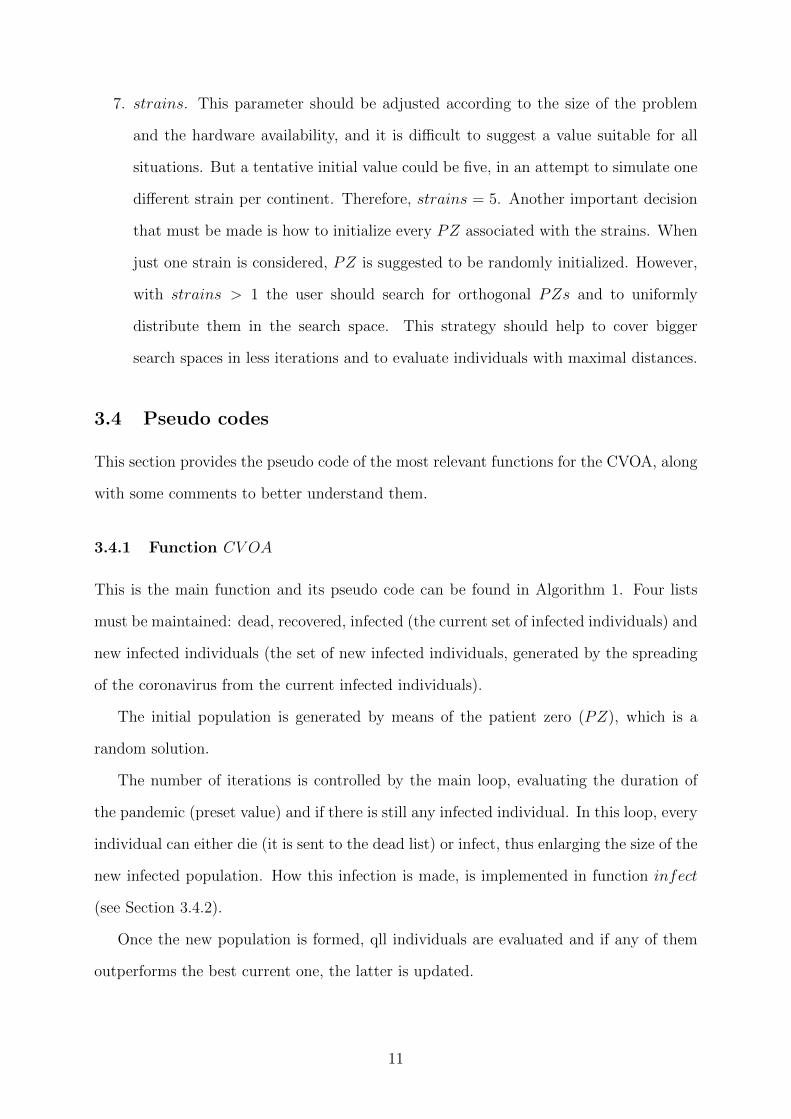
7. strains. This parameter should be adjusted according to the size of the problem

and the hardware availability, and it is difficult to suggest a value suitable for all

situations. But a tentative initial value could be five, in an attempt to simulate one

different strain per continent. Therefore, strains = 5. Another important decision

that must be made is how to initialize every PZ associated with the strains. When

just one strain is considered, PZ is suggested to be randomly initialized. However,

with strains > 1 the user should search for orthogonal PZs and to uniformly

distribute them in the search space. This strategy should help to cover bigger

search spaces in less iterations and to evaluate individuals with maximal distances.

3.4 Pseudo codes

This section provides the pseudo code of the most relevant functions for the CVOA, along

with some comments to better understand them.

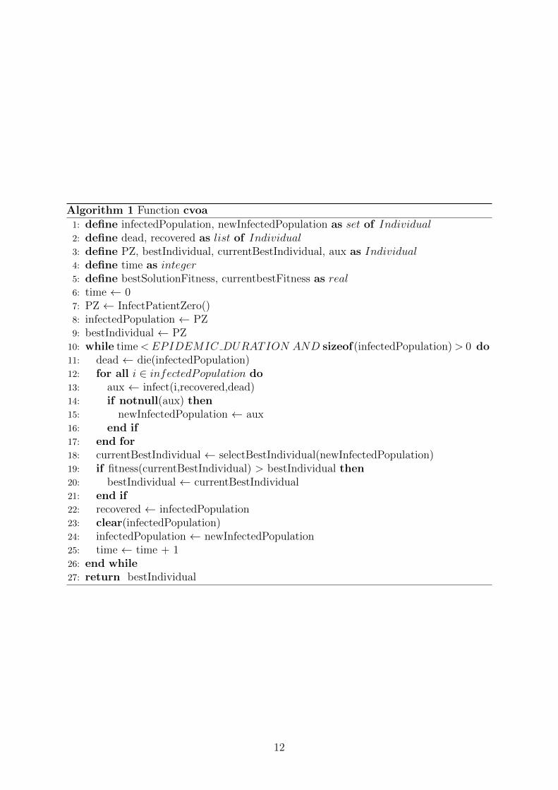
3.4.1 Function CV OA

This is the main function and its pseudo code can be found in Algorithm 1. Four lists

must be maintained: dead, recovered, infected (the current set of infected individuals) and

new infected individuals (the set of new infected individuals, generated by the spreading

of the coronavirus from the current infected individuals).

The initial population is generated by means of the patient zero (PZ), which is a

random solution.

The number of iterations is controlled by the main loop, evaluating the duration of

the pandemic (preset value) and if there is still any infected individual. In this loop, every

individual can either die (it is sent to the dead list) or infect, thus enlarging the size of the

new infected population. How this infection is made, is implemented in function infect

(see Section 3.4.2).

Once the new population is formed, qll individuals are evaluated and if any of them

outperforms the best current one, the latter is updated.

11

Algorithm 1 Function cvoa

1: define infectedPopulation, newInfectedPopulation as set of Individual2: define dead, recovered as list of Individual3: define PZ, bestIndividual, currentBestIndividual, aux as Individual4: define time as integer5: define bestSolutionFitness, currentbestFitness as real6: time ← 07: PZ ← InfectPatientZero()8: infectedPopulation ← PZ9: bestIndividual ← PZ

10: while time < EPIDEMIC DURATION AND sizeof(infectedPopulation) > 0 do11: dead ← die(infectedPopulation)12: for all i ∈ infectedPopulation do13: aux ← infect(i,recovered,dead)14: if notnull(aux) then15: newInfectedPopulation ← aux16: end if17: end for18: currentBestIndividual ← selectBestIndividual(newInfectedPopulation)19: if fitness(currentBestIndividual) > bestIndividual then20: bestIndividual ← currentBestIndividual21: end if22: recovered ← infectedPopulation23: clear(infectedPopulation)24: infectedPopulation ← newInfectedPopulation25: time ← time + 126: end while27: return bestIndividual

12

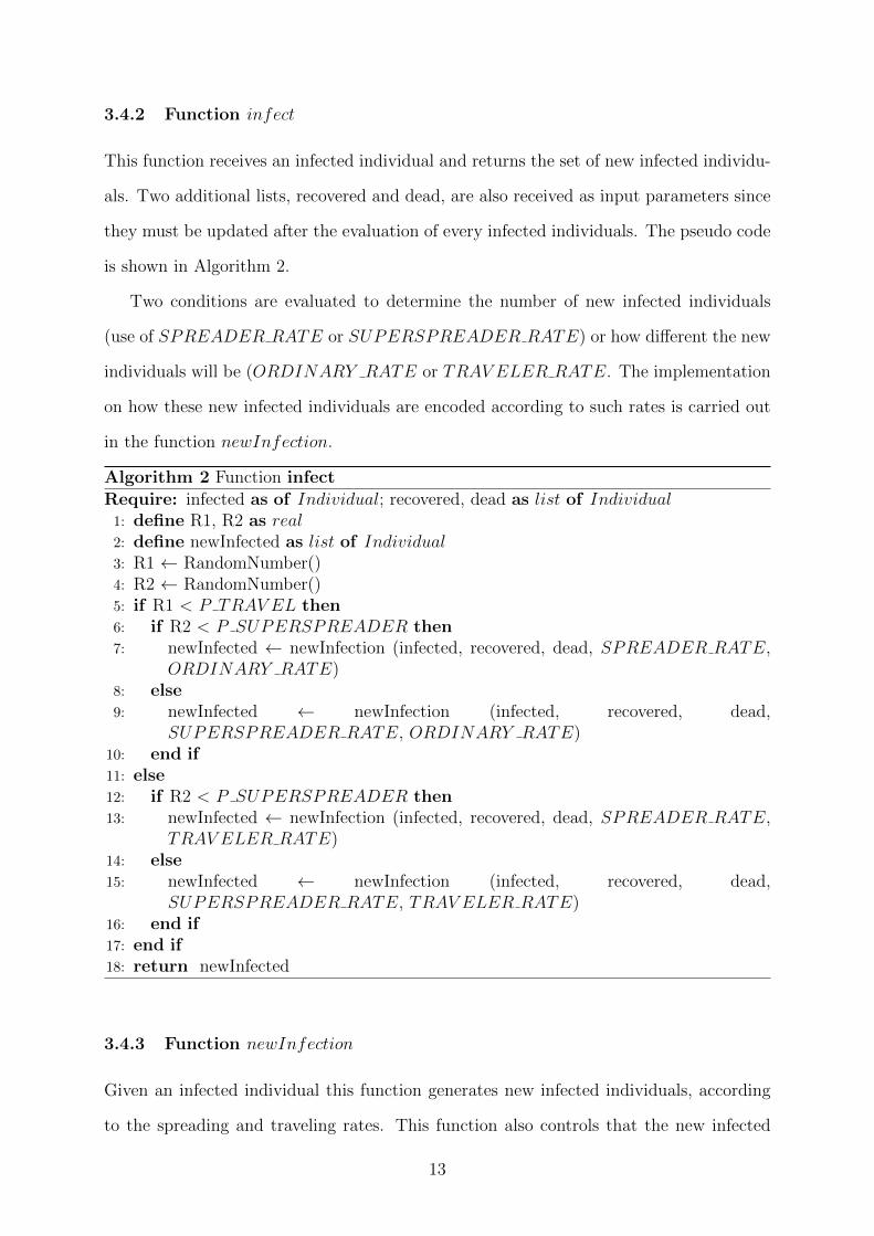
3.4.2 Function infect

This function receives an infected individual and returns the set of new infected individu-

als. Two additional lists, recovered and dead, are also received as input parameters since

they must be updated after the evaluation of every infected individuals. The pseudo code

is shown in Algorithm 2.

Two conditions are evaluated to determine the number of new infected individuals

(use of SPREADER RATE or SUPERSPREADER RATE) or how different the new

individuals will be (ORDINARY RATE or TRAV ELER RATE. The implementation

on how these new infected individuals are encoded according to such rates is carried out

in the function newInfection.

Algorithm 2 Function infect

Require: infected as of Individual; recovered, dead as list of Individual1: define R1, R2 as real2: define newInfected as list of Individual3: R1 ← RandomNumber()4: R2 ← RandomNumber()5: if R1 < P TRAV EL then6: if R2 < P SUPERSPREADER then7: newInfected ← newInfection (infected, recovered, dead, SPREADER RATE,

ORDINARY RATE)8: else9: newInfected ← newInfection (infected, recovered, dead,

SUPERSPREADER RATE, ORDINARY RATE)10: end if11: else12: if R2 < P SUPERSPREADER then13: newInfected ← newInfection (infected, recovered, dead, SPREADER RATE,

TRAV ELER RATE)14: else15: newInfected ← newInfection (infected, recovered, dead,

SUPERSPREADER RATE, TRAV ELER RATE)16: end if17: end if18: return newInfected

3.4.3 Function newInfection

Given an infected individual this function generates new infected individuals, according

to the spreading and traveling rates. This function also controls that the new infected

13

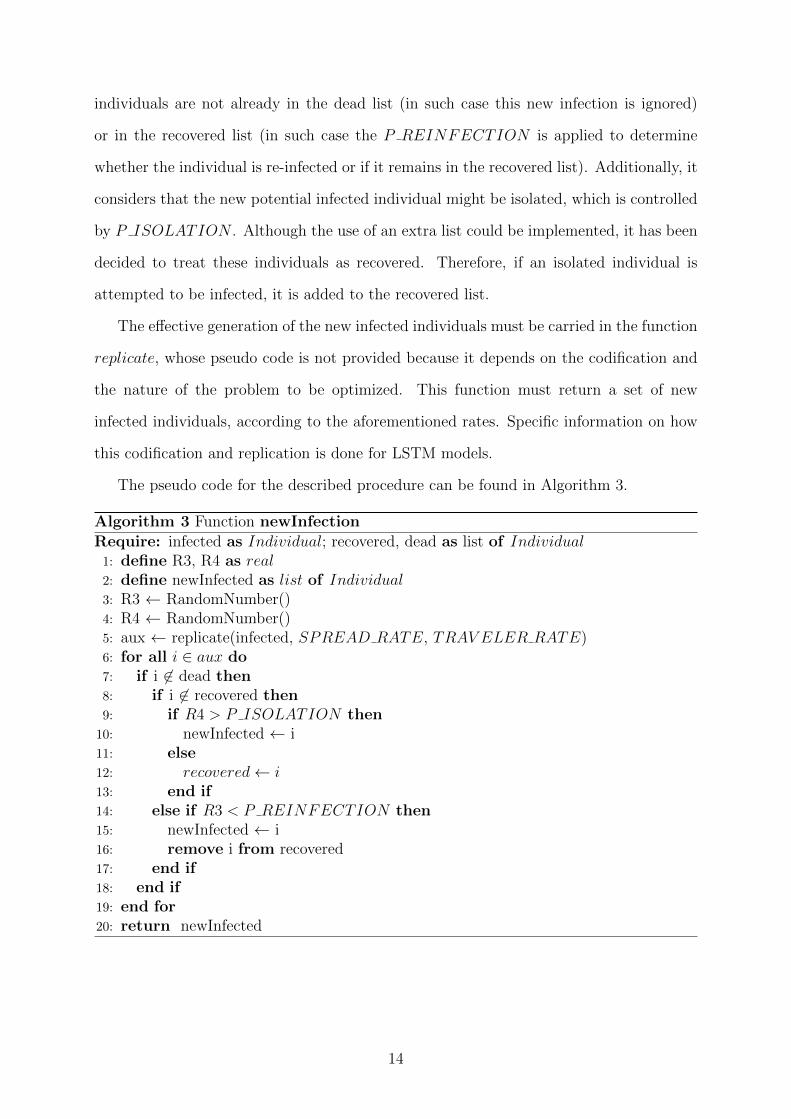
individuals are not already in the dead list (in such case this new infection is ignored)

or in the recovered list (in such case the P REINFECTION is applied to determine

whether the individual is re-infected or if it remains in the recovered list). Additionally, it

considers that the new potential infected individual might be isolated, which is controlled

by P ISOLATION . Although the use of an extra list could be implemented, it has been

decided to treat these individuals as recovered. Therefore, if an isolated individual is

attempted to be infected, it is added to the recovered list.

The effective generation of the new infected individuals must be carried in the function

replicate, whose pseudo code is not provided because it depends on the codification and

the nature of the problem to be optimized. This function must return a set of new

infected individuals, according to the aforementioned rates. Specific information on how

this codification and replication is done for LSTM models.

The pseudo code for the described procedure can be found in Algorithm 3.

Algorithm 3 Function newInfection

Require: infected as Individual; recovered, dead as list of Individual1: define R3, R4 as real2: define newInfected as list of Individual3: R3 ← RandomNumber()4: R4 ← RandomNumber()5: aux ← replicate(infected, SPREAD RATE, TRAV ELER RATE)6: for all i ∈ aux do7: if i 6∈ dead then8: if i 6∈ recovered then9: if R4 > P ISOLATION then

10: newInfected ← i11: else12: recovered← i13: end if14: else if R3 < P REINFECTION then15: newInfected ← i16: remove i from recovered17: end if18: end if19: end for20: return newInfected

14

3.4.4 Function die

This function is called from the main function. It evaluates all individuals in the infected

population and determines whether they die or not, according to the given PDIE. Those

meeting this condition, are sent to the dead list. Algorithm 4 describes this procedure.

Algorithm 4 Function die

Require: infectedPopulation as list of Individual1: define dead as list of Individual2: define R5 as real3: for all i ∈ infectedPopulation do4: R5 ← RandomNumber()5: if R5 < P DIE then6: dead ← i7: end if8: end for9: return dead

3.4.5 Function selectBestIndividual

This is an auxiliary function used to find the best fitness in a list of infected individuals.

Its peudo code is shown in Algorithm 5.

Algorithm 5 Function selectBestIndividual

Require: infectedPopulation as list of Individual1: define bestIndividual as Individual2: define bestFitness as real3: bestFitness ← MINV ALUE4: for all i ∈ infectedPopulation do5: if fitness(i) > bestFitness then6: bestFitness ← fitness(i)7: bestIndividual ← i8: end if9: end for

10: return bestIndividual

4 Hybridizing deep learning with CVOA

This section describes the codification proposed for an individual, in order to hybridize

deep learning with CVOA. The term hybridize is used in this context as the combination of

15

two computational techniques (deep learning and CVOA) so that the best hyperparameter

values are discovered. This strategy is very common in machine learning for optimizing

models during the training process [4, 7, 10].

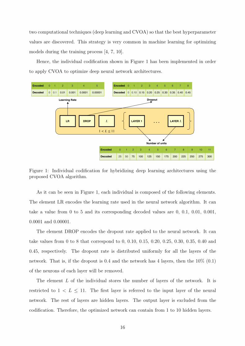
Hence, the individual codification shown in Figure 1 has been implemented in order

to apply CVOA to optimize deep neural network architectures.

Encoded 0 1 2 3 4 5

Decoded 0 0.1 0.01 0.001 0.0001 0.00001

Learning Rate

LR DROP

Encoded 0 1 2 3 4 5 6 7 8

Decoded 0 0.10 0.15 0.20 0.25 0.30 0.35 0.40 0.45

Dropout

Encoded 0 1 2 3 4 5 6 7 8 9 10 11

Decoded 25 50 75 100 125 150 175 200 225 250 275 300

Number of units

𝐿 LAYER 1 LAYER 𝐿. . .

1 < 𝐿 ≤ 11

Figure 1: Individual codification for hybridizing deep learning architectures using theproposed CVOA algorithm.

As it can be seen in Figure 1, each individual is composed of the following elements.

The element LR encodes the learning rate used in the neural network algorithm. It can

take a value from 0 to 5 and its corresponding decoded values are 0, 0.1, 0.01, 0.001,

0.0001 and 0.00001.

The element DROP encodes the dropout rate applied to the neural network. It can

take values from 0 to 8 that correspond to 0, 0.10, 0.15, 0.20, 0.25, 0.30, 0.35, 0.40 and

0.45, respectively. The dropout rate is distributed uniformly for all the layers of the

network. That is, if the dropout is 0.4 and the network has 4 layers, then the 10% (0.1)

of the neurons of each layer will be removed.

The element L of the individual stores the number of layers of the network. It is

restricted to 1 < L ≤ 11. The first layer is referred to the input layer of the neural

network. The rest of layers are hidden layers. The output layer is excluded from the

codification. Therefore, the optimized network can contain from 1 to 10 hidden layers.

16

The proposed individual codification has a variable size. Thus, its size depends on the

number of layers indicated in the element L. Consequently, a list of elements (LAYER

1, ..., LAYER L) are also included in the individual, which encode the number of units

(neurons) for each network layer. Each of these elements can take values from 0 to 11,

and their corresponding decoded values range from 25 to 300, with a step of 25.

4.1 PZ generation

The PZ, as it has been described previously, is the individual of the first iteration in the

CVOA algorithm. Following the hybridization proposed, a random individual is created

considering the codification defined above.

In first place, a random value for the learning rate of the PZ is generated. Specifically,

a number between 0 and 5 is generated randomly in a uniform distribution. Such limits

are indicated in Figure 1, according to the possible encoded values of the learning rate

element. The same process is carried out to produce a random value for the dropout

element. In such case, a random number between 0 and 8 is generated.

In second place, a random number of layers is generated for the element L of PZ.

Such number of layers is a random number between 2 and 11. Note that the first layer is

reserved for the input layer of the neural network, as it has been discussed before.

In last place, for each one of the L layers, a random number of units is generated

between 0 and 11, covering the possible encoded values for the number of units previously

defined (see Figure 1).

4.2 Infection procedure

The infection procedure described here corresponds to the functionality of replicate(),

introduced in the line 4 of the Algorithm 3. This procedure takes an individual as input

and returns an infected individual according to the following procedure.

The first step is to determine the element L of the infected individual that will be

mutated. The probability of such mutation occurs has been set to 13

so that every element

has the same probability to mutate. If the mutation occurs, then the element L of the

17

individual is modified according to the process described in Section 4.4.

If the element L (the number of layers of the network) changes, then the elements

encoding the different layers within the individual (LAYER 1, ..., LAYER L) must be

resized accordingly. Such resizing process is explained in Section 4.3.

The second step is to determine how many elements of the individual will be infected.

If the TRAV ELER RATE < 0, then the number of infected elements is generated

randomly from 0 to the length of the individual (excluding the element L). Else, the

TRAV ELER RATE indicates itself the number of infected elements.

As third step, once it is determined the number of infected elements of the individual,

a list of random positions is generated. For example, if three positions of the individual

must be changed, then the random positions affected could be, for instance, whose referred

to the elements {DROP, LAYER 2, LAYER 4}.

Finally, the selected positions of the individual are mutated. Such mutation is de-

scribed in Section 4.4.

4.3 Individual resizing process

When an individual is infected at the position of the element L, the list of elements

that encodes the number of units per layer (LAYER 1, ..., LAYER L) must be resized

accordingly.

In the case that the new number of layers after the infection is lower than its previous

value, then the last leftover elements are removed. For instance, if the initial individual is

{2, 0, 4}{3, 2, 1, 6} (four layers), the element L = 4 is infected and the new value is L = 2,

then the resulting individual will be {2, 0, 2}{3, 2}.

In the case that the new number of layers after the infection is higher than its previous

value, the new random elements are added at the end of the individual. For instance, if

the initial individual is {2, 0, 4}{3, 2, 1, 6} (four layers), the element L = 4 is infected and

the new value is L = 6, then the resulting individual could be {2, 0, 6}{3, 2, 1, 6, 0, 4}.

18

4.4 Single position mutation

The process carried out to change the value of a specific element of an individual is

described in this section.

First, a signed change amount C ∈ {−2,−1,+1,+2} is randomly determined using

the following criteria. A random real number P between 0 and 1 is generated using a

uniform distribution. If P < 0.25, then the change amount will be C = −2. Else if

P < 0.5, then the change amount will be C = −1. Else if P < 0.75, then the change

amount will be C = +1. Else, the change amount will be C = +2.

Once the amount of change is determined, the new value for the infected element is

computed. If its previous value is V , then the new value after the single position mutation

will be V ′ = V + C. If the new value V ′ exceeds the limits defined for the individual

codification, such value is set to the maximum or minimum allowed value accordingly.

5 CVOA preliminary analysis

This section provides an overview on how populations evolve over time, and how the

search space is explored to reach the optimum value for a given fitness function.

To conduct this experimentation, a simple binary codification has been used. The

fitness function was f(x) = (x − 15)2 because to goal of this section is to evaluate the

growth of the new infected populations, and not to the find challenging optimum values.

This function reaches the minimum value at x = 15, that is, f(15) = 0.

For this reason, individuals with 10, 20, 30, 40 and 50 bits have been tested. Tables 1-5

summarize the results achieved for each of these lengths, respectively. Every experiment

has been launched 50 times, determining that, on average, the optimum value was found

for 11, 12, 14, 15 and 17 iterations, respectively. Each table shows the results of an

execution meeting this criterion.

Table 6 summarizes the amount of search space explored, on average, before finding

the optimum value. For a small space of 210 = 1024 possible values, the optimum one is

reached after exploring 15.6250% valid solutions. However, this value acutely decreases as

19

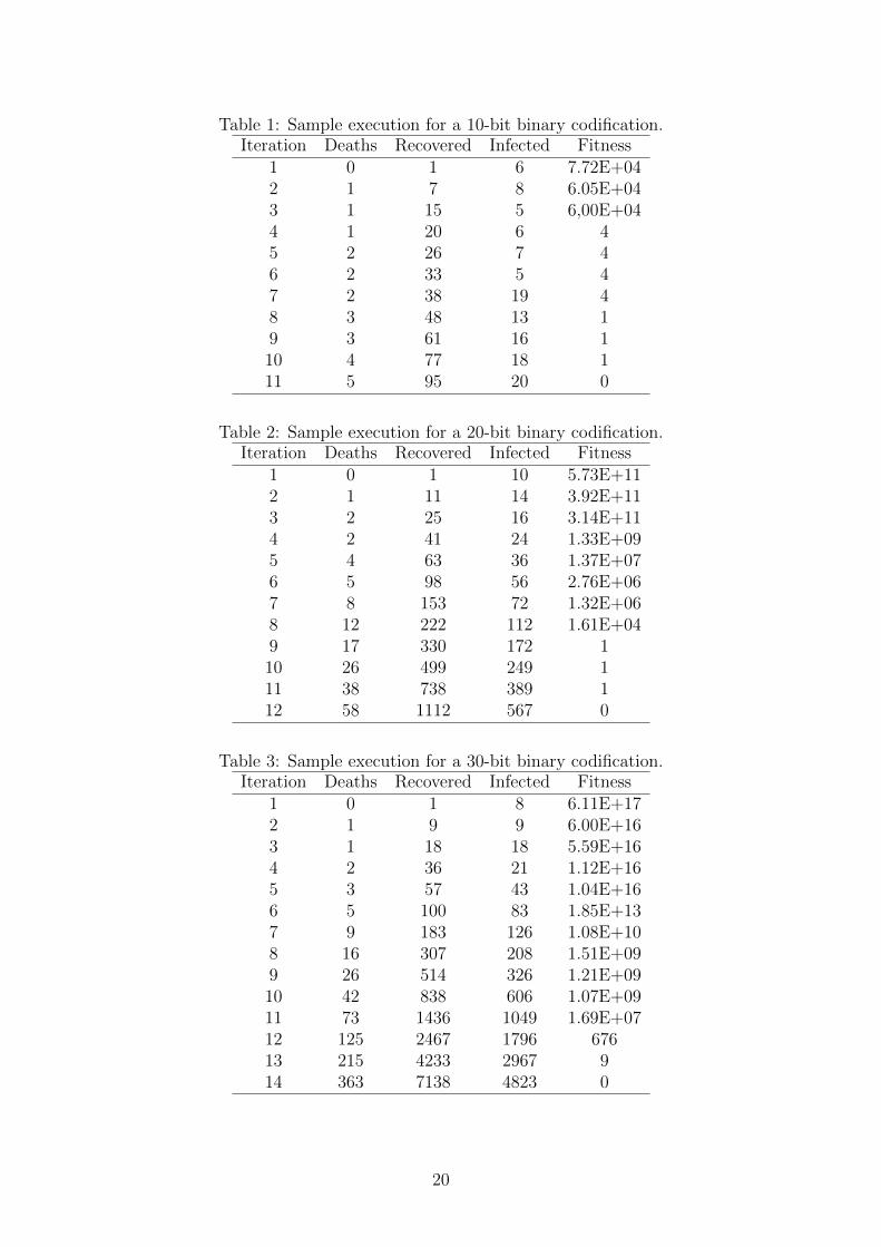
Table 1: Sample execution for a 10-bit binary codification.Iteration Deaths Recovered Infected Fitness

1 0 1 6 7.72E+042 1 7 8 6.05E+043 1 15 5 6,00E+044 1 20 6 45 2 26 7 46 2 33 5 47 2 38 19 48 3 48 13 19 3 61 16 110 4 77 18 111 5 95 20 0

Table 2: Sample execution for a 20-bit binary codification.Iteration Deaths Recovered Infected Fitness

1 0 1 10 5.73E+112 1 11 14 3.92E+113 2 25 16 3.14E+114 2 41 24 1.33E+095 4 63 36 1.37E+076 5 98 56 2.76E+067 8 153 72 1.32E+068 12 222 112 1.61E+049 17 330 172 110 26 499 249 111 38 738 389 112 58 1112 567 0

Table 3: Sample execution for a 30-bit binary codification.Iteration Deaths Recovered Infected Fitness

1 0 1 8 6.11E+172 1 9 9 6.00E+163 1 18 18 5.59E+164 2 36 21 1.12E+165 3 57 43 1.04E+166 5 100 83 1.85E+137 9 183 126 1.08E+108 16 307 208 1.51E+099 26 514 326 1.21E+0910 42 838 606 1.07E+0911 73 1436 1049 1.69E+0712 125 2467 1796 67613 215 4233 2967 914 363 7138 4823 0

20

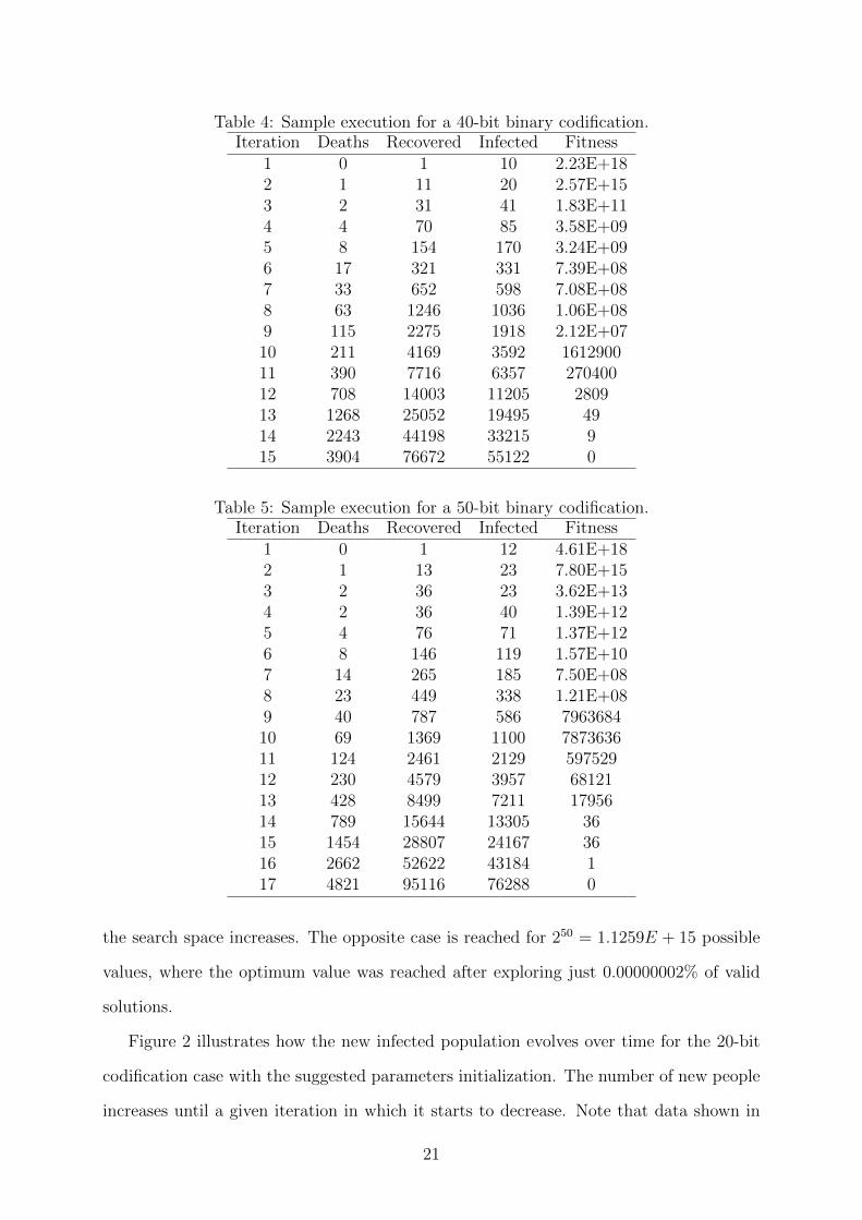
Table 4: Sample execution for a 40-bit binary codification.Iteration Deaths Recovered Infected Fitness

1 0 1 10 2.23E+182 1 11 20 2.57E+153 2 31 41 1.83E+114 4 70 85 3.58E+095 8 154 170 3.24E+096 17 321 331 7.39E+087 33 652 598 7.08E+088 63 1246 1036 1.06E+089 115 2275 1918 2.12E+0710 211 4169 3592 161290011 390 7716 6357 27040012 708 14003 11205 280913 1268 25052 19495 4914 2243 44198 33215 915 3904 76672 55122 0

Table 5: Sample execution for a 50-bit binary codification.Iteration Deaths Recovered Infected Fitness

1 0 1 12 4.61E+182 1 13 23 7.80E+153 2 36 23 3.62E+134 2 36 40 1.39E+125 4 76 71 1.37E+126 8 146 119 1.57E+107 14 265 185 7.50E+088 23 449 338 1.21E+089 40 787 586 796368410 69 1369 1100 787363611 124 2461 2129 59752912 230 4579 3957 6812113 428 8499 7211 1795614 789 15644 13305 3615 1454 28807 24167 3616 2662 52622 43184 117 4821 95116 76288 0

the search space increases. The opposite case is reached for 250 = 1.1259E + 15 possible

values, where the optimum value was reached after exploring just 0.00000002% of valid

solutions.

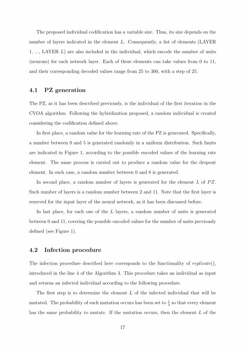
Figure 2 illustrates how the new infected population evolves over time for the 20-bit

codification case with the suggested parameters initialization. The number of new people

increases until a given iteration in which it starts to decrease. Note that data shown in

21

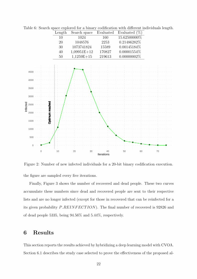
Table 6: Search space explored for a binary codification with different individuals length.Length Search space Evaluated Evaluated (%)

10 1024 160 15.62500000%20 1048576 2253 0.21486282%30 1073741824 15589 0.00145184%40 1,09951E+12 170827 0.00001554%50 1,1259E+15 219613 0.00000002%

●

●

●

●

●●

●

●

●

●

●●

●● ● ●

Opt

imum

rea

ched

Opt

imum

rea

ched

Opt

imum

rea

ched

Opt

imum

rea

ched

Opt

imum

rea

ched

Opt

imum

rea

ched

Opt

imum

rea

ched

Opt

imum

rea

ched

Opt

imum

rea

ched

Opt

imum

rea

ched

Opt

imum

rea

ched

Opt

imum

rea

ched

Opt

imum

rea

ched

Opt

imum

rea

ched

Opt

imum

rea

ched

Opt

imum

rea

ched

0

500

1000

1500

2000

2500

3000

3500

4000

4500

0 10 20 30 40 50 60 70Iterations

Infe

cted

Figure 2: Number of new infected individuals for a 20-bit binary codification execution.

the figure are sampled every five iterations.

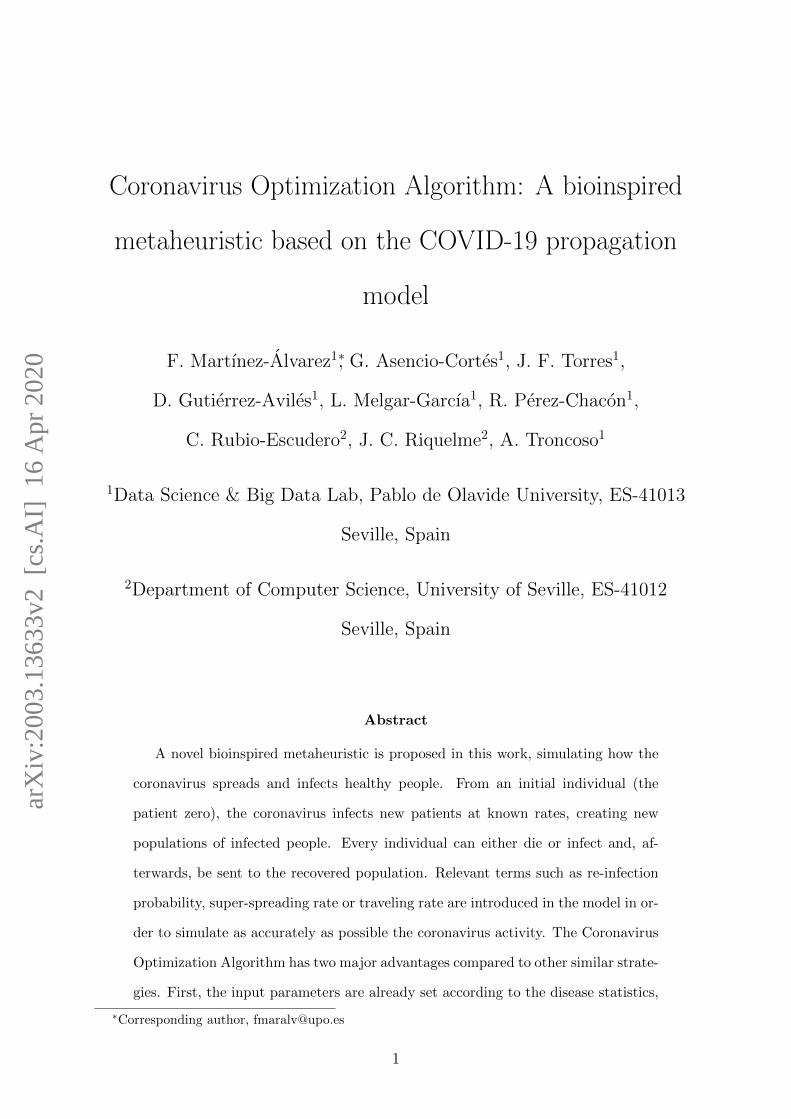
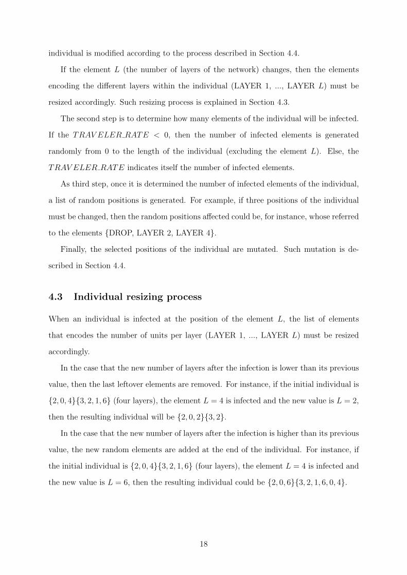
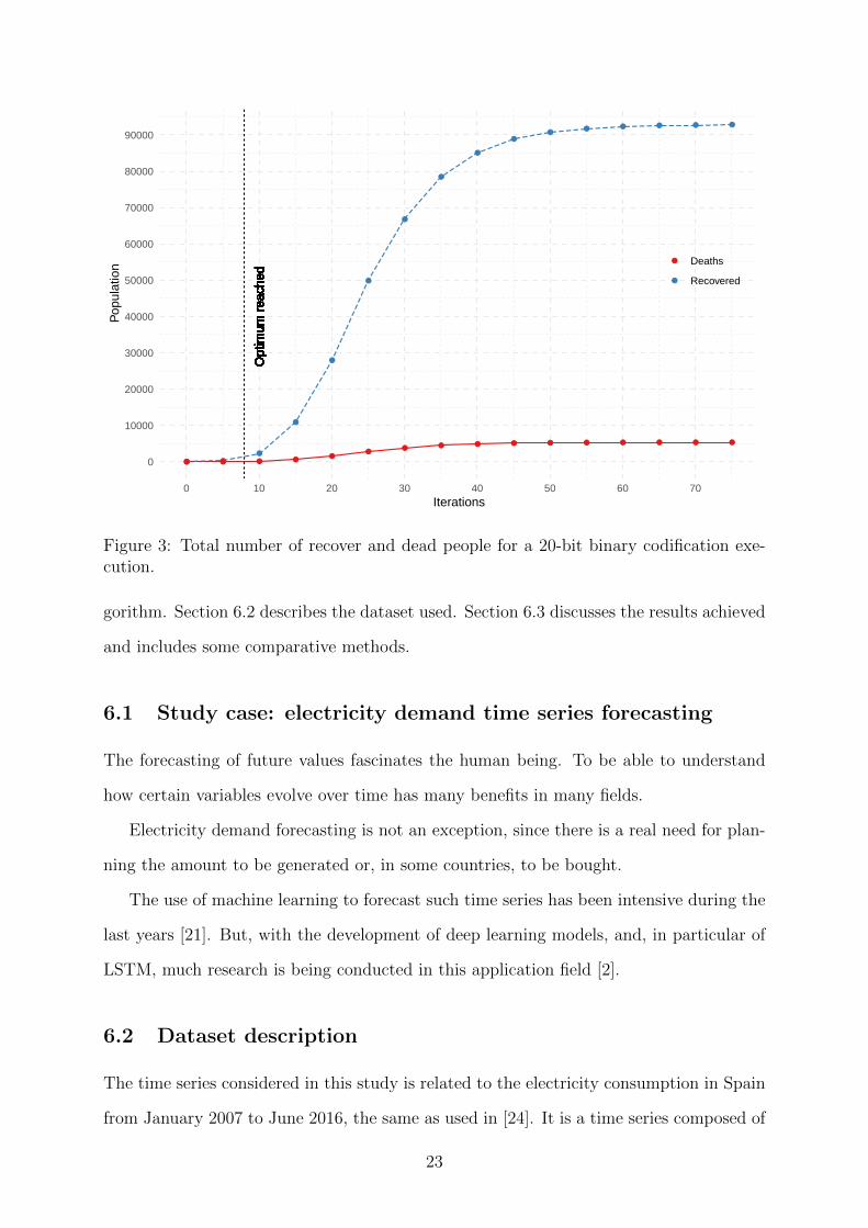
Finally, Figure 3 shows the number of recovered and dead people. These two curves

accumulate these numbers since dead and recovered people are sent to their respective

lists and are no longer infected (except for those in recovered that can be reinfected for a

its given probability P REINFECTION). The final number of recovered is 92826 and

of dead people 5335, being 94.56% and 5.44%, respectively.

6 Results

This section reports the results achieved by hybridizing a deep learning model with CVOA.

Section 6.1 describes the study case selected to prove the effectiveness of the proposed al-

22

● ●

●

●

●

●

●

●

●

●●

● ● ● ● ●

● ● ● ●●

●● ● ● ● ● ● ● ● ● ●

Opt

imum

rea

ched

Opt

imum

rea

ched

Opt

imum

rea

ched

Opt

imum

rea

ched

Opt

imum

rea

ched

Opt

imum

rea

ched

Opt

imum

rea

ched

Opt

imum

rea

ched

Opt

imum

rea

ched

Opt

imum

rea

ched

Opt

imum

rea

ched

Opt

imum

rea

ched

Opt

imum

rea

ched

Opt

imum

rea

ched

Opt

imum

rea

ched

Opt

imum

rea

ched

Opt

imum

rea

ched

Opt

imum

rea

ched

Opt

imum

rea

ched

Opt

imum

rea

ched

Opt

imum

rea

ched

Opt

imum

rea

ched

Opt

imum

rea

ched

Opt

imum

rea

ched

Opt

imum

rea

ched

Opt

imum

rea

ched

Opt

imum

rea

ched

Opt

imum

rea

ched

Opt

imum

rea

ched

Opt

imum

rea

ched

Opt

imum

rea

ched

Opt

imum

rea

ched

0

10000

20000

30000

40000

50000

60000

70000

80000

90000

0 10 20 30 40 50 60 70Iterations

Pop

ulat

ion

●

●

Deaths

Recovered

Figure 3: Total number of recover and dead people for a 20-bit binary codification exe-cution.

gorithm. Section 6.2 describes the dataset used. Section 6.3 discusses the results achieved

and includes some comparative methods.

6.1 Study case: electricity demand time series forecasting

The forecasting of future values fascinates the human being. To be able to understand

how certain variables evolve over time has many benefits in many fields.

Electricity demand forecasting is not an exception, since there is a real need for plan-

ning the amount to be generated or, in some countries, to be bought.

The use of machine learning to forecast such time series has been intensive during the

last years [21]. But, with the development of deep learning models, and, in particular of

LSTM, much research is being conducted in this application field [2].

6.2 Dataset description

The time series considered in this study is related to the electricity consumption in Spain

from January 2007 to June 2016, the same as used in [24]. It is a time series composed of

23

9 years and 6 months with a 10-minute sampling frequency, resulting in 497832 measures.

As in the original paper, the prediction horizon is 24, that is, this is a multi-step

strategy with h = 24. The size of samples used for the prediction of these 24 values is

168. Furthermore, the dataset was split into 70% for the training set and 30% for the test

set, and in addition, a 30% of the training set has also been selected for the validation set,

in order to find the optimal parameters. The training set covers the period from January

1, 2007 at 00:00 to August 20, 2013 at 02:40. Therefore, the test set comprises the period

from August 20, 2013 at 02:50 to June 21, 2016 at 23:40.

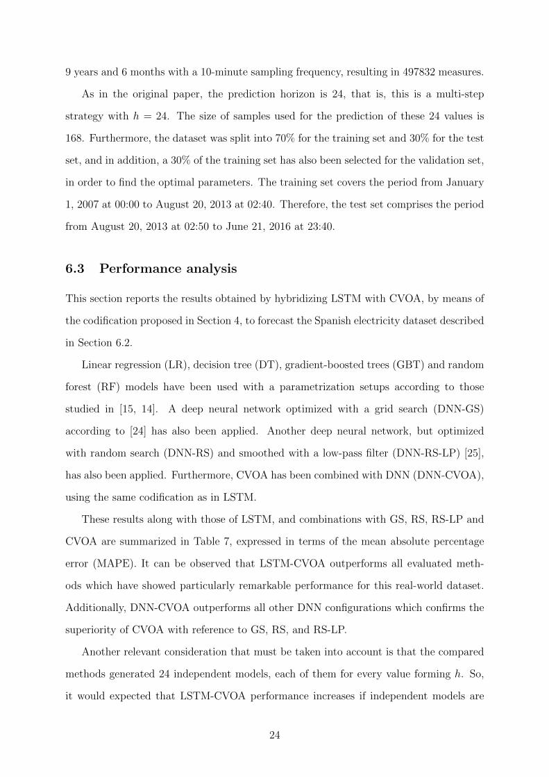
6.3 Performance analysis

This section reports the results obtained by hybridizing LSTM with CVOA, by means of

the codification proposed in Section 4, to forecast the Spanish electricity dataset described

in Section 6.2.

Linear regression (LR), decision tree (DT), gradient-boosted trees (GBT) and random

forest (RF) models have been used with a parametrization setups according to those

studied in [15, 14]. A deep neural network optimized with a grid search (DNN-GS)

according to [24] has also been applied. Another deep neural network, but optimized

with random search (DNN-RS) and smoothed with a low-pass filter (DNN-RS-LP) [25],

has also been applied. Furthermore, CVOA has been combined with DNN (DNN-CVOA),

using the same codification as in LSTM.

These results along with those of LSTM, and combinations with GS, RS, RS-LP and

CVOA are summarized in Table 7, expressed in terms of the mean absolute percentage

error (MAPE). It can be observed that LSTM-CVOA outperforms all evaluated meth-

ods which have showed particularly remarkable performance for this real-world dataset.

Additionally, DNN-CVOA outperforms all other DNN configurations which confirms the

superiority of CVOA with reference to GS, RS, and RS-LP.

Another relevant consideration that must be taken into account is that the compared

methods generated 24 independent models, each of them for every value forming h. So,

it would expected that LSTM-CVOA performance increases if independent models are

24

generated for each of the values in h.

Table 7: Results in terms of MAPE for CVOA-LSTM compared to other well establishedmethods.

Method MAPE (%)LR 7.34DT 2.88GBT 2.72RF 2.20DNN-GS 1.68DNN-RS 1.57DNN-RS-LP 1.36DNN-CVOA 1.18LSTM-GS 1.22LSTM-RS 0.84LSTM-RS-LP 0.82LSTM-CVOA 0.47

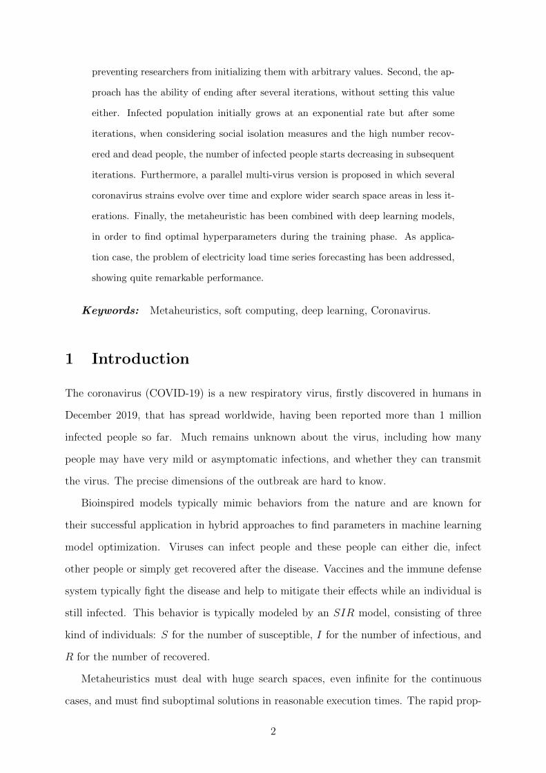
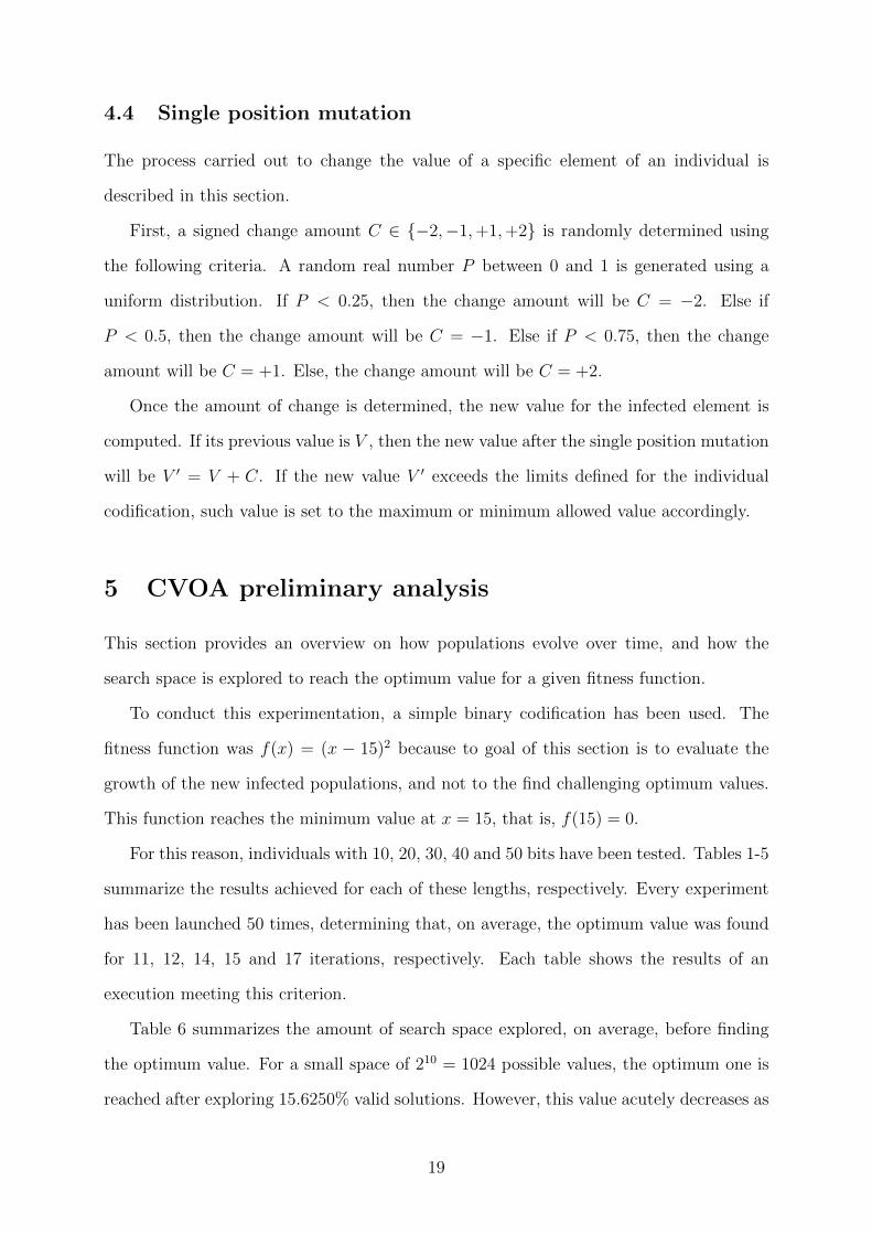
These results have been achieved with the individual {4, 0, 8}{9, 7, 2, 7, 2, 7, 10, 7},

which decoded involves the following architecture parameters:

• Learning rate: 10E-04.

• Dropout: 0.

• Number of layers: 8.

• Units per layer: [250, 200, 75, 200, 75, 200, 275, 200]

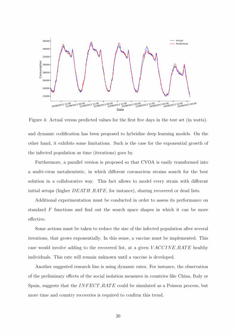
Finally, Figure 4 depicts the first five predicted days versus their actual values, ex-

pressed in watts.

7 Conclusions and future works

This work has introduced a novel bioinspired metaheuristic, based on the coronavirus

behavior. On the one hand, CVOA has two major advantages. First, its highly relation

to the coronavirus spreading model, prevents the authors to make any decision about the

inputs’ values. Second, it ends after a certain number of iterations due to the exchange

of individuals between healthy and dead/recovered lists. Additionally, a novel discrete

25

20/08/2013 12:0021/08/2013 00:00

21/08/2013 12:0022/08/2013 00:00

22/08/2013 12:0023/08/2013 00:00

23/08/2013 12:0024/08/2013 00:00

24/08/2013 12:0025/08/2013 00:00

Date

22000

24000

26000

28000

30000

32000

34000

36000Co

nsum

ptio

nActualPredictions

Figure 4: Actual versus predicted values for the first five days in the test set (in watts).

and dynamic codification has been proposed to hybridize deep learning models. On the

other hand, it exhibits some limitations. Such is the case for the exponential growth of

the infected population as time (iterations) goes by.

Furthermore, a parallel version is proposed so that CVOA is easily transformed into

a multi-virus metaheuristic, in which different coronavirus strains search for the best

solution in a collaborative way. This fact allows to model every strain with different

initial setups (higher DEATH RATE, for instance), sharing recovered or dead lists.

Additional experimentation must be conducted in order to assess its performance on

standard F functions and find out the search space shapes in which it can be more

effective.

Some actions must be taken to reduce the size of the infected population after several

iterations, that grows exponentially. In this sense, a vaccine must be implemented. This

case would involve adding to the recovered list, at a given V ACCINE RATE healthy

individuals. This rate will remain unknown until a vaccine is developed.

Another suggested research line is using dynamic rates. For instance, the observation

of the preliminary effects of the social isolation measures in countries like China, Italy or

Spain, suggests that the INFECT RATE could be simulated as a Poisson process, but

more time and country recoveries is required to confirm this trend.

26

Finally, for the multi-step forecasting problem analyzed, it would be desirable to gen-

erate independent models for each of the values that form the prediction horizon h.

Supplementary material

Along with this paper, an academic version in Java for a binary codification is provided,

with a simple fitness function (https://github.com/DataLabUPO/CVOA_academic). Ad-

ditionally, the code in Phyton for the deep learning approach is also provided, with a more

complex codification and the suggested implementation, according to the pseudocode pro-

vided (https://github.com/DataLabUPO/CVOA_LSTM).

Acknowledgments

The authors would like to thank the Spanish Ministry of Economy and Competitiveness

for the support under project TIN2017-88209-C2.

References

[1] World Health Organization. https://www.who.int/es/emergencies/diseases/

novel-coronavirus-2019. Accessed: 2020-03-20.

[2] J. Bedi and D. Toshniwal. Deep learning framework to forecast electricity demand.

Applied Energy, 238:1312–1326, 2019.

[3] A. Bosire. Recurrent Neural Network Training using ABC Algorithm for Traffic

Volume Prediction. Informatica, 43:551–559, 2019.

[4] L. Calvet, J.D. Armas, D. Masip, and A. A. Juan. Learnheuristics: Hybridizing meta-

heuristics with machine learning for optimization with dynamic inputs. Mathematics

Open, 15:261–280, 2017.

27

[5] J. Chen, H. Xing, H. Yang, and L. Xu. Network Traffic Prediction Based on LSTM

Networks with Genetic Algorithm. Lecture Notes in Electrical Engineering, 550:411–

419, 2019.

[6] H. Chung and K.-S. Shin. Genetic Algorithm-Optimized Long Short-Term Memory

Network for Stock Market Prediction. Sustainability, 10(10):3765, 2018.

[7] A. Darwish, A. E. Hassanien, and S. Das. A survey of swarm and evolutionary

computing approaches for deep learning. Artificial Intelligence Review, 53(3):1767–

1812, 2020.

[8] S. De-Cnudde, Y. Ramon, D. Martens, and F. Provost. Deep learning on big, sparse,

behavioral data. Big Data, 7(4):286–307, 2019.

[9] T. Desell, S. Clachar, J. Higgins, and B. Wild. Evolving deep recurrent neural

networks using ant colony optimization. Lecture Notes in Computer Science, 9026:86–

98, 2015.

[10] D. Devikanniga, K. Vetrivel, and N. Badrinath. Review of meta-heuristic optimiza-

tion based artificial neural networks and its applications. Journal of Physics: Con-

ference Series, 1362(1):012074, 2019.

[11] V. Dhar, C. Sun, and P. Batra. Transforming Finance Into Vision: Concurrent

Financial Time Series as Convolutional Net. Big Data, 7(4):276–285, 2019.

[12] A. ElSaid, F. ElJamiy, J. Higgings, B. Wild, B. Wild, and T. Desell. Using ant

colony optimization to optimize long short-term memory recurrent neural networks.

In Proceedings of the Genetic and Evolutionary Computation Conference, pages 13–

20, 2018.

[13] F. E. Fernandes-Junior and G. G. Yen. Particle swarm optimization of deep neural

networks architectures for image classification. Swarm and Evolutionary Computa-

tion, 49:62–74, 2019.

28

[14] A. Galicia, R. L. Talavera-Llames, A. Troncoso, I. Koprinska, and F. Martınez-

Alvarez. Multi-step forecasting for big data time series based on ensemble learning.

Knowledge-Based Systems, 163:830–841, 2019.

[15] A. Galicia, J. F. Torres, F. Martınez-Alvarez, and A. Troncoso. Scalable forecasting

techniques applied to big electricity time series. Lecture Notes in Computer Science,

10306:165–175, 2019.

[16] F. Glover and G. A. Kochenberger. Handbook of metaheuristics. Springer, 2003.

[17] A. Kelotra and P. Pandey. Stock Market Prediction Using Optimized Deep-

ConvLSTM Model. Big Data, 8(1):5–24, 2020.

[18] Y. C. Liang and J. R. Cuevas-Juarez. A novel metaheuristic for continuous optimiza-

tion problems: Virus optimization algorithm. Engineering Optimization, 48(1):73–93,

2016.

[19] Y. C. Liang and J. R. Cuevas-Juarez. A self-adaptive virus optimization algorithm

for continuous optimization problems. Soft Computing, In press, 2020.

[20] Zhao Liu, Xincheng Sun, Shuai Wang, Mengjiao Pan, Yue Zhang, and Zhendong Ji.

Midterm power load forecasting model based on kernel principal component analysis

and back propagation neural network with particle swarm optimization. Big Data,

7(2):130–138, 2019.

[21] F. Martınez-Alvarez, A. Troncoso, G. Asencio-Cortes, and J. C. Riquelme. A sur-

vey on data mining techniques applied to electricity-related time series forecasting.

Energies, 8(11):13162–13193, 2015.

[22] N. M. Nawi, A. Khan, and M. Z. Rehman. A New Optimized Cuckoo Search Recur-

rent Neural Network (CSRNN). In Proceedings of the International Conference on

Robotic, Vision, Signal Processing & Power Applications, pages 335–341, 2014.

29

[23] D. Srivastava, Y. Singh, and A. Sahoo. Auto Tuning of RNN Hyper-parameters

using Cuckoo Search Algorithm. In Proceedings of the International Conference on

Contemporary Computing, pages 1–5, 2019.

[24] J. F. Torres, A. Galicia, A. Troncoso, and F. Martınez-Alvarez. A scalable approach

based on deep learning for big data time series forecasting. Integrated Computer-

Aided Engineering, 25(4):335–348, 2018.

[25] J. F. Torres, D. Gutierrez-Aviles, A. Troncoso, and F. Martınez-Alvarez. Random

hyper-parameter search-based deep neural network for power consumption forecast-

ing. Lecture Notes in Computer Science, 11506:259–269, 2019.

[26] A. D. Yuliyono and A. S. Girsang. Artificial Bee Colony-Optimized LSTM for Bitcoin

Price Prediction. Advances in Science, Technology and Engineering Systems Journal,

4(5):375–383, 2019.

30