Embed Size (px)
Citation preview

Journal of Machine Learning Research 14 (2013) 3207-3260 Submitted 9/12; Revised 3/13; Published 11/13
Counterfactual Reasoning and Learning Systems: The Example ofComputational Advertising
Léon Bottou [email protected] Microsoft WayRedmond, WA 98052, USA
Jonas Peters∗ [email protected] Planck InstituteSpemannstraße 3872076 Tübingen, Germany
Joaquin Quiñonero-Candela† [email protected]
Denis X. Charles [email protected]
D. Max Chickering [email protected]
Elon Portugaly [email protected]
Dipankar Ray [email protected]
Patrice Simard [email protected]
Ed Snelson [email protected]
Microsoft1 Microsoft WayRedmond, WA 98052, USA
AbstractThis work shows how to leverage causal inference to understand the behavior of complex learningsystems interacting with their environment and predict the consequences of changes to the sys-tem. Such predictions allow both humans and algorithms to select the changes that would haveimproved the system performance. This work is illustrated by experiments on the ad placementsystem associated with the Bing search engine.Keywords: causation, counterfactual reasoning, computational advertising
1. Introduction
Statistical machine learning technologies in the real world are never without a purpose. Using theirpredictions, humans or machines make decisions whose circuitous consequences often violate themodeling assumptions that justified the system design in the first place.
Such contradictions appear very clearly in the case of the learning systems that power webscale applications such as search engines, ad placement engines, or recommendation systems. Forinstance, the placement of advertisement on the result pages of Internet search engines depend onthe bids of advertisers and on scores computed by statistical machine learning systems. Becausethe scores affect the contents of the result pages proposed to the users, they directly influence theoccurrence of clicks and the corresponding advertiser payments. They also have important indirecteffects. Ad placement decisions impact the satisfaction of the users and therefore their willingnessto frequent this web site in the future. They also impact the return on investment observed by the
∗. Current address: Jonas Peters, ETH Zürich, Rämistraße 101, 8092 Zürich, Switzerland.†. Current address: Joaquin Quiñonero-Candela, Facebook, 1 Hacker Way, Menlo Park, CA 94025, USA.
c©2013 Léon Bottou, Jonas Peters, Joaquin Quiñonero-Candela, Denis X. Charles, D. Max Chickering, Elon Portugaly, Dipankar Ray,Patrice Simard and Ed Snelson

BOTTOU, PETERS, ET AL.
advertisers and therefore their future bids. Finally they change the nature of the data collected fortraining the statistical models in the future.
These complicated interactions are clarified by important theoretical works. Under simplifiedassumptions, mechanism design (Myerson, 1981) leads to an insightful account of the advertiserfeedback loop (Varian, 2007; Edelman et al., 2007). Under simplified assumptions, multiarmedbandits theory (Robbins, 1952; Auer et al., 2002; Langford and Zhang, 2008) and reinforcementlearning (Sutton and Barto, 1998) describe the exploration/exploitation dilemma associated withthe training feedback loop. However, none of these approaches gives a complete account of thecomplex interactions found in real-life systems.
This contribution proposes a novel approach: we view these complicated interactions as man-ifestations of the fundamental difference that separates correlation and causation. Using the adplacement example as a model of our problem class, we therefore argue that the language and themethods of causal inference provide flexible means to describe such complex machine learning sys-tems and give sound answers to the practical questions facing the designer of such a system. Isit useful to pass a new input signal to the statistical model? Is it worthwhile to collect and labela new training set? What about changing the loss function or the learning algorithm? In order toanswer such questions and improve the operational performance of the learning system, one needsto unravel how the information produced by the statistical models traverses the web of causes andeffects and eventually produces measurable performance metrics.
Readers with an interest in causal inference will find in this paper (i) a real world exampledemonstrating the value of causal inference for large-scale machine learning applications, (ii)causal inference techniques applicable to continuously valued variables with meaningful confidenceintervals, and (iii) quasi-static analysis techniques for estimating how small interventions affect cer-tain causal equilibria. Readers with an interest in real-life applications will find (iv) a selection ofpractical counterfactual analysis techniques applicable to many real-life machine learning systems.Readers with an interest in computational advertising will find a principled framework that (v) ex-plains how to soundly use machine learning techniques for ad placement, and (vi) conceptuallyconnects machine learning and auction theory in a compelling manner.
The paper is organized as follows. Section 2 gives an overview of the advertisement placementproblem which serves as our main example. In particular, we stress some of the difficulties encoun-tered when one approaches such a problem without a principled perspective. Section 3 provides acondensed review of the essential concepts of causal modeling and inference. Section 4 centers onformulating and answering counterfactual questions such as “how would the system have performedduring the data collection period if certain interventions had been carried out on the system ?” Wedescribe importance sampling methods for counterfactual analysis, with clear conditions of validityand confidence intervals. Section 5 illustrates how the structure of the causal graph reveals opportu-nities to exploit prior information and vastly improve the confidence intervals. Section 6 describeshow counterfactual analysis provides essential signals that can drive learning algorithms. Assumethat we have identified interventions that would have caused the system to perform well during thedata collection period. Which guarantee can we obtain on the performance of these same inter-ventions in the future? Section 7 presents counterfactual differential techniques for the study ofequlibria. Using data collected when the system is at equilibrium, we can estimate how a smallintervention displaces the equilibrium. This provides an elegant and effective way to reason aboutlong-term feedback effects. Various appendices complete the main text with information that wethink more relevant to readers with specific backgrounds.
3208

COUNTERFACTUAL REASONING AND LEARNING SYSTEMS
2. Causation Issues in Computational Advertising
After giving an overview of the advertisement placement problem, which serves as our main ex-ample, this section illustrates some of the difficulties that arise when one does not pay sufficientattention to the causal structure of the learning system.
2.1 Advertisement Placement
All Internet users are now familiar with the advertisement messages that adorn popular web pages.Advertisements are particularly effective on search engine result pages because users who aresearching for something are good targets for advertisers who have something to offer. Severalactors take part in this Internet advertisement game:
• Advertisers create advertisement messages, and place bids that describe how much they arewilling to pay to see their ads displayed or clicked.
• Publishers provide attractive web services, such as, for instance, an Internet search engine.They display selected ads and expect to receive payments from the advertisers. The infras-tructure to collect the advertiser bids and select ads is sometimes provided by an advertisingnetwork on behalf of its affiliated publishers. For the purposes of this work, we simply con-sider a publisher large enough to run its own infrastructure.
• Users reveal information about their current interests, for instance, by entering a query in asearch engine. They are offered web pages that contain a selection of ads (Figure 1). Userssometimes click on an advertisement and are transported to a web site controlled by the ad-vertiser where they can initiate some business.
A conventional bidding language is necessary to precisely define under which conditions an adver-tiser is willing to pay the bid amount. In the case of Internet search advertisement, each bid specifies(a) the advertisement message, (b) a set of keywords, (c) one of several possible matching criteriabetween the keywords and the user query, and (d) the maximal price the advertiser is willing topay when a user clicks on the ad after entering a query that matches the keywords according to thespecified criterion.
Whenever a user visits a publisher web page, an advertisement placement engine runs an auctionin real time in order to select winning ads, determine where to display them in the page, and computethe prices charged to advertisers, should the user click on their ad. Since the placement engineis operated by the publisher, it is designed to further the interests of the publisher. Fortunatelyfor everyone else, the publisher must balance short term interests, namely the immediate revenuebrought by the ads displayed on each web page, and long term interests, namely the future revenuesresulting from the continued satisfaction of both users and advertisers.
Auction theory explains how to design a mechanism that optimizes the revenue of the seller ofa single object (Myerson, 1981; Milgrom, 2004) under various assumptions about the informationavailable to the buyers regarding the intentions of the other buyers. In the case of the ad placementproblem, the publisher runs multiple auctions and sells opportunities to receive a click. When nearlyidentical auctions occur thousand of times per second, it is tempting to consider that the advertisershave perfect information about each other. This assumption gives support to the popular generalizedsecond price rank-score auction (Varian, 2007; Edelman et al., 2007):
3209
BOTTOU, PETERS, ET AL.
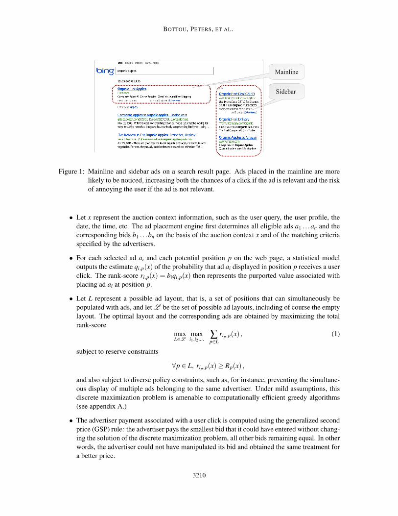
Figure 1: Mainline and sidebar ads on a search result page. Ads placed in the mainline are morelikely to be noticed, increasing both the chances of a click if the ad is relevant and the riskof annoying the user if the ad is not relevant.
• Let x represent the auction context information, such as the user query, the user profile, thedate, the time, etc. The ad placement engine first determines all eligible ads a1 . . .an and thecorresponding bids b1 . . .bn on the basis of the auction context x and of the matching criteriaspecified by the advertisers.
• For each selected ad ai and each potential position p on the web page, a statistical modeloutputs the estimate qi,p(x) of the probability that ad ai displayed in position p receives a userclick. The rank-score ri,p(x) = biqi,p(x) then represents the purported value associated withplacing ad ai at position p.
• Let L represent a possible ad layout, that is, a set of positions that can simultaneously bepopulated with ads, and let L be the set of possible ad layouts, including of course the emptylayout. The optimal layout and the corresponding ads are obtained by maximizing the totalrank-score
maxL∈L
maxi1,i2,...
∑p∈L
rip,p(x) , (1)
subject to reserve constraints
∀p ∈ L, rip,p(x)≥ Rp(x) ,
and also subject to diverse policy constraints, such as, for instance, preventing the simultane-ous display of multiple ads belonging to the same advertiser. Under mild assumptions, thisdiscrete maximization problem is amenable to computationally efficient greedy algorithms(see appendix A.)
• The advertiser payment associated with a user click is computed using the generalized secondprice (GSP) rule: the advertiser pays the smallest bid that it could have entered without chang-ing the solution of the discrete maximization problem, all other bids remaining equal. In otherwords, the advertiser could not have manipulated its bid and obtained the same treatment fora better price.
3210

COUNTERFACTUAL REASONING AND LEARNING SYSTEMS
Under the perfect information assumption, the analysis suggests that the publisher simply needs tofind which reserve prices Rp(x) yield the best revenue per auction. However, the total revenue of thepublisher also depends on the traffic experienced by its web site. Displaying an excessive numberof irrelevant ads can train users to ignore the ads, and can also drive them to competing web sites.Advertisers can artificially raise the rank-scores of irrelevant ads by temporarily increasing the bids.Indelicate advertisers can create deceiving advertisements that elicit many clicks but direct users tospam web sites. Experience shows that the continued satisfaction of the users is more important tothe publisher than it is to the advertisers.
Therefore the generalized second price rank-score auction has evolved. Rank-scores have beenaugmented with terms that quantify the user satisfaction or the ad relevance. Bids receive adaptivediscounts in order to deal with situations where the perfect information assumption is unrealistic.These adjustments are driven by additional statistical models. The ad placement engine shouldtherefore be viewed as a complex learning system interacting with both users and advertisers.
2.2 Controlled Experiments
The designer of such an ad placement engine faces the fundamental question of testing whethera proposed modification of the ad placement engine results in an improvement of the operationalperformance of the system.
The simplest way to answer such a question is to try the modification. The basic idea is torandomly split the users into treatment and control groups (Kohavi et al., 2008). Users from thecontrol group see web pages generated using the unmodified system. Users of the treatment groupssee web pages generated using alternate versions of the system. Monitoring various performancemetrics for a couple months usually gives sufficient information to reliably decide which variant ofthe system delivers the most satisfactory performance.
Modifying an advertisement placement engine elicits reactions from both the users and the ad-vertisers. Whereas it is easy to split users into treatment and control groups, splitting advertisersinto treatment and control groups demands special attention because each auction involves multi-ple advertisers (Charles et al., 2012). Simultaneously controlling for both users and advertisers isprobably impossible.
Controlled experiments also suffer from several drawbacks. They are expensive because theydemand a complete implementation of the proposed modifications. They are slow because each ex-periment typically demands a couple months. Finally, although there are elegant ways to efficientlyrun overlapping controlled experiments on the same traffic (Tang et al., 2010), they are limited bythe volume of traffic available for experimentation.
It is therefore difficult to rely on controlled experiments during the conception phase of potentialimprovements to the ad placement engine. It is similarly difficult to use controlled experiments todrive the training algorithms associated with click probability estimation models. Cheaper and fasterstatistical methods are needed to drive these essential aspects of the development of an ad placementengine. Unfortunately, interpreting cheap and fast data can be very deceiving.
2.3 Confounding Data
Assessing the consequence of an intervention using statistical data is generally challenging becauseit is often difficult to determine whether the observed effect is a simple consequence of the interven-tion or has other uncontrolled causes.
3211

BOTTOU, PETERS, ET AL.
Overall Patients withsmall stones
Patients withlarge stones
Treatment A:Open surgery 78% (273/350) 93% (81/87) 73% (192/263)
Treatment B:Percutaneous nephrolithotomy 83% (289/350) 87% (234/270) 69% (55/80)
Table 1: A classic example of Simpson’s paradox. The table reports the success rates of two treat-ments for kidney stones (Charig et al., 1986, Tables I and II). Although the overall successrate of treatment B seems better, treatment B performs worse than treatment A on bothpatients with small kidney stones and patients with large kidney stones. See Section 2.3.
For instance, the empirical comparison of certain kidney stone treatments illustrates this dif-ficulty (Charig et al., 1986). Table 2.3 reports the success rates observed on two groups of 350patients treated with respectively open surgery (treatment A, with 78% success) and percutaneousnephrolithotomy (treatment B, with 83% success). Although treatment B seems more successful, itwas more frequently prescribed to patients suffering from small kidney stones, a less serious con-dition. Did treatment B achieve a high success rate because of its intrinsic qualities or because itwas preferentially applied to less severe cases? Further splitting the data according to the size ofthe kidney stones reverses the conclusion: treatment A now achieves the best success rate for bothpatients suffering from large kidney stones and patients suffering from small kidney stones. Suchan inversion of the conclusion is called Simpson’s paradox (Simpson, 1951).
The stone size in this study is an example of a confounding variable, that is an uncontrolledvariable whose consequences pollute the effect of the intervention. Doctors knew the size of thekidney stones, chose to treat the healthier patients with the least invasive treatment B, and thereforecaused treatment B to appear more effective than it actually was. If we now decide to apply treat-ment B to all patients irrespective of the stone size, we break the causal path connecting the stonesize to the outcome, we eliminate the illusion, and we will experience disappointing results.
When we suspect the existence of a confounding variable, we can split the contingency tablesand reach improved conclusions. Unfortunately we cannot fully trust these conclusions unless weare certain to have taken into account all confounding variables. The real problem therefore comesfrom the confounding variables we do not know.
Randomized experiments arguably provide the only correct solution to this problem (see Stigler,1992). The idea is to randomly chose whether the patient receives treatment A or treatment B.Because this random choice is independent from all the potential confounding variables, knownand unknown, they cannot pollute the observed effect of the treatments (see also Section 4.2). Thisis why controlled experiments in ad placement (Section 2.2) randomly distribute users betweentreatment and control groups, and this is also why, in the case of an ad placement engine, weshould be somehow concerned by the practical impossibility to randomly distribute both users andadvertisers.
3212

COUNTERFACTUAL REASONING AND LEARNING SYSTEMS
Overall q2 low q2 high
q1 low 6.2% (124/2000) 5.1% (92/1823) 18.1% (32/176)
q1 high 7.5% (149/2000) 4.8% (71/1500) 15.6% (78/500)
Table 2: Confounding data in ad placement. The table reports the click-through rates and the clickcounts of the second mainline ad. The overall counts suggest that the click-through rateof the second mainline ad increases when the click probability estimate q1 of the top ad ishigh. However, if we further split the pages according to the click probability estimate q2of the second mainline ad, we reach the opposite conclusion. See Section 2.4.
2.4 Confounding Data in Ad Placement
Let us return to the question of assessing the value of passing a new input signal to the ad placementengine click prediction model. Section 2.1 outlines a placement method where the click probabilityestimates qi,p(x) depend on the ad and the position we consider, but do not depend on other adsdisplayed on the page. We now consider replacing this model by a new model that additionally usesthe estimated click probability of the top mainline ad to estimate the click probability of the secondmainline ad (Figure 1). We would like to estimate the effect of such an intervention using existingstatistical data.
We have collected ad placement data for Bing search result pages served during three consecu-tive hours on a certain slice of traffic. Let q1 and q2 denote the click probability estimates computedby the existing model for respectively the top mainline ad and the second mainline ad. After ex-cluding pages displaying fewer than two mainline ads, we form two groups of 2000 pages randomlypicked among those satisfying the conditions q1 < 0.15 for the first group and q1 ≥ 0.15 for thesecond group. Table 2.4 reports the click counts and frequencies observed on the second mainlinead in each group. Although the overall numbers show that users click more often on the secondmainline ad when the top mainline ad has a high click probability estimate q1, this conclusion isreversed when we further split the data according to the click probability estimate q2 of the secondmainline ad.
Despite superficial similarities, this example is considerably more difficult to interpret than thekidney stone example. The overall click counts show that the actual click-through rate of the secondmainline ad is positively correlated with the click probability estimate on the top mainline ad. Doesthis mean that we can increase the total number of clicks by placing regular ads below frequentlyclicked ads?
Remember that the click probability estimates depend on the search query which itself dependson the user intention. The most likely explanation is that pages with a high q1 are frequently asso-ciated with more commercial searches and therefore receive more ad clicks on all positions. Theobserved correlation occurs because the presence of a click and the magnitude of the click probabil-ity estimate q1 have a common cause: the user intention. Meanwhile, the click probability estimateq2 returned by the current model for the second mainline ad also depend on the query and thereforethe user intention. Therefore, assuming that this dependence has comparable strength, and assumingthat there are no other causal paths, splitting the counts according to the magnitude of q2 factors outthe effects of this common confounding cause. We then observe a negative correlation which now
3213

BOTTOU, PETERS, ET AL.
suggests that a frequently clicked top mainline ad has a negative impact on the click-through rate ofthe second mainline ad.
If this is correct, we would probably increase the accuracy of the click prediction model byswitching to the new model. This would decrease the click probability estimates for ads placed inthe second mainline position on commercial search pages. These ads are then less likely to clearthe reserve and therefore more likely to be displayed in the less attractive sidebar. The net resultis probably a loss of clicks and a loss of money despite the higher quality of the click probabilitymodel. Although we could tune the reserve prices to compensate this unfortunate effect, nothingin this data tells us where the performance of the ad placement engine will land. Furthermore,unknown confounding variables might completely reverse our conclusions.
Making sense out of such data is just too complex !
2.5 A Better Way
It should now be obvious that we need a more principled way to reason about the effect of potentialinterventions. We provide one such more principled approach using the causal inference machinery(Section 3). The next step is then the identification of a class of questions that are sufficiently ex-pressive to guide the designer of a complex learning system, and sufficiently simple to be answeredusing data collected in the past using adequate procedures (Section 4).
A machine learning algorithm can then be viewed as an automated way to generate questionsabout the parameters of a statistical model, obtain the corresponding answers, and update the param-eters accordingly (Section 6). Learning algorithms derived in this manner are very flexible: humandesigners and machine learning algorithms can cooperate seamlessly because they rely on similarsources of information.
3. Modeling Causal Systems
When we point out a causal relationship between two events, we describe what we expect to happento the event we call the effect, should an external operator manipulate the event we call the cause.Manipulability theories of causation (von Wright, 1971; Woodward, 2005) raise this commonsenseinsight to the status of a definition of the causal relation. Difficult adjustments are then needed tointerpret statements involving causes that we can only observe through their effects, “because theylove me,” or that are not easily manipulated, “because the earth is round.”
Modern statistical thinking makes a clear distinction between the statistical model and the world.The actual mechanisms underlying the data are considered unknown. The statistical models do notneed to reproduce these mechanisms to emulate the observable data (Breiman, 2001). Better modelsare sometimes obtained by deliberately avoiding to reproduce the true mechanisms (Vapnik, 1982,Section 8.6). We can approach the manipulability puzzle in the same spirit by viewing causationas a reasoning model (Bottou, 2011) rather than a property of the world. Causes and effects aresimply the pieces of an abstract reasoning game. Causal statements that are not empirically testableacquire validity when they are used as intermediate steps when one reasons about manipulations orinterventions amenable to experimental validation.
This section presents the rules of this reasoning game. We largely follow the framework pro-posed by Pearl (2009) because it gives a clear account of the connections between causal modelsand probabilistic models.
3214

COUNTERFACTUAL REASONING AND LEARNING SYSTEMS
x = f1(u,ε1) Query context x from user intent u.a = f2(x,v,ε2) Eligible ads (ai) from query x and inventory v.b = f3(x,v,ε3) Corresponding bids (bi).q = f4(x,a,ε4) Scores (qi,p,Rp) from query x and ads a.s = f5(a,q,b,ε5) Ad slate s from eligible ads a, scores q and bids b.c = f6(a,q,b,ε6) Corresponding click prices c.y = f7(s,u,ε7) User clicks y from ad slate s and user intent u.z = f8(y,c,ε8) Revenue z from clicks y and prices c.
Figure 2: A structural equation model for ad placement. The sequence of equations describes theflow of information. The functions fk describe how effects depend on their direct causes.The additional noise variables εk represent independent sources of randomness useful tomodel probabilistic dependencies.
3.1 The Flow of Information
Figure 2 gives a deterministic description of the operation of the ad placement engine. Variable urepresents the user and his or her intention in an unspecified manner. The query and query contextx is then expressed as an unknown function of the u and of a noise variable ε1. Noise variablesin this framework are best viewed as independent sources of randomness useful for modeling anondeterministic causal dependency. We shall only mention them when they play a specific rolein the discussion. The set of eligible ads a and the corresponding bids b are then derived fromthe query x and the ad inventory v supplied by the advertisers. Statistical models then compute acollection of scores q such as the click probability estimates qi,p and the reserves Rp introduced inSection 2.1. The placement logic uses these scores to generate the “ad slate” s, that is, the set ofwinning ads and their assigned positions. The corresponding click prices c are computed. The setof user clicks y is expressed as an unknown function of the ad slate s and the user intent u. Finallythe revenue z is expressed as another function of the clicks y and the prices c.
Such a system of equations is named structural equation model (Wright, 1921). Each equationasserts a functional dependency between an effect, appearing on the left hand side of the equation,and its direct causes, appearing on the right hand side as arguments of the function. Some of thesecausal dependencies are unknown. Although we postulate that the effect can be expressed as somefunction of its direct causes, we do not know the form of this function. For instance, the designer ofthe ad placement engine knows functions f2 to f6 and f8 because he has designed them. However,he does not know the functions f1 and f7 because whoever designed the user did not leave sufficientdocumentation.
Figure 3 represents the directed causal graph associated with the structural equation model.Each arrow connects a direct cause to its effect. The noise variables are omitted for simplicity. Thestructure of this graph reveals fundamental assumptions about our model. For instance, the userclicks y do not directly depend on the scores q or the prices c because users do not have access tothis information.
We hold as a principle that causation obeys the arrow of time: causes always precede theireffects. Therefore the causal graph must be acyclic. Structural equation models then support twofundamental operations, namely simulation and intervention.
3215
BOTTOU, PETERS, ET AL.
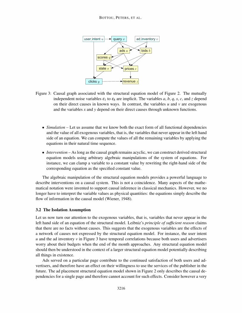
Figure 3: Causal graph associated with the structural equation model of Figure 2. The mutuallyindependent noise variables ε1 to ε8 are implicit. The variables a, b, q, s, c, and z dependon their direct causes in known ways. In contrast, the variables u and v are exogenousand the variables x and y depend on their direct causes through unknown functions.
• Simulation – Let us assume that we know both the exact form of all functional dependenciesand the value of all exogenous variables, that is, the variables that never appear in the left handside of an equation. We can compute the values of all the remaining variables by applying theequations in their natural time sequence.
• Intervention – As long as the causal graph remains acyclic, we can construct derived structuralequation models using arbitrary algebraic manipulations of the system of equations. Forinstance, we can clamp a variable to a constant value by rewriting the right-hand side of thecorresponding equation as the specified constant value.
The algebraic manipulation of the structural equation models provides a powerful language todescribe interventions on a causal system. This is not a coincidence. Many aspects of the mathe-matical notation were invented to support causal inference in classical mechanics. However, we nolonger have to interpret the variable values as physical quantities: the equations simply describe theflow of information in the causal model (Wiener, 1948).
3.2 The Isolation Assumption
Let us now turn our attention to the exogenous variables, that is, variables that never appear in theleft hand side of an equation of the structural model. Leibniz’s principle of sufficient reason claimsthat there are no facts without causes. This suggests that the exogenous variables are the effects ofa network of causes not expressed by the structural equation model. For instance, the user intentu and the ad inventory v in Figure 3 have temporal correlations because both users and advertisersworry about their budgets when the end of the month approaches. Any structural equation modelshould then be understood in the context of a larger structural equation model potentially describingall things in existence.
Ads served on a particular page contribute to the continued satisfaction of both users and ad-vertisers, and therefore have an effect on their willingness to use the services of the publisher in thefuture. The ad placement structural equation model shown in Figure 2 only describes the causal de-pendencies for a single page and therefore cannot account for such effects. Consider however a very
3216
COUNTERFACTUAL REASONING AND LEARNING SYSTEMS
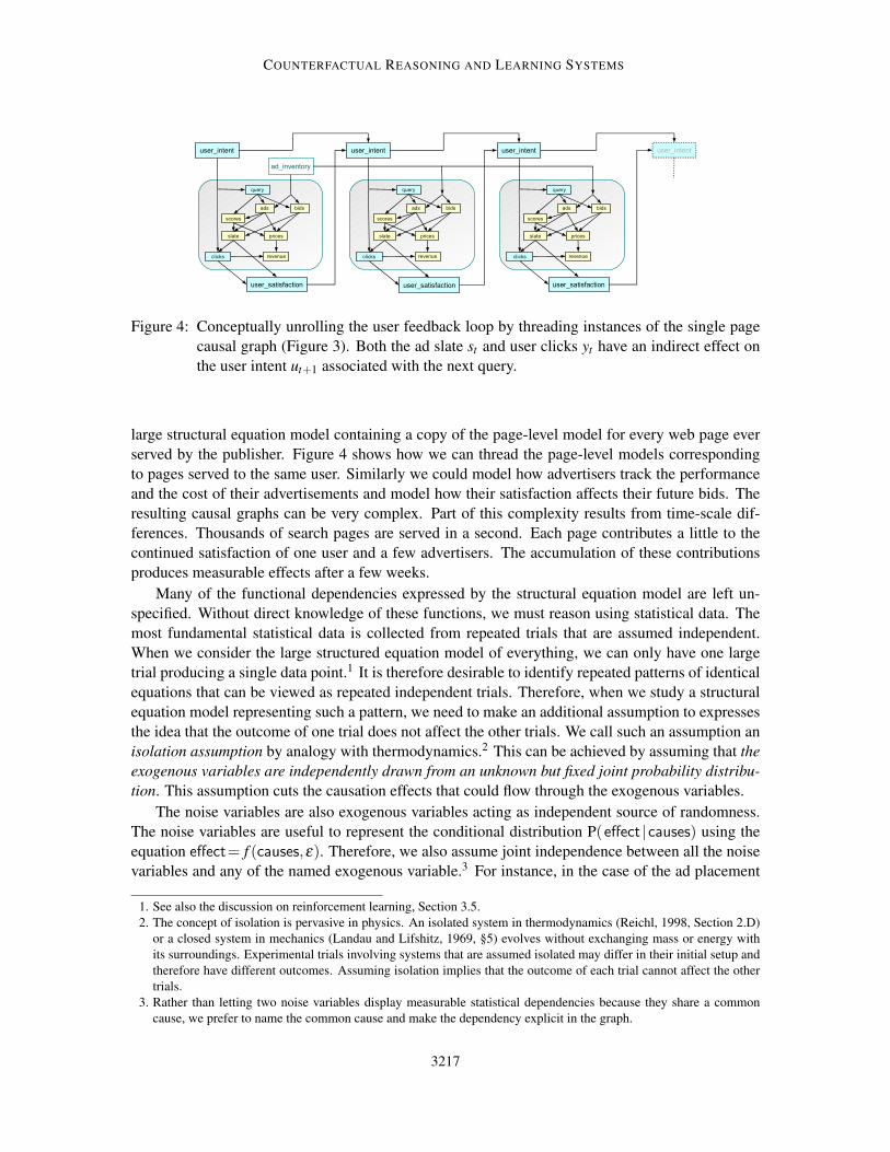
Figure 4: Conceptually unrolling the user feedback loop by threading instances of the single pagecausal graph (Figure 3). Both the ad slate st and user clicks yt have an indirect effect onthe user intent ut+1 associated with the next query.
large structural equation model containing a copy of the page-level model for every web page everserved by the publisher. Figure 4 shows how we can thread the page-level models correspondingto pages served to the same user. Similarly we could model how advertisers track the performanceand the cost of their advertisements and model how their satisfaction affects their future bids. Theresulting causal graphs can be very complex. Part of this complexity results from time-scale dif-ferences. Thousands of search pages are served in a second. Each page contributes a little to thecontinued satisfaction of one user and a few advertisers. The accumulation of these contributionsproduces measurable effects after a few weeks.
Many of the functional dependencies expressed by the structural equation model are left un-specified. Without direct knowledge of these functions, we must reason using statistical data. Themost fundamental statistical data is collected from repeated trials that are assumed independent.When we consider the large structured equation model of everything, we can only have one largetrial producing a single data point.1 It is therefore desirable to identify repeated patterns of identicalequations that can be viewed as repeated independent trials. Therefore, when we study a structuralequation model representing such a pattern, we need to make an additional assumption to expressesthe idea that the outcome of one trial does not affect the other trials. We call such an assumption anisolation assumption by analogy with thermodynamics.2 This can be achieved by assuming that theexogenous variables are independently drawn from an unknown but fixed joint probability distribu-tion. This assumption cuts the causation effects that could flow through the exogenous variables.
The noise variables are also exogenous variables acting as independent source of randomness.The noise variables are useful to represent the conditional distribution P(effect |causes) using theequation effect= f (causes,ε). Therefore, we also assume joint independence between all the noisevariables and any of the named exogenous variable.3 For instance, in the case of the ad placement
1. See also the discussion on reinforcement learning, Section 3.5.2. The concept of isolation is pervasive in physics. An isolated system in thermodynamics (Reichl, 1998, Section 2.D)
or a closed system in mechanics (Landau and Lifshitz, 1969, §5) evolves without exchanging mass or energy withits surroundings. Experimental trials involving systems that are assumed isolated may differ in their initial setup andtherefore have different outcomes. Assuming isolation implies that the outcome of each trial cannot affect the othertrials.
3. Rather than letting two noise variables display measurable statistical dependencies because they share a commoncause, we prefer to name the common cause and make the dependency explicit in the graph.
3217

BOTTOU, PETERS, ET AL.
P(
u,v,x,a,bq,s,c,y,z
)=
P(u,v) Exogenous vars.× P(x |u) Query.× P(a |x,v) Eligible ads.× P(b |x,v) Bids.× P(q |x,a) Scores.× P(s |a,q,b) Ad slate.× P(c |a,q,b) Prices.× P(y |s,u) Clicks.× P(z |y,c) Revenue.
Figure 5: Markov factorization of the structural equation model of Figure 2.
Figure 6: Bayesian network associated with the Markov factorization shown in Figure 5.
model shown in Figure 2, we assume that the joint distribution of the exogenous variables factorizesas
P(u,v,ε1, . . . ,ε8) = P(u,v)P(ε1) . . .P(ε8) .
Since an isolation assumption is only true up to a point, it should be expressed clearly and remainunder constant scrutiny. We must therefore measure additional performance metrics that reveal howthe isolation assumption holds. For instance, the ad placement structural equation model and thecorresponding causal graph (figures 2 and 3) do not take user feedback or advertiser feedback intoaccount. Measuring the revenue is not enough because we could easily generate revenue at theexpense of the satisfaction of the users and advertisers. When we evaluate interventions undersuch an isolation assumption, we also need to measure a battery of additional quantities that act asproxies for the user and advertiser satisfaction. Noteworthy examples include ad relevance estimatedby human judges, and advertiser surplus estimated from the auctions (Varian, 2009).
3.3 Markov Factorization
Conceptually, we can draw a sample of the exogenous variables using the distribution specifiedby the isolation assumption, and we can then generate values for all the remaining variables bysimulating the structural equation model.
3218

COUNTERFACTUAL REASONING AND LEARNING SYSTEMS
This process defines a generative probabilistic model representing the joint distribution of allvariables in the structural equation model. The distribution readily factorizes as the product of thejoint probability of the named exogenous variables, and, for each equation in the structural equationmodel, the conditional probability of the effect given its direct causes (Spirtes et al., 1993; Pearl,2000). As illustrated by figures 5 and 6, this Markov factorization connects the structural equa-tion model that describes causation, and the Bayesian network that describes the joint probabilitydistribution followed by the variables under the isolation assumption.4
Structural equation models and Bayesian networks appear so intimately connected that it couldbe easy to forget the differences. The structural equation model is an algebraic object. As longas the causal graph remains acyclic, algebraic manipulations are interpreted as interventions on thecausal system. The Bayesian network is a generative statistical model representing a class of jointprobability distributions, and, as such, does not support algebraic manipulations. However, thesymbolic representation of its Markov factorization is an algebraic object, essentially equivalent tothe structural equation model.
3.4 Identification, Transportation, and Transfer Learning
Consider a causal system represented by a structural equation model with some unknown functionaldependencies. Subject to the isolation assumption, data collected during the operation of this systemfollows the distribution described by the corresponding Markov factorization. Let us first assumethat this data is sufficient to identify the joint distribution of the subset of variables we can observe.We can intervene on the system by clamping the value of some variables. This amounts to replacingthe right-hand side of the corresponding structural equations by constants. The joint distribution ofthe variables is then described by a new Markov factorization that shares many factors with the orig-inal Markov factorization. Which conditional probabilities associated with this new distribution canwe express using only conditional probabilities identified during the observation of the original sys-tem? This is called the identifiability problem. More generally, we can consider arbitrarily complexmanipulations of the structural equation model, and we can perform multiple experiments involv-ing different manipulations of the causal system. Which conditional probabilities pertaining to oneexperiment can be expressed using only conditional probabilities identified during the observationof other experiments? This is called the transportability problem.
Pearl’s do-calculus completely solves the identifiability problem and provides useful tools toaddress many instances of the transportability problem (see Pearl, 2012). Assuming that we knowthe conditional probability distributions involving observed variables in the original structural equa-tion model, do-calculus allows us to derive conditional distributions pertaining to the manipulatedstructural equation model.
Unfortunately, we must further distinguish the conditional probabilities that we know (becausewe designed them) from those that we estimate from empirical data. This distinction is importantbecause estimating the distribution of continuous or high cardinality variables is notoriously dif-ficult. Furthermore, do-calculus often combines the estimated probabilities in ways that amplifyestimation errors. This happens when the manipulated structural equation model exercises the vari-ables in ways that were rarely observed in the data collected from the original structural equationmodel.
4. Bayesian networks are directed graphs representing the Markov factorization of a joint probability distribution: thearrows no longer have a causal interpretation.
3219

BOTTOU, PETERS, ET AL.
Therefore we prefer to use much simpler causal inference techniques (see sections 4.1 and 4.2).Although these techniques do not have the completeness properties of do-calculus, they combineestimation and transportation in a manner that facilitates the derivation of useful confidence inter-vals.
3.5 Special Cases
Three special cases of causal models are particularly relevant to this work.
• In the multi-armed bandit (Robbins, 1952), a user-defined policy function π determines thedistribution of action a ∈ 1 . . .K, and an unknown reward function r determines the distri-bution of the outcome y given the action a (Figure 7). In order to maximize the accumulatedrewards, the player must construct policies π that balance the exploration of the action spacewith the exploitation of the best action identified so far (Auer et al., 2002; Audibert et al.,2007; Seldin et al., 2012).
• The contextual bandit problem (Langford and Zhang, 2008) significantly increases the com-plexity of multi-armed bandits by adding one exogenous variable x to the policy function π
and the reward functions r (Figure 8).
• Both multi-armed bandit and contextual bandit are special case of reinforcement learning(Sutton and Barto, 1998). In essence, a Markov decision process is a sequence of contextualbandits where the context is no longer an exogenous variable but a state variable that dependson the previous states and actions (Figure 9). Note that the policy function π , the rewardfunction r, and the transition function s are independent of time. All the time dependenciesare expressed using the states st .
These special cases have increasing generality. Many simple structural equation models can bereduced to a contextual bandit problem using appropriate definitions of the context x, the action aand the outcome y. For instance, assuming that the prices c are discrete, the ad placement struc-tural equation model shown in Figure 2 reduces to a contextual bandit problem with context (u,v),actions (s,c) and reward z. Similarly, given a sufficiently intricate definition of the state variablesst , all structural equation models with discrete variables can be reduced to a reinforcement learningproblem. Such reductions lose the fine structure of the causal graph. We show in Section 5 how thisfine structure can in fact be leveraged to obtain more information from the same experiments.
Modern reinforcement learning algorithms (see Sutton and Barto, 1998) leverage the assumptionthat the policy function, the reward function, the transition function, and the distributions of thecorresponding noise variables, are independent from time. This invariance property provides greatbenefits when the observed sequences of actions and rewards are long in comparison with the sizeof the state space. Only Section 7 in this contribution presents methods that take advantage of suchan invariance. The general question of leveraging arbitrary functional invariances in causal graphsis left for future work.
4. Counterfactual Analysis
We now return to the problem of formulating and answering questions about the value of proposedchanges of a learning system. Assume for instance that we consider replacing the score computation
3220
COUNTERFACTUAL REASONING AND LEARNING SYSTEMS
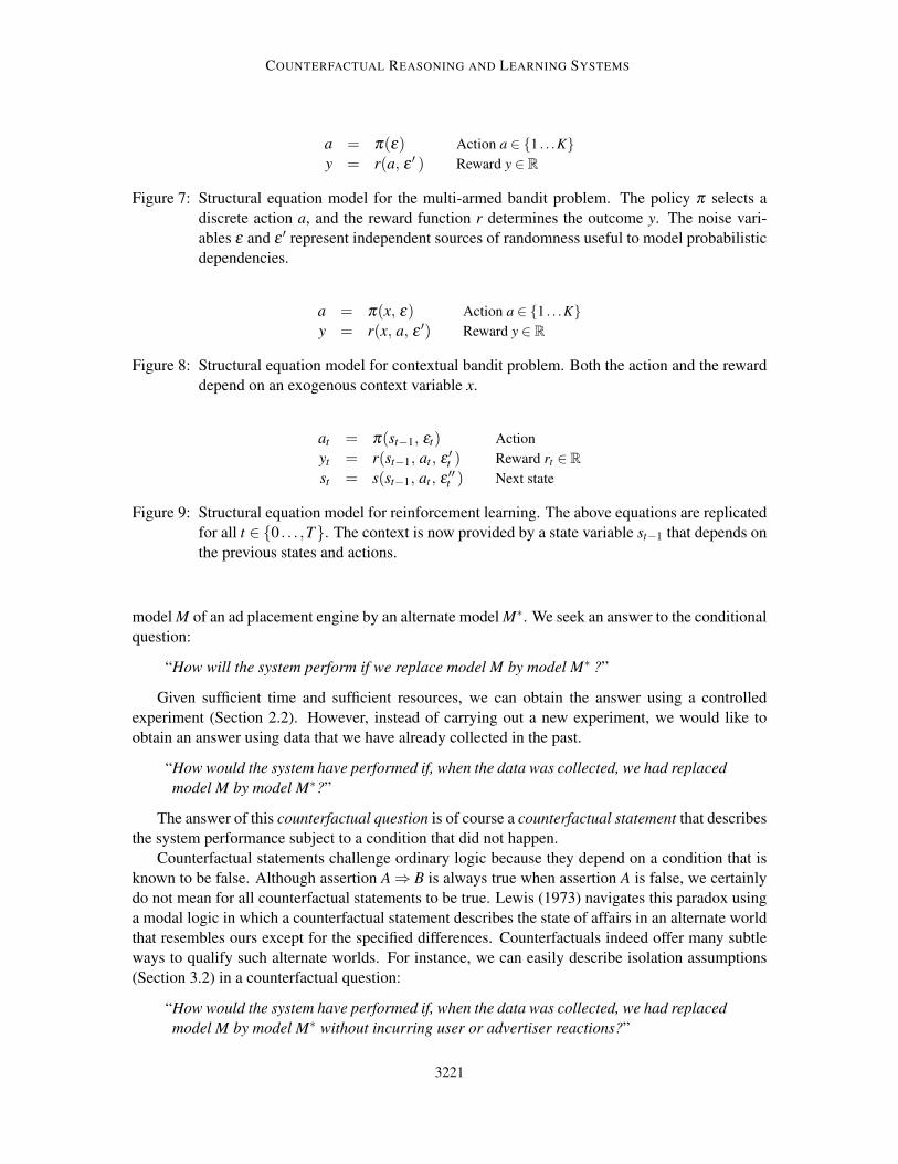
a = π(ε) Action a ∈ 1 . . .Ky = r(a, ε ′ ) Reward y ∈ R
Figure 7: Structural equation model for the multi-armed bandit problem. The policy π selects adiscrete action a, and the reward function r determines the outcome y. The noise vari-ables ε and ε ′ represent independent sources of randomness useful to model probabilisticdependencies.
a = π(x, ε) Action a ∈ 1 . . .Ky = r(x, a, ε ′) Reward y ∈ R
Figure 8: Structural equation model for contextual bandit problem. Both the action and the rewarddepend on an exogenous context variable x.
at = π(st−1, εt) Actionyt = r(st−1, at , ε ′t ) Reward rt ∈ Rst = s(st−1, at , ε ′′t ) Next state
Figure 9: Structural equation model for reinforcement learning. The above equations are replicatedfor all t ∈ 0 . . . ,T. The context is now provided by a state variable st−1 that depends onthe previous states and actions.
model M of an ad placement engine by an alternate model M∗. We seek an answer to the conditionalquestion:
“How will the system perform if we replace model M by model M∗ ?”
Given sufficient time and sufficient resources, we can obtain the answer using a controlledexperiment (Section 2.2). However, instead of carrying out a new experiment, we would like toobtain an answer using data that we have already collected in the past.
“How would the system have performed if, when the data was collected, we had replacedmodel M by model M∗?”
The answer of this counterfactual question is of course a counterfactual statement that describesthe system performance subject to a condition that did not happen.
Counterfactual statements challenge ordinary logic because they depend on a condition that isknown to be false. Although assertion A⇒ B is always true when assertion A is false, we certainlydo not mean for all counterfactual statements to be true. Lewis (1973) navigates this paradox usinga modal logic in which a counterfactual statement describes the state of affairs in an alternate worldthat resembles ours except for the specified differences. Counterfactuals indeed offer many subtleways to qualify such alternate worlds. For instance, we can easily describe isolation assumptions(Section 3.2) in a counterfactual question:
“How would the system have performed if, when the data was collected, we had replacedmodel M by model M∗ without incurring user or advertiser reactions?”
3221

BOTTOU, PETERS, ET AL.
Figure 10: Causal graph for an image recognition system. We can estimate counterfactuals byreplaying data collected in the past.
Figure 11: Causal graph for a randomized experiment. We can estimate certain counterfactuals byreweighting data collected in the past.
The fact that we could not have changed the model without incurring the user and advertiser reac-tions does not matter any more than the fact that we did not replace model M by model M∗ in thefirst place. This does not prevent us from using counterfactual statements to reason about causesand effects. Counterfactual questions and statements provide a natural framework to express andshare our conclusions.
The remaining text in this section explains how we can answer certain counterfactual questionsusing data collected in the past. More precisely, we seek to estimate performance metrics that canbe expressed as expectations with respect to the distribution that would have been observed if thecounterfactual conditions had been in force.5
4.1 Replaying Empirical Data
Figure 10 shows the causal graph associated with a simple image recognition system. The classifiertakes an image x and produces a prospective class label y. The loss measures the penalty associatedwith recognizing class y while the true class is y.
To estimate the expected error of such a classifier, we collect a representative data set composedof labelled images, run the classifier on each image, and average the resulting losses. In other words,we replay the data set to estimate what (counterfactual) performance would have been observed ifwe had used a different classifier. We can then select in retrospect the classifier that would haveworked the best and hope that it will keep working well. This is the counterfactual viewpoint onempirical risk minimization (Vapnik, 1982).
Replaying the data set works because both the alternate classifier and the loss function areknown. More generally, to estimate a counterfactual by replaying a data set, we need to know allthe functional dependencies associated with all causal paths connecting the intervention point to themeasurement point. This is obviously not always the case.
5. Although counterfactual expectations can be viewed as expectations of unit-level counterfactuals (Pearl, 2009, Def-inition 4), they elude the semantic subtleties of unit-level counterfactuals and can be measured with randomizedexperiments (see Section 4.2.)
3222

COUNTERFACTUAL REASONING AND LEARNING SYSTEMS
4.2 Reweighting Randomized Trials
Figure 11 illustrates the randomized experiment suggested in Section 2.3. The patients are randomlysplit into two equally sized groups receiving respectively treatments A and B. The overall successrate for this experiment is therefore Y = (YA+YB)/2 where YA and YB are the success rates observedfor each group. We would like to estimate which (counterfactual) overall success rate Y ∗ would havebeen observed if we had selected treatment A with probability p and treatment B with probability1− p.
Since we do not know how the outcome depends on the treatment and the patient condition,we cannot compute which outcome y∗ would have been obtained if we had treated patient x with adifferent treatment u∗. Therefore we cannot answer this question by replaying the data as we did inSection 4.1.
However, observing different success rates YA and YB for the treatment groups reveals an empir-ical correlation between the treatment u and the outcome y. Since the only cause of the treatment uis an independent roll of the dices, this correlation cannot result from any known or unknown con-founding common cause.6 Having eliminated this possibility, we can reweight the observed out-comes and compute the estimate Y ∗ ≈ pYA +(1− p)YB .
4.3 Markov Factor Replacement
The reweighting approach can in fact be applied under much less stringent conditions. Let us returnto the ad placement problem to illustrate this point.
The average number of ad clicks per page is often called click yield. Increasing the click yieldusually benefits both the advertiser and the publisher, whereas increasing the revenue per pageoften benefits the publisher at the expense of the advertiser. Click yield is therefore a very usefulmetric when we reason with an isolation assumption that ignores the advertiser reactions to pricingchanges.
Let ω be a shorthand for all variables appearing in the Markov factorization of the ad placementstructural equation model,
P(ω) = P(u,v)P(x |u)P(a |x,v)P(b |x,v)P(q |x,a)× P(s |a,q,b)P(c |a,q,b)P(y |s,u)P(z |y,c) . (2)
Variable y was defined in Section 3.1 as the set of user clicks. In the rest of the document, weslightly abuse this notation by using the same letter y to represent the number of clicks. We alsowrite the expectation Y = Eω∼P(ω)[y] using the integral notation
Y =∫
ω
y P(ω) .
We would like to estimate what the expected click yield Y ∗ would have been if we had useda different scoring function (Figure 12). This intervention amounts to replacing the actual factorP(q |x,a) by a counterfactual factor P∗(q |x,a) in the Markov factorization.
P∗(ω) = P(u,v)P(x |u)P(a |x,v)P(b |x,v)P∗(q |x,a)× P(s |a,q,b)P(c |a,q,b)P(y |s,u)P(z |x,c) . (3)
6. See also the discussion of Reichenbach’s common cause principle and of its limitations in Spirtes et al. (1993) andSpirtes and Scheines (2004).
3223
BOTTOU, PETERS, ET AL.
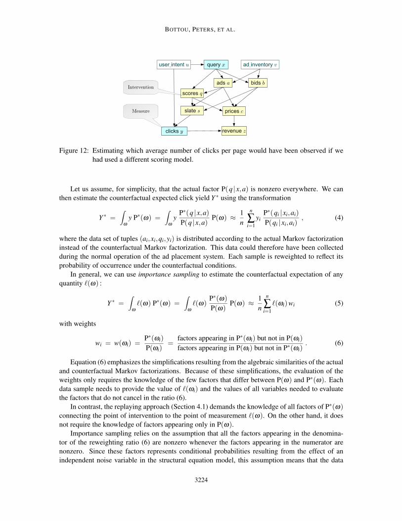
Figure 12: Estimating which average number of clicks per page would have been observed if wehad used a different scoring model.
Let us assume, for simplicity, that the actual factor P(q |x,a) is nonzero everywhere. We canthen estimate the counterfactual expected click yield Y ∗ using the transformation
Y ∗ =∫
ω
y P∗(ω) =∫
ω
yP∗(q |x,a)P(q |x,a)
P(ω) ≈ 1n
n
∑i=1
yiP∗(qi |xi,ai)
P(qi |xi,ai), (4)
where the data set of tuples (ai,xi,qi,yi) is distributed according to the actual Markov factorizationinstead of the counterfactual Markov factorization. This data could therefore have been collectedduring the normal operation of the ad placement system. Each sample is reweighted to reflect itsprobability of occurrence under the counterfactual conditions.
In general, we can use importance sampling to estimate the counterfactual expectation of anyquantity `(ω) :
Y ∗ =∫
ω
`(ω) P∗(ω) =∫
ω
`(ω)P∗(ω)
P(ω)P(ω) ≈ 1
n
n
∑i=1
`(ωi)wi (5)
with weights
wi = w(ωi) =P∗(ωi)
P(ωi)=
factors appearing in P∗(ωi) but not in P(ωi)
factors appearing in P(ωi) but not in P∗(ωi). (6)
Equation (6) emphasizes the simplifications resulting from the algebraic similarities of the actualand counterfactual Markov factorizations. Because of these simplifications, the evaluation of theweights only requires the knowledge of the few factors that differ between P(ω) and P∗(ω). Eachdata sample needs to provide the value of `(ωi) and the values of all variables needed to evaluatethe factors that do not cancel in the ratio (6).
In contrast, the replaying approach (Section 4.1) demands the knowledge of all factors of P∗(ω)connecting the point of intervention to the point of measurement `(ω). On the other hand, it doesnot require the knowledge of factors appearing only in P(ω).
Importance sampling relies on the assumption that all the factors appearing in the denomina-tor of the reweighting ratio (6) are nonzero whenever the factors appearing in the numerator arenonzero. Since these factors represents conditional probabilities resulting from the effect of anindependent noise variable in the structural equation model, this assumption means that the data
3224

COUNTERFACTUAL REASONING AND LEARNING SYSTEMS
must be collected with an experiment involving active randomization. We must therefore designcost-effective randomized experiments that yield enough information to estimate many interestingcounterfactual expectations with sufficient accuracy. This problem cannot be solved without an-swering the confidence interval question: given data collected with a certain level of randomization,with which accuracy can we estimate a given counterfactual expectation?
4.4 Confidence Intervals
At first sight, we can invoke the law of large numbers and write
Y ∗ =∫
ω
`(ω)w(ω) P(ω) ≈ 1n
n
∑i=1
`(ωi)wi . (7)
For sufficiently large n, the central limit theorem provides confidence intervals whose width growswith the standard deviation of the product `(ω)w(ω).
Unfortunately, when P(ω) is small, the reweighting ratio w(ω) takes large values with lowprobability. This heavy tailed distribution has annoying consequences because the variance of theintegrand could be very high or infinite. When the variance is infinite, the central limit theoremdoes not hold. When the variance is merely very large, the central limit convergence might occurtoo slowly to justify such confidence intervals. Importance sampling works best when the actualdistribution and the counterfactual distribution overlap.
When the counterfactual distribution has significant mass in domains where the actual distribu-tion is small, the few samples available in these domains receive very high weights. Their noisycontribution dominates the reweighted estimate (7). We can obtain better confidence intervals byeliminating these few samples drawn in poorly explored domains. The resulting bias can be boundedusing prior knowledge, for instance with an assumption about the range of values taken by `(ω),
∀ω `(ω) ∈ [0, M] . (8)
Let us choose the maximum weight value R deemed acceptable for the weights. We have ob-tained very consistent results in practice with R equal to the fifth largest reweighting ratio observedon the empirical data.7 We can then rely on clipped weights to eliminate the contribution of thepoorly explored domains,
w(ω) =
w(ω) if P∗(ω)< R P(ω)0 otherwise.
The condition P∗(ω)< RP(ω) ensures that the ratio has a nonzero denominator P(ω) and is smallerthan R. Let ΩR be the set of all values of ω associated with acceptable ratios:
ΩR = ω : P∗(ω)< R P(ω) .
We can decompose Y ∗ in two terms:
Y ∗ =∫
ω∈ΩR
`(ω)P∗(ω) +∫
ω∈Ω\ΩR
`(ω)P∗(ω) = Y ∗+(Y ∗− Y ∗) . (9)
7. This is in fact a slight abuse because the theory calls for choosing R before seeing the data.
3225

BOTTOU, PETERS, ET AL.
The first term of this decomposition is the clipped expectation Y ∗. Estimating the clipped expec-tation Y ∗ is much easier than estimating Y ∗ from (7) because the clipped weights w(ω) are boundedby R.
Y ∗ =∫
ω∈ΩR
`(ω)P∗(ω) =∫
ω
`(ω) w(ω) P(ω) ≈ Y ∗ =1n
n
∑i=1
`(ωi) w(ωi) . (10)
The second term of Equation (9) can be bounded by leveraging assumption (8). The resultingbound can then be conveniently estimated using only the clipped weights.
Y ∗− Y ∗ =∫
ω∈Ω\ΩR
`(ω)P∗(ω) ∈[
0, M P∗(Ω\ΩR)]=[
0, M (1−W ∗)]
with
W ∗ = P∗(ΩR) =∫
ω∈ΩR
P∗(ω) =∫
ω
w(ω)P(ω) ≈ W ∗ =1n
n
∑i=1
w(ωi) . (11)
Since the clipped weights are bounded, the estimation errors associated with (10) and (11) arewell characterized using either the central limit theorem or using empirical Bernstein bounds (seeappendix B for details). Therefore we can derive an outer confidence interval of the form
P
Y ∗− εR ≤ Y ∗ ≤ Y ∗+ εR
≥ 1−δ (12)
and an inner confidence interval of the form
P
Y ∗ ≤ Y ∗ ≤ Y ∗+M(1−W ∗+ξR)≥ 1−δ . (13)
The names inner and outer are in fact related to our preferred way to visualize these intervals (e.g.,Figure 13). Since the bounds on Y ∗− Y ∗ can be written as
Y ∗ ≤ Y ∗ ≤ Y ∗+M (1−W ∗) , (14)
we can derive our final confidence interval,
P
Y ∗− εR ≤ Y ∗ ≤ Y ∗+M(1−W ∗+ξR)+ εR
≥ 1−2δ . (15)
In conclusion, replacing the unbiased importance sampling estimator (7) by the clipped impor-tance sampling estimator (10) with a suitable choice of R leads to improved confidence intervals.Furthermore, since the derivation of these confidence intervals does not rely on the assumption thatP(ω) is nonzero everywhere, the clipped importance sampling estimator remains valid when the dis-tribution P(ω) has a limited support. This relaxes the main restriction associated with importancesampling.
4.5 Interpreting the Confidence Intervals
The estimation of the counterfactual expectation Y ∗ can be inaccurate because the sample size is in-sufficient or because the sampling distribution P(ω) does not sufficiently explore the counterfactualconditions of interest.
By construction, the clipped expectation Y ∗ ignores the domains poorly explored by the sam-pling distribution P(ω). The difference Y ∗− Y ∗ then reflects the inaccuracy resulting from a lackof exploration. Therefore, assuming that the bound R has been chosen competently, the relativesizes of the outer and inner confidence intervals provide precious cues to determine whether wecan continue collecting data using the same experimental setup or should adjust the data collectionexperiment in order to obtain a better coverage.
3226

COUNTERFACTUAL REASONING AND LEARNING SYSTEMS
• The inner confidence interval (13) witnesses the uncertainty associated with the domain GR
insufficiently explored by the actual distribution. A large inner confidence interval suggeststhat the most practical way to improve the estimate is to adjust the data collection experimentin order to obtain a better coverage of the counterfactual conditions of interest.
• The outer confidence interval (12) represents the uncertainty that results from the limitedsample size. A large outer confidence interval indicates that the sample is too small. Toimprove the result, we simply need to continue collecting data using the same experimentalsetup.
4.6 Experimenting with Mainline Reserves
We return to the ad placement problem to illustrate the reweighting approach and the interpretationof the confidence intervals. Manipulating the reserves Rp(x) associated with the mainline positions(Figure 1) controls which ads are prominently displayed in the mainline or displaced into the sidebar.
We seek in this section to answer counterfactual questions of the form:
“How would the ad placement system have performed if we had scaled the mainlinereserves by a constant factor ρ , without incurring user or advertiser reactions?”
Randomization was introduced using a modified version of the ad placement engine. Beforedetermining the ad layout (see Section 2.1), a random number ε is drawn according to the standardnormal distribution N (0,1), and all the mainline reserves are multiplied by m = ρ e−σ2/2+σε . Suchmultipliers follow a log-normal distribution8 whose mean is ρ and whose width is controlled byσ . This effectively provides a parametrization of the conditional score distribution P(q |x,a) (seeFigure 5.)
The Bing search platform offers many ways to select traffic for controlled experiments (Sec-tion 2.2). In order to match our isolation assumption, individual page views were randomly as-signed to traffic buckets without regard to the user identity. The main treatment bucket was pro-cessed with mainline reserves randomized by a multiplier drawn as explained above with ρ =1 andσ = 0.3. With these parameters, the mean multiplier is exactly 1, and 95% of the multipliers arein range [0.52,1.74]. Samples describing 22 million search result pages were collected during fiveconsecutive weeks.
We then use this data to estimate what would have been measured if the mainline reserve mul-tipliers had been drawn according to a distribution determined by parameters ρ∗ and σ∗. This isachieved by reweighting each sample ωi with
wi =P∗(qi |xi,ai)
P(qi |xi,ai)=
p(mi ; ρ∗, σ∗)
p(mi ; ρ, σ),
where mi is the multiplier drawn for this sample during the data collection experiment, and p(t ; ρ,σ)is the density of the log-normal multiplier distribution.
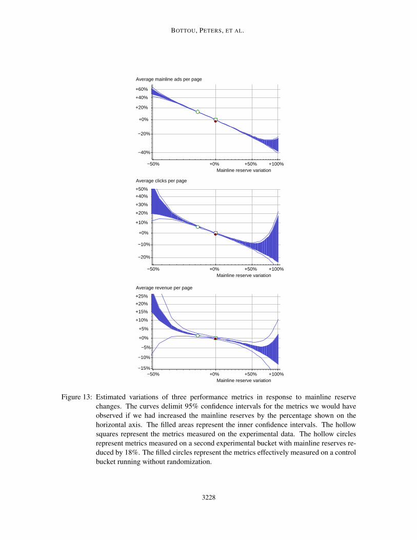
Figure 13 reports results obtained by varying ρ∗ while keeping σ∗=σ . This amounts to esti-mating what would have been measured if all mainline reserves had been multiplied by ρ∗ whilekeeping the same randomization. The curves bound 95% confidence intervals on the variations ofthe average number of mainline ads displayed per page, the average number of ad clicks per page,
8. More precisely, lnN (µ,σ2) with µ = σ2/2+ logρ .
3227
BOTTOU, PETERS, ET AL.
−40%
−20%
+0%
+20%
+40%
+60%
−50% +0% +50% +100%Mainline reserve variation
Average mainline ads per page
−20%
−10%
+0%
+10%
+20%
+30%
+40%
+50%
−50% +0% +50% +100%Mainline reserve variation
Average clicks per page
−15%
−10%
−5%
+0%
+5%
+10%
+15%
+20%
+25%
−50% +0% +50% +100%Mainline reserve variation
Average revenue per page
Figure 13: Estimated variations of three performance metrics in response to mainline reservechanges. The curves delimit 95% confidence intervals for the metrics we would haveobserved if we had increased the mainline reserves by the percentage shown on thehorizontal axis. The filled areas represent the inner confidence intervals. The hollowsquares represent the metrics measured on the experimental data. The hollow circlesrepresent metrics measured on a second experimental bucket with mainline reserves re-duced by 18%. The filled circles represent the metrics effectively measured on a controlbucket running without randomization.
3228

COUNTERFACTUAL REASONING AND LEARNING SYSTEMS
and the average revenue per page, as functions of ρ∗. The inner confidence intervals, representedby the filled areas, grow sharply when ρ∗ leaves the range explored during the data collection ex-periment. The average revenue per page has more variance because a few very competitive queriescommand high prices.
In order to validate the accuracy of these counterfactual estimates, a second traffic bucket ofequal size was configured with mainline reserves reduced by about 18%. The hollow circles inFigure 13 represent the metrics effectively measured on this bucket during the same time period.The effective measurements and the counterfactual estimates match with high accuracy.
Finally, in order to measure the cost of the randomization, we also ran the unmodified ad place-ment system on a control bucket. The brown filled circles in Figure 13 represent the metrics effec-tively measured on the control bucket during the same time period. The randomization caused asmall but statistically significant increase of the number of mainline ads per page. The click yieldand average revenue differences are not significant.
This experiment shows that we can obtain accurate counterfactual estimates with affordablerandomization strategies. However, this nice conclusion does not capture the true practical value ofthe counterfactual estimation approach.
4.7 More on Mainline Reserves
The main benefit of the counterfactual estimation approach is the ability to use the same data toanswer a broad range of counterfactual questions. Here are a few examples of counterfactual ques-tions that can be answered using data collected using the simple mainline reserve randomizationscheme described in the previous section:
• Different variances – Instead of estimating what would have been measured if we had in-creased the mainline reserves without changing the randomization variance, that is, lettingσ∗ = σ , we can use the same data to estimate what would have been measured if we had alsochanged σ . This provides the means to determine which level of randomization we can affordin future experiments.
• Pointwise estimates – We often want to estimate what would have been measured if we hadset the mainline reserves to a specific value without randomization. Although computingestimates for small values of σ often works well enough, very small values lead to largeconfidence intervals.
Let Yν(ρ) represent the expectation we would have observed if the multipliers m had mean ρ
and variance ν . We have then Yν(ρ) =Em[E[y|m] ] =Em[Y0(m)]. Assuming that the pointwisevalue Y0 is smooth enough for a second order development,
Yν(ρ) ≈ Em[
Y0(ρ)+(m−ρ)Y ′0(ρ)+(m−ρ)2Y ′′0 (ρ)/2]= Y0(ρ)+νY ′′0 (ρ)/2 .
Although the reweighting method cannot estimate the point-wise value Y0(ρ) directly, we canuse the reweighting method to estimate both Yν(ρ) and Y2ν(ρ) with acceptable confidenceintervals and write Y0(ρ)≈ 2Yν(ρ)−Y2ν(ρ) (Goodwin, 2011).
• Query-dependent reserves – Compare for instance the queries “car insurance” and “com-mon cause principle” in a web search engine. Since the advertising potential of a search
3229
BOTTOU, PETERS, ET AL.
varies considerably with the query, it makes sense to investigate various ways to define query-dependent reserves (Charles and Chickering, 2012).
The data collected using the simple mainline reserve randomization can also be used to es-timate what would have been measured if we had increased all the mainline reserves by aquery-dependent multiplier ρ∗(x). This is simply achieved by reweighting each sample ωi
with
wi =P∗(qi |xi,ai)
P(qi |xi,ai)=
p(mi ; ρ∗(xi) , σ)
p(mi ; µ, σ).
Considerably broader ranges of counterfactual questions can be answered when data is collectedusing randomization schemes that explore more dimensions. For instance, in the case of the adplacement problem, we could apply an independent random multiplier for each score instead ofapplying a single random multiplier to the mainline reserves only. However, the more dimensionswe randomize, the more data needs to be collected to effectively explore all these dimensions.Fortunately, as discussed in section 5, the structure of the causal graph reveals many ways to leveragea priori information and improve the confidence intervals.
4.8 Related Work
Importance sampling is widely used to deal with covariate shifts (Shimodaira, 2000; Sugiyama et al.,2007). Since manipulating the causal graph changes the data distribution, such an intervention canbe viewed as a covariate shift amenable to importance sampling. Importance sampling techniqueshave also been proposed without causal interpretation for many of the problems that we view ascausal inference problems. In particular, the work presented in this section is closely related to theMonte-Carlo approach of reinforcement learning (Sutton and Barto, 1998, Chapter 5) and to theoffline evaluation of contextual bandit policies (Li et al., 2010, 2011).
Reinforcement learning research traditionally focuses on control problems with relatively smalldiscrete state spaces and long sequences of observations. This focus reduces the need for char-acterizing exploration with tight confidence intervals. For instance, Sutton and Barto suggest tonormalize the importance sampling estimator by 1/∑i w(ωi) instead of 1/n. This would give erro-neous results when the data collection distribution leaves parts of the state space poorly explored.Contextual bandits are traditionally formulated with a finite set of discrete actions. For instance, Li’s(2011) unbiased policy evaluation assumes that the data collection policy always selects an arbitrarypolicy with probability greater than some small constant. This is not possible when the action spaceis infinite.
Such assumptions on the data collection distribution are often impractical. For instance, certainad placement policies are not worth exploring because they cannot be implemented efficiently orare known to elicit fraudulent behaviors. There are many practical situations in which one is onlyinterested in limited aspects of the ad placement policy involving continuous parameters such asclick prices or reserves. Discretizing such parameters eliminates useful a priori knowledge: forinstance, if we slightly increase a reserve, we can reasonable believe that we are going to showslightly less ads.
Instead of making assumptions on the data collection distribution, we construct a biased estima-tor (10) and bound its bias. We then interpret the inner and outer confidence intervals as resultingfrom a lack of exploration or an insufficient sample size.
3230
COUNTERFACTUAL REASONING AND LEARNING SYSTEMS
Finally, the causal framework allows us to easily formulate counterfactual questions that pertainto the practical ad placement problem and yet differ considerably in complexity and explorationrequirements. We can address specific problems identified by the engineers without incurring therisks associated with a complete redesign of the system. Each of these incremental steps helpsdemonstrating the soundness of the approach.
5. Structure
This section shows how the structure of the causal graph reveals many ways to leverage a prioriknowledge and improve the accuracy of our counterfactual estimates. Displacing the reweightingpoint (Section 5.1) improves the inner confidence interval and therefore reduce the need for explo-ration. Using a prediction function (Section 5.2) essentially improve the outer confidence intervaland therefore reduce the sample size requirements.
5.1 Better Reweighting Variables
Many search result pages come without eligible ads. We then know with certainty that such pageswill have zero mainline ads, receive zero clicks, and generate zero revenue. This is true for therandomly selected value of the reserve, and this would have been true for any other value of thereserve. We can exploit this knowledge by pretending that the reserve was drawn from the coun-terfactual distribution P∗(q |xi,ai) instead of the actual distribution P(q |xi,ai). The ratio w(ωi) istherefore forced to the unity. This does not change the estimate but reduces the size of the innerconfidence interval. The results of Figure 13 were in fact helped by this little optimization.
There are in fact many circumstances in which the observed outcome would have been thesame for other values of the randomized variables. This prior knowledge is in fact encoded inthe structure of the causal graph and can be exploited in a more systematic manner. For instance,we know that users make click decisions without knowing which scores were computed by the adplacement engine, and without knowing the prices charged to advertisers. The ad placement causalgraph encodes this knowledge by showing the clicks y as direct effects of the user intent u and thead slate s. This implies that the exact value of the scores q does not matter to the clicks y as long asthe ad slate s remains the same.
Because the causal graph has this special structure, we can simplify both the actual and counter-factual Markov factorizations (2) (3) without eliminating the variable y whose expectation is sought.Successively eliminating variables z, c, and q gives:
P(u,v,x,a,b,s,y) = P(u,v)P(x |u)P(a |x,v)P(b |x,v)P(s |x,a,b)P(y |s,u) ,P∗(u,v,x,a,b,s,y) = P(u,v)P(x |u)P(a |x,v)P(b |x,v)P∗(s |x,a,b)P(y |s,u) .
The conditional distributions P(s |x,a,b) and P∗(s |x,a,b) did not originally appear in the Markovfactorization. They are defined by marginalization as a consequence of the elimination of the vari-able q representing the scores.
P(s |x,a,b) =∫
qP(s |a,q,b)P(q |x,a) , P∗(s |x,a,b) =
∫q
P(s |a,q,b)P∗(q |x,a) .
3231
BOTTOU, PETERS, ET AL.
−40%
−20%
+0%
+20%
+40%
+60%
−50% +0% +50% +100%Mainline reserve variation
Average mainline ads per page
−20%
−10%
+0%
+10%
+20%
+30%
+40%
+50%
−50% +0% +50% +100%Mainline reserve variation
Average clicks per page
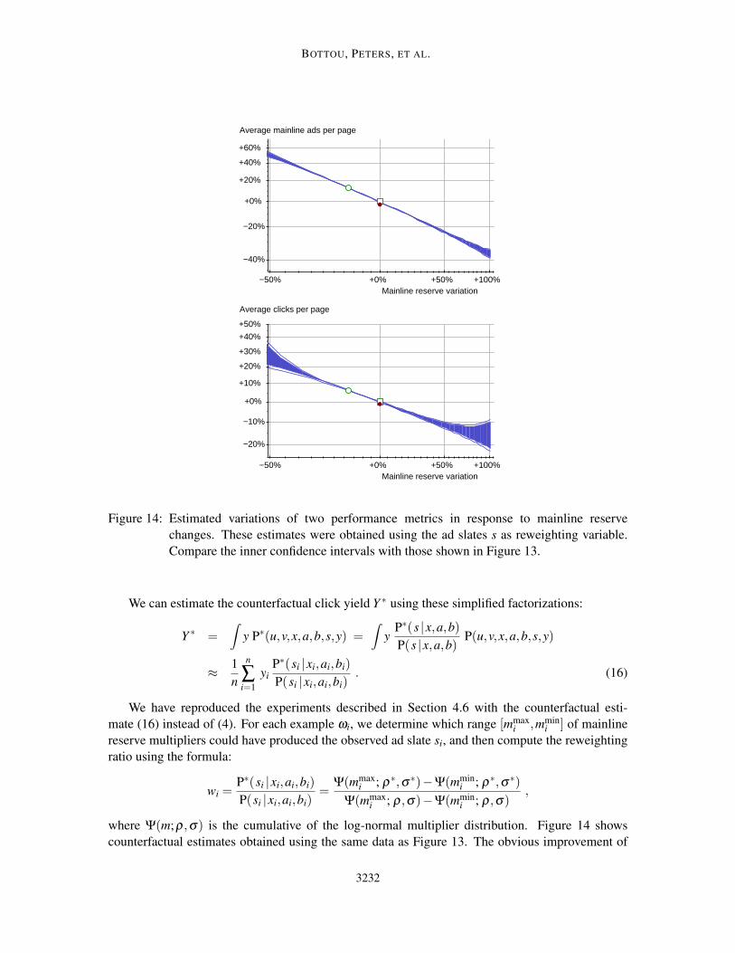
Figure 14: Estimated variations of two performance metrics in response to mainline reservechanges. These estimates were obtained using the ad slates s as reweighting variable.Compare the inner confidence intervals with those shown in Figure 13.
We can estimate the counterfactual click yield Y ∗ using these simplified factorizations:
Y ∗ =∫
y P∗(u,v,x,a,b,s,y) =∫
yP∗(s |x,a,b)P(s |x,a,b)
P(u,v,x,a,b,s,y)
≈ 1n
n
∑i=1
yiP∗(si |xi,ai,bi)
P(si |xi,ai,bi). (16)
We have reproduced the experiments described in Section 4.6 with the counterfactual esti-mate (16) instead of (4). For each example ωi, we determine which range [mmax
i ,mmini ] of mainline
reserve multipliers could have produced the observed ad slate si, and then compute the reweightingratio using the formula:
wi =P∗(si |xi,ai,bi)
P(si |xi,ai,bi)=
Ψ(mmaxi ; ρ∗,σ∗)−Ψ(mmin
i ; ρ∗,σ∗)
Ψ(mmaxi ; ρ,σ)−Ψ(mmin
i ; ρ,σ),
where Ψ(m;ρ,σ) is the cumulative of the log-normal multiplier distribution. Figure 14 showscounterfactual estimates obtained using the same data as Figure 13. The obvious improvement of
3232
COUNTERFACTUAL REASONING AND LEARNING SYSTEMS
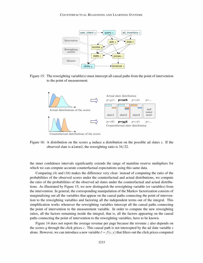
Figure 15: The reweighting variable(s) must intercept all causal paths from the point of interventionto the point of measurement.
Figure 16: A distribution on the scores q induce a distribution on the possible ad slates s. If theobserved slate is slate2, the reweighting ratio is 34/22.
the inner confidence intervals significantly extends the range of mainline reserve multipliers forwhich we can compute accurate counterfactual expectations using this same data.
Comparing (4) and (16) makes the difference very clear: instead of computing the ratio of theprobabilities of the observed scores under the counterfactual and actual distributions, we computethe ratio of the probabilities of the observed ad slates under the counterfactual and actual distribu-tions. As illustrated by Figure 15, we now distinguish the reweighting variable (or variables) fromthe intervention. In general, the corresponding manipulation of the Markov factorization consists ofmarginalizing out all the variables that appear on the causal paths connecting the point of interven-tion to the reweighting variables and factoring all the independent terms out of the integral. Thissimplification works whenever the reweighting variables intercept all the causal paths connectingthe point of intervention to the measurement variable. In order to compute the new reweightingratios, all the factors remaining inside the integral, that is, all the factors appearing on the causalpaths connecting the point of intervention to the reweighting variables, have to be known.
Figure 14 does not report the average revenue per page because the revenue z also depends onthe scores q through the click prices c. This causal path is not intercepted by the ad slate variable salone. However, we can introduce a new variable c= f (c,y) that filters out the click prices computed
3233

BOTTOU, PETERS, ET AL.
for ads that did not receive a click. Markedly improved revenue estimates are then obtained byreweighting according to the joint variable (s, c).
Figure 16 illustrates the same approach applied to the simultaneous randomization of all thescores q using independent log-normal multipliers. The weight w(ωi) is the ratio of the probabilitiesof the observed ad slate si under the counterfactual and actual multiplier distributions. Computingthese probabilities amounts to integrating a multivariate Gaussian distribution (Genz, 1992). Detailswill be provided in a forthcoming publication.
5.2 Variance Reduction with Predictors
Although we do not know exactly how the variable of interest `(ω) depends on the measurable vari-ables and are affected by interventions on the causal graph, we may have strong a priori knowledgeabout this dependency. For instance, if we augment the slate s with an ad that usually receives a lotof clicks, we can expect an increase of the number of clicks.
Let the invariant variables υ be all observed variables that are not direct or indirect effects ofvariables affected by the intervention under consideration. This definition implies that the distri-bution of the invariant variables is not affected by the intervention. Therefore the values υi of theinvariant variables sampled during the actual experiment are also representative of the distributionof the invariant variables under the counterfactual conditions.
We can leverage a priori knowledge to construct a predictor ζ (ω) of the quantity `(ω) whosecounterfactual expectation Y ∗ is sought. We assume that the predictor ζ (ω) depends only on theinvariant variables or on variables that depend on the invariant variables through known functionaldependencies. Given sampled values υi of the invariant variables, we can replay both the originaland manipulated structural equation model as explained in Section 4.1 and obtain samples ζi and ζ ∗ithat respectively follow the actual and counterfactual distributions
Then, regardless of the quality of the predictor,
Y ∗ =∫
ω
`(ω)P∗(ω) =∫
ω
ζ (ω)P∗(ω) +∫
ω
(`(ω)−ζ (ω))P∗(ω)
≈ 1n
n
∑i=1
ζ∗i +
1n
n
∑i=1
(`(ωi)−ζi)w(ωi) . (17)
The first term in this sum represents the counterfactual expectation of the predictor and can be accu-rately estimated by averaging the simulated counterfactual samples ζ ∗i without resorting to poten-tially large importance weights. The second term in this sum represents the counterfactual expecta-tion of the residuals `(ω)−ζ (ω) and must be estimated using importance sampling. Since the mag-nitude of the residuals is hopefully smaller than that of `(ω), the variance of (`(ω)−ζ (ω))w(ω)is reduced and the importance sampling estimator of the second term has improved confidence in-tervals. The more accurate the predictor ζ (ω), the more effective this variance reduction strategy.
This variance reduction technique is in fact identical to the doubly robust contextual bandit eval-uation technique of Dudík et al. (2012). Doubly robust variance reduction has also been extensivelyused for causal inference applied to biostatistics (see Robins et al., 2000; Bang and Robins, 2005).We subjectively find that viewing the predictor as a component of the causal graph (Figure 17) clar-ifies how a well designed predictor can leverage prior knowledge. For instance, in order to estimatethe counterfactual performance of the ad placement system, we can easily use a predictor that runsthe ad auction and simulate the user clicks using a click probability model trained offline.
3234
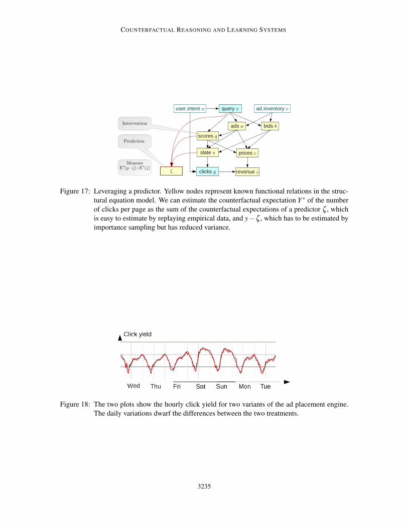
COUNTERFACTUAL REASONING AND LEARNING SYSTEMS
Figure 17: Leveraging a predictor. Yellow nodes represent known functional relations in the struc-tural equation model. We can estimate the counterfactual expectation Y ∗ of the numberof clicks per page as the sum of the counterfactual expectations of a predictor ζ , whichis easy to estimate by replaying empirical data, and y−ζ , which has to be estimated byimportance sampling but has reduced variance.
Figure 18: The two plots show the hourly click yield for two variants of the ad placement engine.The daily variations dwarf the differences between the two treatments.
3235
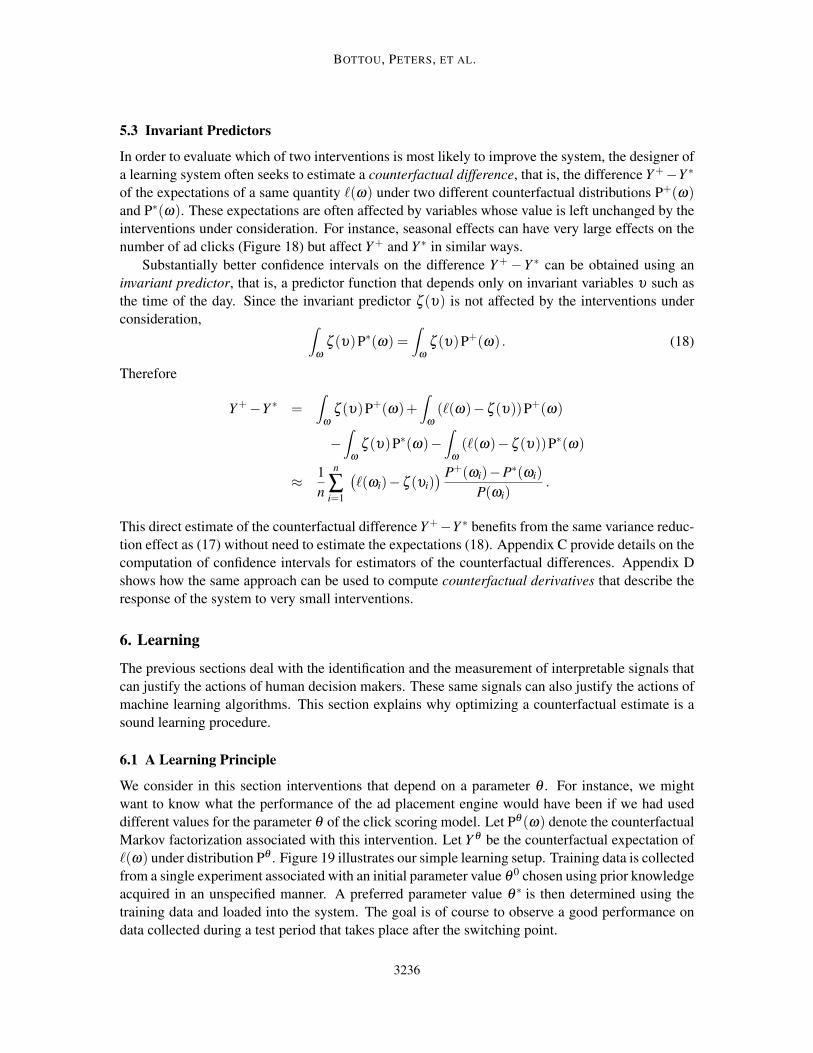
BOTTOU, PETERS, ET AL.
5.3 Invariant Predictors
In order to evaluate which of two interventions is most likely to improve the system, the designer ofa learning system often seeks to estimate a counterfactual difference, that is, the difference Y+−Y ∗
of the expectations of a same quantity `(ω) under two different counterfactual distributions P+(ω)and P∗(ω). These expectations are often affected by variables whose value is left unchanged by theinterventions under consideration. For instance, seasonal effects can have very large effects on thenumber of ad clicks (Figure 18) but affect Y+ and Y ∗ in similar ways.
Substantially better confidence intervals on the difference Y+−Y ∗ can be obtained using aninvariant predictor, that is, a predictor function that depends only on invariant variables υ such asthe time of the day. Since the invariant predictor ζ (υ) is not affected by the interventions underconsideration, ∫
ω
ζ (υ)P∗(ω) =∫
ω
ζ (υ)P+(ω) . (18)
Therefore
Y+−Y ∗ =∫
ω
ζ (υ)P+(ω)+∫
ω
(`(ω)−ζ (υ))P+(ω)
−∫
ω
ζ (υ)P∗(ω)−∫
ω
(`(ω)−ζ (υ))P∗(ω)
≈ 1n
n
∑i=1
(`(ωi)−ζ (υi)
) P+(ωi)−P∗(ωi)
P(ωi).
This direct estimate of the counterfactual difference Y+−Y ∗ benefits from the same variance reduc-tion effect as (17) without need to estimate the expectations (18). Appendix C provide details on thecomputation of confidence intervals for estimators of the counterfactual differences. Appendix Dshows how the same approach can be used to compute counterfactual derivatives that describe theresponse of the system to very small interventions.
6. Learning
The previous sections deal with the identification and the measurement of interpretable signals thatcan justify the actions of human decision makers. These same signals can also justify the actions ofmachine learning algorithms. This section explains why optimizing a counterfactual estimate is asound learning procedure.
6.1 A Learning Principle
We consider in this section interventions that depend on a parameter θ . For instance, we mightwant to know what the performance of the ad placement engine would have been if we had useddifferent values for the parameter θ of the click scoring model. Let Pθ (ω) denote the counterfactualMarkov factorization associated with this intervention. Let Y θ be the counterfactual expectation of`(ω) under distribution Pθ . Figure 19 illustrates our simple learning setup. Training data is collectedfrom a single experiment associated with an initial parameter value θ 0 chosen using prior knowledgeacquired in an unspecified manner. A preferred parameter value θ ∗ is then determined using thetraining data and loaded into the system. The goal is of course to observe a good performance ondata collected during a test period that takes place after the switching point.
3236
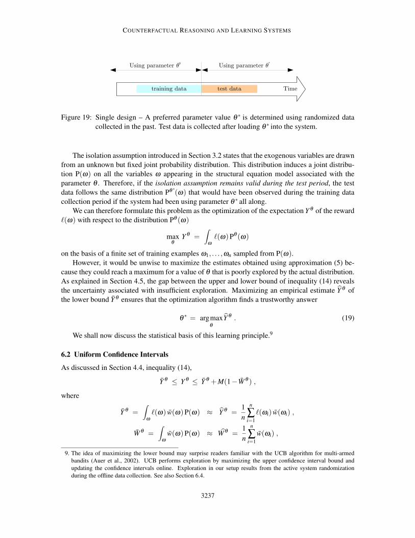
COUNTERFACTUAL REASONING AND LEARNING SYSTEMS
Figure 19: Single design – A preferred parameter value θ ∗ is determined using randomized datacollected in the past. Test data is collected after loading θ ∗ into the system.
The isolation assumption introduced in Section 3.2 states that the exogenous variables are drawnfrom an unknown but fixed joint probability distribution. This distribution induces a joint distribu-tion P(ω) on all the variables ω appearing in the structural equation model associated with theparameter θ . Therefore, if the isolation assumption remains valid during the test period, the testdata follows the same distribution Pθ ∗(ω) that would have been observed during the training datacollection period if the system had been using parameter θ ∗ all along.
We can therefore formulate this problem as the optimization of the expectation Y θ of the reward`(ω) with respect to the distribution Pθ (ω)
maxθ
Y θ =∫
ω
`(ω)Pθ (ω)
on the basis of a finite set of training examples ω1, . . . ,ωn sampled from P(ω).However, it would be unwise to maximize the estimates obtained using approximation (5) be-
cause they could reach a maximum for a value of θ that is poorly explored by the actual distribution.As explained in Section 4.5, the gap between the upper and lower bound of inequality (14) revealsthe uncertainty associated with insufficient exploration. Maximizing an empirical estimate Y θ ofthe lower bound Y θ ensures that the optimization algorithm finds a trustworthy answer
θ∗ = argmax
θ
Y θ . (19)
We shall now discuss the statistical basis of this learning principle.9
6.2 Uniform Confidence Intervals
As discussed in Section 4.4, inequality (14),
Y θ ≤ Y θ ≤ Y θ +M(1−W θ ) ,
where
Y θ =∫
ω
`(ω) w(ω)P(ω) ≈ Y θ =1n
n
∑i=1
`(ωi) w(ωi) ,
W θ =∫
ω
w(ω)P(ω) ≈ W θ =1n
n
∑i=1
w(ωi) ,
9. The idea of maximizing the lower bound may surprise readers familiar with the UCB algorithm for multi-armedbandits (Auer et al., 2002). UCB performs exploration by maximizing the upper confidence interval bound andupdating the confidence intervals online. Exploration in our setup results from the active system randomizationduring the offline data collection. See also Section 6.4.
3237

BOTTOU, PETERS, ET AL.
leads to confidence intervals (15) of the form
∀δ > 0, ∀θ P
Y θ − εR ≤ Y θ ≤ Y θ +M(1−W θ +ξR)+ εR
≥ 1−δ . (20)
Both εR and ξR converge to zero in inverse proportion to the square root of the sample size n. Theyalso increase at most linearly in logδ and depend on both the capping bound R and the parameter θ
through the empirical variances (see appendix B.)Such confidence intervals are insufficient to provide guarantees for a parameter value θ ∗ that
depends on the sample. In fact, the optimization (19) procedure is likely to select values of θ
for which the inequality is violated. We therefore seek uniform confidence intervals (Vapnik andChervonenkis, 1968), simultaneously valid for all values of θ .
• When the parameter θ is chosen from a finite set F , applying the union bound to the ordinaryintervals (20) immediately gives the uniform confidence interval :
P∀θ ∈F , Y θ−εR ≤ Y θ ≤ Y θ+M(1−W θ+ξR)+εR
≥ 1−|F |δ .
• Following the pioneering work of Vapnik and Chervonenkis, a broad choice of mathematicaltools have been developed to construct uniform confidence intervals when the set F is in-finite. For instance, appendix E leverages uniform empirical Bernstein bounds (Maurer andPontil, 2009) and obtains the uniform confidence interval
P∀θ ∈F , Y θ−εR ≤ Y θ ≤ Y θ+M(1−W θ+ξR)+εR
≥ 1−M (n)δ , (21)
where the growth function M (n) measures the capacity of the family of functions
fθ : ω 7→ `(ω)w(ω) , gθ : ω 7→ w(ω) , ∀θ ∈F .
Many practical choices of P∗(ω) lead to functions M (n) that grow polynomially with thesample size. Because both εR and ξR are O(n−1/2 logδ ), they converge to zero with the samplesize when one maintains the confidence level 1−M (n)δ equal to a predefined constant.
The interpretation of the inner and outer confidence intervals (Section 4.5) also applies to theuniform confidence interval (21). When the sample size is sufficiently large and the capping bound Rchosen appropriately, the inner confidence interval reflects the upper and lower bound of inequal-ity (14).
The uniform confidence interval therefore ensures that Y θ ∗ is close to the maximum of the lowerbound of inequality (14) which essentially represents the best performance that can be guaranteedusing training data sampled from P(ω). Meanwhile, the upper bound of this same inequality revealswhich values of θ could potentially offer better performance but have been insufficiently probed bythe sampling distribution (Figure 20.)
6.3 Tuning Ad Placement Auctions
We now present an application of this learning principle to the optimization of auction tuning pa-rameters in the ad placement engine. Despite increasingly challenging engineering difficulties,comparable optimization procedures can obviously be applied to larger numbers of tunable param-eters.
3238
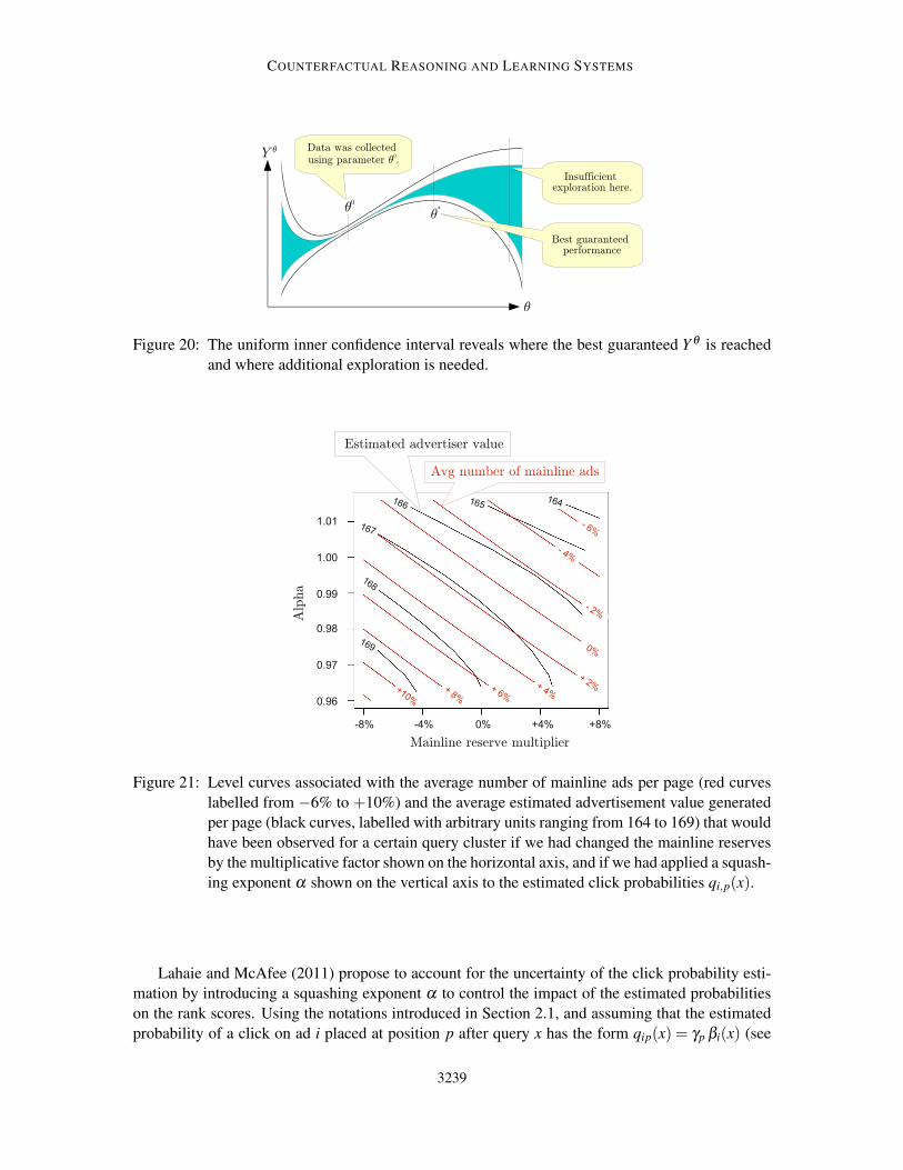
COUNTERFACTUAL REASONING AND LEARNING SYSTEMS
Figure 20: The uniform inner confidence interval reveals where the best guaranteed Y θ is reachedand where additional exploration is needed.
Figure 21: Level curves associated with the average number of mainline ads per page (red curveslabelled from −6% to +10%) and the average estimated advertisement value generatedper page (black curves, labelled with arbitrary units ranging from 164 to 169) that wouldhave been observed for a certain query cluster if we had changed the mainline reservesby the multiplicative factor shown on the horizontal axis, and if we had applied a squash-ing exponent α shown on the vertical axis to the estimated click probabilities qi,p(x).
Lahaie and McAfee (2011) propose to account for the uncertainty of the click probability esti-mation by introducing a squashing exponent α to control the impact of the estimated probabilitieson the rank scores. Using the notations introduced in Section 2.1, and assuming that the estimatedprobability of a click on ad i placed at position p after query x has the form qip(x) = γp βi(x) (see
3239
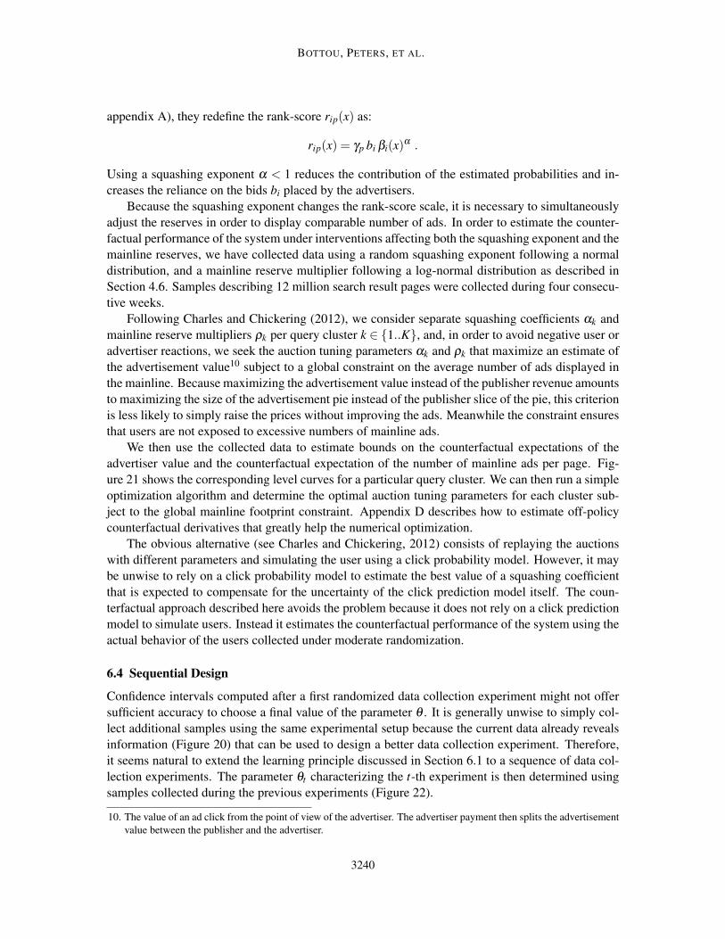
BOTTOU, PETERS, ET AL.
appendix A), they redefine the rank-score rip(x) as:
rip(x) = γp bi βi(x)α .
Using a squashing exponent α < 1 reduces the contribution of the estimated probabilities and in-creases the reliance on the bids bi placed by the advertisers.
Because the squashing exponent changes the rank-score scale, it is necessary to simultaneouslyadjust the reserves in order to display comparable number of ads. In order to estimate the counter-factual performance of the system under interventions affecting both the squashing exponent and themainline reserves, we have collected data using a random squashing exponent following a normaldistribution, and a mainline reserve multiplier following a log-normal distribution as described inSection 4.6. Samples describing 12 million search result pages were collected during four consecu-tive weeks.
Following Charles and Chickering (2012), we consider separate squashing coefficients αk andmainline reserve multipliers ρk per query cluster k ∈ 1..K, and, in order to avoid negative user oradvertiser reactions, we seek the auction tuning parameters αk and ρk that maximize an estimate ofthe advertisement value10 subject to a global constraint on the average number of ads displayed inthe mainline. Because maximizing the advertisement value instead of the publisher revenue amountsto maximizing the size of the advertisement pie instead of the publisher slice of the pie, this criterionis less likely to simply raise the prices without improving the ads. Meanwhile the constraint ensuresthat users are not exposed to excessive numbers of mainline ads.
We then use the collected data to estimate bounds on the counterfactual expectations of theadvertiser value and the counterfactual expectation of the number of mainline ads per page. Fig-ure 21 shows the corresponding level curves for a particular query cluster. We can then run a simpleoptimization algorithm and determine the optimal auction tuning parameters for each cluster sub-ject to the global mainline footprint constraint. Appendix D describes how to estimate off-policycounterfactual derivatives that greatly help the numerical optimization.
The obvious alternative (see Charles and Chickering, 2012) consists of replaying the auctionswith different parameters and simulating the user using a click probability model. However, it maybe unwise to rely on a click probability model to estimate the best value of a squashing coefficientthat is expected to compensate for the uncertainty of the click prediction model itself. The coun-terfactual approach described here avoids the problem because it does not rely on a click predictionmodel to simulate users. Instead it estimates the counterfactual performance of the system using theactual behavior of the users collected under moderate randomization.
6.4 Sequential Design
Confidence intervals computed after a first randomized data collection experiment might not offersufficient accuracy to choose a final value of the parameter θ . It is generally unwise to simply col-lect additional samples using the same experimental setup because the current data already revealsinformation (Figure 20) that can be used to design a better data collection experiment. Therefore,it seems natural to extend the learning principle discussed in Section 6.1 to a sequence of data col-lection experiments. The parameter θt characterizing the t-th experiment is then determined usingsamples collected during the previous experiments (Figure 22).
10. The value of an ad click from the point of view of the advertiser. The advertiser payment then splits the advertisementvalue between the publisher and the advertiser.
3240

COUNTERFACTUAL REASONING AND LEARNING SYSTEMS
Figure 22: Sequential design – The parameter θt of each data collection experiment is determinedusing data collected during the previous experiments.
Although it is relatively easy to construct convergent sequential design algorithms, reaching theoptimal learning performance is notoriously difficult (Wald, 1945) because the selection of param-eter θt involves a trade-off between exploitation, that is, the maximization of the immediate rewardY θt , and exploration, that is, the collection of samples potentially leading to better Y θ in the moredistant future.
The optimal exploration exploitation trade-off for multi-armed bandits is well understood (Git-tins, 1989; Auer et al., 2002; Audibert et al., 2007) because an essential property of multi-armedbandits makes the analysis much simpler: the outcome observed after performing a particular actionbrings no information about the value of other actions. Such an assumption is both unrealistic andpessimistic. For instance, the outcome observed after displaying a certain ad in response to a certainquery brings very useful information about the value of displaying similar ads on similar queries.
Refined contextual bandit approaches (Slivkins, 2011) account for similarities in the context andaction spaces but do not take advantage of all the additional opportunities expressed by structuralequation models. For instance, in the contextual bandit formulation of the ad placement problemoutlined in Section 3.5, actions are pairs (s,c) describing the ad slate s and the corresponding clickprices c, policies select actions by combining individual ad scores in very specific ways, and actionsdetermine the rewards through very specific mechanisms.
Meanwhile, despite their suboptimal asymptotic properties, heuristic exploration strategies per-form surprisingly well during the time span in which the problem can be considered stationary.Even in the simple case of multi-armed bandits, excellent empirical results have been obtained us-ing Thompson sampling (Chapelle and Li, 2011) or fixed strategies (Vermorel and Mohri, 2005;Kuleshov and Precup, 2010). Leveraging the problem structure seems more important in practicethan perfecting an otherwise sound exploration strategy.
Therefore, in the absence of sufficient theoretical guidance, it is both expedient and practical tomaximizing Y θ at each round, as described in Section 6.1, subject to additional ad-hoc constraintsensuring a minimum level of exploration.
7. Equilibrium Analysis
All the methods discussed in this contribution rely on the isolation assumption presented in Sec-tion 3.2. This assumption lets us interpret the samples as repeated independent trials that follow thepattern defined by the structural equation model and are amenable to statistical analysis.
The isolation assumption is in fact a component of the counterfactual conditions under inves-tigation. For instance, in Section 4.6, we model single auctions (Figure 3) in order to empirically
3241

BOTTOU, PETERS, ET AL.
determine how the ad placement system would have performed if we had changed the mainlinereserves without incurring a reaction from the users or the advertisers.
Since the future publisher revenues depend on the continued satisfaction of users and advertisers,lifting this restriction is highly desirable.
• We can in principle work with larger structural equation models. For instance, Figure 4suggests to thread single auction models with additional causal links representing the impactof the displayed ads on the future user goodwill. However, there are practical limits on thenumber of trials we can consider at once. For instance, it is relatively easy to simultaneouslymodel all the auctions associated with the web pages served to the same user during a thirtyminute web session. On the other hand, it is practically impossible to consider several weeksworth of auctions in order to model their accumulated effect on the continued satisfaction ofusers and advertisers.
• We can sometimes use problem-specific knowledge to construct alternate performance met-rics that anticipate the future effects of the feedback loops. For instance, in Section 6.3, weoptimize the advertisement value instead of the publisher revenue. Since this alternative cri-terion takes the advertiser interests into account, it can be viewed as a heuristic proxy for thefuture revenues of the publisher.
This section proposes an alternative way to account for such feedback loops using the quasistaticequilibrium method familiar to physicists: we assume that the publisher changes the parameter θ
so slowly that the system remains at equilibrium at all times. Using data collected while the systemwas at equilibrium, we describe empirical methods to determine how an infinitesimal interventiondθ on the model parameters would have displaced the equilibrium:
“How would the system have performed during the data collection period if a smallchange dθ had been applied to the model parameter θ and the equilibrium had beenreached before the data collection period.”
A learning algorithm can then update θ to improve selected performance metrics.
7.1 Rational Advertisers
The ad placement system is an example of game where each actor furthers his or her interests bycontrolling some aspects of the system: the publisher controls the placement engine parameters, theadvertisers control the bids, and the users control the clicks.
As an example of the general quasi-static approach, this section focuses on the reaction of ratio-nal advertisers to small changes of the scoring functions driving the ad placement system. Rationaladvertisers always select bids that maximize their economic interests. Although there are more re-alistic ways to model advertisers, this exercise is interesting because the auction theory approachesalso rely on the rational advertiser assumption (see Section 2.1). This analysis seamlessly integratesthe auction theory and machine learning perspectives.
As illustrated in Figure 23, we treat the bid vector b? = (b1 . . .bA) ∈ [0,bmax]A as the parameter
of the conditional distribution Pb?(b|x,v) of the bids associated with the eligible ads.11 The vari-
11. Quantities measured when a feedback causal system reaches equilibrium often display conditional independencepatterns that cannot be represented with directed acyclic graphs (Lauritzen and Richardson, 2002; Dash, 2003).Treating the feedback loop as parameters instead of variables works around this difficulty in a manner that appearssufficient to perform the quasi-static analysis.
3242
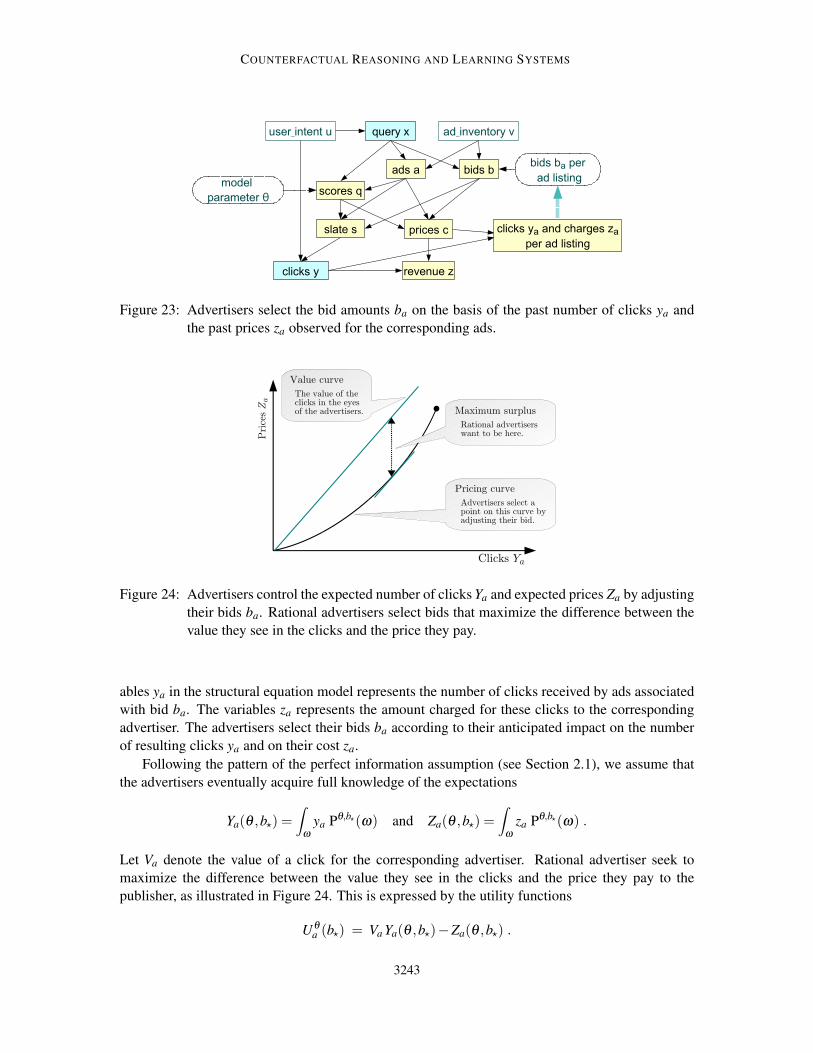
COUNTERFACTUAL REASONING AND LEARNING SYSTEMS
Figure 23: Advertisers select the bid amounts ba on the basis of the past number of clicks ya andthe past prices za observed for the corresponding ads.
!
Figure 24: Advertisers control the expected number of clicks Ya and expected prices Za by adjustingtheir bids ba. Rational advertisers select bids that maximize the difference between thevalue they see in the clicks and the price they pay.
ables ya in the structural equation model represents the number of clicks received by ads associatedwith bid ba. The variables za represents the amount charged for these clicks to the correspondingadvertiser. The advertisers select their bids ba according to their anticipated impact on the numberof resulting clicks ya and on their cost za.
Following the pattern of the perfect information assumption (see Section 2.1), we assume thatthe advertisers eventually acquire full knowledge of the expectations
Ya(θ ,b?) =∫
ω
ya Pθ,b?(ω) and Za(θ ,b?) =∫
ω
za Pθ,b?(ω) .
Let Va denote the value of a click for the corresponding advertiser. Rational advertiser seek tomaximize the difference between the value they see in the clicks and the price they pay to thepublisher, as illustrated in Figure 24. This is expressed by the utility functions
Uθa (b?) = Va Ya(θ ,b?)−Za(θ ,b?) .
3243
BOTTOU, PETERS, ET AL.
Following Athey and Nekipelov (2010), we argue that the injection of smooth random noiseinto the auction mechanism changes the discrete problem into a continuous problem amenable tostandard differential methods. Mild regularity assumption on the densities probability Pb?(b|x,v)and Pθ (q|x,a) are in fact sufficient to ensure that the expectations Ya(θ ,b?) and Za(θ ,b?) are con-tinuously differentiable functions of the distribution parameters b? and θ . Further assuming thatutility functions Uθ
a (b?) are diagonally quasiconcave, Athey and Nekipelov establish the existenceof a unique Nash equilibrium
∀a ba ∈ ArgMaxb
Uθa (b1, . . . ,ba−1,b,ba+1, . . . ,bA)
characterized by its first order Karush-Kuhn-Tucker conditions
∀a Va∂Ya
∂ba− ∂Za
∂ba
≤ 0 if ba = 0,≥ 0 if ba = bmax,= 0 if 0 < ba < bmax.
(22)
We use the first order equilibrium conditions (22) for two related purposes. Section 7.2 explainshow to complete the advertiser model by estimating the values Va. Section 7.3 estimates how theequilibrium bids and the system performance metrics respond to a small change dθ of the modelparameters.
Interestingly, this approach remains sensible when key assumptions of the equilibrium modelare violated. The perfect information assumption is unlikely to hold in practice. The quasi-concavityof the utility functions is merely plausible. However, after observing the operation of the stationaryad placement system for a sufficiently long time, it is reasonable to assume that the most activeadvertisers have tried small bid variations and have chosen locally optimal ones. Less active adver-tisers may leave their bids unchanged for longer time periods, but can also update them brutally ifthey experience a significant change in return on investment. Therefore it makes sense to use datacollected when the system is stationary to estimate advertiser values Va that are consistent with thefirst order equilibrium conditions. We then hope to maintain the conditions that each advertisers hadfound sufficiently attractive, by first estimating how a small change dθ displaces this posited localequilibrium, then by using performance metrics that take this displacement into account.
7.2 Estimating Advertiser Values
We first need to estimate the partial derivatives appearing in the equilibrium condition (22). Thesederivatives measure how the expectations Ya and Za would have been changed if each advertiser hadplaced a slightly different bid ba. Such quantities can be estimated by randomizing the bids andcomputing on-policy counterfactual derivatives as explained in appendix D. Confidence intervalscan be derived with the usual tools.
Unfortunately, the publisher is not allowed to directly randomize the bids because the advertisersexpect to pay prices computed using the bid they have specified and not the potentially higher bidsresulting from the randomization. However, the publisher has full control on the estimated clickprobabilities qi,p(x). Since the rank-scores ri,p(x) are the products of the bids and the estimated clickprobabilities (see Section 2.1), a random multiplier applied to the bids can also be interpreted as arandom multiplier applied to the estimated click probabilities. Under these two interpretations, thesame ads are shown to the users, but different click prices are charged to the advertisers. Therefore,
3244
COUNTERFACTUAL REASONING AND LEARNING SYSTEMS
the publisher can simultaneously charge prices computed as if the multiplier had been applied to theestimated click probabilities, and collect data as if the multiplier had been applied to the bid. Thisdata can then be used to estimate the derivatives.
Solving the first order equilibrium equations then yields estimated advertiser values Va that areconsistent with the observed data.12
[Corrected 9/9/2014]Va ≈∂Za
∂ba
/∂Ya
∂ba
There are however a couple caveats:
• The advertiser bid ba may be too small to cause ads to be displayed. In the absence of data,we have no means to estimate a click value for these advertisers.
• Many ads are not displayed often enough to obtain accurate estimates of the partial derivatives∂Ya∂ba
and ∂Za∂ba
. This can be partially remediated by smartly aggregating the data of advertisersdeemed similar.
• Some advertisers attempt to capture all the available ad opportunities by placing extremelyhigh bids and hoping to pay reasonable prices thanks to the generalized second price rule.Both partial derivatives ∂Ya
∂baand ∂Za
∂baare equal to zero in such cases. Therefore we cannot
recover Va by solving the equilibrium Equation (22). It is however possible to collect usefuldata by selecting for these advertisers a maximum bid bmax that prevents them from monop-olizing the eligible ad opportunities. Since the equilibrium condition is an inequality whenba = bmax, we can only determine a lower bound of the values Va for these advertisers.
These caveats in fact underline the limitations of the advertiser modelling assumptions. When theirads are not displayed often enough, advertisers have no more chance to acquire a full knowledgeof the expectations Ya and Za than the publisher has a chance to determine their value. Similarly,advertisers that place extremely high bids are probably underestimating the risk to occasionallyexperience a very high click price. A more realistic model of the advertiser information acquisitionis required to adequately handle these cases.
7.3 Estimating the Equilibrium Response
Let A be the set of the active advertisers, that is, the advertisers whose value can be estimated(or lower bounded) with sufficient accuracy. Assuming that the other advertisers leave their bidsunchanged, we can estimate how the active advertisers adjust their bids in response to an infinitesi-mal change dθ of the scoring model parameters. This is achieved by differentiating the equilibriumequations (22):
∀a′ ∈A , 0 =
(Va′
∂ 2Ya′
∂ba′ ∂θ− ∂ 2Za′
∂ba′ ∂θ
)dθ + ∑
a∈A
(Va′
∂ 2Ya′
∂ba′ ∂ba− ∂ 2Za′
∂ba′ ∂ba
)dba . (23)
The partial second derivatives must be estimated as described in appendix D. Solving this linearsystem of equations then yields an expression of the form
dba = Ξa dθ .
12. This approach is of course related to the value estimation method proposed by Athey and Nekipelov (2010) but strictlyrelies on the explicit randomization of the scores. In contrast, practical considerations force Athey and Nekipelov torely on the apparent noise and hope that the noise model accounts for all potential confounding factors.
3245
BOTTOU, PETERS, ET AL.
This expression can then be used to estimate how any counterfactual expectation Y of interestchanges when the publisher applies an infinitesimal change dθ to the scoring parameter θ andthe active advertisers A rationally adjust their bids ba in response:
dY =
(∂Y∂θ
+ ∑a
Ξa∂Y∂ba
)dθ . (24)
Although this expression provides useful information, one should remain aware of its limita-tions. Because we only can estimate the reaction of active advertisers, expression (24) does notincludes the potentially positive reactions of advertisers who did not bid but could have. Becausewe only can estimate a lower bound of their values, this expression does not model the potential re-actions of advertisers placing unrealistically high bids. Furthermore, one needs to be very cautiouswhen the system (23) approaches singularities. Singularities indicate that the rational advertiserassumption is no longer sufficient to determine the reactions of certain advertisers. This happens forinstance when advertisers cannot find bids that deliver a satisfactory return. The eventual behaviorof such advertisers then depends on factors not taken in consideration by our model.
To alleviate these issues, we could alter the auction mechanism in a manner that forces advertis-ers to reveal more information, and we could enforce policies ensuring that the system (23) remainssafely nonsingular. We could also design experiments revealing the impact of the fixed costs in-curred by advertisers participating into new auctions. Although additional work is needed to designsuch refinements, the quasistatic equilibrium approach provides a generic framework to take suchaspects into account.
7.4 Discussion
The rational advertiser assumption is the cornerstone of seminal works describing simplified vari-ants of the ad placement problem using auction theory (Varian, 2007; Edelman et al., 2007). Moresophisticated works account for more aspects of the ad placement problem, such as the impact ofclick prediction learning algorithms (Lahaie and McAfee, 2011), the repeated nature of the ad auc-tions (Bergemann and Said, 2010), or for the fact that advertisers place bids valid for multiple auc-tions (Athey and Nekipelov, 2010). Despite these advances, it seems technically very challengingto use these methods and account for all the effects that can be observed in practical ad placementsystems.
We believe that our counterfactual reasoning framework is best viewed as a modular toolkitthat lets us apply insights from auction theory and machine learning to problems that are far morecomplex than those studied in any single paper. For instance, the quasi-static equilibrium analysistechnique illustrated in this section extends naturally to the analysis of multiple simultaneous causalfeedback loops involving additional players:
• The first step consists in designing ad-hoc experiments to identify the parameters that deter-mine the equilibrium equation of each player. In the case of the advertisers, we have shownhow to use randomized scores to reveal the advertiser values. In the case of the user feedback,we must carefully design experiments that reveal how users respond to changes in the qualityof the displayed ads.
• Differentiating all the equilibrium equations yields a linear system of equations linking thevariations of the parameter under our control, such as dθ , and all the parameters under the
3246

COUNTERFACTUAL REASONING AND LEARNING SYSTEMS
control of the other players, such as the advertiser bids, or the user willingness to visit thesite and click on ads. Solving this system and writing the total derivative of the performancemeasure gives the answer to our question.
Although this programme has not yet been fully realized, the existence of a principled frame-work to handle such complex interactions is remarkable. Furthermore, thanks to the flexibility ofthe causal inference frameworks, these techniques can be infinitely adapted to various modelingassumptions and various system complexities.
8. Conclusion
Using the ad placement example, this work demonstrates the central role of causal inference (Pearl,2000; Spirtes et al., 1993) for the design of learning systems interacting with their environment.Thanks to importance sampling techniques, data collected during randomized experiments givesprecious cues to assist the designer of such learning systems and useful signals to drive learningalgorithms.
Two recurrent themes structure this work. First, we maintain a sharp distinction between thelearning algorithms and the extraction of the signals that drive them. Since real world learningsystems often involve a mixture of human decision and automated processes, it makes sense toseparate the discussion of the learning signals from the discussion of the learning algorithms thatleverage them. Second, we claim that the mathematical and philosophical tools developed for theanalysis of physical systems appear very effective for the analysis of causal information systemsand of their equilibria. These two themes are in fact a vindication of cybernetics (Wiener, 1948).
Acknowledgments
We would like to acknowledge extensive discussions with Susan Athey, Miroslav Dudík, PatrickJordan, John Langford, Lihong Li, Sebastien Lahaie, Shie Mannor, Chris Meek, Alex Slivkins, andPaul Viola. We also thank the Microsoft adCenter RnR team for giving us the invaluable opportunityto deploy these ideas at scale and prove their worth. Finally we gratefully acknowledge the preciouscomments of our JMLR editor and reviewers.
Appendix A. Greedy Ad Placement Algorithms
Section 2.1 describes how to select and place ads on a web page by maximizing the total rank-score (1). Following (Varian, 2007; Edelman et al., 2007) , we assume that the click probabilityestimates are expressed as the product of a positive position term γp and a positive ad term βi(x).The rank-scores can therefore be written as ri,p(x) = γpbiβi(x). We also assume that the policyconstraints simply state that a web page should not display more than one ad belonging to any givenadvertiser. The discrete maximization problem is then amenable to computationally efficient greedyalgorithms.
Let us fix a layout L and focus on the inner maximization problem. Without loss of generality,we can renumber the positions such that
L = 1,2, . . .N and γ1 ≥ γ2 ≥ ·· · ≥ 0 .
3247
BOTTOU, PETERS, ET AL.
and write the inner maximization problem as
maxi1,...,iN
RL(i1, . . . , iN) = ∑p∈L
rip,p(x)
subject to the policy constraints and reserve constraints ri,p(x)≥ Rp(x).Let Si denote the advertiser owning ad i. The set of ads is then partitioned into subsets Is =
i : Si = s gathering the ads belonging to the same advertiser s. The ads that maximize the productbiβi(x) within set Is are called the best ads for advertiser s. If the solution of the discrete maxi-mization problem contains one ad belonging to advertiser s, then it is easy to see that this ad mustbe one of the best ads for advertiser s: were it not the case, replacing the offending ad by one of thebest ads would yield a higher RL without violating any of the constraints. It is also easy to see thatone could select any of the best ads for advertiser s without changing RL.
Let the set I ∗ contain exactly one ad per advertiser, arbitrarily chosen among the best ads forthis advertiser. The inner maximization problem can then be simplified as:
maxi1,...,iN∈I ∗
RL(i1, . . . , iN) = ∑p∈L
γp bip βip(x)
where all the indices i1, . . . , iN are distinct, and subject to the reserve constraints.Assume that this maximization problem has a solution i1, . . . , iN , meaning that there is a feasible
ad placement solution for the layout L. For k = 1 . . .N, let us define I∗k ⊂I ∗ as
I∗k = ArgMaxi∈I ∗\i1,...,ik−1
biβi(x) .
It is easy to see that I∗k intersects ik, . . . , iN because, were it not the case, replacing ik by anyelement of I∗k would increase RL without violating any of the constraints. Furthermore it is easy tosee that ik ∈ I∗k because, were it not the case, there would be h > k such that ih ∈ I∗k , and swappingik and ih would increase RL without violating any of the constraints.
Therefore, if the inner maximization problem admits a solution, we can compute a solutionby recursively picking i1, . . . , iN from I∗1 , I
∗2 , . . . , I
∗N . This can be done efficiently by first sorting
the biβi(x) in decreasing order, and then greedily assigning ads to the best positions subject to thereserve constraints. This operation has to be repeated for all possible layouts, including of coursethe empty layout.
The same analysis can be carried out for click prediction estimates expressed as arbitrary mono-tone combination of a position term γp(x) and an ad term βi(x), as shown, for instance, by Graepelet al. (2010).
Appendix B. Confidence Intervals
Section 4.4 explains how to obtain improved confidence intervals by replacing the unbiased impor-tance sampling estimator (7) by the clipped importance sampling estimator (10). This appendixprovides details that could have obscured the main message.
3248

COUNTERFACTUAL REASONING AND LEARNING SYSTEMS
B.1 Outer Confidence Interval
We first address the computation of the outer confidence interval (12) which describes how theestimator Y ∗ approaches the clipped expectation Y ∗.
Y ∗ =∫
ω
`(ω) w(ω) P(ω) ≈ Y ∗ =1n
n
∑i=1
`(ωi) w(ωi) .
Since the samples `(ωi) w(ωi) are independent and identically distributed, the central limit theorem(e.g., Cramér, 1946, Section 17.4) states that the empirical average Y ∗ converges in law to a normaldistribution of mean Y ∗ = E[`(ω) w(ω)] and variance V = var[`(ω) w(ω)]. Since this convergenceusually occurs quickly, it is widely accepted to write
P
Y ∗− εR ≤ Y ∗ ≤ Y ∗+ εR
≥ 1−δ ,
withεR = erf
−1(1−δ )
√2V . (25)
and to estimate the variance V using the sample variance V
V ≈ V =1
n−1
n
∑i=1
(`(ωi) w(ωi)− Y ∗
)2.
This approach works well when the ratio ceiling R is relatively small. However the presence of afew very large ratios makes the variance estimation noisy and might slow down the central limitconvergence.
The first remedy is to bound the variance more rigorously. For instance, the following boundresults from (Maurer and Pontil, 2009, Theorem 10).
P√
V >√
V + (M−m)R
√2log(2/δ )
n−1
≤ δ
Combining this bound with (25) gives a confidence interval valid with probability greater than1−2δ . Although this approach eliminates the potential problems related to the variance estimation,it does not address the potentially slow convergence of the central limit theorem.
The next remedy is to rely on empirical Bernstein bounds to derive rigorous confidence intervalsthat leverage both the sample mean and the sample variance (Audibert et al., 2007; Maurer andPontil, 2009).
Theorem 1 (Empirical Bernstein bound) (Maurer and Pontil, 2009, thm 4)Let X ,X1,X2, . . . ,Xn be i.i.d. random variable with values in [a,b] and let δ > 0. Then, with proba-bility at least 1−δ ,
E[X ]−Mn ≤√
2Vn log(2/δ )
n+(b−a)
7log(2/δ )
3(n−1),
where Mn and Vn respectively are the sample mean and variance
Mn =1n
n
∑i=1
Xi , Vn =1
n−1
n
∑i=1
(Xi−Mn)2 .
3249

BOTTOU, PETERS, ET AL.
Applying this theorem to both `(ωi) w(ωi) and −`(ωi) w(ωi) provides confidence intervals thathold for for the worst possible distribution of the variables `(ω) and w(ω).
P
Y ∗− εR ≤ Y ∗ ≤ Y ∗+ εR
≥ 1−2δ
where
εR =
√2V log(2/δ )
n+M R
7log(2/δ )
3(n−1). (26)
Because they hold for the worst possible distribution, confidence intervals obtained in this wayare less tight than confidence intervals based on the central limit theorem. On the other hand, thanksto the Bernstein bound, they remains reasonably competitive, and they provide a much strongerguarantee.
B.2 Inner Confidence Interval
Inner confidence intervals are derived from inequality (14) which bounds the difference between thecounterfactual expectation Y ∗ and the clipped expectation Y ∗ :
0 ≤ Y ∗− Y ∗ ≤ M (1−W ∗) .
The constant M is defined by assumption (8). The first step of the derivation consists in obtaining alower bound of W ∗−W ∗ using either the central limit theorem or an empirical Bernstein bound.
For instance, applying theorem 1 to −w(ωi) yields
P
W ∗ ≥ W ∗−
√2Vw log(2/δ )
n−R
7log(2/δ )
3(n−1)
≥ 1−δ
where Vw is the sample variance of the clipped weights
Vw =1
n−1
n
∑i=1
(w(ωi)−W ∗
)2.
Replacing in inequality (14) gives the outer confidence interval
P
Y ∗ ≤ Y ∗ ≤ Y ∗+M(1−W ∗+ξR)≥ 1−δ .
with
ξR =
√2Vw log(2/δ )
n+R
7log(2/δ )
3(n−1). (27)
Note that 1−W + ξR can occasionally be negative. This occurs in the unlucky cases where theconfidence interval is violated, with probability smaller than δ .
Putting together the inner and outer confidence intervals,
P
Y ∗− εR ≤ Y ∗ ≤ Y ∗+M(1−W ∗+ξR)+ εR
≥ 1−3δ ,
with εR and ξR computed as described in expressions (26) and (27).
3250
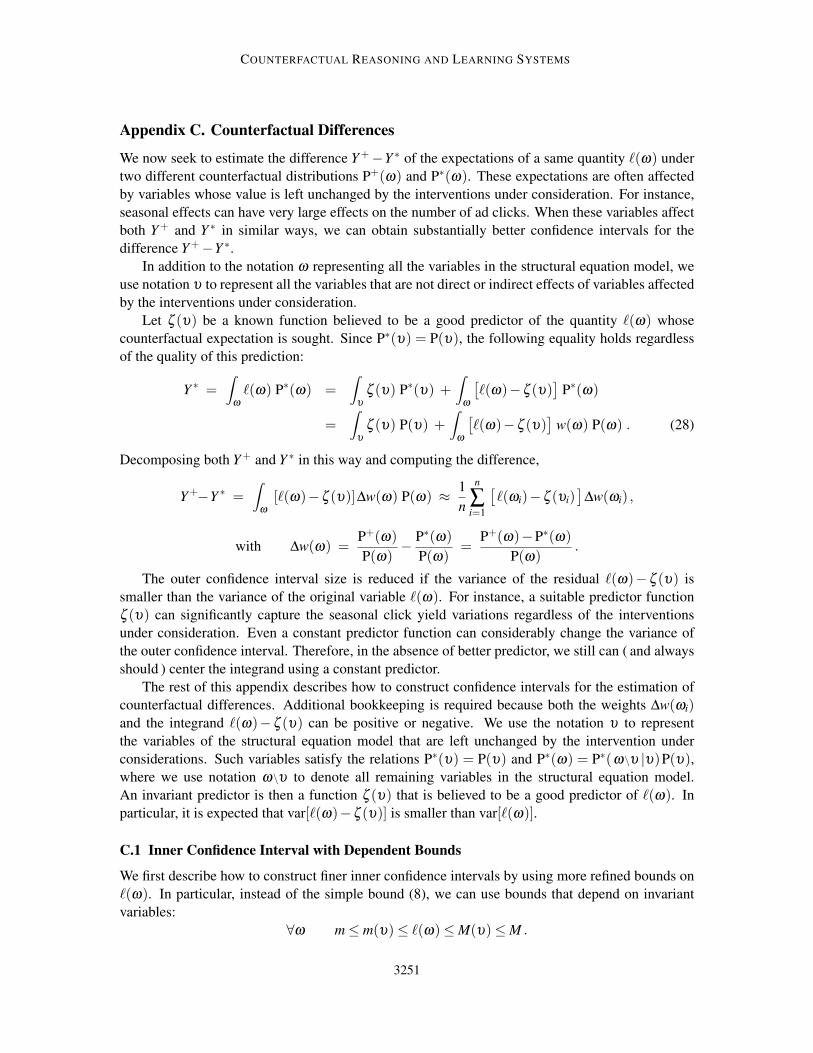
COUNTERFACTUAL REASONING AND LEARNING SYSTEMS
Appendix C. Counterfactual Differences
We now seek to estimate the difference Y+−Y ∗ of the expectations of a same quantity `(ω) undertwo different counterfactual distributions P+(ω) and P∗(ω). These expectations are often affectedby variables whose value is left unchanged by the interventions under consideration. For instance,seasonal effects can have very large effects on the number of ad clicks. When these variables affectboth Y+ and Y ∗ in similar ways, we can obtain substantially better confidence intervals for thedifference Y+−Y ∗.
In addition to the notation ω representing all the variables in the structural equation model, weuse notation υ to represent all the variables that are not direct or indirect effects of variables affectedby the interventions under consideration.
Let ζ (υ) be a known function believed to be a good predictor of the quantity `(ω) whosecounterfactual expectation is sought. Since P∗(υ) = P(υ), the following equality holds regardlessof the quality of this prediction:
Y ∗ =∫
ω
`(ω) P∗(ω) =∫
υ
ζ (υ) P∗(υ) +∫
ω
[`(ω)−ζ (υ)
]P∗(ω)
=∫
υ
ζ (υ) P(υ) +∫
ω
[`(ω)−ζ (υ)
]w(ω) P(ω) . (28)
Decomposing both Y+ and Y ∗ in this way and computing the difference,
Y+−Y ∗ =∫
ω
[`(ω)−ζ (υ)]∆w(ω) P(ω) ≈ 1n
n
∑i=1
[`(ωi)−ζ (υi)
]∆w(ωi) ,
with ∆w(ω) =P+(ω)
P(ω)− P∗(ω)
P(ω)=
P+(ω)−P∗(ω)
P(ω).
The outer confidence interval size is reduced if the variance of the residual `(ω)−ζ (υ) issmaller than the variance of the original variable `(ω). For instance, a suitable predictor functionζ (υ) can significantly capture the seasonal click yield variations regardless of the interventionsunder consideration. Even a constant predictor function can considerably change the variance ofthe outer confidence interval. Therefore, in the absence of better predictor, we still can ( and alwaysshould ) center the integrand using a constant predictor.
The rest of this appendix describes how to construct confidence intervals for the estimation ofcounterfactual differences. Additional bookkeeping is required because both the weights ∆w(ωi)and the integrand `(ω)−ζ (υ) can be positive or negative. We use the notation υ to representthe variables of the structural equation model that are left unchanged by the intervention underconsiderations. Such variables satisfy the relations P∗(υ) = P(υ) and P∗(ω) = P∗(ω\υ |υ)P(υ),where we use notation ω\υ to denote all remaining variables in the structural equation model.An invariant predictor is then a function ζ (υ) that is believed to be a good predictor of `(ω). Inparticular, it is expected that var[`(ω)−ζ (υ)] is smaller than var[`(ω)].
C.1 Inner Confidence Interval with Dependent Bounds
We first describe how to construct finer inner confidence intervals by using more refined bounds on`(ω). In particular, instead of the simple bound (8), we can use bounds that depend on invariantvariables:
∀ω m≤ m(υ)≤ `(ω)≤M(υ)≤M .
3251

BOTTOU, PETERS, ET AL.
The key observation is the equality
E[w∗(ω)|υ ] =∫
ω\υw∗(ω) P(ω\υ |υ) =
∫ω\υ
P∗(ω\υ |υ)P(υ)P(ω\υ |υ)P(υ)
P(ω\υ |υ) = 1 .
We can then write
Y ∗− Y ∗ =∫
ω
[w∗(ω)− w∗(ω)
]`(ω) P(ω) ≤
∫υ
E[w∗(ω)− w∗(ω) |υ ] M(υ) P(υ)
=∫
υ
(1−E[w∗(ω)|υ ] ) M(υ) P(υ) =∫
ω
(1− w∗(ω)) M(υ) P(ω) = Bhi .
Using a similar derivation for the lower bound Blo, we obtain the inequality
Blo ≤ Y ∗− Y ∗ ≤ Bhi
With the notations
Blo =1n
n
∑i=1
(1− w∗(ωi))m(υi) , Bhi =1n
n
∑i=1
(1− w∗(ωi))M(υi) ,
Vlo =1
n−1
n
∑i=1
[(1−w∗(ωi))m(υi)− Blo
]2, Vhi =
1n−1
n
∑i=1
[(1−w∗(ωi))M(υi)− Bhi
]2,
ξlo =
√2Vlo log(2/δ )
n+ |m|R 7log(2/δ )
3(n−1), ξhi =
√2Vhi log(2/δ )
n+ |M|R 7log(2/δ )
3(n−1),
two applications of theorem 1 give the inner confidence interval:
P
Y ∗+ Blo−ξlo ≤ Y ∗ ≤ Y ∗+ Bhi +ξhi
≥ 1−2δ .
C.2 Confidence Intervals for Counterfactual Differences
We now describe how to leverage invariant predictors in order to construct tighter confidence inter-vals for the difference of two counterfactual expectations.
Y+−Y ∗ ≈ 1n
n
∑i=1
[`(ωi)−ζ (υi)
]∆w(ωi) with ∆w(ω) =
P+(ω)−P∗(ω)
P(ω).
Let us define the reweigthing ratios w+(ω) = P+(ω)/P(ω) and w∗(ω) = P∗(ω)/P(ω), their clippedvariants w+(ω) and w∗(ω), and the clipped centered expectations
Y+c =
∫ω
[`(ω)−ζ (υ)] w+(ω)P(ω) and Y ∗c =∫
ω
[`(ω)−ζ (υ)] w∗(ω)P(ω) .
The outer confidence interval is obtained by applying the techniques of Section B.1 to
Y+c − Y ∗c =
∫ω
[ `(ω)−ζ (υ) ] [ w+(ω)− w∗(ω) ] P(ω) .
Since the weights w+− w∗ can be positive or negative, adding or removing a constant to `(ω)can considerably change the variance of the outer confidence interval. This means that one should
3252

COUNTERFACTUAL REASONING AND LEARNING SYSTEMS
always use a predictor. Even a constant predictor can vastly improve the outer confidence intervaldifference.
The inner confidence interval is then obtained by writing the difference(Y+−Y ∗
)−(Y+
c − Y ∗c)
=∫
ω
[`(ω)−ζ (υ)
] [w+(ω)− w+(ω)
]P(ω)
−∫
ω
[`(ω)−ζ (υ)
] [w∗(ω)− w∗(ω)
]P(ω)
and bounding both terms by leveraging υ-dependent bounds on the integrand:
∀ω −M ≤ −ζ (υ) ≤ `(ω)−ζ (υ) ≤ M−ζ (υ) ≤ M .
This can be achieved as shown in Section C.1.
Appendix D. Counterfactual Derivatives
We now consider interventions that depend on a continuous parameter θ . For instance, we mightwant to know what the performance of the ad placement engine would have been if we had useda parametrized scoring model. Let Pθ (ω) represent the counterfactual Markov factorization asso-ciated with this intervention. Let Y θ be the counterfactual expectation of `(ω) under distributionPθ .
Computing the derivative of (28) immediately gives
∂Y θ
∂θ=∫
w
[`(ω)−ζ (υ)
]w′θ (ω) P(ω) ≈ 1
n
n
∑i=1
[`(ωi)−ζ (υi)
]w′θ (ωi)
with wθ (ω) =Pθ (ω)
P(ω)and w′θ (ω) =
∂wθ (ω)
∂θ= wθ (ω)
∂ logPθ (ω)
∂θ. (29)
Replacing the expressions P(ω) and Pθ (ω) by the corresponding Markov factorizations givesmany opportunities to simplify the reweighting ratio w′
θ(ω). The term wθ (ω) simplifies as shown
in (6). The derivative of logPθ (ω) depends only on the factors parametrized by θ . Therefore, inorder to evaluate w′
θ(ω), we only need to know the few factors affected by the intervention.
Higher order derivatives can be estimated using the same approach. For instance,
∂ 2Y θ
∂θi ∂θ j=∫
w
[`(ω)−ζ (υ)
]w′′i j(ω) P(ω) ≈ 1
n
n
∑i=1
[`(ωi)−ζ (υi)
]w′′i j(ωi)
with w′′i j(ω) =∂ 2wθ (ω)
∂θi ∂θ j= wθ (ω)
∂ logPθ (ω)
∂θi
∂ logPθ (ω)
∂θ j+wθ (ω)
∂ 2logPθ (ω)
∂θi ∂θ j.
The second term in w′′i j(ω) vanishes when θi and θ j parametrize distinct factors in Pθ (ω).
D.1 Infinitesimal Interventions and Policy Gradient
Expression (29) becomes particularly attractive when P(ω) = Pθ (ω), that is, when one seeks deriva-tives that describe the effect of an infinitesimal intervention on the system from which the data wascollected. The resulting expression is then identical to the celebrated policy gradient (Aleksandrov
3253
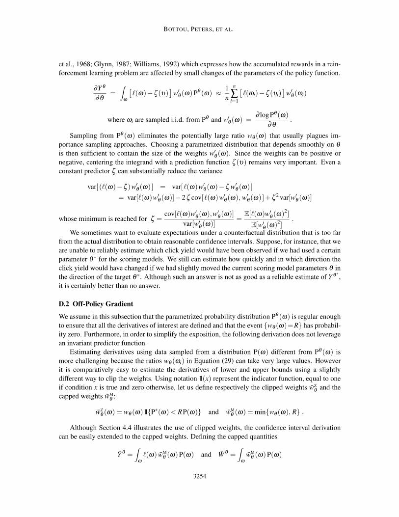
BOTTOU, PETERS, ET AL.
et al., 1968; Glynn, 1987; Williams, 1992) which expresses how the accumulated rewards in a rein-forcement learning problem are affected by small changes of the parameters of the policy function.
∂Y θ
∂θ=∫
ω
[`(ω)−ζ (υ)
]w′θ (ω)Pθ (ω) ≈ 1
n
n
∑i=1
[`(ωi)−ζ (υi)
]w′θ (ωi)
where ωi are sampled i.i.d. from Pθ and w′θ (ω) =∂ logPθ (ω)
∂θ.
Sampling from Pθ (ω) eliminates the potentially large ratio wθ (ω) that usually plagues im-portance sampling approaches. Choosing a parametrized distribution that depends smoothly on θ
is then sufficient to contain the size of the weights w′θ(ω). Since the weights can be positive or
negative, centering the integrand with a prediction function ζ (υ) remains very important. Even aconstant predictor ζ can substantially reduce the variance
var[ (`(ω)−ζ )w′θ (ω) ] = var[`(ω)w′θ (ω)−ζ w′θ (ω) ]
= var[`(ω)w′θ (ω)]−2ζ cov[`(ω)w′θ (ω), w′θ (ω) ]+ζ2 var[w′θ (ω)]
whose minimum is reached for ζ =cov[`(ω)w′
θ(ω),w′
θ(ω)]
var[w′θ(ω)]
=E[`(ω)w′
θ(ω)2]
E[w′θ(ω)2]
.
We sometimes want to evaluate expectations under a counterfactual distribution that is too farfrom the actual distribution to obtain reasonable confidence intervals. Suppose, for instance, that weare unable to reliably estimate which click yield would have been observed if we had used a certainparameter θ ∗ for the scoring models. We still can estimate how quickly and in which direction theclick yield would have changed if we had slightly moved the current scoring model parameters θ inthe direction of the target θ ∗. Although such an answer is not as good as a reliable estimate of Y θ ∗ ,it is certainly better than no answer.
D.2 Off-Policy Gradient
We assume in this subsection that the parametrized probability distribution Pθ (ω) is regular enoughto ensure that all the derivatives of interest are defined and that the event wθ (ω)=R has probabil-ity zero. Furthermore, in order to simplify the exposition, the following derivation does not leveragean invariant predictor function.
Estimating derivatives using data sampled from a distribution P(ω) different from Pθ (ω) ismore challenging because the ratios wθ (ωi) in Equation (29) can take very large values. Howeverit is comparatively easy to estimate the derivatives of lower and upper bounds using a slightlydifferent way to clip the weights. Using notation 1l(x) represent the indicator function, equal to oneif condition x is true and zero otherwise, let us define respectively the clipped weights wZ
θand the
capped weights wMθ
:
wZθ (ω) = wθ (ω)1lP∗(ω)< RP(ω) and wM
θ (ω) = minwθ (ω), R .
Although Section 4.4 illustrates the use of clipped weights, the confidence interval derivationcan be easily extended to the capped weights. Defining the capped quantities
Y θ =∫
ω
`(ω) wMθ (ω)P(ω) and W θ =
∫ω
wMθ (ω)P(ω)
3254
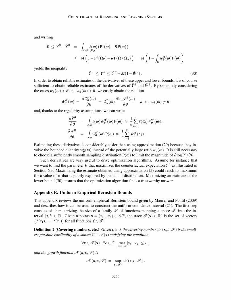
COUNTERFACTUAL REASONING AND LEARNING SYSTEMS
and writing
0 ≤ Y θ − Y θ =∫
ω∈Ω\ΩR
`(ω)(P∗(ω)−RP(ω))
≤ M(
1−P∗(ΩR)−RP(Ω\ΩR))
= M(
1−∫
ω
wMθ (ω)P(ω)
)yields the inequality
Y θ ≤ Y θ ≤ Y θ +M(1−W θ ) . (30)
In order to obtain reliable estimates of the derivatives of these upper and lower bounds, it is of coursesufficient to obtain reliable estimates of the derivatives of Y θ and W θ . By separately consideringthe cases wθ (ω)< R and wθ (ω)> R, we easily obtain the relation
wM′θ (ω) =
∂ wMθ(ω)
∂θ= wZ
θ (ω)∂ logPθ (ω)
∂θwhen wθ (ω) 6= R
and, thanks to the regularity assumptions, we can write
∂Y θ
∂θ=
∫ω
`(ω) wM′θ (ω)P(ω) ≈ 1
n
n
∑i=1
`(ωi) wM′θ (ωi) ,
∂W θ
∂θ=
∫ω
wM′θ (ω)P(ω) ≈ 1
n
n
∑i=1
wM′θ (ωi) ,
Estimating these derivatives is considerably easier than using approximation (29) because they in-volve the bounded quantity wZ
θ(ω) instead of the potentially large ratio wθ (ω). It is still necessary
to choose a sufficiently smooth sampling distribution P(ω) to limit the magnitude of ∂ logPθ/∂θ .Such derivatives are very useful to drive optimization algorithms. Assume for instance that
we want to find the parameter θ that maximizes the counterfactual expectation Y θ as illustrated inSection 6.3. Maximizing the estimate obtained using approximation (5) could reach its maximumfor a value of θ that is poorly explored by the actual distribution. Maximizing an estimate of thelower bound (30) ensures that the optimization algorithm finds a trustworthy answer.
Appendix E. Uniform Empirical Bernstein Bounds
This appendix reviews the uniform empirical Bernstein bound given by Maurer and Pontil (2009)and describes how it can be used to construct the uniform confidence interval (21). The first stepconsists of characterizing the size of a family F of functions mapping a space X into the in-terval [a,b] ⊂ R. Given n points x = (x1. . .xn) ∈X n, the trace F (x) ∈ Rn is the set of vectors(
f (x1), . . . , f (xn))
for all functions f ∈F .
Definition 2 (Covering numbers, etc.) Given ε > 0, the covering number N (x,ε,F ) is the small-est possible cardinality of a subset C ⊂F (x) satisfying the condition
∀v ∈F (x) ∃c ∈C maxi=1...n
|vi− ci| ≤ ε ,
and the growth function N (n,ε,F ) is
N (n,ε,F ) = supx∈X n
N (x,ε,F ) .
3255

BOTTOU, PETERS, ET AL.
Thanks to a famous combinatorial lemma (Vapnik and Chervonenkis, 1968, 1971; Sauer, 1972), formany usual parametric families F , the growth function N (n,ε,F ) increases at most polynomi-ally13 with both n and 1/ε .
Theorem 3 (Uniform empirical Bernstein bound) (Maurer and Pontil, 2009, thm 6)Let δ ∈ (0,1), n >= 16. Let X ,X1, . . . ,Xn be i.i.d. random variables with values in X . Let F be aset of functions mapping X into [a,b]⊂R and let M (n) = 10N (2n,F ,1/n). Then we probabilityat least 1−δ ,
∀ f ∈F , E[ f (X)]−Mn ≤√
18Vn log(M (n)/δ )
n+(b−a)
15 log(M (n)/δ )
n−1,
where Mn and Vn respectively are the sample mean and variance
Mn =1n
n
∑i=1
f (Xi) , Vn =1
n−1
n
∑i=1
( f (Xi)−Mn)2 .
The statement of this theorem emphasizes its similarity with the non-uniform empirical Bern-stein bound (theorem 1). Although the constants are less attractive, the uniform bound still con-verges to zero when n increases, provided of course that M (n) = 10N (2n,F ,1/n) grows polyno-mially with n.
Let us then define the family of functions
F = fθ : ω 7→ `(ω)wMθ (ω) , gθ : ω 7→ wM
θ (ω) , ∀θ ∈F ,
and use the uniform empirical Bernstein bound to derive an outer inequality similar to (26) and aninner inequality similar to (27). The theorem implies that, with probability 1−δ , both inequalitiesare simultaneously true for all values of the parameter θ . The uniform confidence interval (21) thenfollows directly.
References
V M. Aleksandrov, V. I. Sysoyev, and V. V. Shemeneva. Stochastic optimization. EngineeringCybernetics, 5:11–16, 1968.
Susan Athey and Denis Nekipelov. A structural model of sponsored search advertising. Working pa-per, 2010. URL http://kuznets.harvard.edu/~athey/papers/Structural_Sponsored_
Search.pdf.
Jean-Yves Audibert, Remi Munos, and Csaba Szepesvári. Tuning bandit algorithms in stochastic en-vironments. In Proc. 18th International Conference on Algorithmic Learning Theory (ALT 2007),pages 150–165, 2007.
Peter Auer, Nicolò Cesa-Bianchi, and Paul Fisher. Finite time analysis of the multiarmed banditproblem. Machine Learning, 47(2–3):235–256, 2002.
13. For a simple proof of this fact, slice [a,b] into intervals Sk of maximal width ε and apply the lemma to the family ofindicator functions (xi,Sk) 7→ 1l f (xi) ∈ Sk.
3256

COUNTERFACTUAL REASONING AND LEARNING SYSTEMS
Heejung Bang and James M. Robins. Doubly robust estimation in missing data and causal inferencemodels. Biometrics, 61:692–972, 2005.
Dirk Bergemann and Maher Said. Dynamic auctions: a survey. Discussion Paper 1757R, CowlesFoundation for Research in Economics, Yale University, 2010.
Léon Bottou. From machine learning to machine reasoning. http://arxiv.org/abs/1102.
1808v3, Feb 2011.
Leo Breiman. Statistical modeling: The two cultures. Statistical Science, 16(3):199–231, 2001.
Olivier Chapelle and Lihong Li. An empirical evaluation of thompson sampling. In Advances inNeural Information Processing Systems 24, pages 2249–2257. NIPS Foundation, 2011.
C. R. Charig, D. R. Webb, S. R. Payne, and J. E. A. Wickham. Comparison of treatment of renalcalculi by open surgery, percutaneous nephrolithotomy, and extracorporeal shockwave lithotripsy.British Medical Journal (Clin Res Ed), 292(6254):879–882, 1986.
Denis X. Charles and D. Max Chickering. Optimization for paid search auctions. Manuscript inpreparation, 2012.
Denis X. Charles, D. Max Chickering, and Patrice Simard. Micro-market experimentation for paidsearch. Manuscript in preparation, 2012.
Harald Cramér. Mathematical Methods of Statistics. Princeton University Press, 1946.
Denver Dash. Caveats for Causal Reasoning with Equilibrium Models. PhD thesis, University ofPittsburgh, 2003.
Miroslav Dudík, Dimitru Erhan, John Langford, and Lihong Li. Sample-efficient nonstationary-policy evaluation for contextual bandits. In Proceedings of Uncertainty in Artificial Intelligence(UAI), pages 247–254, 2012.
Benjamin Edelman, Michael Ostrovsky, and Michael Schwarz. Internet advertising and the gener-alized second price auction: Selling billions of dollars worth of keywords. American EconomicReview, 97(1):242–259, 2007.
Alan Genz. Numerical computation of multivariate normal probabilities. Journal Computation ofMultivariate Normal Probabilities, 1:141–149, 1992.
John C. Gittins. Bandit Processes and Dynamic Allocation Indices. Wiley, 1989.
Peter W. Glynn. Likelihood ratio gradient estimation: an overview. In Proceedings of the 1987Winter Simulation Conference, pages 366–375, 1987.
John Goodwin. Microsoft adCenter. Personal communication, 2011.
Thore Graepel, Joaquin Quinonero Candela, Thomas Borchert, and Ralf Herbrich. Web-scaleBayesian click-through rate prediction for sponsored search advertising in Microsoft’s Bingsearch engine. In Proceedings of the 27th International Conference on Machine Learning(ICML 2010), Invited Applications Track. Omnipress, 2010.
3257

BOTTOU, PETERS, ET AL.
Ron Kohavi, Roger Longbotham, Dan Sommerfield, and Randal M. Henne. Controlled experimentson the web: Survey and practical guide. Data Mining and Knowledge Discovery, 18(1):140–181,July 2008.
Volodymyr Kuleshov and Doina Precup. Algorithms for multi-armed bandit problems, October2010. http://www.cs.mcgill.ca/~vkules/bandits.pdf.
Sébastien Lahaie and R. Preston McAfee. Efficient ranking in sponsored search. In Proc. 7th In-ternational Workshop on Internet and Network Economics (WINE 2011), pages 254–265. LNCS7090, Springer, 2011.
Lev Landau and Evgeny Lifshitz. Course in Theoretical Physics, Volume 1: Mechanics. PergamonPress, 1969. 2nd edition.
John Langford and Tong Zhang. The epoch-greedy algorithm for multi-armed bandits with sideinformation. In Advances in Neural Information Processing Systems 20, pages 817–824. MITPress, Cambridge, MA, 2008.
Steffen L. Lauritzen and Thomas S. Richardson. Chain graph models and their causal interpretation.Journal of the Royal Statistical Society, Series B, 64:321–361, 2002.
David K. Lewis. Counterfactuals. Harvard University Press, 1973. 2nd edition: Wiley-Blackwell,2001.
Lihong Li, Wei Chu, John Langford, and Robert E. Schapire. A contextual-bandit approach topersonalized news article recommendation. In Proceedings of the 19th International Conferenceon the World Wide Web (WWW 2010), pages 661–670. ACM, 2010.
Lihong Li, Wei Chu, John Langford, and Xuanhui Wang. Unbiased offline evaluation of contextual-bandit-based news article recommendation algorithms. In Proc. 4th ACM International Confer-ence on Web Search and Data Mining (WSDM 2011), pages 297–306, 2011.
Andreas Maurer and Massimiliano Pontil. Empirical bernstein bounds and sample-variance penal-ization. In Proc. The 22nd Conference on Learning Theory (COLT 2009), 2009.
Paul Milgrom. Putting Auction Theory to Work. Cambridge University Press, 2004.
Roger B. Myerson. Optimal auction design. Mathematics of Operations Research, 6(1):58–73,1981.
Judea Pearl. Causality: Models, Reasoning, and Inference. Cambridge University Press, 2000. 2ndedition: 2009.
Judea Pearl. Causal inference in statistics: an overview. Statistics Surveys, 3:96–146, 2009.
Judea Pearl. The do-calculus revisited. In Proc. Twenty-Eighth Conference on Uncertainty inArtificial Intelligence (UAI-2012), pages 3–11, 2012.
Linda E. Reichl. A Modern Course in Statistical Physics, 2nd Edition. Wiley, 1998.
3258

COUNTERFACTUAL REASONING AND LEARNING SYSTEMS
Herbert Robbins. Some aspects of the sequential design of experiments. Bulletin of the AmericanMathematical Society, 58(5):527–535, 1952.
James M. Robins, Miguel Angel Hernan, and Babette Brumback. Marginal structural models andcausal inference in epidemiology. Epidemiology, 11(5):550–560, Sep 2000.
Norbert Sauer. On the density of families of sets. Journal of Combinatorial Theory, 13:145–147,1972.
Yevgeny Seldin, cois Laviolette Fran Nicolò Cesa-Bianchi, John Shawe-Taylor, and Peter Auer.PAC-Bayesian inequalities for martingales. IEEE Transactions on Information Theory, 58(12):7086–7093, 2012.
Hidetoshi Shimodaira. Improving predictive inference under covariate shift by weighting the loglikelihood function. Journal of Statistical Planning and Inference, 90(2):227–244, 2000.
Edward H. Simpson. The interpretation of interaction in contingency tables. Journal of the RoyalStatistical Society, Ser. B, 13:238–241, 1951.
Alexsandrs Slivkins. Contextual bandits with similarity information. JMLR Conference and Work-shop Proceedings, 19:679–702, 2011.
Peter Spirtes and Richard Scheines. Causal inference of ambiguous manipulations. Philosophy ofScience, 71(5):833–845, Dec 2004.
Peter Spirtes, Clark Glymour, and Richard Scheines. Causation, Prediction and Search. SpringerVerlag, New York, 1993. 2nd edition: MIT Press, Cambridge (Mass.), 2011.
Stephen M. Stigler. A historical view of statistical concepts in psychology and educational research.American Journal of Education, 101(1):60–70, Nov 1992.
Masashi Sugiyama, Matthias Krauledat, and Klaus-Robert Müller. Covariate shift adaptation by im-portance weighted cross validation. Journal of Machine Learning Research, 8:985–1005, 2007.
Rich S. Sutton and Andrew G. Barto. Reinforcement Learning: An Introduction. MIT Press, Cam-bridge, MA, 1998.
Diane Tang, Ashish Agarwal, Deirdre O’Brien, and Mike Meyer. Overlapping experiment infras-tructure: More, better, faster experimentation. In Proceedings 16th Conference on KnowledgeDiscovery and Data Mining (KDD 2010), pages 17–26, 2010.
Vladimir N. Vapnik. Estimation of Dependences based on Empirical Data. Springer Series inStatistics. Springer Verlag, Berlin, New York, 1982.
Vladimir N. Vapnik and Alexey Ya. Chervonenkis. Uniform convegence of the frequencies ofoccurence of events to their probabilities. Proc. Academy of Sciences of the USSR, 181(4), 1968.English translation: Soviet Mathematics - Doklady, 9:915-918, 1968.
Vladimir N. Vapnik and Alexey Ya. Chervonenkis. On the uniform convergence of relative frequen-cies of events to their probabilities. Theory of Probability and its Applications, 16(2):264–280,1971.
3259

BOTTOU, PETERS, ET AL.
Hal R. Varian. Position auctions. International Journal of Industrial Organization, 25:1163–1178,2007.
Hal R. Varian. Online ad auctions. American Economic Review, 99(2):430–434, 2009.
Joannes Vermorel and Mehryar Mohri. Multi-armed bandit algorithms and empirical evaluation. InProc. European Conference on Machine Learning, pages 437–448, 2005.
Georg H. von Wright. Explanation and Understanding. Cornell University Press, 1971.
Abraham Wald. Sequential tests of statistical hypotheses. The Annals of Mathematical Statistics,16(2):117–186, 1945.
Norbert Wiener. Cybernetics, or Control and Communication in the Animal and the Machine.Hermann et Cie (Paris), MIT Press (Cambridge, Mass.), Wiley and Sons (New York), 1948. 2ndEdition (expanded): MIT Press, Wiley and Sons, 1961.
Ronald J. Williams. Simple statistical gradient-following algorithms for connectionist reinforce-ment learning. Machine Learning, 8(229–256), 1992.
James Woodward. Making Things Happen. Oxford University Press, 2005.
Sewall S. Wright. Correlation and causation. Journal of Agricultural Research, 20:557–585, 1921.
3260