Abstract

\Creative destruction" refers to the way that economic advances make

existing economic capital and ideas obsolescent: they are partially destroyed

(in value terms). Existing models have only considered how additions to

economic knowledge make existing knowledge less valuable. This paper

recognises that both knowledge and capital obsolesce and considers the

e®ect on both.

Knowledge, Physical Capital and Creative

Destruction

Edmund Cannon¤

Nu±eld College, Oxford. OX1 1NF.

e-mail: edmund.cannon@nuf.ox.ac.uk

1 February 1996

¤Written while in receipt of E.S.R.C. Research Award R00429314061. The paper was revised

while the author was at the European University Institute on the ERASMUS scheme ICP-94-

I1176. Thanks are due to my supervisors, Philippe Aghion & David Hendry for their helpful

comments. All errors remain my own.

1. Introduction

One strand of the endogenous growth literature models technological change as de-

termined by economically motivated agents doing \research", e.g. Romer [1990].

\Innovation" might be a better word than \research", since it lacks the highly

academic overtones of the latter, but I shall continue to follow the practice of

referring to \research". The result of research is either to increase the range of

goods available or to make the existing goods better or cheaper to produce. In

either case, given suitable technical conditions, output grows exponentially.

Aghion & Howitt [1992] observed that such processes could be referred to

as \creative destruction", since the arrival of the new technologies reduced the

value of the old. The phrase was drawn from Schumpeter [1942], who clearly

saw this process occurring within a business cycle. It is possible, however, to

ignore the business cycle part of the story and concentrate just on the trend in

output, thus avoiding the extent to which business cycles are \real". So far as the

trend in output is concerned, creative destruction has two e®ects upon growth:

¯rst, researchers realise that the value of their current research will be reduced by

3

future research and are discouraged from doing research now; second, researchers

do not take account of the fact that the rewards they receive from research are

less than the societal gain and may do too much research. One corollary of this is

that there may be paradoxical comparative dynamics. For example, consider two

economies, identical in all respects except that research is easier in the second.

The second economy is thus \better o®", but may have a lower growth rate:

because potential researchers know that research is easier in their economy, they

also know that the value of their discoveries will obsolesce more quickly and they

refrain from research.

The role of capital in this process is small. Romer [1990] has durable in-

termediate goods, but they do not improve in quality: technological progress is

achieved by variety. The durability of the intermediates is not an essential part

of the model anyway and non-durables are used in similar models in Grossman &

Helpman [1991] and Barro & Sala-i-Martin [1995]. Aghion & Howitt [1992] model

technological progress by better intermediates rather than a greater variety, but

their intermediates are non-durable.

If, however, we assume that intermediates are durable, we can consider more

carefully what is being destroyed in creative destruction. Does the main burden

4

of increased research activity fall on research activity or on investment in durable

intermediate goods? Consider again the two economies identical except that re-

search is cheaper in the second. We have already seen that the second economy

might have lower growth. But there is now an additional consideration, because

the growth rate will a®ect the speed at which physical capital obsolesces and hence

the incentive to invest in physical capital. In some cases it is the destruction of

the physical capital which deters research, not of the knowledge.

Note that the e®ect of physical capital on research is purely economic in this

scenario. There are potentially two routes by which capital a®ects research-led

growth. First, there may be a technical relationship, so that the existence of

physical capital makes the process of research easier, for example King & Robson

[1993]. The second is that the quantity of capital a®ects the incentives to do

research. In this paper we consider only the second of these possibilities.

We structure of the model follows Aghion & Howitt [1992], in that research

raises the productivity of an intermediate good in ¯nal output production. Unlike

Aghion & Howitt we assume that the intermediate good is durable: physical

capital. We also make some simplifying assumptions, namely that there is a

continuum of production processes arriving at a constant rate, rather than a

5

discrete set of such processes arriving stochastically. The result is a vintage capital

model along the lines of Solow, Tobin, von WeizsÄacker & Yaari [1966], but with

technological progress endogenous.

The interest in the model lies in deepening the concept of \creative destruc-

tion" suggested by Schumpeter. Creative destruction means that the creation

of new ideas or capital leads to the value of existing ideas and machines falling.

Producers of ideas (researchers) and capital anticipate that this will happen in

the future: the expectation of greater research e®ort or capital accumulation in

the future discourages research e®ort or capital accumulation now, since the value

is reduced by obsolescence. In extreme cases, this e®ect can be so strong that

research is lower because of (correct) worries concerning the future.

We shall show that this concerns about obsolescence a®ect the research and

the growth rate through both obsolescence in knowledge and capital, and that

these two e®ects can move in opposite directions.

6

2. Assumptions

2.1. Production of the ¯nal good

Final output consists of one \representative" consumer good. Economic growth

arises from more of this good being produced: there is no increase in the range of

goods available. For simplicity, I shall assume that increases in productivity are

achieved solely by giving workers a durable intermediate good which embodies

better technology. We shall refer collectively to this durable as (physical) capital.

The amount of capital used by a worker will be called \a machine" (this may

consist of more or less than one machine when the word is used in the normal

sense) and every worker must use one machine: the production technology has

¯xed coe±cients1.

When an intermediate good embodies knowledge which only became available

at time t, the worker and intermediate good together will produce y(t) units of

output. Total economy output is just the integral of the output produced by

intermediate goods of each vintage: if the density of machines in existence at t

of vintage a is f (t; a) and the output of each of these machines is y (t¡ a), then

1In fact, if the ratio of the wage to the user cost of capital for each vintage is constant, then

we only need assume that the technology is putty-clay, not clay-clay.

7

total ¯nal output is

Y (t) =Zf (t; a) y (t¡ a) da:

In the steady state the composition of the capital stock (i.e., the values of f (a))

will not change over time and Y (t) will be a constant multiple of y (t). Thus the

growth in output of the ¯nal good will be equal to the growth in the productivity

y (t). The value of research and intermediate good production will also be growing

at this rate and hence the growth rate in the economy's total output will be the

same as the growth rate in the productivity of the intermediate good.

2.2. Labour Market Clearing

Since labour is homogeneous, labour market clearing simply requires that the

numbers of workers in each sector sum to the total labour supply. We will write

the total number of researchers as L, the total number of machine or intermediate

good producers as M and the total number of workers producing the ¯nal good

as N : when the total labour supply is ¤, then labour market clearing is just

¤ = L+M +N: (2.1)

8

2.3. Technology & Knowledge

Economic knowledge is modelled as an endless and continuous list of production

processes. The productivity of processes increases exponentially as one moves

along the list. The more resources devoted to research, the faster these production

processes are discovered, the greater the density of production processes being

discovered and hence the faster the growth rate. We will impose a normalisation

that the density of discovery is equal to the growth rate in productivity and thus

relate the growth rate and the number of workers doing research as2

g = ÀÃ (L) ; Ã (0) = 0; Ã0 > 0; (2.2)

where à is invertible. We introduce À as a simple means to consider changes in

the productivity of research: if À increases, productivity growth rises.

Researchers work independently because there are no bene¯ts to working to-

gether. They do, however, bene¯t from external economies of scale, so their

2A more general speci¯cation would be

g = ª(L;M;N) ;

since there might be economies of scope between discovering knowledge and the other sectors

of the economy.

9

productivity depends upon the total number of researchers. Discovery of produc-

tive processes is deterministic and, because researchers are identical, they each

discover new knowledge at the same rate, which is thus

g

L=

g

á1 (g=À): (2.3)

Whether the rate at which an individual researcher discovers knowledge increases

or decreases with g depends upon the second derivative of Ã:

sign

"d fg=Lg

dg

#= sign [Ã00 (L)]

Researchers set up companies which produce intermediate goods embodying

the technology that the researcher has just discovered. These ¯rms employ work-

ers to produce intermediate goods and generate pro¯ts. The researcher receives

the present value of the pro¯t stream generated by the ¯rm. These pro¯ts are

\normal" pro¯ts, since the present value of the pro¯ts generated by pro¯ts must

be just su±cient to prevent workers leaving the research sector.

10

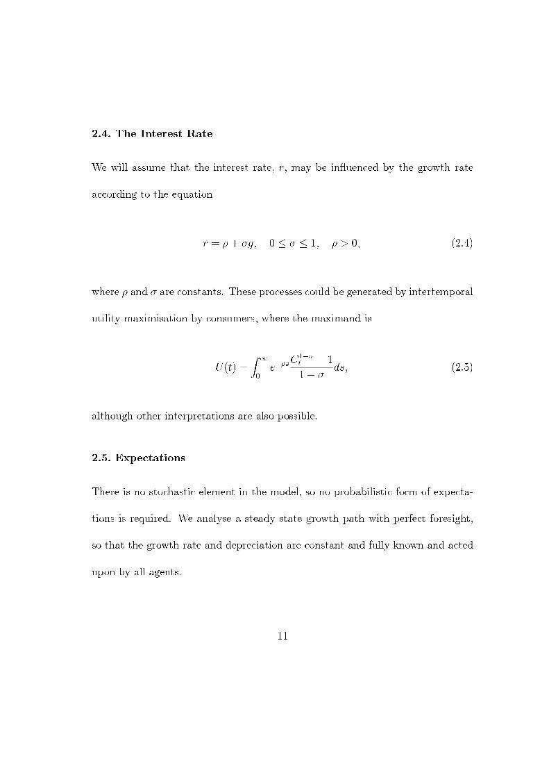
2.4. The Interest Rate

We will assume that the interest rate, r, may be in°uenced by the growth rate

according to the equation

r = ½ + ¾g; 0 · ¾ · 1; ½ > 0; (2.4)

where ½ and ¾ are constants. These processes could be generated by intertemporal

utility maximisation by consumers, where the maximand is

U(t) =Z1

0e¡½s

C1¡¾t ¡ 1

1¡ ¾ds; (2.5)

although other interpretations are also possible.

2.5. Expectations

There is no stochastic element in the model, so no probabilistic form of expecta-

tions is required. We analyse a steady state growth path with perfect foresight,

so that the growth rate and depreciation are constant and fully known and acted

upon by all agents.

11

3. Solving the Steady State

3.1. Machinery

Since physical depreciation is being ignored a priori for simplicity, all depreciation

is a reduction in the value of capital, arising from economic events elsewhere in

the economy. In a model with only a representative good, this is represented

entirely by the increase in the wage paid to labour3, which squeezes the gross

pro¯ts earned by the owner of the machine.

Eventually the wage will rise to the point at which machines of a given vintage

will be retired from production. We will refer to the age of the knowledge em-

bodied in these machines as the retirement age, R. If machines always embodied

the latest knowledge when they were produced, then the machines would also

be R old when they were retired. We will, however, wish to allow the possibil-

ity that machines are produced which do not embody state-of-the-art knowledge.

These machines will still be retired from production when the knowledge that

they embody is R old, although the machines themselves will be younger.

3In an economy with many goods, capital could obsolesce for reasons other than wage in-

creases, such as a fall in the demand for a good arising from cheaper substitutes. It is also

possible that the value of some capital could rise, if technological advances made complements

cheaper, but this would require horizontal di®erentiation.

12

We assume that ¯nal output is produced by perfectly competitive ¯rms and

that there are no economies of scale to either the ¯rm or the industry as a whole.

Thus the number and size of the ¯rms is irrelevant so long as there are su±ciently

many to maintain perfect competition. Because the industry is perfectly compet-

itive, the output of a ¯rm will be absorbed entirely by the inputs. The machine is

paid for at the beginning of its life, the worker on a period by period basis. The

machine will be retired at the point when the wage of machine operators, w (t),

just equals the output generated by the machine. From the de¯nition of R, this

output will be the output generated by a machine R units of time ago, which we

will denote y (t¡R). Hence the wage is de¯ned in terms of the retirement age

w(t) = y(t¡R): (3.1)

The amount that a ¯rm is prepared to pay for the machine will be the present

value of the °ow of output over and above wages, gross pro¯ts. Gross pro¯ts will

depend upon how much the wage lags behind the output of a machine. Let a

denote how long the knowledge embodied in a machine has been available: a is

the age of the knowledge (but not necessarily of the machine). A machine which

embodies knowledge which is a old produces a constant °ow of output y(t ¡ a)

13

and the ¯rm has to pay a wage w(t), which is rising over time, so the gross pro¯ts

generated by the machine is

¼m(t; a) = y(t¡ a)¡ w(t); (3.2)

so long as y(t¡a) ¸ w(t); otherwise the machine would be retired from production.

When both the retirement age and the growth of productivity of machinery are

constant, which they will be in the steady state, then y (t¡R) = y (t) e¡gR, so,

using equation (3.1), we can write the machine's output as

y (t¡ a) = w (t) eg(R¡a): (3.3)

The present value of the pro¯t stream of a machine which embodies technology

of age a is

V (t; a) =Z R¡a

0e¡rs¼m (t+ s; a+ s) ds; (3.4)

which, after appropriate substitution is

V (t; a) = w (t)Z R¡a

0e(g(1¡¾)¡½)s

neg(R¡a¡s) ¡ 1

ods ´ w (t) »(R¡a; g; ½; ¾): (3.5)

14

We introduce the notation » because the solution to the integral is insu±ciently

tractable to allow an analytic solution to the model. We can, however, show that »

is zero when a = R (since that is the point when the machine is obsolete) or g = 0,

in which case gross pro¯ts are zero because the wage does not lag behind machine

productivity. Except in these cases, it is an increasing and convex function of both

the retirement age and the growth rate and a decreasing function of ½4. These

results are intuitive: the longer a machine will be in operation, the more pro¯t

it will generate; the faster the growth rate, the more wages lag behind output;

the higher the value of ½, the higher the interest rate and the more pro¯ts are

discounted.

A ¯rm producing ¯nal output will be prepared to pay up to V for a machine.

Notice that this is not the user cost of capital, which is a °ow concept, but

corresponds more closely to the list price of a machine or the prices implied by

the price de°ator for Gross Domestic Fixed Capital Formation in the national

accounts5.

4Note that gross pro¯ts are zero at R¡a, so by Leibniz's rule we do not need to worry about

changes in the upper limit to the integral. The integrand is clearly an increasing and convex

function of R; these properties follow for g also because 1¡ ¾ and R¡ a¡ s are both (weakly)

positive, by assumption and de¯nition respectively.5A problem remains in that we have normalised the capital to be the amount of capital per

worker: thus to obtain an estimate of V from the national accounts we would also need to take

account of the number of workers expected to use the additional capital created, and the hours

15

3.2. Machine Production

To produce machines, ¯rms only need workers and the knowledge in the patent.

Given access to the relevant knowledge, the relationship between the number of

workers and the number of machines produced is the same for all vintages, namely

fp (t; a) = ´Á (M (t; a)) ; ´ > 0:

The parameter ´ represents the level of productivity in this sector, fp (t; a) is

the density of machines of vintage a in production at time t and M (t; a) is the

number of corresponding workers. The functional form of the production function

is Á, which displays diminishing returns at some point. Instead the properties of

Á, it will be more convenient to consider the average cost curve of the ¯rm. We

consider three possibilities, as shown in Figure 3.1.

Recall that each vintage of intermediate good is produced by one ¯rm alone,

which controls the legal rights to the particular knowledge which will be embod-

ied in its intermediate goods. The ¯rm does not allow other ¯rms to use that

knowledge and maximises pro¯ts based on its own output. Although the ¯rm has

that they would spend operating it. If we could take these factors, together with changes in g

and R into account, equation (3.5) implies that the price de°ator of capital should move in a

similar fashion to the wage.

16

Figure 3.1: Average Cost Curves

a monopoly over its particular vintage, it has no market power, because all of the

vintages are in competition with each other: no ¯rm can charge a price higher

than the value of its intermediate good because buyers can always substitute into

other vintages at an appropriate price6. Thus the ¯rm faces a perfectly elastic

demand curve whose position is determined by the embodied knowledge of the

intermediate good it is selling. Since the ¯rm also takes the wage as given, out-

6An analogy might be the term structure of interest rates (in its (rational) expectations

hypothesis form), where prices adjust to ensure that bonds of di®erent terms are, in e®ect,

substitutes.

17

put will be determined by price equals marginal cost, subject to price exceeding

average cost. As other innovations occur, the price and hence pro¯t will fall.

If the average cost curve is like the ¯rst example in the diagram, the ¯rm will

continue to produce until the price falls to zero, which will occur when the age

of the knowledge it is using (a) is R old. In the other two cases, production will

cease when the price is positive, implying that the age is less than R: we shall call

the age of the knowledge at the moment when it stops being used Q. We shall

not consider the ¯rst case in any detail, since the qualitative results, other than

Q = R, are the same as for the other cases.

Suppose that, at time t, a ¯rm is selling intermediate goods incorporating

knowledge whose obsolescence is a. Suppose that the ¯rm pays a wage w (t) to

workers producing intermediate goods. When it produces fp intermediate goods,

its pro¯ts are

w (t) ¼ (t; a) = V (t; a) fp (t; a)¡ w (t)M (t; a) = w (t) fµ»fp ¡Mg : (3.6)

In the steady state, pro¯ts of a ¯rm producing a vintage of a given age, prices

and wages will all be growing at the same rate g; so henceforth we will simplify

notation by ignoring the dependence of variables on t unless confusion may arise.

18

It follows from the properties of Á, that, so long as the ¯rm is producing at

all, its optimal output, f¤p (a), optimal labour input, M¤ (a), and resulting pro¯t,

¼¤ (a), have the following properties:

@f¤p (a)

@´> 0;

@f ¤p (a)

@»> 0;

@M ¤ (a)

@´> 0;

@M ¤ (a)

@»> 0:

@¼¤

@»> 0;

@¼¤

@´> 0: (3.7)

This result is intuitive: the higher the ratio of the price of machinery to the wage,

the more is produced. Since the ¯rm ceases production only when pro¯ts are zero,

we can formally de¯ne Q by

¼¤ (» (R¡Q; :::) ; ´) = 0: (3.8)

The present value of a ¯rm's pro¯ts when the ¯rm is just set up is

W (t) =Z Q

0w (t+ a)¼¤ (t+ a; a) e¡rada: (3.9)

19

The remuneration from doing research is the value of each innovation multiplied by

the rate at which researchers discover innovations, which we know from equation

(2.3). For workers to be indi®erent between research and producing intermedi-

ate goods, the remuneration from research must equal the wage. Substituting

fg=á1 (g)gW (t) = w (t), we obtain the arbitrage condition

1 =g

á1 (g=À)

Z Q

0e(g(1¡¾)¡½)a¼¤ (» (R ¡ a; g;½;¾) ; ´) da: (3.10)

R is the age at which knowledge embodied in the intermediate good stops being

used, in contrast to Q, the age of knowledge when intermediate goods of that

vintage are no longer produced.

3.3. The Indi®erence Condition

We simplify notation by rewriting equation (3.10) as

1 = £ (R; g; ½; ¾; ´; À) : (3.11)

the complicated nature of » means that there is no useful analytical solution to

the integral, even if we specify Á.

20

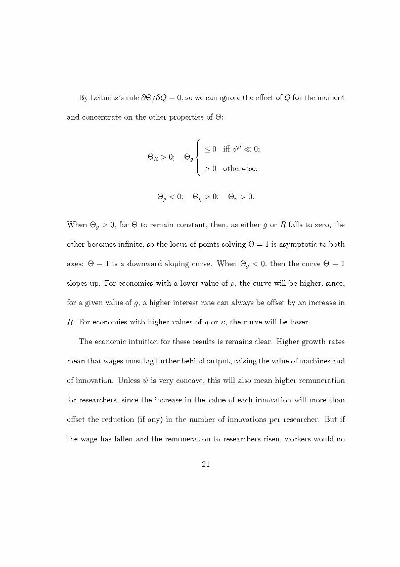
By Leibnitz's rule @£=@Q = 0, so we can ignore the e®ect of Q for the moment

and concentrate on the other properties of £:

£R > 0; £g

8>>><>>>:· 0 i® Ã00 ¿ 0;

> 0 otherwise.

£½ < 0; £´ > 0; £À > 0:

When £g > 0, for £ to remain constant, then, as either g or R falls to zero, the

other becomes in¯nite, so the locus of points solving £ = 1 is asymptotic to both

axes: £ = 1 is a downward sloping curve. When £g < 0, then the curve £ = 1

slopes up. For economies with a lower value of ½, the curve will be higher, since,

for a given value of g, a higher interest rate can always be o®set by an increase in

R. For economies with higher values of ´ or À, the curve will be lower.

The economic intuition for these results is remains clear. Higher growth rates

mean that wages must lag further behind output, raising the value of machines and

of innovation. Unless à is very concave, this will also mean higher remuneration

for researchers, since the increase in the value of each innovation will more than

o®set the reduction (if any) in the number of innovations per researcher. But if

the wage has fallen and the remuneration to researchers risen, workers would no

21

longer be indi®erent between occupations, so it is necessary for some o®-setting

factor to ensure that wages do not fall, namely that the retirement age fall.

If ½ and hence the interest rate is lower, the value of innovation is higher.

When intermediate goods are non-durable, this happens because production is in

the future and the resulting pro¯ts discounted less; when they are durable, not

only are pro¯ts discounted less, but they also rise because machines are more

valuable. If ´ is higher, intermediate good production is cheaper and pro¯ts

and the value of innovation rise. If À increases, then each researcher ¯nds more

innovations. In any of these cases, for a given growth rate, the retirement age must

be lower to ensure that wages do not fall behind the remuneration to research.

3.4. Labour Market Clearing

The model is closed by the labour market clearing condition in equation (2.1). The

number of researchers is known from equation (2.2). The total number of workers

producing intermediate goods is the integral of the number of workers producing

intermediate goods in each vintage, weighted by the density of vintages, which is

M =Z Q

0gM¤ (a) da: (3.12)

22

We know that M¤ (a) is an increasing function of » and hence M is an increasing

function ofR, g and ´ and a decreasing function of ½; by Leibnitz's rule, @M=@Q =

gM ¤ (Q) ¸ 0, where the equality only holds when the cost curve is always upward

sloping.

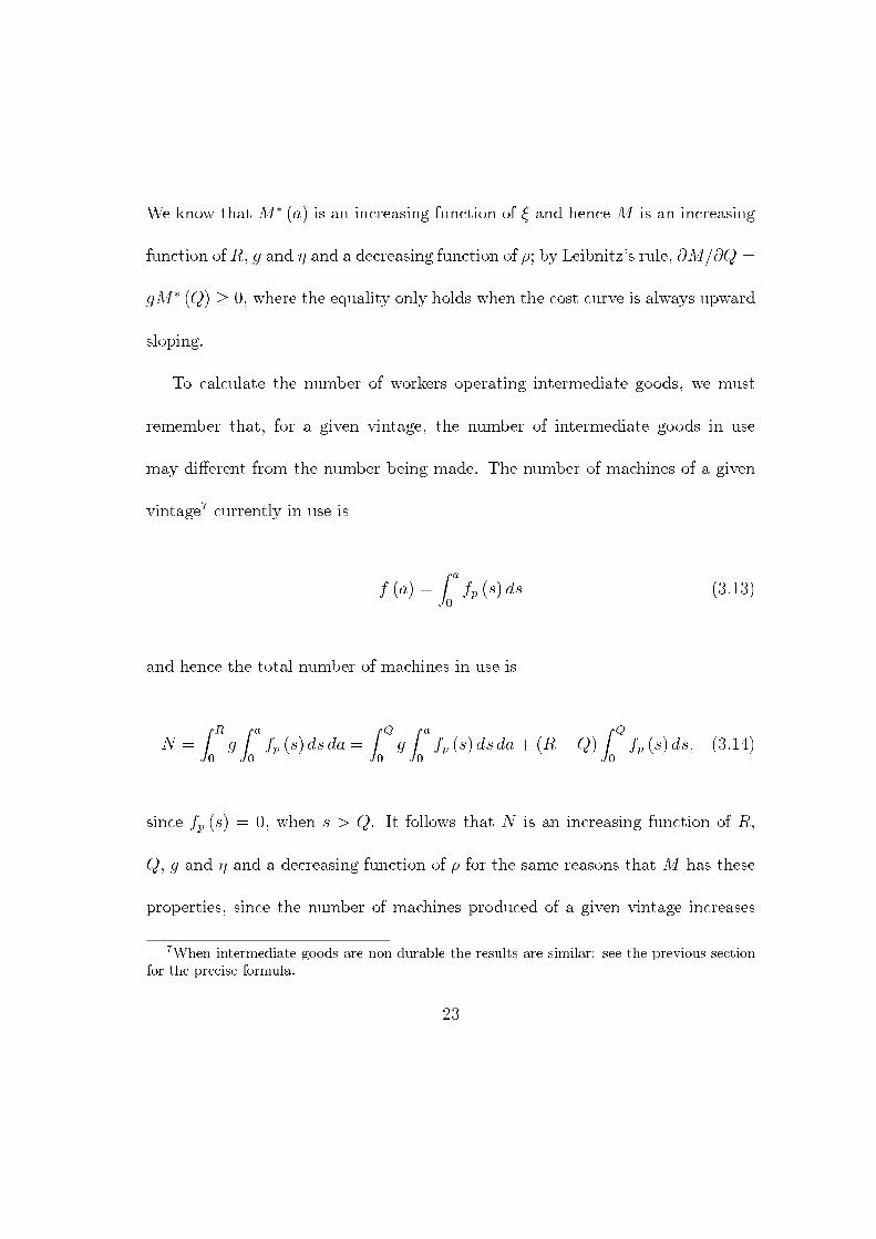
To calculate the number of workers operating intermediate goods, we must

remember that, for a given vintage, the number of intermediate goods in use

may di®erent from the number being made. The number of machines of a given

vintage7 currently in use is

f (a) =Z a

0fp (s) ds (3.13)

and hence the total number of machines in use is

N =Z R

0gZ a

0fp (s) ds da =

Z Q

0gZ a

0fp (s) ds da+ (R¡Q)

Z Q

0fp (s) ds; (3.14)

since fp (s) = 0, when s > Q. It follows that N is an increasing function of R,

Q, g and ´ and a decreasing function of ½ for the same reasons that M has these

properties, since the number of machines produced of a given vintage increases

7When intermediate goods are non-durable the results are similar: see the previous section

for the precise formula.

23

with the number of workers.

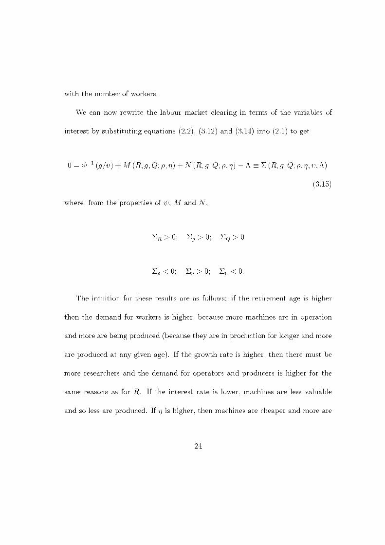
We can now rewrite the labour market clearing in terms of the variables of

interest by substituting equations (2.2), (3.12) and (3.14) into (2.1) to get

0 = á1 (g=À) +M (R;g;Q; ½; ´) +N (R; g;Q; ½; ´)¡ ¤ ´ § (R; g;Q;½; ´; À;¤)

(3.15)

where, from the properties of Ã, M and N ,

§R > 0; §g > 0; §Q > 0

§½ < 0; §´ > 0; §À < 0:

The intuition for these results are as follows: if the retirement age is higher

then the demand for workers is higher, because more machines are in operation

and more are being produced (because they are in production for longer and more

are produced at any given age). If the growth rate is higher, then there must be

more researchers and the demand for operators and producers is higher for the

same reasons as for R. If the interest rate is lower, machines are less valuable

and so less are produced. If ´ is higher, then machines are cheaper and more are

24

produced and operated. If À is lower, more workers are needed to ¯nd the same

number of innovations.

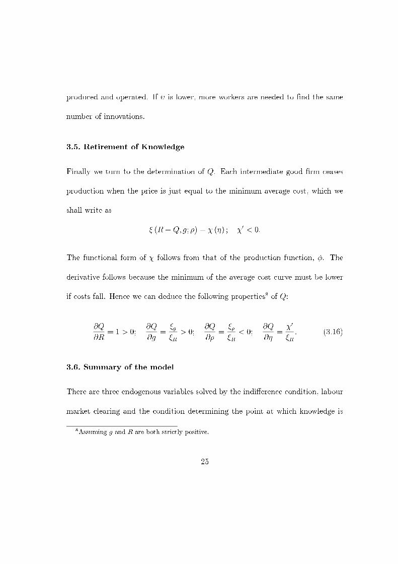
3.5. Retirement of Knowledge

Finally we turn to the determination of Q. Each intermediate good ¯rm ceases

production when the price is just equal to the minimum average cost, which we

shall write as

» (R¡Q;g;½) = Â (´) ; Â0 < 0:

The functional form of  follows from that of the production function, Á. The

derivative follows because the minimum of the average cost curve must be lower

if costs fall. Hence we can deduce the following properties8 of Q:

@Q

@R= 1 > 0;

@Q

@g=

»g

»R> 0;

@Q

@½=

»½

»R< 0;

@Q

@´=

Â0

»R: (3.16)

3.6. Summary of the model

There are three endogenous variables solved by the indi®erence condition, labour

market clearing and the condition determining the point at which knowledge is

8Assuming g and R are both strictly positive.

25

no longer used:

fR; g;Qg :

8>>>>>>>><>>>>>>>>:

1 = £(R; g;Q;p)

0 = § (R; g;Q;p)

0 = » (R ¡Q; g; ½)¡ Â (´) :

where we introduce the notation p, which is a vector of all the parameters of

interest.

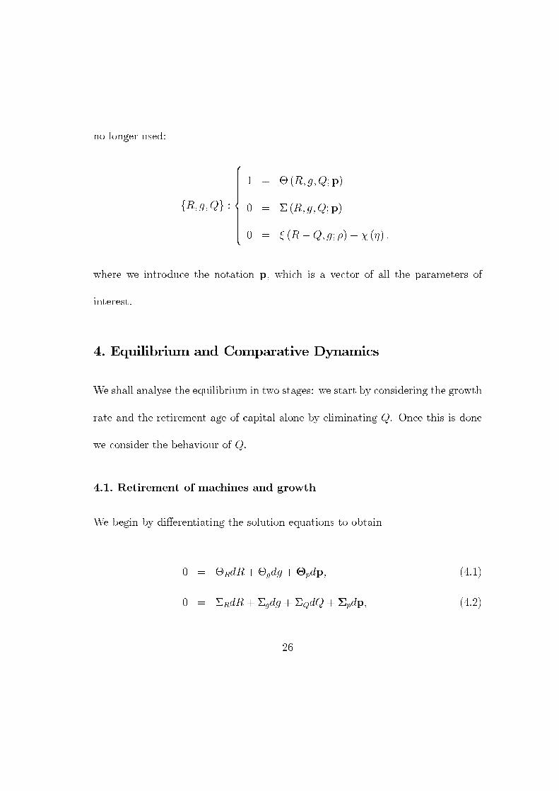
4. Equilibrium and Comparative Dynamics

We shall analyse the equilibrium in two stages: we start by considering the growth

rate and the retirement age of capital alone by eliminating Q. Once this is done

we consider the behaviour of Q.

4.1. Retirement of machines and growth

We begin by di®erentiating the solution equations to obtain

0 = £RdR+£gdg +£pdp; (4.1)

0 = §RdR + §gdg + §QdQ+§pdp; (4.2)

26

0 = »R (dR ¡ dQ) + »gdg +³»p ¡ Âp

´dp: (4.3)

From the third equation we can obtain dQ, and thus eliminate dQ from the

labour market clearing equation, which we rewrite as

0 = §QRdR + §Q

g dg +§Qp dp: (4.4)

It is easy to show that the partial derivatives are qualitatively the same, whether

we have solved for Q or not:

sign§Qi = sign §i i = fR; g;pg

so §Q = 0 will also be a downward sloping curve fg;Rg space and we the analysis

for g and R will be similar regardless of Q.

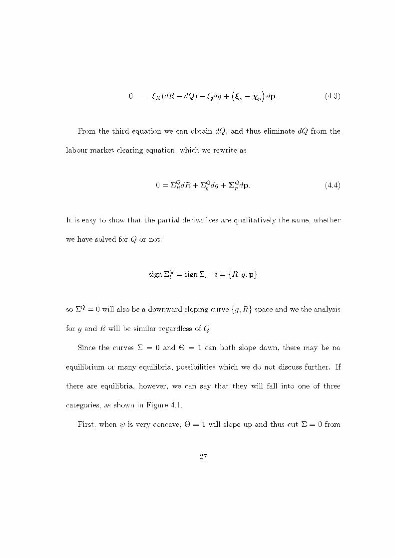
Since the curves § = 0 and £ = 1 can both slope down, there may be no

equilibrium or many equilibria, possibilities which we do not discuss further. If

there are equilibria, however, we can say that they will fall into one of three

categories, as shown in Figure 4.1.

First, when à is very concave, £ = 1 will slope up and thus cut § = 0 from

27

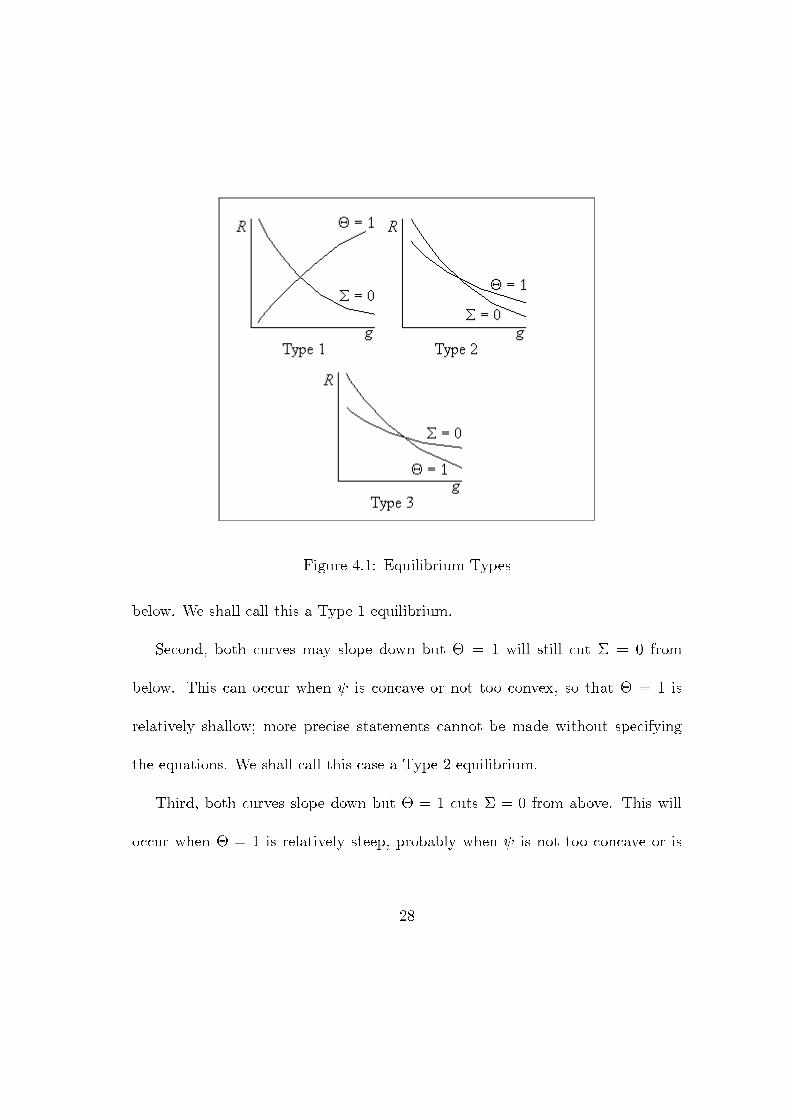
Figure 4.1: Equilibrium Types

below. We shall call this a Type 1 equilibrium.

Second, both curves may slope down but £ = 1 will still cut § = 0 from

below. This can occur when à is concave or not too convex, so that £ = 1 is

relatively shallow; more precise statements cannot be made without specifying

the equations. We shall call this case a Type 2 equilibrium.

Third, both curves slope down but £ = 1 cuts § = 0 from above. This will

occur when £ = 1 is relatively steep, probably when à is not too concave or is

28

convex. This will be a Type 3 equilibrium.

The comparative static properties of the model will depend upon the type of

equilibrium. The derivatives of the two endogenous variables with respect to the

parameters can be obtained by solving equations (4.1) and (4.4):

dg

dp=

§p=§R ¡£p=£R

£g=£R ¡ §g=§R

(4.5)

dR

dp=

(§g=§R) (£p=£R)¡ (£g=£R) (§p=§R)

£g=£R ¡ §g=§R

(4.6)

To discuss the properties of these derivatives for every parameter would be tedious,

so we only consider ¤ and ´ in detail and summarise for the other parameters.

Consider two economies, A and B, where B has a larger labour force. Indif-

ference between occupations is una®ected by the size of the labour force, so both

will have the same £ = 1 curve. The labour market clearing curve for economy

B, however, will be further from the origin, since more workers are available for

either research or investment in machinery, which will lead to higher values of g

or R respectively. The three possibilities are shown in Figure 4.2, with the labour

market clearing conditions labelled \A" and \B" as appropriate. When there is

29

Figure 4.2: Economies with di®erent labour supplies

a Type 1 equilibrium, the growth rate and retirement age will both be higher in

B; when there is a Type 2 equilibrium, the growth rate will be higher and the

retirement age lower; when there is a Type 3 equilibrium, the growth rate will be

lower and the retirement age higher.

The intuition behind these results is fairly straight-forward. More workers are

available in B, so there is the potential for greater research e®ort. But potential

researchers will need to be compensated for two costs. First, if à is concave,

30

there are negative externalities in the research sector, so the greater the number

of researchers the fewer innovations discovered by each individual. Second, if the

growth rate is higher in the future, then potential researchers may anticipate that

newer vintages will displace older ones more quickly. This is \creative destruc-

tion" of machinery, since the increased speed of innovation leads to machinery

being scrapped more quickly (corresponding to a lower retirement age). Creative

destruction of machinery does not directly concern researchers; their remunera-

tion per innovation is the value of the patent. The patent price does, however,

depend upon the value of machinery amongst other things, so researchers are in-

directly a®ected by the creative destruction of machinery. Thus the researchers

in economy B must be compensated for the externalities and their expectations

concerning the e®ect of creative destruction on the value of each patent.

Ceteris Paribus, if the growth rate were expected to be higher in the future,

researchers would expect the value of each patent to be higher, since wages would

lag further behind machine prices making machinery production, and hence inno-

vation, more pro¯table relative to producing or operating machinery. This e®ect

will often su±ce to compensate researchers for any fall in the value of each patent

due to creative destruction and any negative externalities and, anticipating this,

31

more workers will choose to do research. This is a Type 2 equilibrium.

Sometimes, however, the negative externalities and di®erence in the patent

price cannot be compensated by expectations of a higher growth rate, in which

case more workers will choose to do research in economy B only if they expect

there to be less creative destruction (a higher retirement age). This is a Type 1

equilibrium.

Finally, it may be the case that there is no growth rate higher than that in

economy A which will compensate potential researchers in economy B for the

patent price. Anticipating this, workers in B will avoid research and the growth

rate will be lower. But this will also mean that the ratio of machine prices to

wages will also be lower unless there is less creative destruction, so the retirement

age will have to be higher.

We now assume that economies A and B are the same in all respects except

that economy B has a more productive machine producing sector, that is a higher

value of ´. This means that both the curve £ = 1 and the curve § = 0 for economy

B lie below those of economy A. For a Type 1 equilibrium the retirement age will

be lower in B than in A, but the growth rate may either rise or fall. For both

a Type 2 and a Type 3 equilibrium, all that we can say is that it is impossible

32

for both the retirement age and the growth rate to be higher in B than in A; the

retirement age may be higher and the growth rate lower, the retirement age may

be lower and the growth rate higher or both may be higher.

The reason for these ambiguous results is that higher productivity in the ma-

chine will encourage more production and reduce the retirement age. This will

happen even if there is no increase in the growth rate, but it will still reduce the

patent price through creative destruction. On the other hand, higher productivity

will increase the pro¯tability of machine producing ¯rms and mean that the value

of a patent will be higher, encouraging more innovation. Again, this is true even

if there is no di®erence in the growth rate. Thus ¯rms will expect to produce

machines more quickly but for a shorter period of time. Thus the direct produc-

tivity e®ect on patents is ambiguous. On top of this e®ect, however, there is the

two e®ects mentioned in the previous section: any changes in the growth rate will

also a®ect the value of patents and the number of innovations produced by each

researcher.

In Type 2 and Type 3 equilibria, we can exclude the possibility that both

the retirement age and the growth rate will be higher. This would mean that

researchers bene¯ted from higher ´, R and g, all of which would make workers

33

prefer to do research and thus violate the indi®erence condition. In Type 1 equi-

libria, we can also exclude the possibility that the retirement age be higher and

the growth rate lower; because of the large externalities, a lower growth rate would

make researchers better o® and also violate the indi®erence condition.

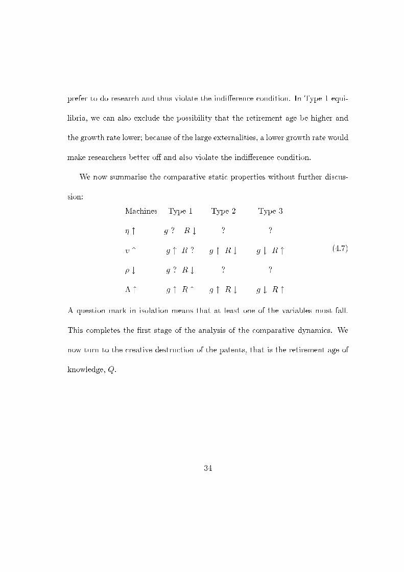
We now summarise the comparative static properties without further discus-

sion:

Machines Type 1 Type 2 Type 3

´ " g ? R # ? ?

À " g " R ? g " R # g # R "

½ # g ? R # ? ?

¤ " g " R " g " R # g # R "

(4.7)

A question mark in isolation means that at least one of the variables must fall.

This completes the ¯rst stage of the analysis of the comparative dynamics. We

now turn to the creative destruction of the patents, that is the retirement age of

knowledge, Q.

34

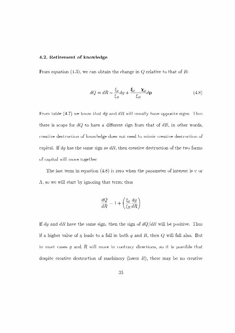
4.2. Retirement of knowledge

From equation (4.3), we can obtain the change in Q relative to that of R:

dQ = dR +»g

»Rdg +

»p ¡ Âp

»Rdp (4.8)

From table (4.7) we know that dg and dR will usually have opposite signs. Thus

there is scope for dQ to have a di®erent sign from that of dR, in other words,

creative destruction of knowledge does not need to mimic creative destruction of

capital. If dg has the same sign as dR, then creative destruction of the two forms

of capital will move together

The last term in equation (4.8) is zero when the parameter of interest is À or

¤, so we will start by ignoring that term; thus

dQ

dR= 1 +

ûg

»R

dg

dR

!

If dg and dR have the same sign, then the sign of dQ=dR will be positive. Thus

if a higher value of ´ leads to a fall in both g and R, then Q will fall also. But

in most cases g and R will move in contrary directions, so it is possible that

despite creative destruction of machinery (lower R), there may be no creative

35

destruction of knowledge and that patents will increase in value. This will happen

when the term in brackets is large (and negative). We cannot, however, evaluate

the bracket without precise knowledge of the functional form, even by a Taylor

expansion around g = 0: the limit of »g=»R as g tends to zero is in¯nite9 and the

limit of dg=dR must be zero as g tends to zero if the indi®erence condition is to

be satis¯ed.

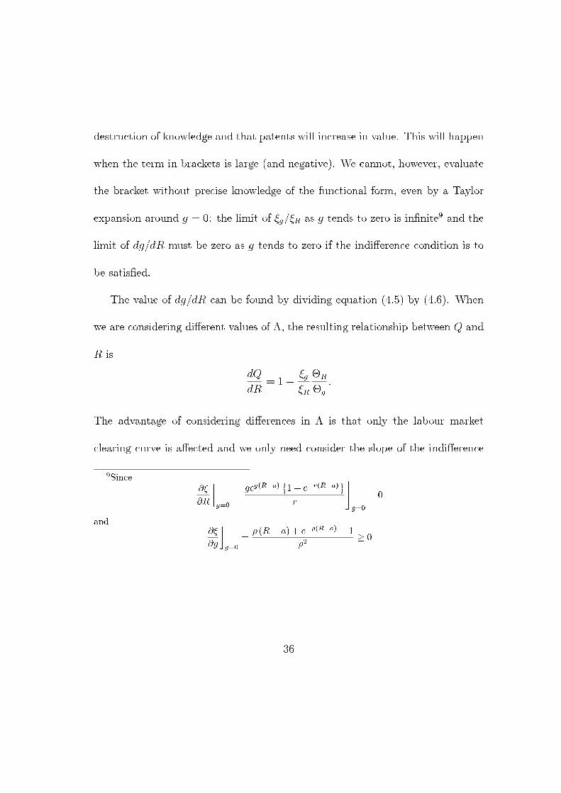
The value of dg=dR can be found by dividing equation (4.5) by (4.6). When

we are considering di®erent values of ¤, the resulting relationship between Q and

R is

dQ

dR= 1 ¡

»g

»R

£R

£g

:

The advantage of considering di®erences in ¤ is that only the labour market

clearing curve is a®ected and we only need consider the slope of the indi®erence

9Since

@»

@R

ºg=0

=geg(R¡a)

©1¡ e¡r(R¡a)

ªr

%g=0

= 0

and@»

@g

ºg=0

=½ (R¡ a) + e¡½(R¡a) ¡ 1

½2¸ 0

36

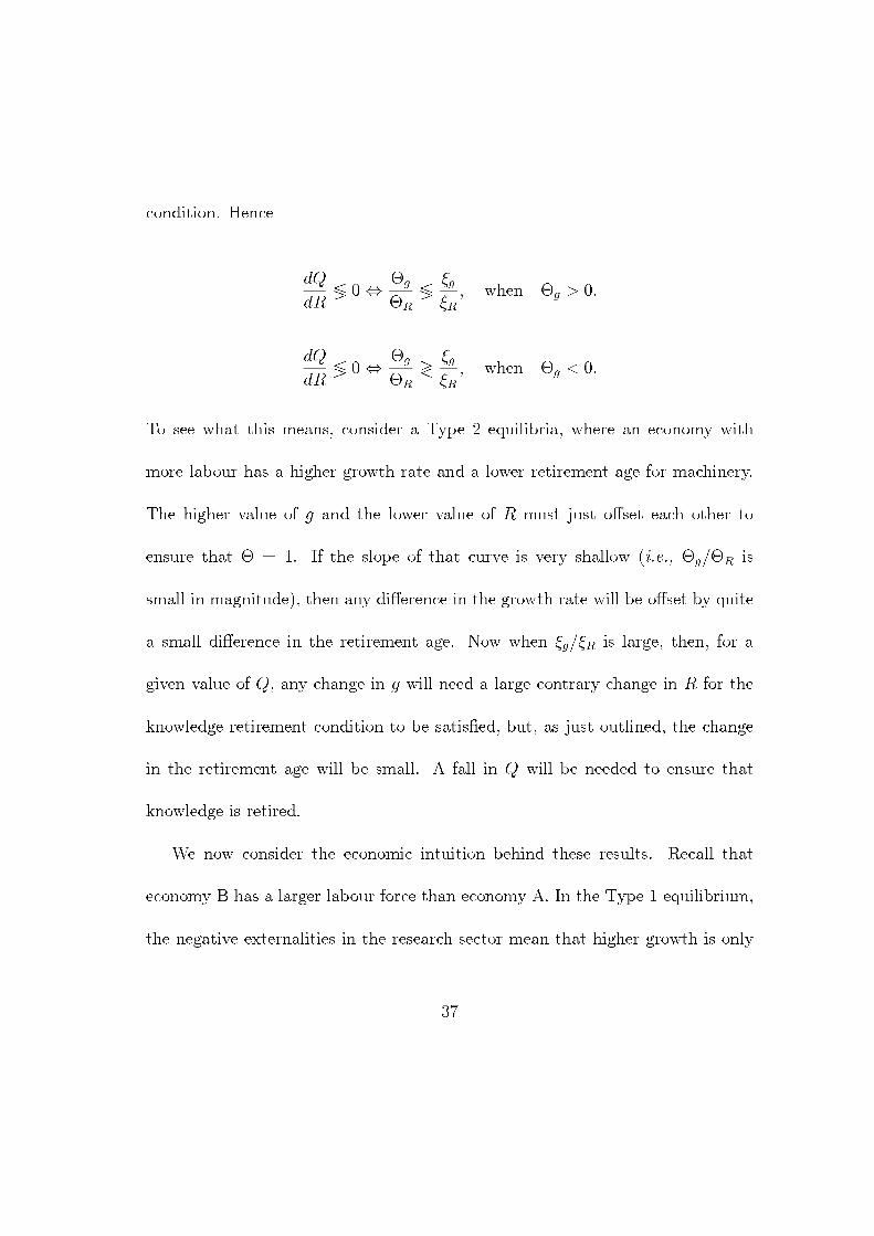
condition. Hence

dQ

dR7 0,

£g

£R

7»g

»R; when £g > 0:

dQ

dR7 0,

£g

£R

?»g

»R; when £g < 0:

To see what this means, consider a Type 2 equilibria, where an economy with

more labour has a higher growth rate and a lower retirement age for machinery.

The higher value of g and the lower value of R must just o®set each other to

ensure that £ = 1. If the slope of that curve is very shallow (i.e., £g=£R is

small in magnitude), then any di®erence in the growth rate will be o®set by quite

a small di®erence in the retirement age. Now when »g=»R is large, then, for a

given value of Q, any change in g will need a large contrary change in R for the

knowledge retirement condition to be satis¯ed, but, as just outlined, the change

in the retirement age will be small. A fall in Q will be needed to ensure that

knowledge is retired.

We now consider the economic intuition behind these results. Recall that

economy B has a larger labour force than economy A. In the Type 1 equilibrium,

the negative externalities in the research sector mean that higher growth is only

37

possible if workers anticipate less depreciation. There is no prima facie reason

why they should require less depreciation of both machinery and knowledge, but

the theory indicates that this is the case: £g=£R; which is negative, cannot be

greater than »g=»R; which is positive.

In the Type 2 equilibrium, a higher growth rate means that each researcher

is making more discoveries and to keep workers indi®erent between research and

other occupations this is compensated by greater creative destruction. This will

always be achieved by greater creative destruction of machinery, but will only

sometimes be achieved by additional creative destruction of knowledge. The latter

will be unnecessary when the creative destruction of machinery has a relatively

large e®ect on the patent price compared to the e®ect on the knowledge retirement

price.

Finally, when workers are discouraged from research by their anticipation that

the value of patents will be quickly undermined by future research, there will

be less creative destruction of machinery, which will only sometimes need to be

accompanied by less creative destruction of knowledge.

The e®ects of higher values of ¤ are summarised in Figure 4.3. It is assumed

that there is some measure of convexity of à which can be plotted on the hori-

38

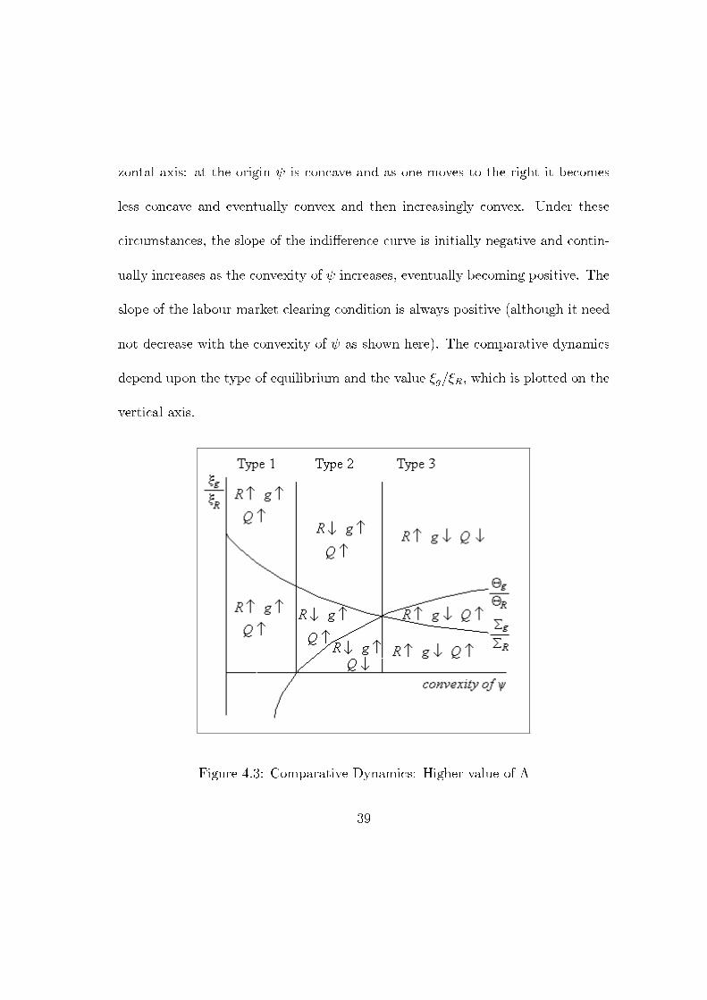
zontal axis: at the origin à is concave and as one moves to the right it becomes

less concave and eventually convex and then increasingly convex. Under these

circumstances, the slope of the indi®erence curve is initially negative and contin-

ually increases as the convexity of à increases, eventually becoming positive. The

slope of the labour market clearing condition is always positive (although it need

not decrease with the convexity of à as shown here). The comparative dynamics

depend upon the type of equilibrium and the value »g=»R, which is plotted on the

vertical axis.

Figure 4.3: Comparative Dynamics: Higher value of ¤

39

Similar results can be obtained for the other parameters.

5. Local Stability

Faced with this range of comparative static properties it is reasonable to ask if

any of them can be excluded for any reason. Here we consider local stability,

when expectations are that the economy will remain in the steady state. From

a position of equilibrium, we consider the forces acting on the economy when it

moves a little way from equilibrium, but expectations do not change

First of all, consider the condition that workers be indi®erent between research

and either producing or operating intermediate goods. In the steady state this is

determined by

£ (R¤; g¤; r) = 1:

We know that the e®ect on £ of a small increase in R is positive. The e®ect on £

of a small increase in g (t) is negligible. The reason that g enters as an argument

of £ is that, in the steady state, it determines the rate at which wages increase

and hence the pro¯tability of intermediate good and, in turn, the pro¯tability of

producing intermediate good. Out of the steady state, the rate at which wages

increase will depend upon the rate at which productivity was increasing when

40