Cricket analytics with cricketr

Tinniam V Ganesh

tvganesh.85@gmail.com

Preface Cricket has been the “national passion” of India for decades. As a boy I was also held in thrall by a strong cricketing

passion like many. Cricket is a truly fascinating game! I would catch the sporting action with my friends as we crowded around a transistor that brought us live, breathless radio commentary. We also spent many hours glued to live cricket

action on the early black and white TVs. This used to be an experience of sorts, as every now and then a part of the

body of the players, would detach itself and stretch to the sides. But it was enjoyable all the same.

Nowadays broadcast technology has improved so much and we get detailed visual analysis of the how each bowler

varies the swing and length of the delivery. We are also able to see the strokes of batsman in slow motion. Similarly

computing technology has also advanced by leaps and bounds and we can analyze players in great detail with a few lines of code in languages like R, Python etc.

In 2015, I completed Machine Learning from Stanford at Coursera. I was looking around for data to play around with, when it suddenly struck me that I could do some regression analysis of batting records. In the subsequent months, I

took the Data Science Specialization from John Hopkins University, which triggered more ideas in me. One thing led to

another and I managed to put together an R package called ‘cricketr’. I developed this package over 7 months adding and refining functions. Finally, I managed to submit the package to CRAN. During the development of the package for

different formats of the game I wrote a series of posts in my blog.

This book is a collection of those cricket related posts. There are 6 posts based on my R package cricketr. I have also included 2 earlier posts based on R which I wrote before I created my R package. Finally, I also include another 2

cricket posts based on Machine Learning in which I used the language Octave.

My cricketr’ package is a first, for cricket analytics, howzat! and I am certain that it won’t be the last. Cricket is a

wonderful pitch for statisticians, data scientists and machine learning experts. So you can expect some cool packages in

the years to come.

I had a great time developing the package. I hope you have a wonderful time reading this book.

Feel free to get in touch with me anytime through email included below

Tinniam V Ganesh tvganesh.85@gmail.com

January 28, 2016

Cricket Analytics with cricketr

1.1. Introducing cricketr! : An R package to analyze performances

of cricketers

Yet all experience is an arch wherethro’

Gleams that untravell’d world whose margin fades

For ever and forever when I move.

How dull it is to pause, to make an end,

To rust unburnish’d, not to shine in use!

Ulysses by Alfred Tennyson

1.1.1. Introduction

This is an initial post in which I introduce a cricketing package ‘cricketr’ which I have created. This package was a

natural culmination to my earlier posts on cricket and my finishing 10 modules of Data Science Specialization, from

John Hopkins University at Coursera. The thought of creating this package struck me some time back, and I have finally been able to bring this to fruition.

So here it is. My R package ‘cricketr!!!’

This package uses the statistics info available in ESPN Cricinfo Statsguru. The current version of this package can

handle all formats of the game including Test, ODI and Twenty20 cricket.

You should be able to install the package from GitHub and use many of the functions available in the package. Please

be mindful of ESPN Cricinfo Terms of Use

(Note: This page is also hosted as a GitHub page at cricketr and also at RPubs ascricketr: A R package for analyzing

performances of cricketers

You can download this analysis as a PDF file from Introducing cricketr

(R package cricketr Take a look at my short video tutorial on my on Youtube – R package cricketr – A short tutorial)

Do check out my interactive Shiny app implementation using the cricketr package –Sixer – R package cricketr’s new Shiny

avatar

1.1.2. The cricketr package

The cricketr package has several functions that perform several different analyses on both batsman and bowlers. The

package has functions that plot percentage frequency runs or wickets, runs likelihood for a batsman, relative run/strike

rates of batsman and relative performance/economy rate for bowlers are available.

Other interesting functions include batting performance moving average, forecast and a function to check whether the

batsman/bowler is in in-form or out-of-form.

The data for a particular player can be obtained with the getPlayerData() function from the package. To do this you will

need to go to ESPN CricInfo Player and type in the name of the player for e.g Ricky Ponting, Sachin Tendulkar etc.

This will bring up a page which have the profile number for the player e.g. for Sachin Tendulkar this would

be http://www.espncricinfo.com/india/content/player/35320.html. Hence, Sachin’s profile is 35320. This can be used to

get the data for Tendulkar as shown below

The cricketr package is now available from CRAN!!!. You should be able to install directly with if (!require("cricketr")){ install.packages("cricketr",lib = "c:/test") } library(cricketr)

The cricketr package includes some pre-packaged sample (.csv) files. You can use these sample to test functions as

shown below

# Retrieve the file path of a data file installed with cricketr pathToFile <- system.file("data", "tendulkar.csv", package = "cricketr") batsman4s(pathToFile, "Sachin Tendulkar")

# The general format is pkg-function(pathToFile,par1,...) batsman4s(<path-To-File>,"Sachin Tendulkar")

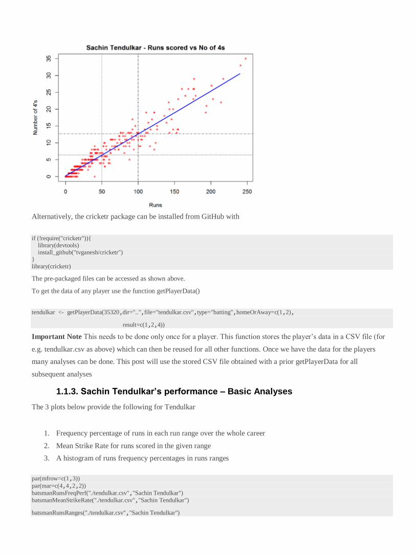
Alternatively, the cricketr package can be installed from GitHub with

if (!require("cricketr")){ library(devtools) install_github("tvganesh/cricketr") } library(cricketr)

The pre-packaged files can be accessed as shown above.

To get the data of any player use the function getPlayerData()

tendulkar <- getPlayerData(35320,dir="..",file="tendulkar.csv",type="batting",homeOrAway=c(1,2),

result=c(1,2,4))

Important Note This needs to be done only once for a player. This function stores the player’s data in a CSV file (for

e.g. tendulkar.csv as above) which can then be reused for all other functions. Once we have the data for the players

many analyses can be done. This post will use the stored CSV file obtained with a prior getPlayerData for all

subsequent analyses

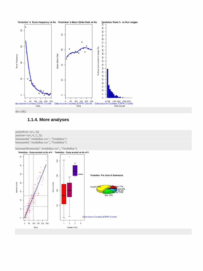
1.1.3. Sachin Tendulkar’s performance – Basic Analyses

The 3 plots below provide the following for Tendulkar

1. Frequency percentage of runs in each run range over the whole career

2. Mean Strike Rate for runs scored in the given range

3. A histogram of runs frequency percentages in runs ranges

par(mfrow=c(1,3)) par(mar=c(4,4,2,2)) batsmanRunsFreqPerf("./tendulkar.csv","Sachin Tendulkar") batsmanMeanStrikeRate("./tendulkar.csv","Sachin Tendulkar")

batsmanRunsRanges("./tendulkar.csv","Sachin Tendulkar")

dev.off()

1.1.4. More analyses

par(mfrow=c(1,3)) par(mar=c(4,4,2,2)) batsman4s("./tendulkar.csv","Tendulkar") batsman6s("./tendulkar.csv","Tendulkar")

batsmanDismissals("./tendulkar.csv","Tendulkar")

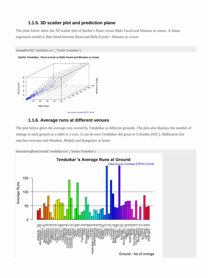
1.1.5. 3D scatter plot and prediction plane

The plots below show the 3D scatter plot of Sachin’s Runs versus Balls Faced and Minutes at crease. A linear

regression model is then fitted between Runs and Balls Faced + Minutes at crease

battingPerf3d("./tendulkar.csv","Sachin Tendulkar")

1.1.6. Average runs at different venues

The plot below gives the average runs scored by Tendulkar at different grounds. The plot also displays the number of

innings at each ground as a label at x-axis. It can be seen Tendulkar did great in Colombo (SSC), Melbourne ifor

matches overseas and Mumbai, Mohali and Bangalore at home

batsmanAvgRunsGround("./tendulkar.csv","Sachin Tendulkar")

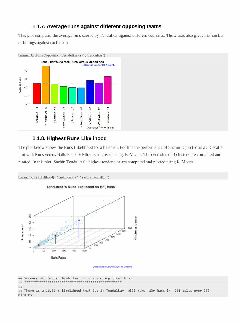
1.1.7. Average runs against different opposing teams

This plot computes the average runs scored by Tendulkar against different countries. The x-axis also gives the number

of innings against each team

batsmanAvgRunsOpposition("./tendulkar.csv","Tendulkar")

1.1.8. Highest Runs Likelihood

The plot below shows the Runs Likelihood for a batsman. For this the performance of Sachin is plotted as a 3D scatter

plot with Runs versus Balls Faced + Minutes at crease using. K-Means. The centroids of 3 clusters are computed and

plotted. In this plot. Sachin Tendulkar’s highest tendencies are computed and plotted using K-Means

batsmanRunsLikelihood("./tendulkar.csv","Sachin Tendulkar")

## Summary of Sachin Tendulkar 's runs scoring likelihood ## ************************************************** ## ## There is a 16.51 % likelihood that Sachin Tendulkar will make 139 Runs in 251 balls over 353 Minutes

## There is a 58.41 % likelihood that Sachin Tendulkar will make 16 Runs in 31 balls over 44 Minutes

## There is a 25.08 % likelihood that Sachin Tendulkar will make 66 Runs in 122 balls over 167 Minutes

1.1.9. A look at the Top 4 batsman – Tendulkar, Kallis, Ponting and Sangakkara

The batsmen with the most hundreds in test cricket are

1. Sachin Tendulkar :Average:53.78,100’s – 51, 50’s – 68

2. Jacques Kallis : Average: 55.47, 100’s – 45, 50’s – 58

3. Ricky Ponting : Average: 51.85, 100’s – 41 , 50’s – 62

4. Kumara Sangakarra: Average: 58.04 ,100’s – 38 , 50’s – 52

in that order.

The following plots take a closer at their performances. The box plots show the mean (red line) and median (blue line).

The two ends of the boxplot display the 25th and 75th percentile.

1.1.10. Performance at home and overseas

From the plot below it can be seen

Tendulkar has more matches overseas than at home and his performance is consistent in all venues at home or abroad.

Ponting has lesser innings than Tendulkar and has an equally good performance at home and overseas.Kallis and

Sangakkara’s performance abroad is lower than the performance at home.

This function also requires the use of getPlayerDataSp() as shown above

par(mfrow=c(2,2)) par(mar=c(4,4,2,2)) batsmanPerfHomeAway("tendulkarsp.csv","Tendulkar") batsmanPerfHomeAway("kallissp.csv","Kallis") batsmanPerfHomeAway("pontingsp.csv","Ponting") batsmanPerfHomeAway("sangakkarasp.csv","Sangakarra") dev.off()

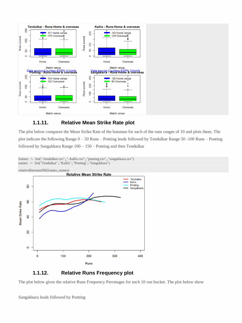
1.1.11. Relative Mean Strike Rate plot

The plot below compares the Mean Strike Rate of the batsman for each of the runs ranges of 10 and plots them. The

plot indicate the following Range 0 – 50 Runs – Ponting leads followed by Tendulkar Range 50 -100 Runs – Ponting

followed by Sangakkara Range 100 – 150 – Ponting and then Tendulkar

frames <- list("./tendulkar.csv","./kallis.csv","ponting.csv","sangakkara.csv") names <- list("Tendulkar","Kallis","Ponting","Sangakkara")

relativeBatsmanSR(frames,names)

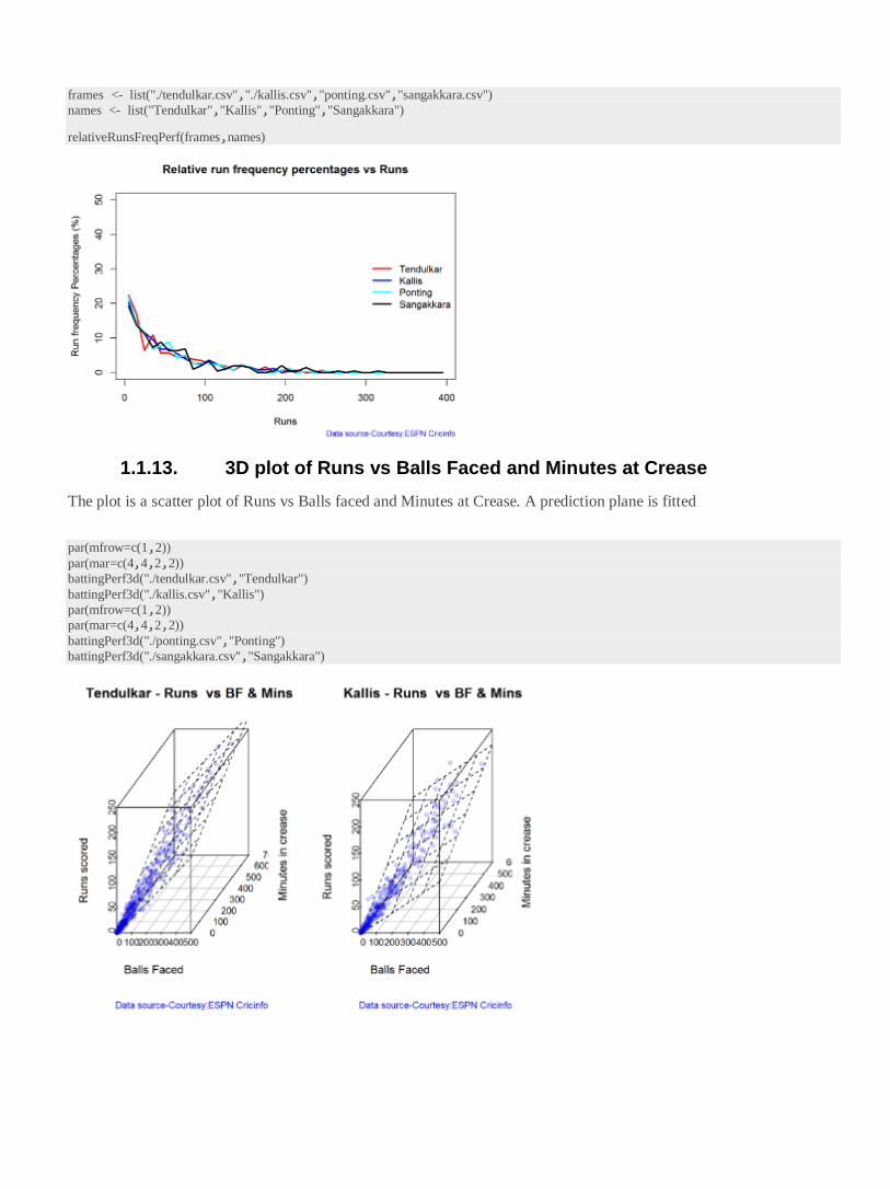
1.1.12. Relative Runs Frequency plot

The plot below gives the relative Runs Frequency Percetages for each 10 run bucket. The plot below show

Sangakkara leads followed by Ponting

frames <- list("./tendulkar.csv","./kallis.csv","ponting.csv","sangakkara.csv") names <- list("Tendulkar","Kallis","Ponting","Sangakkara")

relativeRunsFreqPerf(frames,names)

1.1.13. 3D plot of Runs vs Balls Faced and Minutes at Crease

The plot is a scatter plot of Runs vs Balls faced and Minutes at Crease. A prediction plane is fitted

par(mfrow=c(1,2)) par(mar=c(4,4,2,2)) battingPerf3d("./tendulkar.csv","Tendulkar")

battingPerf3d("./kallis.csv","Kallis")

par(mfrow=c(1,2)) par(mar=c(4,4,2,2)) battingPerf3d("./ponting.csv","Ponting") battingPerf3d("./sangakkara.csv","Sangakkara")

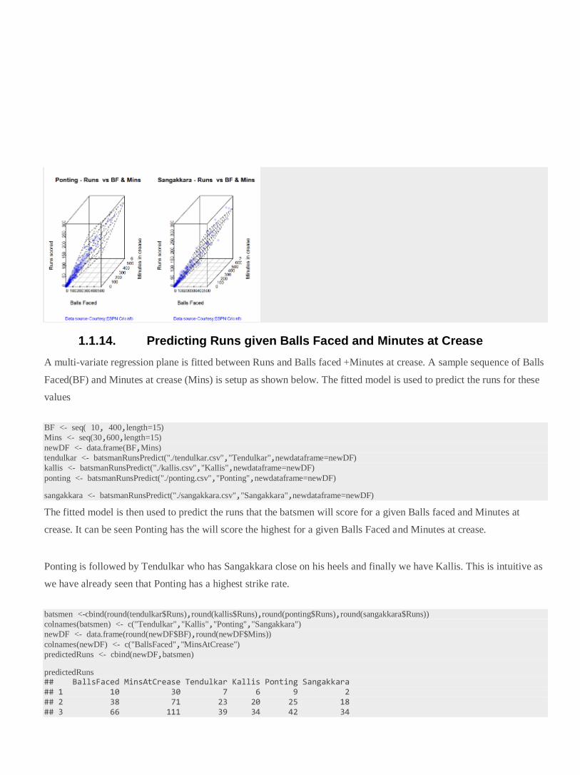
1.1.14. Predicting Runs given Balls Faced and Minutes at Crease

A multi-variate regression plane is fitted between Runs and Balls faced +Minutes at crease. A sample sequence of Balls

Faced(BF) and Minutes at crease (Mins) is setup as shown below. The fitted model is used to predict the runs for these

values

BF <- seq( 10, 400,length=15) Mins <- seq(30,600,length=15) newDF <- data.frame(BF,Mins) tendulkar <- batsmanRunsPredict("./tendulkar.csv","Tendulkar",newdataframe=newDF) kallis <- batsmanRunsPredict("./kallis.csv","Kallis",newdataframe=newDF) ponting <- batsmanRunsPredict("./ponting.csv","Ponting",newdataframe=newDF)

sangakkara <- batsmanRunsPredict("./sangakkara.csv","Sangakkara",newdataframe=newDF)

The fitted model is then used to predict the runs that the batsmen will score for a given Balls faced and Minutes at

crease. It can be seen Ponting has the will score the highest for a given Balls Faced and Minutes at crease.

Ponting is followed by Tendulkar who has Sangakkara close on his heels and finally we have Kallis. This is intuitive as

we have already seen that Ponting has a highest strike rate.

batsmen <-cbind(round(tendulkar$Runs),round(kallis$Runs),round(ponting$Runs),round(sangakkara$Runs)) colnames(batsmen) <- c("Tendulkar","Kallis","Ponting","Sangakkara") newDF <- data.frame(round(newDF$BF),round(newDF$Mins)) colnames(newDF) <- c("BallsFaced","MinsAtCrease") predictedRuns <- cbind(newDF,batsmen)

predictedRuns ## BallsFaced MinsAtCrease Tendulkar Kallis Ponting Sangakkara ## 1 10 30 7 6 9 2 ## 2 38 71 23 20 25 18 ## 3 66 111 39 34 42 34

## 4 94 152 54 48 59 50 ## 5 121 193 70 62 76 66 ## 6 149 234 86 76 93 82 ## 7 177 274 102 90 110 98 ## 8 205 315 118 104 127 114 ## 9 233 356 134 118 144 130 ## 10 261 396 150 132 161 146 ## 11 289 437 165 146 178 162 ## 12 316 478 181 159 194 178 ## 13 344 519 197 173 211 194 ## 14 372 559 213 187 228 210

## 15 400 600 229 201 245 226

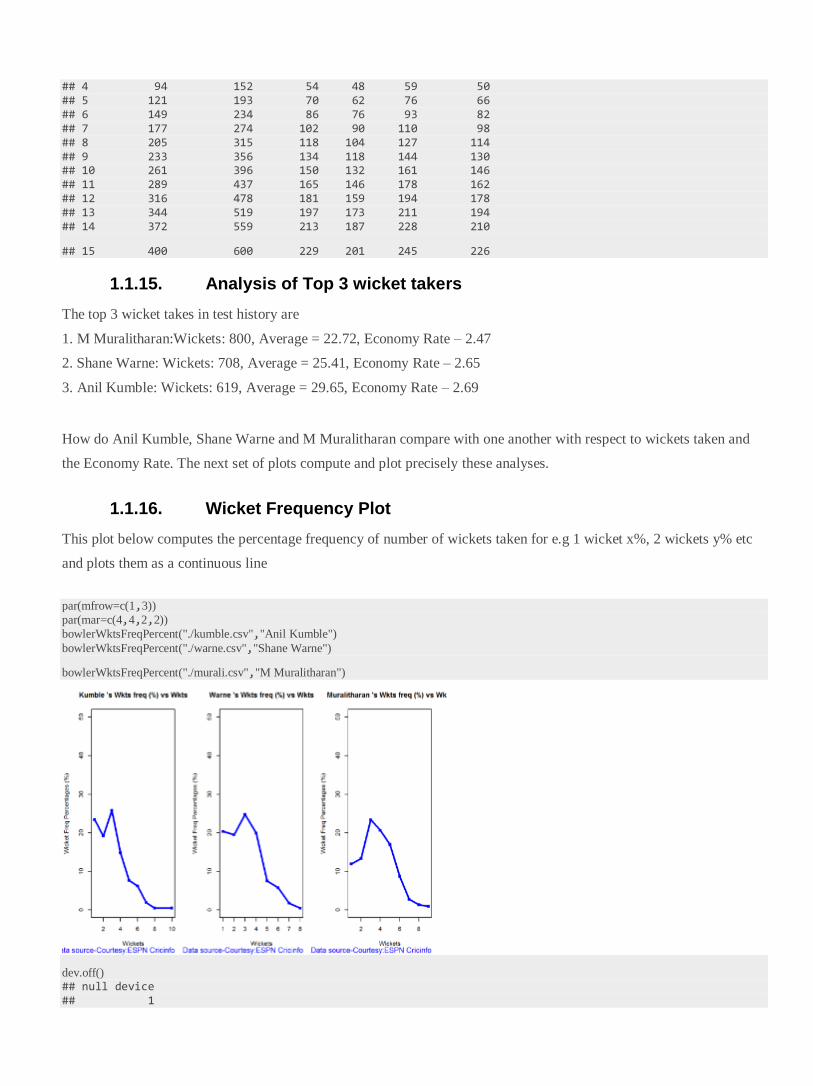
1.1.15. Analysis of Top 3 wicket takers

The top 3 wicket takes in test history are

1. M Muralitharan:Wickets: 800, Average = 22.72, Economy Rate – 2.47

2. Shane Warne: Wickets: 708, Average = 25.41, Economy Rate – 2.65

3. Anil Kumble: Wickets: 619, Average = 29.65, Economy Rate – 2.69

How do Anil Kumble, Shane Warne and M Muralitharan compare with one another with respect to wickets taken and

the Economy Rate. The next set of plots compute and plot precisely these analyses.

1.1.16. Wicket Frequency Plot

This plot below computes the percentage frequency of number of wickets taken for e.g 1 wicket x%, 2 wickets y% etc

and plots them as a continuous line

par(mfrow=c(1,3)) par(mar=c(4,4,2,2)) bowlerWktsFreqPercent("./kumble.csv","Anil Kumble") bowlerWktsFreqPercent("./warne.csv","Shane Warne")

bowlerWktsFreqPercent("./murali.csv","M Muralitharan")

dev.off() ## null device ## 1

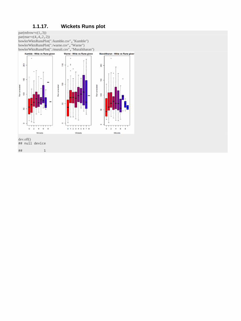
1.1.17. Wickets Runs plot par(mfrow=c(1,3)) par(mar=c(4,4,2,2)) bowlerWktsRunsPlot("./kumble.csv","Kumble") bowlerWktsRunsPlot("./warne.csv","Warne") bowlerWktsRunsPlot("./murali.csv","Muralitharan")

dev.off() ## null device

## 1

1.2. cricketr plays the ODIs!

1.2.1. Introduction

In this post my package ‘cricketr’ takes a swing at One Day Internationals(ODIs). Like test batsman who adapt to ODIs

with some innovative strokes, the cricketr package has some additional functions and some modified functions to

handle the high strike and economy rates in ODIs. As before I have chosen my top 4 ODI batsmen and top 4 ODI

bowlers.

Do check out my interactive Shiny app implementation using the cricketr package –Sixer – R package cricketr’s new

Shiny avatar

You can also read this post at Rpubs as odi-cricketr. Dowload this report as a PDF file from odi-cricketr.pdf

Batsmen

4. Virendar Sehwag (Ind)

5. AB Devilliers (SA)

6. Chris Gayle (WI)

7. Glenn Maxwell (Aus)

Bowlers

5. Mitchell Johnson (Aus)

6. Lasith Malinga (SL)

7. Dale Steyn (SA)

8. Tim Southee (NZ)

I have sprinkled the plots with a few of my comments. Feel free to draw your conclusions! The analysis is included

below

The profile for Virender Sehwag is 35263. This can be used to get the ODI data for Sehwag. For a batsman the type

should be “batting” and for a bowler the type should be “bowling” and the function is getPlayerDataOD()

The package can be installed directly from CRAN

if (!require("cricketr")){ install.packages("cricketr",lib = "c:/test") }

library(cricketr)

or from Github

library(devtools) install_github("tvganesh/cricketr") library(cricketr)

The One day data for a particular player can be obtained with the getPlayerDataOD() function. To do you will need to

go to ESPN CricInfo Player and type in the name of the player for e.g Virendar Sehwag, etc. This will bring up a page

which have the profile number for the player e.g. for Virendar Sehwag this would

behttp://www.espncricinfo.com/india/content/player/35263.html. Hence, Sehwag’s profile is 35263. This can be used to

get the data for Virat Sehwag as shown below

sehwag <- getPlayerDataOD(35263,dir="..",file="sehwag.csv",type="batting")

Analyses of Batsmen

The following plots gives the analysis of the 4 ODI batsmen

Virendar Sehwag (Ind) – Innings – 245, Runs = 8586, Average=35.05, Strike Rate= 104.33

AB Devilliers (SA) – Innings – 179, Runs= 7941, Average=53.65, Strike Rate= 99.12

Chris Gayle (WI) – Innings – 264, Runs= 9221, Average=37.65, Strike Rate= 85.11

Glenn Maxwell (Aus) – Innings – 45, Runs= 1367, Average=35.02, Strike Rate= 126.69

1.2.2. Plot of 4s, 6s and the scoring rate in ODIs

The 3 charts below give the number of

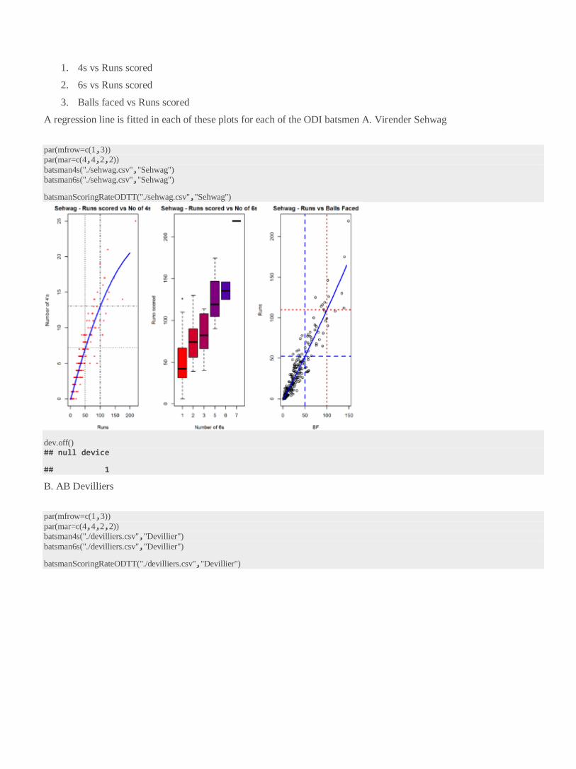
1. 4s vs Runs scored

2. 6s vs Runs scored

3. Balls faced vs Runs scored

A regression line is fitted in each of these plots for each of the ODI batsmen A. Virender Sehwag

par(mfrow=c(1,3)) par(mar=c(4,4,2,2)) batsman4s("./sehwag.csv","Sehwag") batsman6s("./sehwag.csv","Sehwag")

batsmanScoringRateODTT("./sehwag.csv","Sehwag")

dev.off() ## null device

## 1

B. AB Devilliers

par(mfrow=c(1,3)) par(mar=c(4,4,2,2)) batsman4s("./devilliers.csv","Devillier") batsman6s("./devilliers.csv","Devillier")

batsmanScoringRateODTT("./devilliers.csv","Devillier")

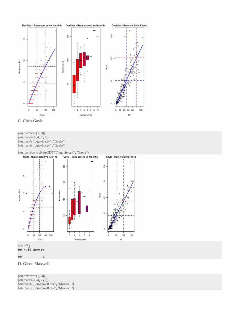
C. Chris Gayle

par(mfrow=c(1,3)) par(mar=c(4,4,2,2)) batsman4s("./gayle.csv","Gayle") batsman6s("./gayle.csv","Gayle")

batsmanScoringRateODTT("./gayle.csv","Gayle")

dev.off() ## null device

## 1

D. Glenn Maxwell

par(mfrow=c(1,3)) par(mar=c(4,4,2,2)) batsman4s("./maxwell.csv","Maxwell") batsman6s("./maxwell.csv","Maxwell")

batsmanScoringRateODTT("./maxwell.csv","Maxwell")

dev.off() ## null device

## 1

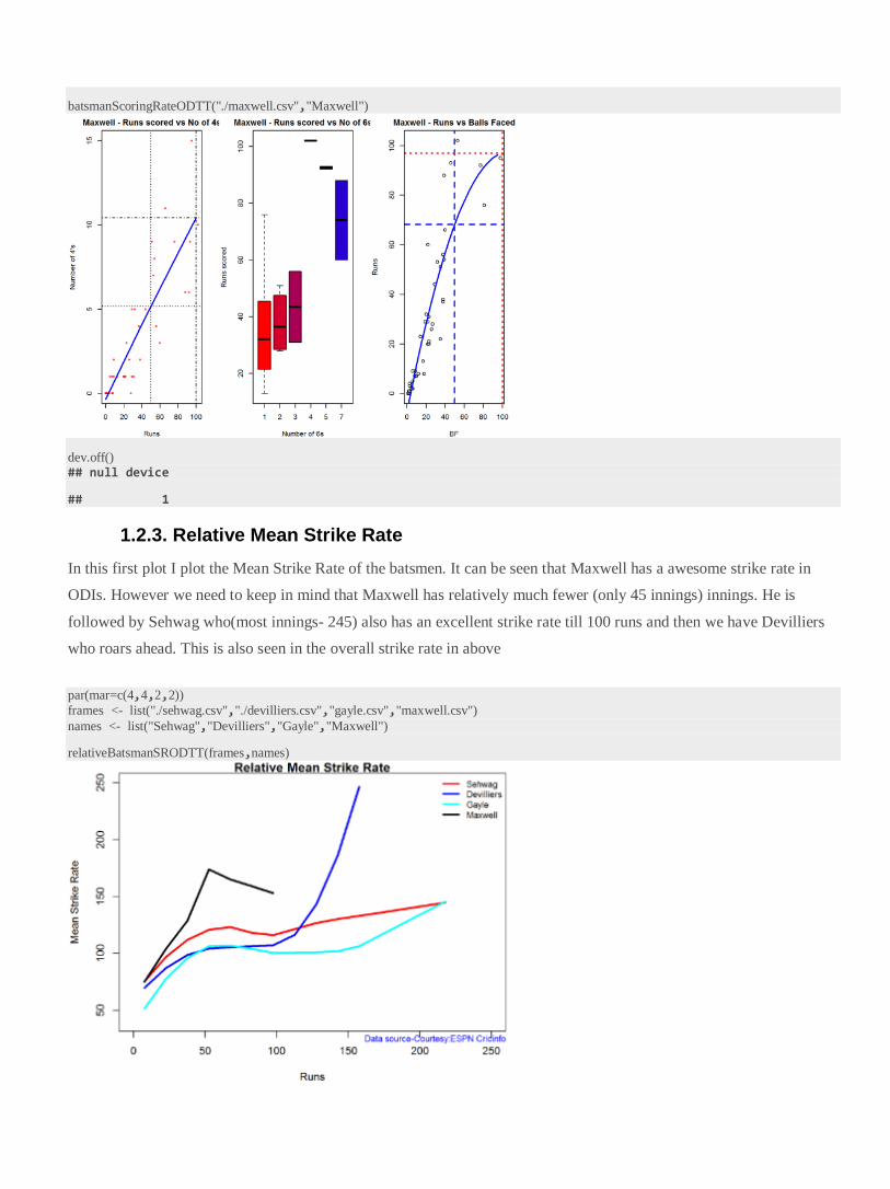
1.2.3. Relative Mean Strike Rate

In this first plot I plot the Mean Strike Rate of the batsmen. It can be seen that Maxwell has a awesome strike rate in

ODIs. However we need to keep in mind that Maxwell has relatively much fewer (only 45 innings) innings. He is

followed by Sehwag who(most innings- 245) also has an excellent strike rate till 100 runs and then we have Devilliers

who roars ahead. This is also seen in the overall strike rate in above

par(mar=c(4,4,2,2)) frames <- list("./sehwag.csv","./devilliers.csv","gayle.csv","maxwell.csv") names <- list("Sehwag","Devilliers","Gayle","Maxwell")

relativeBatsmanSRODTT(frames,names)

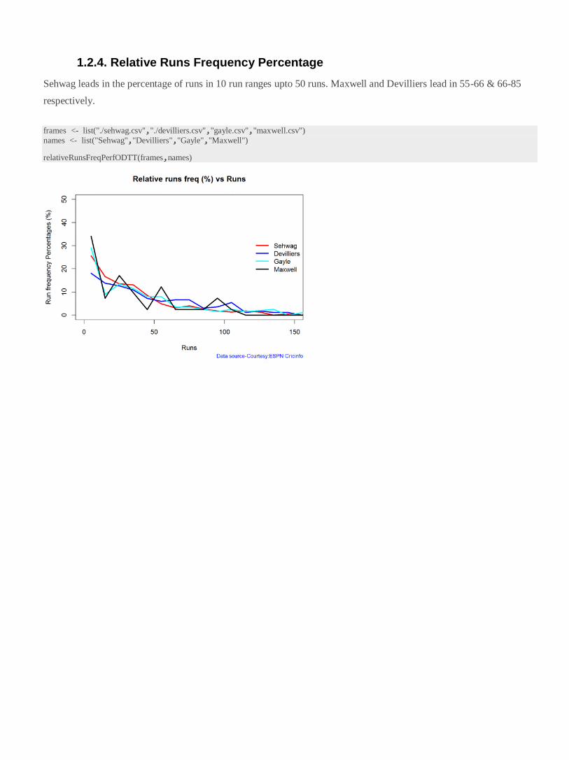
1.2.4. Relative Runs Frequency Percentage

Sehwag leads in the percentage of runs in 10 run ranges upto 50 runs. Maxwell and Devilliers lead in 55-66 & 66-85

respectively.

frames <- list("./sehwag.csv","./devilliers.csv","gayle.csv","maxwell.csv") names <- list("Sehwag","Devilliers","Gayle","Maxwell")

relativeRunsFreqPerfODTT(frames,names)