CRLBs for WSNs localization in NLOS environment

RESEARCH Open Access

CRLBs for WSNs localization in NLOS environmentJiyan Huang1,2*, Peng Wang2 and Qun Wan1

Abstract

Determination of Cramer-Rao lower bound (CRLB) as an optimality criterion for the problem of localization inwireless sensor networks (WSNs) is a very important issue. Currently, CRLBs have been derived for line-of-sight(LOS) situation in WSNs. However, one of major problems for accurate localization in WSNs is non-line-of-sight(NLOS) propagation. This article proposes two CRLBs for WSNs localization in NLOS environment. The proposedCRLBs consider both the cases that positions of reference devices (RDs) are perfectly or imperfectly known. Sincenon-parametric kernel method is used to build probability density function of NLOS errors, the proposed CRLBs aresuitable for various distributions of NLOS errors. Moreover, the proposed CRLBs provide a unified presentation forboth LOS and NLOS environments. Theoretical analysis also proves that the proposed CRLB for NLOS situationbecomes the CRLB for LOS situation when NLOS errors go to 0, which gives a robust check for the proposed CRLB.

Keywords: Wireless sensor networks, Cramer-Rao lower bound, Non-line-of-sight, Node localization

IntroductionWireless sensor networks (WSNs) have been widelyused for monitoring and control in military, environ-mental, health, and commercial systems [1-4]. A WSNusually consists of tens or hundreds of wirelessly con-nected sensors. Sensor positioning becomes an impor-tant issue. Since global positioning system (GPS) iscurrently a costly solution, only a small percentage ofsensors are equipped with GPS receivers called referencedevices (RDs), whereas the other sensors are blindfoldeddevices (BDs).Several methods have been proposed to estimate the

positions of sensors in WSNs. Multi-dimensional scaling(MDS) methods have been successfully applied to theproblem of sensor localization in WSNs [5-7]. Theseclassic MDS approaches based on principal componentanalysis may not scale well with network size as its com-plexity is cubic in the number of sensors. A popularalternative to principal component analysis is the use ofgradient descent or other numerical optimizations[8-10]. The weighted version of MDS in [11] utilized theweighted cost function to improve positioning accuracy.The semi-definite programming algorithm in [12] wasdevised for WSNs localization in the presence of theuncertainties in the positions of RDs. Besides the above

localization algorithms, some studies have been reportedon performance analyses for WSNs localization [12-17].The authors in [13] derived the Cramer-Rao lowerbounds (CRLBs) for the received-signal-strength andtime-of-arrival (TOA) location technologies in WSNs. Amore practical CRLB based on the distance-dependentvariance model for range estimation noise was proposedin [14]. In [16], the clock biases were considered in theCRLB for distributed positioning in sensor network. Theauthors in [17] proposed the CRLB for RD-free localiza-tion and derived the lower and upper bounds on theCRLB. Furthermore, the CRLBs considering the uncer-tainties in the positions of RDs were presented in[12,15].It should be noted that the above studies [5-17] are

based on line-of-sight (LOS) assumption which maylead to severe degradations since non-line-of-sight(NLOS) propagation is a main problem for accuratelocalization in actual WSNs system. In the cellular loca-tion system (CLS) and local positioning system (LPS),some localization methods and performance analyses forNLOS environment have been addressed in the litera-ture [18-26]. The CRLB based on exponential distribu-tion model in [20] cannot be used for otherdistributions of NLOS errors. The CRLB in [21] wasderived for NLOS environment based on a single reflec-tion model, and may not be accurate for a practicalenvironment where most signals arrive at the receiverafter multi-reflections. The CRLB with or without

* Correspondence: [email protected] of Electronic Engineering, University of Electronic Science andTechnology of China, Chengdu, ChinaFull list of author information is available at the end of the article

Huang et al. EURASIP Journal on Wireless Communications and Networking 2011, 2011:16http://jwcn.eurasipjournals.com/content/2011/1/16

© 2011 Huang et al; licensee Springer. This is an Open Access article distributed under the terms of the Creative Commons AttributionLicense (http://creativecommons.org/licenses/by/2.0), which permits unrestricted use, distribution, and reproduction in any medium,provided the original work is properly cited.

mailto:[email protected]

http://creativecommons.org/licenses/by/2.0

NLOS statistics was derived for NLOS situation [22].For the case without NLOS statistics, the authors [22]computed the CRLB in a mixed NLOS/LOS environ-ment and proved that the CRLB for a mixed NLOS/LOS environment depends only on LOS signals. How-ever, the CRLB without NLOS statistics [22] is not sui-table for the situation where measurements from allbase stations are corrupted by NLOS errors. For thecase with NLOS statistics, the authors [22] only pro-vided a definition of CRLB. The detail procedure andformulas for determining the CRLB under various dis-tributions of NLOS errors in a practical environmentwere not considered in [22]. Furthermore, multipatheffects were considered in the CRLB for CLS and LPS[23,24] and the LOS/NLOS unification was discussed in[23,25]. In this article, two CRLBs compatible for var-ious distributions of NLOS errors for WSNs localizationin NLOS environment are proposed. Compared withthe previous performance studies for NLOS situation[20-26], three main contributions of this article arelisted as follows:

1. All the existing CRLBs for NLOS situation weredevised only for CLS and LPS. For a WSNs locationsystem, the problem of sensor localization becomesmore complex since the range measurements amongall sensors are used rather than limited measure-ments between a BD and RDs for a CLS and LPS.The proposed CRLBs considering all of range mea-surements among sensors can be used for not onlyWSNs location system but also CLS and LPS.2. The proposed CRLBs based on non-parametrickernel method can be applicable for different casesincluding various distributions of NLOS errors, sin-gle or multi-reflections model.3. Some characteristics of the CRLBs for WSNs loca-lization are derived in this article. The proposedCRLB provides a unified CRLB presentation for bothLOS and NLOS environments as shown in [21].This means that the previous research results for theCRLB of LOS environment can also be used for theCRLB of NLOS environment. For example, the poi-soning accuracy increases as the more devices areused for sensor localization. Theoretical analysisshows that the CRLB for NLOS environmentbecomes the CRLB for LOS environment in the casethat NLOS errors go to 0, which gives a robustcheck for the proposed CRLB.

This article is organized as follows. Signal model andsome basic notations are presented in next section. Fol-lowed by kernel method is used to estimate the prob-ability density function (PDF) of NLOS errors. Based onthe estimated PDF, CRLBs for NLOS environment are

derived. Next section proves a characteristic of CRLBs.Then, the CRLBs are evaluated by simulations. Finally,conclusions of this article are given.

System modelConsider a TOA-based WSNs location system with n +m devices. Devices 1...n are BDs with the unknowncoordinates, whereas devices n + 1...n + m are RDs withthe known coordinates. Assume that (xi, yi) is the posi-tion of the i th device. The vector of unknown para-meters is:

‚ ‚ ‚= ⎡⎣ ⎤⎦ = [ ]x y n nx x y yT T T T

1 1(1)

As [13], devices may make incomplete observationsdue to the limited link capacity. Let H(i) = {j: device jmakes pair-wise observations with device i}. Note that adevice cannot measure range with itself, so that i ∉ H(i).It is also obvious that if j Î H(i) then i Î H(j).The range measurement rij between the ith and jth

devices can be modeled as:

r d n b d v x x y y vij ij ij ij ij ij i j i j ij= + + = + = −( ) + −( ) +2 2 (2)

where dij is the true distance between the ith and jthdevices, nij represents the Gaussian noise with zero

mean and varianceij

2 , and bij is NLOS error which

may have different statistical distributions in practicalchannel environments. The residual noise is given by

v n bij ij ij= + . It should be noted that Gaussian noise nijand NLOS error bij are independent. This assumptionhas been widely used in the literature [18-20].The CRLB can be used to determine the physical

impossibility of the variance of an unbiased estimatorbeing less than the bound [27]. Let r be a vector ofrange measurements:

r = ( ) +( )⎡⎣ ⎤⎦+ − + − +I r I n m rH H n m n m n m( ) ( ) ( )( )1 12 1 12T

(3)

where IH(k)(l) is an indicator function: 1 if lÎ H (k) or0 otherwise. The CRLB matrix is defined as the inverseof the Fisher information matrix (FIM) J:

E ‚ ‚ ‚ ‚ J−( ) −( )( ) ≥ −T 1 (4)

where ‚ is an estimate of θ.

The FIM is determined by [28]:

Jr ‚‚

r ‚‚

=∂ ( )

∂⋅

∂ ( )∂

⎛

⎝⎜

⎞

⎠⎟

⎡

⎣⎢⎢

⎤

⎦⎥⎥

Ef fln ; ln ;

T

(5)


Page 2 of 14

The log of the joint conditional PDF is:

ln ;( )

f lijj H ij i

i

m n

r ‚( ) =∈<

=

+

∑∑1

(6)

l f r x y x yij ij ij i i j j= ( )( )ln | , , , (7)

Substituting (6) into (5), the FIM can be rewritten as[13]:

JJ JJ J

=⎡

⎣⎢

⎤

⎦⎥

xx xy

xy yy

T (8)

where

J xx kl

kj

kj H k

H k

kl

k

El

xk l

I l El

x

[ ] =

∂∂

⎛

⎝⎜

⎞

⎠⎟

⎡

⎣⎢⎢

⎤

⎦⎥⎥

=

( ) ∂∂

∂

∈∑

2

( )

( )

ll

xk l

El

x

l

y

kl

l

xy kl

kj

k

kj

kj

∂⎡

⎣⎢

⎤

⎦⎥ ≠

⎧

⎨

⎪⎪⎪

⎩

⎪⎪⎪

⎡⎣ ⎤⎦ =

∂∂

∂∂

⎡

⎣⎢

⎤

⎦⎥

∈J

HH k

H k

kl

k

kl

l

yy kl

k l

I l El

x

l

yk l

( )

( )

∑ =

( ) ∂∂

∂∂

⎡

⎣⎢

⎤

⎦⎥ ≠

⎧

⎨

⎪⎪

⎩

⎪⎪

⎡⎣ ⎤⎦ =JEE

l

yk l

I l El

y

l

y

kj

kj H k

H k

kl

k

kl

l

∂∂

⎛

⎝⎜

⎞

⎠⎟

⎡

⎣⎢⎢

⎤

⎦⎥⎥

=

( ) ∂∂

∂∂

⎡

∈∑

2

( )

( )⎣⎣⎢

⎤

⎦⎥ ≠

⎧

⎨

⎪⎪⎪

⎩

⎪⎪⎪

k l

(9)

CRLBs in NLOS environmentModeling range measurementsThe derivation of CRLB is based on the PDF of NLOSerrors. There are two methods for evaluating f(bij). Theparametric method can only be used for specific noisedistributions such as Gaussian, exponential, uniform,and delta distributions. The non-parametric method canbe used for all noise distributions including the PDFwithout explicit expression.The second method is developed to derive the CRLB

for NLOS environment in this article. The basic proce-dure of non-parametric estimation is to create anapproximation of the PDF from a given set of surveymeasurements. Assume that a survey set of NLOS errors{Sbij1...SbijP} with the size P is available for a propagation

channel between the ith and jth devices. The estimatedPDF of bij can be obtained using non-parametric kernelmethod [29]:

f bPh

b Sb

hb

ij

ijt

ijt

P

ij( ) exp= −

−( )⎛

⎝

⎜⎜

⎞

⎠

⎟⎟=

∑1

2 2

2

21

(10)

where exp (·) is a Gaussian kernel function, thesmoothing constant hij is the width of the kernel func-tion which can be determined by using the method in[29]. Simulation results show that Equation 10 can per-fectly estimate the PDF of NLOS errors from the surveyset. Many non-parametric estimators such as histogrammethod, orthogonal series, and other kernel methodscan effectively estimate the PDF and have the similarperformance. Gaussian kernel method was chosen dueto its similarity with the Euclidean distance and alsosince it gives better smoothing and continuous proper-ties even with a small number of samples [30]. Anotherreason for using Gaussian kernel is that the Gaussiankernel function is easy to be integrated and differen-tiated, thereby leads to mathematically tractablesolution.The PDF of Gaussian noise nij is modeled as:

f nn

n ij

ij

ij

ijij( ) exp= −

⎛

⎝⎜⎜

⎞

⎠⎟⎟

1

2 22

2

2 (11)

The PDF of residual noise vij is:

f v f x f v x x

P h

v ij b n ij

ij ij

ij ij ij( ) ( ) ( )

exp

= −

=+( )

−

−∞

+∞

∫ d

1

2 2 2

v Sb

h

ij ijt

ij ijt

P −( )+( )

⎛

⎝⎜⎜

⎞

⎠⎟⎟=

∑2

2 21 2

(12)

Since v r dij ij ij= − , the PDF of rij becomes:

fP h

r d Sb

hij

ij ij

ij ij ijt

ij ij

=+( )

−− −( )

+( )⎛

⎝⎜⎜

⎞

⎠⎟1

2 22 2

2

2 2exp

⎟⎟=∑t

P

1

(13)

CRLB for the case without uncertainty

Substituting (13) into ∂ ∂l xkl k/ and ∂ ∂l ykl k/ , gives:

∂∂

=( )( )

− ∂∂

=( )l

x

g v

f v

x x

d

l

y

g v

f

kl

k

kl kl

v kl

k l

kl

kl

k

kl kl

vkl k

,llv

y y

dkl

k l

kl( )−

(14)


Page 3 of 14

g vP h

v Sb

h

kl kl

kl kl

kl klt

kl kl

( ) =+( )

⋅ −−( )

+( )⎛

⎝⎜

1

2

2

2 2

2

2 2exp

⎜⎜

⎞

⎠⎟⎟

−+=

∑t

Pkl klt

kl kl

v Sb

h12 2

(15)

Similarly,

∂∂

= −( )( )

− ∂∂

= −( )l

x

g v

f v

x x

d

l

y

g v

f

kl

l

kl kl

v kl

k l

kl

kl

l

kl kl

kl

,vv kl

k l

klklv

y y

d( )−

(16)

Substituting (14) and (16) into (9), sub-matrices of Jinclude:

J xx kl

kj

k j

kjj H k

H k kl

k l

kl

Ax x

dk l

I l Ax x

dk

[ ] =

−( )=

− ( ) −( )∈∑

2

2

2

2

( )

( ) ≠≠

⎧

⎨

⎪⎪

⎩

⎪⎪

⎡⎣ ⎤⎦ =

−( ) −( )=

−

∈∑

l

Ax x y y

dk l

I l

xy kl

kj

k j k j

kjj H k

H k

J2

( )

( ) (( ) −( ) −( )≠

⎧

⎨

⎪⎪

⎩

⎪⎪

⎡⎣ ⎤⎦ =

−( )

Ax x y y

dk l

Ay y

d

kl

k l k l

kl

yy kl

kj

k j

kj

2

2

J22

2

2

j H k

H k kl

k l

kl

k l

I l Ay y

dk l

∈∑ =

− ( ) −( )≠

⎧

⎨

⎪⎪

⎩

⎪⎪

( )

( )

(17)

A Eg v

f v

g v

fkl

kl kl

v kl

kl kl

vkl kl

=( )( )

⎛

⎝⎜⎜

⎞

⎠⎟⎟

⎡

⎣

⎢⎢

⎤

⎦

⎥⎥

=( )

2 2

vv

kl

kl( )−∞

+∞

∫ d (18)

Remark 1 Compared with the FIM in [13], the FIM of(17) is similar to the FIM in LOS environment. The

only difference is Akl kl=1 2/ when the FIM is derived

for LOS environment. Thus, Akl can be rewritten as:

A

kl

g v

f vv kl

kl

kl

kl kl

v kl

kl

kl

=

∈

( )( )

∈

⎧

⎨⎪⎪

⎩−∞

+∞

∫

12

2

LOS

d NLOS⎪⎪⎪

(19)

where kl Î LOS means that the propagation pathbetween the devices k and l is a LOS path, otherwiseNLOS path. Equations 17 and 19 give a unified CRLBpresentation for both LOS and NLOS environments.

Remark 2 Either empirical model or survey measure-ments of NLOS errors must be provided since the cor-responding CRLB is derived based on the PDF of NLOSerrors. Many empirical models and survey measure-ments of the PDF of NLOS errors are reported in[31,32].Remark 3 There are virtually no simple parametric

models for the PDF of NLOS errors in all channel envir-onments because its PDF changes as the channel envir-onment changes. It is impossible to derive a CRLBbased on parametric method for practical WSNs loca-tion system. Thus, the proposed CRLBs based on surveymeasurements and non-parametric method are neces-sary since they are applicable for all distributions ofNLOS errors.A particular case where each propagation channel has

the same distribution of NLOS errors is consideredhere. This case will lead to a more compact expressionand deeper understanding of CRLB. In this case,

A Ag v

f vvkl

v

= =( )( )−∞

+∞

∫2

d (20)

From matrix inversion lemma [33], the inverse matrixof J is:

JJ JJ J

J J J J J J J

−

−

− − −

=⎡

⎣⎢

⎤

⎦⎥

=−( )

1

1

1 1 1

xx xy

xy

T

yy

xx xy yy xy

T

xx xy xy

T JJ J J

J J J J J J J J J

xx xy yy

xy

T

xx xy yy xy

T

xx yy xy

T

xx

− −

− − − −

−( )−( ) −

1 1

1 1 1 11 1J xy( )

⎡

⎣

⎢⎢⎢

⎤

⎦

⎥⎥⎥

−

(21)

The CRLB can be written as:

CRLB trace= −( ) + −( ){ }− − − −J J J J J J J Jxx xy yy xy

T

yy xy

T

xx xy

1 1 1 1(22)

where Jxx, Jxy, and Jyy can be obtained from (17).From (17), (20), and (22),

CRLB trace= −( ) + −(− − −1 1 1 1

Axx xy yy xy

T

yy xy

T

xx xyJ J J J J J J J )){ }−1(23)

where

J J

J J

J

xxkl

xx kl A

xykl

xy kl A

yy

kl

kl

⎡⎣ ⎤⎦ = [ ]⎡⎣ ⎤⎦ = ⎡⎣ ⎤⎦⎡⎣ ⎤⎦

=

=

|

|

1

1

kklyy kl Akl

= ⎡⎣ ⎤⎦ =J | 1

(24)

Therefore, the proposed CRLB can be divided intotwo parts. 1/A in (23) depends on Gaussian noise and

NLOS errors while another part consisting of J xx, J xy

,


Page 4 of 14

and J yyis determined by system geometry. For a given

geometry, CRLB is proportional to 1/A. Since theCRLBs for LOS and NLOS situations have the samestructure, the impacts of geometry on the CRLB in LOSenvironment can be applicable for the CRLB in NLOSenvironment. For example, the accuracy increases asmore devices are used for location network.In some special cases, prior information on the loca-

tions of BDs may be available for the system. The fol-lowing CRLB is derived for this case. Assume that thecoordinates of BDs θ = [x1...xn y1...yn]

T are subject to azero-mean Gaussian distribution with covariance matrixQθ. The PDF of (xi,yi), 1 ≤ i ≤ n can be written as:

f xx

f yy

xi i

xi

i

xi

yi i

yi

i

yi

( ) = −⎛

⎝⎜

⎞

⎠⎟

( ) = −

1

2 2

1

2 2

2

2

2

2

exp

exp⎛⎛

⎝⎜⎜

⎞

⎠⎟⎟ ≤ ≤, 1 i n

(25)

where Q‚ = ⎡⎣ ⎤⎦{ }diag x xn y yn12 2

12 2 .

The log of the joint conditional PDF becomes:

l f l l lij

j H ij i

i

m n

xi

i

n

yi

i

n

= = + +∈<

=

+

= =∑∑ ∑ ∑ln

( )1 1 1(26)

where lij can be obtained from (7) and (14), lxi = ln fxi(xi), and lyi = ln fyi (yi).The FIM for the case with prior information on the

locations of BDs can be obtained by substituting (26)

into (5): JJ JJ J

Q‚=⎡

⎣⎢

⎤

⎦⎥ + −xx xy

xy

T

yy

1

where Jxx, Jxy, and Jyy can be obtained from (17).CRLB for the case with uncertaintyThe positions of RDs in a practical system provided byGPS receivers may not be exact due to cost and com-plexity constraints applied on devices. The CRLB con-sidering both NLOS errors and uncertainty of thepositions of RDs is needed.In the presence of disturbances on the positions of

RDs, the position of RDs can be modeled as [12,15]:

x x n

y y n i n n m

i i xi

i i yi

= += + = + +, , ,1

(27)

where the disturbances nxi and nyi are assumed to beindependent zero-mean Gaussian random variables with

variancexi

2 andyi

2 , respectively. The PDF of xi and

yi can be written as:

f xx x

f y

xi i

xi

i i

xi

yi i

yi

( ) = −−( )⎛

⎝⎜⎜

⎞

⎠⎟⎟

( ) = −

1

2 2

1

2

2

2exp

expy yi i

yi

−( )⎛

⎝⎜⎜

⎞

⎠⎟⎟

2

22

(28)

The vector of unknown parameters becomes:

‚ = ⎡⎣ ⎤⎦ = [ ]+( ) + +1 2 1 1n m n m n mx x y yT T (29)

The log of the joint conditional PDF becomes:

l f l l lij

j H ij i

i

m n

xi

i n

n m

yi

i n

n m

= = + +∈<

=

+

= +

+

= +

+

∑∑ ∑ ∑ln( )1 1 1

(30)

Where lij can be obtained from (7) and (14), lxi = ln fxi(xi), and lyi = ln fyi (yi).

Substituting (30) into ∂ ∂l k/ , gives:

∂∂

=

∂∂

≤ ≤

∂∂

+∂∂

< ≤ +

⎧

⎨⎪⎪ ∈ ( )

∈ ( )

∑

∑l

x

l

xk n

l

x

l

xn k n m

k

kj

kj H k

kj

kj H k

xk

k

1

⎩⎩⎪⎪

∂∂

=

∂∂

≤ ≤

∂∂

+∂∂

< ≤ +

∈ ( )

∈ ( )

∑

∑l

y

l

yk n

l

y

l

yn k n m

k

kj

kj H k

kj

kj H k

xk

k

1⎧⎧

⎨⎪⎪

⎩⎪⎪

(31)

To distinguish from the case without uncertainty, G isused as the FIM. Substituting (31) into (5), the FIM canbe rewritten as:

G xx kl

kj

kj H k

kj

k

El

xk l n

El

x[ ] =

∂∂

⎛

⎝⎜

⎞

⎠⎟

⎡

⎣⎢⎢

⎤

⎦⎥⎥

= ≤

∂∂

⎛

⎝⎜

⎞

⎠⎟

∈ ( )∑

2

2⎡⎡

⎣⎢⎢

⎤

⎦⎥⎥

+∂∂

⎛

⎝⎜

⎞

⎠⎟

⎡

⎣⎢⎢

⎤

⎦⎥⎥

< = ≤ +

( )

∈ ( )∑

j H k

xk

k

H k

El

xn k l n m

I l E

2

( )

∂∂∂

∂∂

⎡

⎣⎢

⎤

⎦⎥ ≠

⎧

⎨

⎪⎪⎪⎪⎪

⎩

⎪⎪⎪⎪⎪

l

x

l

xk lkl

k

kl

l

(32)

By symmetry, [Gyy]kl have the same structure as [Gxx]klexcept that the corresponding xk should be replaced byyk. In addition, [Gxy]kl is the same as [Jxy]kl in (9).From (28), the derivatives of lxk and lyk are:

∂∂

=− ∂

∂=

−l

x

x x l

y

y yxk

k

k k

xk

xk

k

k k

yk

2 2, (33)


Page 5 of 14

Substituting (14) and (31) into (32), the FIM becomes:

G J U

G J UG J

xx xx x

yy yy y

xy xy

= +

= +

= (34)

where Jxx, Jxy, and Jyy can be obtained from (17),

U 0 Qy n ydiag= ⎡⎣ ⎤⎦{ }×−

11 , U 0 Qy n ydiag= ⎡⎣ ⎤⎦{ }×

−1

1 ,

Qx x n x n m= ⎡⎣ ⎤⎦{ }+ +diag ( ) ( )12 2 , and

Q y y n y n m= ⎡⎣ ⎤⎦{ }+ +diag ( ) ( )12 2 .

Analysis of CRLBThe authors in [22] proved that the CRLB for the NLOSwill become the CRLB for the LOS when NLOS errors goto 0 in CLS and LPS. However, the problem of sensorlocalization for a WSNs location system becomes morecomplex since the range measurements among all sensorsare used rather than limited measurements between a BDand RDs for a CLS and LPS. Thus, the following Proposi-tion provides theoretical proof for the similar conclusionin WSNs location system. Another purpose of Proposition1 is to give a robust check for the proposed CRLB.Proposition 1 In a WSNs location system, the pro-

posed CRLB for NLOS situation will become the CRLBfor LOS situation in the case that NLOS errors go to 0.Proof Consider the case when all the NLOS errors go

to 0 ( b ijij = ∀0, ) i.e., Sbijt® 0 and hij® 0. The limit of

PDF (12) is

lim ( ) exp,Sb h

v ij

ij

ij

ijijt ij

ijf v

v

→= −

⎛

⎝⎜⎜

⎞

⎠⎟⎟0 2

2

2

1

2 2(35)

The limit of g vij ij( ) is:

lim exp,Sb h

ij ij

ij

ij

ij

ij

ijt ij

g vv v

→( ) = −

⎛

⎝⎜⎜

⎞

⎠⎟⎟0 2

2

2

1

2 2 iij

2 (36)

Then the limit of Aij can be obtained by substituting(35) and (36) into (18):

lim lim, ,Sb h

ijSb h

ij ij

v ij

ijijt ij ijt ij

ij

Ag v

f vv

→ →=

( )( )0 0

2

d−−∞

+∞

∫

= −⎛

⎝⎜⎜

⎞

⎠⎟⎟⎛

⎝⎜⎜

⎞

⎠⎟⎟

1

2 22

2

2 2

2

ij

ij

ij

ij

ij

ij

v vvexp d

−−∞

+∞

−∞

+∞

∫

∫= −⎛

⎝⎜⎜

⎞

⎠⎟⎟

=

1 1

2 2

1

4 2

2

22

ij ij

ij

ij

ij ij

vv vexp d

ij

ij

ij

42

2

1=

(37)

Since g vij ij( ) and f vv ijij( ) are continuous and finite

functions, the integral and limit can switch order in(37). Equation 37 also shows that small values of NLOSerrors will lead to large Aij. It can be seen from (23)that the CRLB is proportional to 1/Aij. Therefore, largeAij will result in small CRLB. It can be seen from (19)and (37) that the proposed CRLB for NLOS environ-ment reduces to the CRLB derived for LOS environmentin [13] when NLOS errors tend to 0. In other words, theCRLB for LOS environment [13] can be interpreted as aspecial case of the proposed CRLB.

Simulation resultsA square region of dimensions 200 m × 200 m is con-sidered for CRLB simulations, where the devices arerandomly deployed. The numbers of RDs and BDs are10 and 50, respectively. The average CRLBs are used toevaluate the performance:

1 1

ntrace J−{ } (38)

1

n n ntrace -1G⎡⎣ ⎤⎦{ }×

(39)

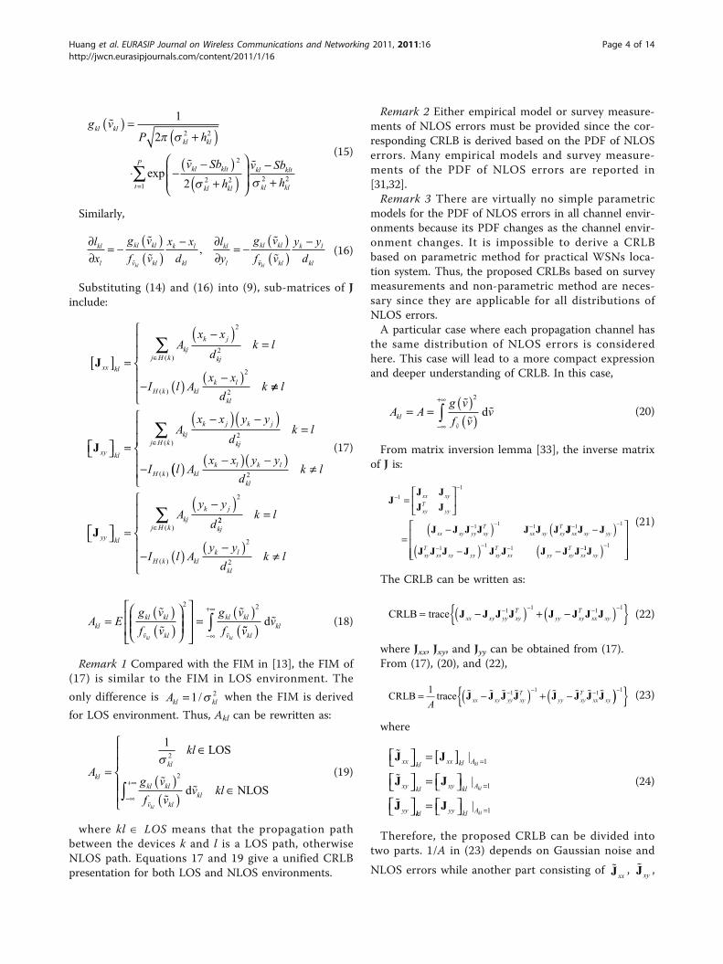
where J and G can be obtained from (17) and (34),respectively. The proposed CRLBs are compared withthe CRLB for LOS situation [13].Case 1: determining the number of samplesThe minimum number of samples for achieving rela-tively accurate results using the derived CRLB is a veryimportant issue. It can be seen from [34] that non-para-metric kernel method can asymptotically converge toany density function with sufficient samples. Thisimplies that the derived CRLBs will converge to theirstable values as the number of samples P increases. Theminimum P can be determined when the derived CRLBsreach their stable values. In this simulation, NLOSerrors are modeled as Rayleigh distribution [32]:

f x

xe x

x

x

( ) = ≥

<

⎧

⎨⎪

⎩⎪

−

22

2

2

0

0 0

(40)

The standard deviation of Gaussian noise is sij = 0.1m and μ is set to 1 which means the mean of NLOSerrors is 1.25 m.Figure 1 shows the derived CRLB versus the number

of samples P. It can be observed that the derived CRLBconverges to a stable value when P ≥ 230. For the casewith insufficient samples, the problem of the determina-tion of the CRLB for WSNs location system in NLOSenvironments will become unsolvable.


Page 6 of 14

Case 2: modeling the PDF of NLOS errors by kernel methodThis experiment is to evaluate the non-parametric ker-nel method for estimating the PDF of NLOS errorsfrom survey data. The number of samples can be deter-mined by substituting the survey data of NLOS errorsinto the derived CRLB and using the method in theabove section.Three different distributions of NLOS errors are con-

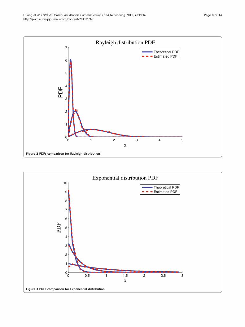
sidered in this simulation. NLOS errors are first mod-eled as Rayleigh distribution, and its PDF can beobtained from (40). The theoretical and estimated PDFsof the Rayleigh distribution with μ = 0.1,0.3,1 using thetheoretical PDF (40) and estimated PDF (10) are plottedin Figure 2. It can be seen that the theoretical and esti-mated PDFs are basically the same with different μ.When NLOS errors are modeled as Exponential distri-

bution [32]:

f xe x

x

x

( ) = ≥

<

⎧⎨⎪

⎩⎪

−10

0 0

(41)

The theoretical and estimated PDFs of the Exponentialdistribution with l = 0.1,0.3,1 using the theoretical PDF(41) and estimated PDF (10) are recorded in Figure 3.Figure 3 also shows kernel method can give a goodapproximation for the PDF of NLOS errors.Compared with parametric estimation method, a

major advantage of the kernel method is that it can beused for the PDF without explicit expression. To verifythis characteristic, NLOS errors are modeled as:

b ab a bij ij ij= + −( )1 (42)

where a is a Bernoulli process with Pr(a = 1) = 0.5.

The bij and bij are the Rayleigh and Exponential ran-

dom variables with μ = 0.3 and l = 0.3, respectively.Since the model of NLOS errors described by (42) has

no explicit expression for PDF, the frequency histogramand estimated PDF are plotted in Figure 4 by matlabfunction “hist” and (10), respectively. Figures 2, 3, and 4show that the proposed equation for PDF estimation(10) is effective.

0 200 400 600 800 10000.01

0.015

0.02

0.025

0.03

0.035

The number of samples

Ave

rage

CR

LB

/m2

NLOS CRLB without uncertainty

Figure 1 NLOS CRLB versus the number of samples.


Page 7 of 14

0 1 2 3 4 50

1

2

3

4

5

6

7

x

PD

F

Rayleigh distribution PDF

Theoretical PDFEstimated PDF

Figure 2 PDFs comparison for Rayleigh distribution.

0 0.5 1 1.5 2 2.5 30

1

2

3

4

5

6

7

8

9

10

x

PDF

Exponential distribution PDF

Theoretical PDFEstimated PDF

Figure 3 PDFs comparison for Exponential distribution.


Page 8 of 14

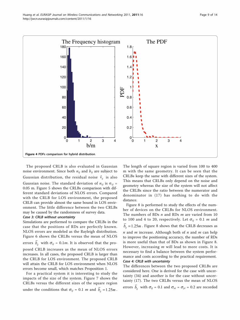
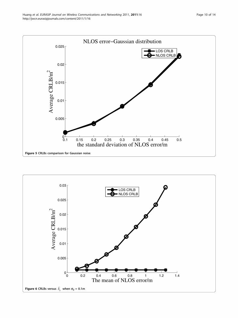
The proposed CRLB is also evaluated in Gaussiannoise environment. Since both nij and bij are subject to

Gaussian distribution, the residual noise vij is also

Gaussian noise. The standard deviation of nij is sij =0.05 m. Figure 5 shows the CRLBs comparison with dif-ferent standard deviations of NLOS errors. Comparedwith the CRLB for LOS environment, the proposedCRLB can provide almost the same bound in LOS envir-onment. The little difference between the two CRLBsmay be caused by the randomness of survey data.Case 3: CRLB without uncertaintySimulations are performed to compare the CRLBs in thecase that the positions of RDs are perfectly known.NLOS errors are modeled as the Rayleigh distribution.Figure 6 shows the CRLBs versus the mean of NLOS

errors bij with sij = 0.1m. It is observed that the pro-

posed CRLB increases as the mean of NLOS errorsincreases. In all cases, the proposed CRLB is larger thanthe CRLB for LOS environment. The proposed CRLBwill attain the CRLB for LOS environment when NLOSerrors become small, which matches Proposition 1.For a practical system it is interesting to study the

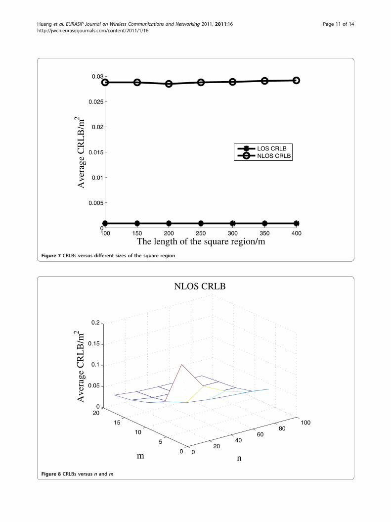
impacts of the size of the system. Figure 7 shows theCRLBs versus the different sizes of the square region

under the conditions that sij = 0.1 m and b mij =1 25. .

The length of square region is varied from 100 to 400m with the same geometry. It can be seen that theCRLBs keep the same with different sizes of the system.This means that CRLBs only depend on the noise andgeometry whereas the size of the system will not affectthe CRLBs since the ratio between the numerator anddenominator in (17) has nothing to do with thedistance.Figure 8 is performed to study the effects of the num-

ber of devices on the CRLBs for NLOS environment.The numbers of BDs n and RDs m are varied from 10to 100 and 4 to 20, respectively. Let sij = 0.1 m and

b mij =1 25. . Figure 8 shows that the CRLB decreases as

n and m increase. Although both of n and m can helpto improve the positioning accuracy, the number of RDsis more useful than that of BDs as shown in Figure 8.However, increasing m will lead to more costs. It isnecessary to find a balance between the system perfor-mance and costs according to the practical requirement.Case 4: CRLB with uncertaintyThe differences between the two proposed CRLBs areconsidered here. One is derived for the case with uncer-tainty (34) and another is for the case without uncer-tainty (17). The two CRLBs versus the mean of NLOS

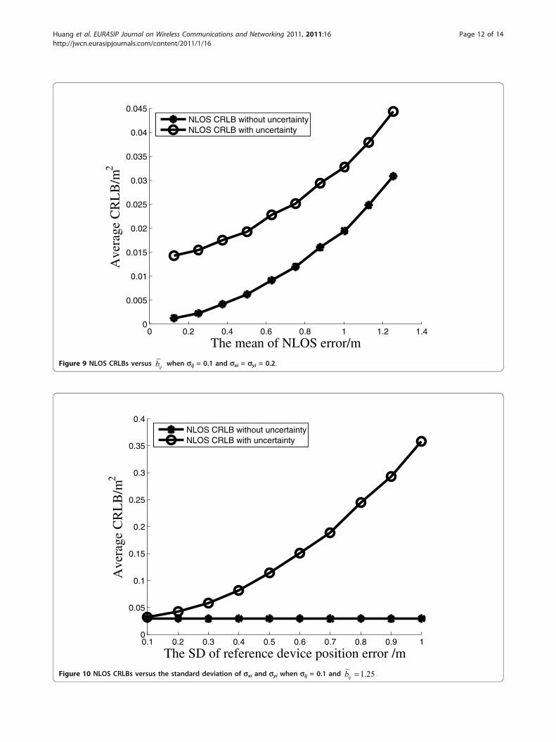
errors bij with sij = 0.1 and sxi = syi = 0.2 are recorded

0 1 2 3 40

20

40

60

80

100

120

140

160

180

b/m

The Frequency histogram

0 1 2 3 40

0.2

0.4

0.6

0.8

1

1.2

1.4

1.6

1.8

x

PDF

The PDF

Figure 4 PDFs comparison for hybrid distribution.


Page 9 of 14

0 0.2 0.4 0.6 0.8 1 1.2 1.40

0.005

0.01

0.015

0.02

0.025

0.03

The mean of NLOS error/m

Ave

rage

CR

LB

/m2

LOS CRLBNLOS CRLB

Figure 6 CRLBs versus bij when sij = 0.1m.

0.1 0.15 0.2 0.25 0.3 0.35 0.4 0.45 0.50

0.005

0.01

0.015

0.02

0.025

the standard deviation of NLOS error/m

Ave

rage

CR

LB

/m2

NLOS error−Gaussian distribution

LOS CRLBNLOS CRLB

Figure 5 CRLBs comparison for Gaussian noise.


Page 10 of 14

100 150 200 250 300 350 4000

0.005

0.01

0.015

0.02

0.025

0.03

The length of the square region/m

Ave

rage

CR

LB

/m2

LOS CRLBNLOS CRLB

Figure 7 CRLBs versus different sizes of the square region.

020

4060

80100

0

5

10

15

200

0.05

0.1

0.15

0.2

n

NLOS CRLB

m

Ave

rage

CR

LB

/m2

Figure 8 CRLBs versus n and m.


Page 11 of 14

0 0.2 0.4 0.6 0.8 1 1.2 1.40

0.005

0.01

0.015

0.02

0.025

0.03

0.035

0.04

0.045

The mean of NLOS error/m

Ave

rage

CR

LB

/m2

NLOS CRLB without uncertaintyNLOS CRLB with uncertainty

Figure 9 NLOS CRLBs versus bij when sij = 0.1 and sxi = syi = 0.2.

0.1 0.2 0.3 0.4 0.5 0.6 0.7 0.8 0.9 10

0.05

0.1

0.15

0.2

0.25

0.3

0.35

0.4

The SD of reference device position error /m

Ave

rage

CR

LB

/m2

NLOS CRLB without uncertaintyNLOS CRLB with uncertainty

Figure 10 NLOS CRLBs versus the standard deviation of sxi and syi when sij = 0.1 and bij =1 25. .


Page 12 of 14

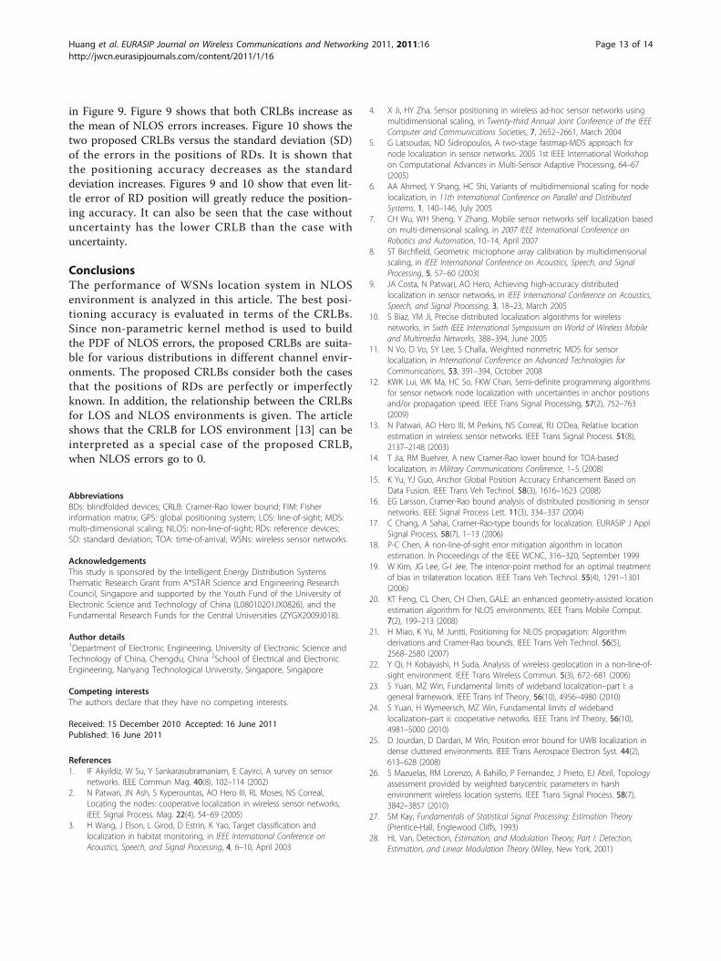
in Figure 9. Figure 9 shows that both CRLBs increase asthe mean of NLOS errors increases. Figure 10 shows thetwo proposed CRLBs versus the standard deviation (SD)of the errors in the positions of RDs. It is shown thatthe positioning accuracy decreases as the standarddeviation increases. Figures 9 and 10 show that even lit-tle error of RD position will greatly reduce the position-ing accuracy. It can also be seen that the case withoutuncertainty has the lower CRLB than the case withuncertainty.

ConclusionsThe performance of WSNs location system in NLOSenvironment is analyzed in this article. The best posi-tioning accuracy is evaluated in terms of the CRLBs.Since non-parametric kernel method is used to buildthe PDF of NLOS errors, the proposed CRLBs are suita-ble for various distributions in different channel envir-onments. The proposed CRLBs consider both the casesthat the positions of RDs are perfectly or imperfectlyknown. In addition, the relationship between the CRLBsfor LOS and NLOS environments is given. The articleshows that the CRLB for LOS environment [13] can beinterpreted as a special case of the proposed CRLB,when NLOS errors go to 0.

AbbreviationsBDs: blindfolded devices; CRLB: Cramer-Rao lower bound; FIM: Fisherinformation matrix; GPS: global positioning system; LOS: line-of-sight; MDS:multi-dimensional scaling; NLOS: non-line-of-sight; RDs: reference devices;SD: standard deviation; TOA: time-of-arrival; WSNs: wireless sensor networks.

AcknowledgementsThis study is sponsored by the Intelligent Energy Distribution SystemsThematic Research Grant from A*STAR Science and Engineering ResearchCouncil, Singapore and supported by the Youth Fund of the University ofElectronic Science and Technology of China (L08010201JX0826), and theFundamental Research Funds for the Central Universities (ZYGX2009J018).

Author details1Department of Electronic Engineering, University of Electronic Science andTechnology of China, Chengdu, China 2School of Electrical and ElectronicEngineering, Nanyang Technological University, Singapore, Singapore

Competing interestsThe authors declare that they have no competing interests.

Received: 15 December 2010 Accepted: 16 June 2011Published: 16 June 2011

References1. IF Akyildiz, W Su, Y Sankarasubramaniam, E Cayirci, A survey on sensor

networks. IEEE Commun Mag. 40(8), 102–114 (2002)2. N Patwari, JN Ash, S Kyperountas, AO Hero III, RL Moses, NS Correal,

Locating the nodes: cooperative localization in wireless sensor networks,IEEE Signal Process. Mag. 22(4), 54–69 (2005)

3. H Wang, J Elson, L Girod, D Estrin, K Yao, Target classification andlocalization in habitat monitoring, in IEEE International Conference onAcoustics, Speech, and Signal Processing, 4, 6–10, April 2003

4. X Ji, HY Zha, Sensor positioning in wireless ad-hoc sensor networks usingmultidimensional scaling, in Twenty-third Annual Joint Conference of the IEEEComputer and Communications Societies, 7, 2652–2661, March 2004

5. G Latsoudas, ND Sidiropoulos, A two-stage fastmap-MDS approach fornode localization in sensor networks. 2005 1st IEEE International Workshopon Computational Advances in Multi-Sensor Adaptive Processing, 64–67(2005)

6. AA Ahmed, Y Shang, HC Shi, Variants of multidimensional scaling for nodelocalization, in 11th International Conference on Parallel and DistributedSystems, 1, 140–146, July 2005

7. CH Wu, WH Sheng, Y Zhang, Mobile sensor networks self localization basedon multi-dimensional scaling, in 2007 IEEE International Conference onRobotics and Automation, 10–14, April 2007

8. ST Birchfield, Geometric microphone array calibration by multidimensionalscaling, in IEEE International Conference on Acoustics, Speech, and SignalProcessing, 5, 57–60 (2003)

9. JA Costa, N Patwari, AO Hero, Achieving high-accuracy distributedlocalization in sensor networks, in IEEE International Conference on Acoustics,Speech, and Signal Processing, 3, 18–23, March 2005

10. S Biaz, YM Ji, Precise distributed localization algorithms for wirelessnetworks, in Sixth IEEE International Symposium on World of Wireless Mobileand Multimedia Networks, 388–394, June 2005

11. N Vo, D Vo, SY Lee, S Challa, Weighted nonmetric MDS for sensorlocalization, in International Conference on Advanced Technologies forCommunications, 53, 391–394, October 2008

12. KWK Lui, WK Ma, HC So, FKW Chan, Semi-definite programming algorithmsfor sensor network node localization with uncertainties in anchor positionsand/or propagation speed. IEEE Trans Signal Processing, 57(2), 752–763(2009)

13. N Patwari, AO Hero III, M Perkins, NS Correal, RJ O’Dea, Relative locationestimation in wireless sensor networks. IEEE Trans Signal Process. 51(8),2137–2148 (2003)

14. T Jia, RM Buehrer, A new Cramer-Rao lower bound for TOA-basedlocalization, in Military Communications Conference, 1–5 (2008)

15. K Yu, YJ Guo, Anchor Global Position Accuracy Enhancement Based onData Fusion. IEEE Trans Veh Technol. 58(3), 1616–1623 (2008)

16. EG Larsson, Cramer-Rao bound analysis of distributed positioning in sensornetworks. IEEE Signal Process Lett. 11(3), 334–337 (2004)

17. C Chang, A Sahai, Cramer-Rao-type bounds for localization. EURASIP J ApplSignal Process. 58(7), 1–13 (2006)

18. P-C Chen, A non-line-of-sight error mitigation algorithm in locationestimation. In Proceedings of the IEEE WCNC, 316–320, September 1999

19. W Kim, JG Lee, G-I Jee, The interior-point method for an optimal treatmentof bias in trilateration location. IEEE Trans Veh Technol. 55(4), 1291–1301(2006)

20. KT Feng, CL Chen, CH Chen, GALE: an enhanced geometry-assisted locationestimation algorithm for NLOS environments. IEEE Trans Mobile Comput.7(2), 199–213 (2008)

21. H Miao, K Yu, M Juntti, Positioning for NLOS propagation: Algorithmderivations and Cramer-Rao bounds. IEEE Trans Veh Technol. 56(5),2568–2580 (2007)

22. Y Qi, H Kobayashi, H Suda, Analysis of wireless geolocation in a non-line-of-sight environment. IEEE Trans Wireless Commun. 5(3), 672–681 (2006)

23. S Yuan, MZ Win, Fundamental limits of wideband localization–part I: ageneral framework. IEEE Trans Inf Theory, 56(10), 4956–4980 (2010)

24. S Yuan, H Wymeersch, MZ Win, Fundamental limits of widebandlocalization–part ii: cooperative networks. IEEE Trans Inf Theory, 56(10),4981–5000 (2010)

25. D Jourdan, D Dardari, M Win, Position error bound for UWB localization indense cluttered environments. IEEE Trans Aerospace Electron Syst. 44(2),613–628 (2008)

26. S Mazuelas, RM Lorenzo, A Bahillo, P Fernandez, J Prieto, EJ Abril, Topologyassessment provided by weighted barycentric parameters in harshenvironment wireless location systems. IEEE Trans Signal Process. 58(7),3842–3857 (2010)

27. SM Kay, Fundamentals of Statistical Signal Processing: Estimation Theory(Prentice-Hall, Englewood Cliffs, 1993)

28. HL Van, Detection, Estimation, and Modulation Theory, Part I: Detection,Estimation, and Linear Modulation Theory (Wiley, New York, 2001)


Page 13 of 14

29. M Mcguire, KN Platuniotis, AN Venetsanopoulos, Location of mobileterminals using time measurements and survey points. IEEE Trans VehTechnol. 52(4), 999–1011 (2003)

30. A Elgammal, R Duraiswami, D Harwood, LS Davis, Background andforeground modeling using nonparametric kernel density estimation forvisual surveillance. Proc IEEE. 90(7), 1151–1163 (2002)

31. G Destino, D Macagnano, GTF de Abreu, Hypothesis testing and iterativeWLS minimization for WSN localization under LOS/NLOS conditions, in TheForty-First Asilomar Conference on Signals, Systems and Computers,2150–2155, November 2007

32. J Prieto, A Bahillo, S Mazuelas, RM Lorenzo, J Blas, P Fernandez, NLOSmitigation based on range estimation error characterization in an RTT-based IEEE 802.11, indoor location system. IEEE International Symposium onIntelligent Signal Processing, 61–66 (2009)

33. RA Horn, CR Johnson, Matrix Analysis, (Cambridge University Press,Cambridge, 1999)

34. A Elgammal, R Duraiswami, D Harwood, LS Davis, Background andforeground modeling using nonparametric kernel density estimation forvisual surveillance. Proc IEEE. 90(7), 1151–1163 (2002)

doi:10.1186/1687-1499-2011-16Cite this article as: Huang et al.: CRLBs for WSNs localization in NLOSenvironment. EURASIP Journal on Wireless Communications and Networking2011 2011:16.

Submit your manuscript to a journal and benefi t from:

7 Convenient online submission

7 Rigorous peer review

7 Immediate publication on acceptance

7 Open access: articles freely available online

7 High visibility within the fi eld

7 Retaining the copyright to your article

Submit your next manuscript at 7 springeropen.com


Page 14 of 14

http://www.springeropen.com/

http://www.springeropen.com/

Documents

CRLBs for WSNs localization in NLOS environment