Lee CSCE 314 TAMU

1

CSCE 314Programming Languages

Final Review Part I

Dr. Hyunyoung Lee

Lee CSCE 314 TAMU

2

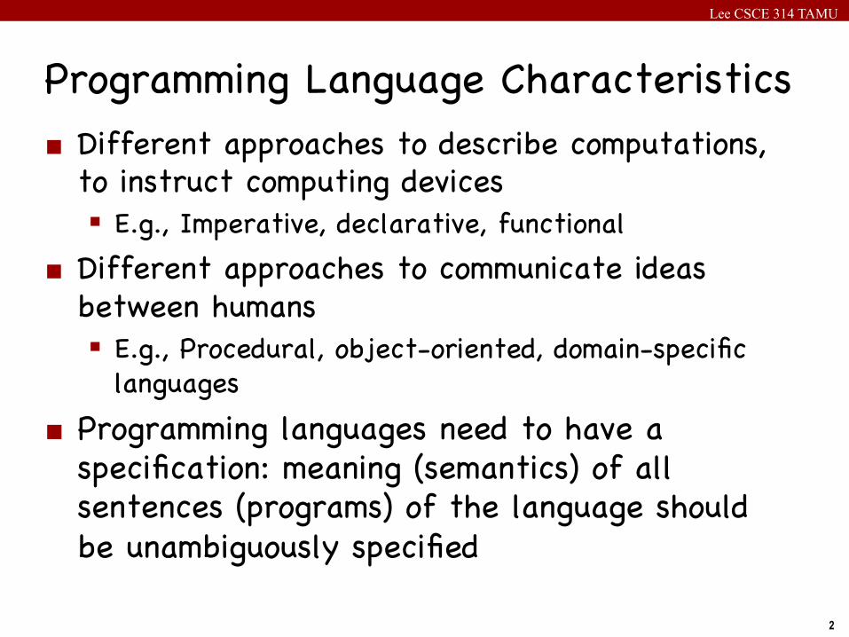
Programming Language Characteristics¢  Different approaches to describe computations,

to instruct computing devices§  E.g., Imperative, declarative, functional

¢  Different approaches to communicate ideas between humans§  E.g., Procedural, object-oriented, domain-specific

languages¢  Programming languages need to have a

specification: meaning (semantics) of all sentences (programs) of the language should be unambiguously specified

Lee CSCE 314 TAMU

3

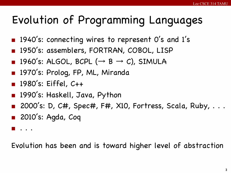
Evolution of Programming Languages¢  1940’s: connecting wires to represent 0’s and 1’s¢  1950’s: assemblers, FORTRAN, COBOL, LISP¢  1960’s: ALGOL, BCPL (→ B → C), SIMULA¢  1970’s: Prolog, FP, ML, Miranda¢  1980’s: Eiffel, C++¢  1990’s: Haskell, Java, Python¢  2000’s: D, C#, Spec#, F#, X10, Fortress, Scala, Ruby, . . .¢  2010’s: Agda, Coq¢  . . .

Evolution has been and is toward higher level of abstraction

Lee CSCE 314 TAMU

4

Implementing a Programming Language – How to Undo the Abstraction

Sourceprogram

Lexer Parser Typechecker

Interpreter

Op8mizer

Codegenerator

Machinecode

Bytecode

Machine

VirtualmachineI/O

JIT

I/O

I/O

Lee CSCE 314 TAMU

5

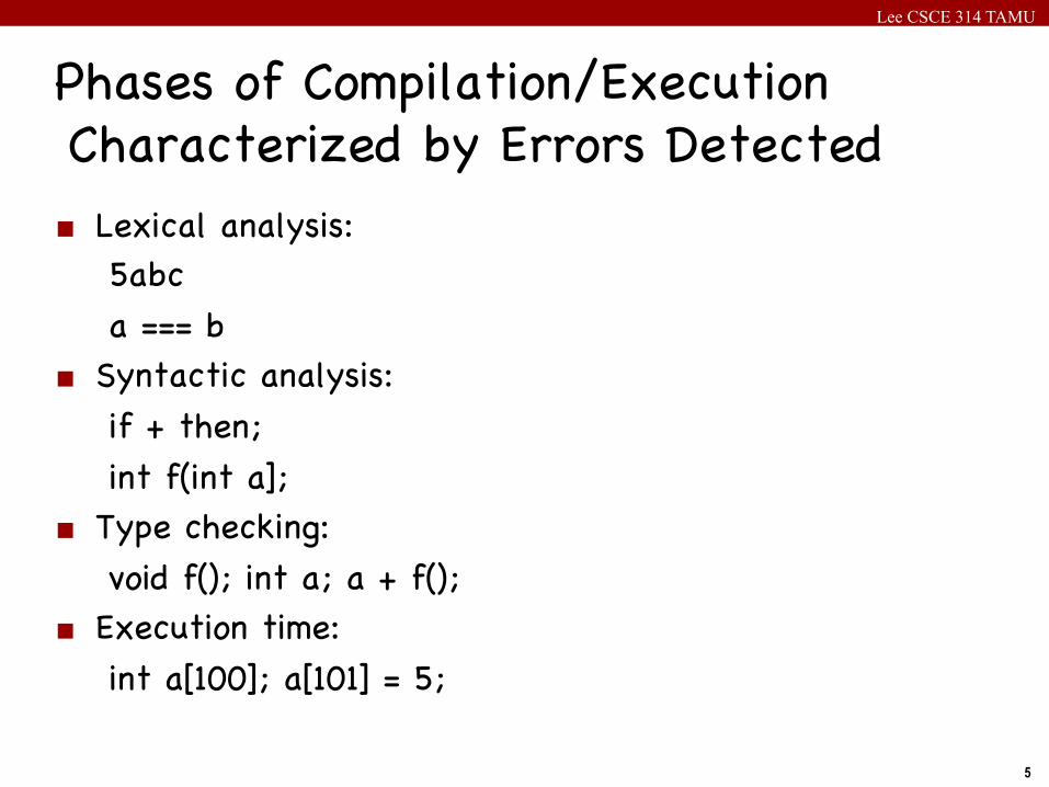
Phases of Compilation/Execution Characterized by Errors Detected

¢  Lexical analysis:5abca === b

¢  Syntactic analysis:if + then;int f(int a];

¢  Type checking:void f(); int a; a + f();

¢  Execution time:int a[100]; a[101] = 5;

Lee CSCE 314 TAMU

6

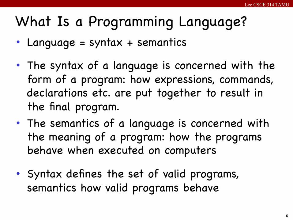
•  Language = syntax + semantics

•  The syntax of a language is concerned with the form of a program: how expressions, commands, declarations etc. are put together to result in the final program.

•  The semantics of a language is concerned with the meaning of a program: how the programs behave when executed on computers

•  Syntax defines the set of valid programs, semantics how valid programs behave

What Is a Programming Language?

Lee CSCE 314 TAMU

7

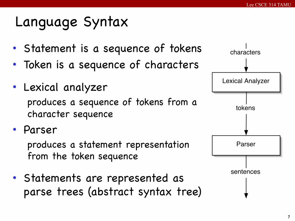
•  Statement is a sequence of tokens•  Token is a sequence of characters

•  Lexical analyzerproduces a sequence of tokens from a character sequence

•  Parserproduces a statement representation from the token sequence

•  Statements are represented as parse trees (abstract syntax tree)

Language Syntax Syntax

Language Syntax

Statement is a sequence of tokensToken is a sequence of charactersLexical analyzer:

produces a token sequence from acharacter sequence

Parserproduces a statement representationfrom a token sequence

Statements are represented as parsetrees (abstract syntax trees)

Lexical Analyzer

Parser

characters

tokens

sentences

8 / 33

Lee CSCE 314 TAMU

8

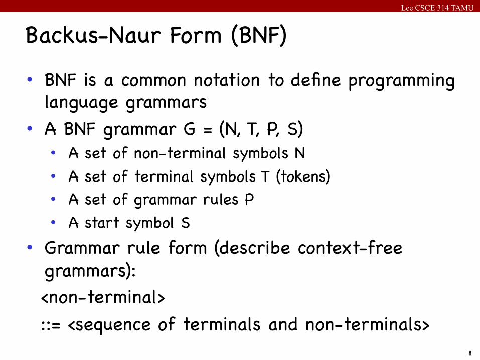
•  BNF is a common notation to define programming language grammars

•  A BNF grammar G = (N, T, P, S) •  A set of non-terminal symbols N•  A set of terminal symbols T (tokens)•  A set of grammar rules P•  A start symbol S

•  Grammar rule form (describe context-free grammars):

<non-terminal> ::= <sequence of terminals and non-terminals>

Backus-Naur Form (BNF)

Lee CSCE 314 TAMU

9

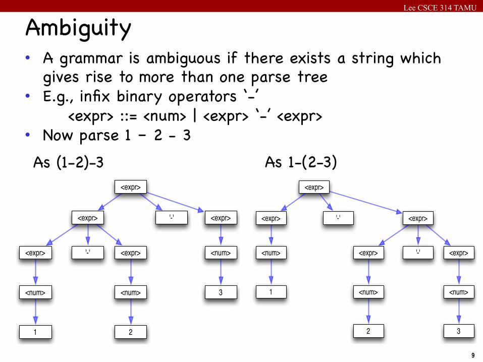
•  A grammar is ambiguous if there exists a string which gives rise to more than one parse tree

•  E.g., infix binary operators ‘-’ <expr> ::= <num> | <expr> ‘-’ <expr>•  Now parse 1 – 2 - 3

Ambiguity

As (1-2)-3 As 1-(2-3)

Parsing

Parse 1

As (1 - 2) - 3:

<expr>

'-'<expr> <expr>

'-'

<num>

<expr>

2

<expr> <num>

3

1

<num>

20 / 33

Parsing

Parse 2

As 1 - (2 - 3):

<expr>

'-' <expr><expr>

'-'

<num>

<expr>

3

<expr><num>

1

2

<num>

21 / 33

Lee CSCE 314 TAMU

10

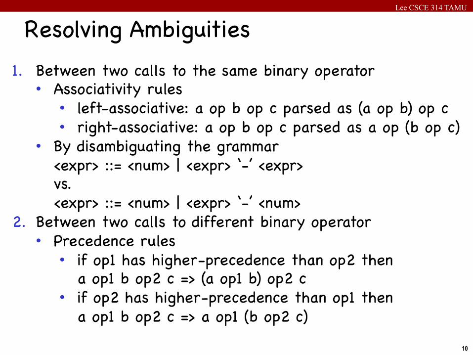
1.  Between two calls to the same binary operator•  Associativity rules•  left-associative: a op b op c parsed as (a op b) op c•  right-associative: a op b op c parsed as a op (b op c)

•  By disambiguating the grammar <expr> ::= <num> | <expr> ‘-’ <expr> vs. <expr> ::= <num> | <expr> ‘-’ <num>

2.  Between two calls to different binary operator•  Precedence rules•  if op1 has higher-precedence than op2 then a op1 b op2 c => (a op1 b) op2 c•  if op2 has higher-precedence than op1 then a op1 b op2 c => a op1 (b op2 c)

Resolving Ambiguities

Lee CSCE 314 TAMU

11

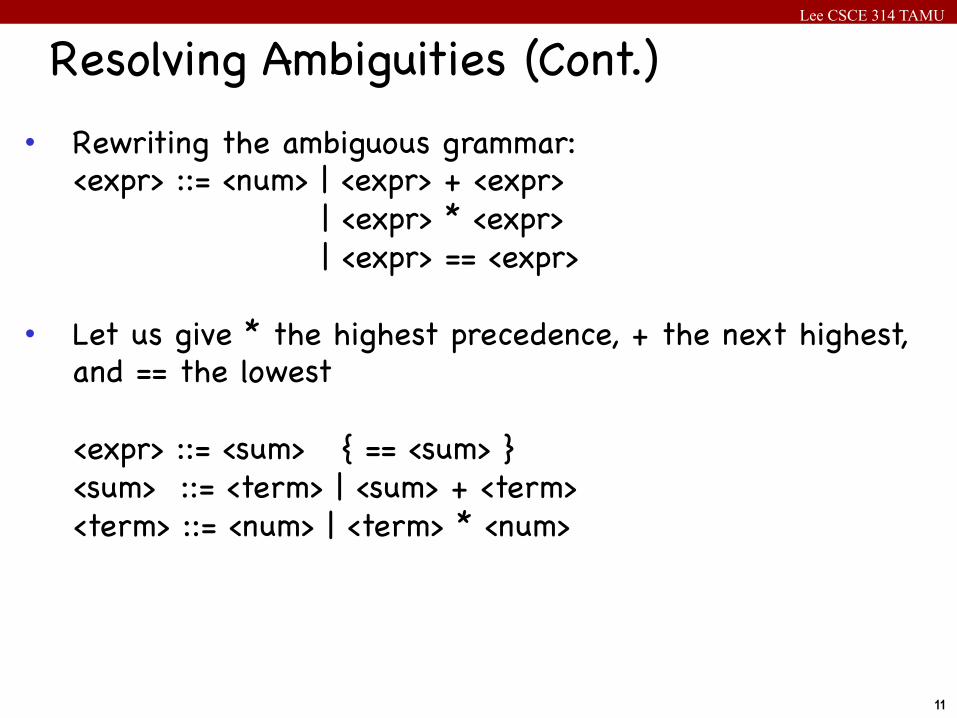
•  Rewriting the ambiguous grammar: <expr> ::= <num> | <expr> + <expr> | <expr> * <expr> | <expr> == <expr>

•  Let us give * the highest precedence, + the next highest,

and == the lowest

<expr> ::= <sum> { == <sum> } <sum> ::= <term> | <sum> + <term> <term> ::= <num> | <term> * <num>

Resolving Ambiguities (Cont.)

Lee CSCE 314 TAMU

12

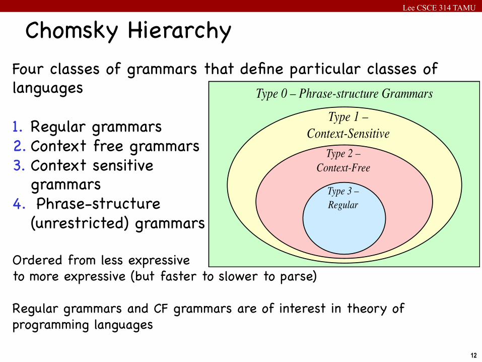
Four classes of grammars that define particular classes of languages 1.  Regular grammars2. Context free grammars3. Context sensitive grammars4.  Phrase-structure (unrestricted) grammarsOrdered from less expressive to more expressive (but faster to slower to parse)Regular grammars and CF grammars are of interest in theory ofprogramming languages

Chomsky Hierarchy

Type 0 – Phrase-structure Grammars

Type 1 – Context-Sensitive

Type 2 –Context-Free

Type 3 –Regular

Lee CSCE 314 TAMU

13

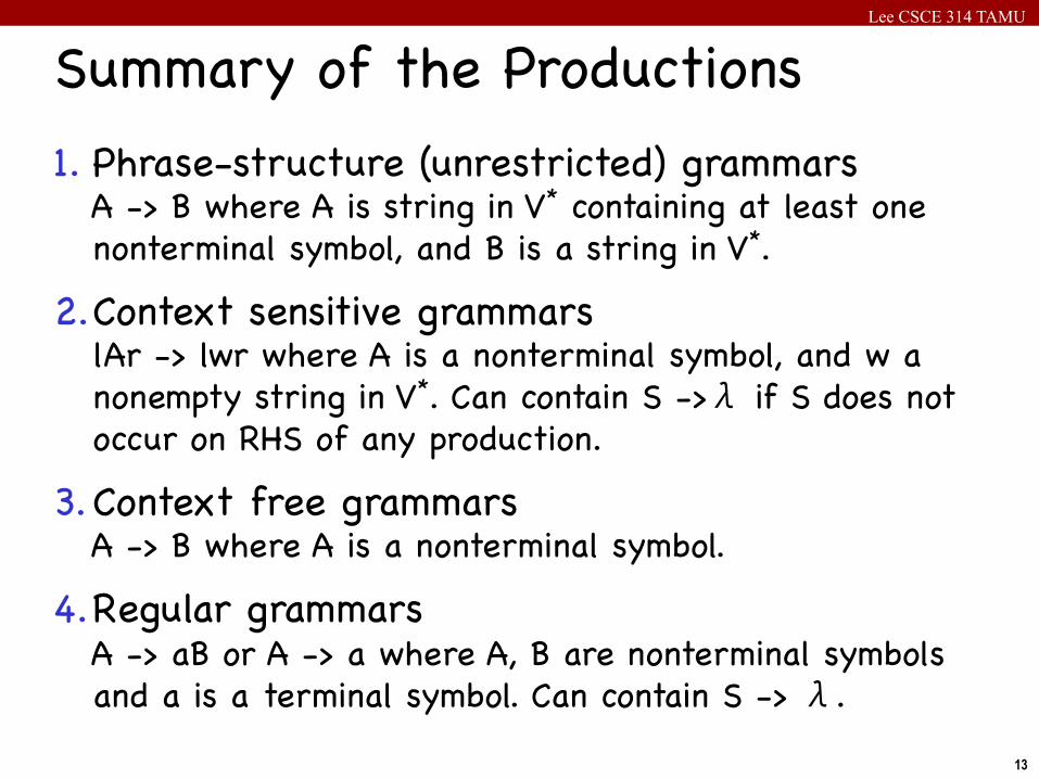
1. Phrase-structure (unrestricted) grammars A -> B where A is string in V* containing at least one nonterminal symbol, and B is a string in V*.

2. Context sensitive grammars lAr -> lwr where A is a nonterminal symbol, and w a nonempty string in V*. Can contain S ->λ if S does not occur on RHS of any production.

3. Context free grammars A -> B where A is a nonterminal symbol.

4. Regular grammars A -> aB or A -> a where A, B are nonterminal symbols and a is a terminal symbol. Can contain S -> λ.

Summary of the Productions

Lee CSCE 314 TAMU

14

HaskellLazyPure

Functional Language

Lee CSCE 314 TAMU

15

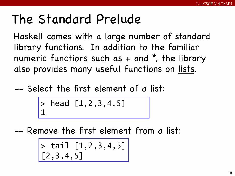
The Standard PreludeHaskell comes with a large number of standard library functions. In addition to the familiar numeric functions such as + and *, the library also provides many useful functions on lists.

-- Select the first element of a list:> head [1,2,3,4,5] 1

-- Remove the first element from a list:> tail [1,2,3,4,5] [2,3,4,5]

Lee CSCE 314 TAMU

16

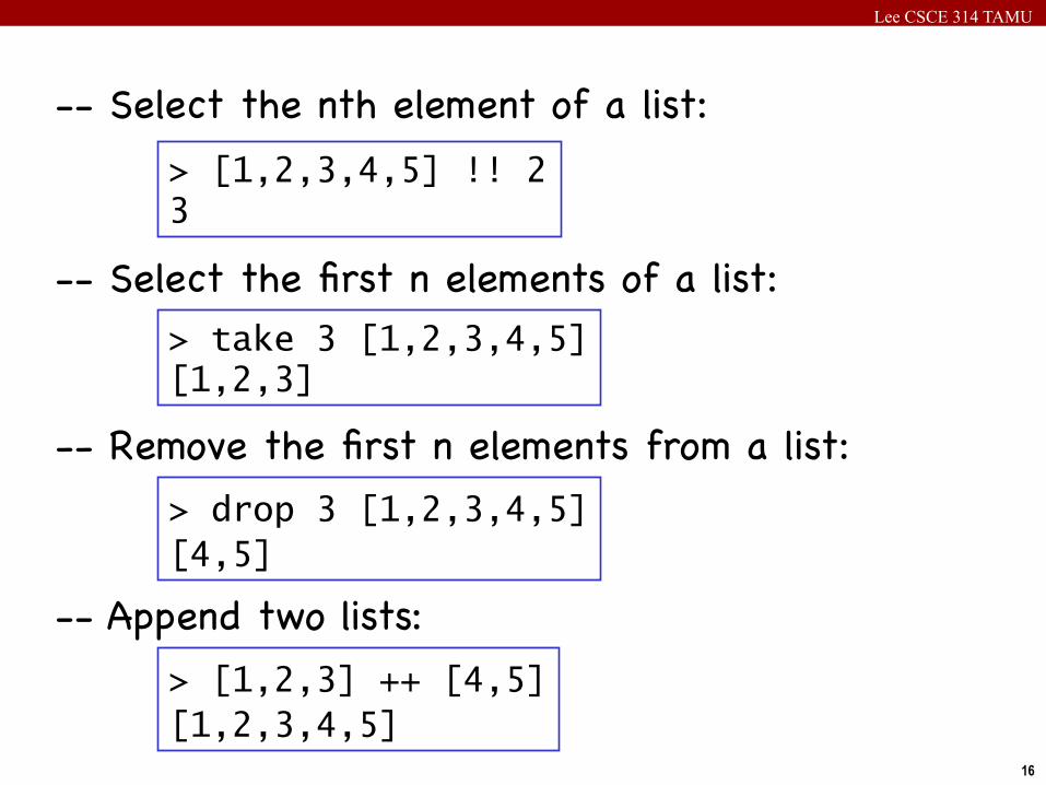
-- Select the nth element of a list:> [1,2,3,4,5] !! 2 3

-- Select the first n elements of a list:> take 3 [1,2,3,4,5] [1,2,3]

-- Remove the first n elements from a list:> drop 3 [1,2,3,4,5] [4,5]

-- Append two lists:> [1,2,3] ++ [4,5] [1,2,3,4,5]

Lee CSCE 314 TAMU

17

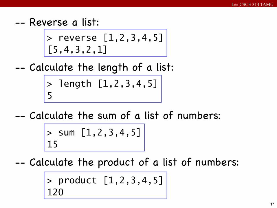
-- Calculate the length of a list:> length [1,2,3,4,5] 5

-- Calculate the sum of a list of numbers:> sum [1,2,3,4,5] 15

-- Calculate the product of a list of numbers:> product [1,2,3,4,5] 120

-- Reverse a list:> reverse [1,2,3,4,5] [5,4,3,2,1]

Lee CSCE 314 TAMU

18

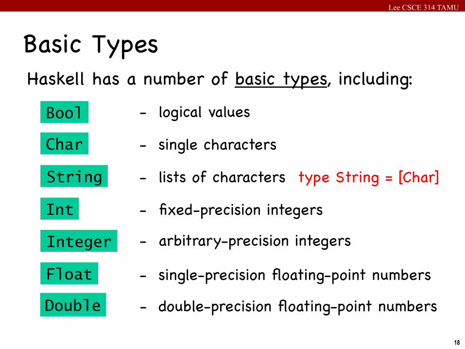
Basic TypesHaskell has a number of basic types, including:

Bool - logical values

Char - single characters

Integer - arbitrary-precision integers

Float - single-precision floating-point numbers

String - lists of characters type String = [Char]

Int - fixed-precision integers

Double - double-precision floating-point numbers

Lee CSCE 314 TAMU

19

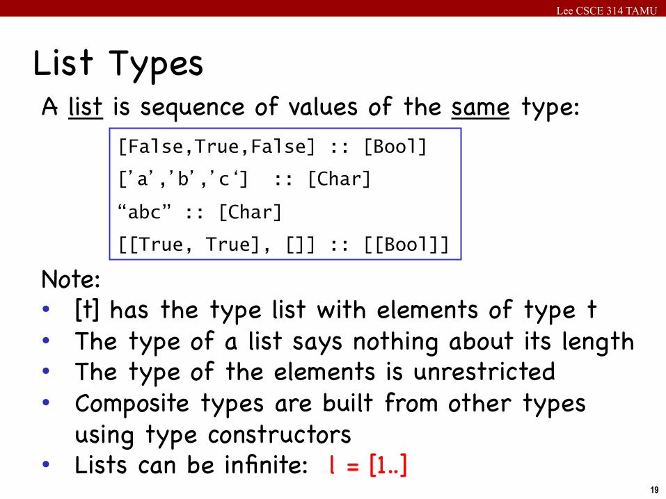
List Types

[False,True,False] :: [Bool]

[’a’,’b’,’c‘] :: [Char]

“abc” :: [Char]

[[True, True], []] :: [[Bool]]

A list is sequence of values of the same type:

Note:•  [t] has the type list with elements of type t•  The type of a list says nothing about its length•  The type of the elements is unrestricted•  Composite types are built from other types

using type constructors•  Lists can be infinite: l = [1..]

Lee CSCE 314 TAMU

20

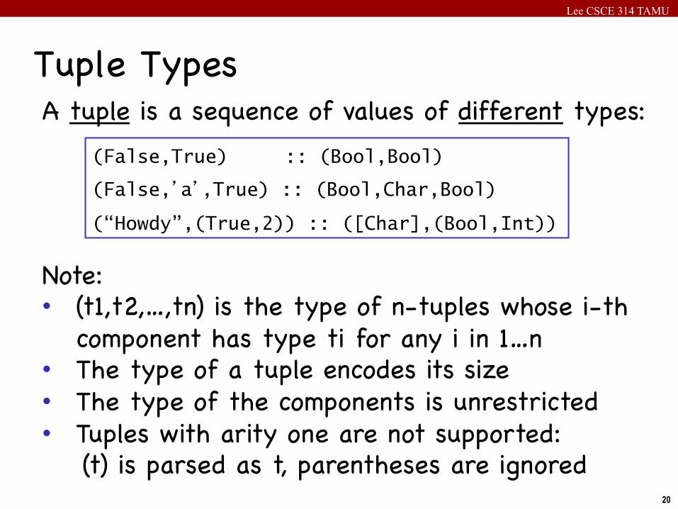
Tuple TypesA tuple is a sequence of values of different types:

Note:•  (t1,t2,…,tn) is the type of n-tuples whose i-th

component has type ti for any i in 1…n•  The type of a tuple encodes its size•  The type of the components is unrestricted•  Tuples with arity one are not supported: (t) is parsed as t, parentheses are ignored

(False,True) :: (Bool,Bool)

(False,’a’,True) :: (Bool,Char,Bool)

(“Howdy”,(True,2)) :: ([Char],(Bool,Int))

Lee CSCE 314 TAMU

21

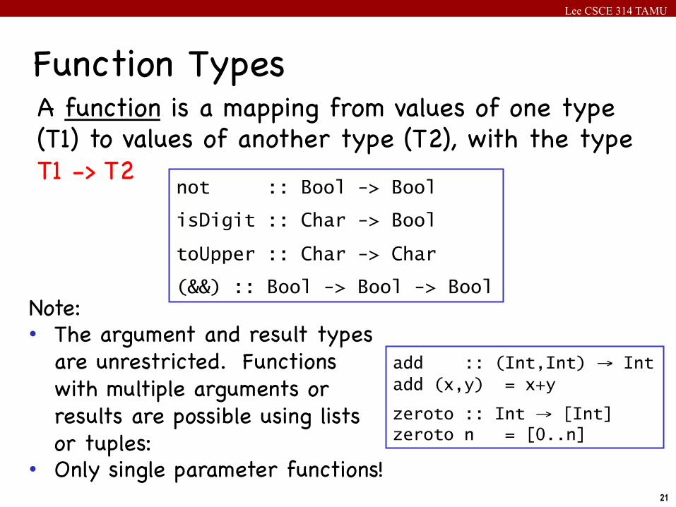
Function Types

not :: Bool -> Bool

isDigit :: Char -> Bool

toUpper :: Char -> Char

(&&) :: Bool -> Bool -> Bool Note: •  The argument and result types

are unrestricted. Functions with multiple arguments or results are possible using lists or tuples:

•  Only single parameter functions!

A function is a mapping from values of one type (T1) to values of another type (T2), with the type T1 -> T2

add :: (Int,Int) → Int add (x,y) = x+y

zeroto :: Int → [Int] zeroto n = [0..n]

Lee CSCE 314 TAMU

22

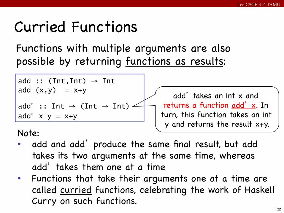
Curried FunctionsFunctions with multiple arguments are also possible by returning functions as results:add :: (Int,Int) → Int add (x,y) = x+y

add’ :: Int → (Int → Int) add’ x y = x+y

add’ takes an int x and returns a function add’ x. In turn, this function takes an int y and returns the result x+y.

Note:•  add and add’ produce the same final result, but add

takes its two arguments at the same time, whereas add’ takes them one at a time

•  Functions that take their arguments one at a time are called curried functions, celebrating the work of Haskell Curry on such functions.

Lee CSCE 314 TAMU

23

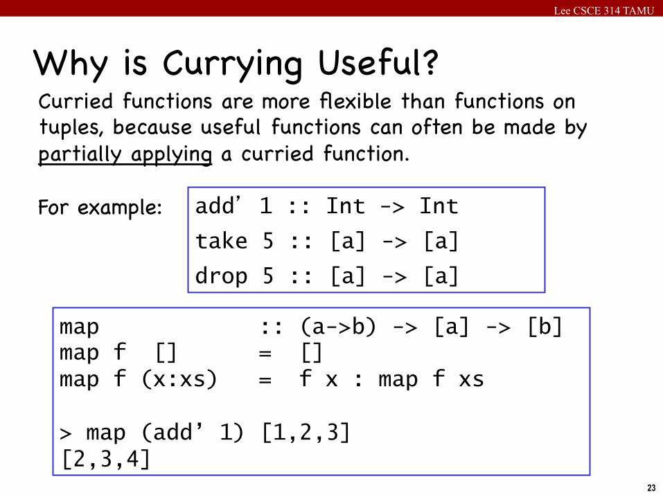
Why is Currying Useful?Curried functions are more flexible than functions on tuples, because useful functions can often be made by partially applying a curried function.For example: add’ 1 :: Int -> Int

take 5 :: [a] -> [a]

drop 5 :: [a] -> [a]

map :: (a->b) -> [a] -> [b] map f  [] =  [] map f (x:xs) =  f x : map f xs > map (add’ 1) [1,2,3] [2,3,4]

Lee CSCE 314 TAMU

24

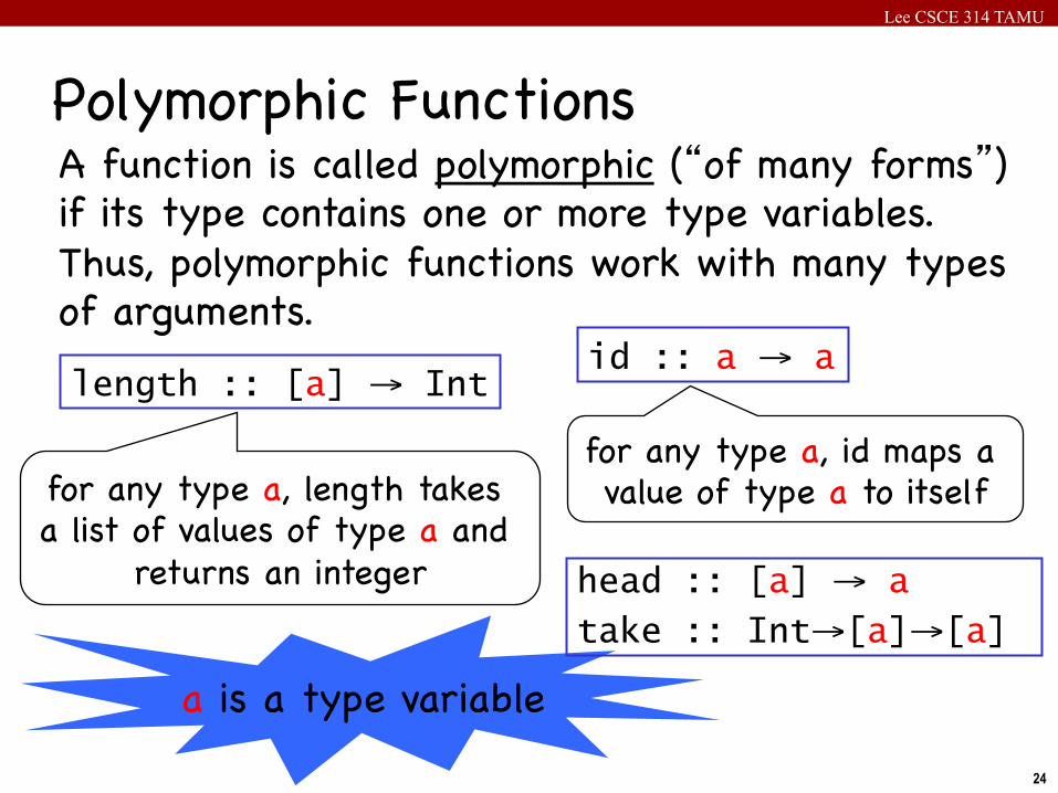
Polymorphic FunctionsA function is called polymorphic (“of many forms”) if its type contains one or more type variables. Thus, polymorphic functions work with many types of arguments.

id :: a → a

for any type a, length takes a list of values of type a and

returns an integer

length :: [a] → Int

for any type a, id maps a value of type a to itself

a is a type variable

head :: [a] → a

take :: Int→[a]→[a]

Lee CSCE 314 TAMU

25

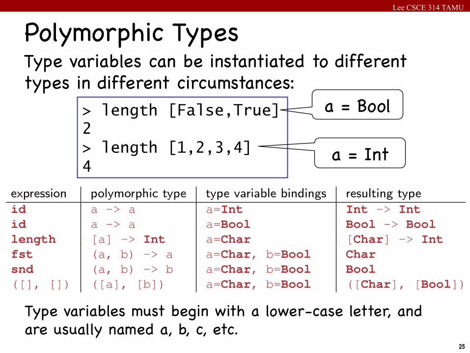
Type variables can be instantiated to different types in different circumstances:

Type variables must begin with a lower-case letter, and are usually named a, b, c, etc.

> length [False,True] 2

> length [1,2,3,4] 4

a = Bool

a = Int

Polymorphic types and type variables

A polymorphic type is a type that contains one or more type variablesThink of it as a schema or template from which to instantiate othertypes by binding values to the type variables

expression polymorphic type type variable bindings resulting typeid a -> a a=Int Int -> Intid a -> a a=Bool Bool -> Boollength [a] -> Int a=Char [Char] -> Intfst (a, b) -> a a=Char, b=Bool Charsnd (a, b) -> b a=Char, b=Bool Bool([], []) ([a], [b]) a=Char, b=Bool ([Char], [Bool])

Type variables must start with lowercase lettersTypical conventions: a, b, c, . . . , t, u, . . . , a1, a2, . . . , a’, a’’,. . .

Jaakko Järvi (TAMU) Programming Languages CSCE-314 September 5, 2012 42 / 49

Polymorphic Types

Lee CSCE 314 TAMU

26

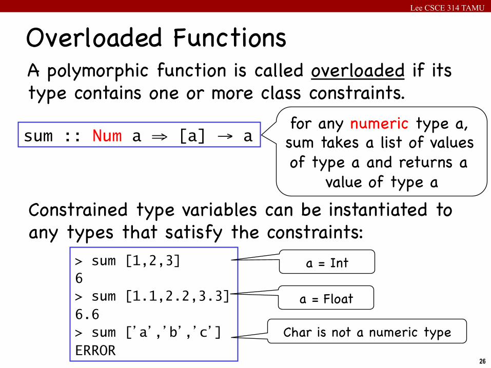
Overloaded FunctionsA polymorphic function is called overloaded if its type contains one or more class constraints.

sum :: Num a ⇒ [a] → a for any numeric type a, sum takes a list of values of type a and returns a

value of type aConstrained type variables can be instantiated to any types that satisfy the constraints:

> sum [1,2,3] 6 > sum [1.1,2.2,3.3] 6.6 > sum [’a’,’b’,’c’] ERROR

Char is not a numeric type

a = Int

a = Float

Lee CSCE 314 TAMU

27

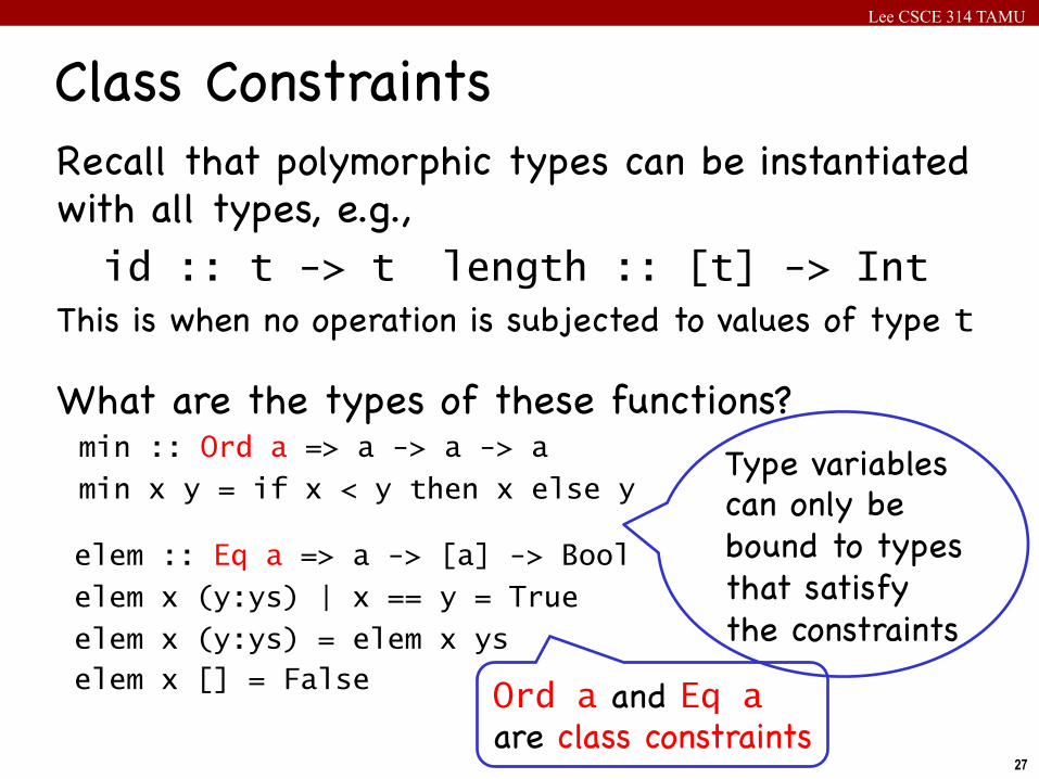
Recall that polymorphic types can be instantiated with all types, e.g., id :: t -> t length :: [t] -> Int This is when no operation is subjected to values of type t

What are the types of these functions? min :: Ord a => a -> a -> a min x y = if x < y then x else y

elem :: Eq a => a -> [a] -> Bool

elem x (y:ys) | x == y = True

elem x (y:ys) = elem x ys elem x [] = False

Class Constraints

Ord a and Eq a are class constraints

Type variables can only be bound to types that satisfy the constraints

Lee CSCE 314 TAMU

28

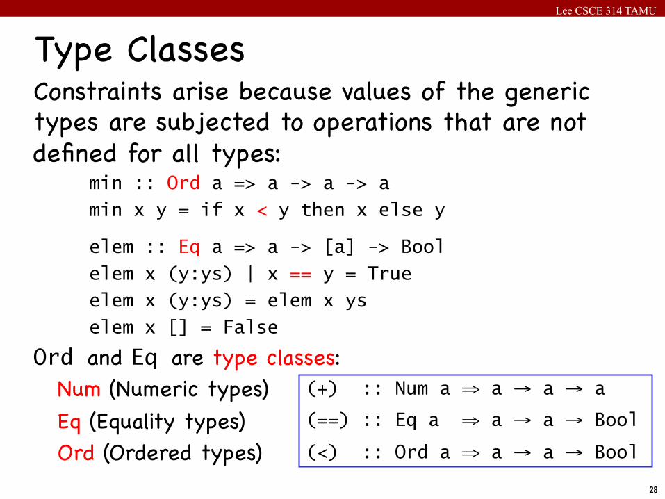
Constraints arise because values of the generic types are subjected to operations that are not defined for all types: min :: Ord a => a -> a -> a

min x y = if x < y then x else y

elem :: Eq a => a -> [a] -> Bool

elem x (y:ys) | x == y = True

elem x (y:ys) = elem x ys

elem x [] = False

Ord and Eq are type classes:Num (Numeric types)Eq (Equality types)Ord (Ordered types)

Type Classes

(+) :: Num a ⇒ a → a → a (==) :: Eq a ⇒ a → a → Bool (<) :: Ord a ⇒ a → a → Bool

Lee CSCE 314 TAMU

29

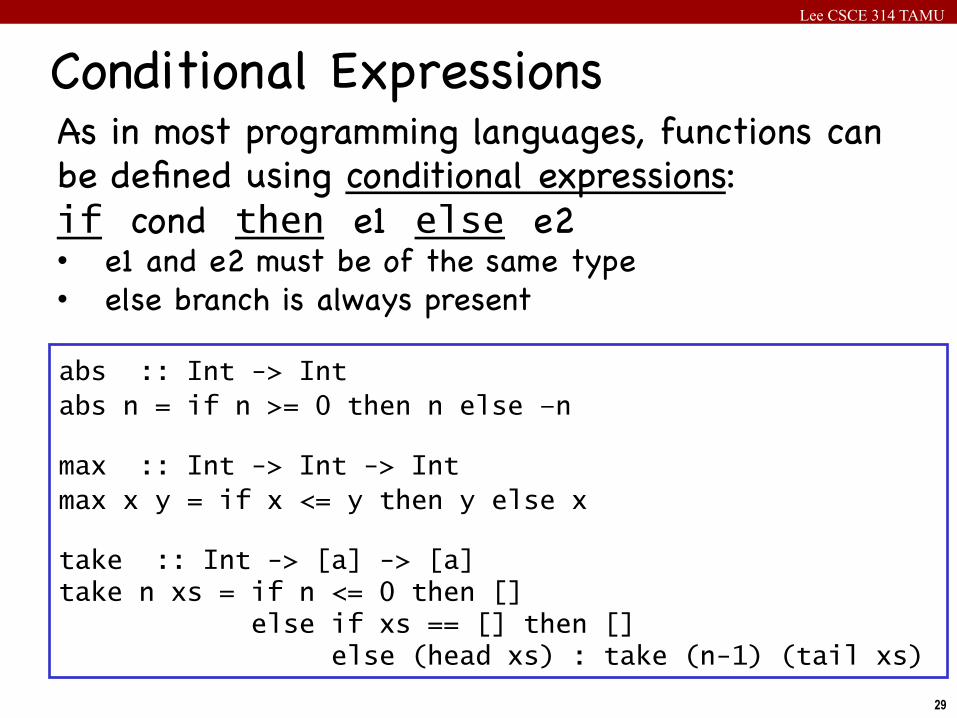
Conditional ExpressionsAs in most programming languages, functions can be defined using conditional expressions:if cond then e1 else e2•  e1 and e2 must be of the same type•  else branch is always present

abs :: Int -> Int abs n = if n >= 0 then n else –n

max :: Int -> Int -> Int max x y = if x <= y then y else x

take :: Int -> [a] -> [a] take n xs = if n <= 0 then [] else if xs == [] then [] else (head xs) : take (n-1) (tail xs)

Lee CSCE 314 TAMU

30

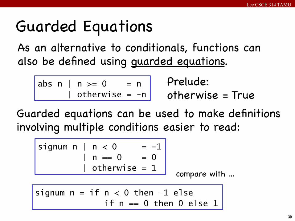
Guarded EquationsAs an alternative to conditionals, functions can also be defined using guarded equations.

abs n | n >= 0 = n | otherwise = -n

Prelude:otherwise = True

Guarded equations can be used to make definitions involving multiple conditions easier to read:

signum n | n < 0 = -1 | n == 0 = 0 | otherwise = 1

signum n = if n < 0 then -1 else if n == 0 then 0 else 1

compare with …

Lee CSCE 314 TAMU

31

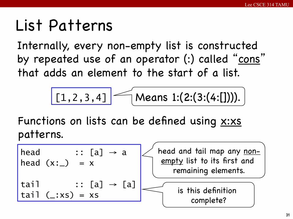
List PatternsInternally, every non-empty list is constructed by repeated use of an operator (:) called “cons” that adds an element to the start of a list.

[1,2,3,4] Means 1:(2:(3:(4:[]))).

Functions on lists can be defined using x:xs patterns.head :: [a] → a head (x:_) = x tail :: [a] → [a] tail (_:xs) = xs

head and tail map any non-empty list to its first and

remaining elements.

is this definition complete?

Lee CSCE 314 TAMU

32

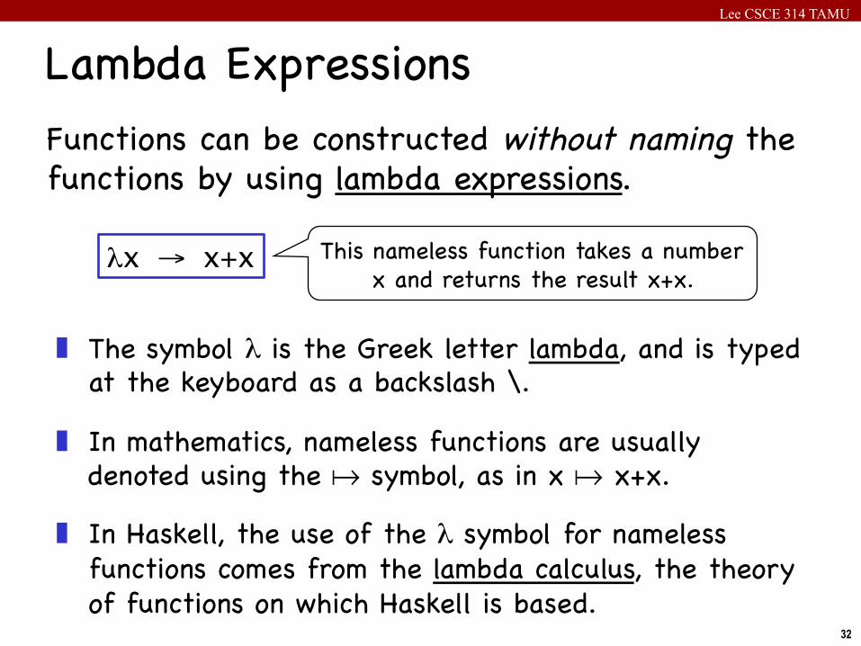
Lambda ExpressionsFunctions can be constructed without naming the functions by using lambda expressions.

λx → x+x This nameless function takes a number x and returns the result x+x.

❚  The symbol λ is the Greek letter lambda, and is typed at the keyboard as a backslash \.

❚  In mathematics, nameless functions are usually denoted using the ! symbol, as in x ! x+x.

❚  In Haskell, the use of the λ symbol for nameless functions comes from the lambda calculus, the theory of functions on which Haskell is based.

Lee CSCE 314 TAMU

33

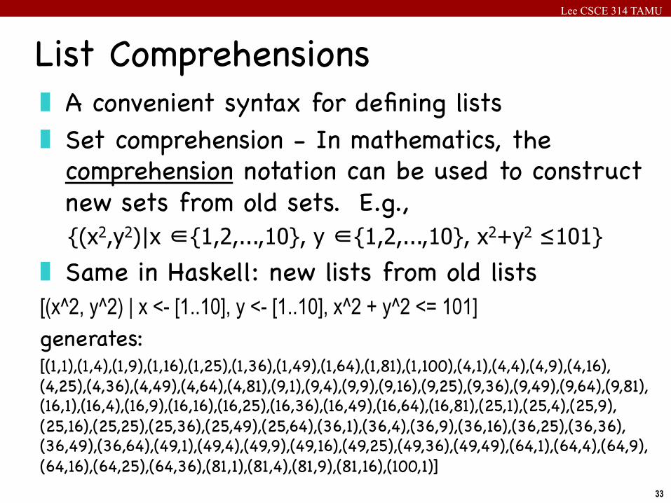
❚  A convenient syntax for defining lists❚  Set comprehension - In mathematics, the

comprehension notation can be used to construct new sets from old sets. E.g.,

{(x2,y2)|x ∈{1,2,...,10}, y ∈{1,2,...,10}, x2+y2 ≤101}❚  Same in Haskell: new lists from old lists[(x^2, y^2) | x <- [1..10], y <- [1..10], x^2 + y^2 <= 101] generates:[(1,1),(1,4),(1,9),(1,16),(1,25),(1,36),(1,49),(1,64),(1,81),(1,100),(4,1),(4,4),(4,9),(4,16),(4,25),(4,36),(4,49),(4,64),(4,81),(9,1),(9,4),(9,9),(9,16),(9,25),(9,36),(9,49),(9,64),(9,81),(16,1),(16,4),(16,9),(16,16),(16,25),(16,36),(16,49),(16,64),(16,81),(25,1),(25,4),(25,9),(25,16),(25,25),(25,36),(25,49),(25,64),(36,1),(36,4),(36,9),(36,16),(36,25),(36,36),(36,49),(36,64),(49,1),(49,4),(49,9),(49,16),(49,25),(49,36),(49,49),(64,1),(64,4),(64,9),(64,16),(64,25),(64,36),(81,1),(81,4),(81,9),(81,16),(100,1)]

List Comprehensions

Lee CSCE 314 TAMU

34

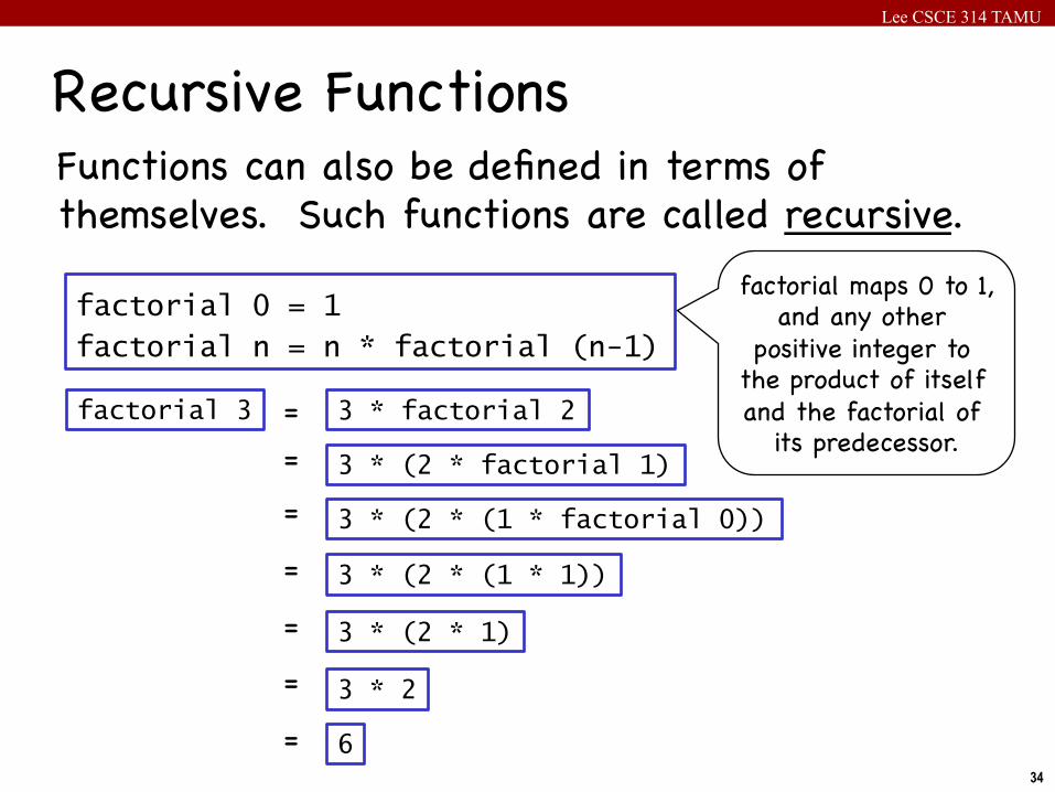
Recursive FunctionsFunctions can also be defined in terms of themselves. Such functions are called recursive.

factorial 0 = 1 factorial n = n * factorial (n-1)

factorial maps 0 to 1, and any other

positive integer to the product of itself and the factorial of

its predecessor.factorial 3 3 * factorial 2

= 3 * (2 * factorial 1)

=

3 * (2 * (1 * factorial 0)) =

3 * (2 * (1 * 1)) =

3 * (2 * 1) =

= 6

3 * 2 =

Lee CSCE 314 TAMU

35

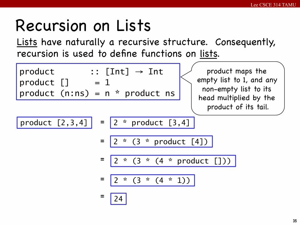
Recursion on ListsLists have naturally a recursive structure. Consequently, recursion is used to define functions on lists.

product :: [Int] → Int product [] = 1 product (n:ns) = n * product ns

product maps the empty list to 1, and any non-empty list to its

head multiplied by the product of its tail.

product [2,3,4] 2 * product [3,4] =

2 * (3 * product [4]) =

2 * (3 * (4 * product [])) =

2 * (3 * (4 * 1)) =

24 =

Lee CSCE 314 TAMU

36

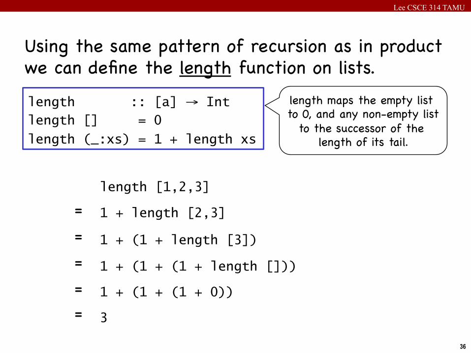
Using the same pattern of recursion as in product we can define the length function on lists.

length :: [a] → Int length [] = 0

length (_:xs) = 1 + length xs

length maps the empty list to 0, and any non-empty list

to the successor of the length of its tail.

length [1,2,3]

1 + length [2,3] =

1 + (1 + length [3]) =

1 + (1 + (1 + length [])) =

1 + (1 + (1 + 0)) =

3 =

Lee CSCE 314 TAMU

37

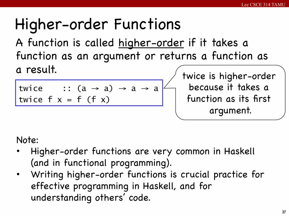
Higher-order FunctionsA function is called higher-order if it takes a function as an argument or returns a function as a result.twice :: (a → a) → a → a twice f x = f (f x)

twice is higher-order because it takes a function as its first

argument.

Note:•  Higher-order functions are very common in Haskell

(and in functional programming).•  Writing higher-order functions is crucial practice for

effective programming in Haskell, and for understanding others’ code.

Lee CSCE 314 TAMU

38

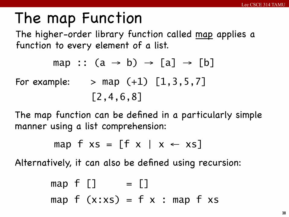
The map FunctionThe higher-order library function called map applies a function to every element of a list.

map :: (a → b) → [a] → [b]

For example: > map (+1) [1,3,5,7]

[2,4,6,8]

The map function can be defined in a particularly simple manner using a list comprehension:

map f xs = [f x | x ← xs]

map f [] = []

map f (x:xs) = f x : map f xs

Alternatively, it can also be defined using recursion:

Lee CSCE 314 TAMU

39

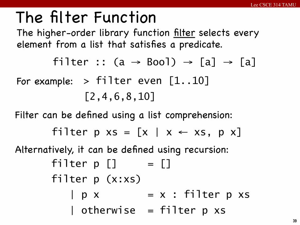
The filter FunctionThe higher-order library function filter selects every element from a list that satisfies a predicate.

filter :: (a → Bool) → [a] → [a]

For example: > filter even [1..10]

[2,4,6,8,10]

Alternatively, it can be defined using recursion:

Filter can be defined using a list comprehension:filter p xs = [x | x ← xs, p x]

filter p [] = []

filter p (x:xs)

| p x = x : filter p xs

| otherwise = filter p xs

Lee CSCE 314 TAMU

40

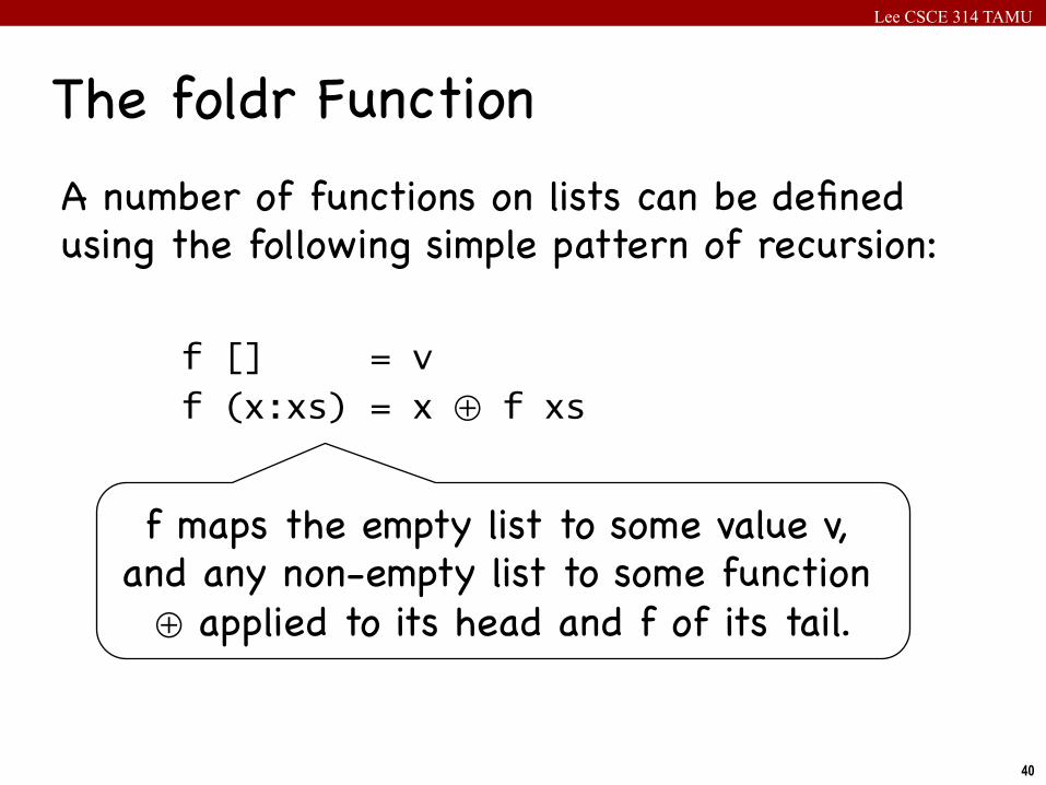
The foldr FunctionA number of functions on lists can be defined using the following simple pattern of recursion:

f [] = v

f (x:xs) = x ⊕ f xs

f maps the empty list to some value v, and any non-empty list to some function ⊕ applied to its head and f of its tail.

Lee CSCE 314 TAMU

41

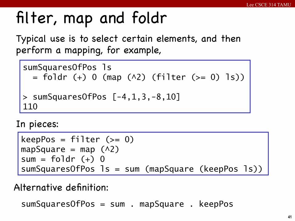
filter, map and foldrTypical use is to select certain elements, and then perform a mapping, for example,sumSquaresOfPos ls = foldr (+) 0 (map (^2) (filter (>= 0) ls)) > sumSquaresOfPos [-4,1,3,-8,10] 110

In pieces:keepPos = filter (>= 0) mapSquare = map (^2) sum = foldr (+) 0 sumSquaresOfPos ls = sum (mapSquare (keepPos ls))

sumSquaresOfPos = sum . mapSquare . keepPos

Alternative definition:

Lee CSCE 314 TAMU

42

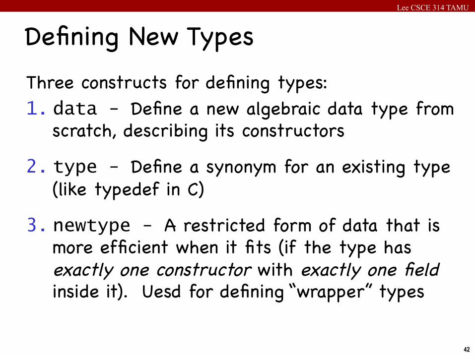
Three constructs for defining types:1. data - Define a new algebraic data type from

scratch, describing its constructors

2. type - Define a synonym for an existing type (like typedef in C)

3. newtype - A restricted form of data that is more efficient when it fits (if the type has exactly one constructor with exactly one field inside it). Uesd for defining “wrapper” types

Defining New Types

Lee CSCE 314 TAMU

43

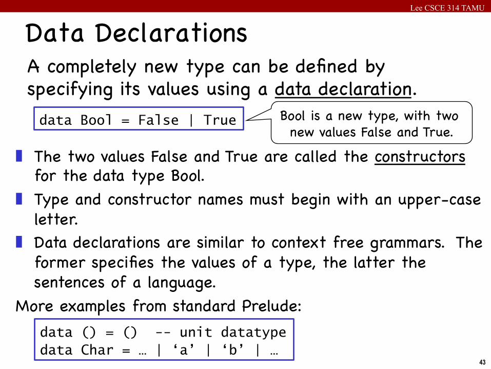
Data DeclarationsA completely new type can be defined by specifying its values using a data declaration.data Bool = False | True Bool is a new type, with two

new values False and True.

❚  The two values False and True are called the constructors for the data type Bool.

❚  Type and constructor names must begin with an upper-case letter.

❚  Data declarations are similar to context free grammars. The former specifies the values of a type, the latter the sentences of a language.

More examples from standard Prelude:data () = () -- unit datatype data Char = … | ‘a’ | ‘b’ | …

Lee CSCE 314 TAMU

44

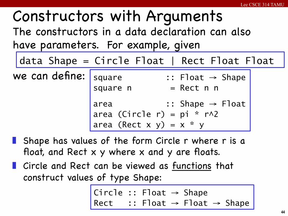
The constructors in a data declaration can also have parameters. For example, givendata Shape = Circle Float | Rect Float Float

square :: Float → Shape square n = Rect n n

area :: Shape → Float area (Circle r) = pi * r^2 area (Rect x y) = x * y

we can define:

Constructors with Arguments

❚  Shape has values of the form Circle r where r is a float, and Rect x y where x and y are floats.

❚  Circle and Rect can be viewed as functions that construct values of type Shape:

Circle :: Float → Shape Rect :: Float → Float → Shape

Lee CSCE 314 TAMU

45

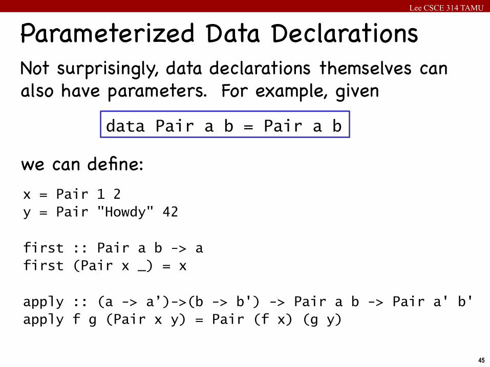
Not surprisingly, data declarations themselves can also have parameters. For example, given

x = Pair 1 2 y = Pair "Howdy" 42 first :: Pair a b -> a first (Pair x _) = x apply :: (a -> a’)->(b -> b') -> Pair a b -> Pair a' b' apply f g (Pair x y) = Pair (f x) (g y)

we can define:

Parameterized Data Declarations

data Pair a b = Pair a b

Lee CSCE 314 TAMU

46

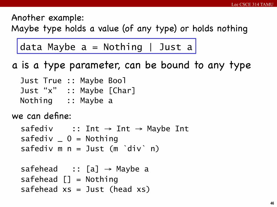
Another example:Maybe type holds a value (of any type) or holds nothing

data Maybe a = Nothing | Just a

safediv :: Int → Int → Maybe Int safediv _ 0 = Nothing safediv m n = Just (m `div` n) safehead :: [a] → Maybe a safehead [] = Nothing safehead xs = Just (head xs)

we can define:

a is a type parameter, can be bound to any typeJust True :: Maybe Bool Just “x” :: Maybe [Char] Nothing :: Maybe a

Lee CSCE 314 TAMU

47

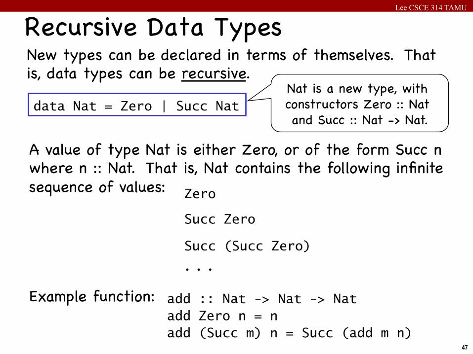
Recursive Data TypesNew types can be declared in terms of themselves. That is, data types can be recursive.

data Nat = Zero | Succ Nat Nat is a new type, with constructors Zero :: Nat and Succ :: Nat -> Nat.

A value of type Nat is either Zero, or of the form Succ n where n :: Nat. That is, Nat contains the following infinite sequence of values:Example function:

Zero

Succ Zero

Succ (Succ Zero)

. . .

add :: Nat -> Nat -> Nat add Zero n = n add (Succ m) n = Succ (add m n)

Lee CSCE 314 TAMU

48

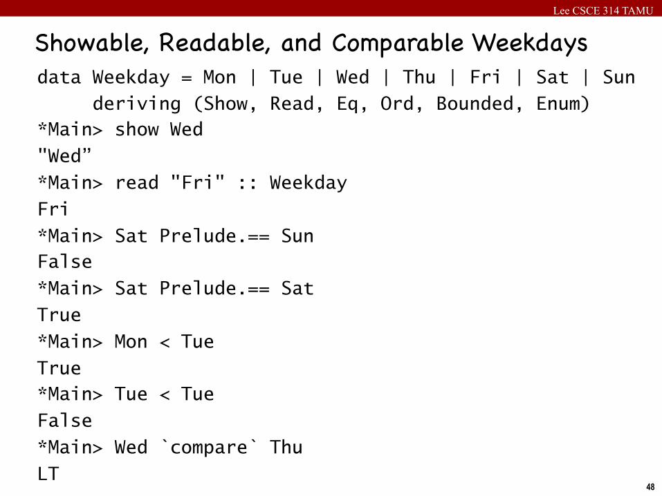
data Weekday = Mon | Tue | Wed | Thu | Fri | Sat | Sun

deriving (Show, Read, Eq, Ord, Bounded, Enum) *Main> show Wed

"Wed”

*Main> read "Fri" :: Weekday

Fri

*Main> Sat Prelude.== Sun False

*Main> Sat Prelude.== Sat

True

*Main> Mon < Tue

True *Main> Tue < Tue

False

*Main> Wed `compare` Thu

LT

Showable, Readable, and Comparable Weekdays

Lee CSCE 314 TAMU

49

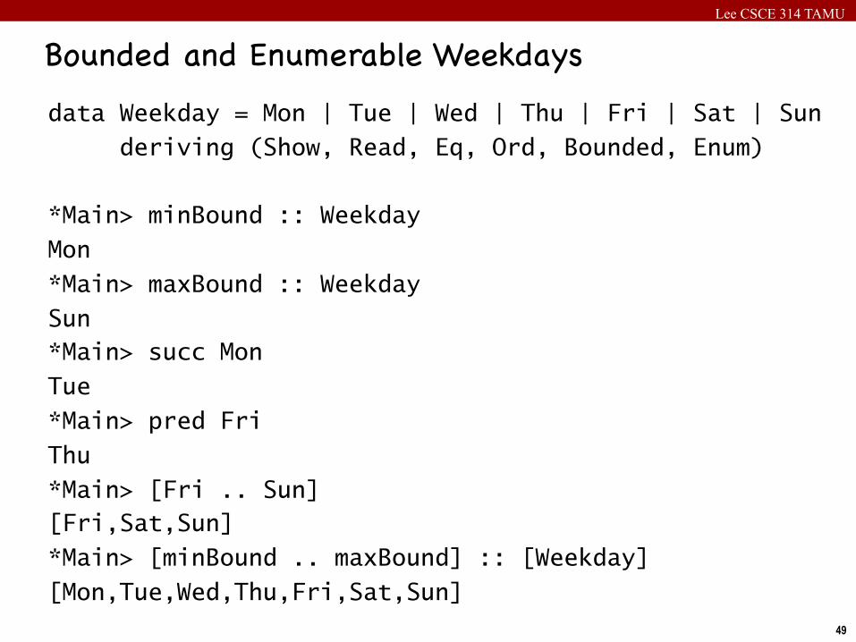
data Weekday = Mon | Tue | Wed | Thu | Fri | Sat | Sun

deriving (Show, Read, Eq, Ord, Bounded, Enum)

*Main> minBound :: Weekday

Mon

*Main> maxBound :: Weekday

Sun *Main> succ Mon

Tue

*Main> pred Fri

Thu

*Main> [Fri .. Sun] [Fri,Sat,Sun]

*Main> [minBound .. maxBound] :: [Weekday]

[Mon,Tue,Wed,Thu,Fri,Sat,Sun]

Bounded and Enumerable Weekdays

Lee CSCE 314 TAMU

50

•  A Haskell program consists of a collection of modules. The purposes of using a module are:1.  To control namespaces.2.  To create abstract data types.

•  A module contains various declarations: First, import declarations, and then, data and type declarations, class and instance declarations, type signatures, function definitions, and so on (in any order)

•  Module names must begin with an uppercase letter

•  One module per file

Modules

Lee CSCE 314 TAMU

51

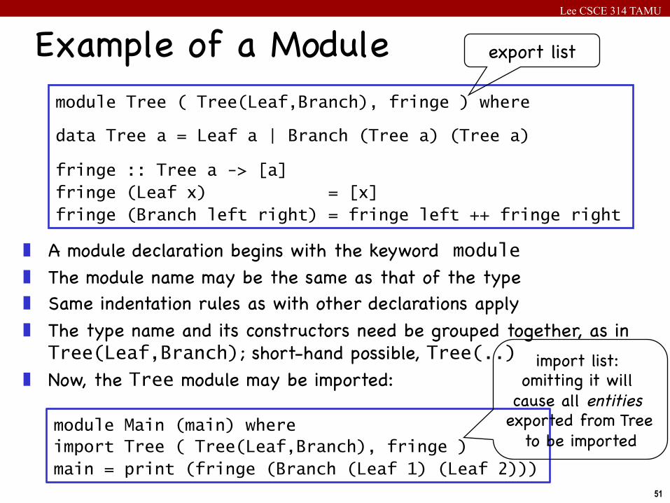
Example of a Modulemodule Tree ( Tree(Leaf,Branch), fringe ) where

data Tree a = Leaf a | Branch (Tree a) (Tree a) 

fringe :: Tree a -> [a] fringe (Leaf x)            = [x] fringe (Branch left right) = fringe left ++ fringe right

❚  A module declaration begins with the keyword module ❚  The module name may be the same as that of the type❚  Same indentation rules as with other declarations apply❚  The type name and its constructors need be grouped together, as in

Tree(Leaf,Branch); short-hand possible, Tree(..) ❚  Now, the Tree module may be imported:

module Main (main) where import Tree ( Tree(Leaf,Branch), fringe ) main = print (fringe (Branch (Leaf 1) (Leaf 2)))

export list

import list: omitting it will

cause all entities exported from Tree

to be imported

Lee CSCE 314 TAMU

52

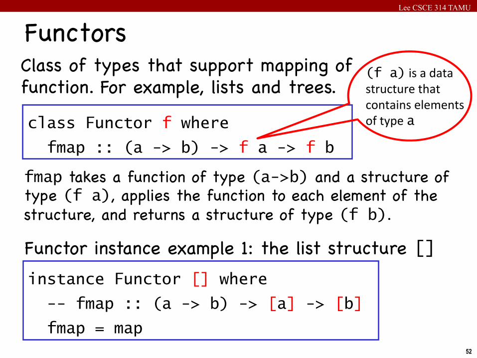
Class of types that support mapping of function. For example, lists and trees.

Functors

class Functor f where

fmap :: (a -> b) -> f a -> f b

fmap takes a function of type (a->b) and a structure of type (f a), applies the function to each element of the structure, and returns a structure of type (f b).

Functor instance example 1: the list structure [] instance Functor [] where

-- fmap :: (a -> b) -> [a] -> [b]

fmap = map

(f a)isadatastructurethatcontainselementsoftypea

Lee CSCE 314 TAMU

53

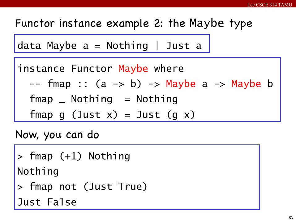
Functor instance example 2: the Maybe type

Now, you can do

> fmap (+1) Nothing

Nothing

> fmap not (Just True)

Just False

data Maybe a = Nothing | Just a

instance Functor Maybe where

-- fmap :: (a -> b) -> Maybe a -> Maybe b

fmap _ Nothing = Nothing

fmap g (Just x) = Just (g x)

Lee CSCE 314 TAMU

54

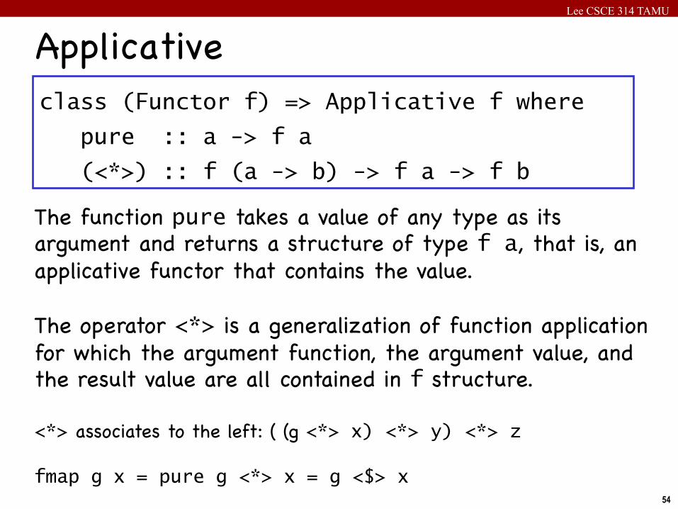
Applicative

The function pure takes a value of any type as its argument and returns a structure of type f a, that is, an applicative functor that contains the value.The operator <*> is a generalization of function application for which the argument function, the argument value, and the result value are all contained in f structure.<*> associates to the left: ( (g <*> x) <*> y) <*> z fmap g x = pure g <*> x = g <$> x

class (Functor f) => Applicative f where

pure :: a -> f a

(<*>) :: f (a -> b) -> f a -> f b

Lee CSCE 314 TAMU

55

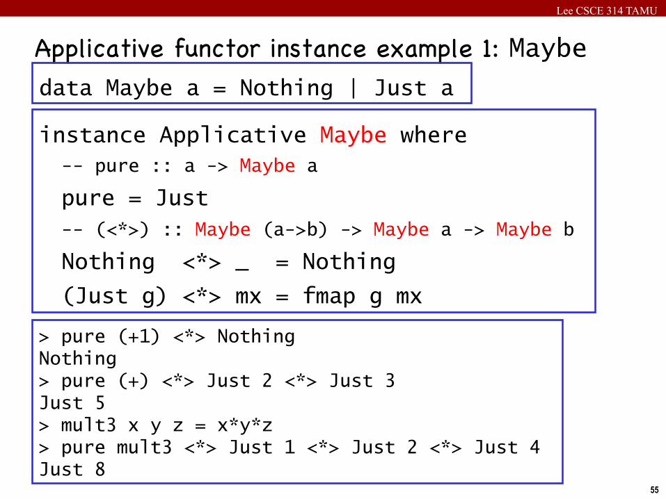
Applicative functor instance example 1: Maybe

> pure (+1) <*> Nothing Nothing > pure (+) <*> Just 2 <*> Just 3 Just 5 > mult3 x y z = x*y*z > pure mult3 <*> Just 1 <*> Just 2 <*> Just 4 Just 8

data Maybe a = Nothing | Just a

instance Applicative Maybe where -- pure :: a -> Maybe a

pure = Just -- (<*>) :: Maybe (a->b) -> Maybe a -> Maybe b

Nothing <*> _ = Nothing

(Just g) <*> mx = fmap g mx

Lee CSCE 314 TAMU

56

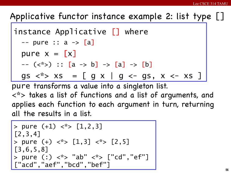
Applicative functor instance example 2: list type []

> pure (+1) <*> [1,2,3] [2,3,4] > pure (+) <*> [1,3] <*> [2,5] [3,6,5,8] > pure (:) <*> "ab" <*> ["cd","ef"] ["acd","aef","bcd","bef"]

instance Applicative [] where -- pure :: a -> [a]

pure x = [x] -- (<*>) :: [a -> b] -> [a] -> [b]

gs <*> xs = [ g x | g <- gs, x <- xs ] pure transforms a value into a singleton list.<*> takes a list of functions and a list of arguments, and applies each function to each argument in turn, returning all the results in a list.

Lee CSCE 314 TAMU

57

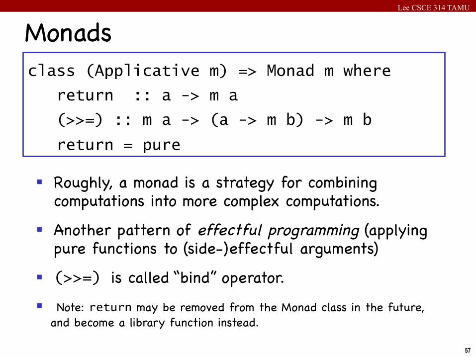
Monads

§  Roughly, a monad is a strategy for combining computations into more complex computations.

§  Another pattern of effectful programming (applying pure functions to (side-)effectful arguments)

§  (>>=) is called “bind” operator.

§  Note: return may be removed from the Monad class in the future, and become a library function instead.

class (Applicative m) => Monad m where

return :: a -> m a

(>>=) :: m a -> (a -> m b) -> m b

return = pure

Lee CSCE 314 TAMU

58

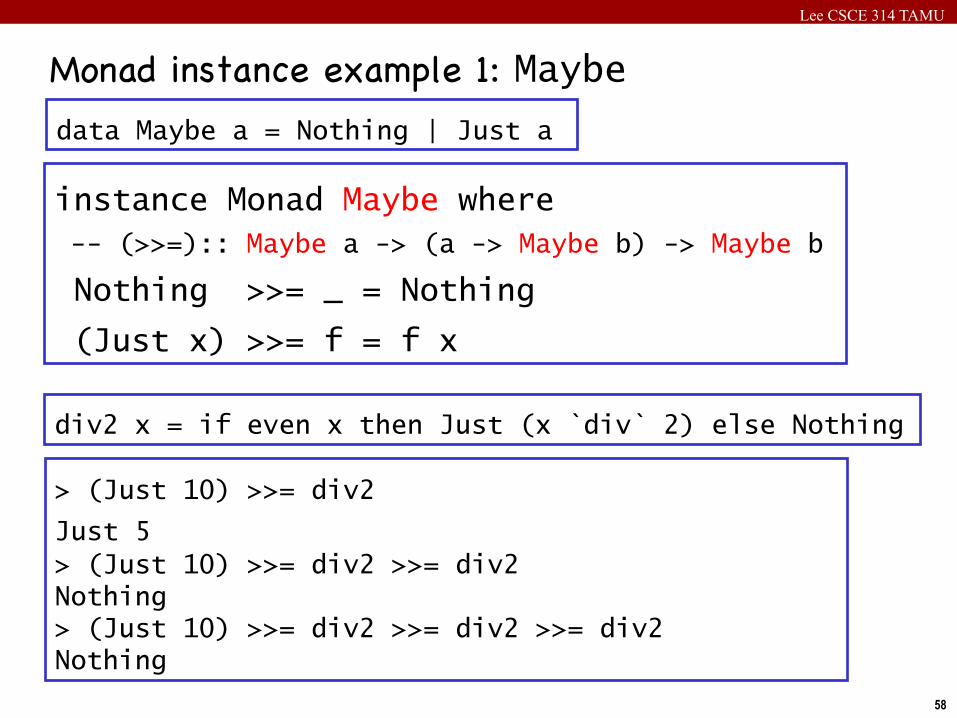
Monad instance example 1: Maybedata Maybe a = Nothing | Just a

instance Monad Maybe where -- (>>=):: Maybe a -> (a -> Maybe b) -> Maybe b

Nothing >>= _ = Nothing

(Just x) >>= f = f x

> (Just 10) >>= div2

Just 5 > (Just 10) >>= div2 >>= div2 Nothing > (Just 10) >>= div2 >>= div2 >>= div2 Nothing

div2 x = if even x then Just (x `div` 2) else Nothing

Lee CSCE 314 TAMU

59

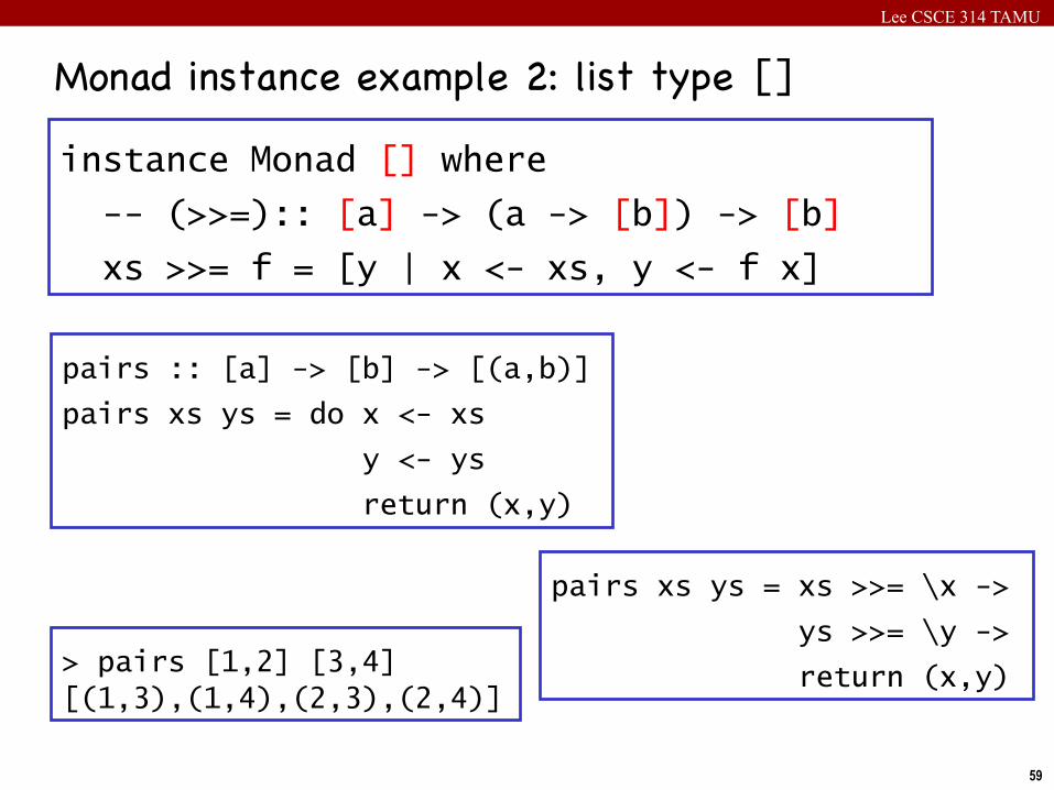
Monad instance example 2: list type []

instance Monad [] where

-- (>>=):: [a] -> (a -> [b]) -> [b]

xs >>= f = [y | x <- xs, y <- f x]

> pairs [1,2] [3,4] [(1,3),(1,4),(2,3),(2,4)]

pairs :: [a] -> [b] -> [(a,b)]

pairs xs ys = do x <- xs

y <- ys

return (x,y)

pairs xs ys = xs >>= \x ->

ys >>= \y ->

return (x,y)

Lee CSCE 314 TAMU

60

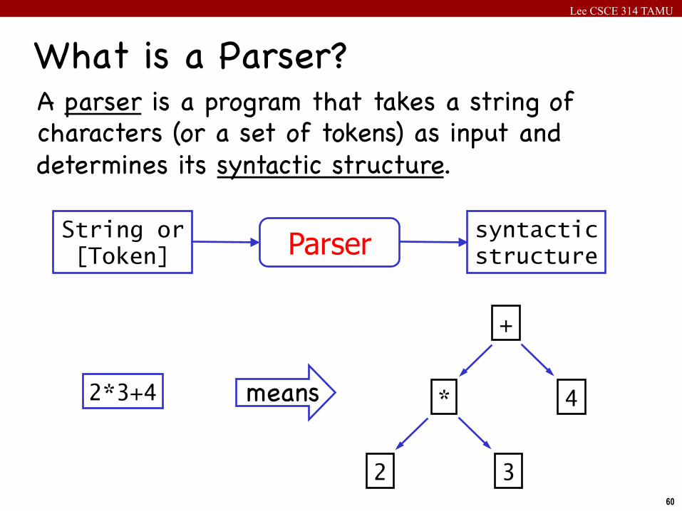
What is a Parser?A parser is a program that takes a string of characters (or a set of tokens) as input and determines its syntactic structure.

2*3+4 means 4

+

*

3 2

String or [Token] Parser syntactic

structure

Lee CSCE 314 TAMU

61

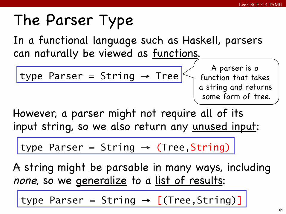
The Parser TypeIn a functional language such as Haskell, parsers can naturally be viewed as functions.

type Parser = String → Tree A parser is a

function that takes a string and returns some form of tree.

However, a parser might not require all of its input string, so we also return any unused input:

type Parser = String → (Tree,String)

A string might be parsable in many ways, including none, so we generalize to a list of results:

type Parser = String → [(Tree,String)]

Lee CSCE 314 TAMU

62

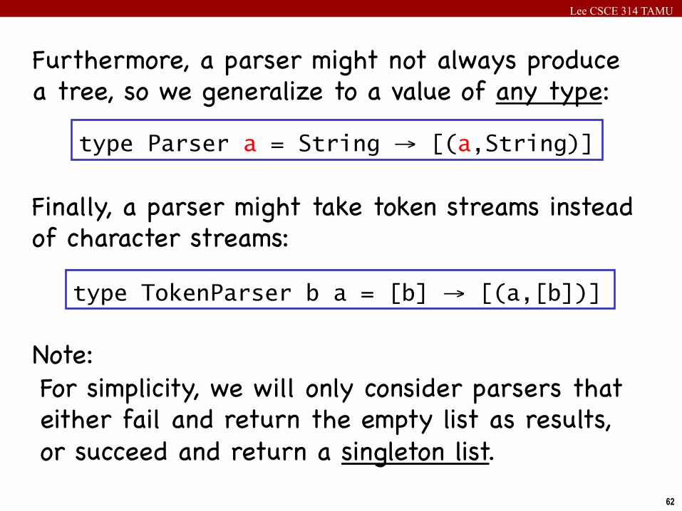
Furthermore, a parser might not always produce a tree, so we generalize to a value of any type:

type Parser a = String → [(a,String)]

Note:For simplicity, we will only consider parsers that either fail and return the empty list as results, or succeed and return a singleton list.

Finally, a parser might take token streams instead of character streams:

type TokenParser b a = [b] → [(a,[b])]

Lee CSCE 314 TAMU

63

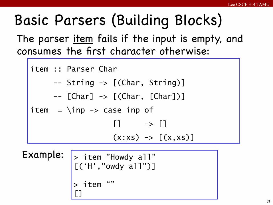
Basic Parsers (Building Blocks)The parser item fails if the input is empty, and consumes the first character otherwise:

item :: Parser Char

-- String -> [(Char, String)]

-- [Char] -> [(Char, [Char])]

item = \inp -> case inp of

[] -> []

(x:xs) -> [(x,xs)]

> item ”Howdy all" [(‘H',”owdy all")] > item “” []

Example:

Lee CSCE 314 TAMU

64

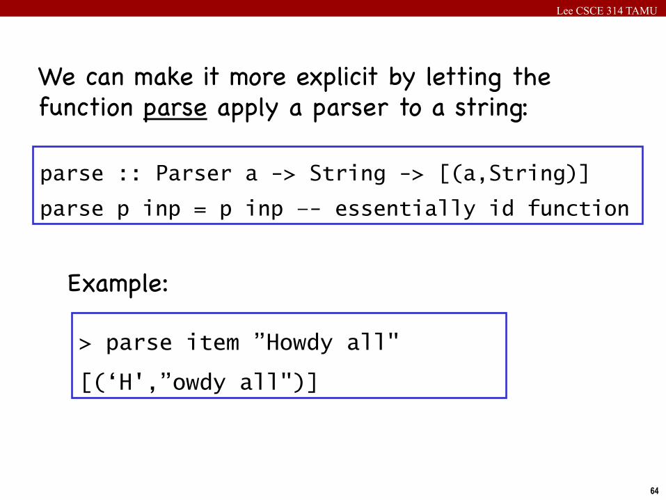
We can make it more explicit by letting the function parse apply a parser to a string:

parse :: Parser a -> String -> [(a,String)]

parse p inp = p inp –- essentially id function

> parse item ”Howdy all"

[(‘H',”owdy all")]

Example:

Lee CSCE 314 TAMU

65

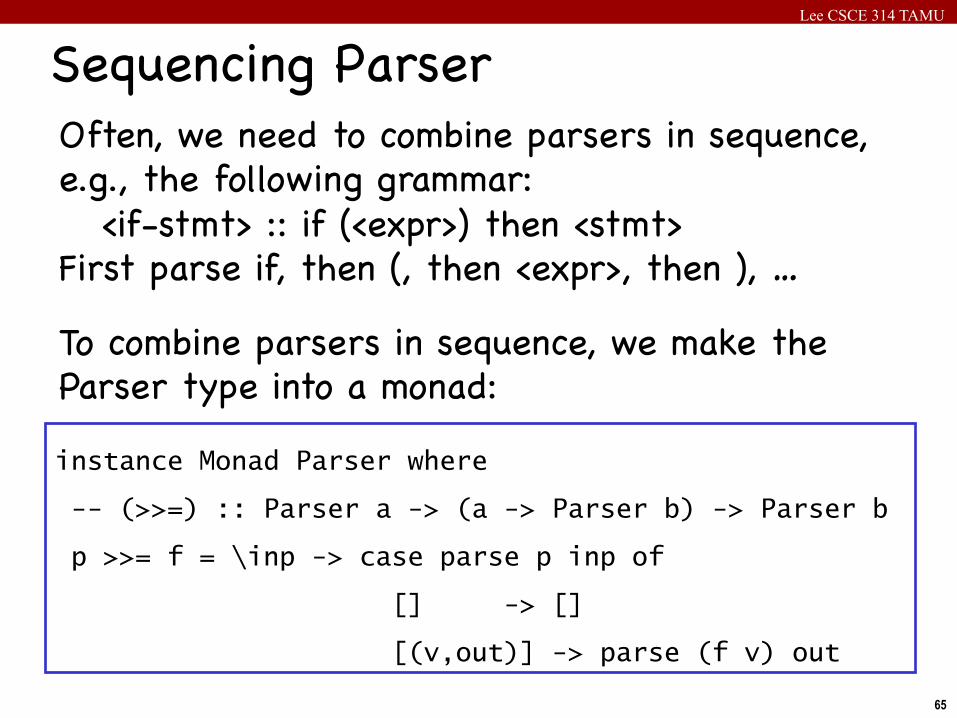
Sequencing ParserOften, we need to combine parsers in sequence, e.g., the following grammar: <if-stmt> :: if (<expr>) then <stmt>First parse if, then (, then <expr>, then ), …

To combine parsers in sequence, we make the Parser type into a monad:instance Monad Parser where

-- (>>=) :: Parser a -> (a -> Parser b) -> Parser b

p >>= f = \inp -> case parse p inp of

[] -> []

[(v,out)] -> parse (f v) out

Lee CSCE 314 TAMU

66

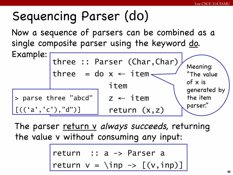
Now a sequence of parsers can be combined as a single composite parser using the keyword do.Example:

Sequencing Parser (do)

three :: Parser (Char,Char)

three = do x ← item

item

z ← item

return (x,z)

Meaning: “The value of x is generated by the item parser.”

> parse three ”abcd"

[((‘a',’c’),”d")]

The parser return v always succeeds, returning the value v without consuming any input:

return :: a -> Parser a

return v = \inp -> [(v,inp)]

Lee CSCE 314 TAMU

67

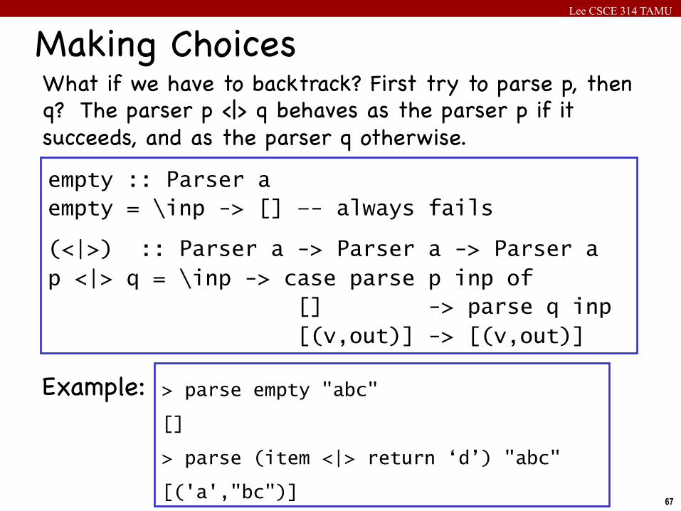
What if we have to backtrack? First try to parse p, then q? The parser p <|> q behaves as the parser p if it succeeds, and as the parser q otherwise.

empty :: Parser a empty = \inp -> [] –- always fails

(<|>) :: Parser a -> Parser a -> Parser a p <|> q = \inp -> case parse p inp of [] -> parse q inp [(v,out)] -> [(v,out)]

Making Choices

> parse empty "abc"

[]

> parse (item <|> return ‘d’) "abc"

[('a',"bc")]

Example:

Lee CSCE 314 TAMU

68

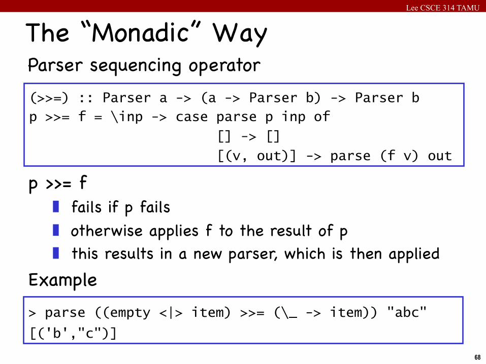
The “Monadic” Way

(>>=) :: Parser a -> (a -> Parser b) -> Parser b p >>= f = \inp -> case parse p inp of

[] -> []

[(v, out)] -> parse (f v) out

Parser sequencing operator

p >>= f❚  fails if p fails❚  otherwise applies f to the result of p❚  this results in a new parser, which is then applied

Example> parse ((empty <|> item) >>= (\_ -> item)) "abc"

[('b',"c")]

Lee CSCE 314 TAMU

69

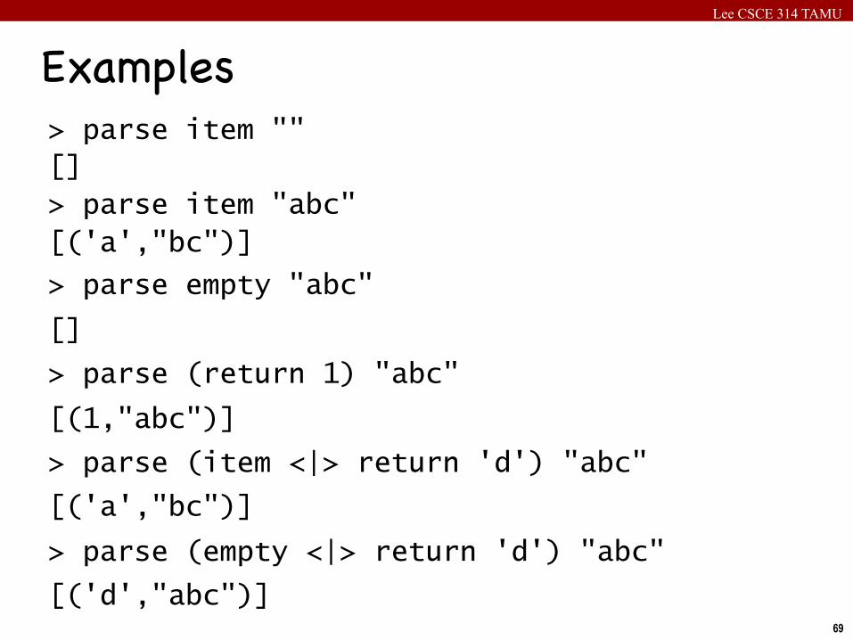
> parse item "" []

> parse item "abc" [('a',"bc")]

> parse empty "abc"

[]

> parse (return 1) "abc"

[(1,"abc")]

> parse (item <|> return 'd') "abc"

[('a',"bc")]

> parse (empty <|> return 'd') "abc"

[('d',"abc")]

Examples

Lee CSCE 314 TAMU

70

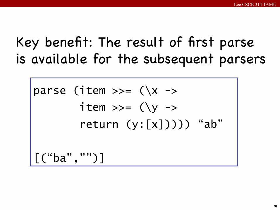
Key benefit: The result of first parse is available for the subsequent parsers

parse (item >>= (\x ->

item >>= (\y ->

return (y:[x])))) “ab”

[(“ba”,””)]