Embed Size (px)
Citation preview
CSCI 252: Neural Networks and
Graphical ModelsFall Term 2016
Prof. Levy
Architecture #2:The Hopfield Network
(Hopfield 1982; notes from Dayhoff 1990)
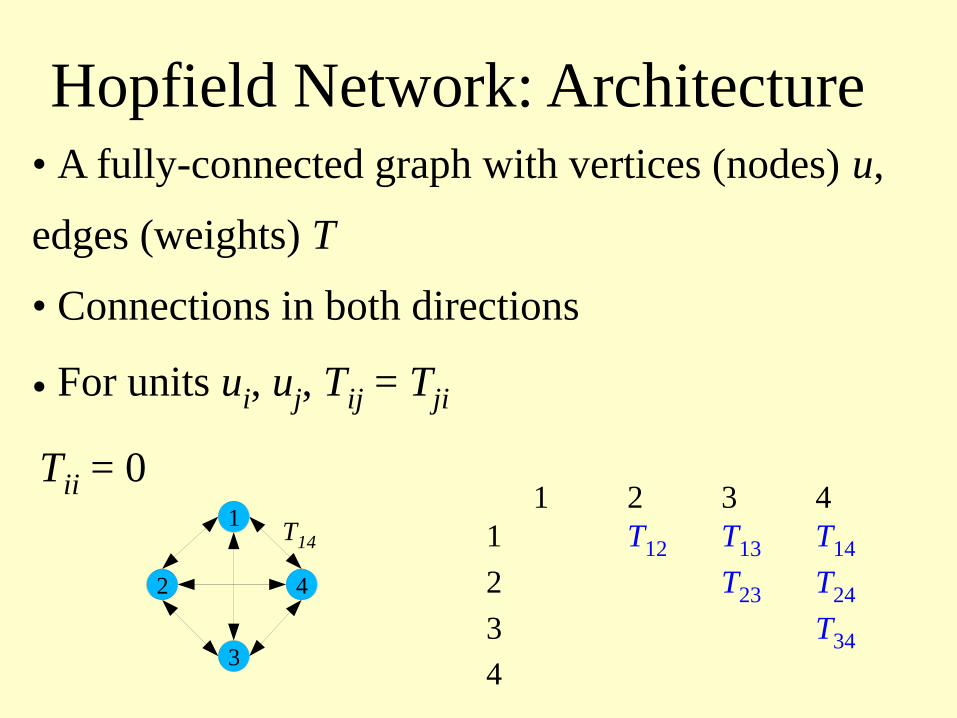
Hopfield Network: Architecture• A fully-connected graph with vertices (nodes) u,
edges (weights) T
• Connections in both directions
• For units ui, uj, Tij = Tji
Tii = 01
3
2 4
T14
1 2 3 41 T12 T13 T14
2 T23 T24
3 T34
4
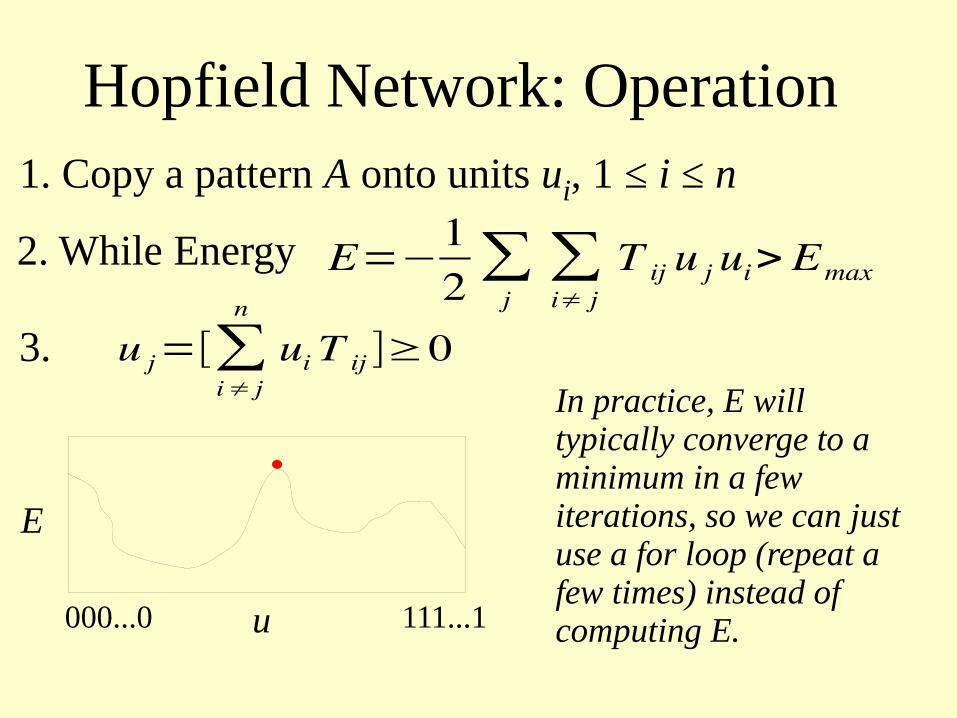
Hopfield Network: Operation
2. While Energy E=−12∑
j∑i≠ j
T ij u j ui> Emax
1. Copy a pattern A onto units ui, 1 ≤ i ≤ n
3. u j=[∑i≠ j
n
ui T ij ]≥0
u
E
000...0 111...1
In practice, E will typically converge to a minimum in a few iterations, so we can just use a for loop (repeat a few times) instead of computing E.
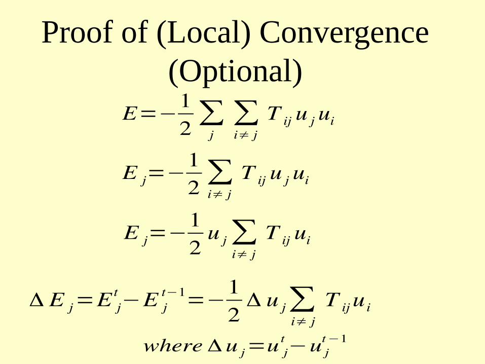
Proof of (Local) Convergence (Optional)
E=−12∑
j∑i≠ j
T ij u j ui
E j=−12∑i≠ j
T ij u j ui
E j=−12
u j∑i≠ j
T ij ui
Δ E j=E jt−E j
t−1=−
12
Δ u j∑i≠ j
T ij u i
where Δu j=u jt−u j
t−1
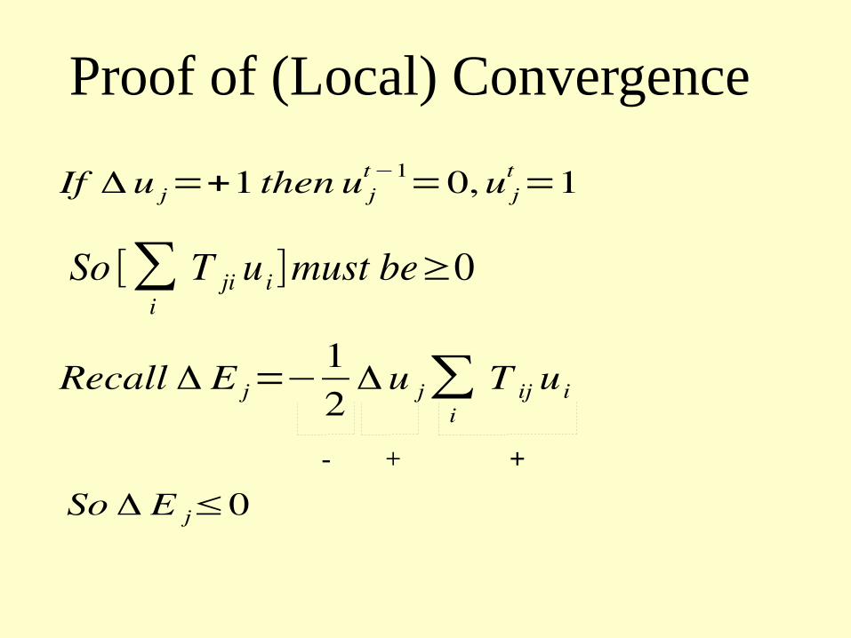
Proof of (Local) Convergence
If Δu j=+1 then u jt−1
=0,u jt=1
So [∑i
T ji u i ]must be≥0
Recall Δ E j=−12
Δu j∑i
T ij u i
- + +
So Δ E j≤0

Proof of (Local) Convergence
If Δu j=−1 then u jt−1
=1, u jt=0
So [∑i
T ji u i ]must be<0
Δ E j=−12
Δu j∑i
T ij ui
- - -
So Δ E j≤0
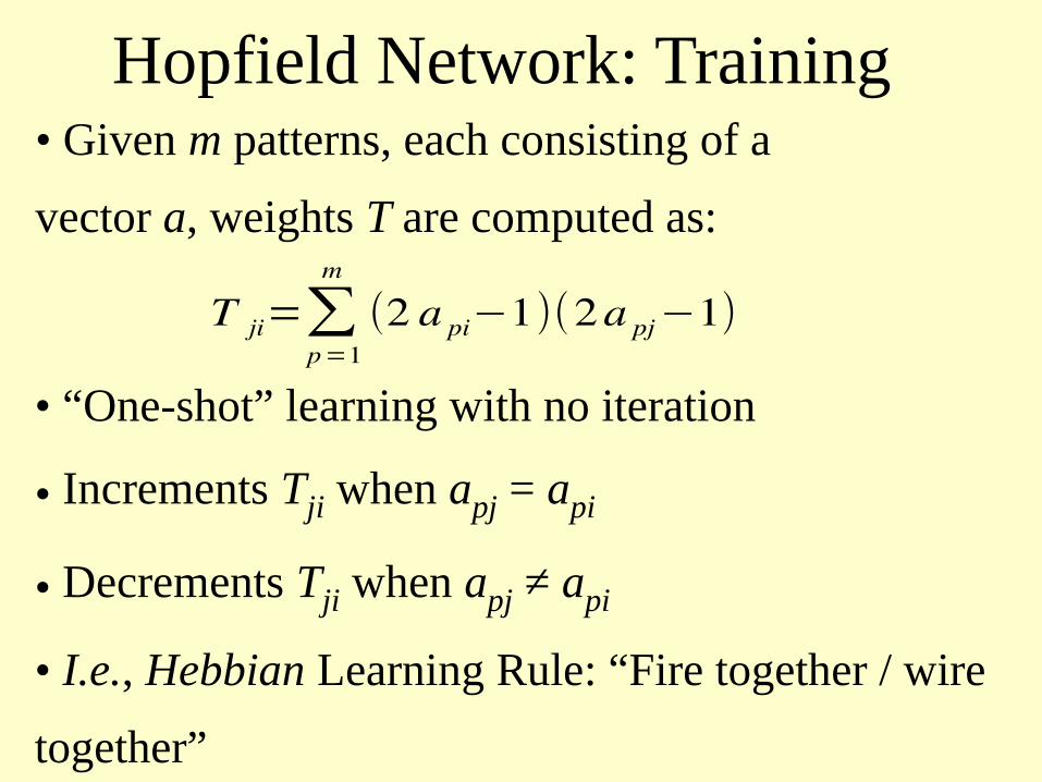
Hopfield Network: Training
T ji=∑p=1
m
(2 a pi−1)(2a pj−1)
• “One-shot” learning with no iteration
• Increments Tji when apj = api
• Decrements Tji when apj ≠ api
• I.e., Hebbian Learning Rule: “Fire together / wire
together”
• Given m patterns, each consisting of a
vector a, weights T are computed as:
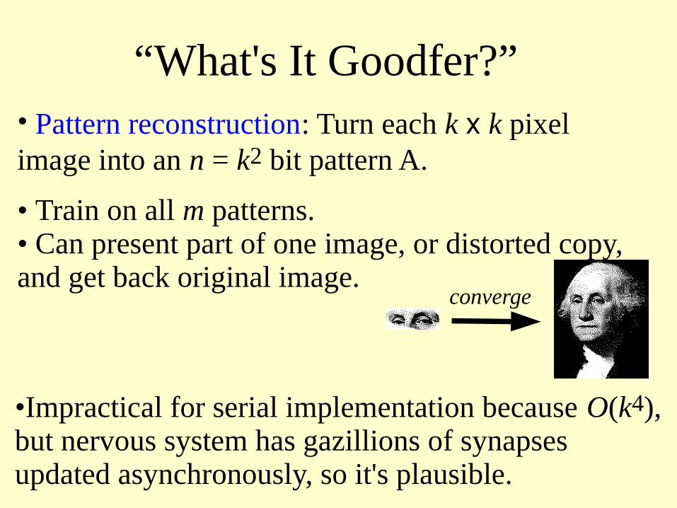
“What's It Goodfer?”• Pattern reconstruction: Turn each k x k pixel image into an n = k2 bit pattern A.
• Train on all m patterns.• Can present part of one image, or distorted copy, and get back original image.
converge
•Impractical for serial implementation because O(k4), but nervous system has gazillions of synapses updated asynchronously, so it's plausible.
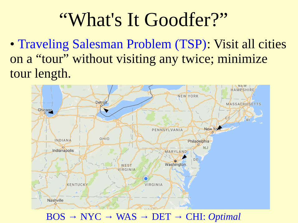
“What's It Goodfer?”• Traveling Salesman Problem (TSP): Visit all cities on a “tour” without visiting any twice; minimize tour length.
BOS → NYC → WAS → DET → CHI: Optimal
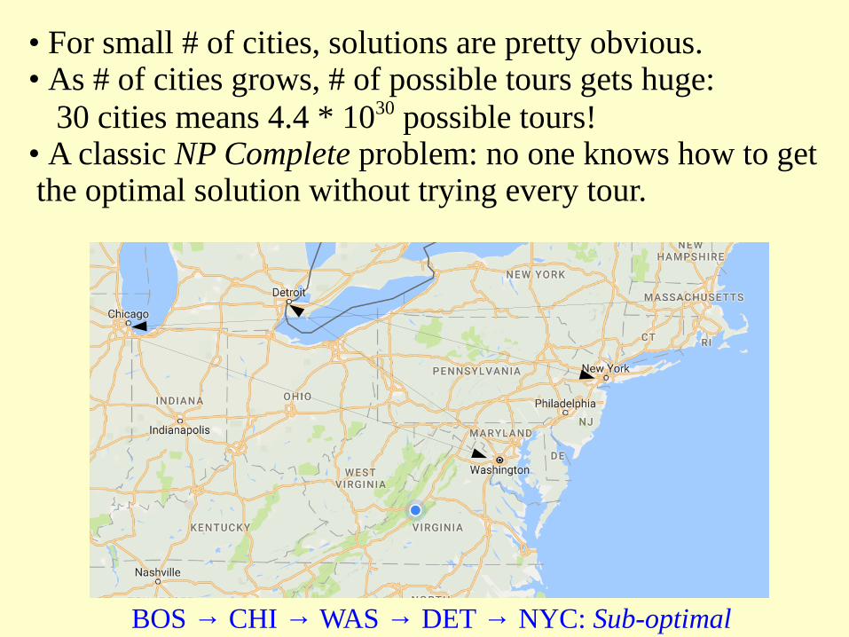
BOS → CHI → WAS → DET → NYC: Sub-optimal
• For small # of cities, solutions are pretty obvious.• As # of cities grows, # of possible tours gets huge: 30 cities means 4.4 * 1030 possible tours!
• A classic NP Complete problem: no one knows how to get the optimal solution without trying every tour.
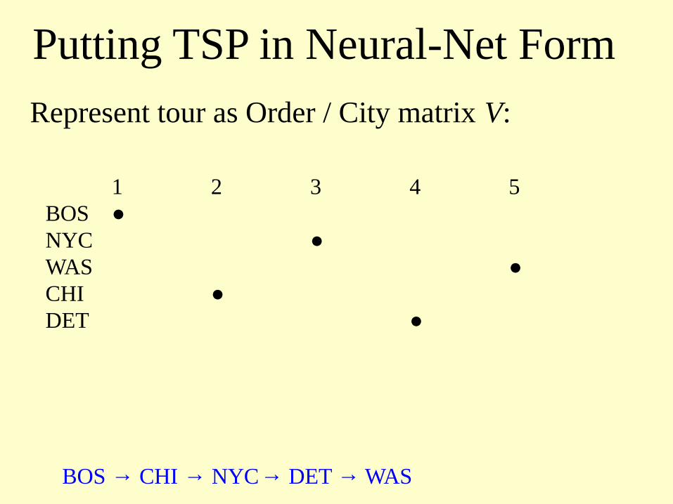
Represent tour as Order / City matrix V:
1 2 3 4 5BOS ●NYC ●WAS ●CHI ●DET ●
BOS → CHI → NYC→ DET → WAS
Putting TSP in Neural-Net Form
• Hopfield & Tank (1985) : Use continuous-time convergence algorithm (w/sigmoid squashing function) to solve TSP.
• For N cities, have N2 units, where each unit represents a city/order combination (5 cities gives 25 units)
• Hence it is possible to represent situations that are logically impossible: e.g., both Boston and New York as #2 in the tour. This is in fact how the network starts at time zero.
• So the trick is to create an energy function that penalizes (assigns high energy to) impossible situations and situations violating the constraints of the TSP (longer total distance than necessary).
• Let’s build this energy function one constraint at a time ….
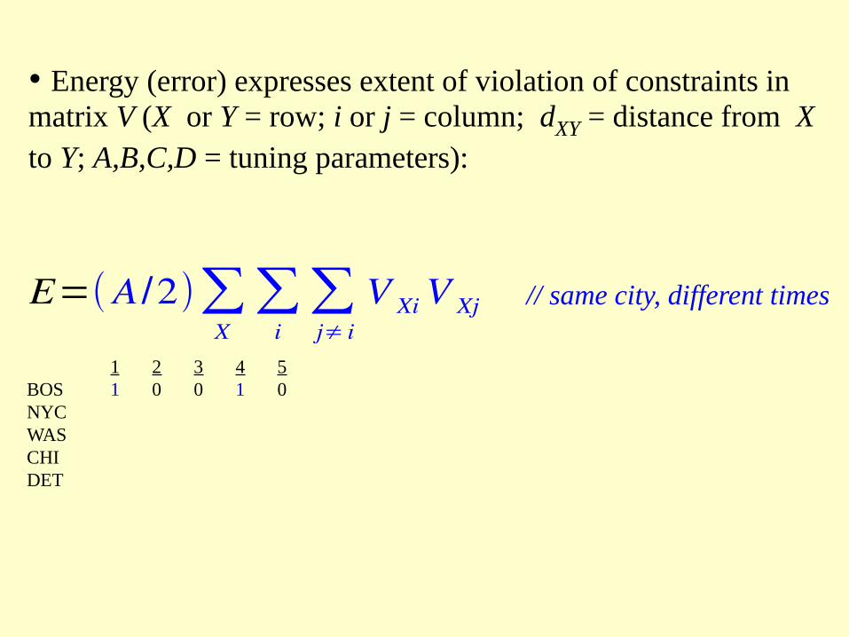
• Energy (error) expresses extent of violation of constraints in matrix V (X or Y = row; i or j = column; dXY = distance from X to Y; A,B,C,D = tuning parameters):
E=( A/2)∑X∑
i∑j≠ i
V Xi V Xj // same city, different times
1 2 3 4 5BOS 1 0 0 1 0NYCWAS CHIDET
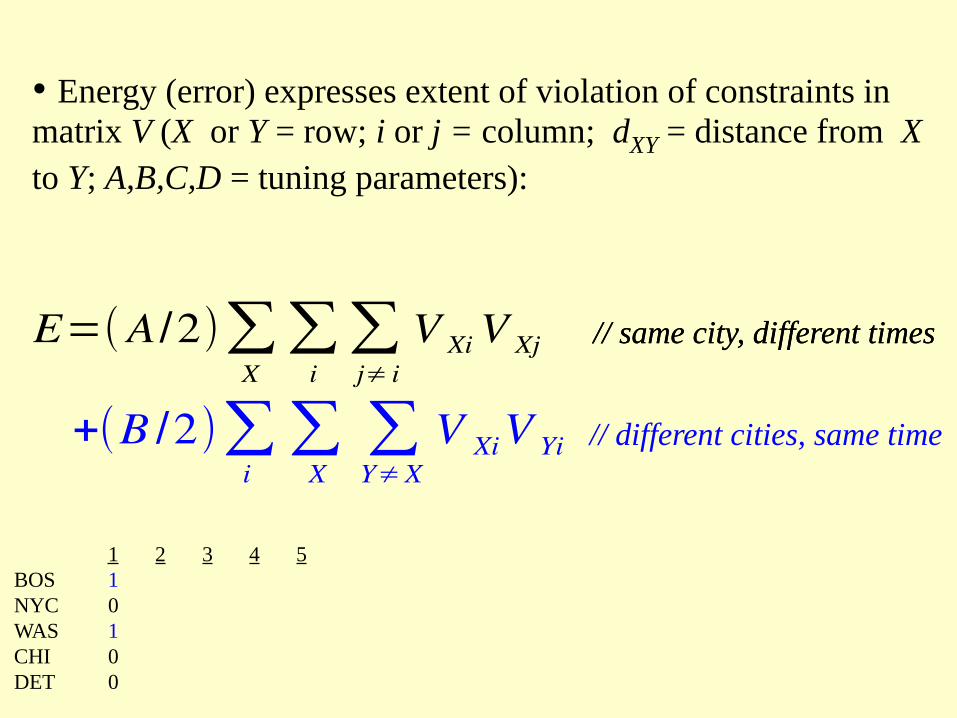
// same city, different times
+(B /2)∑i∑
X∑Y≠X
V XiV Yi // different cities, same time
• Energy (error) expresses extent of violation of constraints in matrix V (X or Y = row; i or j = column; dXY = distance from X to Y; A,B,C,D = tuning parameters):
E=( A/2)∑X∑
i∑j≠ i
V Xi V Xj // same city, different times
1 2 3 4 5BOS 1NYC 0WAS 1 CHI 0DET 0
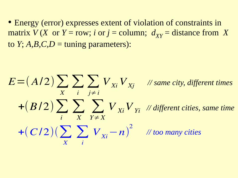
+(B /2)∑i∑
X∑Y≠X
V XiV Yi // different cities, same time
+(C /2)(∑X
∑i
V Xi−n)2
// too many cities
• Energy (error) expresses extent of violation of constraints in matrix V (X or Y = row; i or j = column; dXY = distance from X to Y; A,B,C,D = tuning parameters):
E=( A/2)∑X∑
i∑j≠ i
V Xi V Xj // same city, different times
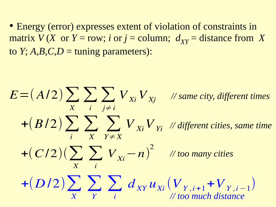
+(B /2)∑i∑
X∑Y≠X
V XiV Yi // different cities, same time
+(C /2)(∑X
∑i
V Xi−n)2
// too many cities
+(D /2)∑X∑
Y∑
id XY uXi (V Y ,i+1+V Y ,i−1)
// too much distance
• Energy (error) expresses extent of violation of constraints in matrix V (X or Y = row; i or j = column; dXY = distance from X to Y; A,B,C,D = tuning parameters):
E=( A/2)∑X∑
i∑j≠ i
V Xi V Xj // same city, different times
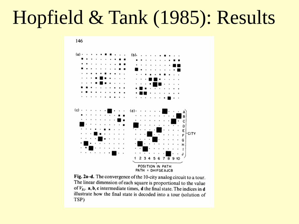
Hopfield & Tank (1985): Results
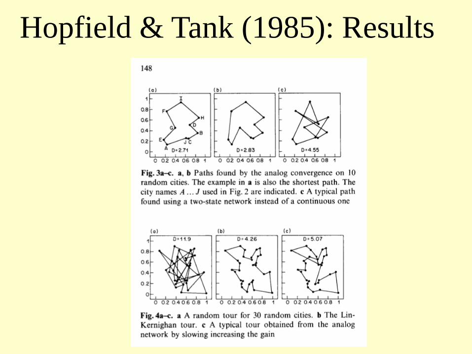
Hopfield & Tank (1985): Results
Boltzmann Learning (Hinton & Sejnowski 1986)
u
E
000...0 111...1
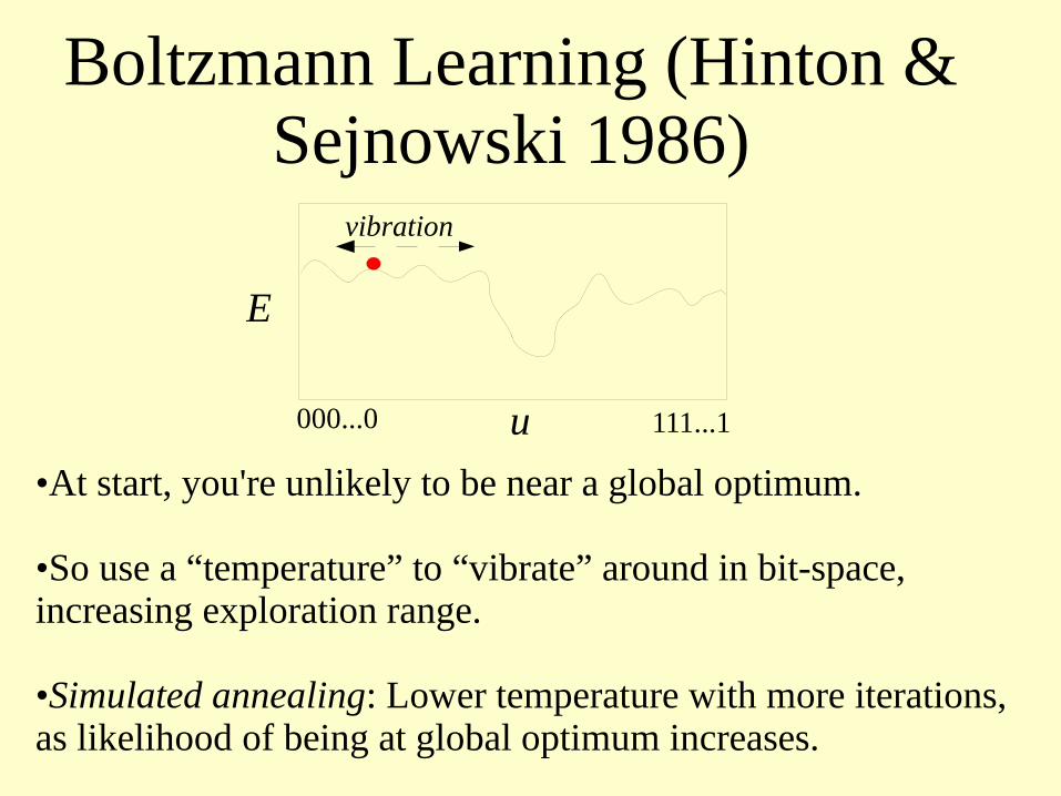
•At start, you're unlikely to be near a global optimum.
•So use a “temperature” to “vibrate” around in bit-space, increasing exploration range.
•Simulated annealing: Lower temperature with more iterations, as likelihood of being at global optimum increases.
vibration